statistical methods for reducing bias in web surveys - statistics and
TRANSCRIPT

STATISTICAL METHODS FOR
REDUCING BIAS IN WEB SURVEYS
by
Myoung Ho Lee
B.Eng., Seoul National University, 1996
a Project submitted in partial fulfillment
of the requirements for the degree of
Master of Science
in the
Department of Statistics and Actuarial Science
Faculty of Science
c© Myoung Ho Lee 2011
Simon Fraser University
Summer 2011
All rights reserved.
However, in accordance with the Copyright Act of Canada, this work may be
reproduced without authorization under the conditions for “Fair Dealing.”
Therefore, limited reproduction of this work for the purposes of private study,
research, criticism, review and news reporting is likely to be in accordance with
the law, particularly if cited appropriately.

APPROVAL
Name: Myoung Ho Lee
Degree: Master of Science
Title of Project: STATISTICAL METHODS FOR REDUCING BIAS IN WEB
SURVEYS
Examining Committee: Dr. Derek Bingham
Chair
Dr. Thomas M. Loughin, Senior Supervisor
Dr. Steven K. Thompson, Supervisor
Dr. Lawrence McCandless, External Examiner,
Professor of Health Science,
Simon Fraser University
Date Approved:
ii

Abstract
Web surveys have become popular recently because of their attractive advantages of data
collection. However, in web surveys, bias may occur mainly due to limited coverage and
self-selection. This paper reviews characteristics and problems of web surveys, and describes
some adjustment weighting methods for reducing the bias. Propensity score adjustment is
used for correcting selection bias due to non-probability sampling, and calibration adjust-
ment is used for correction coverage bias. Those bias reduction methods will be explored
by comparing face-to-face survey (reference survey) results with web survey results for the
Social Survey produced by Statistics Korea. The methods studied include different variable
selection methods for propensity score calculation and different propensity score weighting
methods.
Keywords: Web survey; non-probability; self-selection; under-coverage; propensity score
adjustment; calibration
iii

To my beloved wife and two adorable daughters!
iv

Acknowledgments
I would like to express my deepest gratitude to my supervisor, Dr. Thomas M. Loughin who
made great effort to guide me throughout my studies. This project would not have been
possible without his continuous guidance and support. I would also like to thank Dr. Steven
K. Thompson for teaching me sampling theory and practice. What I learned from his class
became basic knowledge to conduct this project. I appreciate Dr. Lawrence McCandless
for providing valuable suggestions and advice on my project.
Furthermore, I would like to thank all the professors in the Department of Statistics
and Actuarial Science for helping me discover my interest in statistics. Actually, I had little
knowledge of statistics before coming at Simon Fraser University. All I have learned here
will give me a good opportunity for my future career.
I am also thankful to the department staff and fellow graduate students who have sup-
ported me throughout my graduate program. In particular, I am so grateful to Jean Shin
for helping me to complete my project. In addition, I would like to thank staff of Statistics
Korea for providing data for my project and sharing their knowledge.
Finally, I would like to thank my beloved wife for her endless encouragement and support.
v

Contents
Approval ii
Abstract iii
Dedication iv
Acknowledgments v
Contents vi
List of Tables ix
List of Figures x
1 Introduction 1
1.1 Trends in Data Collection . . . . . . . . . . . . . . . . . . . . . . . . . . . . . 1
1.2 Pros and Cons of Web surveys . . . . . . . . . . . . . . . . . . . . . . . . . . 2
1.3 Why web surveys? . . . . . . . . . . . . . . . . . . . . . . . . . . . . . . . . . 2
1.4 Outline . . . . . . . . . . . . . . . . . . . . . . . . . . . . . . . . . . . . . . . 4
2 Review of sampling and errors in surveys 5
2.1 Concept of sampling . . . . . . . . . . . . . . . . . . . . . . . . . . . . . . . . 5
2.2 Sources of errors in surveys . . . . . . . . . . . . . . . . . . . . . . . . . . . . 7
3 Web surveys 9
3.1 Types of web surveys . . . . . . . . . . . . . . . . . . . . . . . . . . . . . . . . 9
3.2 Problems in web surveys . . . . . . . . . . . . . . . . . . . . . . . . . . . . . . 14
vi

3.2.1 Coverage problems . . . . . . . . . . . . . . . . . . . . . . . . . . . . . 14
3.2.2 Selection problems in web surveys . . . . . . . . . . . . . . . . . . . . 15
3.2.3 Non-response problems . . . . . . . . . . . . . . . . . . . . . . . . . . 16
4 Methodology 18
4.1 Post-stratification . . . . . . . . . . . . . . . . . . . . . . . . . . . . . . . . . . 19
4.2 Propensity Score Adjustment (PSA) . . . . . . . . . . . . . . . . . . . . . . . 20
4.2.1 Reference surveys . . . . . . . . . . . . . . . . . . . . . . . . . . . . . . 21
4.2.2 Propensity score . . . . . . . . . . . . . . . . . . . . . . . . . . . . . . 21
4.2.3 Assumptions in propensity score adjustment . . . . . . . . . . . . . . . 23
4.2.4 Modeling propensity scores . . . . . . . . . . . . . . . . . . . . . . . . 24
4.2.5 Applyng methods for propensity score adjustment . . . . . . . . . . . 28
4.3 Calibration (Rim weighting) . . . . . . . . . . . . . . . . . . . . . . . . . . . . 31
5 Case Study 33
5.1 Data . . . . . . . . . . . . . . . . . . . . . . . . . . . . . . . . . . . . . . . . . 33
5.1.1 Reference survey data . . . . . . . . . . . . . . . . . . . . . . . . . . . 33
5.1.2 Web survey data . . . . . . . . . . . . . . . . . . . . . . . . . . . . . . 35
5.1.3 Imputation and data splitting . . . . . . . . . . . . . . . . . . . . . . . 36
5.2 Model Selection . . . . . . . . . . . . . . . . . . . . . . . . . . . . . . . . . . . 37
5.3 Distributions of covariates in web survey and reference survey before weight-
ing adjustment . . . . . . . . . . . . . . . . . . . . . . . . . . . . . . . . . . . 40
5.4 Weighting procedures . . . . . . . . . . . . . . . . . . . . . . . . . . . . . . . 40
5.4.1 Propensity score adjustment . . . . . . . . . . . . . . . . . . . . . . . 40
5.4.2 Calibration adjustment . . . . . . . . . . . . . . . . . . . . . . . . . . 45
5.5 Assessment methods . . . . . . . . . . . . . . . . . . . . . . . . . . . . . . . . 47
5.6 Results of comparison . . . . . . . . . . . . . . . . . . . . . . . . . . . . . . . 48
5.6.1 Balance check in subclassification method before applying sample
weights and further adjustment . . . . . . . . . . . . . . . . . . . . . . 48
5.6.2 Bias reduction . . . . . . . . . . . . . . . . . . . . . . . . . . . . . . . 49
6 Discussion and Conclusion 57
6.1 Discussion . . . . . . . . . . . . . . . . . . . . . . . . . . . . . . . . . . . . . . 57
6.2 Conclusion . . . . . . . . . . . . . . . . . . . . . . . . . . . . . . . . . . . . . 59
vii

A Description of covariates 61
Bibliography 69
viii

List of Tables
1.1 One-person household (%) . . . . . . . . . . . . . . . . . . . . . . . . . . . . 2
1.2 Dual-income household (%) . . . . . . . . . . . . . . . . . . . . . . . . . . . . 3
3.1 Types of Web Surveys . . . . . . . . . . . . . . . . . . . . . . . . . . . . . . . 10
4.1 Webographic Questions by Harris Interactive . . . . . . . . . . . . . . . . . . 22
5.1 The main differences between Huh & Cho (2009) and this study . . . . . . . 34
5.2 Relative proportion of volunteers to estimated population . . . . . . . . . . . 35
5.3 Relative proportion of web sample to estimated population . . . . . . . . . . 36
5.4 Covariates in the models . . . . . . . . . . . . . . . . . . . . . . . . . . . . . . 39
5.5 Summary of PSA weights . . . . . . . . . . . . . . . . . . . . . . . . . . . . . 44
5.6 Summary of final weights . . . . . . . . . . . . . . . . . . . . . . . . . . . . . 46
5.7 Percentage of bias reduction 1 . . . . . . . . . . . . . . . . . . . . . . . . . . . 53
5.8 Percentage of bias reduction 2 . . . . . . . . . . . . . . . . . . . . . . . . . . . 54
5.9 ANOVA table for effects of model and adjustment . . . . . . . . . . . . . . . 56
6.1 Average propensity scores for each survey in 5 strata in Model 1 . . . . . . . 58
ix

List of Figures
2.1 Taxonomy of survey errors . . . . . . . . . . . . . . . . . . . . . . . . . . . . . 7
3.1 Volunteer Panel Web Survey Protocol . . . . . . . . . . . . . . . . . . . . . . 14
4.1 Proposed Adjustment Procedure for Volunteer Panel Web Surveys . . . . . . 19
5.1 Plot of SIC vs Step number in Stepwise logistic variable selection. . . . . . . 38
5.2 Distribution of 4 covariates in the models . . . . . . . . . . . . . . . . . . . . 41
5.3 Distribution of education level . . . . . . . . . . . . . . . . . . . . . . . . . . . 42
5.4 Distribution of propensity scores in Model 1 . . . . . . . . . . . . . . . . . . . 42
5.5 Distribution of PSA weights based on inverse propensity score weights in
Model 1 . . . . . . . . . . . . . . . . . . . . . . . . . . . . . . . . . . . . . . . 44
5.6 Distribution of PSA weights based on subclassification in Model 1 . . . . . . 45
5.7 Distribution of final weights based on inverse propensity scores as weights in
Model 1 . . . . . . . . . . . . . . . . . . . . . . . . . . . . . . . . . . . . . . . 46
5.8 Distribution of final weights based on subclassification in Model 1 . . . . . . 47
5.9 Balance check for covariates in the models . . . . . . . . . . . . . . . . . . . . 50
5.10 Balance check for variables of interest . . . . . . . . . . . . . . . . . . . . . . 51
5.11 Percentage of bias reduction in 16 combination of adjustment . . . . . . . . . 55
5.12 Bias reduction rate in LASSO model with subclassification and rim weighting
adjustments . . . . . . . . . . . . . . . . . . . . . . . . . . . . . . . . . . . . . 56
A.1 Description of all covariates (1) . . . . . . . . . . . . . . . . . . . . . . . . . . 62
A.2 Description of all covariates (2) . . . . . . . . . . . . . . . . . . . . . . . . . . 63
A.3 Description of all covariates (3) . . . . . . . . . . . . . . . . . . . . . . . . . . 64
A.4 Description of all covariates (4) . . . . . . . . . . . . . . . . . . . . . . . . . . 65
x

A.5 Description of all covariates (5) . . . . . . . . . . . . . . . . . . . . . . . . . . 66
A.6 Description of all covariates (6) . . . . . . . . . . . . . . . . . . . . . . . . . . 67
A.7 Description of all covariates (7) . . . . . . . . . . . . . . . . . . . . . . . . . . 68
xi

Chapter 1
Introduction
1.1 Trends in Data Collection
Data collection methods for surveys have changed rapidly during the last few decades as
technology has changed. Couper (2005) gives an overview of technology trends in survey
data collection which is summarized below.
For many years surveys have been done using pencil and paper personal interviewing
(PAPI) surveys or mail surveys. PAPI surveys are done with interviewers, whereas mail
surveys are done as self-interviewing. As telephones became common in households, tele-
phone surveys became popular for data collection. In addition, as computers have become
popular, computer assisted interviewing has replaced all of these modes. Interviewers have
been able to use computers instead of paper and pencil. Moreover, special software for
telephone interviewing has enabled telephone surveys to be more convenient and accurate.
Most recently web surveys have become popular. Web surveys are done via web browser
in such a way that respondents answer questions by themselves. Web surveys have become
more viable as Internet use has increased among residents of developed countries. The table
below shows the high proportions of residents with Internet access (“Internet penetration”)
for a few developed countries, which supports the use of web surveys.
Countries Norway United Kingdom South Korea Canada United States
Rate 94.80% 82.50% 81.10% 77.70% 77.30%
Source : International Telecommunication Union (Jan. 2011)
1
CHAPTER 1. INTRODUCTION 2
1.2 Pros and Cons of Web surveys
The advantages and disadvantages of web surveys are outlined briefly in Duffy et al. (2005)
and Bethlehem (2010). The key advantages are low cost and speed. It takes little cost to
distribute questionnaires and no cost in mailing, printing, and data entry. In addition, no
interviewers are needed so interviewer effects can be avoided. Surveys can be launched and
get data from respondents very quickly. This mode enables use of more visual, flexible and
interactive technologies such as sound, pictures, animation and movies. Finally, web surveys
can be done at respondents convenience, which means that people who could not have been
reached by interviewers during the day can fill questionnaires whenever they like.
However, there are drawbacks to web surveys. The disadvantages focus mainly on sam-
pling issues - under coverage and self-selection - which are dealt with in detail in later
sections. However, other issues around mode effects, where online respondents may use
scales differently from respondents in other modes, will not be dealt with in this paper.
1.3 Why web surveys?
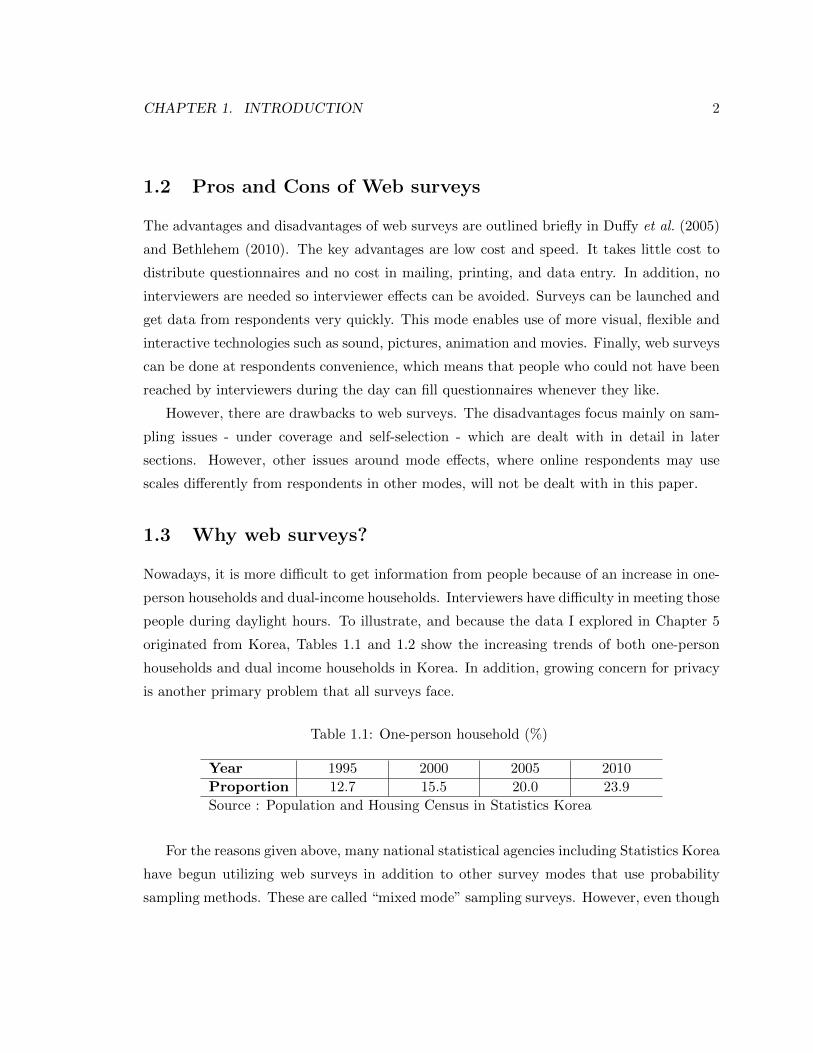
Nowadays, it is more difficult to get information from people because of an increase in one-
person households and dual-income households. Interviewers have difficulty in meeting those
people during daylight hours. To illustrate, and because the data I explored in Chapter 5
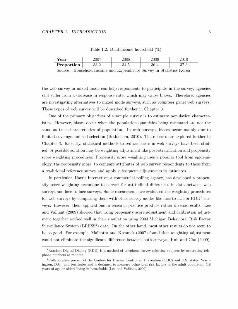
originated from Korea, Tables 1.1 and 1.2 show the increasing trends of both one-person
households and dual income households in Korea. In addition, growing concern for privacy
is another primary problem that all surveys face.
Table 1.1: One-person household (%)
Year 1995 2000 2005 2010
Proportion 12.7 15.5 20.0 23.9
Source : Population and Housing Census in Statistics Korea
For the reasons given above, many national statistical agencies including Statistics Korea
have begun utilizing web surveys in addition to other survey modes that use probability
sampling methods. These are called “mixed mode” sampling surveys. However, even though
CHAPTER 1. INTRODUCTION 3
Table 1.2: Dual-income household (%)
Year 2007 2008 2009 2010
Proportion 33.2 34.5 36.4 37.3
Source : Household Income and Expenditure Survey in Statistics Korea
the web survey in mixed mode can help respondents to participate in the survey, agencies
still suffer from a decrease in response rate, which may cause biases. Therefore, agencies
are investigating alternatives to mixed mode surveys, such as volunteer panel web surveys.
These types of web survey will be described further in Chapter 3.
One of the primary objectives of a sample survey is to estimate population character-
istics. However, biases occur when the population quantities being estimated are not the
same as true characteristics of population. In web surveys, biases occur mainly due to
limited coverage and self-selection (Bethlehem, 2010). These issues are explored further in
Chapter 3. Recently, statistical methods to reduce biases in web surveys have been stud-
ied. A possible solution may be weighting adjustment like post-stratification and propensity
score weighting procedures. Propensity score weighting uses a popular tool from epidemi-
ology, the propensity score, to compare attributes of web survey respondents to those from
a traditional reference survey and apply subsequent adjustments to estimates.
In particular, Harris Interactive, a commercial polling agency, has developed a propen-
sity score weighting technique to correct for attitudinal differences in data between web
surveys and face-to-face surveys. Some researchers have evaluated the weighting procedures
for web surveys by comparing them with other survey modes like face-to-face or RDD1 sur-
veys. However, their applications in research practice produce rather diverse results. Lee
and Valliant (2009) showed that using propensity score adjustment and calibration adjust-
ment together worked well in their simulation using 2003 Michigan Behavioral Risk Factor
Surveillance System (BRFSS2) data. On the other hand, most other results do not seem to
be so good. For example, Malhotra and Krosnick (2007) found that weighting adjustment
could not eliminate the significant difference between both surveys. Huh and Cho (2009),
1Random Digital Dialing (RDD) is a method of telephone survey selecting subjects by generating tele-phone numbers at random
2Collaborative project of the Centers for Disease Control an Prevention (CDC) and U.S. states, Wash-ington, D.C., and territories and is designed to measure behavioral risk factors in the adult population (18years of age or older) living in households (Lee and Valliant, 2009)
CHAPTER 1. INTRODUCTION 4
whose research was supported by Statistics Korea, found similar results in the estimation for
a volunteer panel web survey. According to the paper, the estimates of 79% of 106 variables
showed bias reduction using inverse weights of propensity scores combined with rim weights
for calibration, comparing to unadjusted estimates. However, only 35% of variables showed
more than a 50% reduction in bias.
Nonetheless, I believe that it is worthwhile, even crucial, to investigate web survey
estimation methods further in the future because web surveys are becoming the main data
collection method for its advantages. Lee (2004) argues,
“It becomes the methodologists’ responsibility to devise ways to improve web
survey statistical methods (e.g., sample selection and estimation) and measure-
ment techniques (e.g., questionnaire design and interface usability).”
In this study, bias reduction methods for volunteer panel web surveys will be explored by
comparing face-to-face survey results with web survey results for the Social Survey produced
by Statistics Korea. The methods studied include different variable selection methods for
propensity score calculation and different propensity score weighting methods.
1.4 Outline
The remainder of this study is comprised of the following five chapters. I will review basic
sampling methods and sources of errors in surveys in Chapter 2. Chapter 3 will describe the
web survey types and resulting sampling errors in detail. The core of this study is Chapter
4 and 5. In Chapter 4, I will offer several different approaches to selecting a propensity
score model and discuss methods for using these scores. Propensity score adjustment and
calibration adjustment will be discussed. Adjustment methods include inverse propensity
scores as weights, subclassification (stratification). I will demonstrate these methods on real
data sets originating from Statistics Korea and present results of the analyses in Chapter 5.
Finally, evaluation from the results of the case study and some discussion will be given in
Chapter 6.

Chapter 2
Review of sampling and errors in
surveys
Surveys are conducted to collect information about characteristics of populations. A census
can be done by surveying every unit in the population. However, a sample survey is more
often used because of practical reasons like cost or other constraints. Many well-known
sampling methodologies for conducting statistical inference on sample surveys have been
developed, and many texts and papers have studied and used them. In this chapter, general
sampling methods and sources of errors in surveys are described very briefly to make clear
which sampling methods are possible and what kinds of errors can exist in general surveys.
The next chapter deals with specific sampling methods and problems in statistical inference
for web surveys.
2.1 Concept of sampling
Sampling is the selection of a subset of a larger population to survey. The two broad
categories of sampling methods are probability-based sampling and non-probability sampling
(Fricker, 2008) Probability methods are based on random selection in a variety of ways
from the sample frame of the population. They support the use of statistical techniques for
inferences about the population. In contrast, non-probability sampling is a process where
some elements of the population have no chance of selection or where the probability of
selection can’t be accurately determined. The advantage of non-probability samples is that
5

CHAPTER 2. REVIEW OF SAMPLING AND ERRORS IN SURVEYS 6
they often need much less time and effort. However, the disadvantage is that they may
give biased results because they are not selected randomly (Panacek and Thompson, 2007).
Types of probability sampling include:
• Simple random sampling (SRS): a process in which each subject is selected randomly
from the population with a known and equal probability of being chosen.
• Stratified random sampling: a process in which a population is divided into homoge-
neous subgroups and then random sampling is applied within each group.
• Systematic random sampling: a process in which selection of subjects is conducted
systematically by selecting every nth subject from an ordered sample frame. The
starting point is selected randomly.
• Cluster sampling: a process in which total population is divided into smaller subgroups
(or clusters) and sample is selected by choosing subgroups randomly.
Types of non-probability sampling include:
• Convenience sampling: a process in which a sample is selected from readily available
and convenient subjects. For instance, in volunteer panel web surveys, the use of
self-selection is a kind of convenience sampling.
• Snowball sampling: a process in which the initial subjects are selected in some conve-
nient way and then new subjects are continually recruited based on some connection
to existing subjects.
• Quota sampling: a process in which specified number of subjects for a specific subgroup
are selected in convenient way.
• Purposive sampling: a process in which subjects are selected by the researchers specific
judgment.
Many web surveys are conducted by non-probability sampling methods like convenience
sampling. If a sample is not systematically representative of the population, the resulting
estimates of population quantities may be biased. It is important to try to minimize bias
in this case.

CHAPTER 2. REVIEW OF SAMPLING AND ERRORS IN SURVEYS 7
Figure 2.1: Taxonomy of survey errors, taken from Bethelehem (2010)
2.2 Sources of errors in surveys
The primary purpose of a survey is to estimate population characteristics. However, survey
estimates are not exactly equal to their corresponding population quantities due to various
errors. Bethlehem (2010) presents a taxonomy of survey errors like Figure 2.1 . Those errors
are summarized below.
Total survey error is the difference between a survey-based estimate and the corre-
sponding characteristic of the population. This can be categorized into sampling error and
non-sampling error.
Sampling error occurs due to the fact that some parts of the population cannot be
included in the sample. In other words, it happens that not every subject in the target
population is in the survey. If the whole population can be observed, the sampling errors
disappear. Sampling error can be split into estimation errors and specification errors.
Estimation error occurs because new samples result in different estimates. It is unavoid-
able, but can be quantified by applying probability theory. In the case of web surveys where
samples are drawn by way of self-selection, estimation error occurs but cannot be quantified
since selection probabilities are unknown.
Specification error is due to the difference between true selection probabilities and the

CHAPTER 2. REVIEW OF SAMPLING AND ERRORS IN SURVEYS 8
selection probabilities specified in the sampling design. There is no way to avoid specification
error in the case of web surveys because selection probabilities are unknown as mentioned
before. Therefore self-selection error is a kind of sampling error.
Non-sampling error occurs due to various causes such as data entry error, biased ques-
tionnaires, low response rate and so on. This can be categorized into observation error and
non-observation error.
Observation error occurs when obtaining and recording answers. This can be categorized
into over-coverage error, measurement error and processing error. An over-coverage error
arises because of participation of people who are not in the target population or because of
duplicated participations in the list of sampling units. Measurement error arises when survey
response differs from the true value. It includes the case of respondents misunderstanding
questions, not giving a true answer for sensitive questions, interviewers mistakes and so on.
Processing error means data entry error. Certainly, any of these can occur in web surveys.
Non-observation error means errors caused by omission of intended measurements. This
can be divided into under-coverage error and non-response error. Under-coverage error
occurs when people in the target population cannot be in the sampling frame. This fact
means these people cannot be contacted to participate in a survey. This error can be
common and serious problem for web surveys because, for example, not all members of the
population have Internet access or may find out about the survey. Non-response error is
when selected people do not provide answers to the required questions. This is also common
in web surveys because web surveys are done by self-interviewing. It is obvious that web
surveys can suffer all kinds of errors. However, under-coverage error and sampling error (or
self-selection error) may be the most serious problems in volunteer panel web surveys. This
is described in more detail in the next chapter.

Chapter 3
Web surveys
Web survey mode has become popular for data collection. However, there are drawbacks
to its use in terms of quality of sample estimates because of non-probability sampling and
coverage problems. In this chapter, types of web surveys are described further according
to their sampling methods and main potential problems as discussed in the last chapter.
Volunteer panel web surveys, which are the focus of this paper are described in more detail
than other kinds of web surveys.
3.1 Types of web surveys
“Internet surveys” and “web surveys” are often used interchangeably. However, strictly
speaking, these are different concepts. Web surveys are done only on web browsers, whereas
Internet surveys include both web surveys and surveys which are done by e-mail. Only
web surveys are discussed in this paper. As described before, sampling methods can be
categorized broadly into probability-based sampling and non-probability sampling. Types
of web surveys can also be categorized based on both sampling methods. Table 3.1, which is
a slightly adapted version of Couper (2000), shows the classification of types of web surveys
based on availability of probability sampling. Couper (2000), Lee (2004) and Fricker (2008)
describe characteristics of these kinds of web surveys, which are summarized below.
Web surveys using non-probability sampling methods include entertainment polls, un-
restricted self-selected surveys and volunteer panel surveys.
At first, entertainment polls may not be considered a survey in the scientific sense, but
9

CHAPTER 3. WEB SURVEYS 10
Table 3.1: Types of Web Surveys
Non-probability Probability
1. Entertainment polls 4. Intercept surveys
2. Unrestricted self-selected surveys 5. List-based sample surveys
3. Volunteer panel surveys 6. Web option in mixed mode
7. Pre-recruited panel surveys
they are very popular in many websites. As the name implies, they are mainly done for
entertainment purposes. They consist of websites where any visitor can respond to posted
surveys. There is no control over who responds. One example is question of the day polls
like “CNN Quick vote” (www.cnn.com), which states, “This is not a scientific poll”.
As with entertainment polls, unrestricted self-selected surveys are also open to the public
for anyone to participate in; that is, there are no restrictions on participants. They may
simply be posted on websites or may be prompted via banners. Generally, the distinction
between this type of surveys and entertainment polls is that the latter usually makes few
claims to generalizability, while the former does. Couper (2000) introduced some examples
of this kind of web survey. One is National Geographic Societys “Survey 2000” which
launched in the fall of 1988. An invitation to the survey was posted on its own website and
the URL was published in its magazine. Over 50,000 respondents completed the survey.
In their analysis of the survey results, they note that while the survey did not yield a
random sample and the selection probabilities are unknown, they may yield representative
social science data by estimating the selection probabilities by comparing the distributions
of standard demographic variables to official government statistics and applying weighting,
However, Couper (2000) points out that, in spite of the large sample size, the respondents
of the surveys do not resemble the U.S. population on a number of key indicators due to
self-selection error.
Another example is the web survey “to better understand the risks to adolescent girls
online” which conducted by Berson et al. (2002). The survey was done by posting a link to
their survey on Seventeen Magazine Online website. Over 10,000 responses were collected.
Unlike the first example, the authors were careful to appropriately qualify their results:

CHAPTER 3. WEB SURVEYS 11
“The results highlighted in this paper are intended to explore the relevant issues
and lay the groundwork for future research on youth in cyberspace. This is
considered an exploratory study which introduces the issues and will need to
be supplemented with ongoing research on specific characteristics of risk and
prevention intervention. Furthermore, the generalizability of the study results
to the larger population of adolescent girls needs to be considered. Due to
anonymity of the respondents, one of the limitations of the research design is
the possibility that the survey respondents did not represent the experience of
all adolescent girls or that the responses were exaggerated or misrepresented.”
The results of those kinds of surveys cannot be generalized to a larger population because
researchers do not have any control over the participation mechanism (Lee, 2004). However,
it does not mean that those surveys are useless. As Berson et al. (2002) illustrate, those kinds
of surveys can be helpful in identifying relevant issues for future probability-based surveys.
Furthermore, Fricker (2008) indicates that those kinds of surveys have an advantage in that
they facilitate access to people who are difficult to reach because they are hard to identify
or locate, or perhaps exist in such small numbers that probability-based sampling would be
unlikely to reach them in sufficient numbers.
Volunteer panel web surveys are conducted based on panel lists which consist of people
who decide to participate in continuing surveys via websites. Before surveys, basic demo-
graphic information is collected from those volunteers when they sign up for the registration.
Then, based on the database of the potential respondents, researchers can select panel mem-
bers for a particular survey using sampling procedures like quota sampling or probability
sampling methods according to the volunteers’ demographic information. In this regard,
there is a distinction between this type of web survey and previous ones. However, it is
notable that the initial panel is a self-selected sample of volunteers. This type of web survey
has received much attention within web survey industry recently (Couper, 2000). The web
survey data used for the analysis in this paper were collected using this type, which are
described in detail in Chapter 5. A well-known example of this type is Harris Poll Online.
Harris Interactive says on its website :
“The Harris Poll Online Panel consists of individuals from throughout North
America and Western Europe who have double opted-in and voluntarily agreed

CHAPTER 3. WEB SURVEYS 12
to participate in our various online research studies. Through our careful re-
cruitment, management and incentivized panel members, we are confident that
we have one of the highest quality panels anywhere in the world with sufficient
capacity to provide our clients with the feedback they need to make sound and
compelling business decisions. Top quality panels coupled with deep profiling
of our members allows us to target and accurately survey certain low-incidence,
hard-to-find subjects, rapidly survey large numbers of the general population,
and conduct a broad range of studies across a wide array of industries and
subject-matter sets.”
For this kind of web survey, incentives are often offered to panels to encourage participat-
ing in the surveys. Harris Interactive also offers rewards to their panels. Their key approach
to analysis for the survey is the use of propensity score adjustment for bias reduction, which
is described in Chapter 4. In contrast to previous types of web surveys, probability-based
web surveys begin with probability samples of various forms. Couper (2000) argues that
there are essentially two approaches to achieve probability-based web samples because web
access is not universal and no frame of web users exists. One is to restrict the population
of interest so that the sample is restricted to the web users. The other is to use alternative
methods such as RDD simultaneously in order to identify and reach a broader sample of
the population. Probability-based web survey types include intercept surveys, web option
in mixed mode, and pre-recruited panel surveys.
Intercept surveys are pop-up surveys placed on a specific website that generally use
systematic sampling methods to invite every kth visitor to the site to visit the survey website.
The population in this case is defined as visitors to the site so that this sampling enables
generalization the particular population. Internet Protocol (IP) addresses and cookies1 can
be used to restrict multiple submissions from the same computer user. These surveys seem
to be very useful as customer-satisfaction surveys or site evaluations, but an important issue
with this type of survey is nonresponse (Couper, 2000; Fricker, 2008). Low response rate
may raise nonresponse bias and there may no way to assess it because those who complete
the surveys may have different views compared to those who ignore the request.
Another type of probability-based web survey is a list-based sample survey. The approach
1Cookies are used for an origin website to send state information to a user’s browser and for the browserto return the state information to the origin site.

CHAPTER 3. WEB SURVEYS 13
of this type begins with a frame or list of those with web access. The population is restricted
to the web users. Therefore, this type is typically used for intra-organizational surveys like
student surveys, government organization surveys, and large corporation surveys. There is
little chance of coverage problems in this type of survey. Couper (2000) calls this “list-based
samples of high-coverage populations”. E-mail is usually used to invite participation in the
surveys. Simple random sampling is straightforward to implement and requires only contact
information like e-mail addresses. To implement more complicated sampling methods such
as a stratified sampling more auxiliary information is needed.
Third, pre-recruited panel surveys are similar to volunteer web panel surveys in the
sense of that panels consist of individuals who have agreed to participate in surveys. The
key difference is that the former uses probability sampling methods such as RDD for re-
cruiting panels, while the latter does not. Researchers generally recruit panel members via
telephone or postal mail rather than web or e-mail. After getting information from those
panel members, sub-samples can be drawn by researchers’ specification. If the population
is restricted to the web users, then there is again little chance of coverage errors. In case
the population includes people with no web access, equipment and web access are provided
for corresponding panelists.
A final use of web surveys is as an alternative mode in mixed-mode surveys. Participants
are selected by a probability sampling method and are given the option to complete the
survey using one of several modes, such as web, telephone, mail, or face-to-face. The same
survey is offered in each mode; the use of web mode represents a reduction in cost to the
agency and in burden to the respondent. That is why many national statistical agencies (e.g.
Canada, USA, Korea) have utilized this kind of web survey, as mentioned before. There is
little chance of sampling errors or coverage errors in mixed-mode surveys. However, mode
effects can be an issue in this case, but it is often assumed that they are ignorable. Lee
(2004) argues that, strictly speaking, design-based statistical inferences can be drawn only
under these last four probability-based web surveys.
This paper focuses on volunteer panel web surveys using non-probability sampling meth-
ods. As Lee (2004) suggests, it is not guaranteed that people who respond to a volunteer
panel web survey are representative of the whole target population of the survey. This is
because volunteer panel web survey respondents go through several filtering steps before

CHAPTER 3. WEB SURVEYS 14
Figure 3.1: Volunteer Panel Web Survey Protocol, taken from Lee (2004)
supplying responses to a survey. This is depicted in Figure 3.1 from Lee (2004). It is cer-
tain that web surveys in general may suffer from all kinds of errors described in Chapter
2. In particular, web surveys that use convenience sampling are assumed to have higher
likelihood of generating a biased sample (Fricker, 2008). The main potential is for coverage,
self-selection and non-response errors (Bethlehem, 2010; Lee and Valliant, 2009; Fricker,
2008; Duffy et al., 2005). These problems can occur in volunteer panel web surveys as well.
Specifically, there is a gap between the whole population and the web population. This fact
may cause coverage error. In addition, there are no known selection probabilities during the
recruiting process from the web population. This fact may cause self-selection error, which
was described in Chapter 2 as a kind of sampling error. Finally, there is the possibility of
non-response error during the process of getting answers from respondents. These errors
may combine to cause severe bias in any quantity that is estimated. Consequently, statis-
tical inference for this kind of survey can be of doubtful quality. In the next section, main
potential problems in web surveys are explored in detail.
3.2 Problems in web surveys
3.2.1 Coverage problems
Coverage error occurs when some part of the population cannot be included in the sample
or there are duplicated participants in the list of sampling units. In that case, survey results

CHAPTER 3. WEB SURVEYS 15
are likely to be biased. There are two kinds of coverage error that can occur in web surveys:
under-coverage and over-coverage.
Under-coverage is more common because people who cannot access the Internet cannot
participate in a web survey unless the target population includes only people with Internet.
The possible bias is related not only to the numbers of people who have access to Internet,
but also to the difference among them in age, gender, education and behavioral character-
istics Steinmetz et al. (2009). As Bethlehem (2010) mentions, it is well known that young
people and those with high levels of education more often have access to the Internet than
elderly people and those with low levels of education. If some demographic2 groups are
under-represented, this may cause bias problems for inference.
It is worth noting that other modes like computer-assisted telephone survey suffer from
this coverage problem when telephone directories are used as a sampling frame, because peo-
ple without phones or who have unlisted numbers will be excluded from the survey. Surveys
are not generally welcome on cell phones, so current technology changes may exacerbate this
problem. Considering the rapid increase of Internet penetration rates in developed countries
as shown in the Chapter 1, under-coverage problems with web surveys may decrease in the
future.
Over-coverage for web surveys may occur when people participate in surveys multiple
times because of incentives. This happens because it is common that people have multiple
e-mail addresses. It is difficult to identify individual respondents in a web survey. Therefore,
there is usually a possibility of over-coverage problem in web survey. However, it is often
assumed that this problem is not too severe.
3.2.2 Selection problems in web surveys
Non-probability sampling methods, such as convenience sampling, are dominant in web
surveys because of their ease and cost. As described before, this fact causes sampling
errors including estimation and specification error. Horvitz and Thompson (1952) show
that unbiased estimates can be computed only when a real probability sample is used, every
unit in the population has a non-zero probability of selection, and all these probabilities are
known to the researchers. In addition, the precision of estimates can be estimated under
these conditions. However, self-selection surveys do not satisfy these conditions.
2age, sex, racial origin, education

CHAPTER 3. WEB SURVEYS 16
It is also known that people who self-select into a survey differ from those who do not in
terms of time availability, web skills or willingness to contribute to the project (Steinmetz
et al., 2009). In other words, the people who participate in volunteer web surveys may
have specific characteristics. Consequently, their responses may differ substantially from
those of people randomly chosen in the general population. Loosveldt and Sonck (2008)
introduced some previous research to study this selectivity bias by comparing self-selection
web surveys and telephone surveys or face-to-face surveys3. For example, Duffy et al.
(2005) compared web volunteer panel surveys and face-to-face surveys that use probability
sampling. They showed that web survey respondents were more socio-politically active than
those responding to a face-to-face survey. Vehovar et al. (1999) found differences between
web respondents and telephone survey respondents with frequent Internet access in four of
the seven items concerning electronic trade largely due to different experience between two
samples. Bandilla et al. (2003) also observed significant differences between responses of
Internet users and those of mail survey respondents taken by self-interviewing, even after
adjusting the sample of Internet users for basic socio-demographic characteristics.
Theoretically, there are no unbiased estimators in volunteer panel web survey using self-
selection in sampling (Bethlehem, 2010). Therefore, strong structural assumptions must
hold for valid inference (Lee, 2004). These assumptions will be dealt with in detail in
Chapter 4.
3.2.3 Non-response problems
Non-response error occurs when people in a sample do not provide some required informa-
tion. Non-response may be serious problem if answers are significantly different between
respondents and non-respondents. The extent of non-response bias depends on both non-
response rate and difference between respondents and non-respondents (Steinmetz et al.,
2009).
Non-response bias is not unique to web surveys. However, response rates in web surveys
tend to be lower than other modes. Lozar et al. (2008) found that non-response rates of the
3An interviewer is physically present to ask the survey questions and to assist the respondent in answeringthem

CHAPTER 3. WEB SURVEYS 17
web mode is on average 11% lower than those of other modes. Steinmetz et al. (2009) sum-
marized the reasons for this: inefficiency of response-stimulating efforts (incentives, follow-
up contacts), technical difficulties (slow, unreliable connections, low-end browsers), personal
computer accessibility, and privacy and confidentiality concerns. For a non-probability web
survey like a volunteer panel web survey, it is impossible to compute an exact non-response
rate because selection probabilities are unknown.
Even though non-response bias can be a serious problem in web surveys, it is hard to
detect the effect of it. In this paper, non-response will be assumed to be missing at random
(MAR4). The imputation method for missing data that I applied to data sets is described
briefly in Chapter 5.
4Missing data are partly caused by an auxiliary variable X. If there is a relationship between this variableX and the target variable Y , estimates for Y will be biased. But it can be corrected by a technique thatuses the distribution of X in the sample.

Chapter 4
Methodology
As described above, bias can be caused by a variety of sources of errors. In order to reduce
bias, the data can be adjusted to correct those errors. Weighting adjustments are techniques
that attempt to improve the accuracy of survey estimates by using auxiliary information
(Bethlehem, 2010). They are considered possible solutions to improve quality in web sur-
veys. Weighting adjustment methods include post-stratification weighting, propensity score
adjustment, and rim weighting adjustment (Lee, 2004; Bethlehem, 2010; Steinmetz et al.,
2009; Looseveldt and Sonck, 2008; Huh and Cho, 2009).
Post-stratification is a calibration estimation method to reduce the variance of the esti-
mates and reduce bias due to non-coverage and non-response (Cervantes et al., 2009). It is
used to adjust for demographic differences between a sample and the population. Looseveldt
and Sonck (2008) argue that the method does not solve the problem of selection bias since
some response variables may be related to variables other than demographics. For example,
attitudinal and behavioral differences can be observed even after applying post-stratification
weighting adjustment using demographic variables. Post-stratification is described further
in Section 4.1.
As an alternative, propensity score adjustment has been applied to volunteer panel web
surveys. The technique is primarily used in the context of observational studies (e.g., Rosen-
baum and Rubin (1983)). The idea is to make two samples comparable by weighting using
all auxiliary variables that are thought to account for the differences. In context of web sur-
veys, this technique aims to correct for differences between online people and offline people,
which were caused by certain inclinations of people who participate in a volunteer panel
web survey. In order to do that, a reference survey based on probability sampling is needed
18

CHAPTER 4. METHODOLOGY 19
Figure 4.1: Proposed Adjustment Procedure for Volunteer Panel Web Surveys, taken fromLee (2004)
and is assumed to produce unbiased estimates (Bethlehem and Stoop, 2007). Propensity
score adjustment using a reference survey is described further in Section 4.2.
Lee and Valliant (2009) suggest the combination of propensity score adjustment and
calibration adjustment to reduce bias caused by nonrandomized sample selection and de-
ficient coverage in volunteer panel web surveys. Figure 4.1 shows the proposed procedure
for the surveys. Propensity score adjustment is used to make the web sample behave like
the reference sample, calibration is used to make the reference sample represent the popula-
tion. Calibration can be used to correct both non-response and coverage errors that are not
controlled by the propensity score adjustment. Several calibration methods exist such as
generalized regression estimators (GREG) and rim weighting. We use rim weighting which
is described in detail in Section 4.3.
4.1 Post-stratification
It is important to have a representative sample of the population when conducting a survey.
However, cases of not having such a sample often occur accidentally or intentionally. For
example, the distribution of a certain characteristic such as age, education, race, or gen-
der (so-called demographic variables) in a sample may differ from the distribution in the
population. This gives rise to potential bias if responses are related to the demographic

CHAPTER 4. METHODOLOGY 20
variables, because statistical procedures will give greater weight to oversampled people.
Post-stratification survey weighting corrects for this bias mathematically. The basic idea
is to stratify the sample into a number of cells, based on characteristics of the population
deemed important, and then to give more weight to respondents in under-represented groups
and less weight to those in over-represented groups.
Steinmetz et al. (2009) suggest a formula for post-stratification weights in web surveys.
The formula can be used for one or more demographic variables based on the cell proportions
from contingency tables of those variables for both the sample and the target population.
The weight wi for an element i in stratum (i.e., cell) h is equal to
wi =Nh/N
nh/n,
where N is the number of target population elements, Nh is the number of target population
elements in stratum h, n is the sample size, and nh is the sample size in stratum h. Identical
weights are assigned to all elements in the same stratum. Note that this approach can be
applied only when the population proportions in each stratum are available. Therefore, this
approach is not applied in this study, because the population proportions were not available
for many of the variables in my data.
4.2 Propensity Score Adjustment (PSA)
The original propensity score adjustment was suggested by Rosenbaum and Rubin (1983,
1984) for the purpose of the comparison of populations in the context of observational stud-
ies. For example, in observational studies where assignment of the study subjects to the two
groups (e.g., treatment and control groups) is not random, the probability that a randomly
selected subject with a given set of covariates would be in the treatment group rather than
the control group is defined as that subject’s “propensity” for treatment. Propensity scores
are estimated for each subject, and then a treated case is matched to a control case or sub-
classified based on closeness of propensity score in order to estimate the difference in means
for the two groups (Lee, 2004). Harris Interactive, a commercial polling company, is the first
agency known to have applied this method in order to estimate population characteristics
in the context of web surveys.

CHAPTER 4. METHODOLOGY 21
4.2.1 Reference surveys
In order to conduct propensity score adjustment in the context of web surveys, a reference
survey is needed which represents the control group (Lee, 2004). It is assumed that the
reference survey produces unbiased estimates (Bethlehem and Stoop, 2007). For instance,
the reference survey may be conducted by using a traditional survey mode, such as RDD
in Harris Interactive’s case. A reference survey can be an existing survey or a smaller scale
survey that collects data closely related to the web surveys. Variables which are included
both the reference survey and the web survey can be used as covariates for predicting
whether a randomly selected respondent participated in the web survey or the reference
survey.
As described before, demographic variables can be used for correcting unrepresenta-
tiveness of web surveys with respect only to those variables. In order to further reduce
self-selection bias in web surveys, some other variables to capture the differences between
the online and offline populations are needed (Schonlau et al., 2007). Questions designed
for this purpose are diversely called webographic, attitudinal or lifestyle questions. Harris
Interactive introduced webographic questions which consist of attitudinal questions, factual
questions and privacy questions (Schonlau et al., 2007). Table 4.1 shows all the questions
used by Harris Interactive.
Lee (2004) uses attitudinal questions like self-rated social class, employment status,
political party affiliation, having a religion, and opinion toward ethnic minorities as variables
for propensity scoring. In this paper, the term “webographic variables” is used later for the
above concepts.
4.2.2 Propensity score
A propensity score is simply the probability of a unit i (i = 1, . . . , n) being assigned to the
treatment group (zi = 1) given a set of covariates (xi) and is denoted as
e(xi) = Pr(zi = 1|xi), (4.1)
where it is assumed that zi are independent given a set of covariates (xi), and e(xi) ranges
from 0 to 1.
“Treatment” means being in a web survey in the web survey context. In other words, a
propensity score is the conditional probability that a person will be in a web survey rather

CHAPTER 4. METHODOLOGY 22
Table 4.1: Webographic Questions by Harris Interactive
Attitudinal variablesDo you often feel alone? (yes/no)
Are you eager to learn new things? (yes/no)
Do you take chances? (yes/no)
Factual variablesIn the last month have you traveled? (yes/no)
In the last month have you participated in a team or indi-vidual sport? (yes/no)
In the last month have you read a book? (yes/no)
Privacy Variables
Which of these practices, if any, do you consider to be aserious violation of privacy?
Please check all that apply.
1. Thorough searches at airport checkpoints, based on visualprofiles
2. The use of programs such as ’cookies’ to track what anindividual does on the Internet
3. Unsolicited phone calls for the purpose of selling productsor services
4. Screening of employees for AIDS
5. Electronic storage of credit card numbers by Internetstores
Lifestyle variables
Do you know anyone who is gay, lesbian, bisexual, ortransgender?
Please check all that apply.
1. Yes, a family member
2. Yes, a close personal friend
3. Yes, a co-worker
4. Yes, a friend or acquaintance (not a co-worker)
5. Yes, another person not mentioned
6. No

CHAPTER 4. METHODOLOGY 23
than in a reference survey given a set of observed covariates (Steinmetz et al., 2009). In
addition, the propensity score is a balancing score which has the property that treatment
assignment is conditionally independent of the covariates given the balancing score (Lee,
2004). This means respondents in both surveys with the same propensity score have the
same distribution of x (Schonlau et al., 2007). It can be expressed mathematically as
x ⊥ z|b(x),
where b(x) is the balancing score.
Moreover, Lee (2004) also shows that in theory the adjustment based on a propensity
score leads to an unbiased estimate of treatment effect, i.e., the difference between web and
reference survey mean, as long as certain assumptions hold. The assumptions are described
in the next subsection.
The aim of propensity score adjustment is to enable a form of post-stratification so that
estimates of variables of interest for the web sample are similar to those for the reference
sample within each group of approximately equal propensity scores. Modeling and some
methods for the propensity score adjustment are described in detail in the Subsection 4.2.4
and 4.2.5.
4.2.3 Assumptions in propensity score adjustment
Lee (2004) outlines five assumptions in observational studies in order that propensity score
adjustment should be valid for bias reduction and adapt these meanings to apply to web
surveys. These are summarized below.
First, any propensity score should meet the ‘strong ignorability assumption’:
Y ⊥ z|e(x) and 0 < Pr(z = 1|e(x)) < 1,
where Y is the response variable. In case of randomized treatment assignment, this assump-
tion holds and adjustments based on the propensity scores produce the unbiased estimates.
However, in case of nonrandomized treatment assignment, this is not necessary true. There-
fore, this assumption is critical in web surveys using convenience sampling methods. Strong
ignorability implies that there are no unobserved variables that explain selectivity into the
web sample and that are also related to the question of interest Y (Schonlau et al., 2007).
In volunteer panel web surveys, strong ignorability could be violated if some important co-
variates in propensity score modeling are omitted or responses are related to covariates that
CHAPTER 4. METHODOLOGY 24
are not used.
The second assumption is no contamination among study units which means that a
treatment assigned to one unit does not affect the outcome for any other unit. Third, any
unit must be assigned to either treatment or control for any configuration of x. Fourth, the
observed covariates included in propensity score models represent the unobserved covari-
ates, because balance is not necessarily achieved on unobserved covariates. If an important
covariate, e.g., education, was omitted from the model and the web sample subjects and
non-web sample subjects had different distributions of levels of education, then this assump-
tion would be violated. The last assumption is that the assigned treatment does not affect
covariates. None of them can be altered by a person’s participation in one or the other
survey.
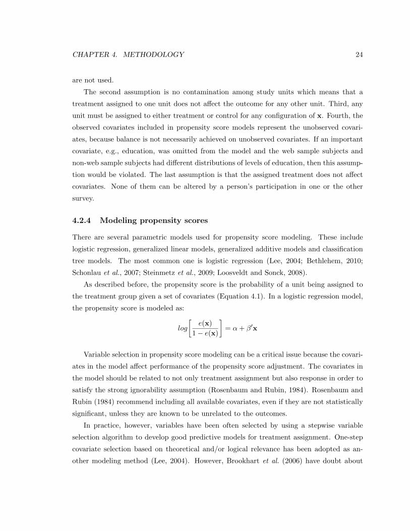
4.2.4 Modeling propensity scores
There are several parametric models used for propensity score modeling. These include
logistic regression, generalized linear models, generalized additive models and classification
tree models. The most common one is logistic regression (Lee, 2004; Bethlehem, 2010;
Schonlau et al., 2007; Steinmetz et al., 2009; Loosveldt and Sonck, 2008).
As described before, the propensity score is the probability of a unit being assigned to
the treatment group given a set of covariates (Equation 4.1). In a logistic regression model,
the propensity score is modeled as:
log
[e(x)
1− e(x)
]= α+ β′x
Variable selection in propensity score modeling can be a critical issue because the covari-
ates in the model affect performance of the propensity score adjustment. The covariates in
the model should be related to not only treatment assignment but also response in order to
satisfy the strong ignorability assumption (Rosenbaum and Rubin, 1984). Rosenbaum and
Rubin (1984) recommend including all available covariates, even if they are not statistically
significant, unless they are known to be unrelated to the outcomes.
In practice, however, variables have been often selected by using a stepwise variable
selection algorithm to develop good predictive models for treatment assignment. One-step
covariate selection based on theoretical and/or logical relevance has been adopted as an-
other modeling method (Lee, 2004). However, Brookhart et al. (2006) have doubt about

CHAPTER 4. METHODOLOGY 25
effectiveness of this kind of variable selection method. They use a simulation study to show
that variables that are unrelated to the treatment assignment but related to the response
should always be included in a propensity model.
In many previous studies for evaluation of propensity score adjustment in web surveys,
variable selection was conducted in such a way that models included all covariates, of which
numbers range from 5 to 30 (e.g., Lee and Valliant, 2009; Bethlehem, 2010; Schonlau et al.,
2007; Steinmetz et al., 2009; Loosveldt and Sonck, 2008). In fact, in most of these studies,
the numbers of available variables in both web and web survey are within around 10. How-
ever, there is a limit on the number of covariates in models because those variables should
be included in both web and reference surveys and it is difficult to recruit participants to
complete very long surveys.
Lee and Valliant (2009) compare five different logistic models in order to separately
examine effects of stratifying variables (age, gender, education, and race) and webographic
variables. The base model (Model 2) includes all available 30 covariates. Models 1, 3, 4
and 5 use subsets of the covariates in Model 2. In order to test the role of significance
testing, covariates roughly with p-value ≤ 0.2 are used in Model 3. In order to detect
the marginal effect of stratifying variables used in their simulation, Model 1, 4 and 5 are
constructed. Model 1 includes only the stratifying variables. Model 4 uses all variables
except the stratifying variables. Model 5 includes significant covariates at the 0.2 level but
excludes the stratifiers. The results of the study shows that Model 2 and 3 appear to produce
reasonable bias reduction across all covariates. Huh and Cho (2009) use 9 or 7 covariates
in their model out of 123 available covariates suggesting that some guidelines should be
considered in selecting webographic variables, which include:
• Questions should be ‘fundamental’ so that the answers would not be changed easily.
For example, people would not change their opinions regarding a ‘fundamental’ ques-
tion asking about ‘the necessity of unification of Korea’, while the opinions regarding
the ‘necessity of the six-party talks1’ can be changed easily by the political situations
when the survey is taken.
• Questions should be easy to be answered in order to minimize measurement error
1The six-party talks aim to find a peaceful resolution to the security concerns as a result of the NorthKorean nuclear weapons program. There has been a series of meetings with six participating states: SouthKorea, North Korea, China, USA, Russia, Japan.

CHAPTER 4. METHODOLOGY 26
because hard ones have room for severe measurement errors.
• Questions should distinguish well between a web and a reference group participating
in a survey.
This approach may be reasonable. However, there seems to be room for criticism that
it can be subjective, because different people can select different questions as webographic
variables if there are not enough studies of the questions.
For the best performance of propensity score adjustment, selecting covariates for each
model corresponding to each response variable seems be important in order to meet the
strong ignorability assumption. However, this approach seems to be impractical in web
surveys, even impossible for large surveys. The number of available response variables and
covariates in data sets used in this paper, which will be described in Chapter 5, is over
100. Constructing a separate propensity score model for each response variable, which
may generate as many models as there are response variables in worst case, is not feasible.
Therefore, it is important to select an acceptable number of webographic variables that
work broadly with many responses for use in future surveys. As Lee (2004) mentions, there
seem to be no clear-cut criteria for selecting variables for propensity score model building.
It is hard to define what kind of questions could be used as webographic variables.
In this paper, some possible variable selection methods are explored, which include step-
wise based on information criteria, and ‘Least Absolute Shrinkage and Selection Operator’
(LASSO) selection in a logistic regression model, and boosted tree models.
Stepwise techniques (including forward and backward selection) have been used as au-
tomated procedures (e.g., SAS PROC GLM or LOGISTIC) for regression analysis. They
are summarized briefly below.
• Forward selection begins with null model and adds the most significant variable to the
model one at a time until there are no variables that meet a stated criterion.
• Backward selection begins with full model and removes the least significant variable
one at each step until there are no variables that meet a stated criterion
• Stepwise selection combines the elements of the previous two.
In particular, Shtatland et al. (2008) suggest the combination of stepwise logistic regres-
sion, information criteria, and best subset selection using SAS PROC LOGISTIC instead

CHAPTER 4. METHODOLOGY 27
of ordinary stepwise selection if the goal of modeling is prediction, when there is a large
number of covariates and little theoretical guidance for choosing among them. The basic
idea behind the information criteria is penalizing the likelihood for the model complexity.
Akaike information criterion (AIC) and Schwarz’s criterion (SIC2) are most popular. The
general form is
IC(c) = −2logL(M) + c ∗K,
where logL(M) is the maximized log likelihood for the fitted model, N is the sample size,
K is the number of covariates, and c is a penalizing parameter. The AIC and SIC can be
defined as information criteria with c=2 and c = logN correspondingly. The first step for
this approach is to use the stepwise selection method with significance level to enter and
significance level to stay close to 1 (e.g., significance level to enter =0.99 and significance
level to stay =0.995) in order to get a sequence of models starting with the null model and
ending with the full model. Then, we can choose the model which has the smallest value of
the information criteria.
Another technique of variable selection is LASSO selection. The LASSO parameter
estimates are given by
βlasso = argminβ
n∑i=1
(yi −p∑j=1
xijβj)2
subject top∑j=1
|βj | ≤ s,
where n is sample size, yi are values of the dependent variable, xij are the values of the
predictor variables, and s is a shrinkage factor. The LASSO method can be used in SAS
PROC GLMSELECT, which was originally developed in the context of linear models as fit
by PROC GLM. However, it has been applied with binomial logistic as well (Roth, 2004).
Finally, classification tree modeling can be used. Classification tree is used for determin-
ing a set of split conditions that permit accurate classification of cases. Roe et al. (2005)
indicate that classification trees are powerful, but unstable because a small change in the
training data can produce a large change in the tree, so boosting can be a remedy. Boosting
is based on the observation that finding many rough rules of thumb can be a lot easier than
2Also known as Bayseian information criterion (BIC) or Schwarz’s Bayseian criterion (SBC), or Schwarz’scriterion(SC)

CHAPTER 4. METHODOLOGY 28
finding a single, highly accurate prediction rule. Boosting can produce a very accurate pre-
diction rule by combining rough rules via iterative algorithms (e.g., AdaBoost algorithm).
Variables can be selected according to “relative influence” values (Elith et al., 2008). The
relative influence of each variable is scaled so that the sum adds to 100, with higher numbers
indicating stronger influence on the response. A disadvantage of this approach is computa-
tional burden. In case of large numbers of categorical variables with many categories, the
computations performed may require an unreasonable amount of effort and time. The the-
ory of this method is not discussed in detail in this paper. The R package “gbm” (General
Boosted Model) provides boosted classification tree modeling method.
Applications of those above three modeling methods are described and compared in
Chapter 5. As described above, modeling for propensity score adjustment can be critical
for its effectiveness. In addition, the number of covariates in the model can be important
in terms of practice because few researchers would want to use those large complex models
just for computing propensity scores.
4.2.5 Applyng methods for propensity score adjustment
D’Agostino (1998) introduces three propensity score adjustment methods: matching, sub-
classification (also called stratification) and regression adjustment. Matching is very popular
in observational studies where there are a limited number of treated group members, and
a larger number of control group members. Members of one sample are paired with mem-
bers of the other sample according to their propensity scores. Then methods for estimating
treatment differences using paired data are applied to the response variable. However, in
the context of web surveys, pair matching has a limitation, because the response variable
is typically measured only in the web surveys (Lee, 2004). The author also indicates that
regression adjustment is not as widely applied as subclassification or matching because of
poor performance. Therefore, the above two methods are not dealt with in this paper. In-
stead, using inverse propensity scores as weights is described as an alternative, along with
subclassification. With both techniques, the propensity score is calculated the same way,
but once it is estimated it is applied differently.

CHAPTER 4. METHODOLOGY 29
Inverse propensity scores as weights
This approach is the simplest method. Recall that a propensity score is the conditional
probability that a person will be ‘in a web survey’ rather than ‘in a reference survey’ given
a set of observed covariates, that is
e(xi) = Pr(zi = 1|xi)
where zi is an indicator variable for membership in the web survey, and xi are covariates in
the model.
After calculating the propensity scores, weights (wpsi ) of web survey are formed as the
inverse of the propensity scores (Steinmetz, 2009):
wpsi =1
e(xi)
Those weights can then be multiplied with base weights such as sampling weights (if
applicable, e.g., in case that subjects of web survey are chosen from the pool of volunteers
by probability-based sampling) for the final weights. Note that survey weights are not used
in developing the propensity score model. Hahs-Vaughn and Onwuegbuzie (2006) state that
this is not necessary because propensity scores are used only to form subclasses with similar
background covariates, not to make inferences about the population-level propensity score
model.
Subclassification (Stratification)
Subclassification is commonly used in observational studies to identify systematic differences
between the treated and control groups. Harris Interactive and Lee and Valliant (2009)
applied this approach to their web survey studies. Lee and Valliant (2009) describe the
process of applying this approach, which is summarized below.
Denote the volunteer panel web survey sample as sW with nW units, each with a base
weight of dWj , where j=1, . . . , nW , and the reference survey sample as sR with nR units,
each with a base weight of dRk , where k=1, . . . , nR. Base weights can be sampling weights
from larger panel in the web survey or population in the reference survey. We can set dWj
and dRk as 1 if no base weights are already given in the both surveys. First, the two samples
are combined into one, s = (sW ∪ sR), with n = nW + nR units. After estimating each

CHAPTER 4. METHODOLOGY 30
propensity score from the combined sample (e(xi) = Pr(i ∈ sW |xi), i = 1, . . . , n), those
units (s) are partitioned into C subclasses according to ordered values of e(xi), where each
subclass has about the same number of units. In the cth subclass in the merged data,
denoted as sc, there are nc = nWc + nRc units, where nWc is the number of units from the
web survey data and nRc is the number of units from the reference survey. Total number of
units in the combined data reamains the same :
C∑c=1
(nWc + nRc ) =
C∑c=1
(nc) = n.
Then, compute the following adjustment factor that will be applied to all units in the
cth subclass of the web survey data (sWc ):
fc =
∑k∈(sRc ) d
Rk /∑
k∈(sR) dRk∑
j∈(sWc ) dWj /∑
j∈(sW ) dWj
, (4.2)
where sRc and sWc are the sets of units in the reference sample and web sample, respectively,
of the cth subclass. If the base weights in equation (4.2) are the inverses of selection
probabilities, the adjustment is equivalent to
fc ≡NRc /N
R
NWc /NW
,
where N lc =
∑k∈(slc) d
lk is the estimated population count of units based on the reference or
web survey (l = R or W ) and Nl =∑
C Nlc. The propensity score adjusted (PSA) weights
for unit j in sWc is
dW.PSAj = fcdWj =
∑k∈(sRc ) d
Rk /∑
k∈(sR) dRk∑
j∈(sWc ) dWj /∑
j∈(sW ) dWj
dWj .
If the base weights are equal for all units or are not available, an alternative adjustment
factor can be used, which is
fc ≡nRc /n
R
nWc /nW.
Finally, the estimator for the mean of a study variable, y, for the web survey sample is
ˆyW.PSA =
∑c
∑j∈(sWc ) d
W.PSAj yj∑
c
∑j∈(sWc ) d
W.PSAj
.
CHAPTER 4. METHODOLOGY 31
It is notable that the reference sample is required to have only the covariate data, not
necessarily the variables of interest. This is because the reference sample units are not used
in in computing ˆyW.PSA after adjustment weights are calculated. Finally, it is assumed that
mode effects between web and reference survey can be disregarded.
It is possible to create numerous subclasses assuming that more homogeneous groups may
be partitioned into each subclass. However, the possibility of no inclusion of either treated
group or control group within subclasses increases as the number of subclasses increases.
Since Cochran (1968) found that five subclasses are often sufficient to remove over 90 percent
of the bias, many researchers use the quintiles of the estimated propensity score from the
combined group to determine the cut-offs for the different subclass (D’Agostino, 1998).
Subclassification is popular because it has some advantages, which include (1) it is easier
than matching, (2) the number of control group subjects need not be larger than that of
the treated group, and (3) subclassification uses all subjects, whereas matching discards
unmatched subjects (Lee, 2004).
4.3 Calibration (Rim weighting)
Propensity score adjustment makes response estimates in a web survey resemble those hy-
pothetically taken in a probability-based reference survey. As discussed before, Lee and
Valliant (2009) suggest a second stage adjustment to make the propensity-score-adjusted
web survey sample resemble the target population. One such method of adjustment is called
rim weighting.
Rim weighting was originally developed by Deming and Stephan (1940) in order to en-
sure that complete census data and samples taken from it gave consistent results. The
method matches sample and population characteristics only with respect to the marginal
distributions of selected covariates, while post-stratification needs the joint distributions of
the covariates, which is often not available for the population. Rim weighting can be con-
ducted by an iterative algorithm to alternately adjust weights according to each covariates’
marginal distribution until convergence. There are many algorithms for doing this. The one
below is developed by Little and Wu (1991).
Consider two discrete covariates, with I and J levels, respectively, and suppose that the
sample frequencies are laid out in an I×J contingency table. Let nij be the cell count in ith
row and jth column, n = total counts, and let wi and wj be the target marginal proportions

CHAPTER 4. METHODOLOGY 32
of row i and column j in population, respectively.
1. Initialize the weights by setting each equal to w(0)ij =
nijn
.
2. Raking over rows : w(1)ij = wi ×
w(0)ij∑i w
(0)i
.
3. Raking over columns : w(2)ij = wj ×
w(1)ij∑i w
(1)j
.
4. Repeat step 2 and 3 until∑
j wij = wi and∑
i wij = wj for each i and j, i.e.,
convergence is achieved.
If the sample sizes in each cell are large enough, the raking estimator is approximately
unbiased. However, a disadvantage of rim weighting is that the algorithm may be slow
and even not converge if some of the cell estimates are zero. Huh and Cho (2009) indicate
that rim weighting can be used in sampling methods such as systematic sampling from the
weighted list. The sampling from the pool of all volunteers for the web survey in the case
study for this paper was done by this method.

Chapter 5
Case Study
This chapter explores the performance of the proposed adjustment approaches for volunteer
web panel surveys presented in Chapter 4. The purpose of the adjustment approaches is to
reduce bias that may occur from the non-probability sampling and under-coverage errors.
The web survey and reference survey data used in this study were provided by Statistics
Korea. The effects of propensity score models, PSA methods and calibration adjustment
are compared in order to examine the degree of bias reduction associated with each.
5.1 Data
In 2009 Statistics Korea conducted a web survey to evaluate statistical estimation methods
like propensity score adjustment and rim weighting for volunteer panel web surveys. Some
of the questions from the 2009 Social Survey (reference survey) were included in the web
survey questionnaire. Huh and Cho (2009) performed an analysis of the results based on the
data sets. The data sets are used in this paper as well, but methods are applied differently.
The main differences are summarized in Table 5.1.
5.1.1 Reference survey data
The Social Survey consists of total 10 areas biennially. The 2009 survey included sections on
Welfare, Culture & Leisure, Income & Consumption, Labor, and Social Participation. The
2010 survey included Family, Education, Health, Environment, and Safety. The 2009 sur-
vey, used in this study, sampled all persons aged 15 and over who normally reside in 17,000
33

CHAPTER 5. CASE STUDY 34
Table 5.1: The main differences between Huh & Cho (2009) and this study
Huh and Cho (2009) This study
Model - Model selection and - Data splitting : Training
selection evaluation for all data data for model selection
and and Test data for evaluation.
evaluation - 9 or 7 variables in the model - LASSO, Stepwise based on
considering some guidelines information criteria, Boosted
(see the Subsection 4.2.4). tree.
- Imputation for those - Imputation for all covariates
covariates in the model except over 50% nonresponse
and complete data rate.
analysis without
nonresponse variables.
propensity score - Inverse propensity scores as - Inverse propensity scores as
adjustment weights. weights and subclassification.
selected households during the survey period. A total of 37,049 respondents participated
in the survey. This survey was conducted face-to-face. For estimation, post-stratification
weights are calculated based on population characteristics by gender, age and area of res-
idence. This survey plays the role of reference survey in this study, and the estimates of
responses are assumed to be true values of the population for evaluation of bias in this
survey.
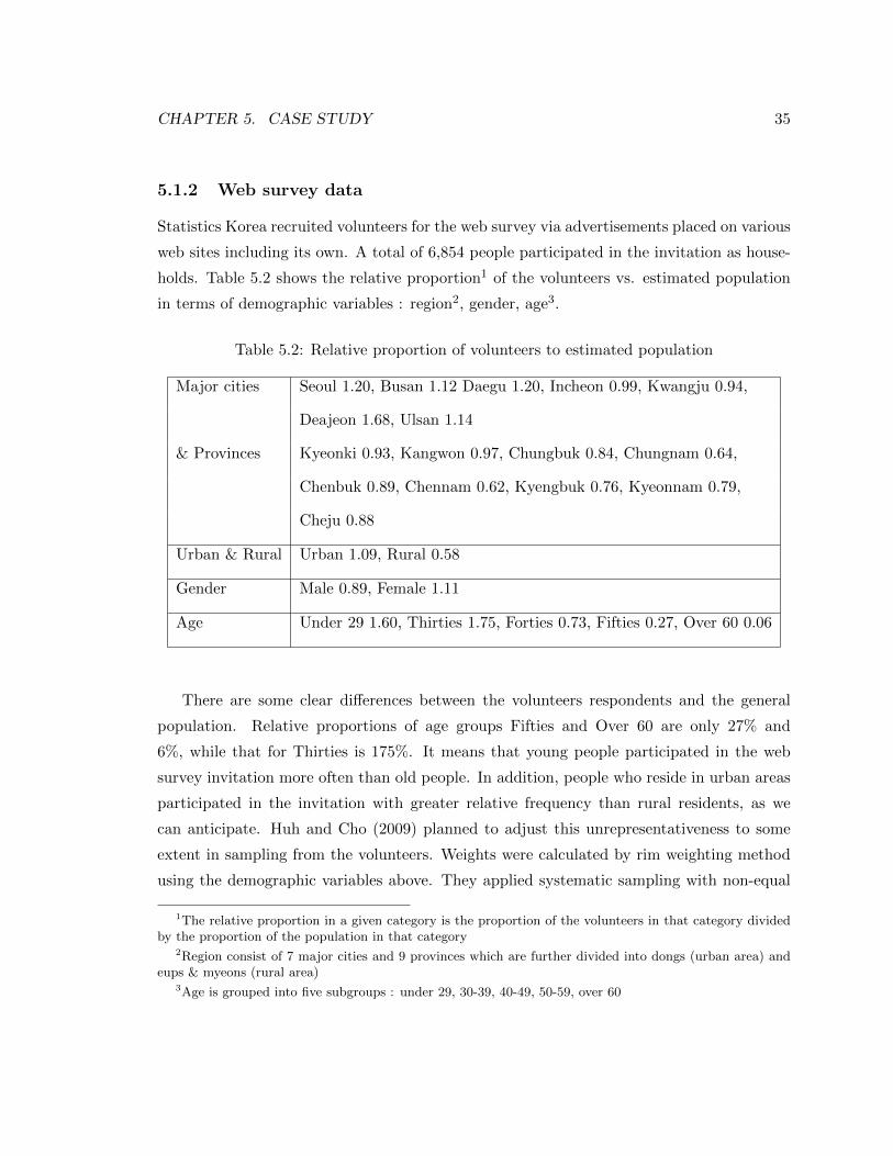
CHAPTER 5. CASE STUDY 35
5.1.2 Web survey data
Statistics Korea recruited volunteers for the web survey via advertisements placed on various
web sites including its own. A total of 6,854 people participated in the invitation as house-
holds. Table 5.2 shows the relative proportion1 of the volunteers vs. estimated population
in terms of demographic variables : region2, gender, age3.
Table 5.2: Relative proportion of volunteers to estimated population
Major cities Seoul 1.20, Busan 1.12 Daegu 1.20, Incheon 0.99, Kwangju 0.94,
Deajeon 1.68, Ulsan 1.14
& Provinces Kyeonki 0.93, Kangwon 0.97, Chungbuk 0.84, Chungnam 0.64,
Chenbuk 0.89, Chennam 0.62, Kyengbuk 0.76, Kyeonnam 0.79,
Cheju 0.88
Urban & Rural Urban 1.09, Rural 0.58
Gender Male 0.89, Female 1.11
Age Under 29 1.60, Thirties 1.75, Forties 0.73, Fifties 0.27, Over 60 0.06
There are some clear differences between the volunteers respondents and the general
population. Relative proportions of age groups Fifties and Over 60 are only 27% and
6%, while that for Thirties is 175%. It means that young people participated in the web
survey invitation more often than old people. In addition, people who reside in urban areas
participated in the invitation with greater relative frequency than rural residents, as we
can anticipate. Huh and Cho (2009) planned to adjust this unrepresentativeness to some
extent in sampling from the volunteers. Weights were calculated by rim weighting method
using the demographic variables above. They applied systematic sampling with non-equal
1The relative proportion in a given category is the proportion of the volunteers in that category dividedby the proportion of the population in that category
2Region consist of 7 major cities and 9 provinces which are further divided into dongs (urban area) andeups & myeons (rural area)
3Age is grouped into five subgroups : under 29, 30-39, 40-49, 50-59, over 60

CHAPTER 5. CASE STUDY 36
selection probabilities equal to the inverse of the weights. A total of 1,500 households were
chosen as the sample, the size of which was related to the budget for incentives. Table 5.3
shows relative proportions of the sample to the estimated population. According to the
Table 5.3, the relative proportions of the sample were improved compared to those of the
all volunteers. For example, relative proportions of age groups of Fifties and Over 60 were
improved to 107% and 29% from 27% and 6%, respectively. The relative proportion of rural
area was improved to 85% from 58%. Huh and Cho (2009) state that the difference left
after sampling happened because they prevented too much weighting of a small number of
subjects by setting an upper limit on weights at five, and that it can be adjusted by further
propensity score and rim weighting. In all, a total of 2,903 respondents, who reside in the
1,500 households, participated in the web survey. The number of overlapping covariates
between the web survey and the reference survey is 123 (five covariates with over 50% of
nonresponse rates were removed in this study). The overlapping covariates are described in
the Appendix A.
Table 5.3: Relative proportion of web sample to estimated population
Major cities Seoul 1.03, Busan 0.97 Daegu 1.08, Incheon 1.13, Kwangju 0.90,
Deajeon 1.13, Ulsan 1.14
&Provinces Kyeonki 0.99, Kangwon 0.94, Chungbuk 0.97, Chungnam 0.85,
Chenbuk 1.11, Chennam 0.95, Kyengbuk 0.85, Kyeonnam 0.95,
Cheju 1.00
Urban & Rural Urban 1.03, Rural 0.85
Gender Male 0.95, Female 1.05
Age Under 29 1.16, Thirties 1.16, Forties 1.16, Fifties 1.07, Over 60 0.29
5.1.3 Imputation and data splitting
In applying propensity score adjustment to web surveys, selection of covariates in the model
is important. The covariates in the model cannot be allowed to have missing data because

CHAPTER 5. CASE STUDY 37
propensity scores must be able to be calculated even if there are non-responses. Therefore,
imputation is needed before applying propensity score adjustment. In this study, hot deck
imputation was used. The review of hot deck imputation in Andridge and Little (2010) is
summarized below. Hot deck is a method to replace missing values for a non-respondent (a
recipient) with observed values from a respondent (a donor) that is similar to the recipient
with respect to characteristics observed on both. One hot deck method is a “hot deck within
adjustment cells”. This approach classifies the recipients and the donors into adjustment
cells based on auxiliary variables, and then carries out imputation by randomly selecting
a donor for each recipient within each cell. Hot deck assumes missing data are MAR. In
this study, “hot deck within adjustment cells” is used by gender, age, region, and level of
education as auxiliary variables. The SAS procedure ‘HHdeck’ is used for the method.
In addition, the reference data and the web data were split into two data sets: training
data set and test data set. After generating random numbers according to a uniform (0,1)
distribution for each observation, the data were divided at the point of 0.5, and then assigned
to training and test data sets in order for the two data sets to have about same size. The
training data set is used for model selection and the test data set is used for evaluation.
The use of an independent test data set for evaluating models is useful for understanding
their potential when used in future surveys.
5.2 Model Selection
As described in Subsection 4.2.4, three kinds of modeling methods are used based on the
training data set, which consisted of 20,001 cases drawn from the full combined sample
size of 39,952. The training data set consisted of 18,530 reference sample cases and 1,471
web sample cases. At first, in order to implement stepwise logistic regression method with
information criteria, SAS PROC LOGISTIC was used by setting significance level to en-
ter=0.99 and significance level to stay=0.995. The SIC was used instead of AIC in order
to penalize more in terms of the number of covariates because the data in this paper have
a lot of available covariates and sample size is big. The Figure 5.1 shows the SIC values
at each step (step numbers mean the number of covariates in the stepwise model). Even
though 28th step has smallest SIC value (6410.31), I chose the 22th step model (SIC value
= 6479.338) as the Model 1, and the 17th step model (SIC value=6572.241) as Model 2
because too many covariates in the model is not practical for future surveys. The variables
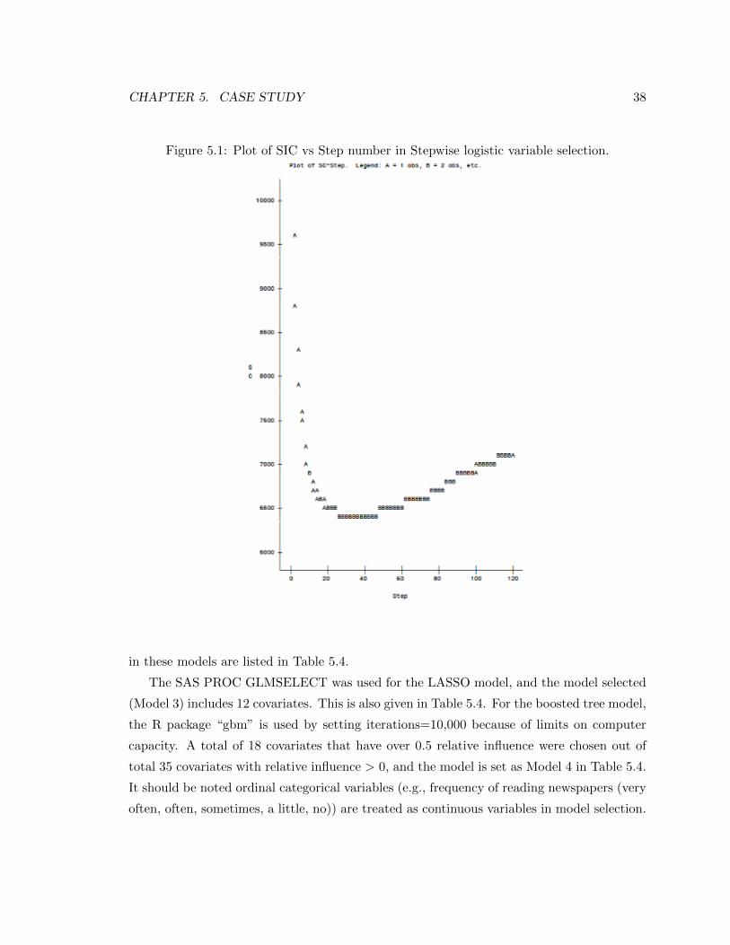
CHAPTER 5. CASE STUDY 38
Figure 5.1: Plot of SIC vs Step number in Stepwise logistic variable selection.
in these models are listed in Table 5.4.
The SAS PROC GLMSELECT was used for the LASSO model, and the model selected
(Model 3) includes 12 covariates. This is also given in Table 5.4. For the boosted tree model,
the R package “gbm” is used by setting iterations=10,000 because of limits on computer
capacity. A total of 18 covariates that have over 0.5 relative influence were chosen out of
total 35 covariates with relative influence > 0, and the model is set as Model 4 in Table 5.4.
It should be noted ordinal categorical variables (e.g., frequency of reading newspapers (very
often, often, sometimes, a little, no)) are treated as continuous variables in model selection.

CHAPTER 5. CASE STUDY 39
Table 5.4: Covariates in the models
Covariate M1 M2 M3 M4 Type1 Description
region1 x x x x 16 cat major city or provincenews x x x x 5(cont) how often read newspaperi news x x x x 5(cont) how often read Internet newspaperfreetime x x x x 14 cat how to spend free time during weekendleisure x x x x 14 cat type of leisure activities wanted to domonnet x x x x 2 cat social network in case of need of moneyordcommu x x x x 8 cat participation in community activitiesstecosp x x x x 2 cat status of economic activity of spouseipspare x x x 5(cont) importance for quality of life (sparetime)rel hohead x x x 10 cat relationship to household headage5 x x 5 cat agemarital x x 4 cat marital statusfreewhom x x 5 cat with whom spend free time during weekendsatover x x 5(cont) overall level of satisfactionfutuvol x x 3 cat voluntary service in the futureworkingh x x cont working hoursstemp x x 4 cat employment statustmanner x x 5(cont) effect of traditional culture on a life (manner)safety x x 5(cont) safety of societybook x 2 cat reading booksmagz x cont book(magazine)satcivils x 5(cont) levels of satisfaction with civil servicehchildvol x x cont voluntary service time (children,senior)heduvol x cont voluntary service time (education)movie x cont movieb life x cont book (life)b other x cont book (others)perfo x cont performancedancing x cont dancingmuseum x cont museumodonate x cont donation (others)
1 # cat = number of categories for nominal variables; cont = continuous numerical variable.

CHAPTER 5. CASE STUDY 40
5.3 Distributions of covariates in web survey and reference
survey before weighting adjustment
Before applying weighting procedures to the survey data, some covariates are explored in
order to investigate the difference between web survey respondents and reference survey
respondents. Figure 5.2 shows distributions of four covariates in the models in web survey
(WEB) and reference survey (REF). WEB respondents tend to read both actual and In-
ternet newspapers more often REF respondents. The difference is larger for the Internet
newspapers. REF people tend to consider ‘spare time’ more important than WEB people.
The proportion of WEB people who consider it important (very + fairly) is 12%, while that
in REF is 20%. For the age group covariate, the proportion of Under 29 is 33% in WEB and
22% in REF, while the proportion of Over 60 is 8% in WEB and 21% in REF. As discussed
in Subsection 5.1.2, young people still tend to participate in web surveys with high relative
frequency even though age was considered in choosing the pool of volunteer panelists. The
Education level covariate (Figure 5.3) is explored even though it is not included in any of
the four models because past work has shown a relationship with participating in the web
survey. The proportion of people with postsecondary education (undergraduate + gradu-
ate) is 61% in WEB and 36% in REF, while that of ‘under middle school’ is 11% and 28%
respectively. We can say that people with higher levels of education participated more often
in the web survey, as we expect.
From the above results, we can see that there are considerable differences in many
covariates between web survey respondents and reference survey respondents.
5.4 Weighting procedures
5.4.1 Propensity score adjustment
Once models were selected, the propensity scores were estimated by equation (4.1) for the
test data set which consisted of 18,519 observations from the reference sample and 1,432 from
the web sample. Figure 5.4 shows the distribution of propensity scores based on Model 1. As
expected estimated probabilities of being in the web survey are generally low for reference
survey respondents. However, web survey respondents are more poorly classified because

CHAPTER 5. CASE STUDY 41
Figure 5.2: Distribution of 4 covariates in the models

CHAPTER 5. CASE STUDY 42
Figure 5.3: Distribution of education level
under middle high school undergraduate graduate
Education level
Rat
e
0.0
0.1
0.2
0.3
0.4
0.5 WEB
REF
Figure 5.4: Distribution of propensity scores in Model 1
WEB
Propensity score
Fre
quen
cy
0.0 0.4 0.8
050
100
150
200
REF
Propensity score
Fre
quen
cy
0.0 0.4 0.8
050
0010
000
1500
0

CHAPTER 5. CASE STUDY 43
their proportion of the combined sample is small.
After calculating propensity scores, the PSA weights were calculated in each model by
both inverse of propensity scores as weights and subclassification (using five subclasses)
as discussed in Subsection 4.2.5. As base weights (or sampling weights), post-stratification
weights4 and rim weights5 were used in the reference survey and the web survey respectively.
The quantiles of PSA weights of all models are shown in the Table 5.5. Figure 5.5 and Figure
5.6 show the distribution of the PSA weights in Model 1. Here, the weights are scaled to
match the sample size of web survey. In other words, the sum of the weights equals the
total sample size of web survey in the test data set.
For all models, the distributions of inverse propensity score weights are severely right-
skewed. For example, in Model 1, some subjects dominate the weights (minimum weight
=0.0044, first quartile=0.0112, median=0.0203, third quartile=0.0512, and maximum=
757.2). The distribution of subclassification weights shows right-skewness, but it is less se-
vere than the previous one (minimum weight=0.1081, first quartile=0.154, median=0.1965,
third quartile=0.244, and maximum=168.5). In the inverse propensity score weights, if
the probability of ‘web people’ is very small, the weight will be very large. Therefore, the
weights may be affected substantially by propensity score models or properties of the data.
In the subclassification, the effects can be reduced because the propensity scores are divided
into groups so some smoothing of extremes occurs. In addition, Model 3 and Model 4 show
slightly less skewed distributions than Model 1 and 2. Very large weights can be corrected
by fixing a maximum value as in Huh and Cho (2009). This was not attempted in this
paper.
4The post-stratification weights are calculated based on four demographic variables which include majorcity & province, urban & rural, gender, and age. They were obtained by Statistics Korea.
5The rim weights were used for sampling from the pool of all volunteers. Those were obtained by Huhand Cho.

CHAPTER 5. CASE STUDY 44
Table 5.5: Summary of PSA weights
PSA1 Min. 1st Qu. Median Mean 3rd Qu. Max.
Model 1 Inv. 0.00 0.01 0.02 1.00 0.05 757.20Sub. 0.11 0.15 0.20 1.00 0.24 168.50
Model 2 Inv. 0.00 0.01 0.01 1.00 0.03 798.60Sub. 0.11 0.16 0.20 1.00 0.26 195.10
Model 3 Inv. 0.02 0.07 0.12 1.00 0.32 678.50Sub. 0.12 0.18 0.23 1.00 0.41 231.50
Model 4 Inv. 0.02 0.07 0.15 1.00 0.35 681.40Sub. 0.12 0.17 0.22 1.00 0.40 205.80
1 Inv. = inverse propensity scores as weights; Sub.=subclassification.
Figure 5.5: Distribution of PSA weights based on inverse propensity score weights in Model1

CHAPTER 5. CASE STUDY 45
Figure 5.6: Distribution of PSA weights based on subclassification in Model 1
5.4.2 Calibration adjustment
Even though rim weights were already used for sampling in the web survey, propensity score
adjustment might affect the distribution of demographic variables. Therefore, after calculat-
ing propensity score weights, rim weighting was applied again as a calibration adjustment as
discussed in Section 4.3. The rim weights were calculated based on marginal distributions
of four demographic variables: major city & province, urban vs. rural, gender, and age
for the test data set. Table 5.6 shows the quantiles of final weights of all models after rim
weighting, and Figure 5.7 and 5.8 shows the distribution of the final weights based on Model
1. Overall, the final weights are less positive skewed than propensity score weights, and the
maximum values are smaller as well. Subclassification shows less skewed distributions than
inverse weighting.

CHAPTER 5. CASE STUDY 46
Table 5.6: Summary of final weights
PSA Min. 1st Qu. Median Mean 3rd Qu. Max.
Model 1 Inv. 0.00 0.14 0.28 1.00 0.59 172.40Sub. 0.06 0.22 0.33 1.00 0.59 66.38
Model 2 Inv. 0.00 0.13 0.27 1.00 0.63 194.50Sub. 0.08 0.25 0.35 1.00 0.56 64.45
Model 3 Inv. 0.02 0.17 0.29 1.00 0.73 60.08Sub. 0.06 0.23 0.40 1.00 0.60 45.94
Model 4 Inv. 0.01 0.16 0.30 1.00 0.69 67.09Sub. 0.06 0.21 0.30 1.00 0.58 59.96
Figure 5.7: Distribution of final weights based on inverse propensity scores as weights inModel 1

CHAPTER 5. CASE STUDY 47
Figure 5.8: Distribution of final weights based on subclassification in Model 1
5.5 Assessment methods
As described above, four models for computing propensity scores were created and two
methods for performing PSA were used. Finally, two calibration approaches—rim weighting
or none—were applied to each combination of models and PSA methods. Thus, there are
16 different bias adjustment methods being compared.
First, in order to assess whether each stratum in the subclassification method consists
of homogeneous groups, the balance of the propensity scores is checked. It is clear that
good balancing for all variables is desirable. At least, we expect that the covariates in the
models show balance. Fortunately or unfortunately, there are a lot of overlapping variables
(size = 123) between the web survey and the reference survey in this study. It is hard to
investigate all variables. Therefore, eight covariates which are included in all four models
are explored in detail to investigate the effects on balancing due to the four models. The
eight covariates are denoted as c1: major city or province (‘region1’), c2: how often read
newspaper (‘news’), c3: how often read Internet newspaper (‘i news’), c4: how to spend
free time during weekend (‘freetime’), c5: type of leisure activities wanted to do (‘leisure’),
c6: social network in case of need of money (‘monnet’), c7: participation in community

CHAPTER 5. CASE STUDY 48
activities (‘ordcommu’), c8: status of economic activity of spouse (‘stecosp’).
Furthermore, 12 variables, which are not included in the models, were chosen in order
to check balance of responses (variables of interest). Those variables were chosen by three
per each field from four fields of questions: culture & leisure, income & consumption, social
participation, and quality of life. The 12 variables are denoted as y1: time of watching TV
during weekday (‘tv wday’), y2: experience of traveling overseas (‘otour’), y3: satisfaction
with leisure activities (‘satleisure’), y4: satisfaction with income (‘satincome’), y5: expecta-
tion of future income (‘expincome’), y6: satisfaction with consumption (‘satins’), y7: social
network in case of sick (‘sicknet’), y8: social network in case of depression (‘depnet’), y9:
experience of donation (‘donate’), y10: general health self-assessment (‘health’), y11: degree
of stress (‘stress’), y12: how busy in daily life (‘busy’).
However, good balancing does not guarantee bias reduction in the response because
survey weights and further adjustment are not considered yet. Thus, the main focus is on
the performance of each procedure in terms of bias reduction. To assess this, we assume
that estimates of reference survey are “true”. Each of the 16 procedures will be assessed
based on the 12 response variables above in terms of the percentage of bias reduction, as
calculated as
p.bias(θW.A) =
[|bias(θW.U )| − |bias(θW.A)|
|bias(θW.U )|
]× 100,
where θW.U is the unadjusted estimate and θW.A is an adjusted estimate in the web survey.
5.6 Results of comparison
5.6.1 Balance check in subclassification method before applying sample
weights and further adjustment
Balance checks were conducted by statistical tests (t-test for non-categorical covariates
and χ2 test for categorical covariates) in each subclassification stratum in order to decide
whether differences between groups are significant. The tests were applied to data both
before and after subclassification propensity adjustment. For those all 8 covariates, the web
survey respondents and the reference survey respondents are significantly different before
subclassification (p-values < 0.001). Figure 5.9 shows the p-values of each covariate in
each stratum after adjustment. After adjustment, only one covariate (c1) based on Model

CHAPTER 5. CASE STUDY 49
4 showed good balance at the significance level 0.05. In the first stratum, all covariates
are balanced across models except c3 in Model 3 and c5 in Model 4. As order of stratum
increases, more covariates show significant values. However, until 4th stratum, the imbalance
is not so severe. Overall, there seems to be reasonable balance from first to fourth stratum.
In stratum 5, all except one covariate in one model are unbalanced. That may be because
most of the web respondents are gathered in the stratum 5 for all models. To illustrate,
in Model 1, the sizes of web respondents in stratum 1 to 5 are 2, 4, 25, 163 and 1234
respectively. And, in Model 3, the sizes of web respondents in each stratum are 18, 45, 116,
203 and 1106. Web respondents (sample size=1,432) are a relatively small fraction of the
REF respondents (sample size=18,519), i.e., the ratio is about 13 times. REF respondents
dominate all of the strata. Because strata are constructed by equal numbers from the
combined sample and web respondents generally do not have very low propensity socrese,
it can be expected that large numbers of web respondents are grouped in the final stratum.
For c7 covariate, in the first stratum, the χ2 test of the covariate was not applicable due
to small size. The differences among models seems much smaller than differences between
strata.
Figure 5.10 shows the balance check results for response variables treated as covariates
not in the model. This figure shows a similar trend to Figure 5.9. Model 3 appears to
be more unbalanced in stratum 2 and stratum 4 for a few variables. However, overall, all
models seem to be balanced until stratum 4. In stratum 5, unlike the covariates in Figure
5.9, four responses are balanced. The balance seems to be reasonable except final stratum.
5.6.2 Bias reduction
For each variable of interest, there is a REF estimate (assumed to be the population value),
one unadjusted WEB estimate, and 16 estimates from the web sample based on different
combinations of adjustment: (Propensity Score Model 1, 2, 3 and 4) × (Inverse weighting
and Subclassification) × (No Calibration and Rim weighting). For variables which were
measured on a Likert scale6, mean scale values are used for the estimates. Table 5.7 and
Table 5.8 show the results including percentage of bias reduction (p.bias). A large p.bias
6The Likert scale is often used to measure respondents’ attitudes by asking the extent to which they agreeor disagree with a particular question or statement. A typical scale might be “strongly agree, agree, neutral,disagree, strongly disagree” and this is often considered as ordinal data.

CHAPTER 5. CASE STUDY 50
Figure 5.9: Balance check for covariates in the models
●
●●
●
●
●
●
Balance in Stratum 1
Covariates
p−va
lues
0.0
0.4
0.8
c1 c2 c3 c4 c5 c6 c7 c8
●
●
●
●
●
●
●
●
Balance in Stratum 2
Covariates
p−va
lues
0.0
0.4
0.8
c1 c2 c3 c4 c5 c6 c7 c8
●
● ●
●
●
●
● ●
Balance in Stratum 3
Covariates
p−va
lues
0.0
0.4
0.8
c1 c2 c3 c4 c5 c6 c7 c8
●
●
●
●
●
●
●
●
Balance in Stratum 4
Covariates
p−va
lues
0.0
0.4
0.8
c1 c2 c3 c4 c5 c6 c7 c8
● ● ● ● ● ● ● ●
Balance in Stratum 5
p−va
lues
0.0
0.4
0.8
c1 c2 c3 c4 c5 c6 c7 c8
● M1M2M3M4

CHAPTER 5. CASE STUDY 51
Figure 5.10: Balance check for variables of interest
●
●●
● ●
●●
●●
●●
Balance in Stratum 1
Variables of Interest
p−va
lues
0.0
0.4
0.8
y1 y3 y5 y7 y9 y11
●
●
●
●
●●
●
●
●●
●
●
Balance in Stratum 2
Variables of Interest
p−va
lues
0.0
0.4
0.8
y1 y3 y5 y7 y9 y11
●
●
●
●
●
●
● ●
●
●
●
●
Balance in Stratum 3
Variables of Interest
p−va
lues
0.0
0.4
0.8
y1 y3 y5 y7 y9 y11
●
●
● ●
●
●
●
● ●
●
●●
Balance in Stratum 4
Variables of Interest
p−va
lues
0.0
0.4
0.8
y1 y3 y5 y7 y9 y11
●
●
● ● ● ●
●
●
● ● ●●
Balance in Stratum 5
p−va
lues
0.0
0.4
0.8
y1 y3 y5 y7 y9 y11
● M1M2M3M4

CHAPTER 5. CASE STUDY 52
means that the adjustment performed bias reduction to a greater degree because p.bias is
a measure of bias in adjusted estimates relative to unadjusted estimates. A negative p.bias
means that the bias gets worse after adjustment.
Each variable shows very different bias reduction rates according to each combination
of adjustment. Figure 5.11 shows the results visually. To decide which combination ac-
complishes bias reduction best across all variables, ANOVA analysis was conducted. Tukey
multiple comparisons of means were conducted as well. Table 5.9 shows the ANOVA table.
All of factors are significant except three-way interaction and model:psa, which is marginal
(p=0.08). For models, Model 3 (mean = -29%) and Model 4 (mean=-41%) are not sig-
nificantly different. However Model 3 may perform slightly better than Model 4. Models
3 and 4 perform better than Model 1 (mean=-133%) and Model 2 (mean=-143%). For
PSA methods, subclassification method (mean=-18%) performs better than inverse weight-
ing (mean=-156%). For calibration factor, applying the calibration (mean=-4%) performs
better than no adjustment (mean=-169%). Therefore, we can say tentatively that Model
3 with subclassification and calibration adjustment performs “best”. The average value of
percentage of bias reduction in this combination, the LASSO model with PSA and calibra-
tion adjustment, is 25%. Figure 5.12 shows the bias reduction rate of each variable in this
combination. The ratio of bias reduction out of all variables (i.e., p.bias > 0) is 67% and
the ratio of substantial bias reduction (i.e., p.bias > 50) is 42%. The worst case is observed
in y3 variable, for which bias reduction is -97%.

CHAPTER 5. CASE STUDY 53
y1
y2
y3
y4
y5
y6
est.1
p.b
ias
est.1
p.b
ias
est.1
p.b
ias
est.1
p.b
ias
est.1
p.b
ias
est.1
p.b
ias
RE
F2.8
90.
133.
132.
271.
893.
34U
nad
just
ed2.3
60.
152.
982.
221.
603.
26M
1.In
v.n
2.60
46
0.01
-790
2.32
-453
2.65
-756
2.90
-239
2.69
-689
M2.
Inv.n
2.58
42
0.01
-822
2.25
-501
2.61
-673
2.96
-257
2.65
-742
M3.
Inv.n
2.77
78
0.06
-447
3.02
262.
56-5
492.
24-1
43.
18-9
6M
4.In
v.n
2.69
63
0.08
-319
2.95
-19
2.63
-700
2.26
-21
3.18
-101
M1.
Su
b.n
2.44
15
0.09
-217
2.95
-21
2.59
-619
2.14
193.
19-8
4M
2.S
ub
.n2.
5027
0.08
-296
2.90
-56
2.60
-641
2.17
73.
19-8
7M
3.S
ub
.n2.
6758
0.09
-206
2.99
62.
2883
1.79
663.
25-9
M4.
Su
b.n
2.49
25
0.13
532.
89-6
32.
38-1
461.
8071
3.32
69M
1.I
nv.C
2.2
0-3
00.
12-1
92.
82-1
082.
33-4
41.
8585
3.20
-76
M2.I
nv.C
2.1
5-3
90.
11-7
02.
76-1
502.
3035
1.88
943.
16-1
19M
3.I
nv.C
2.4
721
0.12
362.
98-1
2.19
-70
1.56
-13
3.31
62M
4.I
nv.C
2.3
97
0.14
222.
86-8
42.
3039
1.60
33.
2820
M1.
Su
b.C
2.2
9-1
20.
1439
2.97
-62.
33-3
01.
7553
3.25
-19
M2.
Su
b.C
2.3
1-9
0.12
322.
95-1
82.
3037
1.77
593.
26-0
M3.
Su
b.C
2.4
516
0.12
182.
96-1
52.
18-9
31.
58-4
3.31
57M
4.S
ub
.C2.3
6-1
0.16
-82
2.83
-101
2.28
631.
615
3.33
89
1p
opu
lati
onva
lue,
un
adju
sted
esti
mat
eof
web
sam
ple
,an
des
tim
ates
ofw
ebsa
mp
lein
each
com
bin
atio
nof
adju
stm
ents
.
Tab
le5.
7:P
erce
nta
geof
bia
sre
du
ctio
n(p
.bia
s)in
16co
mb
inat
ion
ofad
just
men
t(1
)

CHAPTER 5. CASE STUDY 54
y7
y8
y9
y10
y11
y12
est.1
y1.
bes
t.1
y2.
bes
t.1
y3.
bes
t.1
y4.
bes
t.1
y5.
bes
t.1
y6.
b
RE
F0.
770.
820.
322.
792.
522.
61U
nad
just
ed0.
810.
850.
352.
612.
282.
50M
1.I
nv.n
0.9
8-3
760.
98-3
870.
38-1
252.
6313
3.30
-233
1.76
-699
M2.I
nv.n
0.9
9-3
940.
99-4
100.
40-2
242.
60-2
3.35
-257
1.66
-796
M3.I
nv.n
0.8
9-1
640.
91-1
820.
15-6
012.
8660
2.71
202.
36-1
37M
4.I
nv.n
0.8
9-1
740.
92-1
860.
15-5
952.
8660
2.70
252.
26-2
26M
1.S
ub
.n0.8
5-7
90.
87-5
20.
30-0
2.70
502.
7022
2.37
-130
M2.S
ub
.n0.8
5-8
90.
88-7
90.
3137
2.70
542.
6927
2.48
-25
M3.S
ub
.n0.8
3-3
20.
86-1
40.
25-2
102.
7998
2.56
842.
6088
M4.S
ub
.n0.8
4-5
70.
86-1
80.
27-1
282.
7791
2.55
862.
42-8
1M
1.In
v.C
0.81
10.
87-4
70.
39-1
692.
57-1
72.
5970
2.21
-276
M2.
Inv.C
0.80
19
0.87
-63
0.41
-251
2.53
-40
2.61
622.
19-2
92M
3.In
v.C
0.79
42
0.84
420.
27-9
72.
7686
2.45
722.
6110
0M
4.In
v.C
0.82
-10
0.84
310.
27-1
072.
7895
2.47
822.
5650
M1.S
ub
.C0.
81-7
0.85
-80.
3362
2.65
222.
5195
2.33
-160
M2.S
ub
.C0.
8018
0.85
-00.
3439
2.64
222.
4573
2.36
-135
M3.S
ub
.C0.
8025
0.83
600.
29-9
2.73
702.
4677
2.61
97M
4.S
ub
.C0.
82-2
60.
8435
0.29
-17
2.76
832.
5210
02.
5219
1p
op
ula
tion
valu
e,u
nad
just
edes
tim
ate
ofw
ebsa
mp
le,
and
esti
mat
esof
web
sam
ple
inea
chco
mb
inat
ion
of
adju
stm
ents
.
Tab
le5.8
:P
erce
nta
geof
bia
sre
du
ctio
n(p
.bia
s)in
16co
mb
inat
ion
ofad
just
men
t(2
)
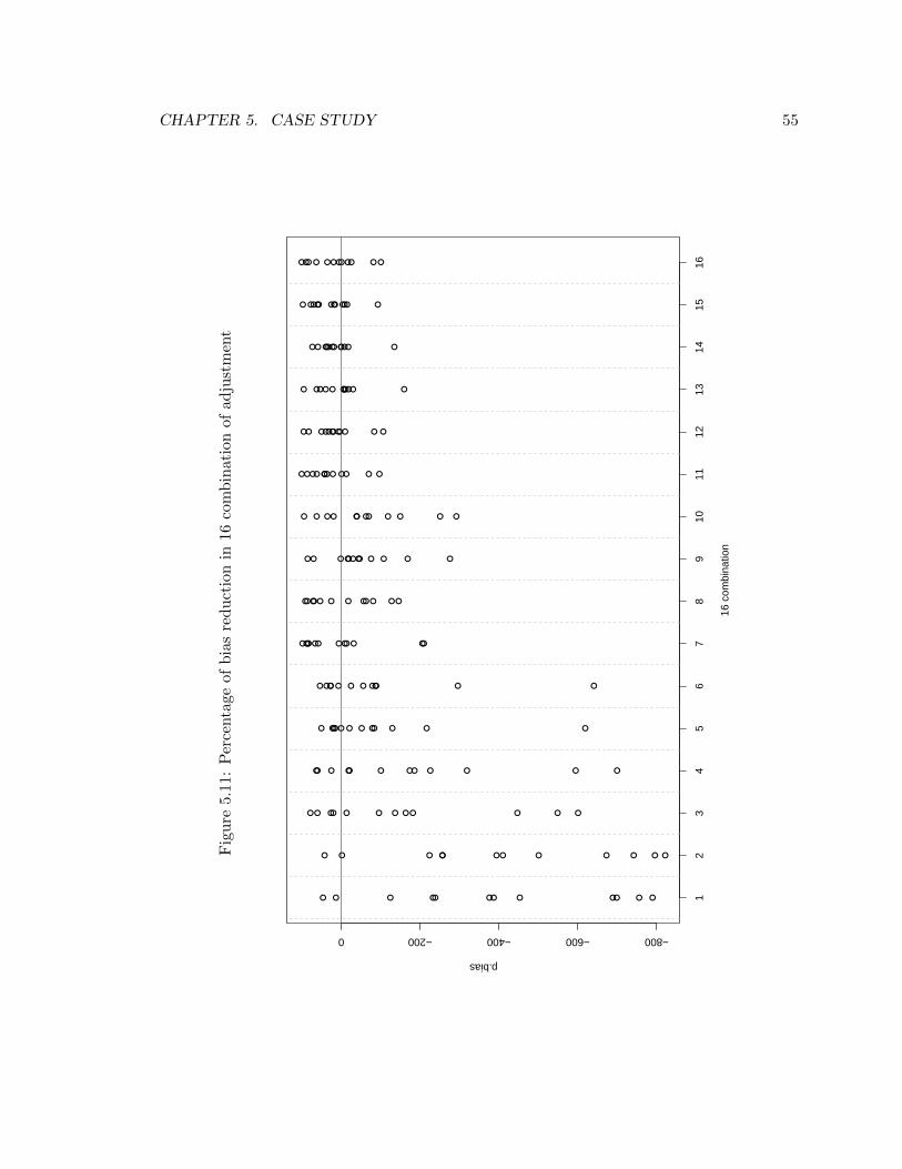
CHAPTER 5. CASE STUDY 55
Fig
ure
5.11
:P
erce
nta
geof
bia
sre
du
ctio
nin
16co
mb
inat
ion
ofad
just
men
t
● ●● ●● ●● ●●● ● ●
● ●● ●● ●● ●●● ● ●
● ●● ●● ● ● ● ●● ● ●
● ●● ●● ● ● ● ●● ● ●
● ●● ●● ●●●●● ● ●
● ●● ●● ● ●●●● ● ●
● ●●● ● ● ●● ●● ●●
●● ● ●● ● ●● ●● ● ●
●● ●●● ●● ● ●●● ●
● ● ●●● ●● ● ●●● ●
●● ● ●●● ●● ●● ●●
●● ●● ●● ●● ●● ● ●
●● ● ●● ●● ●● ●● ●
●● ●●● ●● ●● ●● ●
●● ● ●●● ●● ●●●●
● ● ●● ●● ●● ●●● ●
16 c
ombi
natio
n
p.bias
−800−600−400−2000
12
34
56
78
910
1112
1314
1516

CHAPTER 5. CASE STUDY 56
Table 5.9: ANOVA table for effects of model and adjustment
Df Sum Sq Mean Sq F value Pr(>F)1
var 11 1560639.14 141876.29 7.44 0.000 ***model 3 510577.60 170192.53 8.92 0.000 ***psa 1 914250.01 914250.01 47.92 0.000 ***cal 1 1303996.51 1303996.51 68.35 0.000 ***model:psa 3 131224.47 43741.49 2.29 0.080 .model:cal 3 156369.64 52123.21 2.73 0.046 *psa:cal 1 519896.26 519896.26 27.25 0.000 ***model:psa:cal 3 17740.31 5913.44 0.31 0.818Residuals 165 3147899.78 19078.18
1 Significance codes: 0 ‘***’ 0.001 ‘**’ 0.01 ‘*’ 0.05 ‘.’ 0.1 ‘ ’ 1
Figure 5.12: Bias reduction rate in LASSO model with subclassification and rim weightingadjustments
●●
●
●
●
●
●
●
●
●
●
●
Variables of Interest
p.bi
as
−10
0−
500
5010
0
y1 y2 y3 y4 y5 y6 y7 y8 y9 y10 y11 y12

Chapter 6
Discussion and Conclusion
This project explored the relative merits of different models, different propensity score
adjustment methods and calibration adjustment for reducing bias in volunteer panel web
survey. In Section 6.1, the evaluation of the results of this case study and some discussion
are given. Section 6.2 concludes this project.
6.1 Discussion
The best case, the LASSO model with subclassification PSA and calibration adjustment,
shows that bias reduction occurred in 67% variables out of total twelve variables. The
proportion of over 50% bias reduction rate is 42% variables. The proportions seems to be
reasonable compared to the result of Hur and Cho’s research (79% and 35%, respectively).
However, overall, a lot of negative bias reductions are observed specially in combinations
where PSA was done without calibration. This fact implies PSA adjustments did not work
well alone for my data set. It casts doubt on the PSA adjustment in this case study.
I believe that part of the immense failure of PSA using subclassification is the poor
balance achieved in Stratum 5 (Figure 5.4). Table 6.1 shows how the combined sample was
distributed in each stratum in Model 1 for the test data set. Partitioning the total sample
into 5 groups creates 3 groups consisting of propensity scores in the 0-0.02 range. The last
group covers the 0.08-1.0 range, which contains massively heterogeneous people. Assigning
them a common adjustment is a poor idea. Meanwhile, the very tiny WEB sample sizes
in the first group leads to a massive weight being applied to them. It may be corrected by
setting maximum value of weights to 5 or something. However, it is speculative because
57

CHAPTER 6. DISCUSSION AND CONCLUSION 58
Table 6.1: Average propensity scores for each survey in 5 strata in Model 1
WEB REFStratum mean range size mean range size
1 4.4e-5 [4.3e-5, 4.5e-5] (2) 6.7e-5 [3.7e-8, 2.4e-4] (3938)2 0.002 [4.9e-4, 2.6e-3] (4) 0.001 [2.4e-4, 2.8e-3] (3986)3 0.008 [0.003, 0.014] (25) 0.007 [0.003, 0.014] (3966)4 0.05 [0.016, 0.078] (163) 0.04 [0.015, 0.081] (3827)5 0.48 [0.082, 0.991] (1238) 0.23 [0.081, 0.955] (2752)
(#) is the sample size for each survey in each stratum
there is no guideline for the maximum value for all surveys. Even if a certain maximum
value worked well for my data set, it would not guarantee that the value works for other
survey data.
It would appear that a different subclassification algorithm needs to be employed. This
would be a whole new piece of research, but perhaps someone at Statistics Korea will want
to take it on. For example, it might be possible to find a formula for the variance of
weights that depends on both the number of cases from each group within a stratum and
the variability of propensity scores with the stratum.
Another possible solution to improvement of bias reduction may be a matching method.
For my data, the proportion of sample size of the web survey vs. that of the reference
survey is relatively small. Even though the web sample size (2,903) is large enough, the
small proportion caused imbalance in subclassification method and eventually caused the
creation of huge weights. A matching method can be performed well where there are a
limited number of treated group members and a larger number of control group members.
In order to use a matching method, it is necessary to select the web sample from reference
survey respondents because the matching estimator for mean of a response works only
when common sample weights are available. That means we should invite reference survey
respondents to participate in web surveys. It seems to be worthwhile to try in future surveys.
Another reason for the poor result may be violation of some assumptions made during
the analysis. The most important assumption in PSA adjustment is the ‘strong ignorability
assumption’ which means responses in the web survey have a similar distribution to those in
the reference survey given covariates. This assumption might be violated, resulting in poor
CHAPTER 6. DISCUSSION AND CONCLUSION 59
bias correction. Another assumption like MAR is hard to detect. It is also hard to detect
whether mode effects between web survey and face-to-face survey can be discardable.
An interesting thing is that all three variables (y10, y11, and y12), which were chosen
from ‘quality of life’ field of questions, show over 70% bias reduction rate in the “best”
combination (Figure 5.12). This fact might imply that adjustment method applied in this
study worked well for a certain field of questions.
Variable selection in the propensity score model is also a critical issue. In this study,
LASSO and boosted tree models perform better than stepwise models. According to the
covariates in the models, the results became significantly different. It is notable that many
covariates in the model does not guarantee good performance, at least for the data used in
this study. It is important to choose appropriate webographic variables. Expert knowledge,
not a statistical approach, may be helpful in variable selection (Flom and Cassell, 2008). It
is necessary to study webographic variables further.
Variance was not dealt with in this study, but it should be studied in future research
in order to evaluate adjustment methods. While bias reduction is desirable, it does not
mean a reduction of mean square error (MSE). In general, weighting adjustment increases
variance. It may increase the MSE. According to Schonlau et al. (2007), bias dominates the
MSE after adjustment in many cases. However, an increase of variance sometimes leads to
an overall increase of the MSE.
6.2 Conclusion
Web surveys have become popular recently because of their attractive advantages in data
collection discussed in Chapter 1. However, web surveys based on non-probability sampling
cause problems such as selection errors, coverage errors and non-response errors. Many
researchers have studied web surveys, especially volunteer web panel surveys, in order to
correct the bias due to the above problems. So far, they have applied propensity score adjust-
ment and calibration adjustment for web surveys. For PSA adjustment, inverse propensity
scores and subclassification weighting methods were explored. For calibration adjustment,
rim weighting was used for this case study.
Lee and Valliant (2009) show that these adjustments work well for the simulated data.
However, study results of many other researchers do not seem to be so good. It may be
because that, in the real world, assumptions made in applying adjustments are violated.

CHAPTER 6. DISCUSSION AND CONCLUSION 60
In particular, PSA adjustment may not work for large surveys because it is hard to meet
‘strong ignorability assumption’ for all responses.
Nonetheless, I definitely believe that researches of web surveys should keep going on
because the advantages of web surveys are substantial. In terms of national statistical
agencies, they suffer from getting information from people because of a growing concern for
privacy. It is obvious that the problem will get worse in the future. A volunteer panel web
survey may be a good alternative so long as the analysis is proper.

Appendix A
Description of covariates
All overlapping covariates are described here. The #cat means number of categories for
nominal variables and cont means continuous numerical variable in type. The ordinal cate-
gorical variables are treated as continuous variables in model selection. The ‘-’ in description
field means sub question of above no ‘-’ question.
61

APPENDIX A. DESCRIPTION OF COVARIATES 62
Figure A.1: Description of all covariates (1)
Covariate Type Description Coding
region1 16 cat major city or province
1=Seoul, 2=Busan, 3= Daegu, 4= Incheon, 5= Kwangju, 6= Deajeon, 7= Ulsan , 8= Kyeonki, 9= Kangwon, 10= Chungbuk, 11= Chungnam 12= Chenbuk 13=Chennam, 14= kyengbuk, 15= Kyeonnam, 16=Jeju
region2 2 cat urban or rural 1=urban, 2=rural
gender 2 cat gender 1=male, 2=female
age5 5 cat age group 1= under 29, 2=30-‐39, 3=40-‐49, 4=50-‐59, 5=over 60
educ4 4 cat education level 1=under middle, 2=high, 3=undergraduate, 4=graduate
ty_living 5 cat type of living quarter 1=house, 2=APT, 3=townhouse, 4=multiplex, 5=others
ty_occup 5 cat type of occupancy
1=landlord, 2=big lump sum at the beginning without monthly rent fee 3=monthly rent with variable deposit, 4=monthly Rent without variable Deposit, 5=free
rel_hohead 10 cat relationship to household head
1=head, 2=spouse, 3=single son/daughter, 4=married son/daughter, 5=grandchildren, 6=parent, 7=grandparent, 8=single sibling, 9=other relatives, 10=others
marital 4 cat marital status 1=single, 2=married, 3=bereaved 4=divorced
news 5(cont) how often read newspaper
1=nearly everyday, 2=three or four times a week, 3=one or two times a week, 4=one time every second week, 5=no
i_news 5(cont) how often read internet newspaper
1=nearly everyday, 2=three or four times a week, 3=one or two times a week, 4=one time every second week, 5=no
tv 2 cat watching TV 1=yes, 2=no
tv_wday cont -‐ time during weekday time in hours for one day
tv_sa cont -‐ time during Saturday time in hours
tv_su cont -‐ time during Sunday/Holiday time in hours

APPENDIX A. DESCRIPTION OF COVARIATES 63
Figure A.2: Description of all covariates (2)
Covariate Type Description Coding
book 2 cat reading books 1=yes, 2=no
magz cont -‐ magazine number of volumes
b_educ cont -‐ educational book number of volumes
b_job cont -‐ job number of volumes
b_life cont -‐ life number of volumes
b_other cont -‐ others number of volumes
dtour 2 cat domestic tour 1=yes, 2=no
d_night cont -‐ number of night tour number of night tour
d_m_night cont -‐ mean of nights per each tour mean of nights per each tour
d_day cont -‐ number of day trip number of day trip
otour 2 cat experience of traveling overseas for 1 year 1=yes, 2=no
o_sight cont -‐ number of sightseeing number of sightseeing
o_family cont -‐ number of family visiting number of family visiting
o_busi cont -‐ number of business number of business
o_lang cont -‐ number of language study number of language study
o_life 2 cat -‐ in case no, experience of traveling overseas for whole life
1=yes, 2=no
recre 2 cat use of recreational facilities 1=yes, 2=no
attract cont -‐ # of tourist attraction number of visiting
spa cont -‐ # of spa number of visiting
beach cont -‐ # of beach number of visiting
mount cont -‐ # of mountain number of visiting

APPENDIX A. DESCRIPTION OF COVARIATES 64
Figure A.3: Description of all covariates (3)
Covariate Type Description Coding
park cont -‐ # of amusement park number of visiting
cultevent 2 cat visiting cultural facilities and sporting events or verves
1=yes, 2=no
concert cont -‐ # of concert number of visiting
perfo cont -‐ # of performance number of visiting
dancing cont -‐ # of dancing number of visiting
movie cont -‐ # of movie number of visiting
museum cont -‐ # of museum number of visiting
gallary cont -‐ # of art gallery number of visiting
sports cont -‐ # of sports number of visiting
freetime 14 cat how to spend free time during weekend (1st)
1=TV or Video, 2=tour, 3=cultural facilities, 4=watching sporting event, 5=spots activity, 6=computer game or internet, 7=creational hobby, 8=learning, 9=volunteer activity, 10=religion activity, 11=housework, 12=rest, 13=social activity, 14=others
freewhom 5 cat with whom spend free time during weekend 1=family, 2=friend, 3=club, 4=alone, 5=others
leisure 14 cat type of leisure activities wanted to do(1st)
1=TV or Video, 2=tour, 3=cultural facilities, 4=watching sporting event, 5=spots activity, 6=computer game or internet, 7=creational hobby, 8=learning, 9=volunteer activity, 10=religion activity, 11=housework, 12=rest, 13=social activity, 14=others
satleisure 5(cont) satisfaction with leisure activities 1=very satisfied, ... 5=very dissatisfied
leisuredis 9 cat reasons for dissatisfaction with leisure activities
1=economic, 2=shortage of time, 3=inconvenience of transportation, 4=shortage of leisure facilities, 5=shortage of information or program, 6=no hobby, 7=health, 8=no persons to do together, 9=others

APPENDIX A. DESCRIPTION OF COVARIATES 65
Figure A.4: Description of all covariates (4)
Covariate Type Description Coding
effect of traditional culture on life
tcere 5(cont)
-‐ the four ceremonial occasions of coming of age, wedding, funeral, and ancestral rites
1=very affected, -‐-‐-‐, 5=very unaffected
tmanner 5(cont) -‐ manners 1=very affected, -‐-‐-‐, 5=very unaffected
fgame 5(cont) -‐ folk game 1=very affected, -‐-‐-‐, 5=very unaffected
tarts 5(cont) -‐ traditional arts 1=very affected, -‐-‐-‐, 5=very unaffected
tfood 5(cont) -‐ traditional food 1=very affected, -‐-‐-‐, 5=very unaffected
tcloth 5(cont) -‐ traditional cloth 1=very affected, -‐-‐-‐, 5=very unaffected
thouse 5(cont) -‐ traditional house 1=very affected, -‐-‐-‐, 5=very unaffected
tmarital 5(cont) -‐ traditional martial arts 1=very affected, -‐-‐-‐, 5=very unaffected
income 2 cat having income 1=yes, 2=no
satincome 5(cont) -‐ Level of satisfaction with income 1=very satisfied, -‐-‐-‐, 5=very dissatisfied
expincome 5(cont) -‐ expectation of future income 1=very increase-‐-‐-‐5=very decrease
incomedist 5(cont) opinion on income distribution 1=very fair,-‐-‐-‐, 5=very unfair
satcons 5(cont) satisfaction with a daily life as a consumer 1=very satisfied, -‐-‐-‐, 5=very dissatisfied
satover 5(cont) overall level of satisfaction 1=very satisfied, -‐-‐-‐, 5=very dissatisfied
sicknet 2 cat social network in case of sick 1=yes, 2=no
nsicknet Cont -‐ # of people to help number of people to help
monnet 2 cat social network in case of need of money 1=yes, 2=no
nmonnet Cont -‐ # of people to help number of people to help

APPENDIX A. DESCRIPTION OF COVARIATES 66
Figure A.5: Description of all covariates (5)
Covariate Type Description Coding
deprnet 2 cat social network in case of depression 1=yes, 2=no
ndepnet Cont -‐ # of people to help number of people to help
donate 2 cat donations 1=yes, 2=no
ddonate Cont -‐ direct number of donations
pdonate Cont -‐ press number of donations
sdodate Cont -‐ social service number of donations
rdonate Cont -‐ religious group number of donations
wdonate Cont -‐ workplace number of donations
odonate Cont -‐ others number of donations
commu 2 cat participation in community activities 1=yes, 2=no
ordcommu 8 cat -‐ 1st order 1=friendly, 2=religion, 3=hobby & sports & leisure, 4=volunteer, 5=academic, 6=interest, 7=political, 8=others
volunt 2 cat voluntary service 1=yes, 2=no
envvol Cont -‐ envirionment, crime prevention (#) number of participations
henvvol Cont -‐ envirionment, crime prevention(time) hours during each participation
govvol Cont -‐ government event(#) number of participations
hgovvol Cont -‐ government event(time) hours during each participation
eduvol Cont -‐ education(#) number of participations
heduvol Cont -‐ education(time) hours during each participation
childvol Cont -‐ children,senior(#) number of participations
hchildvol Cont -‐ children,senior(time) hours during each participation
disvol Cont -‐ disaster(#) number of participations

APPENDIX A. DESCRIPTION OF COVARIATES 67
Figure A.6: Description of all covariates (6)
Covariate Type Description Coding
hdisvol Cont -‐ disaster(time) hours during each participation
othvol Cont -‐ others(#) number of participations
hothvol Cont -‐ others(time) hours during each participation
futuvol 3 cat voluntary service in the future 1=yes, 2=yes, but not now, 3=no
civils 2 cat having civil service 1=yes, 2=no
satcivils 5(cont) -‐ levels of satisfaction with civil service 1=very satisfied, -‐-‐-‐, 5=very dissatisfied
discivils 8 cat -‐ reasons for dissatisfaction with civil service(1st)
1=unkind, 2=long time, 3=difficult procedures, 4=unfair, 5=unskilled, 6=shortage of amenities, 7=bribe, 8=others
classaw 6 cat class awareness 11=high-‐high, 12-‐high-‐low, 21=middle-‐high, 22=middle-‐low, 31=low-‐high, 32=low-‐low
clswg 5(cont) class mobility within generation
1=very high, 2=somewhat high, 3=somewhat low, 4=very low, 5=don't know
clsng 5(cont) class mobility future generation
1=very high, 2=somewhat high, 3=somewhat low, 4=very low, 5=don't know
health 5(cont) general health 1=very good,-‐-‐-‐,5=very bad
stress 4(cont) stress 1=very high, 2=high, 3=somewhat, 4=almost not
satres 5(cont) Satisfacion with residential district 1=very satisfied, -‐-‐-‐, 5=very dissatisfied
safety 5(cont) safety of society 1=very safe,-‐-‐-‐, 5=very unsafe
crime 5(cont) fear of crime 1=very much,-‐-‐-‐, 5=very little
satfam 5(cont) satisfaction with family 1=very satisfied, -‐-‐-‐, 5=very dissatisfied
contam 5(cont) feeling of degree of contamination 1=very improved,-‐-‐-‐, 5=very worsen
suicide 2 cat suicidal thinking 1=yes, 2=no
busy 5(cont) life time -‐ busy 1=always busy,-‐-‐-‐, 5=not at all

APPENDIX A. DESCRIPTION OF COVARIATES 68
Figure A.7: Description of all covariates (7)
Covariate Type Description Coding
importance for quality of life
ipincom cont -‐ income/consumption from 1 to 5 according to importance
iphealth cont -‐ health from 1 to 5 according to importance
iplabor cont -‐ labour from 1 to 5 according to importance
ipeduc cont -‐ education from 1 to 5 according to importance
ipresi cont -‐ residence/transportation from 1 to 5 according to importance
ipsaftey cont -‐ safety from 1 to 5 according to importance
ipfam cont -‐ family from 1 to 5 according to importance
ipenv cont -‐ environement from 1 to 5 according to importance
ipinteg cont -‐ social integration from 1 to 5 according to importance
ipspare cont -‐ sparetime from 1 to 5 according to importance
stecono 2 cat status of economic activity 1=yes, 2=no
workingh cont -‐ working hours hours for a week
stemp 4 cat -‐ employment status 1=employee, 2=employer, 3=self-‐employment, 4=work without pay
stecosp 2 cat status of economic activity of spouse 1=yes, 2=no
famincom 9(cont) family income for a month
1=under 500$, 2='500$~1000$', 3='1000$~2000$', 4='2000$~3000$, 5='3000$~4000$', 6='4000$~5000$', 7='5000$~6000$', 8='6000$~7000$', 9=over 7000$

Bibliography
Andridge, R. R. and Little, R. J. A. (2010). A review of hot deck imputation for surveynon-response. International Statistical Review , 78(1), 40–64.
Bandilla, W., Bosnjak, M., and Altdorfer, P. (2003). Survey administration effects? SocialScience Computer Review , 21(2), 235–243.
Berson, I. R., Berson, M. J., and Ferron, J. M. (2002). Emerging risks of violence in thedigital age: Lessons for educators from an online study of adolescent girls in the unitedstates. Journal of School Violence, 1(2), 51–71.
Bethlehem, J. (2010). Selection bias in web surveys. International Statistical Review , 78(2),161–188.
Brookhart, M. A., Schneeweiss, S., Rothman, K. J., Glynn, R. J., Avorn, J., and Strmer,T. (15 June 2006). Variable selection for propensity score models. American Journal ofEpidemiology , 163(12), 1149–1156.
Cervantes, I. F., Brick, M. J., and Jones, M. (2009). Efficacy of post-stratification in complexsampling designs. In JSM 2009 .
Cochran, W. G. (1968). The effectiveness of adjustment by subclassification in removingbias in observational studies. Biometrics, 24(2), pp. 295–313.
Couper, M. P. (2000). Review: Web surveys: A review of issues and approaches. PublicOpinion Quarterly , 64(4), 464–494.
Couper, M. P. (2005). Technology trends in survey data collection. Social Science ComputerReview , 23(4), 486–501.
D’Agostino, R. B. D. (1998). Tutorial in biostatistics propensity score methods for biasreduction in the comparison of a treatment to a non-randomized control group. Statisticsin Medicine, 2281(19), 2265–2281.
Deming, W. E. and Stephan, F. F. (1940). On a least squares adjustment of a sampled fre-quency table when the expected marginal totals are known. The Annals of MathematicalStatistics, 11(4), pp. 427–444.
69

BIBLIOGRAPHY 70
Deville, J.-C. and Sarndal, C.-E. (1992). Calibration estimators in survey sampling. Journalof the American Statistical Association, 87(418), pp. 376–382.
Duffy, C., Smith, K., Terhanian, G., and Bremer, J. (2005). Comparing data from onlineand face-to-face surveys. Social Science Computer Review .
Elith, J., Leathwick, J. R., and Hastie, T. (2008). A working guide to boosted regressiontrees. Journal of Animal Ecology , 77, 802–813.
Flom, P. L. and Cassell, D. L. (2008). Stopping stepwise: Why stepwise and similar selectionmethods are bad, and what you should use. In PNWSUG 2008 .
Fricker, R. D. J. (2008). Sampling Methods for Web and E-mail Surveys, pages 195–216.SAGE Publications, Ltd.
Hahs-Vaughn, D. and Onwuegbuzie, A. J. (2006). Estimating and using propensity scoreanalysis with complex samples. The Journal of Experimental Education, 75(1), 31–65.
Horvitz, D. G. and Thompson, D. J. (1952). A generalization of sampling without replace-ment from a finite universe. Journal of the American Statistical Association, 47(260),pp. 663–685.
Huh, M. H. and Cho, S. K. (2009). Propensity adjustment weighting of the internet surveyby volunteer panel. Report for Statistics Korea.
Lee, S. (2004). Statistical estimation methods in volunteer panel web surveys. Ph.D. thesis,University of Maryland.
Lee, S. and Valliant, R. (2009). Estimation for volunteer panel web surveys using propensityscore adjustment and calibration adjustment. Sociological Methods & Research, 37(3),319–343.
Little, R. J. A. and Wu, M.-M. (1991). Models for contingency tables with known mar-gins when target and sampled populations differ. Journal of the American StatisticalAssociation, 86(413), pp. 87–95.
Loosveldt, G. and Sonck, N. (2008). An evaluation of the weighting procedures for anonline access panel survey. Survey Research Methods, 2(2). Retrieved July 14, 2011,from http://w4.ub.uni-konstanz.de/srm/article/view/82/1657.
Lozar, M. K., Bosnjak, M., Berzelak, J., Haas, I., and Vehovar, V. (2008). Web surveys ver-sus other survey modes: A meta-analysis comparing response rates. nternational Journalof Market Research, 50(1), 79–104.
Malhotra, N. and Krosnick, J. A. (2007). The effect of survey mode and sampling oninferences about political attitudes and behavior: Comparing the 2000 and 2004 anes tointernet surveys with nonprobability samples. Political Analysis, 15(3), 286–323.

BIBLIOGRAPHY 71
Panacek, E. A. and Thompson, C. B. (2007). Sampling methods: Selecting your subjects.Air Medical Journal , 26(2), 75 – 78.
Roe, B. P., Yang, H.-J., and Zhu, J. (2005). Boosted decision trees, a powerful eventclassifier. In Statistical problems in particle physics, astrophysics and cosmology , pages139–142.
Rosenbaum, P. R. and Rubin, D. B. (1983). The central role of the propensity score inobservational studies for causal effects. Biometrika, 70(1), 41–55.
Rosenbaum, P. R. and Rubin, D. B. (1984). Reducing bias in observational studies usingsubclassification on the propensity score. Journal of the American Statistical Association,79(387), pp. 516–524.
Roth, V. (2004). The generalized lasso. Neural Networks, IEEE Transactions on, 15(1), 16–28.
Schonlau, M., van Soest, A., and Kapteyn, A. (2007). Beyond demographics: Are ‘webo-graphic’ questions useful for reducing the selection bias in web surveys? In JSM 2007 .
Shtatland, E. S., Kleinman, K., and Cain, E. M. (2008). Stepwise methods in using sas R©proc logistic and sas R© enterpise minertm for prediction. SAS Institute.
Steinmetz, S., Tijdens, K., and de Pedraza, P. (2009). Comparing data from online andface-to-face surveys. ESRA 2009 .
Vehovar, V., Manfreda, K., and Batagelj, Z. (1999). Web surveys: Can the weighting solvethe problem? In American Statistical Association, 1999 , pages 962–967.