statistical methods (regression)

STATISTICAL METHODS

(REGRESSION)

CSE 634 - Data Mining Concepts and Techniques

Professor Anita Wasilewska

Contents

●  Linear Regression

●  Logistic Regression ●  Bias and Variance in Regression ●  Model Fit ●  Methods to prevent Overfitting ●  Regularization Methods (Lasso and Ridge

regression) ●  Research Paper

References

●  http://www3.cs.stonybrook.edu/~cse634/L2ch2preprocess.pdf - Lecture Slides ●  http://www3.cs.stonybrook.edu/~cse634/L4ch6testing.pdf - Lecture Slides ●  www.en.wikipedia.org/wiki/Linear_regression ●  www.stat.wmich.edu/s216/book/node127.html ●  www.theanalysisfactor.com/assessing-the-fit-of-regression-models/ ●  www.geeksforgeeks.org/underfitting-and-overfitting-in-machine-learning/ ●  www.deeplearning4j.org/earlystopping ●  www.cc.gatech.edu/~bboots3/CS4641-Fall2016/Lectures/Lecture3_1.pdf ●  www.gerardnico.com/data_mining/shrinkage ●  www3.cs.stonybrook.edu/~has/CSE545/Slides/6.11-11.pdf ●  www.is.uni-freiburg.de/ressourcen/business-analytics/xx_regularization.pdf ●  www.quora.com/How-would-you-describe-LASSO-regularization-in-laymens-terms ●  www.mcser.org/journal/index.php/jesr/article/download/7722/7403

1 Regression Techniques

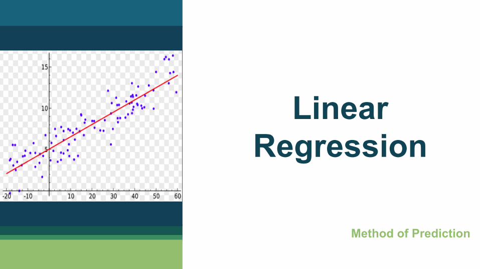
Linear Regression 1

Method of Prediction

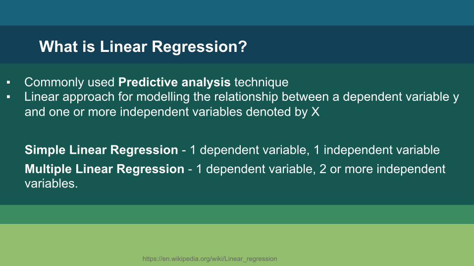
What is Linear Regression?

▪  Commonly used Predictive analysis technique ▪  Linear approach for modelling the relationship between a dependent variable y

and one or more independent variables denoted by X

Simple Linear Regression - 1 dependent variable, 1 independent variable Multiple Linear Regression - 1 dependent variable, 2 or more independent variables.

https://en.wikipedia.org/wiki/Linear_regression

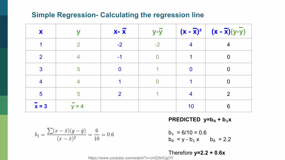
Simple Regression- Calculating the regression line

x y x- x y-y (x - x)² (x - x)(y-y)

1 2 -2 -2 4 4

2 4 -1 0 1 0

3 5 0 1 0 0

4 4 1 0 1 0

5 5 2 1 4 2

x = 3 y = 4 10 6

PREDICTED y=b₀ + b₁x

b₁ = 6/10 = 0.6 b₀ = y - b₁ x b₀ = 2.2 Therefore y=2.2 + 0.6x

https://www.youtube.com/watch?v=JvS2triCgOY

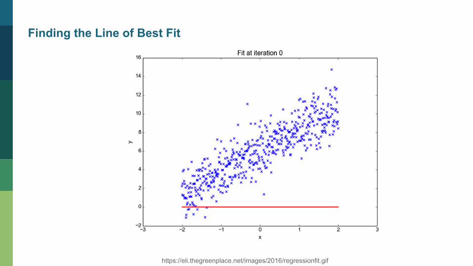
https://eli.thegreenplace.net/images/2016/regressionfit.gif

Finding the Line of Best Fit

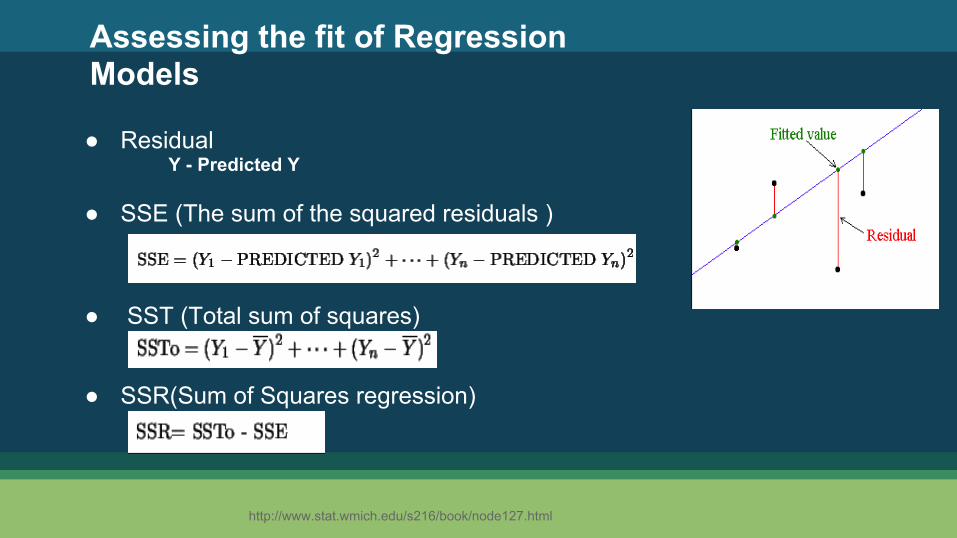
Assessing the fit of Regression Models

●  Residual

Y - Predicted Y ●  SSE (The sum of the squared residuals )

●  SST (Total sum of squares)

●  SSR(Sum of Squares regression)

http://www.stat.wmich.edu/s216/book/node127.html

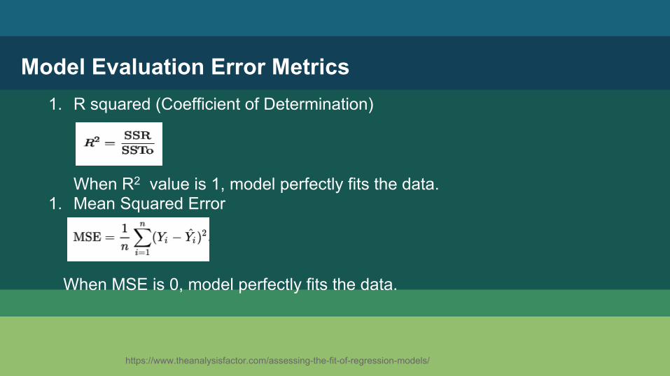
Model Evaluation Error Metrics 1.  R squared (Coefficient of Determination)

When R2 value is 1, model perfectly fits the data. 1.  Mean Squared Error

When MSE is 0, model perfectly fits the data.

https://www.theanalysisfactor.com/assessing-the-fit-of-regression-models/

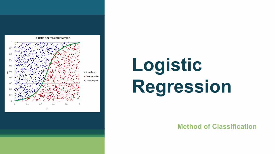
Logistic Regression

Method of Classification

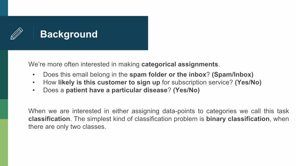
Background

We’re more often interested in making categorical assignments. ▪  Does this email belong in the spam folder or the inbox? (Spam/Inbox) ▪  How likely is this customer to sign up for subscription service? (Yes/No) ▪  Does a patient have a particular disease? (Yes/No)

When we are interested in either assigning data-points to categories we call this task classification. The simplest kind of classification problem is binary classification, when there are only two classes.

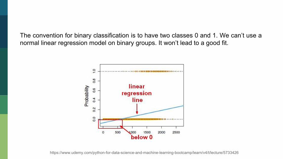
The convention for binary classification is to have two classes 0 and 1. We can’t use a normal linear regression model on binary groups. It won’t lead to a good fit.

https://www.udemy.com/python-for-data-science-and-machine-learning-bootcamp/learn/v4/t/lecture/5733426

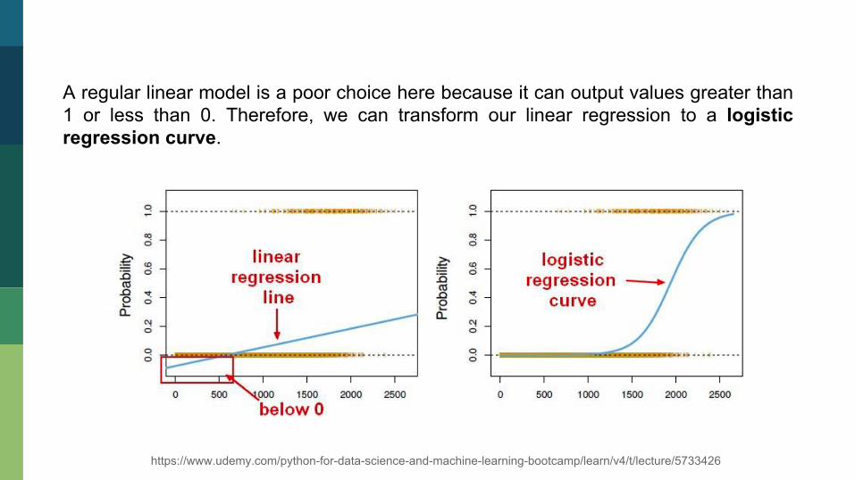
A regular linear model is a poor choice here because it can output values greater than 1 or less than 0. Therefore, we can transform our linear regression to a logistic regression curve.


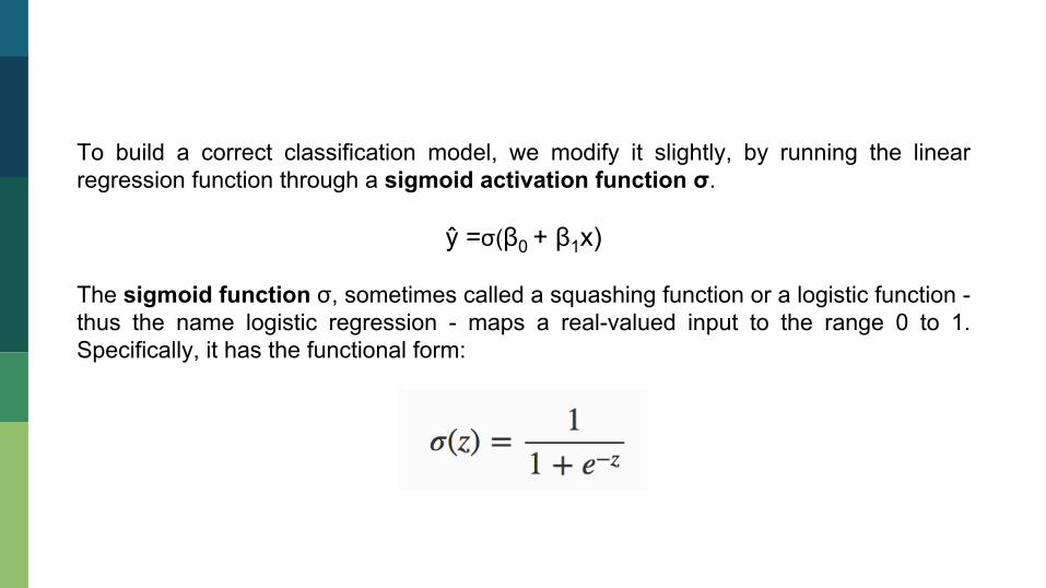
To build a correct classification model, we modify it slightly, by running the linear regression function through a sigmoid activation function σ.

ŷ =σ(β0 + β1x) The sigmoid function σ, sometimes called a squashing function or a logistic function - thus the name logistic regression - maps a real-valued input to the range 0 to 1. Specifically, it has the functional form:

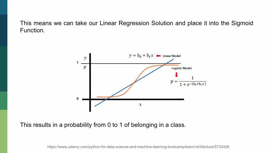
This means we can take our Linear Regression Solution and place it into the Sigmoid Function. This results in a probability from 0 to 1 of belonging in a class.


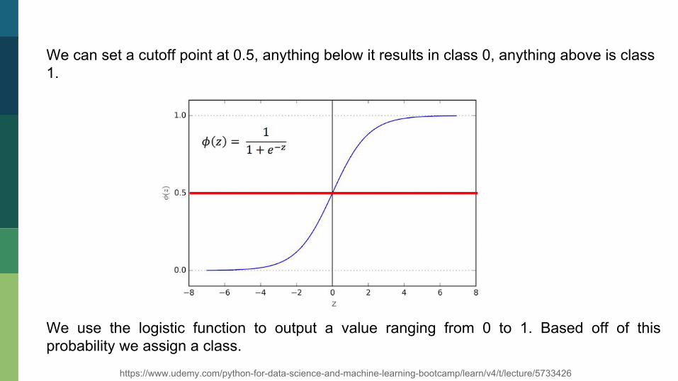
We can set a cutoff point at 0.5, anything below it results in class 0, anything above is class 1.

We use the logistic function to output a value ranging from 0 to 1. Based off of this probability we assign a class.

z


Model Evaluation

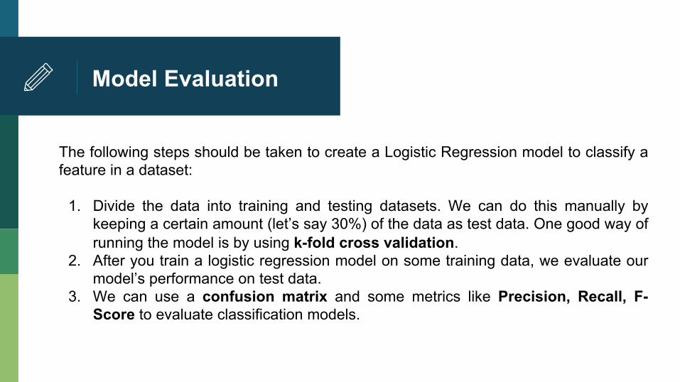
The following steps should be taken to create a Logistic Regression model to classify a feature in a dataset:

1.  Divide the data into training and testing datasets. We can do this manually by keeping a certain amount (let’s say 30%) of the data as test data. One good way of running the model is by using k-fold cross validation.

2.  After you train a logistic regression model on some training data, we evaluate our model’s performance on test data.

3.  We can use a confusion matrix and some metrics like Precision, Recall, F-Score to evaluate classification models.

Confusion Matrix

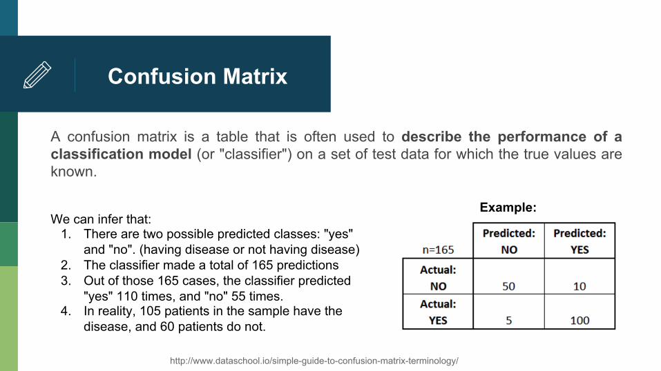
A confusion matrix is a table that is often used to describe the performance of a classification model (or "classifier") on a set of test data for which the true values are known.

We can infer that: 1.  There are two possible predicted classes: "yes"

and "no". (having disease or not having disease) 2.  The classifier made a total of 165 predictions 3.  Out of those 165 cases, the classifier predicted

"yes" 110 times, and "no" 55 times. 4.  In reality, 105 patients in the sample have the

disease, and 60 patients do not.

Example:

http://www.dataschool.io/simple-guide-to-confusion-matrix-terminology/

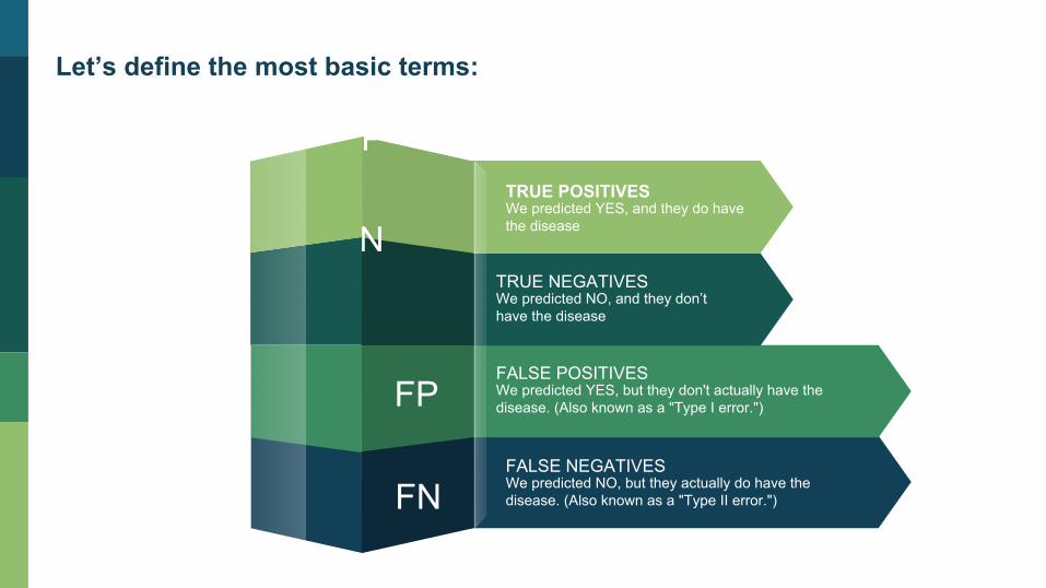
Let’s define the most basic terms:

TP

TN TRUE POSITIVES We predicted YES, and they do have the disease

FP

FN

TRUE NEGATIVES We predicted NO, and they don’t have the disease

FALSE POSITIVES We predicted YES, but they don't actually have the disease. (Also known as a "Type I error.")

FALSE NEGATIVES We predicted NO, but they actually do have the disease. (Also known as a "Type II error.")

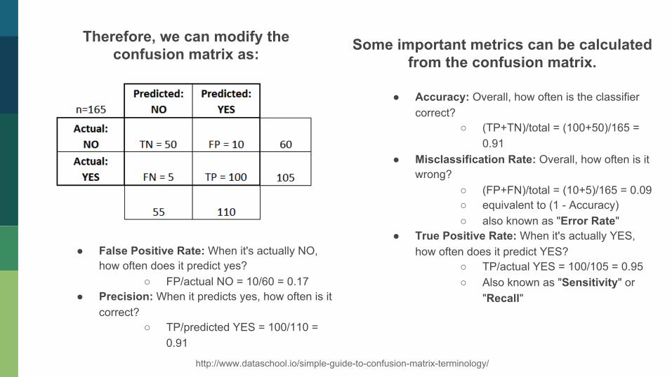
Therefore, we can modify the confusion matrix as:

Some important metrics can be calculated

from the confusion matrix.

●  Accuracy: Overall, how often is the classifier correct?

○  (TP+TN)/total = (100+50)/165 = 0.91

●  Misclassification Rate: Overall, how often is it wrong?

○  (FP+FN)/total = (10+5)/165 = 0.09 ○  equivalent to (1 - Accuracy) ○  also known as "Error Rate"

●  True Positive Rate: When it's actually YES, how often does it predict YES?

○  TP/actual YES = 100/105 = 0.95 ○  Also known as "Sensitivity" or

"Recall"

●  False Positive Rate: When it's actually NO, how often does it predict yes?

○  FP/actual NO = 10/60 = 0.17 ●  Precision: When it predicts yes, how often is it

correct? ○  TP/predicted YES = 100/110 =

0.91 http://www.dataschool.io/simple-guide-to-confusion-matrix-terminology/

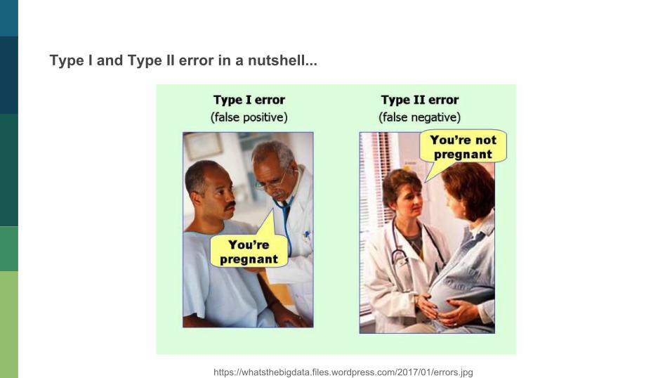
Type I and Type II error in a nutshell...

https://whatsthebigdata.files.wordpress.com/2017/01/errors.jpg

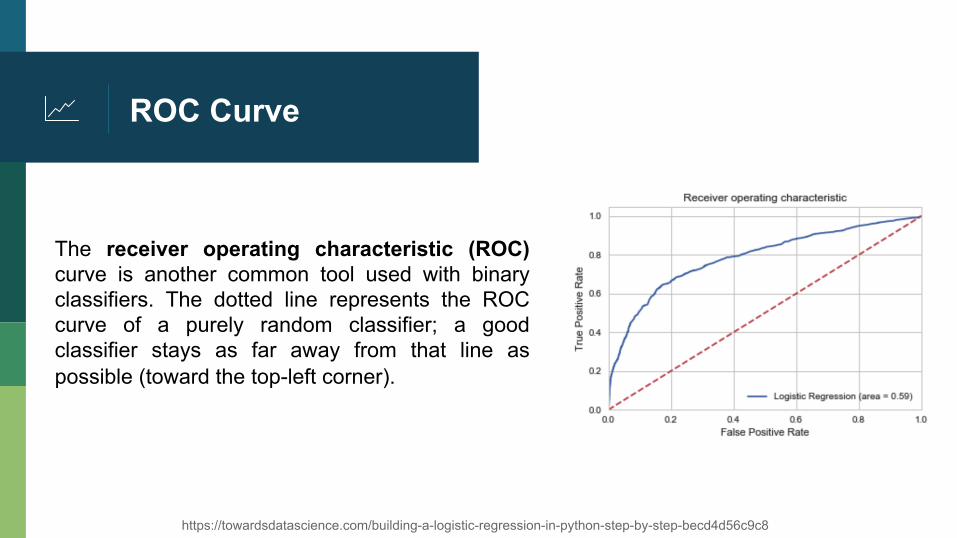
ROC Curve

The receiver operating characteristic (ROC) curve is another common tool used with binary classifiers. The dotted line represents the ROC curve of a purely random classifier; a good classifier stays as far away from that line as possible (toward the top-left corner).

https://towardsdatascience.com/building-a-logistic-regression-in-python-step-by-step-becd4d56c9c8

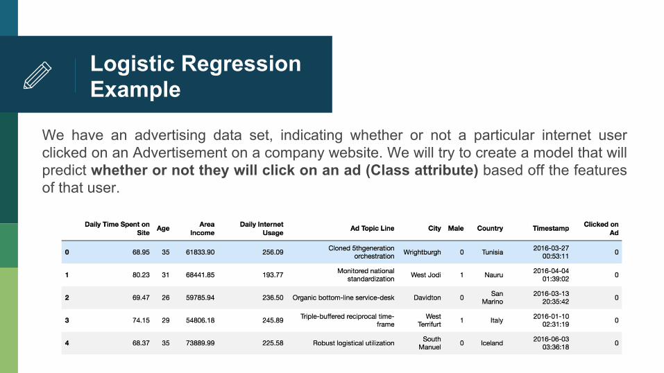
Logistic Regression Example

We have an advertising data set, indicating whether or not a particular internet user clicked on an Advertisement on a company website. We will try to create a model that will predict whether or not they will click on an ad (Class attribute) based off the features of that user.

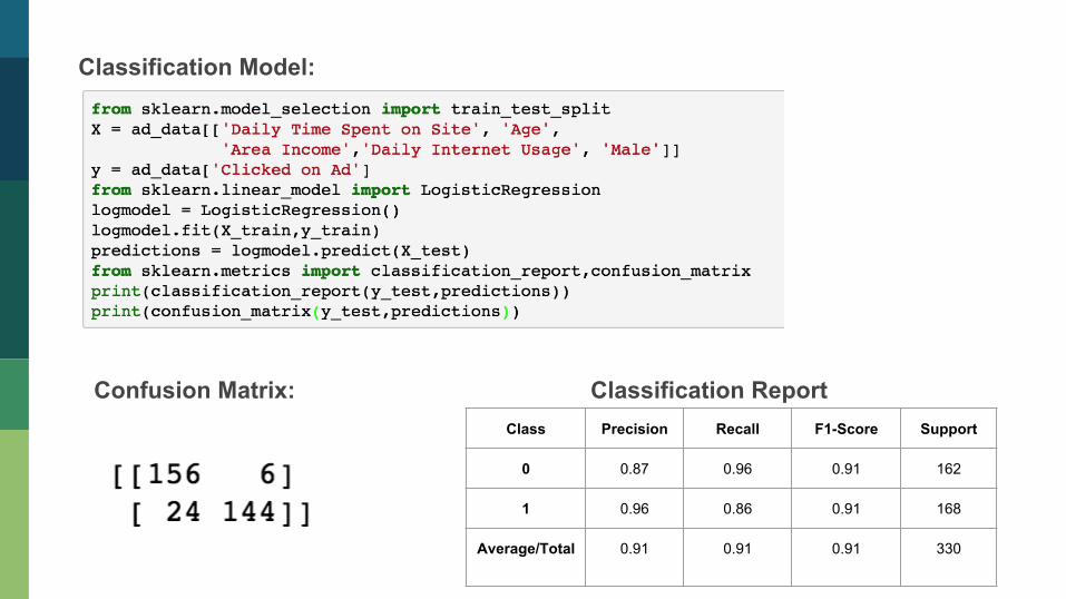
Classification Model:

Confusion Matrix: Classification Report Class Precision Recall F1-Score Support

0 0.87 0.96 0.91 162

1 0.96 0.86 0.91 168

Average/Total 0.91 0.91 0.91 330

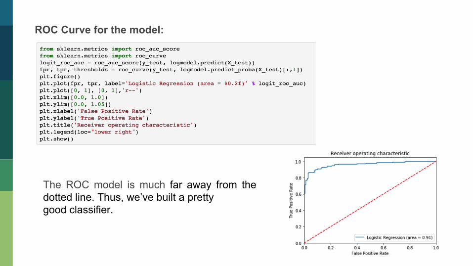
ROC Curve for the model:

The ROC model is much far away from the dotted line. Thus, we’ve built a pretty good classifier.

What about the Error?

http://memecaptain.com/gend_image_pages/-1PsXg

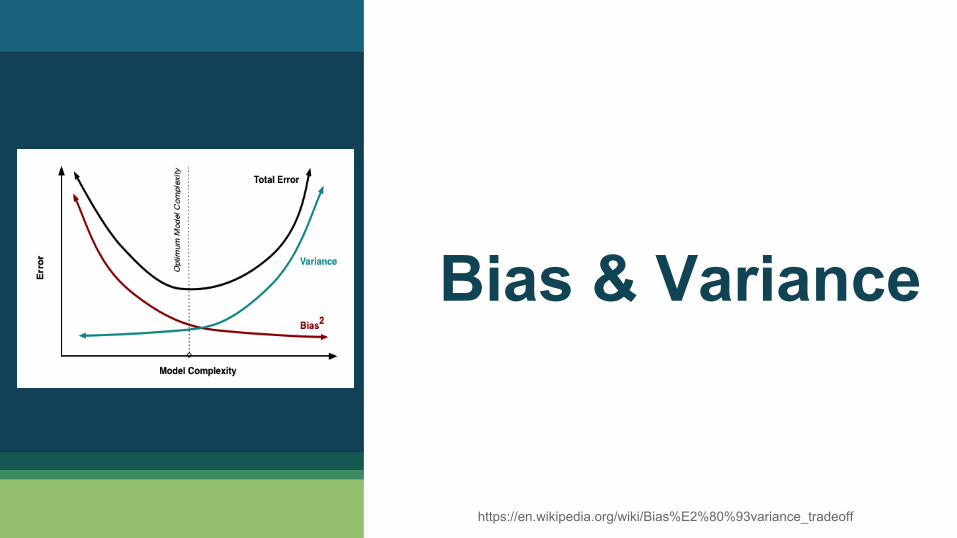
Bias & Variance

https://en.wikipedia.org/wiki/Bias%E2%80%93variance_tradeoff

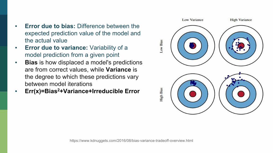
Bias Error ▪  Error due to bias: Difference between the

expected prediction value of the model and the actual value

▪  Error due to variance: Variability of a model prediction from a given point

▪  Bias is how displaced a model's predictions are from correct values, while Variance is the degree to which these predictions vary between model iterations

▪  Err(x)=Bias2+Variance+Irreducible Error

https://www.kdnuggets.com/2016/08/bias-variance-tradeoff-overview.html

Model Fit

https://en.wikipedia.org/wiki/Overfitting

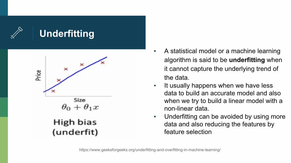
Underfitting ▪  A statistical model or a machine learning

algorithm is said to be underfitting when it cannot capture the underlying trend of the data.

▪  It usually happens when we have less data to build an accurate model and also when we try to build a linear model with a non-linear data.

▪  Underfitting can be avoided by using more data and also reducing the features by feature selection

https://www.geeksforgeeks.org/underfitting-and-overfitting-in-machine-learning/

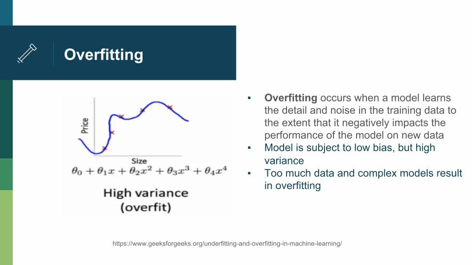
Overfitting

▪  Overfitting occurs when a model learns the detail and noise in the training data to the extent that it negatively impacts the performance of the model on new data

▪  Model is subject to low bias, but high variance

▪  Too much data and complex models result in overfitting


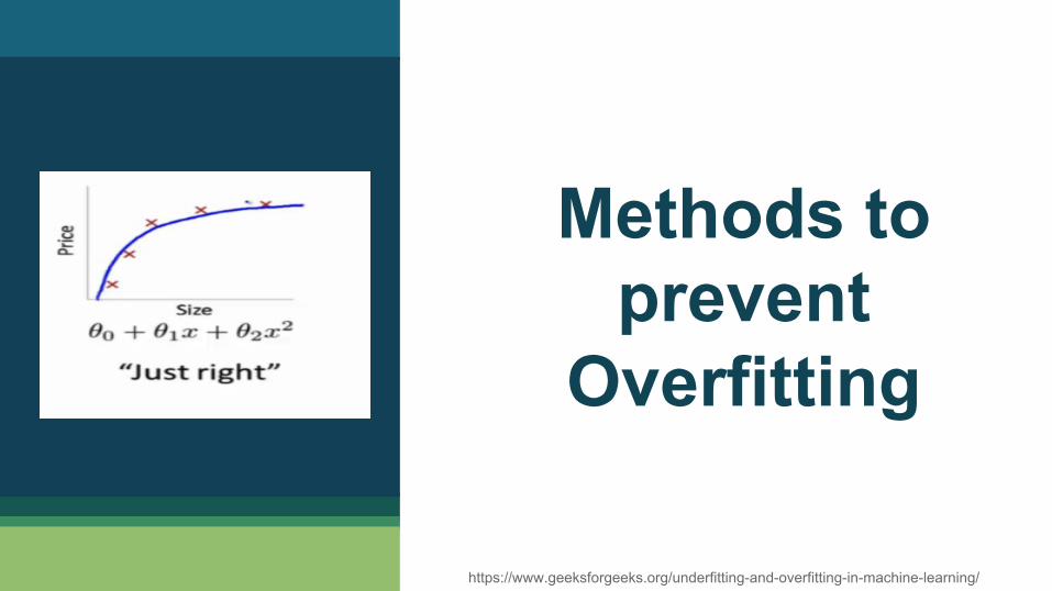
Methods to prevent

Overfitting


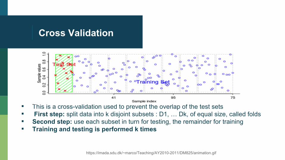
Cross Validation

▪  This is a cross-validation used to prevent the overlap of the test sets ▪  First step: split data into k disjoint subsets : D1, … Dk, of equal size, called folds ▪  Second step: use each subset in turn for testing, the remainder for training ▪  Training and testing is performed k times

https://imada.sdu.dk/~marco/Teaching/AY2010-2011/DM825/animation.gif

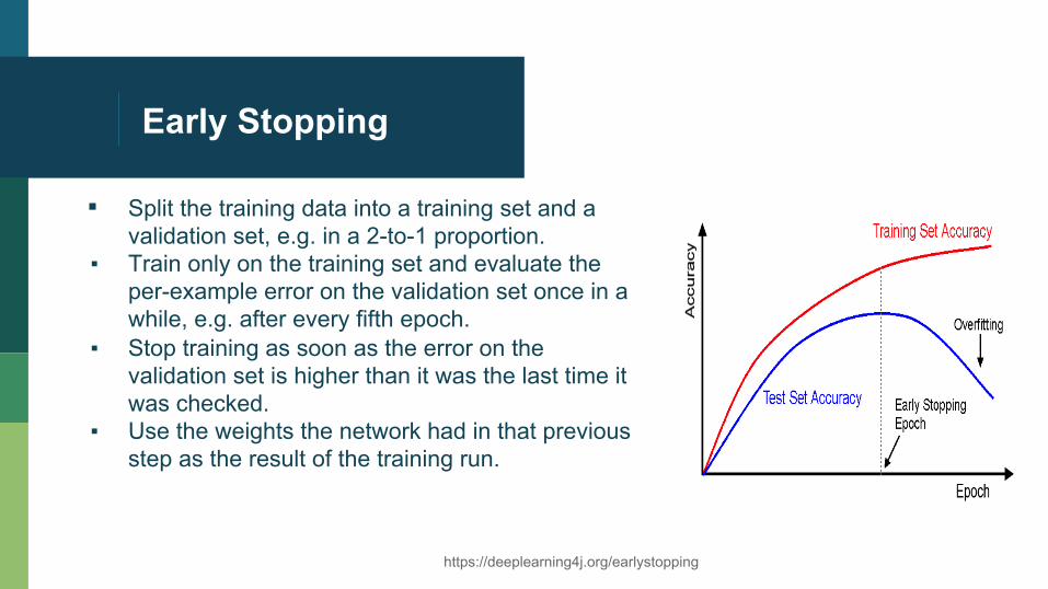
Early Stopping

▪  Split the training data into a training set and a validation set, e.g. in a 2-to-1 proportion.

▪  Train only on the training set and evaluate the per-example error on the validation set once in a while, e.g. after every fifth epoch.

▪  Stop training as soon as the error on the validation set is higher than it was the last time it was checked.

▪  Use the weights the network had in that previous step as the result of the training run.

https://deeplearning4j.org/earlystopping

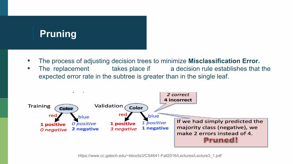
Pruning

▪  The process of adjusting decision trees to minimize Misclassification Error. ▪  The replacement takes place if a decision rule establishes that the

expected error rate in the subtree is greater than in the single leaf.

https://www.cc.gatech.edu/~bboots3/CS4641-Fall2016/Lectures/Lecture3_1.pdf

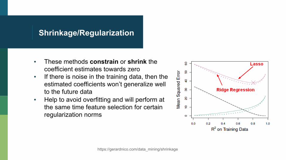
Shrinkage/Regularization

▪  These methods constrain or shrink the coefficient estimates towards zero

▪  If there is noise in the training data, then the estimated coefficients won’t generalize well to the future data

▪  Help to avoid overfitting and will perform at the same time feature selection for certain regularization norms

https://gerardnico.com/data_mining/shrinkage

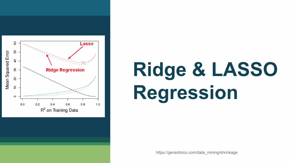
Ridge & LASSO Regression

https://gerardnico.com/data_mining/shrinkage

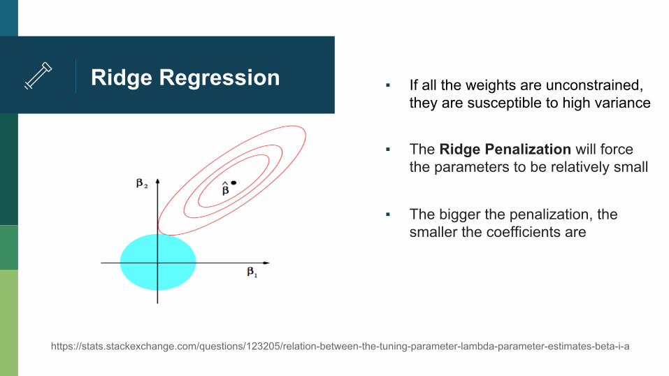
Ridge Regression ▪  If all the weights are unconstrained, they are susceptible to high variance

▪  The Ridge Penalization will force

the parameters to be relatively small ▪  The bigger the penalization, the

smaller the coefficients are

https://stats.stackexchange.com/questions/123205/relation-between-the-tuning-parameter-lambda-parameter-estimates-beta-i-a

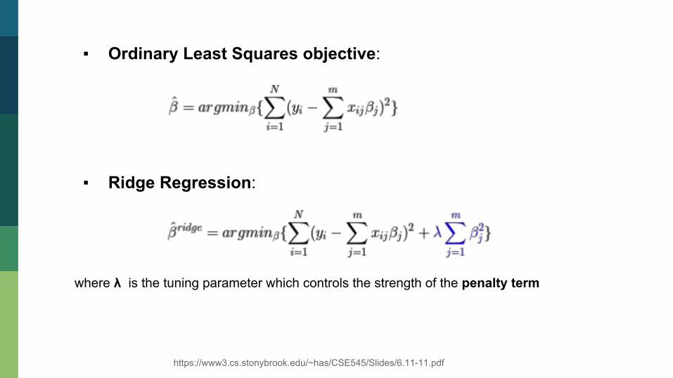
Bias Error ▪  Ordinary Least Squares objective:

▪  Ridge Regression:

where λ is the tuning parameter which controls the strength of the penalty term

https://www3.cs.stonybrook.edu/~has/CSE545/Slides/6.11-11.pdf

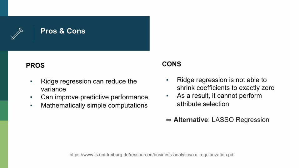
Pros & Cons

PROS ▪  Ridge regression can reduce the

variance ▪  Can improve predictive performance ▪  Mathematically simple computations

https://www.is.uni-freiburg.de/ressourcen/business-analytics/xx_regularization.pdf

CONS ▪  Ridge regression is not able to

shrink coefficients to exactly zero ▪  As a result, it cannot perform

attribute selection ⇒ Alternative: LASSO Regression

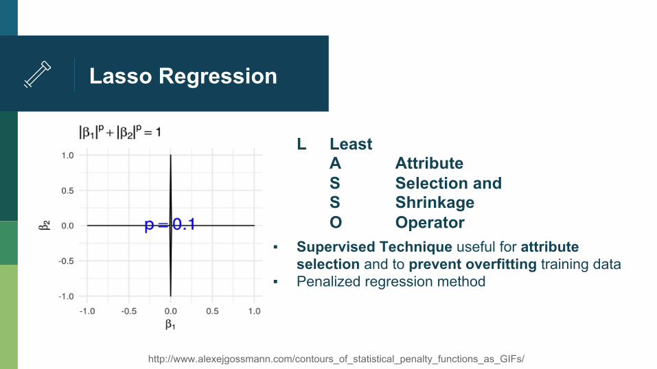
Lasso Regression

L Least A Attribute S Selection and S Shrinkage O Operator

▪  Supervised Technique useful for attribute selection and to prevent overfitting training data

▪  Penalized regression method

http://www.alexejgossmann.com/contours_of_statistical_penalty_functions_as_GIFs/

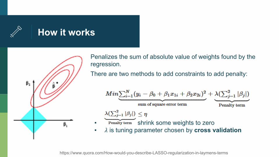
How it works

Penalizes the sum of absolute value of weights found by the regression. There are two methods to add constraints to add penalty:

▪  Constraints shrink some weights to zero ▪  𝜆 is tuning parameter chosen by cross validation

https://www.quora.com/How-would-you-describe-LASSO-regularization-in-laymens-terms

Properties & Advantages of LASSO

Properties ▪  Useful when number of classes is very less than number of attributes ▪  Makes the model sparser and reduces the possibility of overfitting

Advantages ▪  Improves the prediction accuracy and interpretability of regression models ▪  For feature selection, LASSO uses convex optimization to find best features. So,

it converges faster. ▪  Convenient when we want some automatic feature/variable selection

Application of Logistic Regression in the Study of

Students’ Performance Level

Paper Link

2 Miftar Ramosacaj, Dr. Vjollca Hasani, Dr. Alba Dumi

Journal of Educational and Social Research MCSER Publishing, Rome-

Italy, Vol. 5 No. 3 September 2015

Introduction

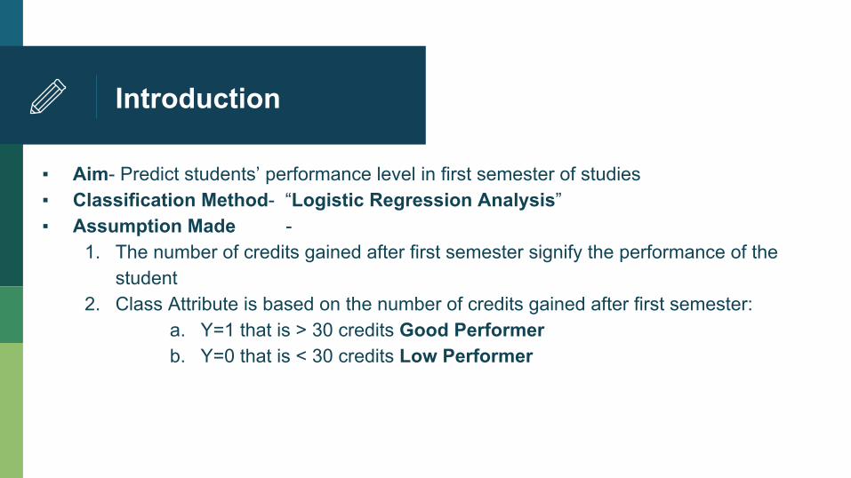
▪  Aim- Predict students’ performance level in first semester of studies ▪  Classification Method- “Logistic Regression Analysis” ▪  Assumption Made -

1.  The number of credits gained after first semester signify the performance of the student

2.  Class Attribute is based on the number of credits gained after first semester: a.  Y=1 that is > 30 credits Good Performer b.  Y=0 that is < 30 credits Low Performer

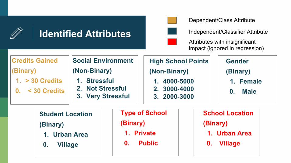
Identified Attributes

Gender (Binary)

1.  Female 0. Male

Type of School (Binary)

1.  Private 0. Public

High School Points (Non-Binary)

1.  4000-5000 2.  3000-4000 3.  2000-3000

Credits Gained (Binary)

1.  > 30 Credits 0. < 30 Credits

School Location (Binary)

1.  Urban Area 0. Village

Social Environment (Non-Binary)

1.  Stressful 2.  Not Stressful 3.  Very Stressful

Dependent/Class Attribute

Independent/Classifier Attribute

Attributes with insignificant impact (ignored in regression)

Student Location (Binary)

1.  Urban Area 0. Village

Class/Dependent Attribute Distribution

Data collected via Questionnaires filled by 240 Freshmen

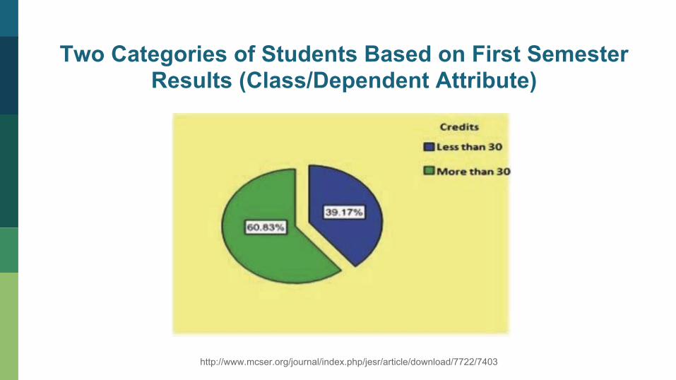
Two Categories of Students Based on First Semester Results (Class/Dependent Attribute)

http://www.mcser.org/journal/index.php/jesr/article/download/7722/7403

Few observations made on the Classifier

Attributes Data collected via Questionnaires filled by

240 Freshmen

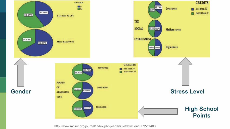
Gender

Stress Level

High School Points


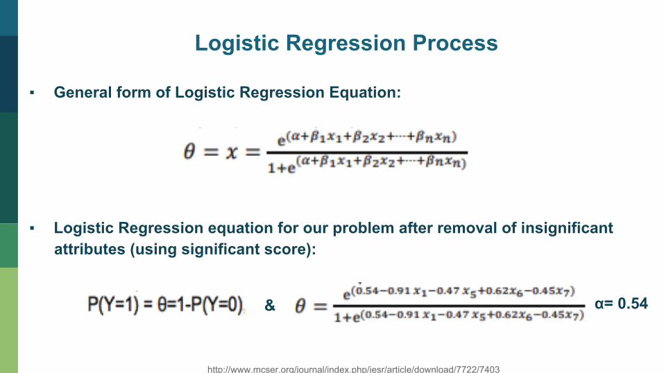
▪  General form of Logistic Regression Equation:

▪  Logistic Regression equation for our problem after removal of insignificant attributes (using significant score):


Logistic Regression Process

& α= 0.54

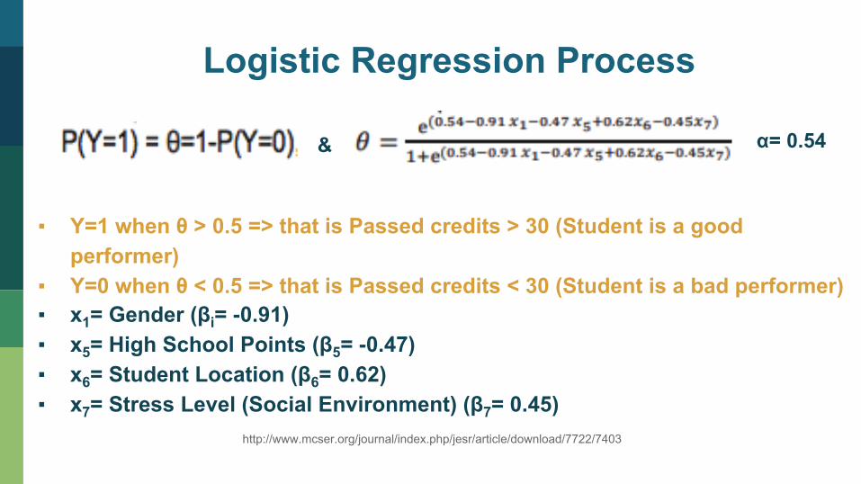
Logistic Regression Process

▪  Y=1 when θ > 0.5 => that is Passed credits > 30 (Student is a good performer)

▪  Y=0 when θ < 0.5 => that is Passed credits < 30 (Student is a bad performer) ▪  x1= Gender (βi= -0.91) ▪  x5= High School Points (β5= -0.47) ▪  x6= Student Location (β6= 0.62) ▪  x7= Stress Level (Social Environment) (β7= 0.45)


& α= 0.54

...What we want is a Machine that can Learn from experience… -Alan Turing (1947)

What was their conclusion? Was it good enough? Let’s look at some of their findings!

https://giphy.com/gifs/reaction-a5viI92PAF89q

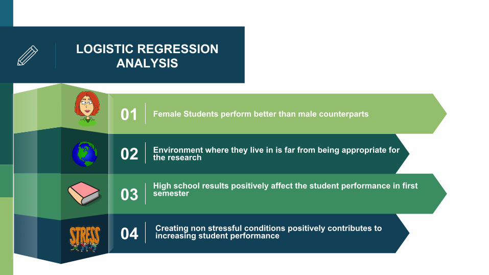
LOGISTIC REGRESSION ANALYSIS

01 Female Students perform better than male counterparts

02 Environment where they live in is far from being appropriate for the research

03 High school results positively affect the student performance in first semester

04 Creating non stressful conditions positively contributes to increasing student performance

statistical methods (regression)

Documents