Statistical methods research done as science ratherthan mathematics

James S. Hodges

Division of Biostatistics, University of Minnesota, Minneapolis, Minnesota USA 55414

email: hodge003@umn.edu

May 4, 2017

ABSTRACT

This paper is about the way we study statistical methods. As an example, it uses the

random regressions model, in which data come in clusters and the intercept and slope of

cluster-specific regression lines are treated as a bivariate random effect. Maximizing this

model’s restricted likelihood is prone to produce an estimate of −1 or +1 for the correlation

between the two random effects or of 0 for one of the random-effect variances. We argue that

this is a problem; that the problem lacks an explanation, not to mention a solution, because

our discipline has developed little understanding of how contemporary models and methods

map data into inferential summaries; that such understanding is absent, even for a model

as simple as random regressions, because of a near-exclusive reliance on mathematics as a

tool to gain understanding; and that judging from our literature, math alone is no longer

sufficient for this task. We then argue that as a discipline, we can and should add a tool

to our toolkit, breaking open our black-box methods by mimicking the five steps that our

colleagues in molecular biology commonly use to break open Nature’s black boxes: design

a simple model system, formulate hypotheses using that system, test them in experiments

on that system, iterate as needed to reformulate and test hypotheses, and finally test the

results in an “in vivo” system. We demonstrate this style of inquiry by using it to understand

conditions under which the random-regressions restricted likelihood is likely to be maximized

at a boundary value. Resistance to this empirical approach to gaining understanding seems

to arise from a view that it lacks the certainty or intellectual heft of mathematics, perhaps

because simulation experiments in our literature rarely do more than measure a new method’s

operating characteristics in a small range of situations. We argue that such work can make

useful contributions including, as in molecular biology, the findings themselves and sometimes

the designs used in the five steps; that these contributions have as much practical value as

mathematical results; and that therefore they merit publication as much as the mathematical

results our discipline esteems so highly.

1

1 Introduction: Why we should do science as well as

math to understand our methods

This paper is about how we study statistical methods, using as an example analyses that

employ a particular model. We begin by describing the latter, which leads to the former.

A random regressions model (as it’s called in some literature) is a common choice for

a situation in which observations are made in clusters and observation j in cluster i has

outcome yij that we would like to model as a linear function of a regressor xij. Ruppert et al

(2003, Section 4.2) give the example of weights measured for nine successive weeks on each of

48 young pigs: a pig is a cluster, pig i’s weight in week j is yij, and the regressor xij is week

number. In general, xij can be a vector; this paper considers scalar xij. Often it makes sense

to let the regression relationship vary between clusters as yij = β0i + β1ixij + εij, where εij is

an error term; in the example, β1i is pig i’s growth rate per week. If (β0i, β1i) is of interest and

clusters have small sample sizes, it can be advantageous to let clusters “borrow strength” from

each other by using a model like the following. For yij measured on a continuous scale, the εij

are modeled as independently and identically distributed (iid) N(0, σ2e) random variables and

the cluster-specific intercept-slope pairs are modeled as iid draws (β0i, β1i)′ ∼ N((b0, b1)

′,Σ).

In this paper, the 2× 2 covariance matrix Σ is parameterized as

Σ =

σ2c ρσcσs

ρσcσs σ2s

, (1)

where the subscripts “c” and “s” refer to the intercepts β0i and slopes β1i respectively. The

correlation ρ describes the association, across clusters, of β0i and β1i.

The conventional analysis of a mixed linear model like this begins by maximizing the re-

stricted likelihood (sometimes called the residual likelihood) to estimate (σ2e , σ

2c , σ

2s , ρ). The

estimates (σ2e , σ

2c , σ

2s , ρ) are then taken as given and estimates and tests for, e.g., (b0, b1) are

computed, so (σ2e , σ

2c , σ

2s , ρ) is central to the analysis. A Bayesian analysis adds prior dis-

tributions for (b0, b1) and (σ2e , σ

2c , σ

2s , ρ) to give posterior distributions and other summaries,

but problems afflicting the conventional analysis are still of interest because the restricted

likelihood, multiplied by a prior for (σ2e , σ

2c , σ

2s , ρ), is identical to the marginal posterior for

(σ2e , σ

2c , σ

2s , ρ) assuming a flat (improper) prior for (b0, b1). If (σ2

e , σ2c , σ

2s , ρ) also has a flat

prior, the marginal posterior is identical to the restricted likelihood.

The restricted-likelihood maximizing (σ2e , σ

2c , σ

2s , ρ) can be on the boundary of legal values,

i.e., ρ = −1 or +1, σ2c = 0, or σ2

s = 0; based on doing or supervising about 40 such analyses, it

often is. An informal observation is that when such inconvenient results occur, the restricted

likelihood is often quite flat, so that the data provide little information about (σ2e , σ

2c , σ

2s , ρ).

This implies that in a Bayesian analysis, the posterior differs little from the prior.

2

Is it a problem that ρ = −1 or +1 fairly readily in practice? Yes: In the pig-weight

example, if our estimate tells us the slope and intercept for each piglet are perfectly anti-

correlated in the population of pigs, this is obviously false. The defective estimate may be a

symptom of a problem with the conventional analysis or the model or experimental design

but it is nonetheless substantive nonsense and that is a problem.

Such estimates are also a problem because when they occur, standard software gives

useless or misleading information. It does so because as a discipline we have practically

no knowledge about why such estimates occur: there is, apparently, no literature on when

ρ = −1 or +1, and very little on estimates at boundaries more generally1. But perhaps this

hole in our theory is not really a problem: when an inconvenient estimate occurs, one can, for

example, examine the profiled log-likelihood or do a Bayesian analysis. Either alternative,

however, leaves us floating on the same sea of ignorance. If we consider how completely

single-error-term linear models are understood — they have produced no surprises since the

1980s2 — it is clear by contrast that our discipline has a shortage of understanding about how

contemporary methods, even simple ones like random regressions, map data into inferential

summaries. We need more understanding, not just more convenient software.

Why do we, as a discipline, have so little understanding of the methods we have created

and promote? Our primary tool for gaining understanding is mathematics, which has obvious

appeal: most of us trained in math and there is no better form of information than a theorem

that establishes a useful fact about a method. But the preceding sentence imposes a heavy

burden: it must be possible to prove a theorem and facts established by the theorem must

be useful. We find finite-sample facts indispensible because real datasets have finite samples

and asymptotic theorems never tell us how to apply their conclusions to finite samples. But

finite-sample theorems about contemporary methods are rare; it seems inescapable that they

are at least extremely difficult, given their popularity in earlier eras.

This paper considers a complementary tool for opening our black-box methods, modeled

explicitly on the approach molecular biologists use to open Nature’s black boxes.

Before doing so, it seems necessary to address our discipline’s prejudice in favor of math-

ematics and against such empirical approaches. Among statisticians, a common response to

our suggestion of the molecular-biology model of inquiry is to propose new formulations of

the random-regressions model, i.e., to try to turn it into a solvable math problem. While this

might be productive some day, random regressions is a simple model by today’s standard and

one can only speculate about whether such an effort will, in fact, produce anything useful

even for such a simple model.

Unfortunately, we statisticians either do not perform or do not publish purely empirical

1The entirety, it seems, of literature on zero variance estimates is discussed below.2S. Weisberg, personal communication, 2016.

3

studies. (If you doubt this, try to find empirical studies of the accuracy of standard approxi-

mations. Student literature reviews found 0 and 1 publications for logistic and Cox regression

respectively; Clifton 1997 and Huppler Hullsiek 1996.) The strength of this preference seems

odd given that our discipline exists to help others establish facts in situations in which the-

orems are impossible. The crux seems to be an implicit view that an empirical approach

to studying statistical methods lacks the certainty or intellectual heft to justify publication

alongside theorems. Perhaps this is not surprising: In the statistical theory used to train

us, hypotheses and measurement methods simply exist, when in fact creating them is a real

accomplishment (e.g., Kary Mullis’s 1993 Nobel prize in chemistry for making polymerase

chain reaction practical). Also, although many, perhaps most, statisticians spend their ca-

reers collaborating with scientists, unlike them we have not developed widely-accepted ways

of generalizing empirical findings from the specific cases included in experiments. (It was not

necessary, for example, to examine every kind of organism to conclude that the genetic code

was the same in all organisms.) Our dismissive attitude toward empirical studies is also

understandable given that in our literature, simulation experiments are rarely more than

obligatory but often perfunctory exercises in measuring operating characteristics of methods

too complex to permit exact theory, when in fact simulation experiments can be used to test

a great variety of hypotheses, as shown below.

As a matter of strategy, is our discipline or indeed an individual researcher better off do-

ing something relatively simple (the molecular-biological approach) and learning something

quickly, or betting on the ability to produce useful facts in the long run with mathematics?

A reasonable strategy would, it would seem, do some of each. The present paper suggests

that we can learn about contemporary black-box statistical methods by mimicking molecular

biology, demonstrates that approach, and argues that it makes contributions useful enough

to compete with theorems for space in our journals. Broadly, our colleagues in molecular

biology proceed by the following steps:

• Capture the phenomenon of interest in a simple model system, not a statistical model

but rather “a usually miniature representation of something” [Merriam-Webster’s on-

line dictionary], e.g., an animal or cell-culture model.

• Hypothesize about the phenomenon of interest in terms of the model system.

• Do experiments with the model system to test those hypotheses.

• Iterate, revising the model system and structure of hypotheses as needed.

• Test the revised hypotheses in a more realistic in vivo system.

This paper demonstrates this approach by using it to understand why maximizing the re-

stricted likelihood for a random-regressions model often gives boundary-value estimates.

4

We are certainly not the first to suggest studying statistical methods empirically. For

example, Larntz (1978) did extensive simulation experiments that established, among many

other things, the excessive conservatism of the usual rule of thumb for deciding whether

to use the chi-squared approximation for Pearson’s chi-squared test. Larntz’s student John

Adams (Adams 1990a, 1990b) did massive simulation experiments involving response-surface

methods, optimal design, and split-plot designs to produce a great variety of information

about linear regression methods, e.g., the effect of variable selection, outlier rejection, and

the Box-Cox method on the null distribution of the regression F-statistic. These studies were

carefully designed exercises in measuring operating characteristics; simulation experiments

testing explicit hypotheses are harder to find. Schapire (2013, 2015) described a series of

hypothesis-driven simulation experiments showing, among other things, that no available

theory (e.g., Friedman et al 2000) explains why AdaBoost works as well as it does and

fails when it does. (Schapire 2015, a talk in a memorial session for Leo Breiman, empha-

sized the hypotheses more than does Schapire 2013. Dr. Schapire avers [e-mail, 26 August

2015] that Prof. Breiman “very much advocated . . . an experimental approach to machine

learning/statistics” though we have not found a suitable citation.)

We emphatically do not claim to have the last word on how to study statistical methods

empirically, or to present an algorithm for conducting such studies, an idea that has long

since been discredited. (Feyerabend 1993 is just one example.) The results of an empirical

study are, of course, not as iron-clad as a theorem drawing the same conclusions but the odds

against producing such theorems are discouraging. This suggests that an orchard of low-

hanging fruit awaits if our discipline re-directs some energy away from asymptotic theorems

and toward this simple, productive approach.

Sections 2 through 6 describe and demonstrate the steps of the molecular-biology ap-

proach. The statistical-methods question is: In a random-regressions fit, which features of

the design or data-generating process influence the chance that the restricted likelihood is

maximized at ρ = ±1? Section 7 discusses the results and their implications for how we

study our methods. Each section discusses its step’s intellectual content; although the pri-

mary contribution of work in this approach will be the utility of the results, sometimes an

empirical study introduces a design of broader value that is itself a contribution. Details are

in the Supplement or are omitted; all are suitable for student exercises.

2 The model system

In biology, model systems include cell cultures and living organisms of complexity ranging

from bacteria to zebrafish to rodents to primates. For our example problem, the model

system is a simple random-regressions model specified as follows.

5

For clusters indexed by i, the data yij are presumed to arise as

yij = β0i + β1ixij + εij, i = 1, . . . , N, j = 1, . . . , s, (2)

where the εij are iid N(0, σ2e) independently of the (β0i, β1i)

′, which are iid N((b0, b1)′,Σ),

with Σ parameterized as in (1). The cluster size is s = 2m+ 1 for m a positive integer, so s

is odd. Given s, the regressor xij is stacked in a vector h taking the value

h = (−1,−(m− 1)/m, . . . , 0, . . . , (m− 1)/m, 1)′ (3)

so the range of the xij does not change with s. (This prevents some uninteresting artifacts.)

To put this in the usual mixed linear model notation y = Xβ + Zu + ε with cov(u) = G

and cov(ε) = R, let H be the s× 2 design matrix within a cluster, with orthogonal columns

1s, an s-vector of 1’s, and h as in (3). We have N clusters and n = Ns observations, and

X = 1N ⊗H is n× 2

β = (b0, b1)′ is 2× 1

Z = IN ⊗H is n× 2N

u = (u10, u11|u20, u21| . . . |uN0, uN1)′ is 2N × 1

G = BlockDiag(Σ) is 2N × 2N, and

R = σ2eIn,

(4)

where the observations in y are sorted first by cluster i and then by j within cluster, ⊗ is

the Kronecker product, defined as A⊗B = (aijB), “|” indicates matrix partitioning, and Id

is the d-dimensional identity matrix. In this notation, β0i = b0 + ui0 and β1i = b1 + ui1.

These features of the model system can be varied: the number of clusters N , the within-

cluster sample size s, and all unknowns. Nature presents us with (σ2e , σ

2c , σ

2s , ρ); sometimes,

at least, we can hope to manage the chance of ρ = ±1 by choosing the sample sizes N and

s. The simulation experiments below set (b0, b1)′ = (0, 0)′ without loss of generality because

this mean structure is removed from the data in computing the restricted likelihood.

What is this step’s intellectual content? The achievement in choosing a model system

(or a “simplest interesting case”) is to make it as simple as possible while still allowing

hypotheses of interest to be stated in the model’s terms and tested. In biology, the payoffs

of simplification are ability to control inputs to and measure outputs of the model system,

and to isolate the causal effects of factors manipulated in experiments. Simplification has a

cost, the need to hedge on interpretation; reviews of grant proposals and journal manuscripts

generally involve implicit negotiation about the limits of the model system. For studying

statistical methods, the payoffs of simplification are ability to do more explicit derivations

and simpler, faster computing, which permit hypotheses to be formulated and tested eco-

nomically in designed experiments. The cost is the risk of omitting an important feature

6

of the problem, though the final step (“test the revised hypothesis . . . ‘in vivo’”) provides

some protection against this risk. The model system above is simplified by having a single

regressor and forcing all clusters to have the same design matrix, with orthogonal columns.

These simplifications and others introduced below permit fairly explicit derivations while

retaining the ability to manipulate N , s, and (σ2e , σ

2c , σ

2s , ρ). As in biology, the key ques-

tions are whether the model system reproduces the phenomena of interest and whether it

behaves like the unsimplified system. We will see below that for the present model system

the answers are, respectively, “yes” and “as far as we can tell”.

For this model, the restricted likelihood is straightforward, so its derivation is omitted.

Define L to be s × (s − 2) with orthonormal columns satisfying L′1s = L′h = 0; L is used

to project onto the residual space within each cluster. Define W to be N × (N − 1) with

orthonormal columns such that W′1N = 0; W is used to project onto the between-cluster

residual space and its columns are contrasts in cluster-specific quantities. The log restricted

likelihood is then

−N(s− 2)

2log σ2

e −1

2σ2e

RSS (5)

−N − 1

2log det(F) − 1

2

N−1∑k=1

t′kF−1tk, (6)

where RSS = y′(IN ⊗ LL′)y (7)

and F = DΣD + σ2eI2 for D = diag(s, q)1/2,

where q = (2m2 + 3m+ 1)/3m and the 2× 1 vector tk = (W′k ⊗ [D−1H′])y for Wk the kth

column of W. Line (5) is a function only of σ2e and y; the quadratic form RSS in (5) is

the residual sum of squares from the unshrunk regressions within clusters, aggregated across

clusters. The unknowns (σ2c , σ

2s , ρ) appear only in (6), in which each tk is a contrast in the

unshrunk estimates of cluster-specific (β0i, β1i). The sum of quadratic forms in (6) is the

additional residual sum of squares arising from shrinkage for given (σ2e , σ

2c , σ

2s , ρ).

This form of the log restricted likelihood is about as simple as possible but it is still too

complicated to allow intuition: F is a function of all of σ2e , σ

2c , σ

2s , and ρ and the data enter

both (5) and (6) in complicated ways. This affects the next step in the biological model of

inquiry, generating hypotheses, to which we now turn.

3 Generating hypotheses

A necessary condition for the log restricted likelihood (henceforth log RL) or profiled log RL

to be maximized at ρ = −1 is that its derivative with respect to ρ, evaluated at ρ = −1,

is negative. This condition motivates deriving a predictor of ρ = −1 to use in generating

7

hypotheses, as follows: simplify the log RL, profile out one unknown, evaluate the derivative

of the profiled log RL with respect to ρ at ρ = −1, and finish with more simplifications. We

begin to deviate from a mathematical approach here by creating an approximation not to

replace the original expression but as an instrument for generating hypotheses. This grants

us a certain freedom: the predictor’s utility lies not in its accuracy as an approximation but

rather in the frequency with which simulation experiments support the hypotheses it helps

us generate, and this utility is exhausted when the hypotheses are tested.

The first simplification is to let σ2c = σ2

s ≡ σ2r . Real problems can be made close to this

by scaling xij, so this seems like a small sacrifice in generality. The log RL now has three

unknowns, σ2r , σ

2e , and ρ; we reduce that to two by profiling out σ2

r . Define r = σ2e/σ

2r so

that σ2e = rσ2

r . It is easy to show that the maximizing value of σ2r given (r, ρ) is

σ2r(r, ρ) = (Ns− 2)−1{RSS/r +

N−1∑k=1

t′k(σ2rF−1)tk}; (8)

note that σ2rF−1 is a notational convenience and is not in fact a function of σ2

r . Ignoring

unimportant constants, the profiled log RL is then

−N(s− 2)

2log r − N − 1

2log{(s+ r)(q + r)− sqρ2} (9)

−Ns− 2

2log{RSS/r +

N−1∑k=1

t′k(σ2rF−1)tk}.

The derivative of (9) with respect to ρ at ρ = −1 is messy and permits little intuition.

Therefore, we simplified the derivative by replacing functions of the data with their expected

values under the model. Specifically, we replaced r/RSS by (N(s − 2)σ2r)−1 and, defining

tk = (tkc, tks)′, we replaced t2kc by σ2

r(s+ r), t2ks by σ2r(q + r), and tkctks by

√sqσ2

rρ, yielding

this predictor of when ρ = −1:(Ns−N − 1

(1 + r/s)(1 + r/q)

)1−(

Ns− 2

Ns−N − 1

) 1− N−1N(s−2)ρ

1 + 2(N−1)N(s−2)

(1+r/s)(1+r/q)+ρ(1+r/s)(1+r/q)−1

, (10)

a function of N , s, ρ, and r but not σ2r . This can be understood as a 0th order Taylor

expansion around the expected values of functions of the data. (It is easy to derive a very

similar predictor for ρ = +1, which is given in the Supplement and used below.)

We seek to understand when the derivative of the log RL (5) with respect to ρ at ρ = −1

is negative; we derived the predictor (10) to generate hypotheses about when that derivative

is negative. However, it’s easy to show that the predictor is positive for all finite N and s,

all ρ ∈ (−1, 1), and all finite positive r. (The proof is in the Supplement.) Thus (10) fails as

an approximation to the derivative of the profiled log RL, but as we’ll see in the simulation

experiments, it does well at predicting when ρ = −1: as (10) becomes smaller (closer to

8

zero), ρ is more likely to be −1 and as (10) becomes larger, ρ is less likely to be −1. Thus

it is accurate to describe (10) as a predictor of the event ρ = −1.

We now exercise the predictor (10) as a function of N , s, ρ, and r to generate hypotheses

about what promotes or suppresses ρ = ±1. The following facts about the predictor of

ρ = −1 are easy to prove (proofs are in the Supplement):

• Given N , s, and ρ, as r increases — i.e., as the error variance σ2e increases relative to

the random-effect variance σ2r — the predictor goes to zero.

• Given ρ and r, as either N or s increases, the predictor increases.

• Given N , s, and r, as ρ goes to −1, the predictor goes to zero.

Combined with the hypothesis that a small predictor value implies a high chance that ρ = −1

and a large predictor value implies a small chance that ρ = −1, these facts give three hypothe-

ses about ρ’s behavior. If these hypotheses are correct — and the simulation experiments

support them — then ρ = −1 becomes more likely as the error variance increases relative

to the intercept and slope variances and less likely as either sample size increases. This

implies that ρ = ±1 is mainly a consequence of poor resolution in the study design, with

“resolution” used in the same sense as the resolution of a measuring device or video monitor,

i.e., error variation is large and is not suppressed by sample size. (The tiny literature about

zero variance estimates is consistent with this. For the balanced one-way random effects

model, an estimate of zero for the between-groups variance arises from poor resolution; see

Hill 1965, Section 3B. Hodges 2014, Chapter 18 extends Hill 1965 and shows an example

suggesting that the same is true for mixed-effects analysis of variance more generally.)

To develop quantitative hypotheses about how N , s, ρ, and r affect the chance of ρ = −1,

we drew 1000 sets of (N, s, ρ, r) by making independent draws of each quantity and computed

the common (base 10) log of the predictor for each such set. Each quantity was drawn iid,

N from {50, 150, 250, . . . , 1050}, s from {5, 15, 25, . . . , 105}, ρ from {−0.9,−0.8, . . . ,−0.1},and log10 r from {−2,−1.6,−1.2, . . . , 2}. The resulting design in (N, s, ρ, r) was roughly

balanced. (Real datasets we have analyzed as random regressions had cluster counts and

sizes at the low ends of these ranges of N and s.) Analyzing these log10 predictor values

using ANOVA with factors N , s, ρ, and r, the main effects for r, s, N , and ρ had mean

squares 172.5, 23.0, 5.3, and 2.0 respectively; the two-way interactions ρ-by-r and s-by-r had

mean squares 0.08 and 0.01 respectively; and the other four two-way interactions and the

combined three- and four-way interactions each had mean squares less than 2× 10−5. Thus

the main effects dominate the behavior of log10 predictor.

Figure 1a shows the effects of N and s marginal to (i.e., averaging over) the other factors;

its vertical axis is SAS’s least-squares means in an analysis treating N , s, ρ, and r as

9

●

●

●

●

●

●

●●

●●

●

2.5

3.0

3.5

4.0

4.5

5.0

N

fitte

d lo

g10(

pred

icto

r)

50 250 450 650 850 1050

5 15 25 35 45 55 65 75 85 95 105

s

●

●

●

●

●

●

●

●

●

●

●

N

s

(a)

●

●

●

●

●

●

●

●

●

●

●

−2 −1 0 1 2

02

46

8

log10(r)

fitte

d lo

g10(

pred

icto

r)

●

●

●

●

●

●

●

●

●

●

●

●

●

●

●

●

●

●

●

●

●

●

r main effect

rho = −0.9

rho = −0.1

(b)

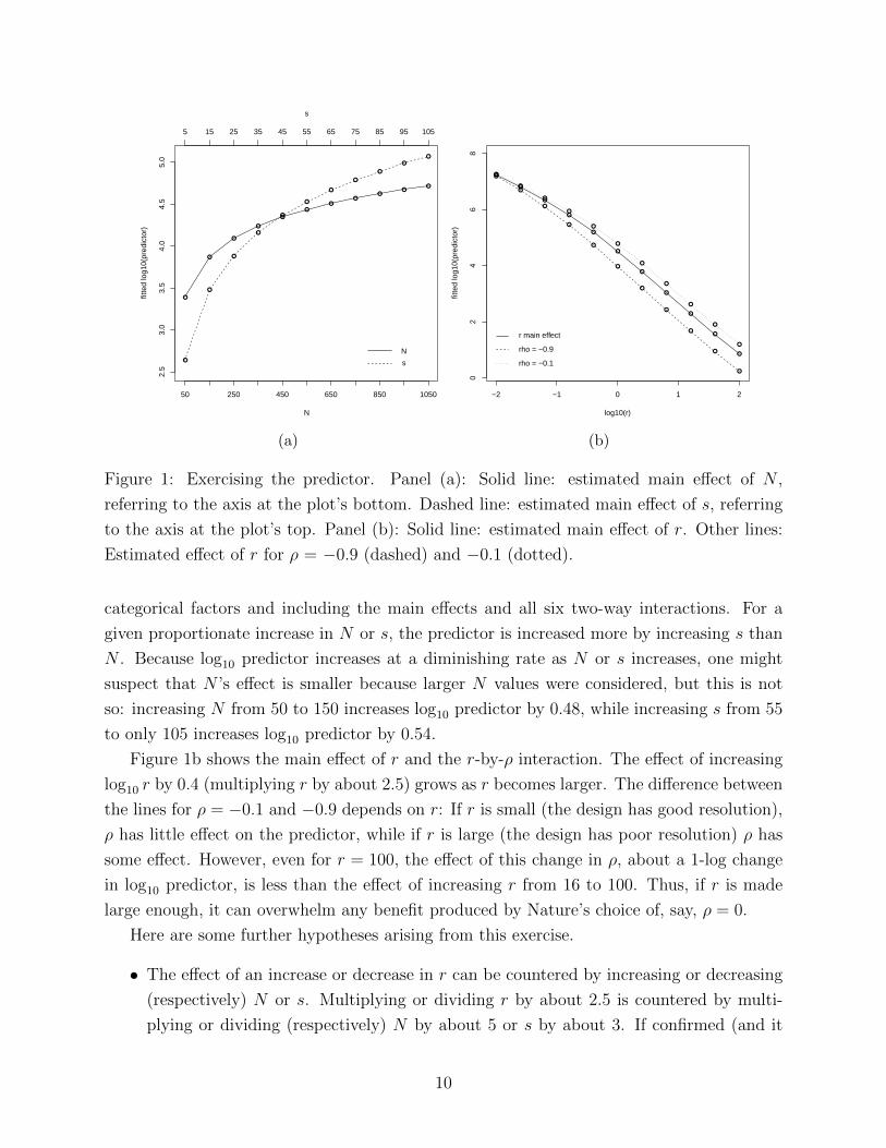
Figure 1: Exercising the predictor. Panel (a): Solid line: estimated main effect of N ,

referring to the axis at the plot’s bottom. Dashed line: estimated main effect of s, referring

to the axis at the plot’s top. Panel (b): Solid line: estimated main effect of r. Other lines:

Estimated effect of r for ρ = −0.9 (dashed) and −0.1 (dotted).

categorical factors and including the main effects and all six two-way interactions. For a

given proportionate increase in N or s, the predictor is increased more by increasing s than

N . Because log10 predictor increases at a diminishing rate as N or s increases, one might

suspect that N ’s effect is smaller because larger N values were considered, but this is not

so: increasing N from 50 to 150 increases log10 predictor by 0.48, while increasing s from 55

to only 105 increases log10 predictor by 0.54.

Figure 1b shows the main effect of r and the r-by-ρ interaction. The effect of increasing

log10 r by 0.4 (multiplying r by about 2.5) grows as r becomes larger. The difference between

the lines for ρ = −0.1 and −0.9 depends on r: If r is small (the design has good resolution),

ρ has little effect on the predictor, while if r is large (the design has poor resolution) ρ has

some effect. However, even for r = 100, the effect of this change in ρ, about a 1-log change

in log10 predictor, is less than the effect of increasing r from 16 to 100. Thus, if r is made

large enough, it can overwhelm any benefit produced by Nature’s choice of, say, ρ = 0.

Here are some further hypotheses arising from this exercise.

• The effect of an increase or decrease in r can be countered by increasing or decreasing

(respectively) N or s. Multiplying or dividing r by about 2.5 is countered by multi-

plying or dividing (respectively) N by about 5 or s by about 3. If confirmed (and it

10

is), this hypothesis has a design implication: for a given increase in total sample size,

increasing s causes a greater reduction in the chance that ρ = −1 than increasing N .

• Changes in ρ induce smaller changes in the chance that ρ = −1 than do changes in r,

N , or s; some changes in r have effects so large that no change in ρ can counter them.

In particular, if r is large enough then for any ρ, ρ is very likely to be −1.

As for this step’s intellectual content, hypothesis generation is one of the central creative

activities of scientific work and a key difference between competent and brilliant scientists is

that the latter pose more fruitful and penetrating hypotheses. The ability to produce deep,

powerful hypotheses depends on insight and creative manipulation of the method under

study. Molecular biologists can now generate and test hypotheses by manipulating their

objects of study, e.g., by creating gene-knockout organisms; we can generate hypotheses

by manipulating our objects of study, which are combinations of equations and algorithms,

using approximations as above.

The mathematical approach to studying statistical methods does include hypotheses; they

are called unproven conjectures and rarely see the light of day unless they are proven, while

disproofs of scientific hypotheses are routinely published. If empirical study of statistical

methods became more common, it might not be appropriate for journal articles to describe

the hypothesis-generation step at length, as we have, or perhaps to describe it at all but its

importance cannot be denied.

4 Testing the hypotheses using simulation experiments

With hypotheses in hand, the next step is to design and execute experiments to test them.

To derive the predictor, we set σ2c = σ2

s and in the simulation experiments below, we sim-

ulated data by setting σ2c = σ2

s . The goal, however, is to understand the log LR-maximizing

estimates for the unsimplified random-regressions model, in which σ2c and σ2

s can be differ-

ent. Thus, although the hypotheses were stated above in terms of a single variance σ2r for

both the random intercept and random slope, and thus in terms of r = σ2e/σ

2r , and data

generation in the experiments below has σ2c = σ2

s , this restriction was not enforced in fitting

the models.

We did preliminary simulations to determine predictor values that are “on the cusp”,

i.e., (N, s, ρ, r) having these predictor values give some but not too many bad estimates,

where a “bad” estimate3 is ρ = ±1 or σ2c = 0 or σ2

s = 0. This is the region of (N, s, ρ, r) in

which changes in these inputs can affect the fraction of bad estimates, so it is most useful

for testing the hypotheses. Beginning this way mimicks our colleagues in biology: they

3We use this word at the risk of offending readers because it is short and, as argued above, appropriate.

11

select experimental settings so that their model system’s response is middling and thus most

readily changed by manipulating inputs.

The experiments are in three groups: one testing whether increasing r, the ratio of the

error variance to the random-effect variances, produces a large fraction of bad estimates; one

examining the tradeoffs between r on the one hand and N , s, and ρ on the other hand; and

a final set examining the effect of ρ. We present these three sets of experiments in turn.

The methods for the experiments were as follows.

• Datasets were simulated from (2) to (4) with β = (0, 0)′ and σ2c = σ2

s = 1 (with one

exception to the latter, noted below). Counts of simulated datasets in each experiment

are given with the results.

• Analyses were done in R (v. 3.1.2, R Core Team 2014) using the lmer function (lme4

package v. 1.1-7, Bates et al 2014). In preliminary experiments, lmer always found

a local maximum in constrast to various options in the nlme package, which failed

sometimes for large r. The variances σ2c and σ2

s were not forced to be equal in the fit.

• Results of experiments are summarized by presenting the values of N , s, ρ, and r defin-

ing each experimental setting, the predictors for −1 and +1, the percent of estimates

ρ = −1,+1, and NaN (“not a number” in R; i.e., σ2c = 0 or σ2

s = 0), and the sum of

these three percents, i.e., the percent of bad estimates.

4.1 Increasing r produces bad estimates

Table 1 shows results from Experiments A and B, which were done specifically for this

hypothesis though other experiments (below) support the same conclusion, especially Ex-

periment G. We used N = 500 and s = 21 in these experiments, values quite a bit larger than

in any real dataset to which we have fit a random regressions model. In both experiments,

as r increases, the predictor decreases and the percent of simulated datasets yielding bad

estimates increases. Datasets giving ρ = NaN had σ2c = 0 in all cases examined.

The difference between Experiments A and B is the value of ρ used in simulating the

data. Some might conjecture that the chance of a bad estimate is minimized by setting ρ = 0

while the chance of ρ = −1 would be reduced by setting ρ close to +1; Experiments A and

B (respectively) use these ρ. In these experiments, setting ρ close to +1 has no effect on

the chance of ρ = −1 for the two largest r values (settings 4 and 5) and only a slight effect

for setting 3. However, setting ρ close to +1 does give a much higher chance of ρ = +1 in

settings 1 and 2, and thus increases the chance of a bad estimate for those settings.

(In generating data for these experiments, r was made large by fixing σ2c = σ2

s = 1 and

making σ2e large but r could also be made large by fixing σ2

e and making σ2c and σ2

s small.

12

Table 1: Simulation experiments: Increasing r increases the chance of a bad estimate. 100

datasets per setting.

Experiment A predictor % with ρ

setting N s ρ r -1 +1 -1 +1 NaN Bad

1 500 21 0 101 3.6e+2 3.6e+2 0 0 0 0

2 500 21 0 102 6.4e+0 6.4e+0 11 7 1 19

3 500 21 0 103 8.0e–2 8.0e–2 21 33 30 84

4 500 21 0 104 8.2e–4 8.2e–4 19 29 40 88

5 500 21 0 105 8.2e–6 8.2e–6 15 36 32 83

Experiment B predictor % with ρ

setting N s ρ r -1 +1 -1 +1 NaN Bad

1 500 21 0.95 101 6.8e+2 1.5e+1 0 25 0 25

2 500 21 0.95 102 1.3e+1 2.6e–1 0 54 3 57

3 500 21 0.95 103 1.5e–1 3.1e–3 17 31 29 77

4 500 21 0.95 104 1.6e–3 3.2e–5 22 37 31 90

5 500 21 0.95 105 1.6e–5 3.2e–7 21 36 29 86

We re-did Experiments A and B with all settings identical except that σ2e was fixed at 1

and σ2c and σ2

s were set to give the desired r. The results, with 400 simulated datasets per

setting, were indistinguishable from those in Table 1.)

Experiment A gives the first hint of an oddity that recurs in later experiments: With

ρ = 0 and large r, we would expect ρ = +1 and ρ = −1 to be about equally likely, but in

fact ρ = +1 is rather more likely. In each of Experiments A and B, combining settings 3,

4, and 5, the fractions of datasets with ρ = +1 tests higher than the fraction with ρ = −1

(P < 0.001 in a two-tailed test).

4.2 Trading off r against N , s, and ρ

Table 2 shows Experiments C through F, which have the same structure: Setting 1 is a

base case chosen to give some bad estimates; in setting 2, r is changed; and settings 3, 4,

and 5 attempt to reverse the effect of setting 2’s change in r by changing only N , s, or ρ

respectively. In Experiments C, E, and F, setting 2 had a larger r than in setting 1, giving

more bad estimates; in Experiment D, setting 2 had a smaller r than in setting 1, giving

fewer bad estimates. For setting 2, r was either larger or smaller by a factor of about 2.5

13

(100.4) compared to setting 1, and N , s, and ρ in settings 3, 4, and 5 were chosen to make

the predictor of ρ = −1 as similar as possible to its value in setting 1. (Sometimes setting

4’s predictor value could not hit the target because s must be odd and at least 3.)

Experiments C and D used N and s that seem moderate though they are larger than in

any dataset we’ve analyzed. Experiment E has small N and large s; Experiment F has large

N and small s. We chose ρ = −0.8 for setting 1 in all experiments because in applications,

ρ < 0 is usually more plausible than ρ > 0: when the average slope in xij is positive, clusters

with low intercepts have more room to increase (and thus larger slopes) than do clusters

with high intercepts, and analogously when the average slope in xij is negative.

The chosen N and s counter the change in r more or less as predicted. In these four

experiments, a test comparing setting 3 vs. setting 1 (i.e., does the change in N counter

the change in r?) gives a large (non-significant) P-value except for Experiment E, where

the increase in N compensates more than predicted. Similarly, a test comparing setting

4 vs. setting 1 (i.e., does the change in s counter the change in r?) gives a large (non-

significant) P-value in all four experiments. The proportional changes in s that counter an

experiment’s change in r were 2.8, 3, 2.5, and 3 in Experiments C, D, E, and F respectively;

the corresponding proportional changes in N were 5, 4.8, 5.2, and 5.4.

A bigger surprise is the effect of changes in ρ, examined further in the following subsection.

4.3 The effect of ρ

The predictor predicted that a large change in ρ, from −0.8 to 0 in Experiments C, E, and

F, will counter an increase in r. But this change in ρ did not simply reduce the chance that

ρ = −1, though it did that; it also increased the chance that ρ = +1 or NaN (σ2c = 0 or

σ2s = 0). In Experiments C, E, and F, setting 5 with ρ increased from −0.8 to 0 produced

fewer datasets with ρ = −1 than settings 3 and 4 but this change in ρ did not predictably

counter changes in the chance of any kind of bad estimate: sometimes it overcompensated

and sometimes it undercompensated.

Experiment G, summarized in Table 3, further explores the effect of ρ. All settings have

the same fairly large N and s. Each block of 5 settings has one value of r and includes ρ

ranging from −0.95 to +0.95. For the relatively small r = 53, ρ behaves as one might expect:

when ρ = −0.95, 45% of the datasets have ρ = −1, when ρ = +0.95, 47% of the datasets

have ρ = +1, and intermediate ρ give intermediate results. However, as r increases this tidy

pattern dissolves so that when r = 3,000 or 100,000, the true ρ does not matter: ρ = −1 is

about equally likely for all ρ, as are ρ = +1 and NaN.

Experiment G’s results also show the oddity noted about Experiments A and B: When r

is large, so we would expect ρ = −1 and ρ = +1 to occur about equally often, in fact ρ = +1

is rather more frequent. In Experiment G’s settings 11 through 20, ρ = +1 occurs not quite

14

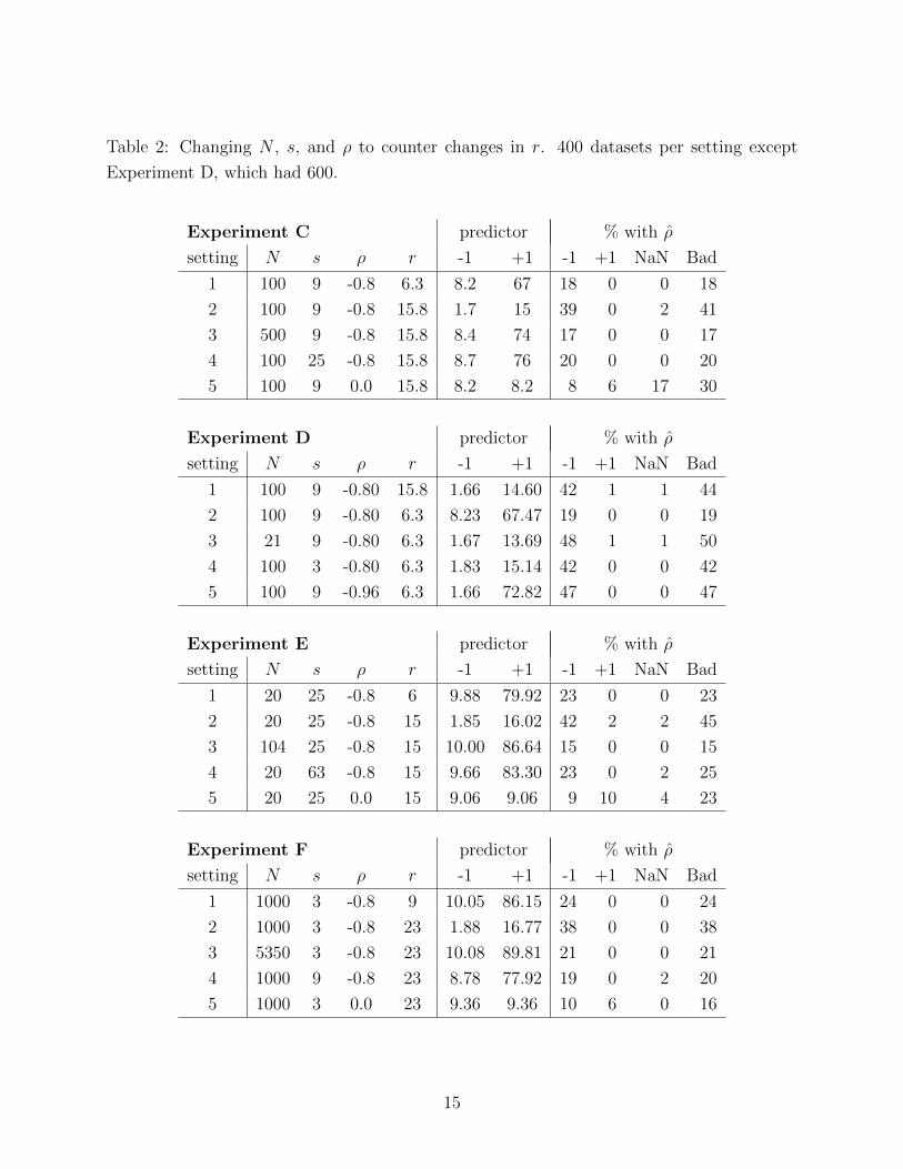
Table 2: Changing N , s, and ρ to counter changes in r. 400 datasets per setting except

Experiment D, which had 600.

Experiment C predictor % with ρ

setting N s ρ r -1 +1 -1 +1 NaN Bad

1 100 9 -0.8 6.3 8.2 67 18 0 0 18

2 100 9 -0.8 15.8 1.7 15 39 0 2 41

3 500 9 -0.8 15.8 8.4 74 17 0 0 17

4 100 25 -0.8 15.8 8.7 76 20 0 0 20

5 100 9 0.0 15.8 8.2 8.2 8 6 17 30

Experiment D predictor % with ρ

setting N s ρ r -1 +1 -1 +1 NaN Bad

1 100 9 -0.80 15.8 1.66 14.60 42 1 1 44

2 100 9 -0.80 6.3 8.23 67.47 19 0 0 19

3 21 9 -0.80 6.3 1.67 13.69 48 1 1 50

4 100 3 -0.80 6.3 1.83 15.14 42 0 0 42

5 100 9 -0.96 6.3 1.66 72.82 47 0 0 47

Experiment E predictor % with ρ

setting N s ρ r -1 +1 -1 +1 NaN Bad

1 20 25 -0.8 6 9.88 79.92 23 0 0 23

2 20 25 -0.8 15 1.85 16.02 42 2 2 45

3 104 25 -0.8 15 10.00 86.64 15 0 0 15

4 20 63 -0.8 15 9.66 83.30 23 0 2 25

5 20 25 0.0 15 9.06 9.06 9 10 4 23

Experiment F predictor % with ρ

setting N s ρ r -1 +1 -1 +1 NaN Bad

1 1000 3 -0.8 9 10.05 86.15 24 0 0 24

2 1000 3 -0.8 23 1.88 16.77 38 0 0 38

3 5350 3 -0.8 23 10.08 89.81 21 0 0 21

4 1000 9 -0.8 23 8.78 77.92 19 0 2 20

5 1000 3 0.0 23 9.36 9.36 10 6 0 16

15

Table 3: If r is big enough, ρ doesn’t matter. 400 datasets per setting.

Experiment G

predictor % with ρ

setting N s ρ r -1 +1 -1 +1 NaN Bad

1 500 21 -0.95 53 1.00 38.65 45 0 7 52

2 500 21 -0.50 53 9.96 29.78 10 0 10 20

3 500 21 0.00 53 19.89 19.89 3 1 1 5

4 500 21 0.50 53 29.78 9.96 0 12 1 13

5 500 21 0.95 53 38.65 1.00 0 47 1 48

6 500 21 -0.95 271 0.05 1.94 45 8 11 64

7 500 21 -0.50 271 0.50 1.50 30 17 15 62

8 500 21 0.00 271 1.00 1.00 23 27 9 58

9 500 21 0.50 271 1.50 0.50 13 40 8 61

10 500 21 0.95 271 1.94 0.05 6 52 5 64

11 500 21 -0.95 3000 4.4e-4 1.7e-2 23 30 31 83

12 500 21 -0.50 3000 4.4e-3 1.3e-2 21 33 30 84

13 500 21 0.00 3000 8.9e-3 8.9e-3 22 31 31 83

14 500 21 0.50 3000 1.3e-2 4.4e-3 22 34 29 84

15 500 21 0.95 3000 1.7e-2 4.4e-4 20 35 25 80

16 500 21 -0.95 1e+5 4.0e-7 1.6e-5 21 31 33 85

17 500 21 -0.50 1e+5 4.0e-6 1.2e-5 22 35 27 84

18 500 21 0.00 1e+5 8.0e-6 8.0e-6 18 32 32 82

19 500 21 0.50 1e+5 1.2e-5 4.0e-6 23 36 31 89

20 500 21 0.95 1e+5 1.6e-5 4.0e-7 21 33 31 85

16

1.5 times as often as ρ = −1, even when the true ρ is −0.95. Section 7 discusses this further.

4.4 The intellectual content of simulation experiments

In the United States, most health-care research funding comes from the National Institutes

of Health (NIH) and junior faculty are routinely coached about writing NIH proposals. One

maxim is that a proposal must be “hypothesis-driven” because a proposal for descriptive

research will surely fail. We think this exclusive emphasis is mistaken; in a new research

area, descriptive research is essential (e.g., how many people, and which people, have this

disease?). We academic statisticians, however, go too far in the other direction so that our

simulation experiments almost always describe operating characteristics of procedures and

rarely test hypotheses.

The distinction between hypothesis-driven and descriptive research is arguably artificial.

Does the stereotypical simulation describe or compare the new and old methods? But posing

explicit hypotheses about statistical methods — hypotheses other than “the new method has

the correct size and higher power than the old method” — suggests experimental designs dif-

fering from the stereotype. As a widely-read history of molecular biology put it, “Attractive

ideas, after all, are cheap and much of the stuff of scientific genius is devising tests” (Judson

1979), for example, Meselson and Stahl’s method for separating macromolecules according

to buoyant density, which made it possible to verify aspects of Watson and Crick’s DNA

model (see also Holmes 2001). Our own little experiments, above, are much like those of our

collaborators in biology and required no great imagination; those in Schapire (2013, 2015)

required considerably more. Perhaps we statisticians do not see the creativity in a good

simulation experiment because we have made such limited use of them.

5 Iterate: We haven’t asked quite the right question

The hypotheses to be tested were:

1. As the predictor of ρ = −1 becomes closer to zero, ρ is more likely to be −1; as the

predictor becomes larger, ρ is less likely to be −1.

2. Given N , s, and ρ, as r increases, ρ is more likely to be −1.

3. Given ρ and r, as either N or s increases, ρ is less likely to be −1.

4. Given N , s, and r, as ρ approaches −1, ρ is more likely to be −1.

5. The effect of an increase or decrease in r can be countered by an increase or decrease

(respectively) in N or s.

17

6. Multiplying or dividing r by about 2.5 is countered by multiplying or dividing (respec-

tively) N by a factor of about 5 or s by a factor of about 3.

7. Changes in ρ have a smaller effect on the chance that ρ = −1 than do changes in N

or s. In particular, if r is large enough, for any ρ, ρ is very likely to be ±1.

No result in Section 4 contradicts any of Hypotheses 1 through 4, though for large enough

r, the true value of ρ doesn’t matter, in the range tested. Experiments C, D, E, and F are

consistent with Hypotheses 5 and 6. The experimental results generally are consistent with

the second part of Hypothesis 7 (“if r is large enough . . . ”). As for the first part of Hypothesis

7 — “Changes in ρ have a smaller effect on the chance that ρ = −1 than do changes in N

or s” — the experimental results can be interpreted as meaning “you asked the question

poorly”. With further thought, it seems that the question that motivated this inquiry —

what conditions make it likely that ρ = −1? — was a red herring.

Experiments C through F were designed to examine how N , s, ρ, and r affect the chance

that ρ = −1, and setting 5 in these experiments stands out because it is the only setting

with much chance that ρ = +1 or NaN (i.e., σ2c = 0 or σ2

s = 0). However, in experiments A,

B, and G, with large values of r, ρ = −1 was less likely than either ρ = +1 or NaN. Reducing

the resolution of a design, in the sense of increasing σ2e , increases the chance of all kinds of

bad estimate, not just ρ = −1. The disease, it seems, is poor resolution; the different kinds

of bad estimate are merely different symptoms and all improve with the same treatment,

i.e., larger s or N or smaller σ2e .

This, and the fact that Section 3’s predictor has fulfilled its purpose and can now be

retired, prompted a final simulation experiment to estimate the probability of a bad estimate

as a function of N , s, ρ, and r. As in Section 3, we considered all combinations of N ∈{50, 150, 250, . . . , 1050}, s ∈ {5, 15, 25, . . . , 105}, ρ ∈ {−0.9,−0.8, . . . ,−0.1}, but for this

final experiment log10 r took values in {0, 0.4, 0.8, . . . , 4}. (It turns out that the values of

log10 r considered in Section 3 were small enough that few combinations of N , s, ρ, and r

had substantial probability of a bad estimate. This may explain some of Section 4’s results

regarding ρ.) For each of the resulting 11× 11× 9× 11 = 11, 979 settings, we simulated and

analyzed 40 datasets using the lmer function, as in Section 4.

For the binary outcome “bad estimate? (yes/no)”, treating each of N , s, ρ, and r as

a categorical factor, the four main effects and three two-way interactions involving r are

far larger than all the other interactions. Figure 2 shows interaction plots for the two-way

interactions involving r. In each panel, the horizontal axis is log10 r, the vertical axis is the

percent of simulated datasets giving a bad estimate, and from top to bottom, the panels show

a separate line for each level of N , s, and ρ respectively. Each plotted point is the percent of

11× 9× 40 = 3960 simulated datasets in the plots for N and s, and of 11× 11× 40 = 4840

18

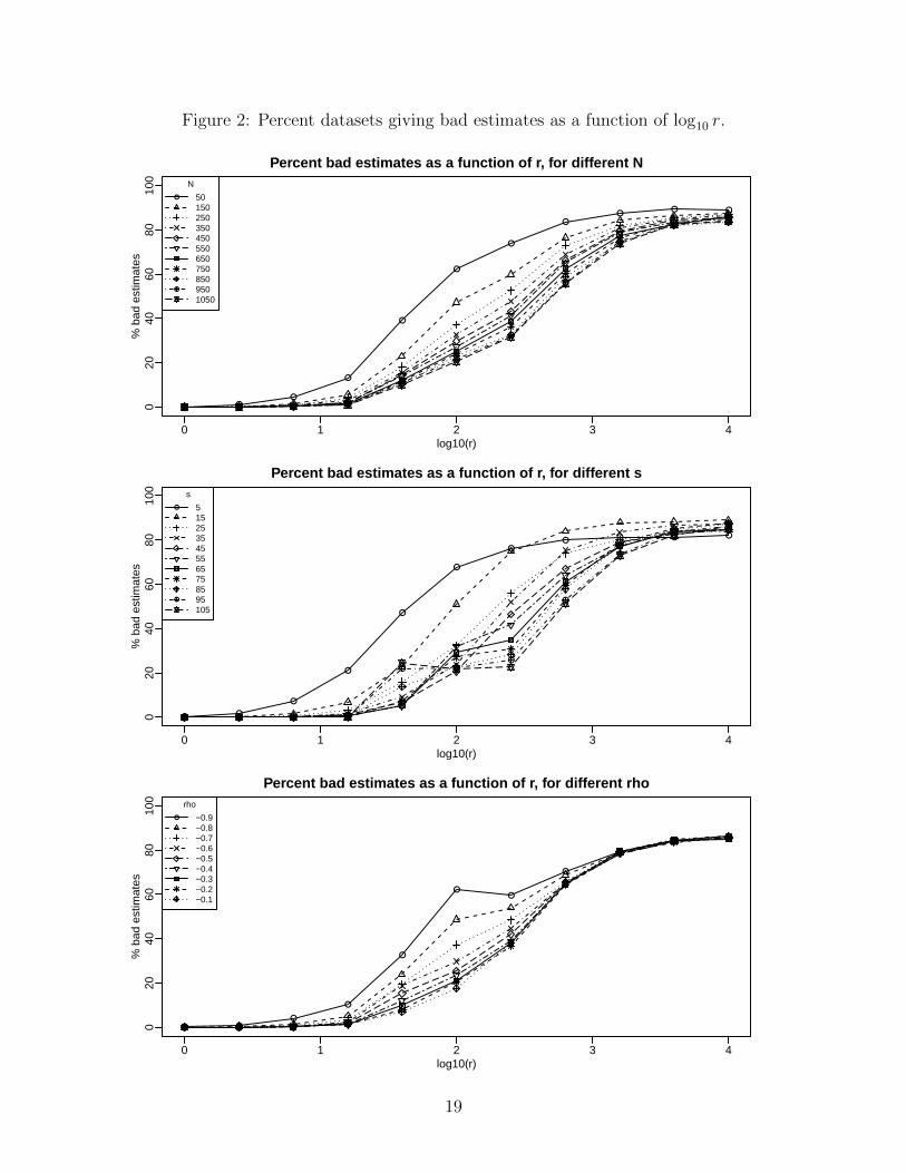
Figure 2: Percent datasets giving bad estimates as a function of log10 r.

0 1 2 3 4

020

4060

8010

0Percent bad estimates as a function of r, for different N

log10(r)

% b

ad e

stim

ates

● ●●

●

●

●

●

●●

● ●

● ● ● ●

●

●

●

●

●

●●

●

●

N

501502503504505506507508509501050

0 1 2 3 4

020

4060

8010

0

Percent bad estimates as a function of r, for different s

log10(r)

% b

ad e

stim

ates

● ●

●

●

●

●

●● ● ● ●

● ● ● ●

● ●●

●

●

●●

●

●

s

5152535455565758595105

0 1 2 3 4

020

4060

8010

0

Percent bad estimates as a function of r, for different rho

log10(r)

% b

ad e

stim

ates

● ●●

●

●

●●

●

●

●●

●

rho

−0.9−0.8−0.7−0.6−0.5−0.4−0.3−0.2−0.1

19

simulated datasets in the plot for ρ. Each plotted point has Monte Carlo standard error less

than 0.8 percentage points.

When r is large or small enough, the other factors have little effect on the chance of a

bad estimate. For middling r, N ’s effect is simple (Figure 2 top): increasing N reduces the

chance of a bad estimate. The same is true of ρ (Figure 2 bottom), though oddly r’s effect

is not monotonic for ρ = −0.9. Figure 2’s middle panel has a surprise: For log10 r = 1.6

and 2.0, the effect of s is not monotonic, nor is it for large r. If we consider ρ = ±1 and

ρ = NaN (i.e., σ2c = 0 or σ2

s = 0) as distinct outcomes, plots analogous to Figure 2 (in the

Supplement) show that the irregularities in Figure 2 middle arise almost entirely from ρ =

NaN, while ρ = ±1 behave much more regularly. This is a kind of competing risks situation

in that a given dataset can have only one of four possible outcomes: a “good” estimate,

ρ = −1, ρ = +1, or ρ = NaN; ρ = NaN behaves most oddly as a function of N , s, ρ, and r

and because these outcomes compete, this induces oddities in results for the other outcomes.

As in the biological research we are mimicking, rich results lead to new questions. For

the present purpose of demonstration, this is a good place to stop.

In the theory used to teach us, a hypothesis is stated and tested and the story ends.

This may be a useful way to formulate math problems for developing statistical tools but

it does not describe scientific practice. Experiments designed to test particular hypotheses

often motivate a reformulation of those hypotheses or a larger structure of hypotheses and

this reformulation may be the most important result of a collection of experiments. Perhaps

it is not appropriate for a scientific report to show the intermediate steps leading to that

all-important reformulation, but the present paper is intended to demonstrate an approach

to statistical methods research, not to present a model for scientific reports arising from it.

6 An “in vivo” experiment

The last step in many molecular-biology projects is to test all or part of the studied effect in

a larger model, moving from cell cultures to mice or from rodents to larger mammals. The

object is to see if the effects found in the simple model system can be reproduced in a more

complex organism. In the random-regressions example, the analog is to see if effects from

the experiments can be reproduced in a less constrained situation. The following “in vivo”

experiment fits a model to a real dataset and then constructs artificial datasets from the fit

by inflating the estimated errors εij, to see whether inflating the error variance (increasing

r) produces bad estimates as it did in the simple model system.

The dataset is the HMO data analyzed in Hodges (1998) and re-analyzed by Wakefield

(1998) and Davison (1998), available at http://www.biostat.umn.edu/∼hodges/RPLMBook/

Datasets/09 HMO premiums/Ex9.html. The outcome yij is the individual health-plan pre-

20

mium for plan j in state i, for i = 1, . . . , 45 and j = 1, . . . , ni, where the ni are described

below. The total number of plans is∑i ni = 341. Filling the role of xij is the common

logarithm of the number of families enrolled in plan (i, j). The model fit to the data is:

yij = b0 + b1(log10 families enrolled)ij + [1, (log10 families enrolled)ij](ui0, ui1)′

+ b0E (average expenses per admission)i + b0N(New England indicator)i + εij(11)

where (b0, b1), (ui0, ui1), and εi,j are defined as above, (average expenses per admission)iis state i’s average expenses per hospital admission, (New England indicator)i indicates

whether state i is in the New England region, and b0E and b0N are scalar coefficients.

The first row of (11) contains the population-average intercept and slope in log families

enrolled and the corresponding bivariate random effect. Except for the intercept, right-

hand-side variables are standardized: the plan-level variable “log10 families enrolled” was

centered and scaled using the average and standard deviation across the 341 plans; the state-

level variables were centered and scaled using the average and standard deviation across

states. (Before standardizing, the New England indicator was coded as +1 for states in

New England and −1 for other states.) A fit using the function lmer gave point estimates

(b0, b1, b0E, b0N) = (180,−2.21, 4.78, 16.1) and (ρ, σ2e , σ

2c , σ

2s) = (0.115, 487, 97.7, 5.39).

This model and dataset differ in several ways from the model system in earlier sections:

• The fit has non-zero estimates for (b0, b1) and has other fixed effects.

• Within-state sample sizes vary: ni ranges from 1 to 31 with median 5 and average 7.6.

• The state-specific design matrices differ between states with no particular pattern.

• The regressor “log10 families enrolled” was not scaled to make σ2c ≈ σ2

s ; σ2c and σ2

s

differ by more than an order of magnitude.

• The analyses cited above suggest that εij is modestly right-skewed and has a higher

variance in a few states.

Artificial datasets were constructed by taking the fit to the actual data, multiplying the

residuals from that fit by φ ≥ 1, and adding the inflated residuals to the fit. The artificial

datum y(φ)ij was defined as

y(φ)ij = fitij + φεij

where εij = yij − fitij

and fitij = b0 + b1(log10 families enrolled)ij + [1, (log10 families enrolled)ij](ui0, ui1)′

+ b0E (average expenses per admission)i + b0N (New England indicator)i,

(12)

21

Table 4: “In vivo” simulation experiment: Increasing the error variance produces a bad

estimate; increasing it more produces a different kind of bad estimate.

φ ρ σ2e σ2

e/φ2 σ2

c σ2s

1.0 0.115 487 487 97.73 5.39

1.1 0.164 590 488 94.13 5.25

1.2 0.230 704 489 88.99 4.97

1.3 0.320 828 490 82.36 4.55

1.4 0.444 963 491 74.32 3.98

1.5 0.626 1108 492 65.05 3.26

1.6 0.920 1263 493 54.77 2.39

1.7 1.000 1427 494 44.68 2.68

1.8 1.000 1599 494 34.73 3.21

1.9 1.000 1781 493 25.14 3.58

2.0 1.000 1972 493 16.36 3.62

2.1 1.000 2171 492 8.97 3.16

2.2 1.000 2379 492 3.54 2.02

2.3 1.000 2594 490 0.23 0.22

2.4 NaN 2814 489 0 5×10−12

2.5 NaN 3043 487 0 4×10−13

where (ui0, ui1) are the EBLUPs computed by lmer. Thus φ = 1 gives the actual data, while

φ > 1 gives artificial data with inflated errors.

Table 4 shows the results of analyses for φ between 1.0 and 2.5. As the error variance

increases, the estimates become bad: ρ increases from 0.12 in the real data to 1.00 when

φ = 1.7; when φ reaches 2.4, σ2c goes to zero and ρ becomes NaN (not a number). As

Section 5 argued, the problem is poor resolution in the study’s design; ρ = −1 and σ2c = 0

are just different symptoms.

This last step’s intellectual content lies in its manner of loosening of the model system’s

constraints and the clarity with which it does or does not reproduce the effects found in the

model system. This step is convincing if the “in vivo” experiment is closer to real applications

and the effects of interest are demonstrated transparently. In other words, here too much of

the stuff of genius is in the design.

22

7 Conclusions and discussion

We began by focusing on the inconvenient estimates ρ = ±1 and learned that they are a

symptom of inadequate resolution, large error variation not suppressed by sample size, with

other symptoms being σ2c = 0 and σ2

s = 0. In that respect, the present results extend results

about zero variance estimates in mixed linear models, noted in Section 3. Although the

effect of r, that is, σ2e , dominates in the sense that if σ2

e is small or large enough, the number

of clusters and within-cluster sample size don’t matter (within plausible limits), these two

sample sizes do matter when σ2e has a middling value. Broadly, increasing N or s reduces the

chance of an inconvenient estimate, and increasing s has a greater effect than increasing N .

The implication for experimental design is that to avoid bad estimates, all else being equal it

is more efficient to increase the within-cluster sample size than the number of clusters. These

results also imply that a bad estimate suggests the random-effect variance is small relative to

the error variance, so it may be worthwhile to consider a model without the random effect.

Section 4 left us with a puzzle, the excess of ρ = +1 over ρ = −1 when resolution is so

poor that one might expect the two to occur equally often. We see two possible explanations:

it is an artifact arising from the model specification or from the software. Based on examining

the log RL for many artificial datasets, when r is large, the log restricted likelihood is quite

flat over a large region near the maximum. It may be that too often the model specification

artifactually places a maximum at ρ = +1 or that the software artifactually finds a maximum

there but in either case, the restricted likelihood at ρ = +1 is microscopically higher than

at all other points in a large region and it would be helpful if software reported that.

As for how we statisticians learn about our methods, the example shows a few things.

First, results like this could never be discovered using asymptotic methods because the

fundamental problem is insufficient information and at the asymptote, we have infinite in-

formation. It’s also hard to imagine how the previous paragraph’s puzzle could be detected

except in simulation experiments. Second, we produced useful facts with math and comput-

ing exercises that could be executed by a capable Master’s student under faculty supervision.

Nonetheless, the results are useful and the design of each step in the process can have sub-

stantial intellectual content, though we make no grand claims about the present paper’s

designs. If utility has merit, then these contributions imply that excellent empirical studies

of statistical methods merit publication as much as theorems.

AcknowledgementsIn writing this paper I had the benefit of comments and suggestions by Ning Dai, Michael

Lavine, and Wei Pan. Birgit Grund suggested that a bad estimate might be considered a

signal to omit the random effect from the model; Weihua Guan suggested the alternate

23

version of Experiments A and B in which σ2e was fixed. I especially thank Patrick Schnell for

reading drafts carefully and making many great suggestions, including Section 1’s argument

that ρ = ±1 is a problem and Figure 1. These generous people do not necessarily agree with

the views expressed in this paper.

References

Adams JL (1990a). Evaluating regression strategies. PhD dissertation, University of Min-

nesota School of Statistics.

Adams JL (1990b). A Computer Experiment to Evaluate Regression Strategies. Proceed-

ings of the American Statistical Association, 1990:55–62.

Bates D, Maechler M, Bolker B, Walker S, Christensen RHB, Singmann H, Dai B (2014).

R package lme4. URL https://cran.r-project.org/web/packages/lme4/index.html.

Clifton K (1997). An empirical assessment of the normal approximations for logistic re-

gression. Unpublished MS thesis, Division of Biostatistics, University of Minnesota.

Davison AC (1998). Discussion of Hodges (1998). J. Royal Stat. Soc., Series B, 60:529-530.

Feyerabend P (1993). Against Method. New York:Verso.

Friedman J, Hastie T, Tibshirani R (2000). Additive logistic regression: A statistical view

of boosting (with discussion). Ann. Stat., 28:337-407.

Hill BM (1965). Inference about variance components in the one-way model. J. American

Stat. Assn., 60:806-825

Hodges JS (1998). Some algebra and geometry for hierarchical models, applied to diagnos-

tics (with discussion). J. Royal Stat. Soc., Series B, 60:497–536.

Hodges JS (2014). Richly Parameterized Linear Models. Boca Raton, FL: Chapman &

Hall.

Holmes FL (2001). Meselson, Stahl, and the Replication of DNA. A History of “The Most

Beautiful Experiment in Biology”. New Haven: Yale University Press.

Huppler Hullsiek, K (1996). Assessing the accuracy of normal approximations from propor-

tional hazards regression. Unpublished MS thesis, Division of Biostatistics, University

of Minnesota.

Judson HF (1979). The Eighth Day of Creation. New York: Simon & Schuster.

24

Larntz K (1978). Small-sample comparisons of exact levels for chi-squared goodness-of-fit

statistics. J. American Stat. Assn., 73, pp. 253–263.

R Core Team (2014). R: A language and environment for statistical computing. R Foun-

dation for Statistical Computing, Vienna, Austria. URL http://www.R-project.org/.

Ruppert D, Wand MP, Carroll RJ (2003). Semiparametric Regression. New York: Cam-

bridge University Press.

Schapire RE (2013). Explaining AdaBoost. In Bernhard Scholkopf, Zhiyuan Luo, Vladimir

Vovk, editors, Empirical Inference: Festschrift in Honor of Vladimir N. Vapnik, New

York:Springer, 37–52.

Schapire RE (2015). Explaining AdaBoost. Joint Statistical Meetings 2015, Seattle Wash-

ington, abstract at URL http://www.amstat.org/meetings/JSM/2015/onlineprogram/

AbstractDetails.cfm?abstractid=317916

Wakefield J (1998). Discussion of Hodges (1998). J. Royal Stat. Soc., Series B, 60:523–526,

with figures on pp. 526-529.

25