statistical modeling and assessment of software reliability

University of South FloridaScholar Commons

Graduate Theses and Dissertations Graduate School

2006

Statistical modeling and assessment of softwarereliabilityLouis Richard CamaraUniversity of South Florida

Follow this and additional works at: http://scholarcommons.usf.edu/etd

Part of the American Studies Commons

This Dissertation is brought to you for free and open access by the Graduate School at Scholar Commons. It has been accepted for inclusion inGraduate Theses and Dissertations by an authorized administrator of Scholar Commons. For more information, please [email protected].

Scholar Commons CitationCamara, Louis Richard, "Statistical modeling and assessment of software reliability" (2006). Graduate Theses and Dissertations.http://scholarcommons.usf.edu/etd/2471

http://scholarcommons.usf.edu/?utm_source=scholarcommons.usf.edu%2Fetd%2F2471&utm_medium=PDF&utm_campaign=PDFCoverPages

http://scholarcommons.usf.edu/?utm_source=scholarcommons.usf.edu%2Fetd%2F2471&utm_medium=PDF&utm_campaign=PDFCoverPages

http://scholarcommons.usf.edu?utm_source=scholarcommons.usf.edu%2Fetd%2F2471&utm_medium=PDF&utm_campaign=PDFCoverPages

http://scholarcommons.usf.edu/etd?utm_source=scholarcommons.usf.edu%2Fetd%2F2471&utm_medium=PDF&utm_campaign=PDFCoverPages

http://scholarcommons.usf.edu/grad?utm_source=scholarcommons.usf.edu%2Fetd%2F2471&utm_medium=PDF&utm_campaign=PDFCoverPages

http://scholarcommons.usf.edu/etd?utm_source=scholarcommons.usf.edu%2Fetd%2F2471&utm_medium=PDF&utm_campaign=PDFCoverPages

http://network.bepress.com/hgg/discipline/439?utm_source=scholarcommons.usf.edu%2Fetd%2F2471&utm_medium=PDF&utm_campaign=PDFCoverPages

mailto:[email protected]

Statistical Modeling and Assessment of Software Reliability

by

Louis Richard Camara

A dissertation submitted in partial fulfillmentof the requirements for the degree of

Doctor of PhilosopyDepartment of MathematicsCollege of Arts and SciencesUniversity of South Florida

Major Professor: Chris P. Tsokos, Ph.D.Kandethody Ramachandran, Ph.D.

O. Geoffrey Okogbaa, Ph.D.Marcus McWaters, Ph.D.

Date of Approval:June 21, 2006

Keywords: Logistic regression, Software Failure Data, Cumulative Number of Software Faults, TimeBetween Failure, Bayesian linear regression

c© Copyright 2006, Louis Richard Camara

Dedication

This dissertation is dedicated to my parents Victor AthanaseCamara and Lucie Camara, to my wife Teresa, to my broth-ers and sisters: Antoinnette, Lucienne, Jerome, Vincent,Michelle, Therese, and Maurice, to my uncle Walwin andhis family, to my uncle Francis and his family, to my latefriend Clayt William Cuppy, to my nieces and nephews, tostepsons Deron and Devin, for their love, patience, under-standing and support.

Acknowledgments

I would like to express my deep appreciation and indebtedness to my dissertation advisors, Dr.Chris P. Tsokos, and the late Dr. A. N. V. Rao, for their understanding, guidance, encouragement,support and advice during my graduate years. I wish to thank Dr. Marcus McWaters and to theentire faculty and staff of the University of South Florida’s Mathematics Department for their en-couragement and endless assistance. I wish to thank Dr. Dewey Rundus for his discussions. I wishto thank Dr. David Kelpard for his endless support.

Table of Contents

List of Tables . . . . . . . . . . . . . . . . . . . . . . . . . . . . . . . . . . . . . . . . . . iii

List of Figures . . . . . . . . . . . . . . . . . . . . . . . . . . . . . . . . . . . . . . . . . . iv

Abstract . . . . . . . . . . . . . . . . . . . . . . . . . . . . . . . . . . . . . . . . . . . . . v

Chapter 1 Software Reliability . . . . . . . . . . . . . . . . . . . . . . . . . . . . . . . . 11.1 Introduction . . . . . . . . . . . . . . . . . . . . . . . . . . . . . . . . . . . . . . 11.2 Parameters Estimation for Software Reliability using Logistic Regression . . . . . 21.3 An Early Estimation method for Software Reliability Assessment . . . . . . . . . . 31.4 Reliability Growth Model for Software Reliability Analysis . . . . . . . . . . . . . 31.5 Discrete Logistic Models using Bayesian Procedures for Software Reliability . . . 31.6 Future Research . . . . . . . . . . . . . . . . . . . . . . . . . . . . . . . . . . . . 4

Chapter 2 Estimation of parameters for Software Reliability using Logistic Regression . . 62.1 Introduction . . . . . . . . . . . . . . . . . . . . . . . . . . . . . . . . . . . . . . 6

2.1.1 Statistical Abbreviations and Notations . . . . . . . . . . . . . . . . . . . 72.2 Preliminaries . . . . . . . . . . . . . . . . . . . . . . . . . . . . . . . . . . . . . 8

2.2.1 The Conventional Model . . . . . . . . . . . . . . . . . . . . . . . . . . . 92.2.2 Satoh and Yamada Models . . . . . . . . . . . . . . . . . . . . . . . . . . 102.2.3 Mitsuru Ohba’s models . . . . . . . . . . . . . . . . . . . . . . . . . . . . 132.2.4 Huang, Kuo, Chen, Lo, and Lyu’s models . . . . . . . . . . . . . . . . . . 14

2.3 Development of The proposed Model . . . . . . . . . . . . . . . . . . . . . . . . 172.3.1 The Logistic Regression Model . . . . . . . . . . . . . . . . . . . . . . . 172.3.2 Model Description . . . . . . . . . . . . . . . . . . . . . . . . . . . . . . 182.3.3 Parameters Estimation . . . . . . . . . . . . . . . . . . . . . . . . . . . . 19

2.4 Comparisons of Models: Numerical Application to Software Failure Data . . . . . 222.4.1 PL/I software Failure Data . . . . . . . . . . . . . . . . . . . . . . . . . . 222.4.2 Tohma’s Software Failure Data . . . . . . . . . . . . . . . . . . . . . . . . 262.4.3 The F 11-D program test data . . . . . . . . . . . . . . . . . . . . . . . . 302.4.4 Misra’s Space Shuttle Software Failure Data . . . . . . . . . . . . . . . . 342.4.5 Musa’s System T1 software Failure Data . . . . . . . . . . . . . . . . . . 382.4.6 Ohba’s On-line data entry software test Data . . . . . . . . . . . . . . . . 422.4.7 Tohma’s software package test Data . . . . . . . . . . . . . . . . . . . . . 46

2.5 Conclusions . . . . . . . . . . . . . . . . . . . . . . . . . . . . . . . . . . . . . . 51

i

Chapter 3 Logistic Regression Approach to Software Reliability Assessment . . . . . . . 533.1 Introduction . . . . . . . . . . . . . . . . . . . . . . . . . . . . . . . . . . . . . . 53

3.1.1 Statistical Abbreviations and Notations . . . . . . . . . . . . . . . . . . . 543.2 preliminaries . . . . . . . . . . . . . . . . . . . . . . . . . . . . . . . . . . . . . 54

3.2.1 Satoh and Yamada’s models and conclusions . . . . . . . . . . . . . . . . 543.2.2 Remarks . . . . . . . . . . . . . . . . . . . . . . . . . . . . . . . . . . . 55

3.3 Development of The Proposed Model: Early Estimation . . . . . . . . . . . . . . . 553.3.1 Model Description . . . . . . . . . . . . . . . . . . . . . . . . . . . . . . 563.3.2 Parameters Estimation . . . . . . . . . . . . . . . . . . . . . . . . . . . . 56

3.4 Comparisons of Models: Numerical Application to Software Failure Data . . . . . 593.5 Conclusions . . . . . . . . . . . . . . . . . . . . . . . . . . . . . . . . . . . . . . 64

Chapter 4 Reliability Growth Model For Software Reliability . . . . . . . . . . . . . . . 664.1 Introduction . . . . . . . . . . . . . . . . . . . . . . . . . . . . . . . . . . . . . . 66

4.1.1 Statistical Abbreviations and Notations . . . . . . . . . . . . . . . . . . . 674.2 Preliminaries . . . . . . . . . . . . . . . . . . . . . . . . . . . . . . . . . . . . . 68

4.2.1 Bayes, Empirical-Bayes Model . . . . . . . . . . . . . . . . . . . . . . . 684.2.2 Suresh-Rao SRGM . . . . . . . . . . . . . . . . . . . . . . . . . . . . . . 694.2.3 Quiao-Tsokos Models . . . . . . . . . . . . . . . . . . . . . . . . . . . . 71

4.3 Development of The proposed Model . . . . . . . . . . . . . . . . . . . . . . . . 714.3.1 The Logistic Model . . . . . . . . . . . . . . . . . . . . . . . . . . . . . . 724.3.2 Parameter Estimates . . . . . . . . . . . . . . . . . . . . . . . . . . . . . 734.3.3 Derivation of our proposed LR−MTBF Model . . . . . . . . . . . . . . 73

4.4 Comparisons of Models: Numerical Applications to Software Failure Data . . . . . 754.4.1 Apollo 8 software failure data: Comparison of the models . . . . . . . . . 754.4.2 Musa’s Project 14C software failure Data: Comparison of models . . . . . 81

4.5 Conclusion . . . . . . . . . . . . . . . . . . . . . . . . . . . . . . . . . . . . . . 87

Chapter 5 Logistic Models using Bayesian procedures for Software Reliability . . . . . . 885.1 Introduction . . . . . . . . . . . . . . . . . . . . . . . . . . . . . . . . . . . . . . 885.2 Logistic Curve Model and Bayesian Regression Models . . . . . . . . . . . . . . . 895.3 Properties of Model II . . . . . . . . . . . . . . . . . . . . . . . . . . . . . . . . 905.4 Implementing Bayesian procedures . . . . . . . . . . . . . . . . . . . . . . . . . . 92

5.4.1 Bayesian procedures on Model I . . . . . . . . . . . . . . . . . . . . . . . 925.4.2 Bayesian procedures on Model II . . . . . . . . . . . . . . . . . . . . . . 925.4.3 Derivation of the Bayesian estimates . . . . . . . . . . . . . . . . . . . . . 93

5.5 Our Bayesian procedure on Morishita difference equation . . . . . . . . . . . . . . 975.6 Our Bayesian procedure on Hirota difference equation . . . . . . . . . . . . . . . 995.7 Numerical Application: Summary of the data dependent quantities . . . . . . . . . 1015.8 Conclusion . . . . . . . . . . . . . . . . . . . . . . . . . . . . . . . . . . . . . . 103

Chapter 6 Future Work and Extensions . . . . . . . . . . . . . . . . . . . . . . . . . . . 105

References . . . . . . . . . . . . . . . . . . . . . . . . . . . . . . . . . . . . . . . . . . . . 107

About the Author . . . . . . . . . . . . . . . . . . . . . . . . . . . . . . . . . . . . . End Page

ii

List of Tables

1 PL/I software Failure Data . . . . . . . . . . . . . . . . . . . . . . . . . . . . . . . . 232 MSE as ACNOF increases - PL/I software Failure Data . . . . . . . . . . . . . . . . . 243 Summary of models estimations: PL/I software Failure Data . . . . . . . . . . . . . . 254 Tohma’s Software Failure Data . . . . . . . . . . . . . . . . . . . . . . . . . . . . . . 275 MSE as ACNOF increases - Tohma’s Software Failure Data . . . . . . . . . . . . . . 286 Summary of models estimations: Tohma’s Software Failure Data . . . . . . . . . . . . 297 The F 11-D program test data . . . . . . . . . . . . . . . . . . . . . . . . . . . . . . . 318 MSE as ACNOF increases - The F 11-D program test data . . . . . . . . . . . . . . . 319 Summary of models estimations: The F 11-D program test data . . . . . . . . . . . . . 3210 Misra’s Space Shuttle Software Failure Data . . . . . . . . . . . . . . . . . . . . . . . 3511 MSE as ACNOF increases - Misra’s Space Shuttle Software Failure Data . . . . . . . 3612 Summary of models estimations: Misra’s Space Shuttle Software Failure Data . . . . . 3713 System T1 . . . . . . . . . . . . . . . . . . . . . . . . . . . . . . . . . . . . . . . . . 3814 MSE as ACNOF increases - System T1 . . . . . . . . . . . . . . . . . . . . . . . . . 3915 Summary of models estimations: System T1 . . . . . . . . . . . . . . . . . . . . . . . 4116 Ohba’s On-line data entry software test Data . . . . . . . . . . . . . . . . . . . . . . . 4317 MSE as ACNOF increases - Ohba’s On-line data entry software test Data . . . . . . . 4418 Summary of models estimations: Ohba’s On-line data entry software test data . . . . . 4519 Tohma’s software package test Data . . . . . . . . . . . . . . . . . . . . . . . . . . . 4720 MSE as ACNOF increases - Tohma’s software package test Data . . . . . . . . . . . . 4821 Summary of models estimations: Tohma’s software package test data . . . . . . . . . . 49

22 Overlapping Chain 1 of Size N = 2 -PL/I Database Application Software . . . . . . . 6023 Overlapping Chain 1 of Size N = 2 -PL/I Database Application Software . . . . . . . 6124 Overlapping Chain 1 of Size N = 3-PL/I Database Application Software . . . . . . . 6125 Overlapping Chain 1 of Size N = 5-PL/I Database Application Software . . . . . . . 6226 Summary of models estimations: PL/I Database Application Software . . . . . . . . . 63

27 Apollo 8 Failure Data . . . . . . . . . . . . . . . . . . . . . . . . . . . . . . . . . . . 7628 MSE as ACNOF increases - Apollo 8 data . . . . . . . . . . . . . . . . . . . . . . . . 7729 Actual and Predicted MTBF on the Apollo 8 data . . . . . . . . . . . . . . . . . . . . 7930 Musa’s Project 14C Data . . . . . . . . . . . . . . . . . . . . . . . . . . . . . . . . . 8231 MSE as ACNOF increases - Musa’s Project 14C Data . . . . . . . . . . . . . . . . . . 8332 Actual and Predicted MTBF on Musa’s Project 14C Data . . . . . . . . . . . . . . . . 85

iii

List of Figures

1 Plot of the MSE as ACNOF increases - PL/I software Failure Data . . . . . . . . . . . 242 Comparison Of the PL/I Software Failure Data and our Predicted . . . . . . . . . . . . 263 Plot of the MSE as ACNOF increases - Tohma’s Software Failure Data . . . . . . . . . 284 Comparison of Tohma’s Software Failure Data and our Predicted . . . . . . . . . . . . 305 Plot of the MSE as ACNOF increases - The F 11-D program test data . . . . . . . . . 326 Comparison of The F 11-D program test data and our Predicted . . . . . . . . . . . . . 337 MSE as ACNOF increases - Misra’s Space Shuttle Software Failure Data . . . . . . . 368 Comparison of Misra’s Space Shuttle Software Failure Data and our Predicted . . . . . 379 Plot of the MSE as ACNOF increases - System T1 . . . . . . . . . . . . . . . . . . . 4010 Comparison of the System T1 data set and our Predicted . . . . . . . . . . . . . . . . 4211 Plot of the MSE as ACNOF increases - Ohba’s On-line data entry software test Data . 4412 Comparison Of ohba’s On-line data entry software test Data and our Predicted . . . . . 4513 Plot of the MSE as ACNOF increases - Tohma’s software package test Data . . . . . . 4814 Comparison of Tohma’s software package test Data set and our Predicted . . . . . . . 50

15 Plot of the MSE as ACNOF increases - Apollo 8 Failure data . . . . . . . . . . . . . . 7816 Comparison Of the Apollo 8 data set and our Predicted . . . . . . . . . . . . . . . . . 7817 Comparison Of the Apollo 8 actual and Predicted MTBF . . . . . . . . . . . . . . . . 8018 Plot of the MSE as ACNOF increases - Musa’s Project 14C Data . . . . . . . . . . . . 8419 Comparison Of Musa’s Project 14C Data and our Predicted . . . . . . . . . . . . . . . 8420 Comparison Of the Musa’s Project 14C actual and Predicted MTBF . . . . . . . . . . 86

iv

Statistical Modeling and Assessment of Software Reliability

Louis Richard Camara

ABSTRACT

The present study is concerned with developing some statistical models to evaluate and analyze

software reliability.

We have developed the analytical structure of the logistic model to be used for testing and

evaluating the reliability of a software package. The proposed model has been shown to be useful in

the testing and debugging stages of the developmental process of a software package. It is important

that prior to releasing a software package to marketing that we have achieved a target reliability with

an acceptable degree of confidence.

The proposed model has been evaluated and compared with several existing statistical models that

are commonly used. Real software failure data was used for the comparison of the proposed logistic

model with the others. The proposed model gives better results or it is equally effective.

The logistic model was also used to model the mean time between failure of software packages.

Real failure data was used to illustrate the usefulness of the proposed statistical procedures.

Using the logistic model to characterize software failures we proceed to develop Bayesian anal-

ysis of the subject model. This modeling was based on two different difference equations whose

parameters were estimated with Bayesian regressions subject to specific prior and mean square loss

function.

v

Chapter 1

Software Reliability

1.1 Introduction

We are depending more and more on computers, which are run by software systems that are built

to be larger and larger and thus becoming more and more complex making it almost impossible for

the software developers to thoroughly test them, remove all the software faults, release and warrant

a highly reliable product for use.

Software systems, specially their reliability impact us directly since almost everything nowadays

is run by computers: our finances through our Banks and automatic tellers , air traffic control,

hotel reservations, interest due on a loan, incorrect billing, incorrect mail, security through Elec-

tronic warfare systems failing to identify a real threat or Electronic warfare systems identifying a

threat when there is none, medication through incorrect doses and prescriptions, radiation therapy

machines killing patients instead of helping them, and much more [33, 44].

Because of the complexity of the problem, the definition of Software Reliability varies from au-

thor to author. Some of the most commonly accepted definitions of software reliability, reported in

[44], are the following:

The Institute of Electrical and Electronic Engineers (IEEE) defines software reliability as : ”the

probability that software will not cause a system failure for a specified time under specified condi-

tions. The probability is a function of the inputs to, and use of, the system as well as function of the

existence of faults in the software. The inputs to the system determine whether existing faults,if any,

are encountered.”

John Musa of AT and T Bell Laboratories defines software reliability as: ”the probability that a

given software system operates from some time period without software error, on the machine for

which it was designed, given that it is used within design limits.”

Dr. Martin Shooman of the New York Polytechnical University defines software reliability as: ”the

1

probability of failure free operation of a computer program for a specified environment.”

Since no one definition of software reliability nor one method of assessing or predicting software

reliability is accepted as standard [44], a unique definition of software reliability and a standardized

procedure for measuring the reliability of a software would be a major contribution to the industry.

The definition of software reliability that we will be using is the following:

”Software reliability is the probability that a given software system in a given environment will

operate correctly for a specified period of time.”, [33].

Software reliability is one of the most important topics in the subject area. Neufelder, [44],

gives the following four major reasons why software reliability has become a very important issue

in the last decade: Systems are becoming more software intensive than hardware intensive, many

software-intensive systems are safety critical or mission critical or failure is extremely costly finan-

cially, customers are requiring more reliable softwares, software failures are not being tolerated by

end users or by clients of end users, and the cost of developing software is increasing.

Some of the relevant papers in the subject area are: [1, 5− 18, 24, 26, 33, 44, 45], amomg others.

In the present study we will address various aspects of the subject area including Bayesian ap-

proach to software reliability.

Given below is a brief introduction on the problems we studied in each of the Chapters that encom-

pass this dissertation.

1.2 Parameters Estimation for Software Reliability using Logistic Regression

In Chapter 2, we develop a realistic software reliability growth model that uses the mean square

error as a criteria to providing a decision-making rule as to when to stop the testing and debugging

phase and release the software or when to continue with the debugging process.

The proposed model allow us to estimate the proportion of the software mistakes are left in the

system. Our proposed model fits very well the cumulative S-shaped software failure behavior, and

offers the following advantages of being simple to implement and not assuming any prior distribu-

tion. After developing the necessary theory, we illustrate the effectiveness of our proposed model

with other models in the subject area. Furthermore, seven real world experimental data have been

2

used not only to illustrate it applicability but also to use these real data in the comparison of the

results that have been obtained using communally used statistical models.

1.3 An Early Estimation method for Software Reliability Assessment

In Chapter 3, using the main feature of our proposed Model in Chapter 2- its inflection point, we

propose a software reliability growth model, which relatively early in the testing and debugging

phase, provides accurate parameters estimation, gives a very good failure behavior prediction and

enable software developers to predict when to conclude testing, release the software and avoid over

testing in order to cut the cost during the development and the maintenance of the software. Two real

world experimental data previously analyzed in Chapter 2, have been used to compare our proposed

Early Estimation Logistic Model effectiveness with several pre-existing models in the subject area.

1.4 Reliability Growth Model for Software Reliability Analysis

In Chapter 4, an accurate estimation of the MTBF to predict the failure times of a given system

is crucial when it comes to planning corrective strategies. Most of the existing models, [47], are

based on the NHPP with intensity function characterized by the inverse power law process. In

Chapter 4, we develop a logistic model to forecast the mean time between failures of a software

package, after the last correction has been implemented, to characterize the software reliability of

the given package. After developing the model, two real world experimental data are used not only

to illustrate it applicability but also to compare its effectiveness with some pre-existing models used

in the subject area.

1.5 Discrete Logistic Models using Bayesian Procedures for Software Reliability

In Chapter 5, we develop two software reliability growth models that yield accurate parameter

estimates, using Bayesian procedures. The models are based on two difference equations proposed

by Morishita and Hirota and used by Satoh and Yamada, [1], each of which is a discrete analog of

the logistic curve model. As far as we can determine this is the first time that software reliability

growth models Bayesian in nature are derived from two difference equations discrete analogs of the

logistic curve model proposed by Morishita and Hirota. After developing the models, two real world

3

experimental data are used not only to illustrate it applicability but also to compare its effectiveness

with some pre-existing models used in the subject area.

1.6 Future Research

Finally, in Chapter 6, the last Chapter of this study, we extend our research findings in the present

study to more realistic and useful analytical extensions.

In Chapter 2, we have developed of a simple, realistic, and easy to implement software reliability

growth model that provides a decision rule as of when to stop the testing and debugging phase and

release the software for use, for S-shaped cumulative software faults. We can use a Bayesian or

Quasi-Bayesian procedure in the present development of the proposed Model.

Using the main feature of our proposed Model in Chapter 2- its inflection point, in Chapter 3, we

have proposed an effective method for estimating the number of faults in the software, at an early

stage of the testing and debugging phase. Our early estimation of the number of fault in the software

enable the software developers to plan the software development process, manage their resources

by avoiding cost due to over testing, make a software with higher reliability and decide when to

ship it for use. We need to develop a cost reduction analysis associated with our Early Estimation

proposed Model.

In Chapter 4, assuming a logistic model, we develop a procedure for predicting the mean time

between failure, after the last correction, of a software package creating a connection between pre-

dicting the MTBF and counting the cumulative failures experienced up to a given time. For the

prediction of the MTBF , one possible extension is to introduce a Bayesian or Quasi-Bayesian

procedure in the development of the proposed Model.

In Chapter 5, we have develop theoretical structure and given parameters estimation of two model

using Bayesian procedures. Illustrating the Bayesian approach to reliability is very useful modeling

in understanding the final evaluation of a software package. One of the key difficulties is identifying

and justifying the choice of the prior. Thus, we propose to develop an empirical Bayes approach to

software reliability and thus by-passing having to assume the choice of the prior. Furthermore, we

extend to address the same problem from a nonparametric point of view by utilizing Kernel Density

estimation procedures to characterize the behavior of the prior. We also believe that formulating

nonparametric software reliability models using the kernel density approach to characterize software

4

failure would be of significant importance in cases where a classical distribution cannot be identify

to statistically fit the software failures.

5

Chapter 2

Estimation of parameters for Software Reliability using Logistic Regression

2.1 Introduction

Embedded Computer Systems are growing immensely in size and in complexity, and especially in

areas of applications. Every embedded computer system is characterized by its reliability, perfor-

mance, maintainability and cost, among others. It has been rapidly being established in the literature

[33, 44]among others, that reliability is the most important aspect of software quality, since any fail-

ure can be catastrophic. Consequently, the reliability of software must be accurately assessed during

the testing and debugging phase before its actual release for use.

A software fault is defined as an unacceptable departure of program operation caused by a soft-

ware fault remaining in the system, [1]. Software reliability is the probability that a software fault

which causes deviation from the required output by more than the specified tolerances, in a specified

environment, does not occur during a specified exposure period.

The main assumption that we make here is that once a software fault is found it is corrected for

good and its correction does not introduce any new software faults. As a result, the reliability of the

software increases, and we refer to such a model as the reliability growth model.

Finally, when assessing the reliability of a software, during the debugging and testing phase, any

failures other then software faults could prevent its effectiveness.

The objective of this chapter is to develop a realistic software reliability growth model that uses

the mean square error as a criteria to providing a decision-making rule as to when to stop the testing

and debugging phase and release the software or when to continue with the debugging process.

The proposed model will allow us to estimate the proportion of the software mistakes are left in the

system. That is, we claim that almost all the software faults have been found and corrected before

6

concluding their testing and debugging phase, with an acceptable level of confidence. Our proposed

model fits very well the cumulative S-shaped software faults curves, and offers the following ad-

vantages:

(i) gives a very good failure behavior prediction

(ii) provides accurate parameters estimation

(iii) it is simple to implement

(iV) it does not assume any prior distribution

The remaining of this Chapter is organized as follows: In Section 2.2 we present an overview of

a few models used for comparison: The conventional model reported by Satoh and Yamada [1],

Satoh and Yamada’s software reliability growth models that we will call S-Y models, [1], Ohba’s

models, and Huang-Kuo-Chen-Lo-Lyu’s models. In Section 2.3 we present our proposed Logistic

Like Model. Comparison of our proposed Logistic Like Model that we will refer to as LR-Model

with several pre-existing models is made using data from seven real world problems in Section 2.4.

Finally, our conclusions and recommendations are given in Section 2.5.

2.1.1 Statistical Abbreviations and Notations

For convenience, in the present statistical study, we shall introduce the following abbreviations and

notations:

• S-Y Models will stands for Satoh and Yamada’s Models

• NHPP means Non-Homogeneous Poisson Process

• F-S Model will represent the Forman and Singpurwalla’s Model

• C-Model will identify the Conventional Model

• H. G. D. M will be used for the Hyper Geometric Distribution Model

• J-M Model will stand for the Jelinski-Moranda Model.

• DDays means Debugging Days

• DTimesimes is used for Debugging Times

• CDT stands for Cumulative Debugging Times

• DFaults is used for Detected Faults

• CDFaults represents the Cumulated detected Faults

•MSE will stand for mean square error

7

• ACNOF will represent the assumed cumulative number of failures.

• our proposed model, LR-Model

• G-O Model: Goel O. Model

• Cum. Faults: Cumulative number of faults

• Cum. Time : Cumulative Time

2.2 Preliminaries

In the present section we shall briefly introduce some methodology that is crucial in the present

study for the convenience of the reader.

A logistic model is described by the following differential system:

dL(t)dt

=α

kL(t)(k − L(t)), L(0) =

K

1 + m, m À k

where L(t) is the cumulative number of software failures that have occurred up to testing time t and

α (α > 0) and k (k > 0) are unknown parameters to be statistically estimated from the given data.

The parameter k is the total number of software faults in the software before the debugging phase.

The solution of the above differential equation is given by:

L(t) =K

1 + m exp(−αt)

where m is the constant of integration.

A few models have been proposed for obtaining the behavior of L(t) by various estimation pro-

cedures of its parameters α, k, and m. Since the Maximum Likelihood estimation is difficult to

obtain, as shown by Satoh and Yamada [1], they use the least-squares estimation which gives the

global optimum and is easy to implement. Satoh and Yamada developed two software reliability

growth models (S-Y Models) and they compare their effectiveness with the conventional Model,

[1]. We shall briefly discuss these models below since they will be compared with the proposed

model developed in this study.

8

2.2.1 The Conventional Model

The differential equation,dL(t)

dt=

α

kL(t)(k − L(t))

can be written as

1L(t)

dL(t)dt

= α− α

kL(t) (2. 1)

Let

tn = nδ

Ln = L(nδ)

Yn = Ln+1−Ln−1

2δLn

where δ is a small constant time interval and n a positive integer taking the values 1, 2, 3, 4, ....

Discretizing equation 2. 1 as a difference equation; that is,

1Ln

Ln+1 − Ln−1

2δLn= −α

kLn + α

and using the notation above, we can obtain the following regression line,

Yn = A + BLn

with

A = α

B = −αk

Estimating the regression coefficients A and B by the usual least squares method, we have

k = − AB

α = A

m =PN

n=1(k−Ln)PNn=1(Ln(exp(−αtn))

Thus, for a given set of data one can obtain estimates of the three parameters and L(t).

9

2.2.2 Satoh and Yamada Models

Satoh and Yamada described two software reliability growth models based on two discrete analogs

of a logistic curve model proposed respectively by Morishita and Hirota, [1]. Satoh and Yamada

reported that the difference equations have exact solutions, conserve the characteristics and tend to

a differential equation on which the logistic curve model is defined when the time interval tends

to zero. They have shown that the exact solutions of Morishita and Hirota difference equations

also converges to the exact solution of the differential equation when the time interval tends to

zero. According to Satoh and Yamada, their two software reliability growth models yield accurate

parameter estimates in spite of a small amount of input data in an actual software testing making it

possible to predict in the early development phase when software can be ready to be released, [1].

Discrete Logistic Curve Model: Morishita’s difference equation

Equation 2. 1 is dicretized as follows:

Ln+1 − Ln =δα

kLn+1(k − Ln) (2. 2)

and is referred to as Morishita’s difference equation [1]. The solution of the above difference equa-

tion is given by

Ln =k

1 + m(1− δα)tnδ

tn = nδ

From Equation 2. 2, we obtain

Ln+1

Ln− 1 = δα

Ln+1

Ln− δα

kLn+1 (2. 3)

Ln+1

Ln(1− δα) = 1− δα

kLn+1 (2. 4)

Ln+1

Ln(1− δα) = 1− δα

kLn+1 (2. 5)

10

Ln+1

Ln=

−δα

k(1− δα)Ln+1 +

11− δα

(2. 6)

and

yn = BLn+1 + A

where,

yn = Ln+1

Ln

B = −δαk(1−δα)

A = 11−δα .

(2. 7)

Using the Least square regression, the estimates A and B are obtained as follows:

k = 1−AB

δ ˆαdm = 1− 1A

m =PN

n=1(k−Ln)PNn=1(Ln(1−δ ˆαdm)n)

αc = −1δ log(1− δ ˆαdm)

Thus, using their results one can obtain and estimate of L(t).

Discrete Logistic Curve Model: Hirota’s difference equation

Hirota discretizes Equation 2. 1 as follows [1]:

Ln+1 − Ln =δα

kLn(k − Ln+1)

The solution of the above difference equation is given by

Ln =k

1 + m( 11+δα)

tnδ

11

where tn = nδ

Proceeding as in Equation 2. 2, we can obtain the following regression equation:

Ln+1

Ln=−δα

kLn+1 + (δα + 1)

and

yn = BLn+1 + A

where:

yn = Ln+1

Ln

B = −δαK

A = δα + 1.

The regression estimates A and B, are obtained, as follows:

k = 1−AB

δαdh = A− 1

m =PN

n=1(k−Ln)PN

n=1

“Ln( 1

1+δ ˆαdh)n”

αc = 1δ log(1 + δαdh)

For a given set of data one can obtain an estimate of L(t) using this model.

Satoh and Yamada’s conclusions

According to Satoh and Yamada, [1], their two software reliability growth models yield accurate

parameter estimates even with a small amounts of data. Their models give the same parameters esti-

mates; Satoh and Yamada reported that although the conventional model uses a discrete equation as

a regression equation, the model itself is a continuous time model, so it includes errors generated by

discretization, however their models do not have this problem because they are themselves discrete

12

models and that they can analyze the software reliability without a continuous time model.

Satoh and Yamada also reported the following three advantages that their two discrete models have

over the conventional model [1].

(i) The parameter estimation in the discrete logistic curve models reproduced the values of the

parameters very accurately or perfectly, even when small data that do not include the inflection

points are given. When the exact solution is used as the input data, the conventional model provides

inaccurate parameter estimates with data that do not include the inflection point; accuracy were not

so good even with sufficient data points.

(ii) The discrete models are independent of time scale:

The discrete models do not use the time scale in the regression equation. The same parameters

estimates are obtained whatever value of the time scale we choose. When the conventional model

is used we have to choose the time scale carefully, because the time scale needs to be used in the

regression equation. As a result, the estimates depend on the choice of the time scale.

(iii) The discrete logistic curve models enable us to accurately estimate parameters in the early

testing phase with real data.

The parameter estimates of the conventional model vary with the number of data points. The dis-

crete models provide stable values of parameter estimates for various number of data points. This

characteristic is very important for software reliability growth models.

2.2.3 Mitsuru Ohba’s models

Ohba, in his research Software reliability analysis models, discusses improvement to conventional

software reliability analysis models by making more realistic assumptions. He claimed that in

contrast to the exponential growth in software reliability, S-shaped software reliability growth is

more often observed in real systems [10].

Ohba reported that although it is quite practical to use the Gompertz model and the logistic curve,

it is sometimes dangerous since these models may lead to a more optimistic assessment than other

models.

According to Ohba results, there are many reasons why observed software reliability growth curves

often become S-shaped. The S-shaped software reliability growth curves are typically caused by

the definition of errors in testing a given system. He used the delayed S-shaped growth model, the

13

inflection S-shaped model, and the hypexponential model, [10].

2.2.4 Huang, Kuo, Chen, Lo, and Lyu’s models

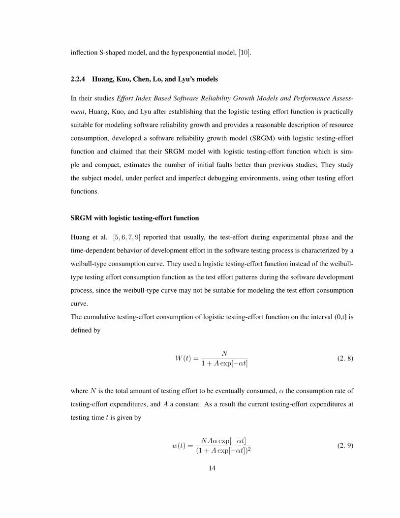
In their studies Effort Index Based Software Reliability Growth Models and Performance Assess-

ment, Huang, Kuo, and Lyu after establishing that the logistic testing effort function is practically

suitable for modeling software reliability growth and provides a reasonable description of resource

consumption, developed a software reliability growth model (SRGM) with logistic testing-effort

function and claimed that their SRGM model with logistic testing-effort function which is sim-

ple and compact, estimates the number of initial faults better than previous studies; They study

the subject model, under perfect and imperfect debugging environments, using other testing effort

functions.

SRGM with logistic testing-effort function

Huang et al. [5, 6, 7, 9] reported that usually, the test-effort during experimental phase and the

time-dependent behavior of development effort in the software testing process is characterized by a

weibull-type consumption curve. They used a logistic testing-effort function instead of the weibull-

type testing effort consumption function as the test effort patterns during the software development

process, since the weibull-type curve may not be suitable for modeling the test effort consumption

curve.

The cumulative testing-effort consumption of logistic testing-effort function on the interval (0,t] is

defined by

W (t) =N

1 + A exp[−αt](2. 8)

where N is the total amount of testing effort to be eventually consumed, α the consumption rate of

testing-effort expenditures, and A a constant. As a result the current testing-effort expenditures at

testing time t is given by

w(t) =NAα exp[−αt]

(1 + A exp[−αt])2(2. 9)

14

where w(t) is a smooth bell-shaped function with a left-tailed side, and reaches it maximum value

at time

tmax =lnA

α(2. 10)

This SRGM model is based on the following assumtions:

(i) The fault removal process follows the Non-Homogeneous Poisson Process (NHPP )

(ii) The software system is subject to failures at random times caused by faults remaining in the

system.

(iii) The mean number of faults detected in the time interval (t, t+ dt]by the current test-effort is

proportional to the mean number of remaining faults in the system.

(iV) The proportionality is constant over time.

(V) The consumption curve of testing effort is modeled by a logistic testing-effort function.

(Vi) Each time a failure occurs, the fault that caused it is immediately removed, and no new faults

are introduced.

Thus, the differential equation is given by

dm(t)dt

= w(t)r[a−m(t)], a > 0, 0 < r < 1 (2. 11)

describes analytically the testing-based-effort.

The solution of the above differential equation, under the boundary condition

m(0) = 0 is

m(t) = a(1− e−r(W (t)−W (0))) (2. 12)

where m(t) is the expected number of faults detected on the interval (0, t], w(t) the current testing-

effort consumption at time t, a the expected number of initial faults, and r the error detection rate

per unit testing-effort at testing time t that satisfies r > 0.

15

Yamada S-shaped model with logistic testing-effort function

Huang et al. reported, [5], that the Delayed S-shaped SRGM model proposed by Yamada et al. was

a simple modification of the NHPP to get an S-shaped growth curve for the cumulative number of

failures detected. Since the testing phase contains a fault detection process and a fault isolation pro-

cess, Huang et al. developed the following relationship between m(t) and w(t) to extend Yamada’s

S-shaped software reliability model: [5]

df(t)dt

1w(t)

= ω[a− f(t)] (2. 13)

and

dg(t)dt

1w(t)

= ε[f(t)− g(t)] (2. 14)

where f(t) is the cumulative number of failures detected up to time t and g(t) the cumulative num-

ber of failures isolated up to time t. Under boundary conditions f(0) = g(0) = 0 the solutions of

the above differential equations are respectively,

f(t) = a(1− e−ω(W (t)−W (0))) = a(1− e−ωW ∗(t)) (2. 15)

and

g(t) = a[1− 1ω − ε

(ωe−εW ∗(t) − εe−ωW ∗(t)

)] (2. 16)

where ω and ε are the failure detection rate and the failure isolation rate, respectively.

Assuming fault detection rate parameter ω ∼= ε, the NHPP model with a Delayed S-shaped growth

curve of detected software faults is given by

m(t) = a(1− (1 + Ψ(W (t)−W (0))e−Ψ(W (t)−W (0))) = a(1− (1 + ΨW ∗(t)e−ΨW ∗(t)) (2. 17)

16

where Ψ is the fault detection rate per unit testing-effort at testing time t satisfying Ψ > 0.

2.3 Development of The proposed Model

The objective of this section is to develop a software reliability growth model that

(i) does not assume any prior distribution

(ii) is free of convergence assumption

(iii) is simple

(iV) fits very well the cumulative number of software faults found and corrected

(V) estimates the remaining number of software faults in the software package

(Vi) yields accurate parameter estimates

Thus, allowing software developers to predict or decide when a software is ready to be released.

Our proposed model which is not subject to errors generated by discretization, provides accurate

parameter estimates when sufficient data points are available.

2.3.1 The Logistic Regression Model

The proposed logistic model is suitable for software reliability assessment. While in linear regres-

sion models the outcome variable is assumed to be continuous, in logistic regression models the

outcome variable is binary or dichotomous. It is often the case that the outcome variable is discrete.

In any regression problem, the key quantity when it exists is the conditional mean,

E(y|x) = β0+β1x, where y denotes the outcome variable and x denotes a value of the independent

variable, which can take on any value, [4]. With dichotomous data the conditional mean must be

greater than or equal to zero and less than or equal to one, 0 ≤ [E(y|x)] ≤ 1. The change in E(y|x)

per-unit change in x becomes progressively smaller as the conditional mean gets closer to zero or

one, and then, the curve is said to be S-shaped. When the logistic distribution is used, the logistic

regression model we use is

E(y|x) = π(x) =eβ0+β1x

1 + eβ0+β1x

with a dichotomous outcome variable y = π(x) + ε, the quantity ε is called the error that expresses

an observation’s deviation from the conditional mean [4]. In logistic regression the quantity ε may

assume one of two possible values. If y = 1 then ε = 1− π(x) with probability π(x), and if y = 0

17

then ε = −π(x) with probability 1− π(x). Thus, ε has a distribution with mean zero and variance

equal to π(x)[1 − π(x)]. That is, the conditional distribution of the outcome variable follows a

binomial distribution with probability given by the conditional mean, π(x), [4].

In Summary, in regression analysis when the outcome variable is dichotomous, [4], we have

i) The conditional mean of the regression equation must be formulated to be bounded between zero

and one. The above logistic regression model π(x) satisfies this constraint.

ii) The binomial, not the normal, distribution describes the distribution of the errors and will be the

statistical distribution upon which the analysis is based.

These characterizing properties of the logistic model makes it useful as a growth curve model.

2.3.2 Model Description

Let L(t) be the cumulative amount of software faults found and corrected in the debugging phase

during exposure time interval [0,t]. The parameter k (k > 0) represents the initial total number of

software faults in the software prior to the debugging phase as in [1].

The logistic curve model is described by the differential equation

dL(t)dt

=α

kL(t)(k − L(t)), t ≥ 0 (2. 18)

where α (α > 0) and k (k > 0) are constant parameters to be estimated by regression analysis [1].

Let

P (t) =L(t)k

Then, from Equation 4. 8, we have

dP (t)dt

= αP (t)(1− P (t)), t ≥ 0, P (0) =1

1 + m, m À k

where

P (t) =L(t)k

is the cumulative fraction number of software failures found and corrected in the debugging phase

during exposure time interval [0,t].

18

The solution of the above differential equation is

P (t) =1

1 + me−αt(2. 19)

where m is the constant of integration. Note that the graph of P (t) is S-shaped and 0 ≤ P (t) ≤ 1.

A software fault found and corrected at each instant is a binary outcome variable. We assume that

the binomial distribution describes the distribution of the errors and will be the statistical distribution

upon which the analysis is based, [4].

Fewer software faults are found early in the testing and long into the testing and debugging phase

when most of the faults are found and corrected and only a few faults are left in the software. For

such cases we propose a Logistic Like Model to estimate the parameters k, m and α of P (t).

2.3.3 Parameters Estimation

Our proposed model depends on an accurate estimate of the total number of faults k in a given soft-

ware. Let ti be the random detection time of the ith software fault . Let N denote the total number

of available software faults found and corrected up to time tN . We assume that once a software fault

is found it is corrected for good. Using the N available data points collected during the testing and

debugging phase and increasing N by 1 after each sequential logistic regression run, we run a series

of logistic regressions models of the form

P (t) =eβ0+β1t

1 + eβ0+β1t

where β0 and β1 are the parameters of the logistic regression model, to estimate the true cumulative

percentage number of software faults found and corrected in a given software up to time t of its

testing and debugging process

P (t) =L(t)k

=1

1 + me−αt

That is, starting with the N available data value, and assuming that all the software faults were

found during the testing and debugging phase, we run a logistic regression to obtain an estimate

P (t)N =eβ0N+β1N t

1 + eβ0N+β1N t

19

of

P (t)N =L(t)k

=1

1 + me−αt

Now, using

L(t)N = (N)(P (t)N ) =Neβ0N+β1N t

1 + eβ0N+β1N t

where β0N and β1N are the Maximum Likelihood Estimators of the parameters β0 and β1, we

obtain the predicted cumulative number of software failure assuming that there were N faults in the

software which estimates the true cumulative number of software faults L(t) in the given software.

Now evaluating

L(t)N = (N)(P (t)N ) =Neβ0N+β1N t

1 + eβ0N+β1N t

at each ti, i = 1, 2, ..., N , the predicted cumulative failure behavior is obtained, for this run, assum-

ing that there were N faults in the software. Finally, we can estimate the true mean square error

MSEN of the actual and predicted cumulative number of software faults by calculating

MSEN =∑N

i=1(L(ti)N − L(ti))2

N

What if there is one more fault remaining in the software? For our second run, assuming that

there are N + 1 software faults in the software of which N are found and corrected, we repeat the

above procedure to obtain an estimate

P (t)N+1 =eβ0N+1+β1N+1t

1 + eβ0N+1+β1N+1t

of

P (t)N+1 =L(t)k

=1

1 + me−αt

and

L(t)N+1 = (N + 1)(P (t)N+1) =(N + 1)eβ0N+1+β1N+1t

1 + eβ0N+1+β1N+1t

where β0N+1 and β1N+1 are the Maximum Likelihood Estimators of the parameters β0 and β1

evaluating

L(t)N+1 = (N + 1)(P (t)N+1) =(N + 1)eβ0N+1+β1N+1t

1 + eβ0N+1+β1N+1t

20

at each ti, i = 1, 2, ..., N , the predicted cumulative failure behavior is obtained, for the second run,

assuming that there were N + 1 faults in the software. Then, we can estimate the true mean square

error MSEN+1 of the actual and predicted cumulative number of software faults by calculating

MSEN+1 =∑N

i=1(L(ti)N+1 − L(ti))2

N

We then plot the estimated MSEi as i takes the values i = N, N + 1, N + 2, ....

Now, we propose on using an estimate of k, k where the minimum MSEi occurs, that is, k = im,

where im is one of the positive integers N, N + 1, N + 2, ... at which MSEi is minimal.

Having an estimate of k, k = im, we set up our best fit logistic like regression model in the

minimal mean square error sense.

proposing

P (t) =eβ0im

+β1imt

1 + eβ0im+β1im

t

to estimate the true cumulative percentage number of software failures found and corrected during

debugging and testing phase up to testing and debugging time t, we obtain estimates of m and α

needed in Equation 4. 9 as follows:

By identification method we obtain

11 + me−αt

≡ eβ0im+β1im

t

1 + eβ0im+β1im

t=

11 + 1

eβ0im e

β1imt

=1

1 + e−β0im e−β1imt

(2. 20)

Now comparing the first and the last term of Equation 2. 20, we obtain the following estimates of

m and α:

m = e−β0im

α = β1im

where β0im and β1im are the Maximum Likelihood Estimators of the parameters β0 and β1, using

k = im and im the positive integer from N,N + 1, N + 2, ... at which MSEi is minimal.

Thus, an estimate of P (t) can be obtained using

P (t) =1

1 + me−bαt=

1


21

Note that, since β0im < 0 and β1im > 0, we obtain −β0im > 0 and −β1im < 0. As a result,

P (t) satisfies the conditions of a distribution function.

Finally the cumulative failure behavior of the proposed model for a given software is given by

L(t) =k

1 + me−bαt=

im


It will be shown that our proposed estimate of L(t) gives good results in comparison to the other

models that are commonly used.

2.4 Comparisons of Models: Numerical Application to Software Failure Data

In this section we shall compare, using the mean square error, several frequently and pre-existing

models to our Logistic model on seven sets of actual software failure data obtained from actual

projects. It will be shown to that our proposed model provides not only competitive parameters

estimates and also gives a very good modeling of the S-shaped cumulative number of software

faults found and corrected curves during testing and debugging phase. The Kolmogorov-Smirnov

test will be also used to assess the goodness-of-fit of our predicted versus the actual data.

2.4.1 PL/I software Failure Data

For application to actual software reliability failures data, and comparison of our proposed model

with the previous models, we analyze a data set, PL/I application program test data given by

Table 1, on page 23, reported and studied previously by Ohba [10] in 1984, and later analyzed by

Huang, Kuo, and Lyu in 1997 and 2001 in their research [5, 6, 7, 9, 24]. Huang and al. reported that

for the PL/I database application program, the size of the software is approximately 1,317,000 line

of codes, the time axis is the execution time ,and that the cumulative number of faults found and

detected after a long testing period was 358, value to be used as an addition comparison criterion,

[7].

22

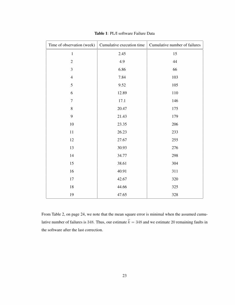
Table 1: PL/I software Failure Data

Time of observation (week) Cumulative execution time Cumulative number of failures

1 2.45 15

2 4.9 44

3 6.86 66

4 7.84 103

5 9.52 105

6 12.89 110

7 17.1 146

8 20.47 175

9 21.43 179

10 23.35 206

11 26.23 233

12 27.67 255

13 30.93 276

14 34.77 298

15 38.61 304

16 40.91 311

17 42.67 320

18 44.66 325

19 47.65 328

From Table 2, on page 24, we note that the mean square error is minimal when the assumed cumu-

lative number of failures is 348. Thus, our estimate k = 348 and we estimate 20 remaining faults in

the software after the last correction.

23

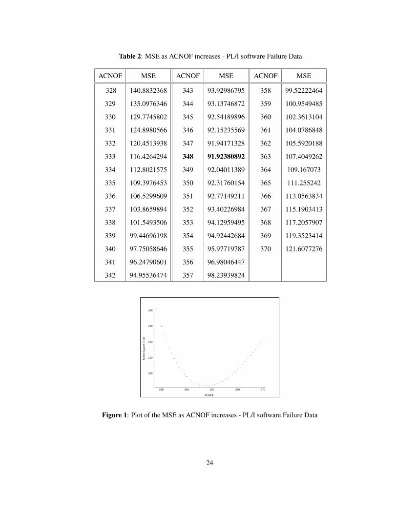
Table 2: MSE as ACNOF increases - PL/I software Failure Data

ACNOF MSE ACNOF MSE ACNOF MSE

328 140.8832368 343 93.92986795 358 99.52222464

329 135.0976346 344 93.13746872 359 100.9549485

330 129.7745802 345 92.54189896 360 102.3613104

331 124.8980566 346 92.15235569 361 104.0786848

332 120.4513938 347 91.94171328 362 105.5920188

333 116.4264294 348 91.92380892 363 107.4049262

334 112.8021575 349 92.04011389 364 109.167073

335 109.3976453 350 92.31760154 365 111.255242

336 106.5299609 351 92.77149211 366 113.0563834

337 103.8659894 352 93.40226984 367 115.1903413

338 101.5493506 353 94.12959495 368 117.2057907

339 99.44696198 354 94.92442684 369 119.3523414

340 97.75058646 355 95.97719787 370 121.6077276

341 96.24790601 356 96.98046447

342 94.95536474 357 98.23939824

100

110

120

130

140

Mea

n S

quar

e E

rror

330 340 350 360 370

ACNOF

Figure 1: Plot of the MSE as ACNOF increases - PL/I software Failure Data

24

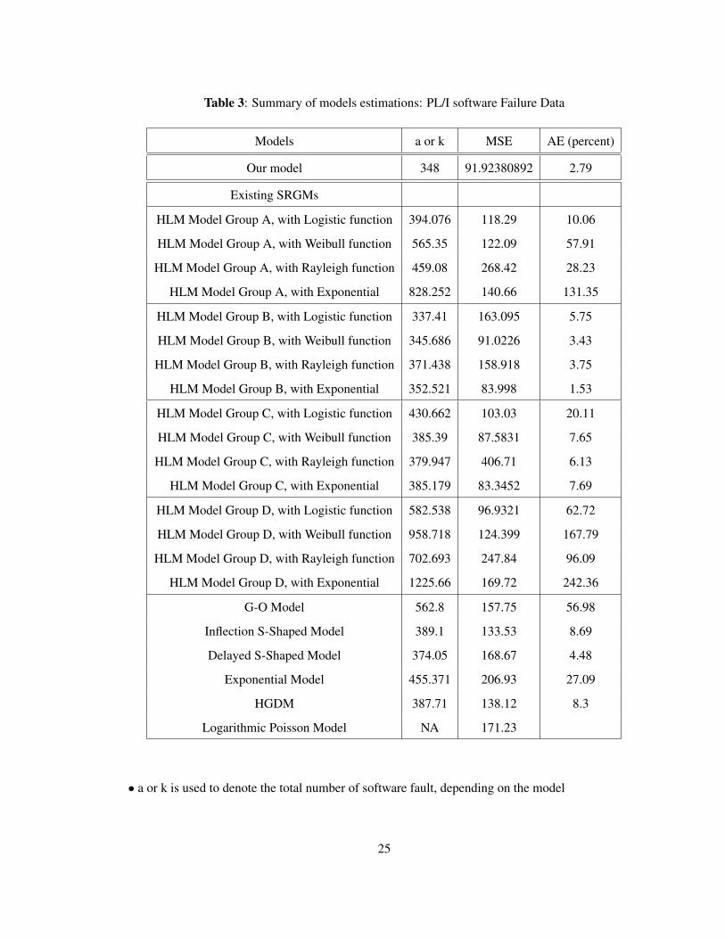
Table 3: Summary of models estimations: PL/I software Failure Data

Models a or k MSE AE (percent)

Our model 348 91.92380892 2.79

Existing SRGMs

HLM Model Group A, with Logistic function 394.076 118.29 10.06

HLM Model Group A, with Weibull function 565.35 122.09 57.91

HLM Model Group A, with Rayleigh function 459.08 268.42 28.23

HLM Model Group A, with Exponential 828.252 140.66 131.35

HLM Model Group B, with Logistic function 337.41 163.095 5.75

HLM Model Group B, with Weibull function 345.686 91.0226 3.43

HLM Model Group B, with Rayleigh function 371.438 158.918 3.75

HLM Model Group B, with Exponential 352.521 83.998 1.53

HLM Model Group C, with Logistic function 430.662 103.03 20.11

HLM Model Group C, with Weibull function 385.39 87.5831 7.65

HLM Model Group C, with Rayleigh function 379.947 406.71 6.13

HLM Model Group C, with Exponential 385.179 83.3452 7.69

HLM Model Group D, with Logistic function 582.538 96.9321 62.72

HLM Model Group D, with Weibull function 958.718 124.399 167.79

HLM Model Group D, with Rayleigh function 702.693 247.84 96.09

HLM Model Group D, with Exponential 1225.66 169.72 242.36

G-O Model 562.8 157.75 56.98

Inflection S-Shaped Model 389.1 133.53 8.69

Delayed S-Shaped Model 374.05 168.67 4.48

Exponential Model 455.371 206.93 27.09

HGDM 387.71 138.12 8.3

Logarithmic Poisson Model NA 171.23

• a or k is used to denote the total number of software fault, depending on the model

25

Table 3, on page 25, provides a comparative summary of our estimate k along with several other

estimates from some pre-existing models and the mean square error for each model. Table 3 also

shows that by predicting 348 faults associated with a mean square error of 91.92380892 our pro-

posed model, LR-Model, without any major assumptions, fitting well trough the K-S goodness-of-fit

(D = 0.1053, P = 1.00), demonstrates better performance than most of the pre-existing models.

50

100

150

200

250

300

Num

ber

of F

aults

0 5 10 15 20

Debugging Week

Figure 2: Comparison Of the PL/I Software Failure Data and our Predicted

Figure 2 shows that our LR-Model’s estimated cumulative number of software faults found and

corrected fits very well the actual cumulative software failure data.

2.4.2 Tohma’s Software Failure Data

To evaluate and compare our proposed model with the others, we use a data set, the pattern of

discovery of errors Table 4, on page 27, reported and studied by Tohma [11] in 1989, and later

analyzed by Huang, Kuo, and Lyu in 2001, in their studies [5, 9]. Thoma, in his paper Hyper-

Geometric Distribution Model to Estimate the number of Residual Software Faults, reported that

for pattern of discovery of errors program, in Table 4, debug times instead of the number of test

workers, the number of detected faults and the cumulated detected faults were recorded day by day.

26

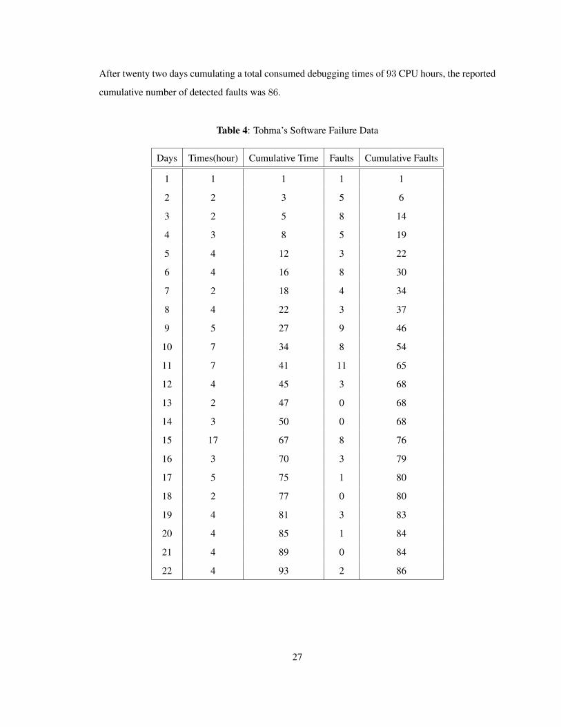
After twenty two days cumulating a total consumed debugging times of 93 CPU hours, the reported

cumulative number of detected faults was 86.

Table 4: Tohma’s Software Failure Data

Days Times(hour) Cumulative Time Faults Cumulative Faults

1 1 1 1 1

2 2 3 5 6

3 2 5 8 14

4 3 8 5 19

5 4 12 3 22

6 4 16 8 30

7 2 18 4 34

8 4 22 3 37

9 5 27 9 46

10 7 34 8 54

11 7 41 11 65

12 4 45 3 68

13 2 47 0 68

14 3 50 0 68

15 17 67 8 76

16 3 70 3 79

17 5 75 1 80

18 2 77 0 80

19 4 81 3 83

20 4 85 1 84

21 4 89 0 84

22 4 93 2 86

27

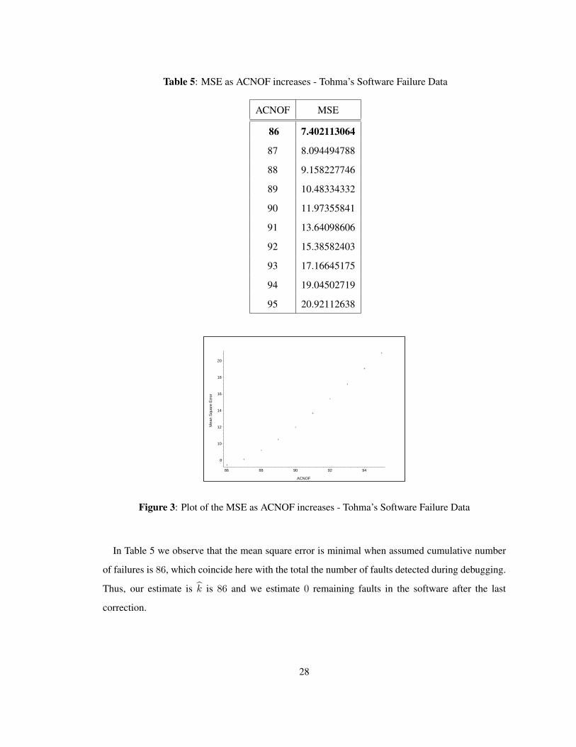
Table 5: MSE as ACNOF increases - Tohma’s Software Failure Data

ACNOF MSE

86 7.402113064

87 8.094494788

88 9.158227746

89 10.48334332

90 11.97355841

91 13.64098606

92 15.38582403

93 17.16645175

94 19.04502719

95 20.92112638

8

10

12

14

16

18

20

Mea

n S

quar

e E

rror

86 88 90 92 94

ACNOF

Figure 3: Plot of the MSE as ACNOF increases - Tohma’s Software Failure Data

In Table 5 we observe that the mean square error is minimal when assumed cumulative number

of failures is 86, which coincide here with the total the number of faults detected during debugging.

Thus, our estimate is k is 86 and we estimate 0 remaining faults in the software after the last

correction.

28

Table 6: Summary of models estimations: Tohma’s Software Failure Data

Models a or k MSE

Our model 86 7.40211306

Existing SRGMs

HLM Model Group A, with Logistic function 88.8931 25.2279

HLM Model Group A, with Weibull function 87.0318 7.772

HLM Model Group A, with Rayleigh function 86.1616 3.91643

HLM Model Group B, with Logistic function 89.4528 14.06603

HLM Model Group B, with Weibull function 87.3126 18.956772

HLM Model Group B, with Rayleigh function 87.3472 20.4568

HLM Model Group C, with Logistic function 97.5332 7.354363

HLM Model Group C, with Weibull function 97.6841 6.5909

HLM Model Group C,with Rayleigh function 112.182 6.60318

HLM Model Group D, with Logistic function 106.1 7.33727

HLM Model Group D, with Weibull function 114.52 6.36531

HLM Model Group D, with Rayleigh function 112.183 6.60318

G-O Model 137.072 25.33

Delayed S-Shaped Model 88.6533 6.31268

HGDM 88.6533 6.31268

S-Y Models 73.11837775 196.7452124

• a or k is used to denote the total number of software fault, depending on the model

Table 6 provides a comparative summary of our estimate K along with several other estimates

from some pre-existing models and the mean square error for each model. Table 6 also shows that

by predicting 86 faults associated with a mean square error of 7.40211306 our proposed model,

LR-Model, without any major assumptions, fitting well trough the K-S goodness-of-fit

(D = 0.090, P = 1.00), demonstrates better performance than most of the other models.

29

0

20

40

60

80

Num

ber

of F

aults

5 10 15 20 25

Debugging Day

Figure 4: Comparison of Tohma’s Software Failure Data and our Predicted

Figure 4 shows that our LR-Model’s predictive cumulative number of software faults found and

corrected fits very well the actual cumulative software failure data. Thus, our proposed model

which is easier to use and free of any major assumption gives very good if not better results then

other models used in industry.

2.4.3 The F 11-D program test data

Here, we shall compare our model effectiveness with other commonly used models in the subject

area. We analyze a set of software reliability field data of a data reduction program called the

F 11-D program, in Table 7, on page 31, reported to be presented by Moranda 1975 and studied by

Forman and Singpurwalla [13] in 1977 in their paper An Empirical Stopping Rule for Debugging

and Testing Computer Software, later studied by Dale and Harris in 1982, in their paper Approaches

to software reliability prediction [14], and by Tohma in 1989, [11]. The F 11-D program is reported

to consist of approximately 3 − 4 thousand Fortran statements [13]. As recorded in Table 7 after

debugging the program for a total of 226.11 seconds of CPU time, a total of 107 software errors

were detected.

30

Table 7: The F 11-D program test data

I.N. Date N.E.D.I.N C.N.E, N M.L.E of N

1 1/12 8 8 9

2 1/15 7 15 16

3 1/16 1 16 17

4 1/17 8 24 24

5 1/18 16 40 43

6 1/19 18 58 60

7 1/22 13 71 73

8 1/23 8 79 81

9 1/24 9 88 90

10 1/25 2 90 92

11 1/26 6 96 99

12 1/27 3 99 100

13 1/29 3 102 102

14 1/30 2 104 104

15 1/31 3 107 107

• I.N.: Interval Number • N.E.D.I.N.: Number of errors detected in Interval

Table 8: MSE as ACNOF increases - The F 11-D program test data

ACNOF MSE

107 9.009282277

108 10.74342705

109 12.77994731

110 14.98197705

111 17.37213712

31

10

12

14

16

Mea

n S

quar

e E

rror

107 108 109 110 111

ACNOF

Figure 5: Plot of the MSE as ACNOF increases - The F 11-D program test data

Table 8, on page 31, shows that the mean square error is minimal when assumed cumulative

number of failures is to 107 which agrees with the total the number of faults detected during actual

debugging. Thus, our estimate k = 107 and we estimate 0 remaining faults in the software after the

last modification.

Table 9: Summary of models estimations: The F 11-D program test data

Models k or N MSE

Our model 107 9.009282277

Existing SRGMs

F-S Model 107 2.8

S-Y Models 107.4860452 8.955939003

Table 9 provides a comparative summary of our estimate k along with a few other estimates from

some pre-existing models and the mean square error for each model. Table 9 also shows that by

predicting 107 faults associated with a mean square error of 9.009282277 our proposed model, LR-

Model, fitting well trough the K-S goodness-of-fit (D = 0.0667, P = 1.00), demonstrates a very

good fit.

Our LR-Model, although does not demonstrates better performance than most of the pre-existing

models in the mean square error sense, confirms Forman and Singpurwalla’s empirical stopping rule

32

for debugging and testing Computer Software for this software package. Forman and Singpurwalla,

[13], considering a simple model for describing the failures of computer software, outlined some

difficulties associated with the application of the method of maximum likelihood for estimating the

number of errors in a code. As pointed out in their conclusions, [13], their estimation procedure

leading them to a stopping rule for debugging the software, calls for a critical examination of the

actual likelihood function at each stage of the procedure. Forman and Singpurwalla, after demon-

strating the usefulness of their technique on the the F 11-D program software reliability failure data,

advise the software testing and debugging team to stop testing after 107 software faults were found

and corrected [13]. Forman and Singpurwalla have also reported in [13] that since their technique

is empirical in nature, a certain amount of subjectivity in executing it is inherently present. Dale

reported that the maximum likelihood estimator can be highly misleading, and criticized Forman

and Singpurwalla’s maximum likelihood estimation of the remaining number of software faults:

”the estimated number of bugs remaining at the end of the twelfth debugging interval is the same as

at the end of the third interval, despite the fact that 83 bugs have been corrected in the meantime”,

[14].

20

40

60

80

100

Num

ber

of F

aults

0 2 4 6 8 10 12 14 16 18 20

Debugging Interval

Figure 6: Comparison of The F 11-D program test data and our Predicted

33

The Figure 6, on page 33, shows that our LR-Model’s predictive cumulative number of software

faults found and corrected fits very well the actual cumulative software failure data. Thus, our

proposed model which is easier to use and free of any major assumption gives very good if not

better results then other models used in industry.

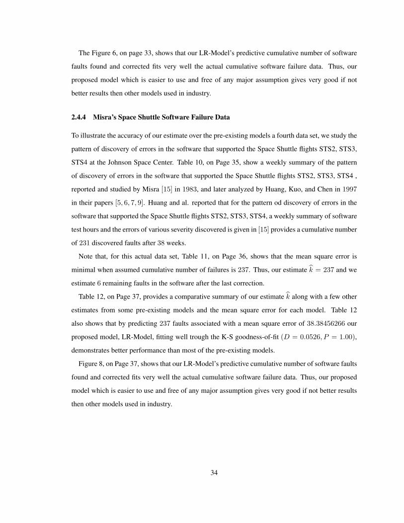
2.4.4 Misra’s Space Shuttle Software Failure Data

To illustrate the accuracy of our estimate over the pre-existing models a fourth data set, we study the

pattern of discovery of errors in the software that supported the Space Shuttle flights STS2, STS3,

STS4 at the Johnson Space Center. Table 10, on Page 35, show a weekly summary of the pattern

of discovery of errors in the software that supported the Space Shuttle flights STS2, STS3, STS4 ,

reported and studied by Misra [15] in 1983, and later analyzed by Huang, Kuo, and Chen in 1997

in their papers [5, 6, 7, 9]. Huang and al. reported that for the pattern od discovery of errors in the

software that supported the Space Shuttle flights STS2, STS3, STS4, a weekly summary of software

test hours and the errors of various severity discovered is given in [15] provides a cumulative number

of 231 discovered faults after 38 weeks.

Note that, for this actual data set, Table 11, on Page 36, shows that the mean square error is

minimal when assumed cumulative number of failures is 237. Thus, our estimate k = 237 and we

estimate 6 remaining faults in the software after the last correction.

Table 12, on Page 37, provides a comparative summary of our estimate k along with a few other

estimates from some pre-existing models and the mean square error for each model. Table 12

also shows that by predicting 237 faults associated with a mean square error of 38.38456266 our

proposed model, LR-Model, fitting well trough the K-S goodness-of-fit (D = 0.0526, P = 1.00),

demonstrates better performance than most of the pre-existing models.

Figure 8, on Page 37, shows that our LR-Model’s predictive cumulative number of software faults

found and corrected fits very well the actual cumulative software failure data. Thus, our proposed

model which is easier to use and free of any major assumption gives very good if not better results

then other models used in industry.

34

Table 10: Misra’s Space Shuttle Software Failure Data

Week Cr.E Ma.E Mi.E C.E Week Cr.E Ma.E Mi.E C.E

1 0 6 9 15 20 0 2 3 136

2 0 2 4 21 21 0 1 1 138

3 0 1 7 29 22 0 3 2 143

4 1 1 6 37 23 0 2 4 149

5 0 3 5 45 24 0 4 5 158

6 0 1 3 49 25 0 1 0 159

7 0 2 2 53 26 0 2 2 163

8 0 3 5 61 27 0 2 0 165

9 0 2 4 67 28 0 2 2 169

10 0 0 2 69 29 0 1 3 173

11 0 3 4 76 30 1 2 6 182

12 0 1 7 84 31 1 2 3 188

13 0 3 0 87 32 0 0 1 189

14 0 0 5 92 33 0 2 1 192

15 0 2 3 97 34 0 2 4 198

16 0 5 3 105 35 0 3 3 204

17 0 5 3 113 36 0 1 2 207

18 0 2 4 119 37 1 2 11 221

19 0 2 10 131 38 0 1 9 231

• Cr.E: Critical Errors

• Ma.E: Major Errors

• Mi.E: Minor Errors

• C.E.: Cumulative Errors.

35

Table 11: MSE as ACNOF increases - Misra’s Space Shuttle Software Failure Data

ACNOF MSE

231 39.24889498

232 38.96808896

233 38.73239432

234 38.55970054

235 38.4544495

236 38.39724536

237 38.38456266

238 38.4183368

239 38.49035903

240 38.6077261

241 38.75830898

242 38.94298088

243 39.16746369

38.4

38.6

38.8

39

39.2

Mea

n S

quar

e E

rror

232 234 236 238 240 242

ACNOF

Figure 7: MSE as ACNOF increases - Misra’s Space Shuttle Software Failure Data

36

Table 12: Summary of models estimations: Misra’s Space Shuttle Software Failure Data

Models a or K MSE

Our model 237 38.38456266

G-O Model 597.887 78.87

S-Y Models 200.8486903 265.3335203

50

100

150

200

Num

ber

of F

aults

0 10 20 30 40 50

Debugging Week

Figure 8: Comparison of Misra’s Space Shuttle Software Failure Data and our Predicted

37

2.4.5 Musa’s System T1 software Failure Data

To assess and compare our proposed model with the others pre-existing models, we study the System

T1 of the Rome Air Development Center (RADC) projects Table 13, reported by Musa, [53], and

later studied by Huang, Kuo, and Chen in 1997 in their papers [6, 7, 9]. The system T1 is reported to

be used for a real-time command and control application; the size of the software is approximately

21, 700 object instructions. To complete the test, it took twenty-one weeks, nine programmers,

about 25.3 CPU hours to remove 136 software errors.

Table 13: System T1

Interval of observation (interval length = 5 Days) Cumulative number of failures

1 3

2 4

3 6

4 16

5 16

6 22

7 29

8 29

9 31

10 42

11 48

12 63

13 78

14 92

15 105

16 122

17 132

18 135

19 136

38

Table 14: MSE as ACNOF increases - System T1

ACNOF MSE ACNOF MSE

136 59.73849038 164 20.74581198

137 56.45913482 165 20.43461528

138 53.51272497 166 20.16955946

139 50.74510692 167 19.93233847

140 48.05754858 168 19.73619002

141 45.68399539 169 19.56559153

142 43.41103347 170 19.42895933

143 41.32847537 171 19.3171211

144 39.34891981 172 19.2292499

145 37.56874349 173 19.16859798

146 35.97196455 174 19.1305098

147 34.38348791 175 19.11480503

148 32.98043088 176 19.11803102

149 31.58854155 177 19.14235957

150 30.37887505 178 19.18716939

151 29.25654819 179 19.24351235

152 28.22982752 180 19.31848929

153 27.28001268 181 19.41178997

154 26.36265956 182 19.52408042

155 25.52487927 183 19.63968954

156 24.77120468 184 19.77192253

157 24.09448225 185 19.91998986

158 23.44652547 186 20.08486024

159 22.90736243 187 20.24602725

160 22.35927548 188 20.4212037

161 21.90723966 189 20.61078576

162 21.45572338 190 20.81366771

163 21.0866153

39

20

30

40

50

60

Mea

n S

quar

e E

rror

140 150 160 170 180 190

ACNOF

Figure 9: Plot of the MSE as ACNOF increases - System T1

Table 14, on page 39, shows that the Mean Square Error is minimal when assumed cumulative

number of failures is to 175. Thus, our estimate k = 175 and we estimate 39 remaining faults in the

software after the last correct.

Table 15, on page 41, provides a comparative summary of our estimate k along with a few other

estimates from some pre-existing models and the mean square error for each model. Table 15

also shows that by predicting 175 faults associated with a mean square error of 19.11480503 our

proposed model, LR-Model, fitting well trough the K-S goodness-of-fit (D = 0.1053, P = 1.00),

demonstrates better performance than most of the pre-existing models.

40

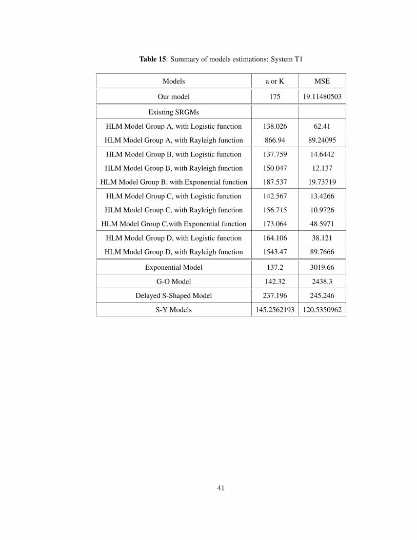
Table 15: Summary of models estimations: System T1

Models a or K MSE

Our model 175 19.11480503

Existing SRGMs

HLM Model Group A, with Logistic function 138.026 62.41

HLM Model Group A, with Rayleigh function 866.94 89.24095

HLM Model Group B, with Logistic function 137.759 14.6442

HLM Model Group B, with Rayleigh function 150.047 12.137

HLM Model Group B, with Exponential function 187.537 19.73719

HLM Model Group C, with Logistic function 142.567 13.4266

HLM Model Group C, with Rayleigh function 156.715 10.9726

HLM Model Group C,with Exponential function 173.064 48.5971

HLM Model Group D, with Logistic function 164.106 38.121

HLM Model Group D, with Rayleigh function 1543.47 89.7666

Exponential Model 137.2 3019.66

G-O Model 142.32 2438.3

Delayed S-Shaped Model 237.196 245.246

S-Y Models 145.2562193 120.5350962

41

The Figure 10 below, shows that our LR-Model’s predictive cumulative number of software faults

found and corrected fits very well the actual cumulative software failure data. Thus, our proposed

model which is easier to use and free of any major assumption gives very good if not better results

then other models used in industry.

0

20

40

60

80

100

120

140

160

Num

ber

of F

aults

5 10 15 20 25 30

Debugging Interval

Figure 10: Comparison of the System T1 data set and our Predicted

2.4.6 Ohba’s On-line data entry software test Data

For application to actual software reliability failures data,and comparison of our proposed model

with the previous models, we analyze the sixth data set, Ohba’s On-line data entry software package

test data Table 16, on page 43, reported by Ohba in 1984 [10] and later analyzed by Tohma, Jacoby,

Murata, and Yamamoto in 1989 in their papers [11]. The small on-line data entry control software

package reported to have been available since 1980 in Japan, has an approximate size of 40000

lines of code; the testing time was measured on the basis of the number of shifts spent running test

cases and analyzing the results. the number of persons on the test team was reported to be constant

throughout the test period; During the twenty-one days of test, 46 software errors were removed

[10]; the cumulative number of faults found and detected after a long testing period (three years)

was reported to be 69, value to be used as an addition comparison criterion.

42

Table 16: Ohba’s On-line data entry software test Data

Time of observation (day) Cumulative number of faults

1 2

2 3

3 4

4 5

6 9

7 11

8 12

9 19

10 21

11 22

12 24

13 26

14 30

15 31

16 37

17 38

18 41

19 42

20 45

21 46

43

Table 17: MSE as ACNOF increases - Ohba’s On-line data entry software test Data

ACNOF MSE

46 2.877909807

47 2.439920792

48 2.139457102

49 1.945403281

50 1.832603369

51 1.784785998

52 1.786831674

53 1.828631846

54 1.900772326

55 1.998562288

56 2.115459903

57 2.24590523

58 2.387993439

59 2.541360386

60 2.699959644

1.8

2

2.2

2.4

2.6

2.8

Mea

n S

quar

e E

rror

46 48 50 52 54 56 58 60

ACNOF

Figure 11: Plot of the MSE as ACNOF increases - Ohba’s On-line data entry software test Data

44

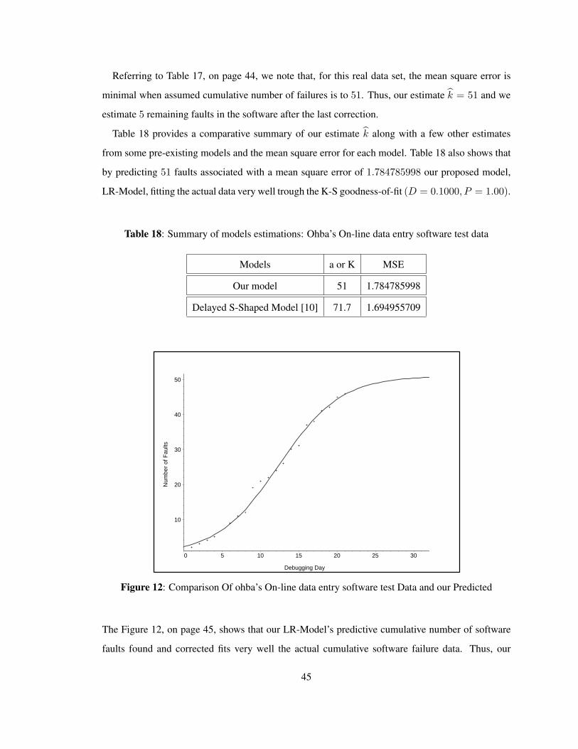
Referring to Table 17, on page 44, we note that, for this real data set, the mean square error is

minimal when assumed cumulative number of failures is to 51. Thus, our estimate k = 51 and we

estimate 5 remaining faults in the software after the last correction.

Table 18 provides a comparative summary of our estimate k along with a few other estimates

from some pre-existing models and the mean square error for each model. Table 18 also shows that

by predicting 51 faults associated with a mean square error of 1.784785998 our proposed model,

LR-Model, fitting the actual data very well trough the K-S goodness-of-fit (D = 0.1000, P = 1.00).

Table 18: Summary of models estimations: Ohba’s On-line data entry software test data

Models a or K MSE

Our model 51 1.784785998

Delayed S-Shaped Model [10] 71.7 1.694955709

10

20

30

40

50

Num

ber

of F

aults

0 5 10 15 20 25 30

Debugging Day

Figure 12: Comparison Of ohba’s On-line data entry software test Data and our Predicted

The Figure 12, on page 45, shows that our LR-Model’s predictive cumulative number of software

faults found and corrected fits very well the actual cumulative software failure data. Thus, our

45



2.4.7 Tohma’s software package test Data


with the previous models, we analyze a last data set, the field report of the test of a software for

monitoring and real-time control Table 19, on page 47, reported by Tohma, Tohunaga, and Nagase

in 1989 [11, 16, 18] and later analyzed by Doli, Wakana, Osaki, and Trivedi in there study, [17].

The software is reported to consist of about 200 modules, each of which is about 1000 lines in a

high-level language like Fortran.

From Table 20, on page 48, we note that for this real data set, the mean square error is minimal

when assumed cumulative number of failures is to 481. Thus, our estimate k = 481 and we estimate

0 remaining faults in this software package after the last correction.

Table 21, on page 49, provides a comparative summary of our estimate k along with several other

estimates from the Hypergeometric model (HGDM) and the mean square error for each model.

413.9032446. Although our proposed model is associated with a relatively large mean square error

of 413.9032446, respective to the Hypergeometric models, it fits the actual data very well trough

the K-S goodness-of-fit (D = 0.1712, P = 0.069).

The Figure 14, on page 50, shows that our proposed model’s predictive cumulative number of

software faults found and corrected fits very well the actual cumulative software failure data.

46

Table 19: Tohma’s software package test Data

Days Cum. F Days Cum. F Days Cum. F Days Cum. F Days Cum. F

1 5 1 234 1 417 67 465 90 475

2 10 2 236 2 425 68 466 91 475

3 15 3 240 3 430 69 467 92 475

4 20 4 243 4 431 70 467 93 475

5 26 5 252 5 433 71 467 94 475

6 34 6 254 6 435 72 468 95 475

7 36 7 259 7 437 73 469 96 476

8 43 31 263 8 444 74 469 97 476

9 47 32 264 9 446 75 469 98 476

10 49 33 268 10 446 76 469 99 476

11 80 34 271 11 448 77 470 100 477

12 84 35 277 12 451 78 472 101 477

13 108 36 290 13 453 79 472 102 477

14 157 37 309 14 460 80 473 103 478

15 171 38 324 61 463 81 473 104 478

16 183 39 331 62 463 82 473 105 478

17 191 40 346 63 464 83 473 106 479

18 200 41 367 64 464 84 473 107 479

19 204 42 375 65 465 85 473 108 479

20 211 43 381 66 465 86 473 109 480

21 217 44 401 67 465 87 475 110 480

22 226 45 411 68 466 88 475 111 481

23 230 46 414 69 467 89 475

• Cum.F: Cumulative Faults

47

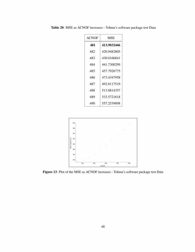
Table 20: MSE as ACNOF increases - Tohma’s software package test Data

ACNOF MSE

481 413.9032446

482 420.9482805

483 430.0166841

484 441.7300299

485 457.7926775

486 473.4347958

487 492.8117519

488 513.0814357

489 533.5721618

490 557.2539898

420

440

460

480

500

520

540

560

Mea

n S

quar

e E

rror

482 484 486 488 490

ACNOF

Figure 13: Plot of the MSE as ACNOF increases - Tohma’s software package test Data

48

Table 21: Summary of models estimations: Tohma’s software package test data

Models a or K MSE

Our model 481 413.9032446

HGDM (a) [17] 479 274.3

HGDM (b) [17] 497 242.4

HGDM (c) [17] 479 273.5

HGDM (d) [17] 497 242.5

HGDM (e) [17] 531 298.3

HGDM (f) [17] 476 566.3

HGDM (g) [17] 546 977.1

HGDM (h) [17] 497 364.3

HGDM (i) [17] 496 353.6

HGDM (j) [17] 498 371.8

HGDM (k) [17] 482 253.2

HGDM (l) [17] 486 328.7

S-Y Models 444.1965400 3843.008443

49

0

100

200

300

400

Num

ber

of F

aults

20 40 60 80 100 120

Debugging Day

Figure 14: Comparison of Tohma’s software package test Data set and our Predicted

50

2.5 Conclusions

In the present study we have introduced a logistic software reliability growth model for the purpose

of estimating the cumulative number of faults in a given software. The analytical form of this new

model is given by

L(t) =k

1 + me−bαt=

im


with

m = e−β0im

α = β1im


k = im and im the positive integer from N,N + 1, N + 2, ... at which MSEi is minimal.

This model not only gives very good predictions of the cumulative number of software faults, but it

is easy to apply and it is free of assumptions.

The new model was compared with the following commonly used models to in the subject area

i) Exponential Model

ii) G-O Model

iii) Delayed S-Shaped Model

iV) S-Y Models

V) C-Model

Vi) HGDM Hypergeometric Model

Vii) Huang, Kuo, Chen, and Lyu’s Models [5, 6, 7, 9]

We used seven different sets of actual data, namely,

i) the PL/I Database Application test data by Ohba,[10]

ii) Tohma’s software failure data, [11]

iii) the F 11-D program test data by Forman and Singpurwalla, [13]

iV) the pattern of discovery of errors STS2, STS3, STS4 by Misra [15]

V) the System T1 by Musa, [53]

51

Vi) the On-line data entry software test Data by Ohba,[10]

Vii) Tohma’s software package test Data, [11, 16, 18]

The mean square error criteria was used to compare the results of our proposed model with

other models stated above. The results presented in tables and graphical forms support the fact that

the new model is more effective in estimating the number of faults found during the testing and

debugging phase of a given software.

52

Chapter 3

Logistic Regression Approach to Software Reliability Assessment

3.1 Introduction

The increasing dependency on computers along with an increasing need for safety, efficiency and

cost reduction, causes not only for a higher demand for software and make software testing a crucial

phase of the development of any software to produce highly reliable packages. It is clear that an

air traffic control software will demand a very accurate failure behavior prediction, then a software

designed for a fun game. A crucial decision any software developer has to make, in software testing

and debugging phase, is the following: given all the restrictions, can we stop the testing and debug-

ging phase and release a software package for use, or should we continue testing?

Since the occurrence of software failures are random, if the testing and debugging team hits a long

random run where no software mistake is found; they are likely to stop testing and falsely conclude

that the software is error free. This leads to a premature end of the testing and debugging phase that

affect the reliability of the software to be released for marketing. Satoh and Yamada’s software reli-

ability growth models do not yield accurate reliability estimates in spite of a small amount of failure

data causing their procedure and justification do not lead to a good estimation at the early stage of

the testing and debugging phase. In this chapter, we propose a more realistic model that is more

effective and eliminates many of the difficulties that the S-Y models require. Our proposed software

reliability growth model is simple to implement and does not assume any prior distribution.

Relatively early in the testing and debugging phase, it provides accurate parameters estimation,

gives a very good failure behavior prediction and it is possible for software developers to predict

when to conclude testing, release the software and avoid over testing in order to cut the cost during

the development and the maintenance of the software.

The remaining of this Chapter is organized as follows: in Section 3.2 we summarize Satoh and

Yamada’s models, [1]. In Section 3.3, we present our proposed Logistic Early Estimation Model.

53

Comparison of the Logistic Early Estimation Model, LR-EE-Model, with several pre-existing mod-

els is made using real data from seven actual world problems in Section 3.4. Finally, our conclusions

and recommendations are given in Section 3.5.


• LR-EE-Model: our Logistic Regression Early Estimation Model

• S-Y Models: Satoh and Yamada’s Software reliability growth models

3.2 preliminaries

Here, we shall give a brief description of Satoh and Yamada statistical models.

3.2.1 Satoh and Yamada’s models and conclusions

Satoh and Yamada reported that, their two software reliability growth models yield accurate pa-

rameter estimates even with a small amount of data, [1]. Their proposed models give the same

parameters estimates. According to Satoh and Yamada, although the conventional model uses a dis-

crete equation as a regression model, the model itself is a continuous time model, thus, it includes

errors generated by discretization, however, their models do not have this problem because they are

themselves discrete models and that they can analyze the software reliability without a continuous

time model.

The Satoh and Yamada discrete models were reported to have three advantage over the conventional

model [1].

(1) The parameter estimation in the discrete logistic curve models reproduced the values of the

parameters very accurately, even with small data that do not include the inflection point. When

the exact solution is used as the input data, the conventional model provides inaccurate parameter

estimates with data that do not include the inflection point.

(2) The discrete models are independent of time scale. The same parameters estimates are ob-

tained no matter what value of the time scale they choose. When the conventional model is used we

have to choose the time scale carefully, because the time scale needs to be used in the regression

equation. As a result, the estimates depend on the choice of the time scale.

54

(3) The discrete logistic curve models enable them to accurately estimate the parameters in the

early testing phase with real data.

The parameter estimates of the conventional model vary with the number of data points. The dis-

crete models provide stable values of parameter estimates for various number of data points. This

characteristic is very important for software reliability growth models.

3.2.2 Remarks

we believe that Satoh and Yamada’s conclusion results from not simulating the data properly; they

use the exact solution is used as the input data not adding any noise. As a result, the problem is

purely deterministic. Since there are three parameters k, m, and α, to estimate in

L(t) = k1+m exp(−αt) , if no noise is added to an exact solution when preparing the data, as a Satu-

rated model one only needs as many data points as there are parameters to estimate the parameters.

While Satoh and Yamada’s approach perfectly reproduces the values of the parameters, when the

data set satisfy an exact solution with no noise, in early stage of the debugging and testing phase

(three data points), their parameter estimation with too small data points does not give accurate

parameter estimates on prepared data with noise and on actual data.

3.3 Development of The Proposed Model: Early Estimation

The crucial decision any software developer have to make, in software testing and debugging phase

is wether to stop, conclude the testing and the debugging phase of a software or continue testing

and debugging it. Having to take into consideration factors like reliability of the software being

developed and the cost of its development process, it is of gold for the software developers to have

a stopping rule, at the early stage of the testing and debugging phase, associated with a high confi-

dence level that testing and debugging phase must be concluded at some time t∗, to reduce cost of

over testing the software or that testing must proceed a bit longer to avoid a premature ending of the

debugging process to produce more reliable or highly reliable softwares.

The objective of this section is to develop a software reliability growth model that


(ii) is free of any major convergence assumptions

(iii) is simple

55

(iV) fits very well the cumulative number of software faults found and corrected

(V) provides accurate parameter estimates relatively early in the testing phase once the available

data points during testing and debugging phase include a bit more then the inflection point

(Vi) Our proposed model provides stable values of parameter estimates once the available data

includes a bit more then the inflection point; this characteristic is very important for software relia-

bility growth models.

(Vii) provides an additional decision-making rule to the software developers respective to when

to conclude the testing phase, manage their resources, and schedule the release time of the software

package to be marketed for use.

(Viii) not subject to errors generated by discretization.

(iX) our LR-EE-Model, by providing a stopping and release rule, saves time and cuts cost in

preventing over-testing the software to be marketed, and produces a more reliable software in pre-

venting an early release of the software to be market, specially when the testing and debugging team

hits a long run where not software fault is found.

3.3.1 Model Description

The description of our model is as proposed in Chapter 2, Section 2. The proposed model is

dependent on an accurate estimated number of software faults in the software k, before complete

modeling of the cumulative failure behavior is obtained. In this chapter, we propose a new way of

estimating the parameter k, as an increasing number of available failure data are recorded, while the

testing and debugging phase proceeds. Our new estimate of the parameter k is based on an accurate

method to locating the inflection point of a gradually increasing amount of actual failure data points.

Once the inflection point is located, a prediction of the total number of software faults k is obtained;

then estimation of the remaining parameters m and α is obtained, as proposed in

Chapter 2, by identification.

3.3.2 Parameters Estimation

Clearly, if k the initial number of software faults in the software prior the debugging phase or the

total number of software faults found and corrected in debugging phase during an infinitely long

exposure time interval, when a Cumulative logistic curve model is fitted, at the inflection point k2

56

software faults have been found and corrected. In this section, we propose a method for locating the

inflection point; then an estimate of k is found via estimating k2 .

Let T1 < T2 < T3 < ... < Tn be the first n successive random failure times, as software ages, with

their corresponding cumulative number of software faults found and corrected:

L(T1) = 1, L(T2) = 2, L(T3) = 3 , ..., L(Tn) = n.

We run sequential linear regression on two kind of successive overlapping chains of size N ordered

pairs (Ti, L(Ti) = i) that we will refer to as Chain 1 or Chain 2.

Description of overlapping chain I

Our chain I consists of overlapping chains of size N ≥ 2 constructed as follows:Our first run consist

of finding the equation of the regression on the first N ordered pairs (Ti , L(Ti) = i), i = 1, ..., N

and recording its slope; then for any other successive kth run k ≥ 2, we run a linear regression line

on (Ti , L(Ti) = i), where i = (k − 1)(N − 1), i + 2, i + 3, ..., i + N .

Description of overlapping chain II

Our chain II consists of overlapping chains of size N ≥ 4 and N is even, constructed as follows:

our kth run consists of finding the equation of successive regressions lines on the ordered pairs (Ti

, L(Ti) = i), where i = (k − 1)(N2 ) + 1, i + 1, i + 2, ..., i + (N − 1).

Locating the inflection point

For both successive overlapping chains of size N ordered pairs (Ti , L(Ti) = i), the slopes of the

successive regression lines are recorded and their patten is observed.

To locate the inflection point, we look for the chain on which the successive slope behavior is

maximal then consistently decreasing. Once the chain including the inflection point is identified,

averaging is used to estimate k.

(1) Select using the maximum slope criteria an ith chain

(2) In the selected ith chain, two times the actual cumulative faults is a candidate for k

(3) Test each candidate for k in the selected ith chain, using the minimum mean square error crite-

ria:

Let N , M , and three candidates from the selected ith chain such the N < M < L If MSEN >

57

MSEM , discard candidate N and proceed with comparing the mean square errors MSEMandMSEL

...

If MSEN < MSEN , select candidate N as the estimate of the parameter k.

After estimating k, we are ready to set up our Logistic Like Software Reliability Growth Model

proposed in Chapter 2.

Having an estimate of k, we name it k = iearly, we set up our best fit logistic like regression

model in the minimal mean square error sense.

proposing

P (t) =eβ0iearly

+β1iearlyt

1 + eβ0iearly

+β1iearlyt

to estimate the true cumulative percentage number of software failures found and corrected during

debugging and testing phase up to testing and debugging time t, we obtain estimates of m and α

needed in Equation 4. 9 as follows:

By identification method we obtain

11 + me−αt

≡ eβ0iearly

+β1iearlyt

1 + eβ0iearly

+β1iearlyt

=1

1 + 1

eβ0iearly e

β1iearlyt

=1

1 + e−β0iearly e

−β1iearlyt

(3. 1)

Now comparing the first and the last term of Equation 3. 1, we obtain the following estimates of

m and α:

m = e−β0iearly

α = β1iearly

where β0iearlyand β1iearly

are the Maximum Likelihood Estimators of the parameters β0 and β1,

using k = iearly and iearly the positive integer from N,M,L, ... at which slope is maximal and

mean square error is minimal .


P (t) =1

1 + me−bαt=

1

1 + e−β0iearly e

−β1iearlyt

58

Finally the cumulative failure behavior of the proposed model for a given software is given by

L(t) =k

1 + me−bαt=

iearly

1 + e−β0iearly e

−β1iearlyt

It will be shown that our proposed estimate of L(t) gives good results in comparison to the other

models that are commonly used.

3.4 Comparisons of Models: Numerical Application to Software Failure Data

In this section we shall illustrate our approach and compare the performance of our Early Estimation

Logistic Model, using overlapping chains, and using the mean square error, with several frequently

and pre-existing models on an actual software failure data already analyzed in

Chapter 2: the PL/I application program test data Table 1, on page 23 , reported and studied by

Ohba [10] in 1984.

It will be shown that our proposed model yields accurate parameters estimates early into the

testing and debugging phase, gives a very good modeling of the S-shaped cumulative number of

software faults found and corrected curves during testing and debugging phase giving the software

developers an early protocol as far as when to stop the testing and debugging phase and release the

software for use, cutting cost on maintenance, and due to over testing.

Our Early Estimation on the PL/I Software Failure Data

From Tables 22, Table 23, Table 24, and Table 25, respectively on pages 60, 61, 61, and 62, we

estimated a cumulative number of software fault of 350. Thus, our estimate K = 350.

Table 26, on page 63, provides a comparative summary of our estimate K along with several other

estimates from some pre-existing models and the mean square error for each model. Table 26 also

shows that by predicting 350 faults associated with an overall mean square error of 92.31760154 our

proposed model, LR-Model, without any major assumptions, fitting well trough the K-S goodness-

of-fit, demonstrates better performance than most of the pre-existing models when data points a bit

after the inflection points are available.

59

Creating Overlapping Chains: PL/I Database Application Software

Table 22: Overlapping Chain 1 of Size N = 2 -PL/I Database Application Software

RUNS [Ti, T(i+1)] [Ni, N(i+1)] slope of RL r

RUN 1 [1,3]; [15,66] 25.5 1

RUN 2 [2,4]; [44,103] 29.5 1

RUN 3 [3, 5]; [66,105] 19.5 1

RUN 4 [4, 6]; [103,110] 3.5 1

RUN 5 [5,7]; [105,146] 20.5 1

RUN 6 [6, 8]; [110, 175] 32.5 1

RUN 7 [7,9]; [146,179] 16.5 1

Note that only the data points up to the 9th week are use to predict the total number of faults in the

software.

60

Table 23: Overlapping Chain 1 of Size N = 2 -PL/I Database Application Software

N MSE Pair number

N= 88 6.61E-09 2

N=132 15.30759212 3

N=206 16.17930627 4

N=220 179.7683445 6

N=292 179.2839406 7

N = 350 165.1157652 8

N=351 165.259913

N=358 183.1532424 9

N=412 189.5550172 10

N=466 189.8825614 11

Table 24: Overlapping Chain 1 of Size N = 3-PL/I Database Application Software


RUN 1 [1,2,3]; [15,44,66] 25.5 r := .9968748929

RUN 2 [2,4 , 5]; [44,103,105] 21.64285714 r := .9539628928

RUN 3 [4, 6 ,7]; [103,110,146] 12.78571429 r := .8464894644

RUN 4 [6, 8,9 ]; [110,175,179] 24.35714286 r := .9605519477

RUN 5 [8,10,11]; [175,206,233] 18.78571429 r := .9887218045

Note that only the data points up to the 11th week are use to predict the total number of faults in

the software.

61

Table 25: Overlapping Chain 1 of Size N = 5-PL/I Database Application Software


RUN 1 [1,2,3,4,5] ; [15,44,66,103,105] 23.9 r := .9778998350

RUN 2 [4,6,7,8,9] ; [103,110,146,175,179] 17.33783784 r := .9416620919

RUN 3 [8,10,11,12,13]; [175,206,233,255,276] 20.60810811 r := .9952196625

Note that only the data points up to the 13th week are use to predict the total number of faults in

the software.

62

Table 26: Summary of models estimations: PL/I Database Application Software

Models a or K MSE AE

Our early estimation model 350 92.31760154 2.23

Our LR-Model 348 91.92380892 2.79

HLM Model Group A, with Logistic function 394.076 118.29 10.06

HLM Model Group A, with Weibull function 565.35 122.09 57.91

HLM Model Group A, with Rayleigh function 459.08 268.42 28.23

HLM Model Group A, with Exponential 828.252 140.66 131.35

HLM Model Group B, with Logistic function 337.41 163.095 5.75

HLM Model Group B, with Weibull function 345.686 91.0226 3.43

HLM Model Group B, with Rayleigh function 371.438 158.918 3.75

HLM Model Group B, with Exponential 352.521 83.998 1.53

HLM Model Group C, with Logistic function 430.662 103.03 20.11

HLM Model Group C, with Weibull function 385.39 87.5831 7.65

HLM Model Group C, with Rayleigh function 379.947 406.71 6.13

HLM Model Group C, with Exponential 385.179 83.3452 7.69

HLM Model Group D, with Logistic function 582.538 96.9321 62.72

HLM Model Group D, with Weibull function 958.718 124.399 167.79

HLM Model Group D, with Rayleigh function 702.693 247.84 96.09

HLM Model Group D, with Exponential 1225.66 169.72 242.36

G-O Model 562.8 157.75 56.98

Inflection S-Shaped Model 389.1 133.53 8.69

Delayed S-Shaped Model 374.05 168.67 4.48

Exponential Model 455.371 206.93 27.09

HGDM 387.71 138.12 8.3

Logarithmic Poisson Model NA 171.23

63

3.5 Conclusions

Modeling accurately the cumulative number of software faults k in a software package is crucial to

software developers. In the present study we have introduced a logistic software reliability growth

model for the purpose of early estimation of the cumulative number of faults in a given software.

The analytical form of this new model is given by

L(t) =k

1 + me−bαt=

iearly

1 + e−β0iearly e

−β1iearlyt

with

m = e−β0iearly

α = β1iearly

where β0iearlyand β1iearly

are the Maximum Likelihood Estimators of the parameters β0 and β1,

using k = iearly and iearly the positive integer candidate at which slope is maximum and at which

MSEi is minimal as the number of pairs increases.

This model not only gives very good predictions of the cumulative number of software faults, but it

is easy to apply and it is free of any major assumptions.


i) Exponential Model

ii) G-O Model

iii) Delayed S-Shaped Model

iV) S-Y Models

V) C-Model

Vi) Hypergeometric Model

Vii) Huang, Kuo, Chen, and Lyu’s Models [5, 6, 7, 9]

For a first application, we used one set of actual data, namely, the PL/I Database Application test

data by Ohba, [10]

Later we will apply our early estimation to the remaining sets analyzed in Chapter 2: i) the pattern

of discovery of errors test Data by Tohma, [11]

64

ii) the F 11-D program test data by Forman and Singpurwalla, [13]

iii) the pattern of discovery of errors STS2, STS3, STS4 by Misra [15]

iV) Musa’s System T1 V) the On-line data entry software package test Data by Ohba,[10]

Vi) A field report test Data by Tohma, [11, 16, 18]

The mean square error criteria was used to compare the results of our proposed model with other

models stated above. The results presented in tables form support the fact that the new model is

more effective in estimating the number of faults found during the testing and debugging phase of a

given software.

65

Chapter 4

Reliability Growth Model For Software Reliability

4.1 Introduction

There are usually four ways of characterizing failures that occurs when evaluating software pack-

ages, [52]:

1. time of failure

2. time interval between failures

3. cumulative failures experienced up to a given time

4. failures experienced in a time interval.

It is further understood that each of the above phenomena is being characterized by a random vari-

able.

In this Chapter we shall focus on predicting the time interval between failures for a given software

package. The Mean Time Between Failure (MTBF ) is the time difference between the expected

next failure time and current failure time. When working with softwares packages during their

development process, the mean time between failure (MTBF ) is a very important concept when

assessing the reliability of a given package after each modification. As a result, an accurate esti-

mation of the MTBF to predict the failure times of a given system is crucial when it comes to

planning corrective strategies.

As software faults are found and corrected during the testing and debugging phase, with the as-

sumptions discussed in Chapter 2, the reliability of the given software package increases meaning

that the time between failure of the software is expected to be relatively increasing in the long run.

Thus, the larger the time between failure (TBF ) the more reliable the software becomes. Most of

the existing models assume that the time between failures are exponentially distributed which make

them independent of time , [47]. When a dependency on time is exhibited, authors proposed the

66

nonhomogeneous Poisson process (NHPP ) to measure the reliability growth of the software and

make prediction about its failure behavior, [47]. Suresh and Rao developed a software reliability

growth model based on the NHPP with intensity function characterized by the inverse power law

process which uses an unbiased estimate of failure rate for prediction. The objective of this study is,

to develop a logistic model, to characterize the software reliability of a given package. A proposed

model to forecast the mean time between failures of a software package, after the last correction

has been implemented. Our proposed software reliability growth model offers the following advan-

tages:

(i) gives a very good mean time to next failure behavior prediction

(ii) provides accurate parameters estimation

(iii) it is simple to implement

(iV) the estimates are in closed form

(V) it is free of any major statistical assumptions

(Vi) tracks the failure rate with respect to increasing, decreasing or remaining constant.

In Section 4.2 we present an overview of a few models that are commonly used: Horigome-

Singpurwalla model, Mazucchi-Soyer model, Suresh-Rao model [47], and Quiao-Tsokos model,

[45]. In Section 4.3, we develop our logistic model to characterize behavior of the failures growth.

Comparison of our proposed model that we will refer to as LR-MTBF-Model with the commonly

used models is made using data from two real world problems in Section 4.4. Finally, our conclu-

sions and recommendations are given in Section 4.5.


• TBF: Time Between Failure

• Horigome-Singpurwalla model: H-M model

• Mazucchi-Soyer model: M-S model

• Suresh-Rao SRGM model: S-R SRGM model

• LR-MTBF-Model: our proposed model

•BEBE model: Mazzuchi and Soyer’s model

• SRGM: Software Reliability Growth Model

67

4.2 Preliminaries

Let Ti, i = 1, 2, 3, ..., n denote the age of the software as software faults are found and Yi,

i = 1, 2, 3, ..., n denote the life length of the software at the ith stage of testing following a modifi-

cation attempting to remove an error, [47]

Several models have been proposed for modeling the MTBF and estimating software failure times

when they can be characterized by the Power Law Process.

4.2.1 Bayes, Empirical-Bayes Model

Mazucchi and Soyer developed a Bayes Empirical-Bayes model using similar assumption as the

Littlewood-Verrall model, [38, 47].

Bayesian setting

Given Y1, Y2, Y3, Y4, ..., Yn.

1. The probability density function (pdf) of Yi is given by:

f(yi|λ) = λie−λiyi , yi > 0 (4. 1)

with failure rates depending on the stage of testing.

2. Given the failure rates at each stage of testing, the life-lengths of the software at each stage are

statistically independent.

3. The failure rates at each stage of testing are random variables. The pdf of λi is given by:

g(λi|α, β) =βα

Γ(α)λi

α−1e−βλi , λi > 0, α > 0, β > 0 (4. 2)

4. Given the parameters α and β, the failure rates at each stage of testing are statistically inde-

pendent.

5. Given the background information H , uncertainty of α and β is expressed via the prior

68

marginal pdf’s:

Π(α|H) =1u

0 < α < u (4. 3)

and

Π(β|H) =ba

Γ(a)βa−1e−bβ, β > 0 (4. 4)

where u > 0, a > 0, and b > 0 are known quantities.

6. Given background, the information H , α and β are statistically independent.

7. Given α, β, and (λ1, λ2, ..., λn), the Yi’s are statistically independent with each Yi statistically

independent of α, β, and all λ’s other than λi.

Computation of the posterior failures rates leads to integrals which cannot be expressed in closed

form, Lindley’s approximation, [47] is used to approximate the integrals. Mazucchi and Soyer’s

model was reported to be an improvement over the littlewood/Verrall model, after applying this

model to some actual software failure data first reported in [47].

4.2.2 Suresh-Rao SRGM

Suresh and Rao [47], extending the Nonhomogeneous Poisson Process to more appropriately de-

scribe the software failure process, developed a software reliability growth model with intensity

function characterized by the inverse power law (Weibull process). This intensity, characterized as

a function of the time , the number of errors found, and the time of occurrence of the last error, is re-

ported to allow them to consider increasing and decreasing software failure rate that tends to change

continually during test periods. Suresh and Rao’s model, was reported to give a significantly better

prediction of software reliability than Mazucchi and Soyer’s model and time series model ,[47].

Starting in the testing phase of the development of a software, the failure intensity is given by:

ν(t) = λδtδ−1, t > 0, λ > 0, δ > 0 (4. 5)

Letting Yi = Ti − Ti−1, i = 1, 2, ..., be the times between successive failures of the software. The

time to first failure is the Weibull distribution with failure rate as above [47]. Then for δ < 1, the

software is improving with time. The conditional distribution of Tk given Tk−1 , if ntk−1,tk is the

69

number of failure in the interval between tk−1 and tk, is given by:

Pr(Tk > tk|Tk−1 = tk−1) = Pr(ntk−1,tk) = exp(−∫ tk

tk−1

ν(t)dt) = exp(−λtδk+λtδk−1), tk ≥ tk−1

The joint density of T1, T2, ..., Tn is given by:

f(t1, t2, ..., tn) = (λδ)n exp[−λtnδ]

n∏

i=0

tδ−1i

Statistical inference procedures for the parameters λ and δ have been obtained by Crow, Flinkel-

stein, Lee and Lee, and by Engelhardt and Bain, [47]. From the likelihood function:

L(λ, δ; t1, t2, ..., tn) = (λδ)n exp[−λtδn]n∏

i=0

tδ−1i

The maximum Likelihood estimators of the parameters λ, and δ using T1, T2, ..., Tn are given by:

δ =n∑n

i=1 log(TnTi

)(4. 6)

λ =n

T δn

(4. 7)

The unbiased estimate of δ is derived to be:

δ = n−1n δ

Suresh obtained the unbiased estimate of νn:

νn =nδ

Tn

where δ is not defined for n = 0 and δ = 0 for n = 1.

reported the estimator of mean time to next failure at Tn to be:

1νn

.

70

4.2.3 Quiao-Tsokos Models

Quiao and Tsokos have formulated the basic structure of estimating the MTBF and the intensity

function for the Weibull process and derived bounds for estimating the expected time between the

nth and (n + 1)th failures given the time of the nth failure, [45].

Quiao and Tsokos developed a procedure for obtaining the best efficient estimate of a set of effi-

cient estimates for the Weibull Process. Then employed this statistical procedure to obtain the best

efficient estimate to the shape parameter of the Weibull process. Additionnally, the Linearly derived

best efficient estimates of the intensity function and its reciprocal when the Weibull process is being

used in reliability analysis. Quiao and Tsokos demonstrated the effectiveness of their statistical pro-

cedure analytically and numerically with several examples, using the concept of relative efficiency,

[45].

4.3 Development of The proposed Model

The objective of this section is to develop a software reliability growth model modeling the MTBF

to estimate software failure times, when the un-grouped cumulative number of software faults is

S-shaped, without deriving an intensity function required for the Power Law, that


(ii) gives a very good MTBF prediction in the MSE sense, providing better performance than

the pre-existing models

(iii) is simple and easy to implement

(iV) does not require any form of approximation

The very important of our proposed model allows software developers to connect time interval

between failures and cumulative failures experienced up to a given testing and debugging time,

giving them more details about the software failure data under study, to predict when a software is

ready to be released for use.

71

4.3.1 The Logistic Model

Let L(t) be the cumulative amount of software faults found and corrected in the debugging phase

during exposure time interval [0, t]. The parameter k (k > 0) represents the initial total number of

software faults in the software prior to the debugging phase as in Chapter 2 and in [1].

The logistic curve model is described by the differential equation

dL(t)dt

=α

kL(t)(k − L(t)), t ≥ 0 (4. 8)

where α (α > 0) and k (k > 0) are constant parameters to be estimated by regression analysis, [1].

Let

P (t) =L(t)k

Then, from Equation 4. 8, we have

dP (t)dt

= αP (t)(1− P (t)), t ≥ 0, P (0) =1

1 + m, m À k

where

P (t) =L(t)k

is the cumulative fraction number of software failures found and corrected in the debugging phase

during exposure time interval [0, t].

The solution of the above differential equation was noted to be

P (t) =1

1 + me−αt(4. 9)

where m is the constant of integration. Note that the graph of P (t) is S-shaped and 0 ≤ P (t) ≤ 1.

As developed in Chapter 2, we propose a Logistic Model to estimate the parameters k, m and α of

P (t).

72

4.3.2 Parameter Estimates

Following the proposed procedure in section 2.3 and plotting the estimated MSEi as i takes the

values i = N, N +1, N +2, ..., we propose on using an estimate of k, k where the minimum MSEi

occurs, that is, k = im, where im is one of the positive integers N,N +1, N +2, ... at which MSEi

is minimal.

Having the estimate of k, k = im, we propose

P (t) =eβ0im

+β1imt

1 + eβ0im+β1im

t

where β0im and β1im are the Maximum Likelihood Estimators of the parameters β0 and β1 as de-

scribe in chapter 2; P (t) given above estimates the true cumulative percentage number of software

failures found and corrected during debugging and testing phase up to testing and debugging time t.


P (t) =1

1 + me−bαt=

1


Finally the cumulative failure behavior of the proposed model for a given software was derive to be:

L(t) =k

1 + me−bαt=

im


4.3.3 Derivation of our proposed LR−MTBF Model

Starting with

L(t + h) ≈ L(t) + L′(t)h (4. 10)

and dividing both sides by k, we obtain the following approximation:

L(t + h)K

≈ L(t)k

+L′(t)

kh (4. 11)

which is equivalent to

P (t + h) ≈ P (t) + P ′(t)h (4. 12)

73

from which we obtain

P (t + h)− P (t) ≈ P ′(t)h (4. 13)

On the other hand, the probability that one software fault is found between t and t + h is given

by:

P (t + h)− P (t) =1k

(4. 14)

Combining the above equations gives

1k

= P (t + h)− P (t) ≈ P ′(t)h (4. 15)

from which we derive the following estimates:

1

k= P (t + h)− P (t) ≈ P ′(t)h (4. 16)

and obtain

h ≈ 1

kP ′(t)(4. 17)

Note that since

P (t) =eβ0im

+β1imt

1 + eβ0im+β1im

t

we differentiate P (t) to obtain

P (t)′=

β1imeβ0im+β1im

t

(1 + eβ0im

+β1imt)2

Finally, our proposed estimated (time between the nth and the n+1th failure) mean time to next

failure at time Tn is given by:

LR−MTBF (Tn) =1

kP ′(Tn)=

1

kP (Tn)′ =

(1 + eβ0im

+β1imTn

)2

imβ1imeβ0im+β1im

Tn(4. 18)

Note that our MTBT prediction depends on our estimate k of the total number of faults in

the Software. When at the end of a testing debugging phase we estimate that all the k faults in the

software were found and corrected, the MTBF get significantly large; in this case stop the MTBF

prediction at LR −MTBF (Tk−2). It will be shown that our proposed estimate of the mean times

between failure gives good results in comparison to the other models that are commonly used.

74

4.4 Comparisons of Models: Numerical Applications to Software Failure Data

After analyzing two actual failure data sets to compare their model with some pre-existing models in

terms of the mean square error, Suresh and Rao reported better performance of their model than the

Mazucchi-Soyer model (BEBE model), the Littlewood-Verral model, The Singpurwalla Horigome

model.

In this section we shall compare, using the mean square error, the Mazucchi-Soyer (BEBE), and

Suresh-Rao model to our proposed model on two sets of actual software failure data obtained from

actual projects. It will be shown to that our proposed model provides a very good modeling of

the mean time between failure, when un-grouped cumulative number of software faults found and

corrected during testing and debugging phase is S-shaped.

4.4.1 Apollo 8 software failure data: Comparison of the models


with the previous models, we analyze a data set, the Apollo 8 software test data given by Table 27,

on page 76 , that was first reported in Jelenski and Moranda in 1972, then studied by Verrall and Lit-

tlewood in 1973, by Mazuchi and Soyer in 1988 , by Suresh [47] in 1992, and re-visited by Roberts

in 2000, [26].

From Table 28, on page 77 ,after applying our model proposed in Chapter 2, we note that the mean

square error is minimal when the assumed cumulative number of failures is 28. Thus, our estimate

K = 28. Table 28 also shows that by predicting 28 faults associated with a mean square error of

0.269812501 along with the following estimates β0im = −3.1653and β1im = 0.0377

From the results summarized in Table 29, on page 79 , we note that with a MSE = 10.32 our pro-

posed model, LR-MTBF-Model, without any assumptions, demonstrates equal performance when

compared to the Suresh-Rao Model associated with a MSE = 10.34; and compared the the BEBE

Model with a MSE = 11.41 versus a MSE = 19.486 our proposed model demonstrates bet-

ter performance then the BEBE model. The advantage of our proposed model is that it not only

provides very good MTBF prediction when un-grouped cumulative failure behavior is S-shaped

Figure 16, on page 78, but it also give a very good cumulative software failure prediction Figure 15,

on page 78, and estimates the total number of fault in the software allowing the testing and debug-

ging team to decide when to release the software for use. Thus, our proposed model which is easier

75

to use and free of any major assumption gives very good if not better results then other models used

in industry.

Table 27: Apollo 8 Failure Data

Failure Number Actual TBF Actual Failure Time

1 9 9

2 12 21

3 11 32

4 4 36

5 7 43

6 2 45

7 5 50

8 8 58

9 5 63

10 7 70

11 1 71

12 6 77

13 1 78

14 9 87

15 4 91

16 1 92

17 3 95

18 3 98

19 6 104

20 1 105

21 11 116

22 7 123

23 2 125

24 1 126

76

Table 28: MSE as ACNOF increases - Apollo 8 data

ACNOF Mean Square Error

24 0.638528862

25 0.444854629

26 0.336156119

27 0.283498583

28 0.269812501

29 0.28087377

30 0.308914428

31 0.345979846

32 0.391210652

33 0.441151908

34 0.492927989

35 0.548889331

36 0.601757717

37 0.656688524

38 0.710669697

39 0.761844255

40 0.812992029

41 0.862548918

42 0.91197982

77

0.3

0.4

0.5

0.6

0.7

0.8

0.9

Mea

n S

quar

e E

rror

24 26 28 30 32 34 36 38 40 42

ACNOF

Figure 15: Plot of the MSE as ACNOF increases - Apollo 8 Failure data

5

10

15

20

25

Num

ber

of F

aults

0 50 100 150 200

Debugging Time

Figure 16: Comparison Of the Apollo 8 data set and our Predicted

78

Table 29: Actual and Predicted MTBF on the Apollo 8 data

Failure Number Actual TBF BEBE SRGM LRCRL

1 9 ..... ..... .....

2 12 10.53 ..... 17.94

3 11 11.84 8.89 12.15

4 4 11.79 9.01 8.75

5 7 9.64 6.12 7.83

6 2 9.15 5.92 6.53

7 5 7.85 4.47 6.23

8 8 7.44 4.3 5.57

9 5 7.55 4.81 4.77

10 7 7.27 4.64 4.41

11 1 7.27 4.87 4.06

12 6 6.66 4.13 4.02

13 1 6.62 4.26 3.85

14 9 6.16 3.72 3.84

15 4 6.39 4.24 3.8

16 1 6.23 4.11 3.86

17 3 5.89 3.7 3.88

18 3 5.71 3.55 3.96

19 6 5.56 3.43 4.06

20 1 5.59 3.58 4.36

21 11 5.35 3.3 4.42

22 7 6.84 3.85 5.35

23 2 9.73 4.04 6.24

24 1 9.39 3.84 6.55

Mean Square Error 19.486 11.41

Mean Square Error 20.27 10.33 10.32

79

Legend: Actual TBF-box BEBE model-circle S-R model-diamond Our model-cross

2

4

6

8

10

12

Fai

lure

Tim

e

5 10 15 20

Testing Stage

Figure 17: Comparison Of the Apollo 8 actual and Predicted MTBF

80

4.4.2 Musa’s Project 14C software failure Data: Comparison of models

Here, we shall compare our model effectiveness with the Suresh-Rao model that was reported to

perform better than the BEBE model that was an improvement over the Littlewood/Verall model.

We analyze a set of software reliability field data call project 14C test data given by Table 30,

on page 82, collected by John D. Musa of Bell Telephone Laboratories [52], to assist software

managers in monitoring test status and predicting schedules and to assist software researchers in

validating software reliability models. The project 14C, an application of Real time command and

control, is one of sixteen projects collected throughout the mid 1970s for which careful controls

were used during data collection to ensure that the data would be of high quality, [53]; Its size is

reported to be of hundreds of thousands delivered object code instructions. During the testing and

debugging phase 36 failures were found.

From Table 31, on page 83 , after applying our model proposed in Chapter 2, we note that the mean

square error is minimal when the assumed cumulative number of failures is 36. Thus, our estimate

K = 36 which agrees with the total the number of faults detected during actual debugging. Table 31

also shows that by predicting 36 faults associated with a mean square error of 3.094882808 along

with the following estimates β0im = −2.9125 and β1im = 4.829.10−7 .

From the results summarized in Table 32, on page 85, we note that with a MSE = 2.79596.1011

our proposed model, LR-MTBF-Model, without any assumptions, demonstrates better performance

when compared to the Suresh-Rao Model associated with a MSE = 6.68654.1011. Once again,

our proposed model not only provides very good MTBF prediction when un-grouped cumulative

failure behavior is S-shaped Figure 20, on page 86 , but it also give a very good cumulative software

failure prediction Figure 19, on page 84, and estimates the total number of fault in the software

allowing the testing and debugging team to decide when to release the software for use. Thus, our



81

Table 30: Musa’s Project 14C Data

F.N. F. I. L. Cum. F. T. F.N. F. I. L. Cum. F. T.

1 191520 191520 19 228315 5631060

2 2078820 2270340 20 51480 5682540

3 514560 2784900 21 44820 5727360

4 1140 2786040 22 850080 6577440

5 3120 2789160 23 361860 6939300

6 327480 3116640 24 39300 6978600

7 15420 3132060 25 545280 7523880

8 60000 3192060 26 256980 7780860

9 140160 3332220 27 396780 8177640

10 937620 4269840 28 91260 8268900

11 72240 4342080 29 1225620 9494520

12 737700 5079780 30 120 9494640

13 250680 5330460 31 1563300 11057940

14 2965 5333425 32 513000 11570940

15 196 5333621 33 177660 11748600

16 65173 5398794 34 2469000 14217600

17 2370 5401164 35 1678260 15895860

18 1581 5402745 36 170760 16066620

• F.N.: Failure Number

• F. I. L.: Failure Interval Lenght

• Cum. F. T.: Cumulative Failure Time

82

Table 31: MSE as ACNOF increases - Musa’s Project 14C Data

ACNOF Mean Square Error

36 3.094882808

37 3.959599606

38 4.928868157

39 5.931329159

40 6.942521785

41 7.92560927

42 8.878038857

43 9.791517534

44 10.66027927

45 11.47428189

46 12.25633147

83

4

6

8

10

12

Mea

n S

quar

e E

rror

36 38 40 42 44 46

ACNOF

Figure 18: Plot of the MSE as ACNOF increases - Musa’s Project 14C Data

5

10

15

20

25

30

35

Num

ber

of F

aults

0 2e+06 4e+06 6e+06 8e+06 1e+07 1.2e+07 1.4e+07 1.6e+07

Debugging Time

Figure 19: Comparison Of Musa’s Project 14C Data and our Predicted

84

Table 32: Actual and Predicted MTBF on Musa’s Project 14C Data

F. N. TBF S-R SRGM LR-MTBF F. N. TBF S-R SRGM LR-MTBF

1 191520 19 228315 237626.3298 235431.213

2 2078820 20 51480 233864.8431 232246.5118

3 514560 1332150014 478061.3697 21 44820 214988.3137 231726.4976

4 1140 1.61403E+11 402889.9732 22 850080 198190.1049 231332.4906

5 3120 1.597E+11 402744.7631 23 361860 248290.2288 234115.9895

6 327480 5605186548 402347.7938 24 39300 255329.8335 241329.7101

7 15420 1.21607E+11 364141.6983 25 545280 237020.0068 242340.8523

8 60000 91508318446 362503.4189 26 256980 257738.5758 261292.4014

9 140160 46698576008 356258.5331 27 396780 256089.2429 273653.5196

10 937620 3.54226E+11 342450.7742 28 91260 264275.4747 297622.1508

11 72240 40820287309 274280.3111 29 1225620 251414.6349 304049.2101

12 737700 2.18242E+11 270535.9194 30 120 314021.1506 432154.5279

13 250680 67724173.19 242450.5302 31 1563300 293094.1114 432171.6521

14 2965 54651909080 236742.4777 32 513000 373699.4164 771808.0491

15 196 55927419308 236685.7869 33 177660 382993.8163 953889.7591

16 65173 29415353580 236682.0481 34 2469000 370730.9139 1028352.278

17 2370 54349168455 235499.0811 35 1678260 502013.8426 3113131.758

18 1581 54698599781 235458.3178 36 170760 579874.5015 .....

S-R SRGM LR-LRT

MSE 6.68654E+11 2.79596E+11

• TBF: is the actual Time between Failure

• LR-MTBF: stands for our MTBF prediction

• S-R SRGM: stands for the Suresh-Rao MTBF prediction

• E + 11: 1011

85

Legend: Actual TBF-box S-R model-diamond Our model-cross

0

500000

1e+06

1.5e+06

2e+06

2.5e+06

3e+06

Fai

lure

Tim

e

5 10 15 20 25 30 35

Testing Stage

Figure 20: Comparison Of the Musa’s Project 14C actual and Predicted MTBF

86

4.5 Conclusion

In the present study we have introduced a logistic software reliability growth model for the purpose

of estimating the mean time between failure in a given software. The analytical form of this new

model is given by

MTBFL.R.S =1

kP ′(Tn)=

1

kP (Tn)′ =

(1 + eβ0im

+β1imTn

)2

imβ1imeβ0im+β1im

Tn(4. 19)


k = im and im the positive integer from N,N + 1, N + 2, ... at which MSEi is minimal, as pre-

sented in Chapter 2

This model not only gives very good predictions of the mean time to next failure, but it is easy to

apply and it is free of assumptions.


i) Mazzuchi and Soyer will be referred to as the Bayes Empirical-Bayes Exponential (BEBE) model.

ii) Suresh-Rao SRGM

We used two different sets of actual data, namely,

i) the Apollo 8 Software Failure Data

ii) Musa’s Project 14C software failure Data

The mean square error criteria was used to compare the results of our proposed model with other

models stated above. The results presented in tables and graphical forms support the fact that the

new model is more effective in estimating the mean time between failure during the testing and

debugging phase of a given software.

87

Chapter 5

Logistic Models using Bayesian procedures for Software Reliability

5.1 Introduction

Softwares a getting larger and larger thus becoming more and more complex. Although software

developers are not always able to test every software well enough to make them highly reliable,

highly reliable software are required to prevent catastrophes in several crucial areas like medical,

financial, defense, air traffic control, ...ect. Under the assumptions that once a software fault is found

it is corrected for good and that its correction does not introduce any new software faults. As a result,

we shall develop in this chapter two software reliability growth models, using Bayesian procedures.

The models are based on two difference equations proposed by Morishita and Hirota, each of which

is a discrete analog of the logistic curve model. As far as we can determine this is the first time

that these software reliability growth models Bayesian in nature are derived from two difference

equations discrete analogs of a logistic curve model proposed by Morishita and Hirota and used by

Satoh and Yamada, [1]. Section 5.2 provides the answer to the question: why do we go Bayesian?

and gives our underlying model.In Section 5.3, properties and advantages of the underlying model

are presented. In Section 5.4, we implement a Bayesian procedure and derive the Bayesian estimates

for the parameters of the underlying model. Application of the general Bayesian regression model is

applied to Morishita’s difference equation in Section 5.5. In Section 5.6, application of the general

Bayesian regression model is applied to Hirota’s difference equation. In section 5.7, we summarize

the quantities depending on the actual data that are involved in the Bayesian estimates for six of the

data sets previously studied in Chapter 2. Finally, our conclusions and recommendations are given

in Section 5.8.

88

5.2 Logistic Curve Model and Bayesian Regression Models

A logistic curve model is described as:

dL(t)dt

=α

kL(t)(k − L(t))

where L(t) is the cumulative number of software failures that occurred up to testing time t; α

(α > 0) and k, (k > 0) are constant parameters to be estimated by regression analysis. Recall

that the parameter k is the total number of software faults in the software before the testing and

debugging phase.

In this Chapter, we assume that parameter k is a constant and that parameter α behave like a random

variable with prior distribution π(α). α is directly proportional to the per capital growth rate at

which the software faults are found. The rate at which the mistakes are found depends on the

expertise of the tester, and the difficulty in modeling realistic testing processes (specially when

multiple testers are used) which introduce randomness enter the structure and cause the parameter

α to behave like a random variable.

Starting with Model I , as proposed by Satoh and Yamada,

yi = A + Bxi + εi i = (1, ..., n) (ModelI)

In order to generalize Model I to a Bayesian Regression Model, assume that parameters A and B

behave like random variables with joint prior distribution π(A, B) and that εi ∼ N(0, σ2).

Rewriting Model I , as follows, gives:

yi = (A + Bx) + B(xi − x) + εi (5. 1)

yi = β0 + β1zi + εi (ModelII) (5. 2)

with:

β0 = A + Bx

β1 = B

zi = xi − x

(5. 3)

89

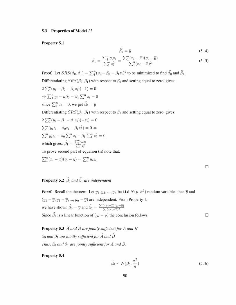
5.3 Properties of Model II

Property 5.1

β0 = y (5. 4)

β1 =∑n

1 yizi∑n1 z2

i

=∑n

1 (xi − x)(yi − y)∑n1 (xi − x)2

(5. 5)

Proof. Let SRS(β0, β1) =∑n

1 (yi − β0 − β1zi)2 to be minimized to find β0 and β1.

Differentiating SRS(β0, β1) with respect to β0 and setting equal to zero, gives:

2∑n

1 (yi − β0 − β1zi)(−1) = 0

⇔ ∑n1 yi − nβ0 − β1

∑n1 zi = 0

since∑n

1 zi = 0, we get β0 = y

Differentiating SRS(β0, β1) with respect to β1 and setting equal to zero, gives:

2∑n

1 (yi − β0 − β1zi)(−zi) = 0∑n

1 (yizi − β0zi − β1z2i ) = 0⇔

∑n1 yizi − β0

∑n1 zi − β1

∑n1 z2

i = 0

which gives: β1 =Pn

1 yiziPn1 z2

i

To prove second part of equation (ii) note that:∑n

1 (xi − x)(yi − y) =∑n

1 yizi

¤

Property 5.2 β0 and β1 are independent

Proof. Recall the theorem: Let y1, y2, ..., yn be i.i.d N(µ, σ2) random variables then y and

(y1 − y, y2 − y, ..., yn − y) are independent. From Property 1,

we have shown β0 = y and β1 =Pn

1 (xi−x)(yi−y)Pn1 (xi−x)2

Since β1 is a linear function of (yi − y) the conclusion follows. ¤

Property 5.3 A and B are jointly sufficient for A and B

β0 and β1 are jointly sufficient for A and B

Thus, β0 and β1 are jointly sufficient for A and B.

Property 5.4

β0 ∼ N(β0,σ2

n) (5. 6)

90

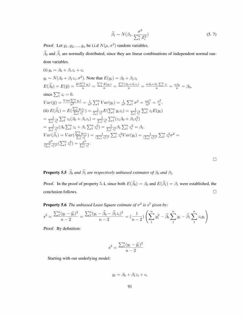
β1 ∼ N(β1,σ2

∑n1 Z2

i

) (5. 7)

Proof. Let y1, y2, ..., yn be i.i.d N(µ, σ2) random variables.

β0 and β1 are normally distributed, since they are linear combinations of independent normal ran-

dom variables.

(i) yi = β0 + β1zi + εi

yi ∼ N(β0 + β1zi, σ2). Note that E(yi) = β0 + β1zi

E(β0) = E(y) = E(Pn

1 yi)n =

Pn1 E(yi)

n =Pn

1 (β0+β1zi)n = nβ0+β1

Pn1 zi

n = nβ0

n = β0,

since∑n

1 zi = 0.

V ar(y) = V ar(Pn

1 yi)n2 = 1

n2

∑n1 V ar(yi) = 1

n2

∑n1 σ2 = nσ2

n2 = σ2

n .

(ii) E(β1) = E(Pn

1 yiziPn1 z2

i) = 1Pn

1 z2iE(

∑n1 yizi) = 1Pn

1 z2i

∑n1 ziE(yi)

= 1Pn1 z2

i

∑n1 zi(β0 + β1zi) = 1Pn

1 z2i

∑n1 (ziβ0 + β1z

2i )

= 1Pn1 z2

i(β0

∑n1 zi + β1

∑n1 z2

i ) = 1Pn1 z2

iβ1

∑n1 z2

i = β1.

V ar(β1) = V ar(Pn

1 yiziPn1 z2

i) = 1

(Pn

1 z2i )2

∑n1 z2

i V ar(yi) = 1(Pn

1 z2i )2

∑n1 z2

i σ2 =σ2

(Pn

1 z2i )2

(∑n

1 z2i ) = σ2Pn

1 z2i.

¤

Property 5.5 β0 and β1 are respectively unbiased estimator of β0 and β1.

Proof. In the proof of property 5.4, since both E(β0) = β0 and E(β1) = β1 were established, the

conclusion follows. ¤

Property 5.6 The unbiased Least Square estimate of σ2 is s2 given by:

s2 =∑n

1 (yi − yi)2

n− 2=

∑n1 (yi − β0 − β1zi)2

n− 2= (

1n− 2

)

(n∑

1

y2i − β0

n∑

1

yi − β1

n∑

1

ziyi

)

Proof. By definition:

s2 =∑n

1 (yi − yi)2

n− 2

Starting with our underlying model:

yi = β0 + β1zi + εi

91

since εi ∼ N(0, σ2) and E(yi) = β0 + β1zi we obtain:

yi = β0 + β1zi

andn∑

1

(yi − yi)2 =n∑

1

(yi − (β0 + β1zi))2 =n∑

1

(yi − β0 − β1zi))2

which gives:

n∑

1

(yi − yi)2 =n∑

1

y2i − β0

n∑

1

yi − β1

n∑

1

ziyi

Finally, we obtain:

s2 =

(∑n1 y2

i − β0∑n

1 yi − β1∑n

1 ziyi

)

n− 2

which complete the derivation.

¤

5.4 Implementing Bayesian procedures

5.4.1 Bayesian procedures on Model I

Using Model I , we have:

f(A, B|−→y ) = f(A, B|A, B)

f(A, B|A, B) = f(A, B|β0, β1) = f(β0, β1|A,B)π(A,B) = f(β0|A,B)f(β1|A,B)π(A,B)

where π(A,B) is the joint prior of parameters A and B that need not be independent which is a

disadvantage when using Model I . To avoid this problem, we propose working with Model II

5.4.2 Bayesian procedures on Model II

The posterior density is defined as:

f(β0, β1|−→y ) = f(β0, β1|β0, β1) =f(β0, β1|β0, β1).π(β0, β1)∫

f(β0, β1|β0, β1).π(β0, β1)dβ0dβ1

Now using Model II and its properties

starting with:

92

f(β0, β1|β0, β1)π(β0, β1)

Since β0 and β1 are independent it is reasonable to assume that β0 and β1 are independent and write:

f(β0, β1|β0, β1).π(β0, β1) = f(β0|β0, β1)f(β1|β0, β1).π(β0).π(β1)

Thus, the posterior density using Model II is:

f(β0, β1|−→y ) = f(β0, β1|β0, β1) =f(β0|β0, β1)f(β1|β0, β1).π(β0).π(β1)∫ ∫

f(β0|β0, β1)f(β1|β0, β1).π(β0).π(β1)dβ0dβ1

5.4.3 Derivation of the Bayesian estimates

With our underlying model

yi = β0 + β1zi + εi with εi ∼ N(0, σ2)

and using the Natural Conjugate prior approach, let’s assume that

π(β0) ∼ N(µ0, τ20 ) and π(β1) ∼ N(µ1, τ

21 )

where µ0, µ1, τ20 , and τ2

1 are provided by experts.

To obtain a close form for the Bayesian estimates, we work with the square error loss function.

Let’s denote the Bayesian estimates of β0 and β1 by β0B and β1B respectively, under the square

error loss function, we calculate the mean of the posterior density as follows:

β0B = E(β0|Data) = E(β0|β0, β1) =∫ ∫

β0f(β0|β0, β1)f(β1|β0, β1)π(β0)π(β1)dβ0dβ1∫ ∫f(β0|β0, β1)f(β1|β0, β1)π(β0)π(β1)dβ0dβ1

which is equivalent to:

β0B = E(β0|Data) ==∫

β0f(β0|β0, β1)π(β0)dβ0

∫f(β1|β0, β1)π(β1)dβ1∫

f(β0|β0, β1)π(β0)dβ0

∫f(β1|β0, β1)π(β1)dβ1

and similarly we obtain:

β1B = E(β1|Data) ==∫

β1f(β1|β0, β1)π(β1)dβ1

∫f(β0|β0, β1)π(β0)dβ0∫

f(β0|β0, β1)π(β0)dβ0

∫f(β1|β0, β1)π(β1)dβ1

with:

β0 ∼ N(β0,σ2

n)

93

β1 ∼ N(β1,σ2

∑n1 Z2

i

)

β0 ∼ N(µ0, τ0)

β1 ∼ N(µ1, τ1)

and our underlying model:

yi = β0 + β1zi + εi (5. 8)

is such that:

yi ∼ N(β0 + β1zi, σ2)

and

εi ∼ N(0, σ2)

We obtain:

β0B =

1(2π)4/2

1τ0τ1

σ√n

σ√Pi z2

i

∫∞−∞ β0e

− 12

(β0−β0)2

σ2n

+(β0−µ0)2

τ20

!

dβ0

∫∞−∞ e

− 12

0B@ (β1−β1)2

σ2Pi z2

i

+(β1−µ1)2

τ21

1CA

dβ1

1(2π)4/2

1τ0τ1

σ√n

σ√Pi z2

i

∫∞−∞ e

− 12

(β0−β0)2

σ2n

+(β0−µ0)2

τ20

!

dβ0

∫∞−∞ e

− 12

0B@ (β1−β1)2

σ2Pi z2

i

+(β1−µ1)2

τ21

1CA

dβ1

which simplify to:

β0B =

∫∞−∞ β0e

− 12

(β0−β0)2

σ2n

+(β0−µ0)2

τ20

!

dβ0

∫∞−∞ e

− 12

0B@ (β1−β1)2

σ2Pi z2

i

+(β1−µ1)2

τ21

1CA

dβ1

∫∞−∞ e

− 12

(β0−β0)2

σ2n

+(β0−µ0)2

τ20

!

dβ0

∫∞−∞ e

− 12

0B@ (β1−β1)2

σ2Pi z2

i

+(β1−µ1)2

τ21

1CA

dβ1

we note that

12

((β0 − β0)2

σ2

n

+(β0 − µ0)2

τ20

)=

12

((

1τ2

+1τ20

)β20 − 2(

β0

τ2+

µ0

τ20

)β0 + (β2

0

τ2+

µ20

τ20

)

)(5. 9)

Defining

ρ1 =1τ2

+1τ20

(5. 10)

94

and

τ2 =σ2

n(5. 11)

we obtain:12

[(β0 − β0)2

σ2

n

+(β0 − µ0)2

τ20

]

=12ρ1

[β2

0 −2ρ1

(β0

τ2+

µ0

τ20

)β0

]+

12(β2

0

τ2+

µ20

τ20

)

=12ρ1

[β0 − 1

ρ1(β0

τ2+

µ0

τ20

)

]2

− 12ρ1

(β0

τ2+

µ0

τ20

) +12(β2

0

τ2+

µ20

τ20

)

=12ρ1

[β0 − 1

ρ1(β0

τ2+

µ0

τ20

)

]2

+(β0 − µ0)2

2(τ20 + τ2)

Similarly, note that:

12

(β1 − β1)2

σ2Pi z2

i

+(β1 − µ1)2

τ21

=

12

((

1τ2

+1τ21

)β21 − 2(

β1

τ2+

µ1

τ21

)β1 + (β2

1

τ2+

µ21

τ21

)

)(5. 12)

Defining

ρ2 =1ν2

+1τ21

(5. 13)

and

ν2 =σ2

∑i z

2i

(5. 14)

we obtain:12

[(β1 − β1)2

σ2

n

+(β1 − µ1)2

τ21

]

=12ρ2

[β2

1 −2ρ2

(β1

ν2+

µ1

τ21

)β1

]+

12(β2

1

ν2+

µ21

τ21

)

=12ρ2

[β1 − 1

ρ2(β1

ν2+

µ1

τ21

)

]2

− 12ρ2

(β1

ν2+

µ1

τ21

) +12(β2

1

ν2+

µ21

τ21

)

=12ρ2

[β1 − 1

ρ2(β1

ν2+

µ1

τ21

)

]2

+(β1 − µ1)2

2(τ21 + ν2)

95

Thus,

β0B =

∫∞−∞ β0e

− 12ρ1

»β0− 1

ρ1(

β0τ2 +

µ0τ20

)

–2− (β0−µ0)2

2(τ20+τ2) dβ0

∫∞−∞ e

− 12ρ2

»β1− 1

ρ2(

β1ν2 +

µ1τ21

)

–2− (β1−µ1)2

2(τ21+ν2) dβ1

∫∞−∞ e

− 12ρ1

»β0− 1

ρ1(

β0τ2 +

µ0τ20

)

–2− (β0−µ0)2

2(τ20+τ2) dβ0

∫∞−∞ e

− 12ρ2

»β1− 1

ρ2(

β1ν2 +

µ1τ21

)

–2− (β1−µ1)2

2(τ21+ν2) dβ1

(5. 15)

Which simplify to:

β0B =

∫∞−∞ β0e

− 12ρ1

»β0− 1

ρ1(

β0τ2 +

µ0τ20

)

–2

dβ0

∫∞−∞ e

− 12ρ2

»β1− 1

ρ2(

β1ν2 +

µ1τ21

)

–2

dβ1

∫∞−∞ e

− 12ρ1

»β0− 1

ρ1(

β0ν2 +

µ0τ20

)

–2

dβ0

∫∞−∞ e

− 12ρ2

»β1− 1

ρ2(

β1ν2 +

µ1τ21

)

–2

dβ1

(5. 16)

equivalently, we obtain

β0B =

∫∞−∞ β0e

− 12ρ1

»β0− 1

ρ1(

β0τ2 +

µ0τ20

)

–2

dβ0

∫∞−∞ e

− 12ρ2

»β1− 1

ρ2(

β1ν2 +

µ1τ21

)

–2

dβ1

2π√ρ1ρ2

(5. 17)

then,

β0B =

√2π√

ρ−12√

2π√

ρ−12

∫∞−∞ β0e

− 12ρ1

»β0− 1

ρ1(

β0τ2 +

µ0τ20

)

–2

dβ0.√

2π√

ρ−11

2π√ρ1ρ2

(5. 18)

then,

β0B =

√2π

√ρ−12

[1ρ1

( β0

τ2 + µ0

τ20)].√

2π√

ρ−11

2π√ρ1ρ2

(5. 19)

which equate:

β0B of β0:

β0B =1ρ1

(β0

τ2+

µ0

τ20

)(5. 20)

Recalling that:

ρ1 =1τ2

+1τ20

=τ20 + τ2

τ20 τ2

(5. 21)

96

and

τ2 =σ2

n(5. 22)

Finally, after simplification, we obtain the following Bayesian estimate β0B of β0:

β0B =τ20

τ20 + σ2

n

β0 +σ2

n

τ20 + σ2

n

µ0

Now, similarly to the derivation of β0B , we derive β1B to be :

β1B =τ21

τ21 + σ2P

i z2i

β1 +σ2Pi z2

i

τ21 + σ2P

i z2i

µ1

Clearly, the Bayesian estimates of the parameters β0 and β1 are highly dependent on the choice

of the parameters of the prior distributions π(β0) and π(β1). To obtain suitable value for the param-

eters µ0, τ20 , µ1, and τ2

1 , we propose the following procedure:

5.5 Our Bayesian procedure on Morishita difference equation

Ln+1 − Ln =δα

kLn+1(k − Ln)

Rewriting as Model I:

Ln+1

Ln=

−δα

k(1− δα)Ln+1 +

11− δα

(5. 23)

(5. 24)

yn = BLn+1 + A (5. 25)

where:

yn = Ln+1

Ln

B = −δαk(1−δα)

A = 11−δα .

(5. 26)

97

Rewriting as Model II

Ln+1

Ln=

(1

1− δα− δα

k(1− δα)Ln+1

)− δα

k(1− δα)(Ln+1 − Ln+1

)+ εn (5. 27)

(5. 28)

yn = β0 + β1zn + εn (5. 29)

where:

β0 = 11−δα − δα

k(1−δα)Ln+1

β1 = − δαk(1−δα)

zn = Ln+1 − Ln+1

(5. 30)

Given the estimates of the regression coefficients, under our proposed Bayesian procedure, β0B and

β1B of the parameters β0 and β1 respectively,we can write:

β0B = 11−δα − δα

k(1−δα)Ln+1

β1B = − δαk(1−δα)

(5. 31)

where, α and k, respectively, our proposed estimates for the parameters α and k can be derive as

follows:

Starting with

β0B =1

1− δα+ β1BLn+1 (5. 32)

we derive our estimate α of the parameter α as follows:

11− δα

= β0B − β1BLn+1 (5. 33)

1

β0B − β1BLn+1

= 1− δα (5. 34)

δα = 1− 1

β0B − β1BLn+1

(5. 35)

α =1δ[1− 1

β0B − β1BLn+1

] (5. 36)

98

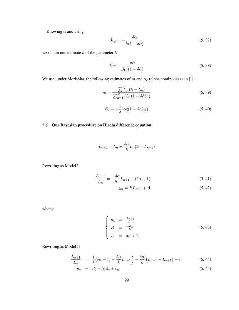
Knowing α and using

β1B = − δα

k(1− δα)(5. 37)

we obtain our estimate k of the parameter k

k = − δα

β1B (1− δα)(5. 38)

We use, under Morishita, the following estimates of m and αc (alpha continous) as in [1]:

m =∑N

n=1(k − Ln)∑Nn=1 (Ln(1− δα)n)

(5. 39)

αc = −1δ

log(1− δ ˆαdm) (5. 40)

5.6 Our Bayesian procedure on Hirota difference equation

Ln+1 − Ln =δα

kLn(k − Ln+1)

Rewriting as Model I:

Ln+1

Ln=−δα

kLn+1 + (δα + 1) (5. 41)

yn = BLn+1 + A (5. 42)

where:

yn = Ln+1

Ln

B = −δαk

A = δα + 1

(5. 43)

Rewriting as Model II

Ln+1

Ln=

((δα + 1)− δα

kLn+1

)− δα

k

(Ln+1 − Ln+1

)+ εn (5. 44)

yn = β0 + β1zn + εn (5. 45)

99

where:

β0 = δα + 1− δαk Ln+1

β1 = − δαk

zn = Ln+1 − Ln+1

(5. 46)

Given the estimates of the regression coefficients, under our proposed Bayesian procedure, β0B and

β1B of the parameters β0 and β1 respectively,we can write:

β0B = δα + 1− δαk

Ln+1

β1B = − δαk

(5. 47)

where, α and k, respectively, our proposed estimates for the parameters α and k can be derive as

follows:

Starting with

β0B = δα + 1 + β1BLn+1 (5. 48)

we derive our estimate α of the parameter α as follows:

δα = β0B − β1BLn+1 − 1 (5. 49)

α =1δ[β0B − β1BLn+1 − 1] (5. 50)

Knowing α and using

β1B = −δα

k(5. 51)

we obtain our estimate k of the parameter k

k = − δα

β1B

(5. 52)

We use, under Hirota, the following estimates of m and αc (alpha continous) as in [1]:

m =∑N

n=1(k − Ln)∑N

n=1

(Ln( 1

1+δα)n) (5. 53)

αc =1δ

log(1 + δαdh) (5. 54)

100

5.7 Numerical Application: Summary of the data dependent quantities

In this section we shall prepare six sets of actual software failure data obtained from actual projects,

already analyzed in Chapter 2, by evaluating all the actual data dependent quantities involved in the

proposed Bayesian estimates.

i) PL/I software Failure Data by Ohba,[10]

ii) Tohma’s Software Failure Data, [11]

iii) the F 11-D program test data by Forman and Singpurwalla, [13]

iV) Misra’s Space Shuttle Software Failure Data [15]

V) Musa’s System T1 software Failure Data

Vii) Tohma’s field report test Data [11, 16, 18]

we have listed the values needed for the calculation of our Bayesian estimates

values to be used in the Bayesian estimates for Data set 1

n = 18

∑

i

z2i = 161920.98

β0 = 1.235837821

β1 = −0.001422003

s2.... > σ2 = 0.199206243

Ln+1 = 199.9473684


n = 21

∑

i

z2i = 14335.3204

β0 = 1.397320307

101

β1 = −0.018307372

s2.... > σ2 = 1.006263898

Ln+1 = 53.81818182


n = 14

∑

i

z2i = 15210.9926

β0 = 1.229176596

β1 = −0.001399806

s2.... > σ2 = 0.082157217

Ln+1 = 66.46666667


n = 37

∑

i

z2i = 129179.97

β0 = 1.080216539

β1 = −0.000178343

s2.... > σ2 = 0.008896242

Ln+1 = 124.0789474

102


n = 18

∑

i

z2i = 38542.5842

β0 = 1.272513145

β1 = −0.001410044

s2.... > σ2 = 0.147405441

Ln+1 = 58.36842105


n = 110

∑

i

z2i = 2349985.9

β0 = 1.049033124

β1 = −0.000436099

s2.... > σ2 = 0.015019537

Ln+1 = 358.7387387

5.8 Conclusion

In the present study we have introduced two software reliability growth models that yield accurate

parameter estimates, using Bayesian procedures. The models are based on two difference equations

proposed by Morishita and Hirota, each of which is a discrete analog of the logistic curve model [1],

for the purpose of estimating the cumulative number of faults in a given software. The analytical

form of these two new models have been derived.

Working with the square error loss function, the Bayesian estimates derived are very sensitive to

the choice of the priors. As a result, after a careful investigation of the sensitivity of the obtained

103

Bayesian estimates with respect to the choice of the priors, we hope to be able to illustrate our ap-

proach and test its effectiveness.

104

Chapter 6

Future Work and Extensions

The present study enable us to identify several potential directions to extend and apply our results.

In this chapter, we shall briefly discuss some possible extensions for our research findings to more

realistic and useful analytical extensions.

In Chapter 2, we have developed of a simple, realistic, and easy to implement software reliability

growth model that provides a decision rule as of when to stop the testing and debugging phase and

release the software for use, for S-shaped cumulative software faults. We can use a Bayesian or

Quasi-Bayesian procedure in the present development of the proposed Model.

In Chapter 3, using the main feature of our proposed Model in Chapter 2- its inflection point, we

have proposed an effective method for estimating the number of faults in the software, at an early

stage of the testing and debugging phase. Our early estimation of the number of fault in the software

enable the software developers to plan the software development process, manage their resources

by avoiding cost due to over testing, make a software with higher reliability and decide when to

ship it for use. We need to develop a cost reduction analysis associated with our Early Estimation

proposed Model.

In Chapter 4, assuming a logistic model, we develop a procedure for predicting the mean time

between failure, after the last correction, of a software package creating a connection between pre-

dicting the MTBF and counting the cumulative failures experienced up to a given time. For the

prediction of the MTBF , one possible extension is to introduce a Bayesian or Quasi-Bayesian

procedure in the development of the proposed Model.

In Chapter 5, Using Bayesian procedures, we have developed two discrete software reliability

growth models based on two difference equations discrete analog of the logistic curve model re-

spectively proposed by Morishita and Hirota. we shall illustrated that the Bayesian Approach to

reliability is very useful modeling in understanding the final evaluation of a software package. One

of the key difficulties is to identifying and justifying the choice of the prior. Thus, we propose to

105

develop an Empirical Bayes approach to Software Reliability and thus bypassing having to assume

the choice of the prior. Furthermore, we extend to address the same problem from a nonparametric

point of view by utilizing Kernel Density estimation procedures to characterize the behavior of the

prior.

We also believe that formulating nonparametric Software Reliability models using the kernel den-

sity approach to characterize software failure would be of significant importance in cases where a

classical distribution cannot be identify to statistically fit the software failures.

106

References

[1] D. Satoh and S.Yamada, “Parameter Estimation of Discrete Logistic Curves Models for

Sofware Reliability Assessement,” Japan J. Indust. Appl. Math., 19(2002), 39− 53

[2] F. Morishita, “The fitting of the logistic equation to the rate of increase of population density,”

Res. Popul. Ecol. V II(1965), 52− 55

[3] “Computer science and statistics : proceedings of the Sixteenth Symposium on the Interface,”

Atlanta, 1984.

[4] D. W. Hosmer and S. Lemeshow, “Applied logistic regression,” John Wiley and Sons, NY,

1989.

[5] C. Y., J. H. Lo, and S.Y. Kuo, “Pragmatic study of Parametric Decomposition Models for Esti-

mating Software Reliability Growth,” Proc. 9th Int’l. Symp. Software Reliability Engineering

(ISSRE’98), 1998, pp. 111− 123.

[6] C. Y. Huang, S. Y. Kuo, and I. Y. Chen, “Analysis of a Software Reliability Growth Model with

Logistic Testing-Effort Function,” Proc. 8th Int’l. Symp. Software Reliability Engineering

(ISSRE’97), 1997, pp. 378− 388.

[7] C. Y. Huang, S. Y. Kuo, and M. R. Lyu, “Effort-Index-Based Software Reliability Growth

Models and Performance Assessment,” Proc. 24th Ann. Int’l. Computer Software and Appli-

cations Conf. (COMPSAC 2000), 2000.

[8] R. H. Hou, S. Y. Kuo, and Y. P. Chang, “Applying Various Learning Curves to Hyper-

Geometric Distribution Software Reliability Growth Model,” Proc. 5th Int’l. Symp. Software

Reliability Engineering, 1994, pp. 7− 16.

107

[9] S. Y. Kuo, C. Y. Huang, and M. R. Lyu, “Framework for Modeling Software Reliability, Using

Various Testing-Efforts and Fault-Detection Rates,” IEEE TRANSACTIONS ON RELIABIL-

ITY, VOL. 50, NO. 3, SPTEMBER 2001.

[10] M. Ohba, “Software reliability analysis models,” IBM J. Res. and Development, vol. 28, no.

4, pp. 428− 443, Jul. 1984.

[11] Y. Tohma , R. Jacoby, Y. Murata, and M. Yamamoto, “Hyper-Geometric Distribution Model

to Estimate the Number of Residual Software Faults,” Proc. COMPsac-89, Orlando, pp. 610−617, September 1989.

[12] Y. Tohma, H. Yamamoto and R. Jacoby, “Parameters Estimation of the Hyper-Geometric Dis-

tribution for Real/Test Data,” Proc. of the 18th International Symposium on Fault Tolerant

Computing, pp. 148− 153, 1988, Japan.

[13] E. H. Forman and N. D. Singpurwalla, “An Empirical Stopping Rule for Debugging and Test-

ing Computer Software,” J. American Statistical Association, Vol. 72, December 1977, pp.

750− 757.

[14] C. J. Dale and L. N. Harris: “Approach to Software Reliability Prediction,” Proc. Ann. Relia-

bility and Maintainability Symposium, pp. 167− 175, 1982.

[15] P. N. Misra: “Software reliability analysis,” IBM Systems Journal, Vol 22, NO 3, 1983.

[16] Y. Tohma, H. Yamano, M. Ohba, and R. Jacoby, “The Estimation of Parameters of the Hyper-

geometric Distribution and Its Application to the Software Reliability Growth Model,” IEEE,

1991.

[17] T. Doli, N. Wakana, S. Osaki, and K. S. Trivedi, “Analysis of Hypergeometric Distribution

Software Reliability Model,” IEEE, 2001.

[18] Y. Tohma, K. Tokunaga, S. Nagase, and Y. Murata, “Structural Approach to the Estimation of

the Number of Residual Software Faults Based on the Hyper-Geometric Distribution,” IEEE,

1989.

[19] M. A. Vouk: “Software Reliability Engineering,” 2000 Annual Reliability and Maintainability

Symposium.

108

[20] C. M. Bishop: “Bayesian Regression and Classification,” Advances in learning Theory: Meth-

ods, Models and Applications, J. A. K. Suykens et al. (Editors), IOS Press, NATO Science

Series III: Computer and Systems Sciences, volume ”190”.

[21] S. Yamada, J. Hishitani, and S. Osaki, “Software-Reliability Growth with a Weibull Test-

Effort: A Model and Application,” IEEE, 1993.

[22] El-Aroui: “A Bayes Nonparametric Framework for Software-reliability Analysis,” IEEE,

1996.

[23] Crow: “An Extended Reliability Growth Model For Managing And Assessing Corrective Ac-

tions,” IEEE, 2004.

[24] C. Y. Huang, C. T. Lin, S. Y. Kuo, M. R. Lyu, and C. C. Sue, “Software Reliability Growth

Models Incorporating Fault Dependency with Various Debugging Times Lags,” IEEE, 2004.

[25] “Computer science and statistics : proceedings of the Seventeenth Symposium on the Inter-

face,” Lexing, 1985.

[26] Roberts, H., “Predicting the Performance of Software Systems via the Power Law Process,”

Ph.D. Dissertation, University of South Florida, December 2000.

[27] Kjell A. Doksum, “Mathematical and statistical methods in reliability,” Bo H. Lindqvist, 2003.

[28] Isaac Elishakoff, “Safety factors and reliability : friends or foes?” Kluwer Academic Publish-

ers, Boston, 2004.

[29] J. D. Musa, “Software reliability data,” report and database available from: Data and Analysis

Center for Software; Rome Air Development Center (RADC), Rome, NY, USA.

[30] Bowyer, K.W., “Ethics and Computing: Living Responsibly in a Computrized World,” Los

Alamitos, CA: IEEE Computer Society Press, 1996.

[31] “proceedings annual Reliability and Maintainability Symposium,” Los Angeles, Ca., USA,

1982.

[32] Benington, H. D., “Production of Large Computer Programs”, in Proceedings, ONR Sympo-

sium on Advanced Programming Methods for Digital Computers, June 1956, pp. 15 − 27.

109

Reprinted in Proceedings, 9th International Conference on Software Engineering, Monterey,

CA, USA, March 30-April 2, 1987, pp. 299− 310.

[33] Scott H. Dick, “Computational intelligence in software quality assurance,” Ph.D. Dissertation,

University of South Florida, 2002.

[34] Bowyer, K. W., “Ethics and Computing: Living Responsability in a Computerized World”,

Los Alamitos, CA: IEEE Computer Society Press, 1996.

[35] Cai, K. Y., Wen, C.Y.; Zhang, M. L., “A critical review on software reliability modeling,”

Reliability Engineering and System Safety, vol. 32 no.3, 1991, pp. 357− 371.

[36] J. Higgins, C.P. Tsokos, “A quasi-bayes estimate of the failure intensity of a reliability growth

model,” IEEE Trans. Reliability, vol R-30, No.5, 1981, pp. 471− 475.

[37] M. Horigome, N.D. Singpurwalla, R. Soyer, “A Bayes Empirical Bayes Approach For ( Soft-

ware ) Reliability growth,” Computer Science and Statistics, The Interface, 1985, pp. 47− 55;

North Holland.

[38] B. Littlewood, J.L. Verrall, “A Bayesian reliability growth model for computer soft-

ware,”Applied Statistics vol 22, 1973, pp. 332− 346.

[39] G.J. Schick, R.W. Wolverton, “Assessment of software reliability,” Proceedings of Operations

Research, Physica- Verlag, Wurzburg-Wien, 1973, pp. 395− 422.

[40] Shimi, I. N. and Tsokos, C.P. (1977). “The Bayesian and nonparametric approach to reliability

studies: a survey of recent work”, in ” Proc. Of the Conf. On the Theory and Applications of

Relaibility With Emphasis on Bayesian and Nonparametric Methods,” vol.1, Acad. Press, New

York, pp. 5− 47.

[41] Tsokos, C., and Rao, A. (1994). “Estimation of Failure Intensity for the Weibull Process,”

Reliability Engineering and System Safety, 45 pp. 271− 275.

[42] Berger, J. (1985). “Statistical Decision Theory and Bayesian Analysis,” 2nd Edition, Springer-

Verlag, New York, Berlin, and Heidelberg.

110

[43] Canavos, G.C. (1972). “Bayesian approach to parameter and reliability estimation in the Pois-

son distribution,” IEEE Trans. Reliab.R-21, No. 1, 52-56.

[44] Ann Marie Neufelder, “Ensuring software reliability”, Marcel Dekker,Inc., NY, 1993.

[45] Qiao, H.; Tsokos, C.P., “Estimation of the three parameter Weibull probability distribution,”

Mathematics and Computers in Simulation, vol. 39, 1995, pp. 173− 185.

[46] Tsokos, C.P. et al. (1973). “Bayesian estimation of life parameters in the Weibull distribution,”

J. of Operations Research 21, No.3, pp. 755− 763.

[47] Nalina Suesh, “Modeling and analysis of software reliability”, Ph.D. Dissertation, University

of South Florida, 1992.

[48] F.W. Brefogle, “Statistical Methods for Testing, Development and Manufacturing,” John Wiley

and Sons, New York, NY (1991).

[49] H.F. Martz and R. A. Waller, “Bayesian Reliability Analysis,” John Wiley and Sons, New

York, NY (1982).

[50] V.K. Rohatgi, “An Introduction to Probability Theory and Mathematical Statistics,” Wiley

Eastern Limited (1990).

[51] Fellenburg, B. and Pilz, J. (1985). “On the choice of prior distribution for Bayesian reliability

analysis,”Freiberger Forsch D-170, 49− 68.

[52] John D. Musa, Anthony Iannino, Kazuh, “Software reliability : measurement, prediction,

application,” 1990.

[53] DACS, “DACS Software Reliability Dataset,”

http:// www.dacs.dtic.mil/datavases/sled/swel.shtml. Data and Analysis Center for Software .

[54] Everett, W.W.; Musa, J.D., “A software engineering practice,” IEEE Computer, vol. 26 no. 3

March 1993, pp. 77− 79.

[55] Farr, W., “Software Reliability Modeling Survey,” Handbook of Software Reliability Engi-

neering, New York: McGraw- Hill, 1996, pp. 71− 115.

111

[56] Friedman, M.A.; Voas, J. M., “Software Assessment: Reliability Safety, Testability,” New

York: John Wiley and Sons, Inc. 1995.

[57] Goel, A.L., “Software reliability models: assumptions, limitations, and applicability,” IEEE

Transactions on Software Engineering, vol. 11 no. 12, Dec. 1985, pp. 1411− 1423.

[58] Goel, A.L.; Okumoto, K., “Time -dependent error-detection rate model for software reliability

and other performance measures,” IEEE Transactions on Reliability, vol. 28 no. 3, August

1979, pp. 206− 211.

[59] Jelinski, Z.; Moranda, P.B., “Software reliability research,” in Proceedings, Statistical Com-

puter Performance Evaluation, November 22−23, 1971, Providence, RI, USA, pp. 465−484.

[60] Lewis, E.E., “Introduction to Reliability Engineering,” 2nd Ed., New York: John Wiley and

Sons , Inc., 1996.

[61] Lyu, M.R., Ed., “Handbook of Software Reliability Engineering,” New York: McGraw-Hill,

1996.

[62] Mazzuchi,T.A.; Soyer, R., “A Bayes-empirical Bayes model for software reliability,” IEEE

Transactions on Reliability, vol. 37 no.2, June 1988, pp. 248− 254.

[63] Wallace R. Blischke, D.N. Prabhakar Murthy, “Reliability : modeling, prediction, and opti-

mization,” 2000.

[64] Ross, S.M., “Software reliability: the stopping rule problem,” IEEE Transactions on Software

Engineering, vol. 11 no. 12, Dec. 1985, pp. 1472− 1476.

[65] Singpurwalla, N.D.; Soyer, R., “Assessing (software) reliability growth using a random coeffi-

cient autoregressive process and its ramifications,” IEEE Transactions on Software Engineer-

ing, vol. 11 no. 12, Dec. 1985, pp. 1456− 1464.

[66] Yamada, S.; Ohba, M.; Osaki, S., “S-shaped reliability growth modeling for software error

detection,” IEEE Transactions on Reliability, vol. 32 no. 5, Dec. 1983, pp. 475− 478.

[67] Yamada, S.; Osaki, S., “Software reliability growth modeling: models and assumptions,” IEEE

Transactions on Software Engineering, vol. 11 no. 12, Dec. 1985, pp. 1431− 1437.

112

About the Author

Louis Richard Camara was born in Dakar, Senegal, a french speaking country on the West coast

of Africa, on February 23, 1967. He came to the United States of America in September 1996

to pursue Mathematics studies at the University of South Florida. Louis, after completion of

an Accelerated BA/MA Program, received both his Bachelor’s degree (Magna Cum laude) in

Mathematics and his Master’s degree in Mathematics from the University of South Florida in

August 2001. He has been a Ph.D student in the Department of Mathematics at the University of

South Florida since the Fall of 2001. Louis is a member of The Golden Key and Phi Kappa Phi

honor societies.

statistical modeling and assessment of software reliability

Documents