statistical monitoring of the hand, foot and mouth disease...
TRANSCRIPT
Statistical Monitoring of the Hand, Foot and Mouth Disease in China 1
Statistical Monitoring of the Hand, Foot and Mouth Disease in China
Jingnan Zhang
Department of Biostatistics, University of Florida, Gainesville, 32611, USA
*email: [email protected]
and
Yicheng Kang
Department of Biostatistics, University of Florida, Gainesville, 32611, USA
*email: [email protected]
and
Yang Yang
Department of Biostatistics, University of Florida, Gainesville, 32611, USA
*email: [email protected]
and
Peihua Qiu
Department of Biostatistics, University of Florida, Gainesville, 32611, USA
*email: [email protected]
Summary: In a period starting around 2007, the Hand, Foot and Mouth Disease (HFMD) became wide-spreading
in China, and the Chinese public health was seriously threatened. To prevent the outbreak of infectious diseases like
HFMD, effective disease surveillance systems would be especially helpful to give signals of disease outbreaks as early
as possible. Statistical process control (SPC) charts provide a major statistical tool in industrial quality control for
detecting product defectives in a timely manner. In recent years, SPC charts have been used for disease surveillance.
However, disease surveillance data often have much more complicated structures, compared to the data collected
from industrial production lines. Major challenges, including lack of in-control data, complex seasonal effects, and
spatio-temporal correlations, make the surveillance data difficult to handle. In this paper, we propose a three-step
Biometrics 000, 000–000 DOI: 000
000 0000
procedure for analyzing disease surveillance data, and our procedure is demonstrated using the HFMD data collected
during 2008-2009 in China. Our method uses nonparametric longitudinal data and time series analysis methods to
eliminate the possible impact of seasonality and temporal correlation before the disease incidence data are sequentially
monitored by a SPC chart. At both national and provincial levels, our proposed method can effectively detect the
increasing trend of disease incidence rate before the disease becomes wide-spreading.
Key words: ARIMA model; Bootstrap; Disease surveillance and prevention; Early detection; Nonparametric
longitudinal data analysis; Statistical process control; Time series.
Statistical Monitoring of the Hand, Foot and Mouth Disease in China 1
1. Introduction
The Hand, Foot and Mouth Disease (HFMD) is a common infectious disease caused by a
group of non-polio enteroviruses that belongs to the Human Enterovirus species A (HEV-
A). Its main clinical symptoms include a brief prodromal fever followed by pharyngitis,
mouth ulcers and rash on the hands and feet. In most cases, the disease is mild and
self-limiting. However, severe clinical complications with neurological symptoms, such as
meningitis, encephalitis and polio-like paralysis, may occur (cf., Wang et al., 2011). In
2009, the number of HFMD cases reported in mainland China amounted to 1,155,525,
including 13,810 (or 1.2%) severe cases and 353 (or 0.03%) deaths. The high case-fatality
rate was attributed to reasons such as the rapid disease progression, late clinical treatment,
and limited local medical capacity. It was also found that the case-fatality rate decreased
considerably once the early clinical treatment was provided to patients with severe symptoms.
Therefore, effective disease surveillance and timely implementation of disease prevention and
control measures are critically important for minimizing the damage of HFMD (cf., World
Health Organization, 2011). This paper presents a case study of the HFMD data collected
in China during 2008-2009. It will show that certain statistical methods are helpful in early
detection of the HFMD outbreaks.
In the statistical literature, statistical process control (SPC) charts provide a major sta-
tistical tool for monitoring industrial production lines and for controlling product quality
(cf., Qiu, 2014). In recent several years, SPC charts have been frequently used for disease
surveillance and prevention (cf., Woodall, 2006). In this regard, some authors model the
number of disease incidents by a Poisson distribution and construct likelihood-ratio-based
control charts for disease monitoring (Zhou and Lawson, 2008). Some people develop control
charts based on parametric time series modeling of the possible temporal correlation in the
observed data (Watier, Richardson and Hubert, 1991). Some others propose multivariate
2 Biometrics, 000 0000
control charts to accommodate the spatial pattern exhibited by surveillance data (e.g., Jiang
et al., 2011, Rogerson and Yamada, 2004). However, disease surveillance data often have
much more complicated structures, compared to the data collected from industrial production
lines. Many issues about the observed disease incidence data need to be carefully addressed
before an SPC chart can be applied. For example, the Poisson distribution model and other
parametric distribution models are rarely valid in practice. The disease incidence often has
a complicated seasonal trend, and the conventional SPC chart cannot handle such a trend
properly. It is critically important to address all such issues properly in order to effectively
detect the HFMD outbreaks.
In this paper, we propose a three-step procedure for detecting HFMD outbreaks, and this
procedure is demonstrated using the HFMD data collected by the Chinese CDC during
2008–2009. Our proposed method consists of the following three steps:
(i) Detrend – Seasonality in the disease incidence data is first described by a nonparametric
longitudinal model, and is then eliminated from the observed data,
(ii) Decorrelation – Temporal autocorrelation in the detrended data is modeled by an ARIMA
model, and is then eliminated from the detrended data, and
(iii) Sequential Monitoring – The detrended and decorrelated data obtained in step (ii) are
then sequentially monitored by an SPC chart.
The remainder of this article is organized as follows. In Section 2, the HFMD data and the
proposed three-step procedure are described in more details, and the results of our analysis
of the HFMD data at the national level are also presented there. In Section 3, results of our
analysis for individual provinces are presented, and a data-driven procedure for searching for
the control limit of the SPC chart is discussed as well. Several remarks conclude the article
in Section 4.
Statistical Monitoring of the Hand, Foot and Mouth Disease in China 3
2. Nationwide Monitoring of HFMD
The data used in our analysis were collected by the HFMD reporting system in China from
December 2008 to November 2009. The system recorded the reporting times of diagnosed
HFMD cases and the locations of the reporting clinics nationwide in real time. Locations
of the reporting clinics were registered in the format of administrative code that consists
of 6 digits. Based on this code, we can identify administrative divisions of the country
at the village level and above. In this section, we combine the observed data of different
administrative divisions in the nation for monitoring HFMD at the national level. The
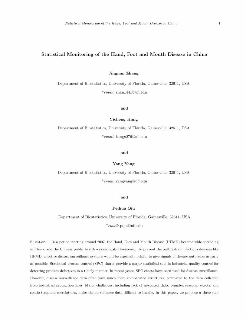
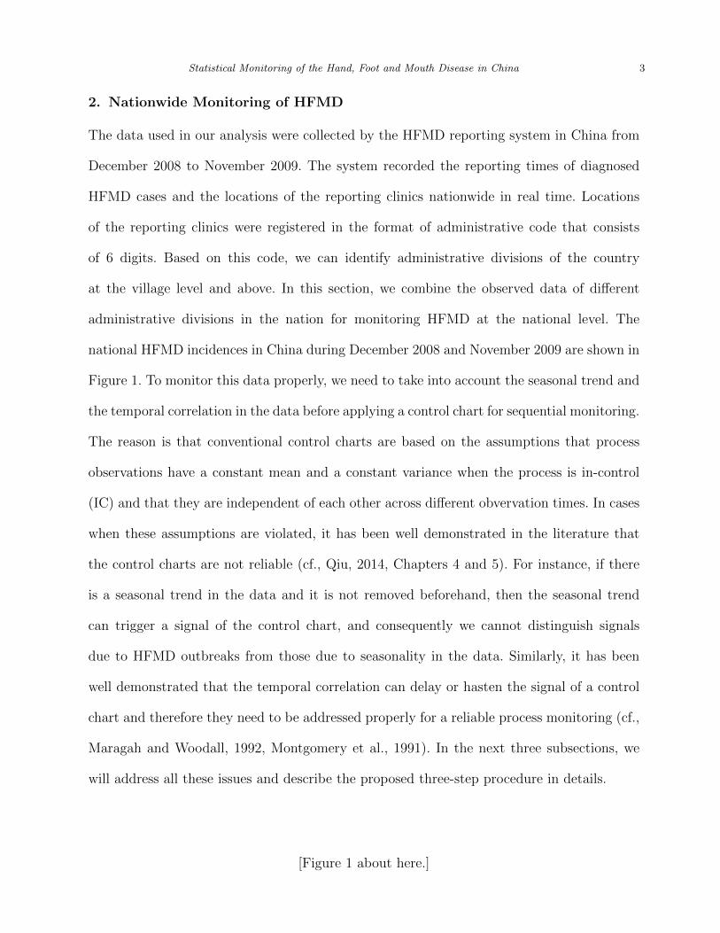
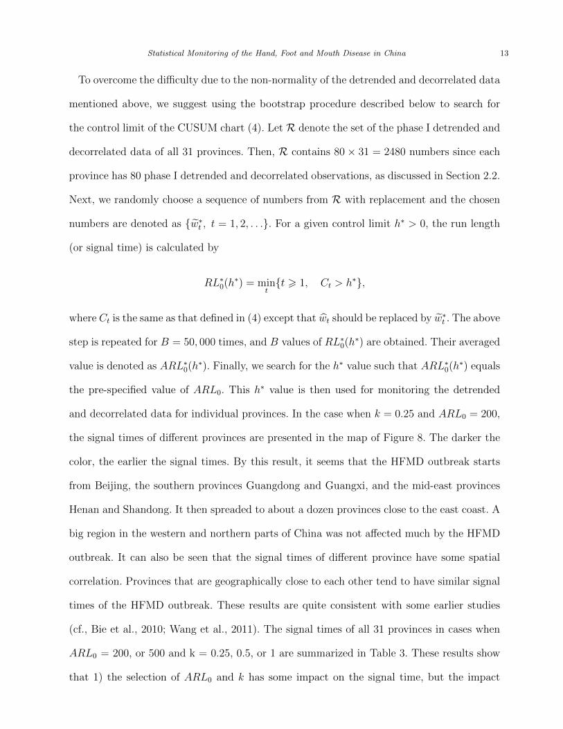
national HFMD incidences in China during December 2008 and November 2009 are shown in
Figure 1. To monitor this data properly, we need to take into account the seasonal trend and
the temporal correlation in the data before applying a control chart for sequential monitoring.
The reason is that conventional control charts are based on the assumptions that process
observations have a constant mean and a constant variance when the process is in-control
(IC) and that they are independent of each other across different obvervation times. In cases
when these assumptions are violated, it has been well demonstrated in the literature that
the control charts are not reliable (cf., Qiu, 2014, Chapters 4 and 5). For instance, if there
is a seasonal trend in the data and it is not removed beforehand, then the seasonal trend
can trigger a signal of the control chart, and consequently we cannot distinguish signals
due to HFMD outbreaks from those due to seasonality in the data. Similarly, it has been
well demonstrated that the temporal correlation can delay or hasten the signal of a control
chart and therefore they need to be addressed properly for a reliable process monitoring (cf.,
Maragah and Woodall, 1992, Montgomery et al., 1991). In the next three subsections, we
will address all these issues and describe the proposed three-step procedure in details.
[Figure 1 about here.]
4 Biometrics, 000 0000
2.1 Baseline Seasonal Trend
Like other infectious diseases, incidence of HFMD fluctuates over time and exhibits obvious
seasonal variation (Wang et al., 2011). Usually, such seasonal variation is not the main
interest of disease surveillance. In this subsection, we try to describe the seasonal variation
using a statistical model, and then remove it from the observed data for subsequent data
analysis. Ideally, the seasonal variation should be estimated from the observed data collected
in years when no disease outbreaks are present. Such data are called baseline data in
this paper. Unfortunately, Chinese government did not have a formal reporting system
for collecting HFMD incidence data before the outbreak took place in 2008. The lack of
such baseline data makes it challenging to accurately estimate the seasonal effect. However,
with the collected data at the provincial level, the following fact can be noticed. While
densely populated metropolitan areas (e.g., Beijing, Shanghai, etc.) were affected by HFMD
seriously during 2008-2009, the HFMD incident rates (defined to be the ratios of the numbers
of reported HFMD cases to the populations of the individual provinces) remain relatively
stable in some remote provinces. Thus, it is reasonable to use the data recorded in those
remote provinces to fit the baseline model. It should be pointed out that the incident rate
instead of the disease count is used here because different provinces have quite different
populations and the incident rate can adjust for the population properly.
To determine which province can be included in the baseline data, we use the following
criterion. For each province, its daily incident rates are calculated by dividing the daily
HFMD counts by its population. Then, the highest daily incident rate is obtained. If the
highest daily incident rate is below a threshold value, then that province is assumed to have
no HFMD outbreaks in the entire period of observation and that province can be included in
the baseline data. In this procedure, the population data of various provinces are obtained
from the official website of Chinese Census Bureau. Bie et al. (2010) estimated the average

Statistical Monitoring of the Hand, Foot and Mouth Disease in China 5
incidence rate of HFMD in China to be 0.0037 per 1,000 people in regular years when
no HFMD outbreaks exist. Therefore, we choose 0.0037 as the threshold value mentioned
above, based on which the following five provinces are included in the baseline data: Guizhou,
Xinjiang, Sichuan, Yunnan, and Tibet. Then, the average daily HFMD incidence rates of the
five provinces are computed and they are denoted as rt with t being the time. Assume that
rt follows the nonparametric regression model
rt = f(t) + εt, for t = 1, 2, . . . , n, (1)
where f(t) is a real-valued continuous function of t denoting the mean of rt, εt is the mean-0
error term, and n = 365 is the number of observations in the baseline data. Then, f(t) can
be used for describing the seasonal effect. The local quadratic kernel smoothing method (cf.,
Chapter 2, Qiu, 2005) is used for estimating f(t), in which the conventional Epanechnikov
kernel function is used and the bandwidth is chosen by the 10-fold cross-validation (CV)
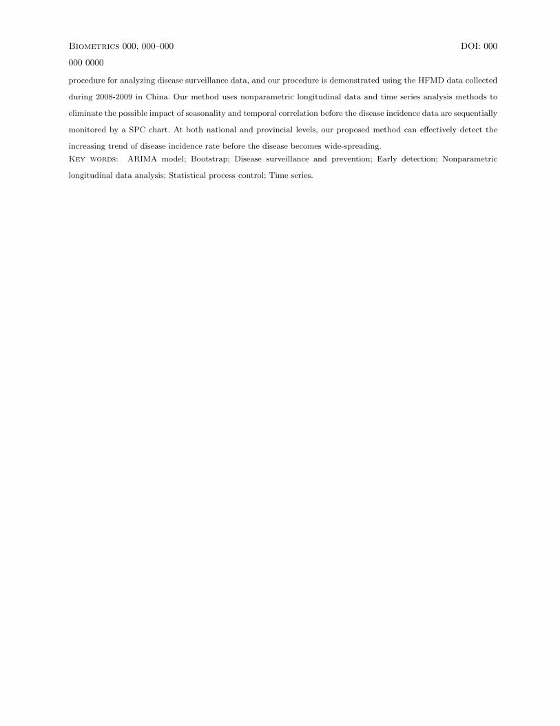
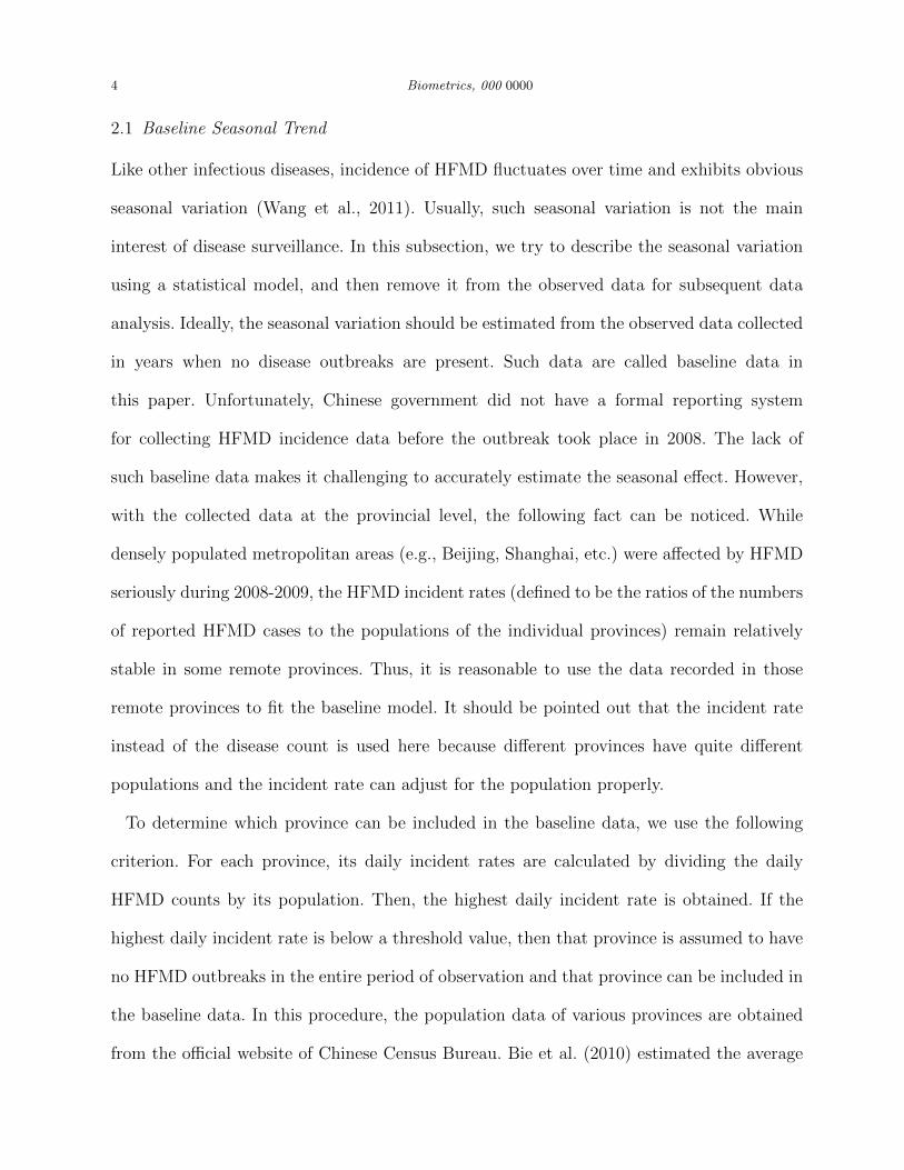
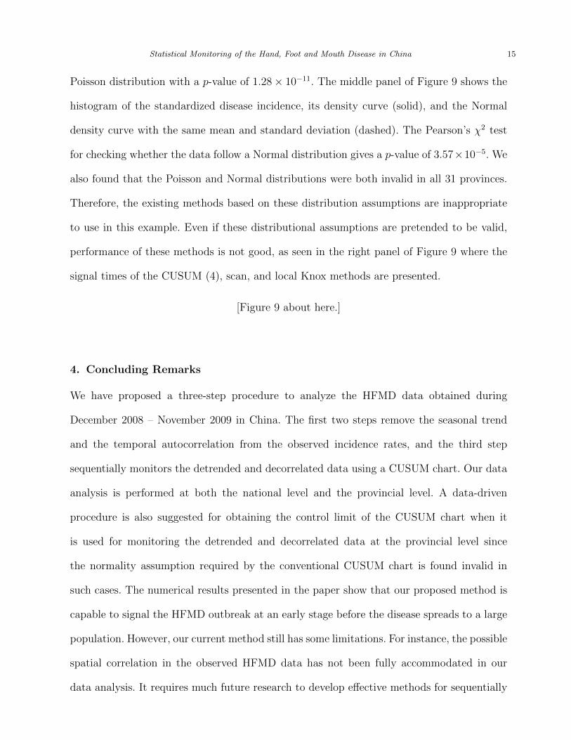
procedure. The estimated f(t), denoted as f(t), is shown in Figure 2 by the solid curve, with
the baseline data shown by the little circles. From the figure, we can see an obvious seasonal
pattern that the HFMD incidence is high in late spring and early summer, relatively low
in the autumn, and low in the winter. It should be pointed out that the autocorrelation is
not taken into account in this analysis for simplicity. The estimator f(t) can be regarded
as the local linear generalized estimating equations (GEE) estimator discussed in Lin and
Carroll (2000). The GEE estimator can accommodate autocorrelation without specifying
the autocorrelation structure by using the so-called independent working correlation matrix.
Under certain mild conditions, Lin and Carroll have shown that it is asymptotically the best
estimator. Therefore, f(t) should be an efficient estimator of f(t).
[Figure 2 about here.]
6 Biometrics, 000 0000
2.2 Temporal Correlation
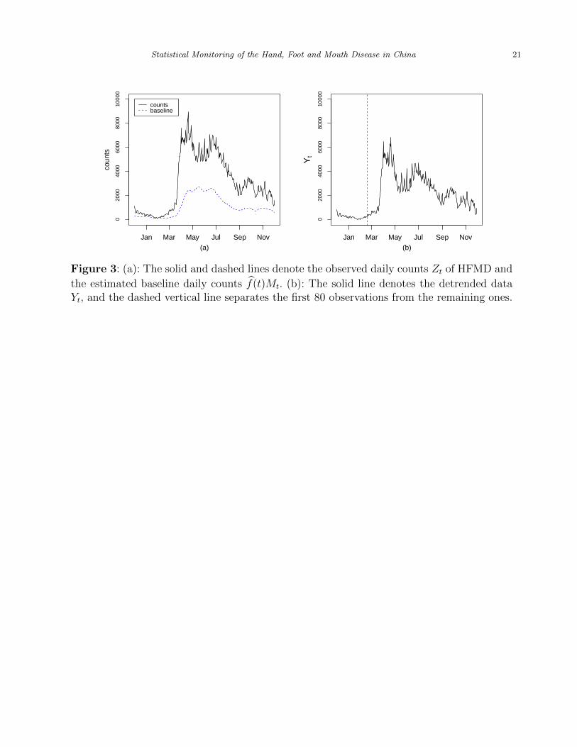
Let Zt be the national daily counts of HFMD. Define
Yt = Zt − f(t)Mt, for t = 1, 2, . . . , n, (2)
where f(t) is the estimated baseline incidence rate obtained from model (1), and Mt is the
national population at time t. Then, {Yt : t = 1, 2, . . . , n} can be interpreted as the daily
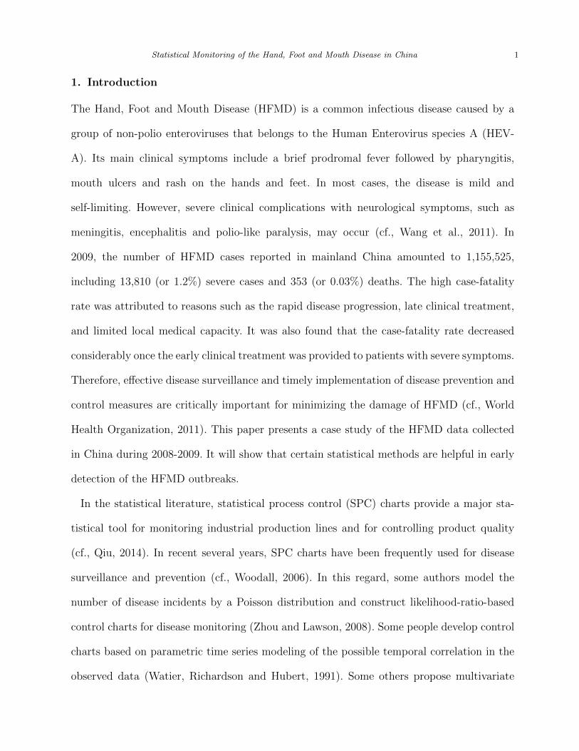
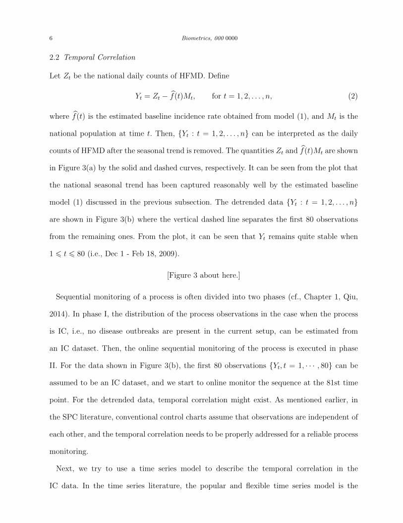
counts of HFMD after the seasonal trend is removed. The quantities Zt and f(t)Mt are shown
in Figure 3(a) by the solid and dashed curves, respectively. It can be seen from the plot that
the national seasonal trend has been captured reasonably well by the estimated baseline
model (1) discussed in the previous subsection. The detrended data {Yt : t = 1, 2, . . . , n}
are shown in Figure 3(b) where the vertical dashed line separates the first 80 observations
from the remaining ones. From the plot, it can be seen that Yt remains quite stable when
1 6 t 6 80 (i.e., Dec 1 - Feb 18, 2009).
[Figure 3 about here.]
Sequential monitoring of a process is often divided into two phases (cf., Chapter 1, Qiu,
2014). In phase I, the distribution of the process observations in the case when the process
is IC, i.e., no disease outbreaks are present in the current setup, can be estimated from
an IC dataset. Then, the online sequential monitoring of the process is executed in phase
II. For the data shown in Figure 3(b), the first 80 observations {Yt, t = 1, · · · , 80} can be
assumed to be an IC dataset, and we start to online monitor the sequence at the 81st time
point. For the detrended data, temporal correlation might exist. As mentioned earlier, in
the SPC literature, conventional control charts assume that observations are independent of
each other, and the temporal correlation needs to be properly addressed for a reliable process
monitoring.
Next, we try to use a time series model to describe the temporal correlation in the
IC data. In the time series literature, the popular and flexible time series model is the

Statistical Monitoring of the Hand, Foot and Mouth Disease in China 7
ARIMA (p,d,q) model (Box and Jenkins, 1976), where p, d, and q are three parameters, p
is the order of autoregression, q is the the order of moving average, and d is the order of
difference (see Shumway and Stoffer (2011) for their mathematical definitions). To estimate
the ARIMA model, we suggest selecting d using the successive KPSS unit-root test proposed
by Kwiatkowski et al. (1992) to determine the number of differences required for the time
series model to be stationary. The KPSS test is for testing the the null hypothesis that
the time series model is stationary. It proceeds as follows. First, a unit-root test (Dickey
and Fuller, 1979) is applied to {Yt : t = 1, 2, . . . , 80} to test whether the time series is
stationary using an autoregressive model. If the p-value of this test is smaller than a pre-
specified significance level α, then we proceed to run the unit-root test again on the first-order
differenced data {Yt+1−Yt, t = 1, 2, . . . , 80}. If the p-value is once again smaller than α, then
we continue to run the test on the second-order differenced data. This process continues
until obtaining the first insignificant p-value (i.e., p-value is bigger than or equal to α).
Throughout this paper, if no further specification, α is fixed at 0.05. Once d is determined,
p and q are chosen by minimizing some model selection criterion. Kwiatkowski et al. (1992)
suggested using the AICc criterion for selecting p and q, which is adopted in this paper.
After implementing the model estimation procedure described above, we choose the fol-
lowing ARIMA(1, 1, 0) model:
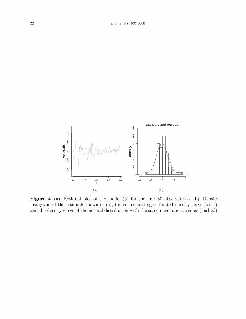
Yt+2 − Yt+1 = φ (Yt+1 − Yt) + wt, for t = 1, 2, . . . , 80, (3)
where wt’s are the i.i.d. random errors with mean 0 and unknown variance σ2w > 0. The
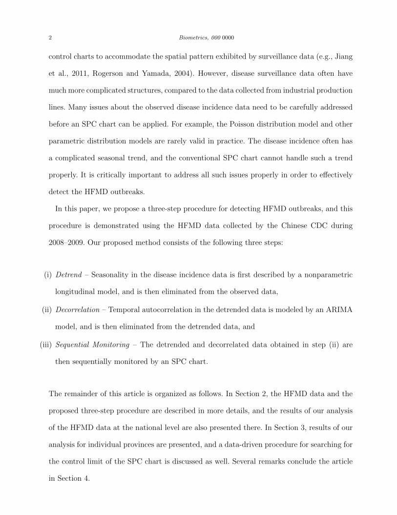
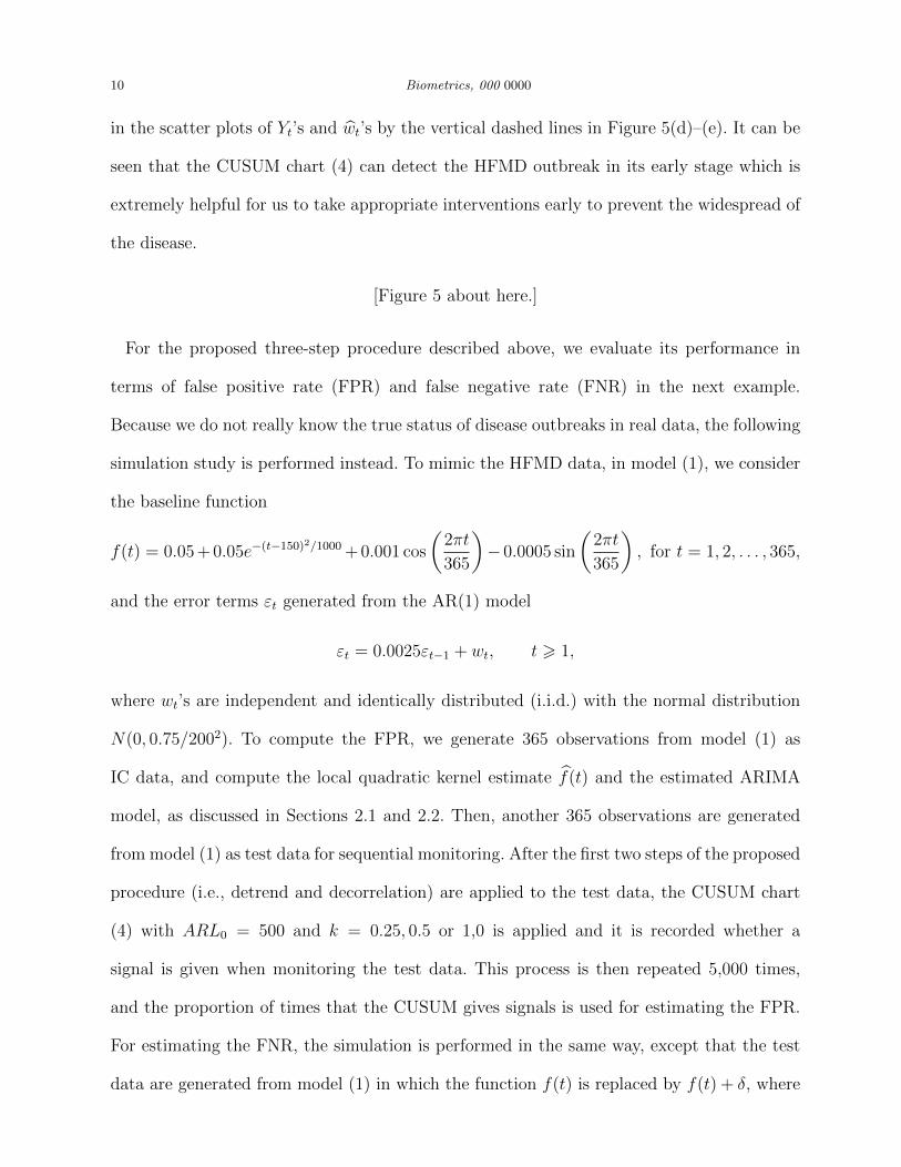
estimated value of φ is φ = 0.22. The standardized residuals of the fitted model (3) is shown
in Figure 4(a). If the model is appropriate, the residuals should look like the white noise
from a distribution with mean 0. One way to assess whether this is true is to perform the
Ljung-Box test (cf., Shumway and Stoffer, 2011). The p-value of the of Box-Ljung test in the
current case is 0.23, which indicates that the autocorrelation in {Yt : t = 1, 2, . . . , 80} has

8 Biometrics, 000 0000
been described well by (3) and there is no significant autocorrelation among the residuals
of the estimated model (3). The density histogram of the residuals shown in Figure 4(a),
the corresponding estimated density curve (solid line), and the density curve of the normal
distribution with the same mean and variance (dashed line) are shown in Figure 4(b). From
the plot, the distribution of the residuals is close to normal. As a matter of fact, the Shapiro-
Wilk normality test gives a p-value of 0.4413, which confirms that the distribution of the
residuals is not significantly different from normal.
[Figure 4 about here.]
2.3 Sequential Monitoring
After model (3) is estimated, the estimated model can be applied to the phase II detrended
data {Yt : t = 81, 82, . . . , n} to obtain the detrended and decorrelated phase II data {wt =
(Yt+2− Yt+1)− φ(Yt+1− Yt), t = 81, 82, . . . , n− 2}. If no HFMD outbreaks exist, then these
data should roughly follow a normal distribution with mean 0. Otherwise, the outbreaks will
be reflected in the mean shifts of {wt, t = 81, 82, . . . , n − 2}, as demonstrated by several
papers, including Jiang et al. (2000), Lu and Reynolds (2001), and Williamson and Hudson
(1999). Therefore, to detect the HFMD outbreaks, we can simply monitor the detrended and
decorrelated phase II data {wt, t = 81, 82, . . . , n− 2}. To this end, it has been well justified
that SPC charts (e.g., the Shewhart, CUSUM and EWMA charts) are effective tools (cf.,
Qiu, 2014). Because it has been justified that the IC distribution of {wt, t = 81, 82, . . . , n−2}
is close to a normal distribution and we are mainly concerned about upward shifts in the
HFMD incidence rates, we can consider using the classical CUSUM chart with the charting
statistic
Ct = max (0, Ct−1 + wt − k) , (4)

Statistical Monitoring of the Hand, Foot and Mouth Disease in China 9
where C0 = 0, and k > 0 is an allowance constant. The chart gives a signal of an upward
mean shift when
Ct > h,
where h > 0 is a control limit. In the SPC literature, k is usually chosen beforehand. It has
been well demonstrated that a larger k is good for detecting a larger shift, and a smaller k
is good for detecting a smaller shift. The chart (4) with a given k value, say k0, is optimal
for detecting the shift of size 2k0 in the sense that its out-of-control (OC) average run length
(ARL) is the shortest among all control charts with a given IC ARL value (Moustakides,
2004). Here, the IC ARL value is defined to be the average number of time points from the
beginning of process monitoring to the signal time when the process is IC, and the OC ARL
value is defined to be the average number of time points from the occurrence of a shift to
the signal time after the process becomes OC (cf., Section 4.2, Qiu, 2014). Therefore, the
concepts of the IC and OC ARL values are similar to the type-I error probability and power
in the hypothesis testing context. In practice, the IC ARL value is often specified beforehand,
and then a chart performs better if its OC ARL value is smaller when detecting a shift of a
given size. Commonly used IC ARL values include 100, 200, 370, 500, and 1000.
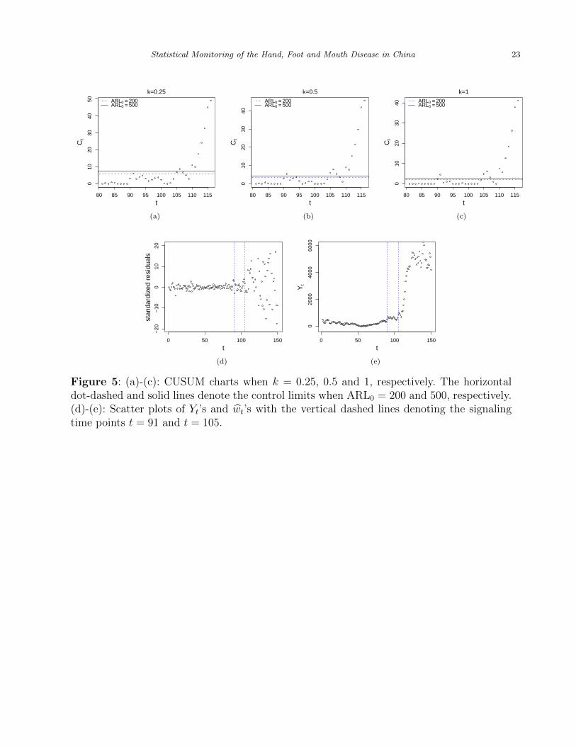
Next, we consider two commonly used IC ARL (denoted as ARL0) values 200 and 500, and
three k values 0.25, 0.5, and 1. For each combination of ARL0 and k, the corresponding value
of h can be computed numerically using either the existing R-packages, such as the package
spc, or a Monto Carlo simulation. The corresponding control charts are shown in Figure
5(a)–(c). From the plots, we can see that we have a convincing evidence of HFMD outbreaks
around the 105th time point (i.e., March 16 2009) for all values of ARL0 and k considered,
and the evidence of HFMD outbreaks around the 91st time point (i.e., March 1 2009) is only
marginally significant in cases when k = 0.5 and 1 and when k = 0.25 and ARL0 = 200. For
convenience of our perception, the two signaling time points t = 91 and t = 105 are plotted
10 Biometrics, 000 0000
in the scatter plots of Yt’s and wt’s by the vertical dashed lines in Figure 5(d)–(e). It can be
seen that the CUSUM chart (4) can detect the HFMD outbreak in its early stage which is
extremely helpful for us to take appropriate interventions early to prevent the widespread of
the disease.
[Figure 5 about here.]
For the proposed three-step procedure described above, we evaluate its performance in
terms of false positive rate (FPR) and false negative rate (FNR) in the next example.
Because we do not really know the true status of disease outbreaks in real data, the following
simulation study is performed instead. To mimic the HFMD data, in model (1), we consider
the baseline function
f(t) = 0.05 + 0.05e−(t−150)2/1000 + 0.001 cos
(2πt
365
)− 0.0005 sin
(2πt
365
), for t = 1, 2, . . . , 365,
and the error terms εt generated from the AR(1) model
εt = 0.0025εt−1 + wt, t > 1,
where wt’s are independent and identically distributed (i.i.d.) with the normal distribution
N(0, 0.75/2002). To compute the FPR, we generate 365 observations from model (1) as
IC data, and compute the local quadratic kernel estimate f(t) and the estimated ARIMA
model, as discussed in Sections 2.1 and 2.2. Then, another 365 observations are generated
from model (1) as test data for sequential monitoring. After the first two steps of the proposed
procedure (i.e., detrend and decorrelation) are applied to the test data, the CUSUM chart
(4) with ARL0 = 500 and k = 0.25, 0.5 or 1,0 is applied and it is recorded whether a
signal is given when monitoring the test data. This process is then repeated 5,000 times,
and the proportion of times that the CUSUM gives signals is used for estimating the FPR.
For estimating the FNR, the simulation is performed in the same way, except that the test
data are generated from model (1) in which the function f(t) is replaced by f(t) + δ, where

Statistical Monitoring of the Hand, Foot and Mouth Disease in China 11
δ denotes a constant shift. In this study, we consider δ = 0.005, 0.01, and 0.02. The results
are presented in Table 1.
[Table 1 about here.]
From Table 1, it can be seen that the FNR’s are quite small when δ = 0.01 and 0.02, and
they are relatively large when the shift is really small (i.e., δ = 0.005). Regarding the FPR’s,
they are between 17-34%. Besides the parameter k, we find that the bandwidth parameter
λ used in the local quadratic kernel estimation of f(t) also has an impact on the FNR and
FPR. To investigate this issue, besides the CV selection of λ, we also consider the cases when
λ = 0.1, 0.2, 0.3, and 0.4. The results are shown in Figure 6. From plot (a), it can be seen
that the FPR can be reduced a lot if we use a relatively large λ (e.g., λ = 0.3). In such cases,
the FNR would also be quite small if the true shift is small (e.g., δ = 0.02). So, in practice,
if we prefer a relatively small FPR, then λ should be chosen a little larger than the value
determined by the CV procedure.
[Figure 6 about here.]
3. Monitoring HFMD in Individual Provinces
In the previous section, we have demonstrated our proposed three-step procedure and used
it for monitoring the HFMD data at the national level. This preliminary analysis shows
that our method can detect the HFMD outbreak at an early stage. In practice, however, a
warning of the HFMD outbreak at the national level has a limited influence on the decisions
of local governments and local medical institutions regarding whether they should take
some preventive measures (e.g., quarantine infected patients or reduce public gatherings)
immediately after the national warning, since it is possible that only a few provinces are
in the danger of an HFMD outbreak in such cases. If the number of reported HFMD cases
remains relatively stable in a province, then such preventive measures would waste much

12 Biometrics, 000 0000
public resource. On the other hand, if a province is under imminent threat of an HFMD
outbreak, these preventive measures would be extremely important. Thus, it is necessary
to monitor HFMD outbreaks at a local level. In this section, we geographically divide the
HFMD data into thirty one groups, corresponding to the thirty one provinces in China,
and apply the proposed method at the provincial level. The method, however, can also be
used at a county or city level. The procedures for removing the seasonality and the temporal
autocorrelation remain the same as those described in Section 2, except that Mt in (2) should
be replaced by the population of each individual province. After using the ARIMA models
to decorrelate the detrended data at the provincial level, the estimated parameters of the
ARIMA models for individual provinces are listed Table 2. From the table, it can be seen that
there is some difference among different provinces in regard to the temporal autocorrelation
in the detrended data. But, the difference is quite small.
[Table 2 about here.]
However, our analysis shows that the distributions of the residuals of the fitted ARIMA
models (i.e., the detrended and decorrelated data) are significantly different from normal
distributions for most provinces. For instance, the histogram of the standardized residuals of
the estimated ARIMA(0,1,1) model for the Hebei province is shown in Figure 7, together with
the estimated density curve and the density curve of a standard normal distribution. From
the plot, it can be seen that the distribution of the residuals is skewed to the right, and the
Shapiro-Wilk normality test confirms that the distribution of the residuals is significantly
different from a normal distribution. In such cases, the control limits of the conventional
CUSUM chart (4) based on the normality assumption are invalid any more since the actual
IC ARL values of the chart would be quite different from the pre-specified nominal IC ARL
value in such cases (cf., Qiu and Hawkins, 2001; Qiu and Li 2011).
[Figure 7 about here.]
Statistical Monitoring of the Hand, Foot and Mouth Disease in China 13
To overcome the difficulty due to the non-normality of the detrended and decorrelated data
mentioned above, we suggest using the bootstrap procedure described below to search for
the control limit of the CUSUM chart (4). Let R denote the set of the phase I detrended and
decorrelated data of all 31 provinces. Then, R contains 80× 31 = 2480 numbers since each
province has 80 phase I detrended and decorrelated observations, as discussed in Section 2.2.
Next, we randomly choose a sequence of numbers from R with replacement and the chosen
numbers are denoted as {w∗t , t = 1, 2, . . .}. For a given control limit h∗ > 0, the run length
(or signal time) is calculated by
RL∗0(h
∗) = mint{t > 1, Ct > h∗},
where Ct is the same as that defined in (4) except that wt should be replaced by w∗t . The above
step is repeated for B = 50, 000 times, and B values of RL∗0(h
∗) are obtained. Their averaged
value is denoted as ARL∗0(h
∗). Finally, we search for the h∗ value such that ARL∗0(h
∗) equals
the pre-specified value of ARL0. This h∗ value is then used for monitoring the detrended
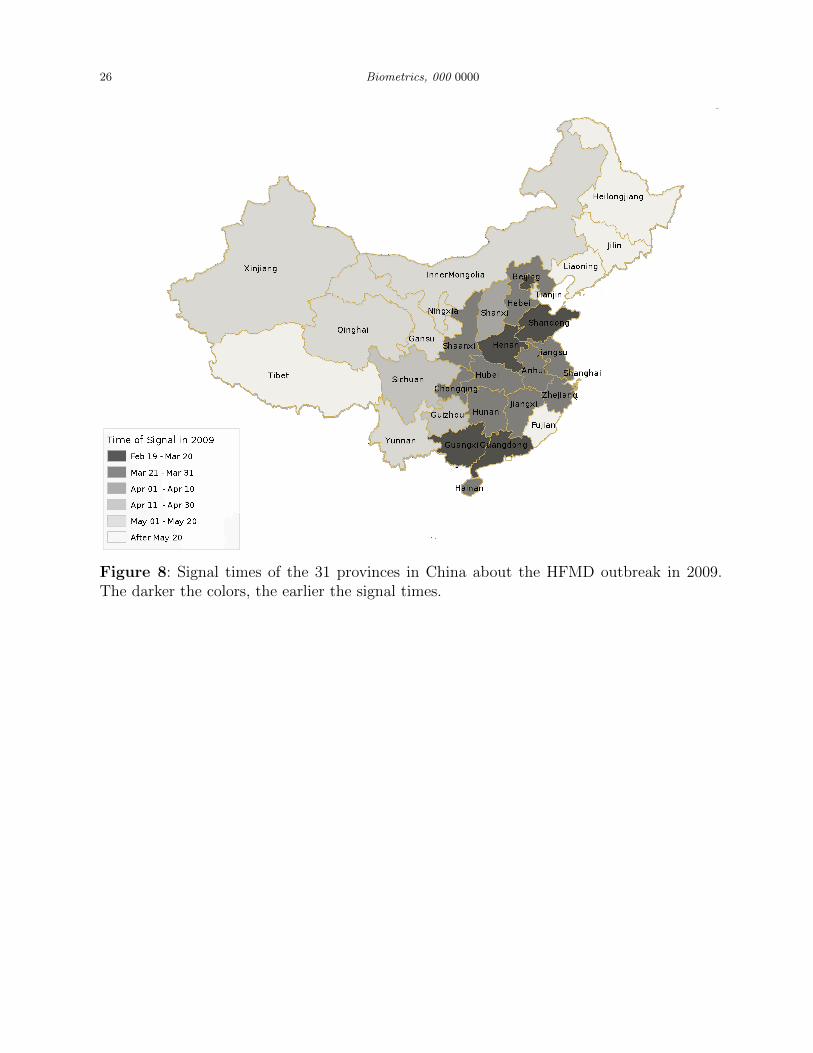
and decorrelated data for individual provinces. In the case when k = 0.25 and ARL0 = 200,
the signal times of different provinces are presented in the map of Figure 8. The darker the
color, the earlier the signal times. By this result, it seems that the HFMD outbreak starts
from Beijing, the southern provinces Guangdong and Guangxi, and the mid-east provinces
Henan and Shandong. It then spreaded to about a dozen provinces close to the east coast. A
big region in the western and northern parts of China was not affected much by the HFMD
outbreak. It can also be seen that the signal times of different province have some spatial
correlation. Provinces that are geographically close to each other tend to have similar signal
times of the HFMD outbreak. These results are quite consistent with some earlier studies
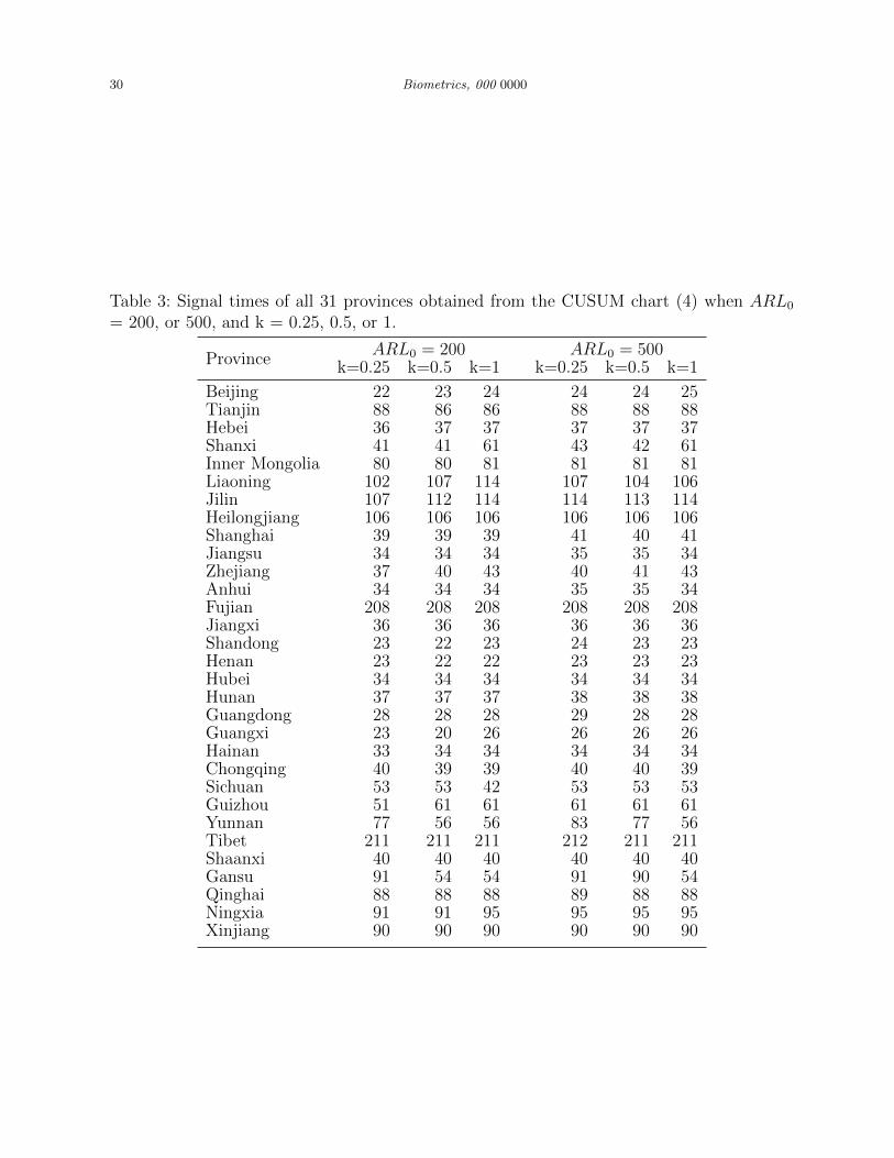
(cf., Bie et al., 2010; Wang et al., 2011). The signal times of all 31 provinces in cases when
ARL0 = 200, or 500 and k = 0.25, 0.5, or 1 are summarized in Table 3. These results show
that 1) the selection of ARL0 and k has some impact on the signal time, but the impact

14 Biometrics, 000 0000
is relatively small, and 2) the geographical pattern shown in the table matches with the
geographical pattern in Figure 8 well. The only provinces in which the signal times are quite
different when k changes are Yunnan and Gansu. After checking the data carefully, we found
that the number of HFMD cases had a single-day jump in Yunnan on April 15, 2009, and
it had a single-day jump in Gansu on April 13, 2009. In the literature, it has been well
desmonstrated that CUSUM charts with a larger k will be more effective to detect transient
shifts because the CUSUM charting statistic Ct defined in (4) uses less history data in such
cases (i.e., it is reset to be 0 more often in the “max” operation in (4)). See Section 4.2
in Qiu (2014) for a detailed discussion. Therefore, the chart (4) can react to the single-day
jump better when k is chosen larger. This explains why the signal times are shorter when k
is chosen larger for Yunnan and Gansu in Table 3.
[Figure 8 about here.]
[Table 3 about here.]
For the above HFMD data, we also tried the sequential monitoring scheme by Marshall
et al. (2007) that was based on the local Knox statistic proposed by Rogerson (2001), and
the space-time scan method by Kulldorff (2001). Marshall et al. (2007) argued that their
prospective monitoring scheme would be more effective than the original retrospective space-
time method using the local Knox statistic. Their method assumed that the standardized
disease incidence followed a normal distribution. The scan method, on the other hand,
assumed that the disease incidence in a local region and within a time interval followed a
Poisson distribution. In the HFMD example, the density histogram of the disease incidence
in the Jilin province is shown in the left panel of Figure 9, where the solid and dashed
curves denote the density curve of the data and the Poisson density with the same mean
and standard deviation. It can be seen that the two curves are quite different. The Pearson’s
χ2 test shows that the distribution of the disease incidence is significantly different from the
Statistical Monitoring of the Hand, Foot and Mouth Disease in China 15
Poisson distribution with a p-value of 1.28× 10⁻¹¹. The middle panel of Figure 9 shows the
histogram of the standardized disease incidence, its density curve (solid), and the Normal
density curve with the same mean and standard deviation (dashed). The Pearson’s χ2 test
for checking whether the data follow a Normal distribution gives a p-value of 3.57×10⁻⁵. We
also found that the Poisson and Normal distributions were both invalid in all 31 provinces.
Therefore, the existing methods based on these distribution assumptions are inappropriate
to use in this example. Even if these distributional assumptions are pretended to be valid,
performance of these methods is not good, as seen in the right panel of Figure 9 where the
signal times of the CUSUM (4), scan, and local Knox methods are presented.
[Figure 9 about here.]
4. Concluding Remarks
We have proposed a three-step procedure to analyze the HFMD data obtained during
December 2008 – November 2009 in China. The first two steps remove the seasonal trend
and the temporal autocorrelation from the observed incidence rates, and the third step
sequentially monitors the detrended and decorrelated data using a CUSUM chart. Our data
analysis is performed at both the national level and the provincial level. A data-driven
procedure is also suggested for obtaining the control limit of the CUSUM chart when it
is used for monitoring the detrended and decorrelated data at the provincial level since
the normality assumption required by the conventional CUSUM chart is found invalid in
such cases. The numerical results presented in the paper show that our proposed method is
capable to signal the HFMD outbreak at an early stage before the disease spreads to a large
population. However, our current method still has some limitations. For instance, the possible
spatial correlation in the observed HFMD data has not been fully accommodated in our
data analysis. It requires much future research to develop effective methods for sequentially

16 Biometrics, 000 0000
monitoring the spatio-temporal patterns of the disease incidence and for early detection and
prevention of the disease outbreak.
5. Supplementary Materials
R codes implementing the proposed three-step procedure and the HFMD data analyzed in
the paper are available with this paper at the Biometrics website on Wiley Online Library.
Acknowledgments: We thank the co-editor, Dr. Yi-Hau Chen, the associate editor, and
two referees for their helpful comments and suggestions, which greatly improved the quality
of the paper. This research is supported in part by an NSF grant.
References
Bie, Q., Qiu, D., Hu, H., and Ju, B. (2010), “Spatial and temporal distribution characteristics
of hand-foot-mouth disease in china,” Journal of Geo-Information Science, 12, 380–384.
Box, G. E., and Jenkins, G. M. (1976), Time series analysis, control, and forecasting, San
Francisco, CA: Holden Day.
Dickey, D.A., and Fuller, W.A. (1979), “Distribution of the estimators for autoregressive time
series with a unit root,” Journal of the American Statistical Association, 74, 427–431.
Jiang, W., Han, S. W., Tsui, K.-L., and Woodall, W. H. (2011), “Spatiotemporal surveillance
methods in the presence of spatial correlation,” Statistics in Medicine, 30, 569–583.
Jiang, W., Tsui, K.L., and Woodall, W. (2000), “A new SPC monitoring method: the ARMA
chart,” Technometrics, 42, 399–410.
Kwiatkowski, D., Phillips, P. C., Schmidt, P., and Shin, Y. (1992), “Testing the null hypoth-
esis of stationarity against the alternative of a unit root: How sure are we that economic
time series have a unit root?” Journal of Econometrics, 54, 159–178.

Statistical Monitoring of the Hand, Foot and Mouth Disease in China 17
Kulldorff, M. (2001), “Prospective time periodic geographical disease surveillance using a
scan statistic,” Journal of the Royal Statistical Society (Series A), 164, 61–72.
Lin, X., and Carroll, R. J. (2000), “Nonparametric function estimation for clustered data
when the predictor is measured without/with error,” Journal of the American Statistical
Association, 95, 520–534.
Lu, C.W., and Reynolds, M.R., Jr. (2001), “Control charts for monitoring an autocorrelated
process,” Journal of Quality Technology, 33, 316–334.
Maragah, H.D., and Woodall, W.H. (1992), “The effect of autocorrelation on the retrospec-
tive x-chart.,” Journal of Statistical Computation and Simulation, 40, 29–42.
Marshall, J.B., Spitzner, D.J., and Woodall, W.H. (2007), “Use of the local Knox statistic
for the prospective monitoring of disease occurrences in space and time,” Statistics in
Medicine, 26, 1579–1593.
Montgomery, D., Mastrangelo, C., Faltin, F. W., Woodall, W. H., MacGregor, J. F., and
Ryan, T. P. (1991), “Some statistical process control methods for autocorrelated data,”
Journal of Quality Technology, 23, 179–204.
Moustakides, G. V. (2004), “Optimality of the cusum procedure in continuous time,” The
Annals of Statistics, 32, 302–315.
Qiu, P. (2005), Image Processing and Jump Regression Analysis, New York: John Wiley &
Sons.
Qiu, P. (2014), Introduction to statistical process control, Boca Raton, FL: Chapman and
Hall/CRC Press.
Qiu, P., and Hawkins, D. (2001), “A rank based multivariate CUSUM procedure,” Techno-
metrics, 43, 120–132.
Qiu, P., and Li, Z. (2011), “On nonparametric statistical process control of univariate
processes,” Technometrics, 53, 390–405.

18 Biometrics, 000 0000
Rogerson, P.A. (2001), “Monitoring point patterns for the development of space-time clus-
ters,” Journal of the Royal Statistical Society (Series A), 164, 87–96.
Rogerson, P. A., and Yamada, I. (2004), “Monitoring change in spatial patterns of dis-
ease: comparing univariate and multivariate cumulative sum approaches,” Statistics in
Medicine, 23, 2195–2214.
Shumway, R. H. and Stoffer, D. S. (2011), Time series analysis and its applications: with R
examples, New York: Springer.
Wang, Y., Feng, Z., Yang, Y., Self, S., Gao, Y., Longini, I. M., Wakefield, J., Zhang, J.,
Wang, L., Chen, X., Yao, L., Stanaway, J. D., Wang, Z., and Yang, W. (2011), “Hand,
foot, and mouth disease in china: patterns of spread and transmissibility,” Epidemiology,
22, 781–792.
Watier, L., Richardson, S., and Hubert, B. (1991), “A time series construction of an alert
threshold with application to s. bovismorbificans in france,” Statistics in Medicine, 10,
1493–1509.
Williamson, G. D., and Hudson, G. W. (1999), “A monitoring system for detecting aberra-
tions in public health surveillance reports,” Statistics in Medicine, 18, 3283–3298.
Woodall, W. H. (2006), “The use of control charts in health-care and public-health surveil-
lance,” Journal of Quality Technology, 38, 89–104.
World Health Organization (2011), “A guide to clinical management and public health
response for hand, foot, and mouth disease (HFMD),” World Health Organization Report.
Zhou, H., and Lawson, A. B. (2008), “EWMA smoothing and Bayesian spatial modeling for
health surveillance,” Statistics in Medicine, 27, 5907–5928.
Statistical Monitoring of the Hand, Foot and Mouth Disease in China 19
0
2500
5000
7500
10000
Jan 2009 Apr 2009 Jul 2009 Oct 2009
time
coun
ts
Figure 1: Observed daily incidences of the Hand, Foot and Mouth Disease in China duringDecember 2008 and November 2009.
20 Biometrics, 000 0000
0.0000
0.0005
0.0010
0.0015
0.0020
0.0025
Jan 2009 Apr 2009 Jul 2009 Oct 2009time
inci
denc
e ra
tes
Figure 2: Solid line denotes f(t), and little circles denote the averaged daily incidence ratesof the five provinces included in the baseline data.
Statistical Monitoring of the Hand, Foot and Mouth Disease in China 21
Jan Mar May Jul Sep Nov
020
0040
0060
0080
0010
000
(a)
coun
tscounts baseline
Jan Mar May Jul Sep Nov
020
0040
0060
0080
0010
000
(b)
Yt
Figure 3: (a): The solid and dashed lines denote the observed daily counts Zt of HFMD and
the estimated baseline daily counts f(t)Mt. (b): The solid line denotes the detrended dataYt, and the dashed vertical line separates the first 80 observations from the remaining ones.
22 Biometrics, 000 0000
0 20 40 60 80
-200
-100
0100
200
t
residuals
(a)
−4 −2 0 2 4
0.0
0.1
0.2
0.3
0.4
0.5
0.6
dens
ity
standardized residual
(b)
Figure 4: (a): Residual plot of the model (3) for the first 80 observations. (b): Densityhistogram of the residuals shown in (a), the corresponding estimated density curve (solid),and the density curve of the normal distribution with the same mean and variance (dashed).
Statistical Monitoring of the Hand, Foot and Mouth Disease in China 23
80 85 90 95 100 105 110 115
010
2030
4050
k=0.25
t
Ct
ARL0 = 200ARL0 = 500
(a)
80 85 90 95 100 105 110 115
010
2030
40
k=0.5
t
Ct
ARL0 = 200ARL0 = 500
(b)
80 85 90 95 100 105 110 115
010
2030
40
k=1
t
Ct
ARL0 = 200ARL0 = 500
(c)
0 50 100 150
−20
−10
010
20
t
stan
dard
ized
res
idua
ls
(d)
0 50 100 150
020
0040
0060
00
t
Yt
(e)
Figure 5: (a)-(c): CUSUM charts when k = 0.25, 0.5 and 1, respectively. The horizontaldot-dashed and solid lines denote the control limits when ARL0 = 200 and 500, respectively.(d)-(e): Scatter plots of Yt’s and wt’s with the vertical dashed lines denoting the signalingtime points t = 91 and t = 105.

24 Biometrics, 000 0000
0.10 0.15 0.20 0.25 0.30 0.35 0.40
0.0
0.2
0.4
0.6
0.8
1.0
λ(a)
FP
R
k=0.25 k=0.5k=1CV
0.10 0.15 0.20 0.25 0.30 0.35 0.40
0.0
0.2
0.4
0.6
0.8
1.0
λ(b)
FN
R
k=0.25 k=0.5k=1CV
0.10 0.15 0.20 0.25 0.30 0.35 0.40
0.0
0.2
0.4
0.6
0.8
1.0
λ(c)
FN
R
k=0.25 k=0.5k=1CV
0.10 0.15 0.20 0.25 0.30 0.35 0.40
0.00
0.01
0.02
0.03
0.04
0.05
λ(d)
FN
R
k=0.25 k=0.5k=1CV
Figure 6: Estimated FPR’s (plot (a)) and estimated FNR’s when δ = 0.005 (plot (b)), 0.01(plot (c)), and 0.02 (plot (d)). In this example, k = 0.25, 0.5, 0.1 and λ = 0.1, 0.2, 0.3, 0.4.The dark points in each plot show the FPR’s and FNR’s when λ is chosen by the 10-fold CVprocedure. Note that the y-axis scale in plot (d) is different from those of the other threeplots.

Statistical Monitoring of the Hand, Foot and Mouth Disease in China 25
−4 −2 0 2 4
0.0
0.1
0.2
0.3
0.4
0.5
0.6
dens
ity
standardized residual
Figure 7: Density histogram of the standardized residuals of the estimated ARIMA modelfor the Hubei province, the estimated density curve (solid line), and the density curve of thestandard normal distribution (dashed line).
26 Biometrics, 000 0000
Figure 8: Signal times of the 31 provinces in China about the HFMD outbreak in 2009.The darker the colors, the earlier the signal times.

Statistical Monitoring of the Hand, Foot and Mouth Disease in China 27
0.00
0.05
0.10
0.15
0.20
0 4 8 12incidence
dens
ity
0.0
0.5
1.0
1.5
−2 −1 0 1 2incidence
dens
ity
Apr
Jul
Oct
Jan
Bei
jing
Tia
njin
Heb
eiS
hanx
iIn
ner
Mon
golia
Liao
ning
Jilin
Hei
long
jiang
Sha
ngha
iJi
angs
uZ
hejia
ngA
nhui
Fuj
ian
Jian
gxi
Sha
ndon
gH
enan
Hub
eiH
unan
Gua
ngdo
ngG
uang
xiH
aina
nC
hong
qing
Sic
huan
Gui
zhou
Yunn
anT
ibet
Sha
anxi
Gan
suQ
ingh
aiN
ingx
iaX
injia
ng
CUSUM
Scan
Knox
Figure 9: Left panel: Density histogram and curve (solid) of the HFMD incidences in theJilin province, and a Poisson density (dashed) with the same mean and standard deviation.Middle panel: Same as left panel, except that it is for the standardized HFMD incidencesand the dashed curve is a Normal density. Right panel: Signal times of the CUCUM (4),scan, and Knox methods for monitoring the reported HFMD incidences in 31 provinces ofChina.

28 Biometrics, 000 0000
Table 1: Simulation results about the FPR (the first row with δ = 0) and the FNR (theremaining rows) of the proposed three-step procedure based on 5,000 replications. Numbersin parentheses are the standard errors in the unit of 10−3. The 10-fold CV procedure is usedfor choosing the bandwidth parameter when estimating the baseline function f(t).
δ k = 0.25 0.5 1.0
0 0.335 (4.203) 0.262 (4.080) 0.175 (3.553)
0.005 0.185 (2.786) 0.372 (4.579) 0.545 (5.775)0.01 0.026 (0.286) 0.027 (0.408) 0.180 (3.202)0.02 0.008 (0.057) 0.005 (0.056) 0.003 (0.069)

Statistical Monitoring of the Hand, Foot and Mouth Disease in China 29
Table 2: Estimated parameters of the ARIMA models for individual provinces.
Province p d q Province p d q
1 Beijing 0 1 1 17 Hubei 1 1 12 Tianjing 2 1 1 18 Hunan 1 1 13 Hebei 0 1 1 19 Guangdong 1 0 14 Shanxi 0 1 1 20 Guangxi 1 1 15 Inner Mongolia 0 1 1 21 Hainan 0 1 16 Liaoning 2 1 2 22 Chongqing 0 1 17 Jilin 1 1 2 23 Sichuan 0 0 08 Heilongjiang 0 1 2 24 Guizhou 2 1 29 Shanghai 1 1 1 25 Yunan 1 0 110 Jiangsu 1 1 1 26 Tibet 0 1 111 Zhejiang 1 0 0 27 Shaanxi 1 1 112 Anhui 1 1 1 28 Gansu 0 1 113 Fujian 1 1 1 29 Qinghai 0 1 114 Jiangxi 0 1 1 30 Ningxia 1 1 215 Shandong 1 1 1 31 Xinjiang 2 1 116 Henan 0 1 1
30 Biometrics, 000 0000
Table 3: Signal times of all 31 provinces obtained from the CUSUM chart (4) when ARL0
= 200, or 500, and k = 0.25, 0.5, or 1.
ProvinceARL0 = 200 ARL0 = 500
k=0.25 k=0.5 k=1 k=0.25 k=0.5 k=1
Beijing 22 23 24 24 24 25Tianjin 88 86 86 88 88 88Hebei 36 37 37 37 37 37Shanxi 41 41 61 43 42 61Inner Mongolia 80 80 81 81 81 81Liaoning 102 107 114 107 104 106Jilin 107 112 114 114 113 114Heilongjiang 106 106 106 106 106 106Shanghai 39 39 39 41 40 41Jiangsu 34 34 34 35 35 34Zhejiang 37 40 43 40 41 43Anhui 34 34 34 35 35 34Fujian 208 208 208 208 208 208Jiangxi 36 36 36 36 36 36Shandong 23 22 23 24 23 23Henan 23 22 22 23 23 23Hubei 34 34 34 34 34 34Hunan 37 37 37 38 38 38Guangdong 28 28 28 29 28 28Guangxi 23 20 26 26 26 26Hainan 33 34 34 34 34 34Chongqing 40 39 39 40 40 39Sichuan 53 53 42 53 53 53Guizhou 51 61 61 61 61 61Yunnan 77 56 56 83 77 56Tibet 211 211 211 212 211 211Shaanxi 40 40 40 40 40 40Gansu 91 54 54 91 90 54Qinghai 88 88 88 89 88 88Ningxia 91 91 95 95 95 95Xinjiang 90 90 90 90 90 90