statistical physics (phy831), part 2 - exact results and...
TRANSCRIPT

1
Statistical Physics (PHY831), Part 2 - Exact results and solvablemodels
Phillip M. Duxbury, Fall 2012
Systems that will be covered include:(10 lectures)Classical ideal gases, Non-interacting spin systems, Harmonic oscillators, Energy levels of a non-relativistic and relav-istic particle in a box, ideal Bose and Fermi gases. One dimensional and infinite range ising models. Applications toatom traps, white dwarf and neutron stars, electrons in metals, photons and solar energy, phonons, Bose condensationand superfluidity, the early universe.
I. CLASSICAL PARTICLE SYSTEMS
A. Exact results for systems described by H =∑
ip2i /2m+ V (~ri)
We have already seen some general results for classical particle systems described by a Hamiltonian H, includingthe equipartition theorem,
< pi∂H
∂pj>= kBTδij ; < qi
∂H
∂qj>= kBTδij (1)
which is proven by integrating by parts. Using Hamilton’s equations,
∂qi∂t
=∂H
∂pi;
∂pi∂t
= −∂H∂qi
(2)
gives,
< pi∂qi∂t
>= kBTδij ; < qi∂pi∂t
>= −kBTδij (3)
Another general result is the virial theorem,
PV = NkBT +1
3
∑i
~Fi · ~ri (4)
which can be proven using kinetic theory and by considering the time derivative of the virial G =∑i ~pi ·~ri. (see Part
1, Eq. (108)).The Maxwell Boltzmann (MB) distribution of velocities is a general result for the non-relativistic gas and comes
from considering the probability distribution of any one of the velocities in the system. We consider p(vαi ) = p(v), asthe MB distribution is the same for any velocity component of any particle in the system. We have,
p(vαi ) =
∫ ∏dNj 6=i dpj
∏dNj dqje
−β∑
jp2j/2m+V∫ ∏dN
j dpj∏dNj dqje
−β∑
jp2j/2m+V
=e−
12βm(vαi )2∫∞
−∞ e−12βm(vα
i)2
(5)
so that,
p(vα) =
(mβ
2π
)1/2
e−12βm(vα)2 ; or in three dimenions p(~v) =
(mβ
2π
) 32
e−12βm~v
2
(6)
From this expression we can find the average kinetic energy,
< KE >=1
2
∑i
m < ~v2i >=
d
2NkBT (7)
or 12kBT per component of the velocity. This is a property of quadratic terms in the Hamiltonian and as we saw in
problem 15 of Part1 if we consider a harmonic or quadratic term in the co-ordinates, there is an additional kBT/2 forevery harmonic term in the co-ordinates.

2
FIG. 1. The molar heat capacity of a diatomic gas indicating contributions from translations, rotational and vibrational degreesof freedom. Here R is the gas constant.
B. Equipartion and heat capacity, the importance of quantum level spacing
Counting of degrees of freedom is often used to understand even complex systems such as glasses and biologicalstructures. It is also relevant to problems such as polyatomic gases where there are rotational and internal harmonicdegrees of freedom. Measurments of specific heat are often assessed in terms of constraint counting, however under-standing of the onset of each contribution to the specific heat requires analysis of the rotational and vibrational energylevel spacings. For example the behavior expected from a full quantum mechanical treatment of the specific heat ofa diatomic molecular gas is illustrated in Figure 1. Classically we should expect three translational contributions(3R/2), two rotational contributions (R), and the vibrational contribution that is a sum of a kinetic and potentialcomponent in one co-ordinate (R). Classically we would then expect to have a molar heat capacity of 7R/2 at all tem-peratures. Actually we already ignored a third rotational component around the axis of the diatomic molecule. Thisis ignored due to a quantum argument noting that the energy level spacing of rotational energy levels is proportionalto 1/I, where I is the moment of inertia about the axis in question. Since the moment of inertia about the axis of thediatomic molecule (i.e. the axis along the vector joining the two atoms in the molecule) is very small, the rotationallevels along this axis are never active so we ignore this contribution. The other rotational contributions also have alevel spacing of their quantum rotational levels and they become active when the temperature is greater than the levelspacing. Even for the translational degrees of freedom there is a level spacing and we discuss this spacing followed bythe level spacing for rotational and vibrational degrees of freedom, using the nitrogen molecule as an example.
For the translational degrees of freedom the relevant quantum mechanical energy levels are those of a particle in abox,
Ek =hk2
2m; with ~k =
π
L(nx, ny, nz) (8)
where nx, ny, nz are integers so the level spacing is proportional to 1/L2. For most gases, this is really small so theclassical argument is correct for all accessible temperatures. Note that if we make the box smaller (nanoscale L) orthe mass small then the quantum effects become more important.
For the rotational degrees of freedom, assuming a rigid rotor, we have,
Erot =L2
2I; with L2 = l(l + 1)h2 (9)
so the level spacing is proportional to 2h2/(mr2) where m is the mass of a nitrogen atom and r is the bond length ofthe nitrogen molecule. Using m = 14 × 1.66 × 10−27kg, r = 145 × 10−12m, h = 1.05 × 10⁻³⁴Js, gives level spacingδE ≈ 2.8× 10⁻⁴eV . The two rotational degrees of freedom that are not around the molecule axis are then correctlytreated by classical equipartion even at room temperature. However for the rotational degree of freedom about themolecule axis, the moment of inertia is smaller by a factor of roughly 10−4 so its level spacing is a factor of 108 largerand hence not seen in the temperature range of the figure.
The vibrational degrees of freedom of the N2 molecule have a frequency set by the stiffness of the bond stretchinginteraction k, so we have,
En = hω(n+1
2); with ω =
(k
m
)1/2
. (10)

3
The vibrational energy level spacing for N2 is roughly 0.34eV , so the vibrational contributions to the heat capacityare seen only at very high temperatures.
C. Classical ideal gas in a box with volume V = L3, phase space method
Since there are no interactions in the ideal gas, the equipartition theorem gives the internal energy of an idealmonatomic gas in three dimensions U = 3NkBT/2. This is not sufficient for us to find all of the thermodynamicsas for that we need U(S, V,N). To find all of the thermodynamics, we can work in the microcanonical, canonical orgrand canonical ensembles. First lets look at the canonical ensemble.
To find the canonical partition function, we consider the phase space integral for N monatomic particles in a volumeV at temperature T , so that,
Z =1
N !h3N
∫dq3
1 ...dq3N
∫dp3
1....dp3ne−βH . (11)
where H is the Hamiltonian, that for a non-interacting gas is simply H =∑i ~p
2i /2m. The prefactor 1/(N !h3N ) are
due to the Gibb’s paradox and Heisenberg uncertainty principle respectively. The Gibb’s paradox notes that if weintegrate over all positions for each particle, we overcount the configurations of identical particles. That is we countthe N ! ways of arranging the particles. This factor should only be counted if the particles are distinguishable. Thefactor 1/h3N is due to the uncertainty relation δxδp > h/2, which states that the smallest region of phase space thatmakes sense quantum mechanically is h3/8. The fact that the normalization is 1/h3 per particle is to ensure that theclassical or Maxwell-Boltzmann gas defined above agrees with the high temperature behavior of the ideal Bose andFermi gases, as we shall show later.
For an ideal gas, the integrals over position in (11) give V N , while the integrals over momenta separate into 3NGaussian integrals, so that,
Z =V N
N !h3NI3N where I =
∫ ∞−∞
e−βp2/2m =
(2mπ
β
)1/2
. (12)
This may be written as,
Z =V N
λ3NN !where λ =
(h2
2πmkBT
)1/2
(13)
is the thermal de Broglie wavelength. Note that the partition function is dimensionless. The thermal de Brogliewavelength is an important length scale in gases. If the average interparticle spacing, Lc = (V/N)1/3 is less than λquantum effects are important, while if Lc > λ, the gas can be treated as a classical gas. We shall use this parameterlater to decide if particles in atom traps are expected to behave as classical or quantum systems. The thermal deBroglie wavelength of Eq. (13) is for massive particles with a free particle dispersion relation, that is ε(p) ∝ ~p2. Formassless particles or particles with different dispersion relations, a modified de Broglie wavelength needs to be defined.From the canonical partition function we find the Helmholtz free energy,
F = −kBT ln(Z) = −kBT ln(V N
λ3NN !) (14)
This expression is in terms of its natural variables F (T, V,N), so we can find all of the thermodynamics from it asfollows:
dF = −SdT − PdV + µdN =
(∂F
∂T
)V,N
dT +
(∂F
∂V
)T,N
dV +
(∂F
∂N
)T,V
dN (15)
and hence
S = −(∂F
∂T
)V,N
= kBln(V N
λ3NN !) +
3
2NkB (16)
The internal energy is found by combining (14) and (16), so that,
U = F + TS =3
2NkBT (17)

4
The pressure is given by,
P = −(∂F
∂V
)T,N
= kBTN
V=kBNT
V, (18)
which is the ideal gas law, while the chemical potential is,
µ =
(∂F
∂N
)T,V
= kBT ln(λ3N/V ) (19)
The response functions are then,
CV =
(∂U
∂T
)V,N
=3NkB
2, CP =
(∂H
∂T
)P,N
=5NkB
2(20)
where we used H = U + PV = 5NkBT/2.
κT = − 1
V
(∂V
∂P
)T,N
=1
P, κS = − 1
V
(∂V
∂P
)S,N
=CVCP
κT =3
5P(21)
and
αP =1
V
(∂V
∂T
)P,N
=1
T(22)
It is easy to verify that the response function results above satisfy the relation,
CP = CV +TV α2
P
κT(23)
To use the micro-canonical ensemble we calculate the density of states Ω(E) directly. Since the KE is a sum ofthe squares of the momenta, this sum is a constant on the surface of a sphere in a 3N dimensional space. In threedimensions, the density of states on a the surface of the sphere is 4πp2. In n dimensions the density of states issn = ncnp
n−1. (see e.g. Pathria and Beale - Appendix C), To find cn, we can use a Gaussian integral trick as follows(for n even), ∫ ∞
−∞
∏dxie
−∑
ix2i = (π)n/2 =
∫ ∞0
ncnRn−1e−R
2
DR =n
2cnΓ(
n
2) (24)
so that cn = πn/2/(n/2)! for n even (as Γ(n/2) = (n/2 − 1)! for n even). For odd n, cn = 2(n+1)/2π(n−1)/2
n!! , where
n!! = n(n− 2)(n− 4).... Using sn = ncnRn−1 (for n even) with R→ p and n = 3N gives,
s3N =2 π3N/2
( 3N2 − 1)!
p3N−1 (25)
Applying the Gibb’s correction (1/N !), the phase space correction (1/h3N ), including the spatial contribution V N ,with p2 = 2mE gives the micro-canonical density of states,
Ω(E) =2π1/2V N
N !h3N
(2πmE)3N/2−1/2
( 3N2 − 1)!
(26)
Using Stirling’s approximation and keeping the leading order terms gives the Sackur-Tetrode equation for the entropyof an ideal gas,
S = kBln(Ω(E)) = NkB
[ln[
V
N
(4πmU
3Nh2
)3/2
] +5
2
](27)
The internal energy is then,
U =3h2N5/3
4πmV 2/3Exp[
2S
3NkB− 5
3] (28)

5
From (27) or (28) the other thermodynamic properties of interest can be calculated. Using the equipartition result itis easy to show that Eq. (27) and (16) are equivalent.
Finally we would like to find the grand canonical partition function. This can be calculated from the canonicalpartition function by summing over all numbers of particles as follows,
Ξ(T, V, µ) =
∞∑N=1
zNZN =
∞∑N=1
zNαN
N != eαz (29)
where z = eβµ is the fugacity, and α = V/λ3. We have,
ΦG = −PV = −kBT ln(Ξ) = −kBTαeβµ (30)
dΦG = −SdT − PdV −Ndµ =
(∂ΦG∂T
)V,µ
dT +
(∂Φ
∂V
)T,µ
dV +
(∂ΦG∂µ
)T,V
dµ (31)
Which again can be used to calculate all thermodynamic quantities, for example
−N =
(∂ΦG∂µ
)T,V
= −kBTβαeβµ = −βPV (32)
which is the ideal gas law again (to find the last expression we used Eq. (30)).
D. More realistic ideal gas models
The simple ideal gas model above is an approximation in that it ignores interactions, but it also ignores all degreesof freedom except the translational motion of the center of mass. Even atoms are not correctly described by this modelat high temperatures where electronic excitions can occur. Of course for atomic Hydrogen or Helium the temperatureto excite the first electronic level is large so we don’t have to worry about it in most calculations. However for heavieratoms the first excited state may be accessible at realistic energies so we have to take it into account. If we want totreat molecular systems then we also have to include the vibrational and rotational degrees of freedom. Often, thesedifferent degrees of freedom are treated as independent so we get a contribution from each and ideal gas canonicalpartition function including these degrees of freedom can be written as,
ZN =V N
N !h3N(QnQeQvQr)
N =V N
N !λ3N(QeQvQr)
N (33)
where the nuclear Qn, electronic Qe, vibrational Qv and rotational Qr contributions are included as an independentproduct. Each of these terms is a canonical single particle sum over the available energy levels. If there is couplingbetween the electronic, vibrational and rotational levels a more sophisticated quantum chemistry calculation yieldsthe energy level spectrum and these energy levels are used in the partition sum. At the highest level of sophistication,the energy levels cannot be treated as independent, so the partition sum cannot be reduced to the form QN . In thatcase we are forced to treat the many body problem where configuration sums have to be carried out. In quantumchemistry this is called a configuration interaction calculation.
E. Non-interacting gas models for earth’s atmosphere
Here we discuss two simple models for the atmosphere of a planet; an equilibrium model; and a non-equilibriummodel. In both models the forces have to be balanced so we equate the gas pressure gradient and the gravitationalforce to give,
A(P (z)− P (z + dz)) = mgρ(z)Adz so thatdP
dz= −ρmg (34)
If we assume that the atmosphere obeys the ideal gas law, we have, P = ρkBT where R is the gas constant andρ = N/V is the number density. If we assume that the atmosphere is at equilbrium so that T is constant, we find,
dP
dz= −P mg
kBTso that P = P0e
−z/z0 (35)
6
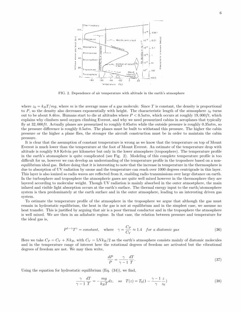
FIG. 2. Dependence of air temperature with altitude in the earth’s atmosphere
where z0 = kBT/mg, where m is the average mass of a gas molecule. Since T is constant, the density is proportionalto P , so the density also decreases exponentially with height. The characteristic length of the atmosphere z0 turnsout to be about 8.4km. Humans start to die at altitudes where P < 0.5atm, which occurs at roughly 19, 000ft, whichexplains why climbers need oxygen climbing Everest, and why we need pressurized cabins in aeroplanes that typicallyfly at 32, 000ft. Actually planes are pressurized to roughly 0.85atm while the outside pressure is roughly 0.35atm, sothe pressure difference is roughly 0.5atm. The planes must be built to withstand this pressure. The higher the cabinpressure or the higher a plane flies, the stronger the aircraft construction must be in order to maintain the cabinpressure.
It is clear that the assumption of constant temperature is wrong as we know that the temperature on top of MountEverest is much lower than the temperature at the foot of Mount Everest. An estimate of the temperature drop withaltitude is roughly 9.8 Kelvin per kilometer but only in the lower atmosphere (troposphere). The temperature profilein the earth’s atomosphere is quite complicated (see Fig. 2). Modeling of this complete temperature profile is toodifficult for us, however we can develop an understanding of the temperature profile in the troposhere based on a non-equilibrium ideal gas. Before doing that it is interesting to note that the increase in temperature in the thermosphere isdue to absorption of UV radiation by ozone and the temperature can reach over 1000 degrees centrigrade in this layer.This layer is also ionized so radio waves are reflected from it, enabling radio transmissions over large distance on earth.In the turbosphere and troposphere the atmospheric gases are quite well mixed however in the thermosphere they arelayered according to molecular weight. Though UV radiation is mainly absorbed in the outer atmostphere, the maininfared and visible light absorption occurs at the earth’s surface. The thermal energy input to the earth/atomospheresystem is then predominately at the earth surface and in the outer atmosphere, leading to an interesting driven gassystem.
To estimate the temperature profile of the atmosphere in the troposphere we argue that although the gas mustremain in hydrostatic equilibrium, the heat in the gas is not at equilibrium and in the simplest case, we assume noheat transfer. This is justified by arguing that air is a poor thermal conductor and in the troposphere the atmosphereis well mixed. We are then in an adiabatic regime. In that case, the relation between pressure and temperature forthe ideal gas is,
P 1−γT γ = constant, where γ =CPCV≈ 1.4 for a diatomic gas (36)
Here we take CP = CV +NkB , with CV = 5NkB/2 as the earth’s atmosphere consists mainly of diatomic moleculesand in the temperature range of interest here the rotational degrees of freedom are activated but the vibrationaldegrees of freedom are not. We may then write,
dP
P=
γ
γ − 1
dT
T. (37)
Using the equation for hydrostatic equilibrium (Eq. (34)), we find,
γ
γ − 1
dT
T= − mg
kBTdz, so T (z) = T0(1− γ − 1
γ
z
z0) (38)

7
Using Eq. (37) and the ideal gas law; ρ ∝ P/T , we also find,
P (z) = P0(1− γ − 1
γ
z
z0)γ/(γ−1); ρ(z) = ρ0(1− γ − 1
γ
z
z0)1/(γ−1) (39)
These equations lead to the prediction that the density of the atmosphere goes to zero at a critical thickness asopposed to a diffuse atmosphere as predicted by Eq. (35). Actually the exponential decay of the pressure leads to abehavior not too different than the power law of Eq. (39) as a = γ/(γ − 1) ≈ 3.5 is quite large. In fact in the limita→∞ we have,
(1− x
a)a → e−x (40)
so in that limit the adiabatic and isothermal pressure profiles are the same. Suprisingly the predictions of the adiabaticmodel are quite good for earth’s atmosphere for heights less than about z = 15km.
II. SPIN MODELS
The study of models for magnetic behavior have applications in all areas of physics and in many areas outsideof physics. The have played a key role in statistical physics, particularly in developing an understanding of phasetransitions. Ising in his PhD thesis showed that the one dimensional Ising magnet does not have a phase transitionat finite temperature while Onsager in a beautiful piece of work proved that the Ising model in two dimensions doeshave a phase transition. Ferromagnets are materials that exhibit spontaneous symmetry breaking and breaking ofergodicity where at low temperatures magnetization spontaneously appears without the application of an externalfield. In contrast paramagnets require an applied field in order to exhibit magnetization and at low field, h, themagnetization, m is proportional to the applied field. We first consider paramagnets.
1. Spin half and continuous spin paramagnets
We consider a case where the applied field lies along the easy axis of a magnet, so that the Hamiltonian is,
H = −µsh∑i
Si (41)
where µs is the magnetic moment of the system, h is the applied field and S = ±1 is the spin. The statisticalmechanics is easy to carry through as follows,
Z =
N∏i
(∑Si±1
eβµshSi) = 2NCoshN (βµsh) (42)
The magnetization is given by,
m =M
N=µsN
∑i
< Si >=1
N
∂(ln(Z))
∂(βh)= µstanh(βµsh) (43)
Other thermodynamic quantities of interest are the internal energy,
U = −∂ln(Z)
∂β= −Nµshtanh(βµsh) (44)
the Helmholtz energy and the entropy,
F = −kBT ln(Z) = −kBT ln(2cosh(βµsh)); S =1
T(U − F ) = NkB [ln(2cosh(βµsh))− βµshtanh(βµsh)] (45)
Surprisingly several important and general physical phenomena are contained in this model. The first two are relatedto the response functions, the magnetic susceptibility and the specific heat. The magnetic susceptibility,
χ =∂m
∂h= βµ2
ssech2(βµsh)→ µ2
s
kBT, as h→ 0. (46)
8
The behavior χ ∝ 1/T is called the Curie law and is used in experiments to see if the spins in the system areparamagnetic and to extract an effective value for the spin moment, µs, for the system. The specific heat of the modelis given by,
CV =
(∂U
∂T
)h
= NkB
(βµsh
cosh(βµsh)
)2
(47)
The specific heat approaches zero exponential at low temperatures and at high temperatures approaches zero as apower law ≈ 1/T 2. There is a peak in the specific heat at roughly kBTp ≈ level spacing/2 = µsh. Simple ideas aboutthe peak in the specific heat and entropy are used to interpret data such as that in Fig. 1 (left). The right figureshows the analogy between magnetic cooling and refridgeration using a gas cycle. Magnetic cooling is used to reducethe temperature below about 0.1K by using an intriguing property called negative temperature. This non-equilibriumproperty can be produced in our simple spin half paramagnetic system. The origin of the effect is seen by consideringthe entropy of the paramagnet as a function of its energy in the microcanonical ensemble with N,V,E as the controlvariables. If the number of up spins is n and the number of down is N −n, then the entropy and energy as a functionof the number of up spins is,
E = −µsh(n− (N − n)) = −µshN(2n
N− 1); S(E) = kBln
N !
n!(N − n)!= −kBN [ln(
n
N) + ln(1− n
N)] (48)
The entropy may be written in terms of the energy using,
n
N=
1
2− E
2µshN(49)
Of course the entropy is a maximum at n = N/2 where half of the spins are up and half are down. At this point theenergy is 0. The lowest energy state is where all spins are aligned with the field and at that point E = −µshN . As weincrease the energy from this value the entropy increases until we reach the highest entropy state at E = 0. However,and this is the key feature of this system, if the energy is raised further, the entropy decreases. Now consider the factthat the temperature is given by,
1
T=∂S
∂E(50)
so if the entropy increases with energy the temperature is positive and this is what happens at equilibrium. Howeverwhen we are away from equilibrium there is no need for the temperature to be positive. If we can prepare a statein a regime where the entropy decreases with energy, as in the paramagnetic model above, then the temperature isnegative. Clearly this is not a stable state so the system absorbs energy (heat) to return to a positive temperaturestate. This leads to the possibility of magnetic cooling where magnetic work is carried out to prepare the system ina state where the spins are aligned with a field. If the field is then switched off the system wants to return to thehigh entropy state at E = 0 and this leads to absorption of energy from the sample. This process is cycled to achievecooling (see figure 3). Mechanical work is done in polarizing the field and this work is used to produce refridgeration.
In many systems the spin is not restricted to the value 1/2 and instead we have combinations of spins (like in Fedue to Hund’s rule), which leads to many more possibilities. It is actually a good approximation in many cases toconsider the spin to be able to rotate to any angle on either the perimeter of a circle or on the surface of a sphere, sothat the field energy is given by,
H = −∑i
~µi · ~h (51)
where ~µi = µs~S and ~S is a vector with unit length that can lie on the surface of a sphere (Heisenberg model) or circle(XY model). We set the length of S to be one for convenience by absorbing the factor (S(S + 1))1/2 into µs. Themodel is still a non-interacting model so the canonical partition function is ZN1 , and for the (classical) continuousHeisenberg spin case,
Z1 =
∫sin(θ)dθdφeβµshcos(θ) =
4πsinh(βµsh)
βµsh(52)
The magnetization per spin is given by,
m =M
N=
∂
∂(βh)(ln(Z1)) = µs[coth(βµsh)− 1
βµsh] (53)

9
FIG. 3. left: Example of specific heat and entropy measurements of a magnetic system. Right: Comparison of magnetic coolingand cooling use a gas cycle (from Wikipedia)
For low fields (and sufficiently high temperatures) we find,
m ≈ µ2s
3kBTh; so χ =
∂m
∂h=
µ2s
3kBT(54)
For both the spin half and continuous spin cases we find the Curie law which is characteristic of “classical” param-agnets. As we shall see when we study the Fermi gas, a very different behavior occurs when the gas has quantumdegeneracy.
2. Spin half nearest neighbor Ising model in one dimension and two dimensions
A key question in statistical physics is whether a system is capable of having a phase transition. The Ising model isa comparatively simple system where we can address this question with some precision. The first question is whethera one dimensional Ising model has a phase transition at finite temperature and this can be answered by solving theproblem exactly. First however we go through a simple argument due to Peierls that shows a finite temperature phasetransition is not possible for the one-dimensional spin-half Ising model with nearest-neighor interactions.
The one-dimensional nearest neighbor Ising model has Hamiltonian,
H = −JN∑i=1
SiSi+1 (55)
where Si = ±1. The Peierls argument considers the stability of the ground state (all up spins) to topological excitationswhere in this problem the excitations are domains of the opposite orientation. In a problem with free boundaries wecan consider a simpler problem consisting of a single “domain wall” between a region of all up spins and a region ofall down spins. If the free energy of this excitation is lower than the ground state, then the ground state is unstable.The difference in Helmholz free energy between a system with a domain wall and that without a domain wall is givenby,
δF = δU − TδS = 4J − kBT ln(N) (56)
where we consider a fixed temperature. Since δF < 0 for finite T provided N is sufficiently large, the one dimensionalIsing ground state is unstable to long wavelength fluctuations. It therefore cannot have a phase transition at finitetemperature.
Now we solve the problem exactly and check if the Peierls argument is right. We use periodic boundary conditionsso the model is defined on a ring. It is useful to solve this problem using transfer matrices as they can be generalizedto many problems and provide a method for tranforming a classical problem at finite temperature into the groundstate of a quantum problem in one lower dimensions. The transfer matrix for the one dimensional Ising model is atwo by two matrix, with matrix elements,
TS,S′ = eβJSS′
(57)

10
where S, S′ take values ±1 as usual. The partition function may then be written as,
Z =∑S1
∑S2
....∑SN
eβJ∑
iSiSi+1 =
∑S1
∑S2
....∑SN
< S1|T |S2 >< S2|T |S3 > .... < SN |T |S1 > (58)
This reduces to,
Z = tr(TN ) = λN1 + λN2 (59)
where λ1,2 are the eigenvalues of the transfer matrix T . The problem is then reduced to diagonalizing a two by twomatrix. We find that the eigenvalues of the transfer matrix are,
λ1 = 2Cosh(βJ); λ2 = 2Sinh(βJ) (60)
so that,
Z = 2N [CoshN (βJ) + SinhN (βJ)] (61)
The specific heat can be calculated by using,
F = −kBT ln(Z) = −kBTN [ln(2) + ln(Cosh(βJ)] (62)
so that,
CV = T∂2F
∂T 2= NkB(
J
kBT)2sech2(
J
kBT) (63)
At low temperatures this reduces to,
CVNkB
≈ (J
kBT)2Exp[− 2J
kBT] as T → 0 (64)
while
CVNkB
≈ (J
kBT)2 as T →∞ (65)
The specific heat thus approaches zero exponentially at low temperatures and approaches zero algebraically at hightemperatures. There is a peak in the specific heat at around J = kBT . This is typical of systems that have a “gap”of order J between the ground state and the first excited state.
Solution of the two dimensional Ising model is carried out using the transfer matrix method, however the transfermatrix is of dimension 2L × 2L where L is the transverse dimension of the square lattice strip. In a spectacularcalculation, Onsager found the exact solution and from it found the following results (1944),
(βJ)c =1
2ln(1 +
√2) or (
kBT
J)c ≈ 2.2691... (66)
and near the critical point the specific heat behaves as, for T < Tc,
CVNkB
≈ 2
π(
2J
kBTC)2[−ln(1− T
Tc) + ln(
kBT
2J)− (1 +
π
4)] (67)
The specific heat thus diverges logarithmically on approach to Tc. The low and high temperature behavior is similarto that in the one dimensional case.
The magnetization can also be calculated. In the one dimensional case the transfer matrix can be extended to treatthe hamiltonian,
H = −J∑i
SiSi+1 − h∑i
Si (68)
The magnetization is found from ∂ln(Z)/∂(h), leading to,
m(h, T ) =Sinh(βh)
[Sinh2(βh) + e−4βJ ]1/2; 1d Ising. (69)

11
From this expression it is seen that the magnetization is zero for h = 0 in one dimension.In two dimensions an exact result in finite field has not been found, but the magnetization in zero field has been
found, with the result that for T < Tc with h = 0,
m(h = 0, T ) =(1− [Sinh(2βJ)]−4
)1/82d Ising, T < Tc (70)
Near the critical point this reduces to,
m(h = 0, T ) ∝ (Tc − T )1/8 T < Tc, h = 0 (71)
The critical exponent for the Ising order parameter is thus 1/8 in two dimensions however this exponent depends onthe spational dimension and is 1/2 above the so-called ”upper critical dimension”. There is no phase transition inone dimension. What is the behavior in three dimensions?? We shall return to the general issue of phase transitionsand critical exponents in Part 3 of the course. Now we show that the behavior above the upper critical dimension isfound using mean field theory. In fact, as we shall explore further in Part 3 of the course, systems in high dimensionsor with long range interactions are usually well described by mean field theory.
3. Infinite range model of an Ising ferromagnet
The Ising model is very difficult, even in two dimensions where there is an exact solution. However the infiniterange model is relatively easy to solve and exhibits an interesting phase transition. The infinite range model is oftenthe same as a mean field model, as is the case for the Ising ferromagnet. Mean field theory in its many forms, andwith many different names, is the most important first approach to solving complex interacting many body problems.The Hamiltonian for the infinite range model is,
H = − JN
∑SiSj (72)
so the partition function is,
Z = (
N∏i
∑Si±1
)eβ JN
∑ijSiSj = (
N∏i
∑Si±1
)eβJN (∑
iSi)
2
(73)
Using the Gaussian integral, ∫ ∞−∞
e−x2+bxdx =
√π√aeb
2/4a (74)
we write,
Z =
∫ ∞−∞
dx√πe−x
2N∏i
(∑Si±1
e2x(β JN )1/2Si) (75)
Doing the sums gives,
Z =
∫ ∞−∞
dx√πe−x
2
2N [Cosh(2x(βJ
N)1/2)]N (76)
We write this in the form,
Z =
∫ ∞−∞
dx√πef(x); where, f(x) = −x2 +N [ln(2) + ln(Cosh(2x(β
J
N)1/2)] (77)
Since f(x) contains a large parameter N , it is a sharply peaked function, so we can use the method of steepestdescents. This method states that if the function f(x) has a set of maxima, then the integral is dominated by thelargest of these maxima, in the thermodynamic limit. At the dominant maximum, xmax, the first derivative is zero,so the expansion to quadratic order is,
f(x) = f(xmax)− (x− xmax)2
2!|f′′(xmax)|+ ... (78)
12
where f ′′(xmax) < 0 as we are at a maximum. Using this expansion in the integral we find,∫ef(x)dx→ ef(xmax)
∫ ∞−∞
e−(x−xxmax)2
2! f′′
(xmax)dx =
(2π
|f ′′(xmax)|
)1/2
ef(xmax). (79)
The problem then reduces to finding the maxima of the function f(x), or the minima of the function −f(x). To findthe maxima in the case of the Ising model, we take a derivative with respect to x of f(x) in Eq. (77), that leads to,
x = N(βJ
N)1/2tanh(2
βJ
N)1/2x (80)
We define, y = 2(βJ/N)1/2x to find,
y = 2βJtanh(y) (81)
For small values of βJ < (βJ)c, the only solution to this equation is at y = 0, so in that case,
Z →(
π
|f ′′(xmax)|
)1/21√πeNln(2) (82)
The Helmholtz free energy is, F = −kBTNln(2), where we drop the prefactor terms that are much lower order. Forlarge values of βJ > (βJ)c, there are three solutions. The behavior in this regime can be treated analytically byexpanding to cubic order in y, so that,
y = 2βJ(y − 1
3y3) (83)
this has three solutions,
y = 0; y = ±[3(2βJ − 1)]1/2 (84)
When 2βJ > 1, the second pair of solutions is real, while when 2βJ < 1 they are imaginary. The critical point isthen at (βJ)c = 1
2 , and the behavior near the critical point is y ≈ [6(βJ − (βJ)c)]1/2.
Integration of Eq. (83) or a fourth order expansion of (77) leads to,
−fR(y) ≈ a1(T − Tc)y2 + a2y4, (85)
where a1 and a2 are positive and constant terms along with higher order terms in y have been dropped. This expressionis the same as the Landau free energy for an Ising system, as we shall see in the next section of the course. Thefunction f(y) is a reduced free energy. We then intepret y as the order parameter for the Ising model, so that y ∝ m,and we find that the order parameter approaches zero as m ∝ (Tc − T )1/2 which is typical mean field behavior.
The exact solutions above enable us to state some very interesting properties of the Ising model that provide abasis for a more general discussion of phase transitions as a function of dimension and range of interaction. For adiscussion of critical behavior we focus only on the magnetization, that behaves as
m ≈ (Tc − T )βI T → Tc from below. (86)
We have the following results for the Ising model with short range interactions:- In one dimension there is no phase transition at finite temperature.- In two dimensions there is a phase transition at finite temperature, βI = 1/8.- In a long range model there is phase transition at finite temperature, βI = 1/2.These results are consistent with some general postulates about phase transitions that we shall return to in Parts
2 and 3 of the course:1. Below a lower critical dimension, dlc, fluctuations destroy the ordered state at any finite temperature. For the
Ising model dlc = 1 + δ.2. Above an upper critical dimension, duc, the critical behavior is given by mean field theory, which in turn is
equivalent to the behavior of a model with infinite range interactions. For the ferromagnetic Ising model treatedabove, βI = 1/2 in all of these cases.
3. Between the lower and upper critical dimensions the critical behavior is dependent on the spatial dimension. Inthe case of the short range ferromagnetic Ising model the critical exponent β changes with dimensions and the uppercritical dimension is 4.
13
III. STATISTICAL PHYSICS BY FILLING SINGLE PARTICLE ENERGY LEVELSAPPLICATIONS TO QUANTUM AND CLASSICAL GASES
A. Statistics of filling energy levels for Bose, Fermi and Classical gases
A great deal of theoretical physics reduces complex many body problems to single particle problems and in quantumproblems this reduces to filling up single particle energy levels. A many body state is then a configuration ofoccupancies of the single particle energy levels and the statistical physics is based on methods to calculate thethermodynamics for different energy levels and different methods for filling these energy levels. We consider threeways of filling a set of single particle energy levels, ε1...εM . We also include the possibility that these single particleenergy levels each has its own degeneracy, so the energy levels are characterized by εi, gi, where gi is the degneracyof energy level i.
We consider three ways of filling these energy levels: Fermi statistics, Bose statistics and Maxwell-Boltzmannstatistics. We concentrate on the grand canonical partition function that reduces to a product of single energy levelgrand partition functions and for the Bose or Fermi cases, we have,
ΞB,F =∏i
(∑ni
e(−βεi+βµ)ni
)gi=∏i
(Ξi)gi (87)
Our task is now reduced to filling a single energy level in the correct manner for the cases of Bose, Fermi statisticsin order to calculate Ξi In the Bose and Fermi cases we have to fill energy levels in ways that are consistent with themany particle wavefunctions that are constructed for each configuration.
For example, for a two particle Fermi system we construct a wavefunction by placing two fermions in different singleparticle states. The correct antisymmetric state is given by,
1
21/2(φi(x1)φj(x2)− φi(x2)φj(x1)) (88)
The only way that a correctly antisymmetrized two particle state can be constructed from single particle wavefunctionsis to omit any configurations where two fermions are in the same single particle state, because if we set i = jin the expression above we get zero which means we cannot construct a wavefunction for that case. In generalantisymmetrized wave functions constructed from single particle states may be found by forming a determinant,called a Slater determinant, which is of the form,
Ψ(x1,x2, . . . ,xN ) =1√N !
∣∣∣∣∣∣∣∣∣ψ1(x1) ψ2(x1) · · · ψN (x1)ψ1(x2) ψ2(x2) · · · ψN (x2)
......
...ψ1(xN ) ψ2(xN ) · · · ψN (xN )
∣∣∣∣∣∣∣∣∣ . (89)
This determinant captures the fact that if any pair of the single particle wavefunctions used in the construction of thedeterminant are the same, then the determinant is zero so two particles can never be in the same single particle state.it This means that for fermions we must restrict the filling of single particle energy levels so that there is only onefermion or no fermions in any energy level. Of course if there are additional quantum numbers such as spin, color orisospin, an energy level also has a specific value for each of these quantities. In the case of spin for example we wouldassign a degeneracy of gi = 2 to account for the two possible spin orientations. Particles with different spin or otherquantum number are considered to be different particles, so it is possible to put an up spin fermion and a down spinfermion in the same spatial wavefuntion. The spin wavefunction then provides the distinction between the states anda correct antisymmetrized product wavefunction (product of spatial and spin parts) can be constructed.
In the Bose case we have to construct wavefunctions that are symmetric under exchange. For this reason we canconstruct wavefunctions with many particles in one energy level, so for example,
φi(x1)φi(x2) (90)
is a good wavefuntion for two bosons. This can be generalized to any number of wavefunctions so we can put anynumber of Boson particles in a single particle energy level. To construct a Boson state using different single particlestates, we have to add all possible combinations which turns out to the the same structure as a determinant, but withall the signs in the expansion of a determinant changed to positive. This is called a Permanent. Though evaluationof a permanent seems easier than evaluating a determinant, it is not. The reason is that a determinant is equal

14
to the product of the eigenvalues, while the permanent does not have a simple expression in terms of eigenvaluesand cannot be reduced using linear transformations. The determinant has the nice property that Det(ABC) =Det(A)Det(B)Det(C), so the determinant is invariant under non-singular similarity transformations. The permanentdoes not have this property so we are stuck with a minor expansion which is of order N ! where N is the dimensionof the single particle basis. This is much worse that diagonalizing a matrix which is at most N3. In computationalterms evaluating the permanent is in general NP-hard while evaluating the determinant in polynomial.
Now that we know how to fill the single particle energy levels we can write down explicit expressions for the singleenergy level grand partition functions Ξi. For the fermi case we have,
ΞFi =∑ni=0,1
e−β(εi−µ)ni = 1 + e−β(εi−µ) = 1 + ze−βεi . (91)
The Bose case is,
ΞBi =∑
ni=0,1...∞e−β(εi−µ)ni =
1
1− e−β(εi−µ)=
1
1− ze−βεi. (92)
For the Maxwell-Boltzmann (classical) case we can have any number of particles in each energy level, provided weinclude the Gibbs factor so that,
ΞMBi =
∑ni=0,1..∞
1
ni!e−β(εi−µ)ni = Exp[e−β(εi−µ)] = Exp[ze−βεi ] (93)
The thermodynamic properties are found using,
φG = −PV = −kBT ln(Ξ) = −kBT ln(∏i
(Ξi)gi = −kBT
∑i
giln(Ξi) (94)
From this expression we can find the thermodynamics for any of the gases, using,
dφG = −SdT − PdV −Ndµ (95)
Further relations that we will use frequently are,
< ni >= − 1
β
∂ln(Ξ)
∂εi; N =
∑i
< ni >; U =∑i
εi < ni >= −(∂ln(Ξ)
∂β)z. (96)
Carrying out the derivatives we find,
< ni >B=gize
−βεi
1− ze−βεi; < ni >F=
gize−βεi
1 + ze−βεi. (97)
where z = eβµ is the fugacity. < ni > is the occupancy of all gi degenerate levels with energy εi. Remove the factorof gi to find the average occupancy of any one of the degenerate states. These expressions are often summarized as,
< n >±=1
eβ(ε−µ) ± 1(98)
which is the occupancy of any one non-degenerate energy level with energy ε and the plus(minus) sign refers tofermions (bosons).
B. Energy levels for a particle in a box
To proceed further we need the energy levels and in this course most of the calculations are for ideal gases wherethe energy levels are those of a particle in a box that are given by,
ε~k =h2~k2
2m, non− relativistic, (99)
ε~k = hkc, ultra− relativistic (100)
15
and
ε~k =√
(hkc)2 + (m0c2)2, general (101)
In each case the wavefunction in the box is a standing wave that must have zero amplitude at the edges of the box.If we take the box to be a hypercube, each dimension can be treated independently and if we take the interior of thebox to lie on the interval 0 < x < L for each direction, then choosing sinusoidal wave functions that for the threedimensional case is,
ψ = Asin(kxx)sin(kyy)sin(kzz). (102)
Then for each co-ordinate we must have,
sin(klL) = 0; so kl =π
Lsl (103)
where nl is a positive integer. For arbitrary dimensions we then find,
~k =π
L(s1, s2, ...sd) (104)
with nl positive integers and d the spatial dimension.To calculate ensemble averages, we need to carry out a sum over all of the energy levels. To do this it is usually
convenient to convert the sum to an integral, for example in three dimensions,
∑sx,sy,sz
→(L
π
)3 ∫ ∞0
d3k + T0 =
(L
2π
)3 ∫ ∞−∞
d3k + T0 =
(L
2π
)3 ∫ ∞0
4πk2dk + T0 (105)
Where the last integral form applies to energy levels that for only depend on the modulus of k = |~k|. The term T0 isneeded in cases of Bose condensation where the ground state occupancy has to be treated separately from the excitedstates.
C. Photon gas thermodynamics
One of the the most remarkable predictions of quantum statistical physics is the Planck blackbody spectrum. Tofind the blackbody spectrum and to analyse the thermodynamics of photons gas, we consider energy-momentumdispersion relation εp = pc = hkc = hω = hν = hc/λ, i.e. the ultrarelativistic case. We set the chemical potential tozero as there can be an infinity of photons at zero energy. Actually the chemical potential of photons is not alwayszero as there are cases in photochemistry and photovoltaics where photons have a chemical potential that is less thanzero. However for the case of photons in a box, i.e. blackbody radiation, the chemical potential is zero. We areactually treating the Bose condensed phase of the photon gas. However we are only interested in the excited statepart of the system.
Defining p = hk and using z = 1 and equations (96), (97), (100) and (105) we find for the three dimensional idealphoton gas,
ln(Ξ) = −2
(L
2πh
)3 ∫ ∞0
4πp2dp ln(1− e−βpc), (106)
while the number of excited state photons is,
N = 2
(L
2πh
)3 ∫ ∞0
4πp2dpe−βpc
1− e−βpc= V
∫dω n(ω) (107)
and the internal energy is given by,
U = 2
(L
2πh
)3 ∫ ∞0
4πp2dp (pc)e−βpc
1− e−βpc= V
∫dω u(ω) (108)
where n(ω) is the number density of photons and u(ω) is the energy density at angular frequency ω. Notice thatthe T0 term has been dropped as it does not contribute to the physics of the ideal photon gas (that we know of).

16
FIG. 4. Comparison of the blackbody photon spectral intensity (Eq. (109) below) with experiments: Left figure: The cosmicmicrowave background measured by the COBE satellite; Right figure: The solar intensity outside the atmosphere and at theearth’s surface.
The additional factor gi = 2 in front of these equations is due to the two polarizations that are possible for photons.These functions characterize the “blackbody spectrum” inside the box confining the photon gas, with temperatureT . However measurements of radiation measure radiation spectral intensity, which is related to the energy densityby the relation, i(ω) = u(ω)c. Moreover, the Planck radiation law is often quoted in a slightly different way. It isoften defined to be the radiant spectral intensity per unit solid angle, which is related to the spectral energy densityby u(ω) by is(ω, T ) = c u(ω)/(4π), where 4π is solid angle of a sphere. Several forms of is are common, including:
is(ω, T ) =h
4π3c2ω3
eβhω − 1or is(ν, T ) =
2h
c2ν3
eβhν − 1; or is(ν, T ) =
2c2h
λ5
1
eβhc/λ − 1(109)
Blackbody spectra provide a surprisingly good description of many systems (see Figure 4), including the cosmicmicrowave background, with temperature TCMB = 2.713K; and the spectral intensity reaching earth from stars suchas our Sun with T = 5500K, Antares with T = 3400K, Spica with T = 23, 000K.
The average properties of the photon gas is found by integration, using the integral,∫ ∞0
xs−1dx
ex − 1= Γ(s)ζ(s), (110)
where Γ(s) = (s− 1)! for s a positive integer , and ζ(3) = 1.202..., ζ(4) = π4/90. For s = 4, we find γ(s)ζ(s) = π4/15.
U
V=
π2k4B
15h3c3T 4; PV =
1
3U ; N = V
2ζ(3)(kBT )3
π2h3c3(111)
Two other nice relations for the photon gas that can be derived from standard thermodynamic relations are S =4U/(3T ), CV = 3S.
The Stefan-Boltzmann law ISB = σT 4, is the power per unit area radiated from a blackbody with emissivity one.The relation ISB and U/V of the photon gas is, are as follows,
ISB(T ) =c
4
U
V= σSBT
4; where σSB =π2k4
B
60h3c2(112)
where σSB is the Stefan Boltzmann constant. The factor c/4 has two orgins, the first factor (c) comes from therelationship between the energy of a travelling wave and its intensity, and the second is a geometric factor due to anassumption of isotropic emission from a small surface element on the surface of the emitter. To understand the firstfactor, consider a classical EM wave in free space with energy density u = ε0E
20/2 + B2
0/(2µ0). In the direction ofpropagation of the wave, the energy crossing a surface of area A per unit time is,
Energy per unit time = Power = u ∗A ∗ c so that Iw = Power/Area = uc (113)
where Iw is the intensity of the wave. This applies to both the peak and rms intensity of the wave, provided theenergy density is the peak or rms value respectively. The geometric factor comes from considering a small flat surface
17
element that emits radiation in all directions. In the case of blackbody radiation, this element is considered to be atthe surface, so it emits half of its radiation back into the black body and half out of the black body. In addition, theradiation in the direction normal to the surface is reduced from the total radiation emitted from the surface elementdue to the assumption of isotropic emission. The component normal to the surface is found by finding the componentof the electric field in the formal direction, E0cos(θ), then squaring this to get the correct projection of the intensity,and then averaging over angles θ in a hemisphere. The result is that we need to average cos2(θ) over a half period.This leads to a geometric factor of 1/2. Multiplying these two factors of 1/2 gives the total geometric factor of 1/4.In most applications, the Stefan-Boltzmann law needs to be modified to account for the emissivity of the material(e) and the geometry of the surface and the location of the observer with respect to the surface, if the surface is notspherical.
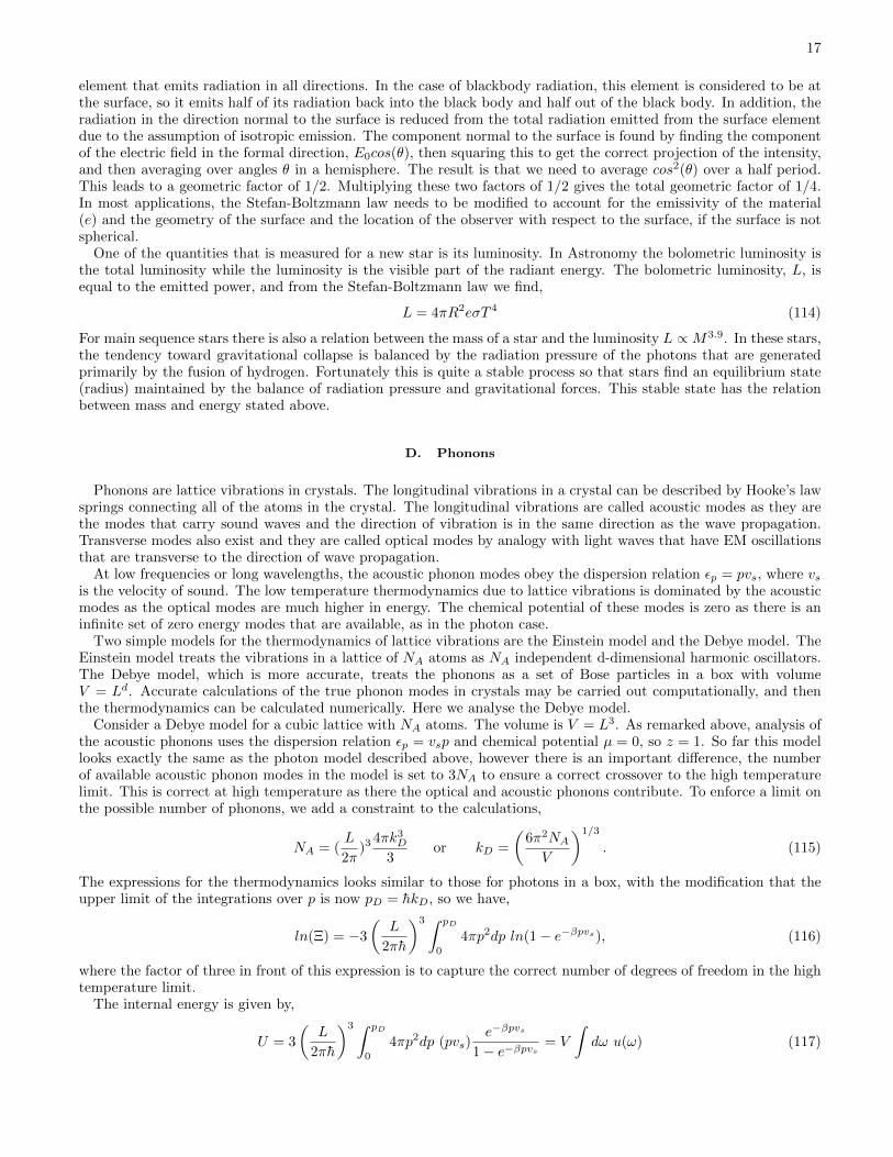
One of the quantities that is measured for a new star is its luminosity. In Astronomy the bolometric luminosity isthe total luminosity while the luminosity is the visible part of the radiant energy. The bolometric luminosity, L, isequal to the emitted power, and from the Stefan-Boltzmann law we find,
L = 4πR2eσT 4 (114)
For main sequence stars there is also a relation between the mass of a star and the luminosity L ∝M3.9. In these stars,the tendency toward gravitational collapse is balanced by the radiation pressure of the photons that are generatedprimarily by the fusion of hydrogen. Fortunately this is quite a stable process so that stars find an equilibrium state(radius) maintained by the balance of radiation pressure and gravitational forces. This stable state has the relationbetween mass and energy stated above.
D. Phonons
Phonons are lattice vibrations in crystals. The longitudinal vibrations in a crystal can be described by Hooke’s lawsprings connecting all of the atoms in the crystal. The longitudinal vibrations are called acoustic modes as they arethe modes that carry sound waves and the direction of vibration is in the same direction as the wave propagation.Transverse modes also exist and they are called optical modes by analogy with light waves that have EM oscillationsthat are transverse to the direction of wave propagation.
At low frequencies or long wavelengths, the acoustic phonon modes obey the dispersion relation εp = pvs, where vsis the velocity of sound. The low temperature thermodynamics due to lattice vibrations is dominated by the acousticmodes as the optical modes are much higher in energy. The chemical potential of these modes is zero as there is aninfinite set of zero energy modes that are available, as in the photon case.
Two simple models for the thermodynamics of lattice vibrations are the Einstein model and the Debye model. TheEinstein model treats the vibrations in a lattice of NA atoms as NA independent d-dimensional harmonic oscillators.The Debye model, which is more accurate, treats the phonons as a set of Bose particles in a box with volumeV = Ld. Accurate calculations of the true phonon modes in crystals may be carried out computationally, and thenthe thermodynamics can be calculated numerically. Here we analyse the Debye model.
Consider a Debye model for a cubic lattice with NA atoms. The volume is V = L3. As remarked above, analysis ofthe acoustic phonons uses the dispersion relation εp = vsp and chemical potential µ = 0, so z = 1. So far this modellooks exactly the same as the photon model described above, however there is an important difference, the numberof available acoustic phonon modes in the model is set to 3NA to ensure a correct crossover to the high temperaturelimit. This is correct at high temperature as there the optical and acoustic phonons contribute. To enforce a limit onthe possible number of phonons, we add a constraint to the calculations,
NA = (L
2π)3 4πk3
D
3or kD =
(6π2NAV
)1/3
. (115)
The expressions for the thermodynamics looks similar to those for photons in a box, with the modification that theupper limit of the integrations over p is now pD = hkD, so we have,
ln(Ξ) = −3
(L
2πh
)3 ∫ pD
0
4πp2dp ln(1− e−βpvs), (116)
where the factor of three in front of this expression is to capture the correct number of degrees of freedom in the hightemperature limit.
The internal energy is given by,
U = 3
(L
2πh
)3 ∫ pD
0
4πp2dp (pvs)e−βpvs
1− e−βpvs= V
∫dω u(ω) (117)
18
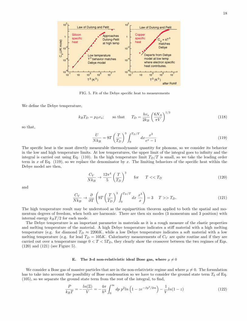
FIG. 5. Fit of the Debye specific heat to measurements
We define the Debye temperature,
kBTD = pDvs; so that TD =hvs2kB
(6NAπV
)1/3
(118)
so that,
U
NkB= 9T
(T
TD
)3 ∫ TD/T
0
dxx3
ex − 1(119)
The specific heat is the most directly measurable thermodynamic quantity for phonons, so we consider its behaviorin the low and high temperature limits. At low temperatures, the upper limit of the integral goes to infinity and theintegral is carried out using Eq. (110). In the high temperature limit TD/T is small, so we take the leading orderterm in x of Eq. (119), so we replace the denominator by x. The limiting behaviors of the specific heat within theDebye model are then,
CVNkB
→ 12π4
5
(T
TD
)3
for T << TD (120)
and
CVNkB
→ ∂
∂T
(9T
(T
TD
)3 ∫ TD/T
0
dxx3
x
)= 3 T >> TD. (121)
The high temperature result may be understood as the equipartition theorem applied to both the spatial and mo-mentum degrees of freedom, when both are harmonic. There are then six modes (3 momentum and 3 position) withinternal energy kBT/2 for each mode.
The Debye temperature is an important parameter in materials as it is a rough measure of the elastic propertiesand melting temperature of the material. A high Debye temperature indicates a stiff material with a high meltingtemperature (e.g. for diamond TD ≈ 2200K, while a low Debye temperature indicates a soft material with a lowmelting temperature (e.g. for lead TD = 105K. Calorimetry measurements of CV are quite routine and if they arecarried out over a temperature range 0 < T < 5TD, they clearly show the crossover between the two regimes of Eqs.(120) and (121) (see Figure 5).
E. The 3-d non-relativistic ideal Bose gas, where µ 6= 0
We consider a Bose gas of massive particles that are in the non-relativistic regime and where µ 6= 0. The formulationhas to take into account the possibility of Bose condensation so we have to consider the ground state term T0 of Eq.(105), so we separate the ground state term from the rest of the integral, to find,
P
kBT= − ln(Ξ)
V= −4π
h3
∫ ∞0
dp p2ln(
1− ze−βp2/2m
)− 1
Vln(1− z) (122)
19
As we shall show later the ground state term in this expression can be ignored, so henceforth we neglect in. Howeverthe ground state term in the number of Bosons, so we consider,
N
V=
4π
h3
∫ ∞0
dp p2 ze−βp2/2m
1− ze−βp2/2m+
1
V
z
1− z(123)
and the internal energy is given by,
U
V=
4π
h3
∫ ∞0
dp p2 p2
2m
ze−βp2/2m
1− ze−βp2/2m. (124)
In the expression for U , we dropped the ground state term, T0, as the p2/2m term in the sum goes to zero sufficientlyquickly as p → 0 that the ground state contribution can no longer be singular. As we shall see later when we treatBose condensation, the ln(1− z) term in the expression for the pressure may also be dropped. However the z/(1− z)term in the total number of particles is not negligible and provides the description of the Bose condensed fraction ofthe gas. Using integration by parts it is straightforward to show that,
P =2
3
U
V. (125)
For dispersion relations of the form εk = cks, in d dimensions this generalizes to the same expression as applies to theBose gas, ie. P = su/d.
Using the change of variables x2 = βp2/2m, we find
P = −kBTλ3
4
π1/2
∫ ∞0
dx x2ln(1− ze−x2
);N
V=
1
λ3
8
π1/2
∫ ∞0
dx x3 ze−x2
1− ze−x2 +1
V
z
1− z(126)
The thermodynamic functions are most succintly stated in terms of the functions g3/2(z) and g5/2(z) so that Eqs.(126) reduce to,
P =kBT
λ3g5/2(z);
N
V=
1
λ3g3/2(z) +
1
V
z
1− z(127)
where,
g5/2(z) = − 4
π1/2
∫dx x2ln(1− ze−x
2
) =
∞∑l=1
zl
l5/2; g3/2(z) = z
∂
∂zg5/2(z) =
∞∑l=1
zl
l3/2. (128)
The series expansion for g5/2 is found by expanding the logarithm in the integral form of g5/2 and then integratingthe Gaussians that remain, using,
ln(1− y) = −∞∑l=1
zl
l;
∫ ∞0
dx x2e−lx2
=π1/2
4
1
l3/2. (129)
The expansion for g3/2 can be found by differention or by expanding 1/(1−y) and carrying out the Gaussian integrals.
F. High temperature limit - the classical ideal gas
First we look at the behavior at high temperatures where we expect to recover the classical, Maxwell-Boltzmanngas. In the high temperature limit, z = e−βµ is small because the chemical potential is large and negative, so we canexpand in z to find,
N
V=
1
λ3g3/2(z) =
1
λ3(z +
z2
23/2+ ..) (130)
Keeping only the leading order term in the expansion on the right hand side of this equation we find
z =Nλ3
V; and using βµ = ln(z); (131)
20
we find the chemical potential of the Bose gas in the high temperature limit is,
µ = kBT ln(Nλ3
V) (132)
which is the same as the chemical potential found in the classical ideal gas (see Eq. (15)) of the lecture notes for Part2. Note that the chemical potential is large and negative at high temperature, so the fugacity approaches zero. Thefugacity is always positive as it is an exponential of real number.
From Eq. (52) using the leading order g5/2 = z, along with z = Nλ3/V as found above, give the ideal gas law andthe equipartition result for the internal energy of the classical ideal gas. Problem 4 of the assignment asks that youcalculate the next correction to the classical limit. This is achieved by considering the next term in the expansion ofEq. (130).
G. Low temperature limit and Bose Einstein Condensation (BEC)
Now we consider the low temperature limit where BEC can occur. Bose condensation is a very important phenomenathat is closely related to superfluidity, superconductivity and other phase coherent phenomena such as lasing. Howeverthe Bose condensation of gases has been very difficult to achieve. In most cases Bose condensation occurs in systemsmade up of composite Bosons, such as Helium 4 in superfluidity and cooper pairs in superconductivity. CompositeBosons consist of an even number of Fermions that may be of different types, for example in Helium 4, 2 protons, 2neutrons and 2 electrons. The hydrogen atom itself can form a composite Boson (one proton and one electron) andany system where the spin adds to an integer is has this possibility. For this reason Wolfgang Ketterle’s group focusedon achieving Bose Condensation in atomic Hydrogen gases in atom traps. However Bose condensation can only occurif other phase transitions and/or bonding interactions are avoided. In the case of Hydrogen for example formationof Hydrogen molecules and then a hydrogen solid at temperatures around 14K prevent formation of the BEC state.Attempts to form a BEC state in Alkali metal gases were finally successful in 1995 when a group at U. Colorado(Wieman and Cornell) with the observation of BEC in Rubidium 85 at 170 nano Kelvin. This lead to the nobel prizein physics for BEC in 2001 (Cornell, Wieman, Ketterle). Though high densities favor condensation, competing statesare also favored so the gases need to be kept quite dilute to allow BEC to occur. The number of atoms involved in thecondensates was originally only about 10,000 atoms, though that number has risen significantly since. Though a fulldescription of BEC in atom traps requires treatment of the trap potential, particle-particle scattering and finite sizeeffects, the ideal gas BEC is the starting point about which the more complex effects can be treated perturbatively.Here we concentrate on the ideal gas case.
As noted above, the chemical potential of gases are large and negative at high temperature, so the fugacity ap-proaches zero as T →∞. At low temperatures, the chemical potential is dominated by the energy contribution. For aBose system where the ground state energy is at zero energy, the change in energy on addition of a particle is zero, sothe chemical potential approaches zero as T → 0. In the Bose case, the equation for the number density of particlesconsists of a ground state part and a finite temperature part,
N =V
λ3g3/2(z) +
z
1− z= N1 +N0 (133)
where N1 is the number of Bose particles in the excited states and N0 is the number of Bose particles in the groundstate. As noted above, the largest value that z can take for a Bose gas is z = 1, therefore the largest possible valuethat N1 can take is,
Nmax1 =
V
λ3g3/2(1) =
V
λ3ζ(3/2) (134)
where ζ(x) is the Reimann zeta function ζ(z) =∑l−z and ζ(3/2) = 2.612.... Bose condensation occurs when
Nmax1 < N as if this occurs, the remaining Bose particles must be in the ground state. Therefore the condition for
Bose condensation is,
N = Nmax1 = ζ(3/2)
V
λ3c
; orNλ3
V=
Nh3
V (2πmkBTc)3/2= ζ(3/2) (135)
or,
Tc =h2
2πmkB
(N
V ζ(3/2)
)2/3
. (136)

21
FIG. 6. Left: Phase space density of Strontium atoms released from trap (IQOQI group Austria). Right: Chromium 52 trappedatomic gas condensate fraction as a function of temperature (triangles) compared to the ideal Bose gas (solid). Deviationspredicted by theory (solid dots) are due to finite number of atoms and due to interactions (from Pfau group www page at U.Stuttgart).
From this we see that BEC is favored for high density gases consisting of particles with low mass, provided otherinteractions can be prevented from interfering with the BEC. In alkali metals in gases it turns out the heavier particlesare easier to condense despite the fact that their mass is higher.
Using the mass and density of Helium 4 the above equation gives Tc = 3.13K. The superfluid transition in Helium4 is actually at Tc = 2.18K so the BEC theory is not very good for Helium 4, but that is not surprising as Helium 4is not an ideal gas. However for atom traps the ideal Bose gas BEC transition is a much better model (see Fig. 6).Because µ = 0 and hence z = 1 in the Bose condensed state, the thermodynamics can be calculated in terms of ζfunctions, for example the fraction of the Bose gas that is in the condensed phase is,
fs =N0
N= 1− N1
N= 1− V
Nλ3ζ(3/2) = 1−
(T
Tc
)3/2
T ≤ Tc. (137)
where fs is the condensed or superfluid fraction of the gas. The internal energy is given by,
U
V=
3
2
kBT
λ3g5/2(1) =
3
2
kB(2πmkB)3/2
h3T 5/2g5/2(1) =
3
2
N
VkBT
(T
Tc
)3/2 g5/2(1)
g3/2(1)T ≤ Tc (138)
The specific heat at constant volume is then (using ζ(5/2) = 1.3415,
CV =15
4
kB(2πmkB)3/2
h3T 3/2g5/2(1) =
15
4NkB
(T
Tc
)3/2 g5/2(1)
g3/2(1)(139)
The specific heat then goes to zero as T → 0. The peak value of the specific heat is at T = Tc, where it takes thevalue
CV (Tc) =15
4NkB
g5/2(1)
g3/2(1)≈ 1.926NkB (140)
This can be compared to the ideal gas result Cv = 1.5NkB (Dulong-Petit law), which is correct at high temperature.There is a cusp in the specific heat at T = Tc due to the Bose condensation phase transition. This cusp behavioris quite different that that observed in Helium 4 (the λ transition) where there is a much sharper divergence atthe transition, so the specific heat measurment clearly shows that the ideal Bose gas is a relatively poor model forsuperfluid Helium (see Figure 7). Finally, using PV = 2U/3, we have,
PV = NkBT
(T
Tc
)3/2 g5/2(1)
g3/2(1)T ≤ Tc (141)
In the condensed phase, the pressure is then smaller than that of the ideal classical gas. In writing this expression,we have ignored the term ln(1− z), moreover in doing the calculation of N we have also avoided discussing the termz/(1− z), that is singular as z → 1. We now discuss these terms. In order to discuss these terms, we have to considera finite system, so that z is not exactly one, but instead approaches 1 with increasing volume. The dependence of z

22
FIG. 7. Left: Phase diagram of Helium 4. Right: Comparison of the specific heat of Helium 4 at the superfluid transition tothe ideal Bose gas result. The BEC transition of the ideal gas is also about 50% higher than the observed transition, for thesame mass and density parameters.
on volume can be deduced from Eq. 137), so that in the condensed phase we define z = 1 − δ, where δ is small sothat,
z
N(1− z)≈ 1
Nδ= 1− V
Nλ3ζ(3/2) = fs, so that δ =
1
Nfs(142)
so the fugacity approaches zero as 1/N , provided fs > 0. From this result it is evident that the term
ln(1− z) = ln(1
Nfs) ≈ −ln(Nfs). (143)
In the equation P = kBTg5/2(z)/λ3 − ln(1− z)/V (see Eq. (127)), the first term is of order one, however the secondterm goes to zero rapidly as |ln(Nfs)| << V and is negligible in comparison to terms of order one. We are thus justifiedin ignoring it in the evaluation of the equation of state. In a similar way the corrections to the thermodynamics ofthe BEC phase due to deviations of z from one are of order 1/N compared to the leading order terms, so they can beneglected. In the thermodynamic limit the results given above for the equation of state, fs and CV are exact in thecondensate phase.
If we carry through the analysis for the ideal non-relativistic Bose gas in two dimensions, the key difference is thatthe function g3/2(z) is changed to g1(z) and this function diverges as z → 1. The fraction of the gas particles thatgo into the condensate is then finite for all T > 0 so there is no finite temperature BEC phase transition in the idealBose gas. We may also carry the calculations through for the ultrarelativistic Bose gas where εk = hkc. In that casewe find that similar relations hold except that the functions gd(z) apply in d dimensions. From this we deduce thatin dimensions two and higher the ideal relativistic Bose gas has a BEC phase transition at finite temperature.
H. The Fermi gas
For the case of Fermi particles, we have,
ΞF =∏l
(∑nl
e−β(εl−µ)nl
)gl=∏l
(1 + ze−βεl
)gl(144)
where z = eβµ and the sum is over the possiblities nl = 0, 1 as required for Fermi statistics. We then have,
ln(ΞF ) =∑l
glln(1 + ze−βεl) (145)
so that,
PV = kBT ln(ΞF ) = kBT∑l
glln(1 + ze−βεl) (146)

23
The number of particles is found using,
N = z∂
∂z[ln(ΞF )]; or, N =
∑l
< nl >, where < nl >= − ∂
∂εl[ln(ΞF )] =
glze−βεl
1 + ze−βεl(147)
and the internal energy is given by,
U = − ∂
∂β(ln(ΞF )), or, U =
∑l
εl < nl >=∑l
εlglze
−βεl
1 + ze−βεl(148)
I. The non-relativisitic ideal Fermi gas in three dimensions
High temperature behaviorWe take εk = h2k2/2m and ignore internal degrees of freedom so gl = 1. Since we can derive everything from
ln(ΞF ) we consider the continuum limit of Eq. (145),
ln(ΞF ) = (L
2π)3
∫ ∞0
4πk2dkln(1 + ze−βh2k2/2m) (149)
substituting x2 = βh2k2/2m, we find,
ln(ΞF ) = (L
2π)3(
2m
βh2 )3/24π
∫ ∞0
x2dxln(1 + ze−x2
) (150)
Now we expand the logarithm using
ln(1 + y) =∑l=1
(−1)l+1yl
l(151)
to find,
ln(ΞF ) = (L
2π)3(
2m
βh2 )3/24π∑l=1
(−1)l+1zl
l
∫ ∞0
x2e−lx2
dx (152)
The integral is given by, ∫ ∞0
x2e−lx2
dx = − ∂∂l
∫ ∞0
e−lx2
=1
4
π1/2
l3/2(153)
so we find,
ln(ΞF ) =V
λ3
∑l=1
(−1)l+1zl
l5/2=V
λ3f5/2(z) (154)
where we define,
fα(z) =∑l=1
(−1)l+1zl
lα. (155)
This is very similar to the function gα(z) we used in the analysis of the Bose gas and only differs by the fact that fα(z)has an alternating sign. Using equations (147,148) we then find that the thermodynamics of the 3-d non-relativisticFermi gas is given by,
P =kBT
λ3f5/2(z); N =
V
λ3f3/2(z); P =
2
3
U
V(156)
This formulation is useful at high temperature where a systematic expansion in z is reasonable due to the fact thatz → 0 in the high temperature limit. However at low temperatures the fugacity of the Fermi gas diverges because

24
FIG. 8. The chemical potential of ideal gases as a function of temperature. The Fermi gas has a finite positive chemical potentialat low temperature so the fugacity diverges in this limit. The Bose gas chemical potential goes to zero so the fugacity goes toone. In the high temperature limit the three ideal gases asymptotically have the same chemical potential µ = kBT ln(Nλ3/V ),which is negative and approximately linearly decreasing at high T .
z = Exp(βµ) with µ finite and positive (see Fig. 8), while β = 1/kBT diverges so this expansion is not useful. Belowwe shall carry out an expansion (the Sommerfeld expansion) for large fugacity.
In the high temperature limit z → 0 (T →∞, µ→ −∞, βµ→ −∞), Fermi case is,
N
V=
1
λ3f3/2(z) =
1
λ3(z − z2
23/2+ ..) (157)
Carrying out an expansion to find the second virial coefficient (using the same procedure as in Assigned problem 11),we find,
z1 = z0 ±z2
0
2√
2with z0 = eNλ
3/V (158)
where z0 is the fugacity of the ideal classical gas and where the plus sign is for the Fermi gas and minus sign is forthe Bose gas. The pressure is given by,
PV
NkBT= 1± 1
4√
2
λ3N
V+ .... (159)
This is an example of a virial expansion, that is usually written in the form,
P
kBT= ρ+B2(T )ρ2 +B3(T )ρ3 + .... (160)
where ρ = N/V is the number density. We shall return to this expansion later when be consider interacting gases.Here we note that the second virial coefficient, which is actually an important parameter in deducing the interactionsin gases, for Fermi (+) and Bose (-) gases is given by,
B2(T ) = ± 1
4√
2λ3 (161)
which is a purely quantum statistical interaction term.
1. The ground state
The ground state of the Fermi gas is remarkable as the Fermi statistics leads to the filling of energy states withrelatively high kinetic energy. This leads to a very significant degeneracy pressure. For example white dwarf stars arepredominantly stabilized by the balance between the degeneracy pressure of electrons and gravity, while neutron starsare stabilized by the balance between the degeneracy pressure of neutrons and gravity. Stars above mass roughly 1.44the solar mass have a gravitational field that is too strong to be supported by electron degeneracy pressure and theycollapse to form either a neutron star or a black hole. The equation of state of neutron stars is not well known so
25
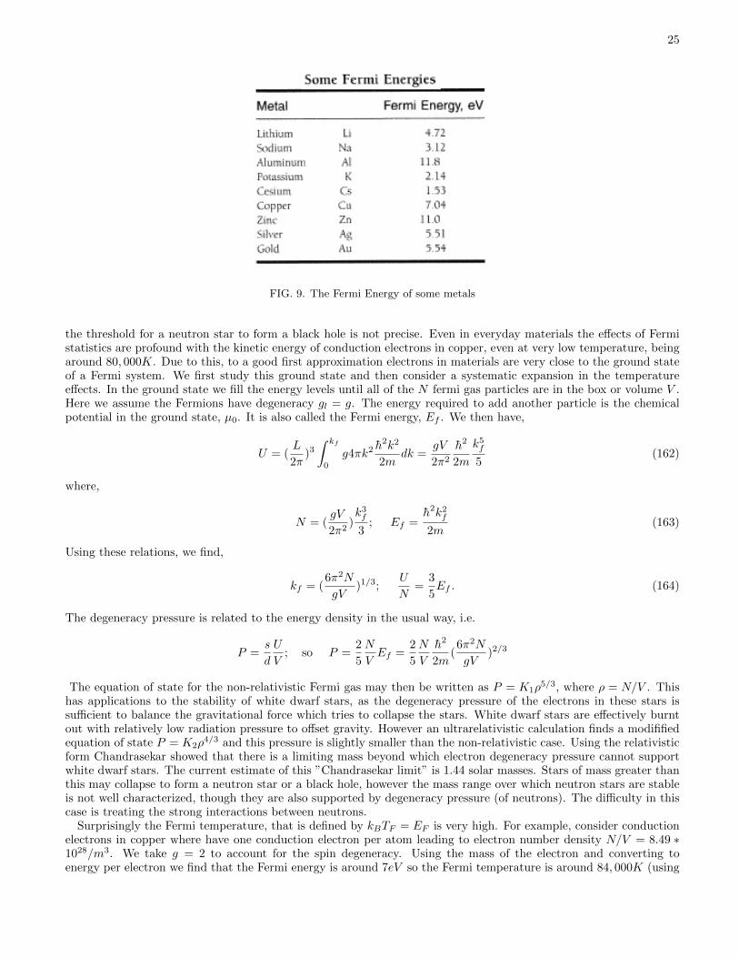
FIG. 9. The Fermi Energy of some metals
the threshold for a neutron star to form a black hole is not precise. Even in everyday materials the effects of Fermistatistics are profound with the kinetic energy of conduction electrons in copper, even at very low temperature, beingaround 80, 000K. Due to this, to a good first approximation electrons in materials are very close to the ground stateof a Fermi system. We first study this ground state and then consider a systematic expansion in the temperatureeffects. In the ground state we fill the energy levels until all of the N fermi gas particles are in the box or volume V .Here we assume the Fermions have degeneracy gl = g. The energy required to add another particle is the chemicalpotential in the ground state, µ0. It is also called the Fermi energy, Ef . We then have,
U = (L
2π)3
∫ kf
0
g4πk2 h2k2
2mdk =
gV
2π2
h2
2m
k5f
5(162)
where,
N = (gV
2π2)k3f
3; Ef =
h2k2f
2m(163)
Using these relations, we find,
kf = (6π2N
gV)1/3;
U
N=
3
5Ef . (164)
The degeneracy pressure is related to the energy density in the usual way, i.e.
P =s
d
U
V; so P =
2
5
N
VEf =
2
5
N
V
h2
2m(6π2N
gV)2/3
The equation of state for the non-relativistic Fermi gas may then be written as P = K1ρ5/3, where ρ = N/V . This
has applications to the stability of white dwarf stars, as the degeneracy pressure of the electrons in these stars issufficient to balance the gravitational force which tries to collapse the stars. White dwarf stars are effectively burntout with relatively low radiation pressure to offset gravity. However an ultrarelativistic calculation finds a modififiedequation of state P = K2ρ
4/3 and this pressure is slightly smaller than the non-relativistic case. Using the relativisticform Chandrasekar showed that there is a limiting mass beyond which electron degeneracy pressure cannot supportwhite dwarf stars. The current estimate of this ”Chandrasekar limit” is 1.44 solar masses. Stars of mass greater thanthis may collapse to form a neutron star or a black hole, however the mass range over which neutron stars are stableis not well characterized, though they are also supported by degeneracy pressure (of neutrons). The difficulty in thiscase is treating the strong interactions between neutrons.
Surprisingly the Fermi temperature, that is defined by kBTF = EF is very high. For example, consider conductionelectrons in copper where have one conduction electron per atom leading to electron number density N/V = 8.49 ∗1028/m3. We take g = 2 to account for the spin degeneracy. Using the mass of the electron and converting toenergy per electron we find that the Fermi energy is around 7eV so the Fermi temperature is around 84, 000K (using

26
300K ≈ 0.025eV ). The Fermi energy and temperature are related to the electron density and this varies considerablyin metals, as seen in the table. Carrying through the calculations to find the degeneracy pressure, we find that forcopper P ≈ 3.8× 10¹⁰N/m2 ≈ 3.5 ∗ 105Atmospheres. The high kinetic energy and pressure of the electrons in metalsare offset by the binding energy of the material. Given that the Fermi temperature is high, we can consider the ratioT/TF to be small in most cases of interest and look for an expansion in this variable.
2. Expansion at ”low” temperatures - Sommerfeld
At low temperatures, βµ is large so the series expansions in Eq. (69) for f3/2 and f5/2 are poorly convergent so weneed a different approach. Following Somerfeld, it is more convenient to carry out an expansion in ν = βµ = ln(z).The procedure is as follows. We work the the integral form of f3/2(z),
f3/2(z) =4
π1/2
∫ ∞0
dx x2 ze−x2
1 + ze−x2 (167)
We change variables to y = x2, then and integrate by parts to find,
f3/2(z) =2
π1/2
∫ ∞0
dyy1/2
ey−ν + 1=
4
3π1/2
∫ ∞0
dyy3/2ey−ν
(ey−ν + 1)2(168)
The integration by parts leads to an integrand that is cnvergent at large y. Now we expand y3/2 in a Taylor seriesabout ν,
y3/2 = (ν + (y − ν))3/2 = ν3/2 +3
2ν1/2(y − ν) +
3
8ν−1/2(y − ν)2 + ... (169)
so that,
f3/2(z) =4
3π1/2
∫ ∞0
dyey−ν
(ey−ν + 1)2(ν3/2 +
3
2ν1/2(y − ν) +
3
8ν−1/2(y − ν)2 + ...). (170)
Defining t = y − ν yields,
f3/2(z) =4
3π1/2
∫ ∞−ν
dtet
(et + 1)2(ν3/2 +
3
2ν1/2t+
3
8ν−1/2t2 + ...) (171)
Now we break the integral up as, ∫ ∞−ν
=
∫ ∞−∞−∫ −ν−∞
(172)
where the second integral is exponentially small, ie. O(e−ν), so we can ignore it. Finally we have,
f3/2(z) =4
3π1/2(ν3/2I0 +
3
2ν1/2I1 +
3
8ν−1/2I2 + ...); where In =
∫ ∞−∞
dttnet
(et + 1)2(173)
I0 = 1, while by symmetry In is zero for odd n. For even n > 0, In is related to the Reimann zeta function, through,
In = 2n(1− 21−n)(n− 1)!ζ(n), with ζ(2) =π2
6, ζ(4) =
π4
90, ζ(6) =
π6
945(174)
At very low temperatures, we take only the leading order term in the expansion so that,
N
V=
1
λ3
4
3π1/2(βµ0)3/2I0 (175)
where µ0 is the leading order expression for the chemical potential at low temperatures. Solving yields,
µ0 = εF =h2
2m
(6π2N
V
)2/3
(176)

27
The fermi energy is calculated directly using,
εF = h2k2F /2m; with N =
(L
2π
)3 ∫ kF
0
4πk2dk (177)
that of course leads to the same result. However the Sommerfeld method enables us to also calculate the temperaturedependence. To find the first temperature dependent term, we take the next term in the expansion of the chemicalpotential.
N
V=
1
λ3
4
3π1/2[(βµ)3/2I0 +
3
8(βµ)−1/2I2 + ...] (178)
We define µ1 to be the next to leading estimate of µ and using I2 = π2/3, find that it is given by,
N
V=
1
λ3
4
3π1/2[(βµ1)3/2 +
3
8
π2
6(βµ0)−1/2]. (179)
which may be written as,
(βµ0)3/2 = (βµ1)3/2 +π2
8(βµ0)−1/2 or (βµ1)3/2 = (βµ0)3/2[1− π2
8(βµ0)−2] (180)
Solving and using βµ0 = βεF gives,
µ1 = εF [1− π2
8
(kBT
εF
)2
]23 = εF [1− π2
12
(kBT
εF
)2
+O(
(kBT
εF
)4
] (181)
It is not too difficult to calculate the next term in the expansion of µ,
µ2 = εF [1− π2
12
(kBT
εF
)2
− π4
80
(kBT
εF
)4
+O(
(kBT
εF
)6
)] (182)
It is then evident that this is a rapidly convergent series for all kT < εF . For many applications this is well satisfied sothe low temperature thermodynamics is deduced from this form of the chemical potential. To find the thermodynamics,we also need an asymptotic expansion for f5/2(z) (see e.g. Pathria and Beale p 236),
f5/2(ν) =8
15π1/2(ν5/2 +
5π2
8ν1/2 + ...) =
8
15π1/2ν5/2(1 +
5π2
8ν−2 + ...) (183)
From Eq. (70) to leading order in the temperature we write,
U =3kBTV
2λ3
8
15π1/2(βµ1)5/2(1 +
5π2
8(βµ0)−2) =
3kBTV
2λ3
8(βµ0)5/2
15π1/2[(1− 5π2
24(βµ0)−2)](1 +
5π2
8(βµ0)−2) (184)
Using a leading order expansion and some work on the prefactor we find,
U =3
5NεF [1 +
5
12π2
(kBT
εF
)2
] (185)
The specific heat is then,
CVNkB
=π2
2
kBT
εF(186)
and the equation of state is,
PV =2
3U =
2
5NεF [1 +
5
12π2
(kbT
εF
)2
] (187)
Note that at the densities typical of metals, and at room temperature, the electrons at the Fermi energy have velocitiescharacteristic of a classical gas with temperatures roughly 10, 000K. This is due to the pecular nature of the exchangeinteraction, or Pauli principle. For this reason high density Fermi systems become more ideal as their density increasesas in that limit, the exchange interaction dominates.
The Fermi factor is the average number of particles in each energy level,
< np >=1
exp(β(ε− µ)) + 1(188)
At low temperatures, this function approaches a step function, where states below the Fermi energy, εp < εF , are fullyoccupied, while those above the Fermi energy are unoccupied. The width of the step function is given by kBT/εF .

28
IV. MODELING OF THE BEHAVIOR OF METALS
In some metals the electrons near the Fermi energy can be treated as a free Fermi gas. For example, this approxi-mation is very good Alkali metals that have one electron in an outer s orbital. The free electron model is also a goodstarting point for more complex metals where band structure effects become important and for strongly correlatedsystems where Coulomb interactions between the electrons plays a key role. In many materials the Debye model pro-vides a useful approximation of the contribution of phonons to the thermodynamic properties. The thermodynamicbehavior of metals can therefore, to first approximation, be considered to be a sum of the contribution due to phononsand a contribution due to electrons. For the specific heat this leads to the prediction that at low temperatures,
CVNkB
=π2
2
kBT
εF+
12π4
5
(T
TD
)3
(189)
which is a sum of the electron contribution and the phonon contribution. This provides a good approximation whenband structure effects, interaction effects and disorder effects are not important, and provided T << TD.
V. GENERALIZED SOMMERFELD EXPANSION
The Sommerfeld expansion is easily generalized to high order in any spatial dimension and for a wide rangeof dispersion relation. We consider the general dispersion relation εk = cεk
s, which for s = 1, cε = hc is theultrarelativistic case, while s = 2, cepsilon = h2/2m is the non-relativistic case. We carry out the Sommerfeldexpansion for N and U in general dimension starting with,
N = g(L
2π)d∫ ∞
0
cdkd−1 ze−βεk
1 + ze−βεk; U = g(
L
2π)d∫ ∞
0
cdkd−1cεk
s ze−βεk
1 + ze−βεk(190)
where g is the degeneracy. Now we use,
x = βεk = βcεks; k = (
x
βcε)1/s; dk =
1
sx(x
βcε)1/s (191)
which leads to,
N = g(L
2π)dCds
(1
cεβ)d/s
∫ ∞0
dxxd/s−1
ex−ν + 1; U = gkBT (
L
2π)dCds
(1
cεβ)d/s
∫ ∞0
dxxd/s
ex−ν + 1; (192)
We then carry out the Sommerfeld expansion for the integral,
J(α) =
∫ ∞0
dxxα−1
ex−ν + 1=
1
α
∫ ∞0
dxxαex−ν
(ex−ν + 1)2(193)
where the last expression is found by integrating by parts. Now we use the expansion,
xα = (ν + (x− ν))α =∞∑l=0
α!
l!(α− l)!να−l(x− ν)l (194)
so that,
J(α) =1
α
∞∑l=0
α!
l!(α− l)!να−lIl (195)
where,
Il =
∫ ∞−ν
dttlet
(et + 1)2=
∫ ∞−∞
dttlet
(et + 1)2+O(e−ν) (196)
The values for Il are given in Eq. (174) above. For the N equation we use α = d/s, while for the energy equation weuse d/s+ 1.

29
Assigned problems and sample quiz problems
Sample Quiz Problems
Quiz Problem 1. Write down the equation for the thermal de Broglie wavelength. Explain its importance in thestudy of classical and quantum gases.
Quiz Problem 2. Why are the factors 1/N ! and 1/h3N introduced into the derivation of the partition function ofthe ideal classical gas?
Quiz Problem 3. Explain why the heat capacity at constant volume of a nitrogen molecule is roughly 1.5NkB at1K but 2.5NkB at room temperature. What are the expressions for the heat capacity at constant pressure for thesetwo cases?
Quiz Problem 4. In modeling the earth’s atmosphere using the equilibrium isothermal model, the gas pressuredecreases exponentially with altitude. Explain how this is reconciled with the equilibrium condition of constantpressure found in our discussion of thermodynamics in Part 1 of the course.
Quiz Problem 5. Discuss the assumptions used in the isothermal and adiabatic models of the atmosphere.
Quiz Problem 6. What is the Curie law? Derive this law for the spin half Ising paramagnet.
Quiz Problem 7. Paramagnets and also the Ising model in one dimension exhibit a peak in their specific heat,with the low temperature behavior being an approach to zero exponentially and at high temperature an approachto zero as 1/T 2. What is there a peak in the specific heat in these models. What can’t we use the rule kBT/2 perdegree of freedom?
Quiz Problem 8. Explain the meaning of negative temperature in the Ising paramagnetic and how it can be usedto make a magnetic cooling device.
Quiz Problem 9. What is the meaning of the terms “spontaneous symmetry breaking” (or spontaneous magne-tization) and “breaking of ergodicity” in the context of the two dimensional Ising model.
Quiz Problem 10. State and give a physically explanation of the behavior of the chemical potential µ and the fu-gacity z = eβµ as temperature T →∞, for both the Bose gases. Compare the cases of photons, phonons and Helium 4.
Quiz Problem 11. Write down the starting expression in the derivation of the grand partition function, ΞB forthe ideal Bose gas, for a general set of energy levels εl. Carry out the sums over the energy level occupancies, nl andhence write down an expression for ln(ΞB), and the average occupancy of each energy level < nl >.
Quiz Problem 12. In the condensed phase superfluids are often discussed in terms of a two fluid model. Basedon the analysis of the ideal Bose gas, explain the physical basis of the two fluid model.
Quiz Problem 13. Why is the chemical potential of photons in a box, and also acoustic phonons in a crystal,taken to be zero?
Quiz Problem 14. Write down the blackbody energy density spectrum.
Quiz Problem 15. Write down and explain the relationship between the intensity of radiation emitted by ablackbody (Stefan-Boltzmann law) and the energy density of a photon gas in the blackbody.
Quiz Problem 16. Explain the physical origin of the cosmic microwave background (CMB) blackbody spectrumof the universe. It is currently at a temperature of TCMB = 2.713K. If the universe is expanding at a constant rateL(t) = H0t, where H0 is a constant what is the expected behavior of the temperature TCMB(t).
Quiz Problem 17. Derive or write down the spectral energy density for blackbody radiation in a universe withtwo spatial dimensions.

30
Quiz Problem 18. Derive or write down the Debye theory for the internal energy for phonons in a square lattice.Derive the low and high temperature limits of the internal energy and specific heat for this system.
Quiz Problem 19. On a graph, illustrate the behavior of the chemical potential µ and the fugacity z = eβµ as afunction of temperature. What is the chemical potential and fugacity of the the Fermi and Bose gases as temperatureT →∞ and as T → 0.
Quiz Problem 20. Write down the starting expression in the derivation of the grand partition function, ΞF forthe ideal Fermi gas, for a general set of energy levels εl. Carry out the sums over the energy level occupancies, nl andhence write down an expression for ln(ΞF ).
Quiz Problem 21. White dwarf stars are stable due to electron degeneracy pressure. Explain the physical originof this pressure.
Assigned problems
Assigned Problem 1. From the density of states for an ideal monatomic gas Ω(E) given in Eq. (26) of the notes,find the Sackur-Tetrode equation for the entropy, Eq. (27) of the notes.
Assigned Problem 2. Using the canonical partition function for the ideal gas, show that,
(δE)2 = kBT2Cv (197)
Assigned Problem 3. Using the grand partition function of the ideal classical gas show that,
(δN)2 = NkBTρκT (198)
Assigned Problem 4Consider a gas of N atoms in volume V . Each atom has one unpaired electron in its outer energy level that is a zero
angular momentum state, i.e. the ground state is l = 0 and has an unpaired electron. A magnetic field is applied tothis gas. Write down the canonical and grand canonical partition functions of this system taking into account center ofmass and spin degrees of freedom, assuming that the magnetic interaction is paramagnetic with no spin-orbit coupling.
Assigned Problem 5.Consider a gas where each atom can have one of two energy levels ε0 and ε1. Find the average energy per particle
taking into account the ideal monatomic gas behavior and the two internal energy levels. Find the specific heat ofthe system in the limits T → 0 and T →∞.
Assigned Problem 6.Consider a dissociating system at thermal equilibrium, where,
A ⇐⇒ B +B (199)
Ignore the internal degrees of freedom of both species and take the mass of an A particle to be twice that of a Bparticle. Given that N = 2NA +NB is fixed, that the volume is fixed, and that the binding energy of A is ε, find thetemperature dependence of NA and NB and find a simple expression for the ratio < NB >2 / < NA >.
Assigned Problem 7.Calculate the specific heat of the model defined by the Hamiltonian Eq. (51) of the text. Is there a peak in the
specific heat? Why or why not?
Assigned Problem 8.Generalize the transfer matrix method for the one dimensional Ising model to the case of an applied field (i.e.
combine the Hamiltonians in Eq. (41) and (55)) and calculate the magnetic susceptibility at low field. Does it obeya Curie law?
Assigned Problem 9.Consider the Peierls argument for the two dimensional spin half Ising model on a square lattice, where the topo-
logical excitation is a flat domain wall dividing a domain of up spins and down spins. Does this argument suggest

31
that finite temperature spontaneous symmetry breaking is possible in the two dimensional Ising model?
Assigned Problem 10.By using the Maxwell-Boltzmann statistics to fill the energy levels of a particle in a box, show that the grand
partition function found in this way is the same as that found by carrying out the classical phase space integrals.
Assigned Problem 11. At high temperatures we found that the ideal Bose gas reduces to the ideal classical gas.Derive the next term in the expansion of the equation of state of the ideal Bose gas at high temperatures, and verifythat,
PV
NkBT= 1− 1
25/2
λ3N
V+ .... (200)
The pressure of the ideal Bose gas is loser than that of the classical gas at the same temperature and volume. Why?
Assigned Problem 12. Using the general forms of the Bose gas equations, discuss the behavior of the Bose gasat low temperatures in one and two dimensions for the case of a non-relativistic gas. Is a finite temperature Bosecondensation predicted ? Show that at high temperatures the equation of state reduces to the ideal classical gas?Explain your reasoning.
Assigned Problem 13. For the 3-D non-relativistic case: a) Find the entropy of the ideal Bose gas in thecondensed phase T < Tc. Is this entropy higher or lower than the classical ideal gas under the same conditions?Explain your result.
Assigned Problem 14. Show that a d − dimensional Bose gas with dispersion relation εp = cps obeys therelation,
P =s
d
U
V(201)
Assigned Problem 15. Find the entropy of a photon gas in d dimensions. Show that the entropy per photon isindependent of temperature - explain your result.
Assigned Problem 16. Find the thermodynamic properties, PV , U , S, CV of the Debye phonon model in ddimensions.
Assigned Problem 17. Carry through the analysis of the Bose gas for the case of massive ultrarelativisticparticles where µ 6= 0. What is the lower critical dimension for a BEC transition in this case?
Assigned Problem 18. At high temperatures we found that the ideal quantum gases reduce to the ideal classicalgases. Derive the next term in the expansion of the equation of state of the ideal Fermi gas at high temperatures,and verify that,
PV
NkBT= 1 +
1
25/2
λ3N
V+ .... (202)
The pressure of the ideal Fermi gas is higher than that of the classical gas at the same temperature and volume.Why? Carry out a similar expansion for the Bose gas. Is the pressure higher or lower than the ideal classical gas atthe same values of T, V ? Why?
Assigned Problem 19. By expanding the denominator of the integral, 1/(1− y) for small y = ze−x2
show that,
f3/2(z) =4
π1/2
∫ ∞0
dx x2 ze−x2
1 + ze−x2 =
∞∑l=1
(−1)l+1zl
l3/2(203)
Assigned Problem 20. Derive expressions for Z, Ξ, PV , µ and U for the classical gas in one and two dimensions.Are the results what you expect? How do they compare with the result in three dimensions. White general expressionsthat are valid in any dimension.

32
Assigned Problem 21. Derive expressions for Ξ, PV , N/V and U for the Fermi gas in one and two dimensions.White general expressions that are valid in any dimension. Find the leading order terms in the high temperatureexpansions for these quantities. Are the results what you expect? How do they compare with the result in threedimensions, and with the classical gas.
Assigned Problem 22. Show that a d − dimensional Fermi gas with dispersion relation εp = cps obeys therelation,
P =s
d
U
V(204)
Quiz Problem 23. Find the first two terms in the low temperature behavior of the internal energy an ultrarela-tivistic Fermi gas at low temperature. From your expression for the internal energy, find the specific heat of the gas.Compare the pressure of the gas to that of a non-relativisitic gas with the same density.