statistical process control, part 2: how and why spc works

Scott Leavengood, Extension agent, KlamathCounty; and James E. Reeb, Extension forestproducts manufacturing specialist; Oregon StateUniversity.

Part 2:How and Why SPC Works S. Leavengood and J. Reeb

PERFORMANCE EXCELLENCEIN THE WOOD PRODUCTS INDUSTRY

EM 8733-E • June 1999$3.00

Part 1 in this series introduced Statistical Process Control (SPC) bydiscussing the history, philosophy, and benefits of SPC, by suggestinghow to successfully implement a new SPC program, and by attemptingto alleviate fears of the math associated with SPC.

The goal for Part 2 is to build management understanding andconfidence in SPC as a profit-making tool. It is unreasonable to expectmanagers to commit to and support SPC training and implementationif they do not understand what SPC is and how and why it works. Thispublication discusses the importance of understanding and quantifyingprocess variation and describes how and why SPC works.

Part 3 in the series is a step-by-step approach to building the skillsrequired to implement SPC. Later publications in the series willpresent case histories of SPC use in wood products firms, examiningpitfalls and successful approaches and providing real-world evidenceof SPC’s benefits as a process improvement tool.

Variation—it’s everywhereVariation is a fact of life. It is everywhere, and it is unavoidable.

Even a brand-new, state-of-the-art machine cannot hold perfectly to thetarget setting; there always is some fluctuation around the target.Attaining consistent product quality requires understanding, monitor-ing, and controlling variation. Attaining optimal product qualityrequires a never-ending commitment to reducing variation.

Where does variation come from? Walter Shewhart, the man whosework laid the foundations for SPC, recognized that variation has twobroad causes: common (also called chance, random, or unknown)causes and special (also called assignable) causes.

Common causes of variation are inherent in the process and can bethought of as the “natural rhythm of the process.” Common causes are

Archival copy. Information is out of date. For current information, see OSU Extension Catalog: https://catalog.extension.oregonstate.edu/em8733

2

STATISTICAL PROCESS CONTROL

evidenced by a stable, repeating pattern of variation. Real qualityimprovement requires a continual focus on reducing common-cause variation.

Special causes of variation are a signal that something haschanged in the process. Special causes are evidenced by a disrup-tion of the stable, repeating pattern of variation. Special causes ofvariation result in unpredictable process performance and musttherefore be identified and removed before taking other steps toimprove quality.

Why is it important to distinguish between these two types ofvariation? Because the remedies are completely different. Under-standing the difference between the two types of variation helpsmanufacturers to target quality improvement efforts correctly andthereby avoid wasted effort and expense.

SPC in a nutshellMontgomery (1997) defines SPC as “...a powerful collection of

problem-solving tools useful in achieving process stability andimproving capability through the reduction of variability.” Controlcharts and process capability analysis are the two primary tools ofSPC. Other tools such as histograms, flow charts, cause-and-effectdiagrams, check sheets, and Pareto diagrams also are useful inquality and process improvement.

In discussing how and why SPC works, we will:• Describe the distribution of the process• Estimate the limits within which the process operates under

“normal” conditions• Determine whether the process is stable• Continue to monitor and control the process• Compare process performance to specifications, and• See how to continuously improve the process

The distribution of the processIn SPC, when we talk about the distribution of the process, we

are referring not to the process itself but to data collected from theprocess—for example, data on widths of pieces coming out of awoodworking machine—and to the way those data are distributedwhen plotted on a chart or graph.

Describing the distribution of a process is analogous to evaluat-ing your marksmanship. How’s your aim? Are you accurate—inother words, are you on target? Is your aim precise; that is, are all

Real qualityimprovement …

requires acontinual focus onreducing common-cause variation.


3

HOW AND WHY SPC WORKS

the shots clustered around the target, or are they distributed all overthe place (Figure 1)? In manufacturing, the questions are:• Where is the process centered; in other words, is the process on

or off target and, if it’s the latter, by how much is it off target?• How much does the process fluctuate about the center?

HistogramsHistograms are visual tools to examine distributions. A histo-

gram is a bar graph that shows how frequently data fall withinspecific cells, that is, ranges of values. Histograms make it rela-tively simple to estimate where the process is centered and howmuch fluctuation there is about the center.

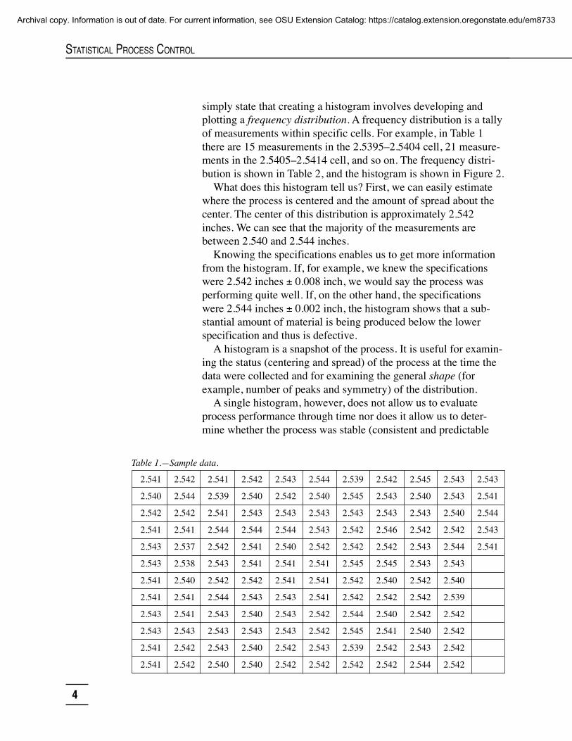
Table 1 (Page 4) shows measurements of widths (in inches) of125 wood components produced by a woodworking machine.

We must have data to know how a process is performing. How-ever, it is difficult to derive much information from data as pre-sented in Table 1. The data would provide more information if theywere grouped, organized, and displayed graphically. A histogramdoes just that.

We will leave the detailed discussion of how to create histo-grams for a future publication. For our purposes here, we will

Figure 1.—Precision and accuracy (adapted from Montgomery, 1997).

Neither precise nor accurate Accurate but not precise

Precise but not accurate Precise and accurate


4


simply state that creating a histogram involves developing andplotting a frequency distribution. A frequency distribution is a tallyof measurements within specific cells. For example, in Table 1there are 15 measurements in the 2.5395–2.5404 cell, 21 measure-ments in the 2.5405–2.5414 cell, and so on. The frequency distri-bution is shown in Table 2, and the histogram is shown in Figure 2.

What does this histogram tell us? First, we can easily estimatewhere the process is centered and the amount of spread about thecenter. The center of this distribution is approximately 2.542inches. We can see that the majority of the measurements arebetween 2.540 and 2.544 inches.

Knowing the specifications enables us to get more informationfrom the histogram. If, for example, we knew the specificationswere 2.542 inches ± 0.008 inch, we would say the process wasperforming quite well. If, on the other hand, the specificationswere 2.544 inches ± 0.002 inch, the histogram shows that a sub-stantial amount of material is being produced below the lowerspecification and thus is defective.

A histogram is a snapshot of the process. It is useful for examin-ing the status (centering and spread) of the process at the time thedata were collected and for examining the general shape (forexample, number of peaks and symmetry) of the distribution.

A single histogram, however, does not allow us to evaluateprocess performance through time nor does it allow us to deter-mine whether the process was stable (consistent and predictable

Table 1.—Sample data.

2.541 2.542 2.541 2.542 2.543 2.544 2.539 2.542 2.545 2.543 2.543

2.540 2.544 2.539 2.540 2.542 2.540 2.545 2.543 2.540 2.543 2.541

2.542 2.542 2.541 2.543 2.543 2.543 2.543 2.543 2.543 2.540 2.544

2.541 2.541 2.544 2.544 2.544 2.543 2.542 2.546 2.542 2.542 2.543

2.543 2.537 2.542 2.541 2.540 2.542 2.542 2.542 2.543 2.544 2.541

2.543 2.538 2.543 2.541 2.541 2.541 2.545 2.545 2.543 2.543

2.541 2.540 2.542 2.542 2.541 2.541 2.542 2.540 2.542 2.540

2.541 2.541 2.544 2.543 2.543 2.541 2.542 2.542 2.542 2.539

2.543 2.541 2.543 2.540 2.543 2.542 2.544 2.540 2.542 2.542

2.543 2.543 2.543 2.543 2.543 2.542 2.545 2.541 2.540 2.542

2.541 2.542 2.543 2.540 2.542 2.543 2.539 2.542 2.543 2.542

2.541 2.542 2.540 2.540 2.542 2.542 2.542 2.542 2.544 2.542


5


Cell Cellboundaries midpoint Frequency

2.5365 – 2.5374 2.537 12.5375 – 2.5384 2.538 12.5385 – 2.5394 2.539 42.5395 – 2.5404 2.540 152.5405 – 2.5414 2.541 212.5415 – 2.5424 2.542 352.5425 – 2.5434 2.543 322.5435 – 2.5444 2.544 102.5455 – 5.5454 2.545 52.5455 – 2.5464 2.546 1

Table 2.—Frequency distribution for data in Table 1.

performance) when the data were collected. Also, it takes time tocollect the data (mathematicians suggest at least 50 to 100 datapoints per histogram) which can become overwhelming if it has tobe done every day.

To be practical for day-to-day process control, we need a sys-tem in which relatively small samples allow us to decide whetherthe process is okay and therefore should be left alone, or whetherproblems are beginning to arise and we should take action. SPCprovides such a system through the use of control charts.

2.537 2.538 2.539 2.540 2.541 2.542 2.543 2.544 2.545 2.546

35

30

25

20

15

10

5

0

Widths (inches)

Freq

uenc

y

Figure 2.—Histogram for data in Table 1.

A histogram. . .

is a useful snapshot ofthe process, but itdoesn’t let us evaluatethe process over timeor determine whetherthe process is stable.


6


Control chartsControl charts are an SPC tool used to monitor and control

processes. There are charts for variables data (measurement datasuch as length, width, thickness, and moisture content) and chartsfor attributes data (“counts” data such as number of defective unitsin a sample or number of errors on an invoice). We’ll focus here onone type of variables control chart and will discuss the other kindsin future publications.

In general, control charts are used as follows: samples are takenfrom the process, statistics (for example, average and range) arecalculated and plotted on charts, and the results are interpretedwith respect to process limits—or, as they are known in SPCterminology, control limits. Control limits are the limits withinwhich the process operates under normal conditions. They tell ushow far we can expect sample values to stray from the averagegiven the inherent variability of the process—or, to use the SPCterms, the magnitude of common-cause variation. Data pointsbeyond the control limits or other unusual patterns indicate special-cause variation.

Estimating control limitsCalculating control limits requires only two numbers: an esti-

mate of central tendency (process centering), and an estimate ofprocess variation.

The average is our best estimate of central tendency. The aver-age is widely used and is understandable to most people. Forexample, golfers and bowlers routinely calculate averages from alist of scores. To find an average, add all the sample measurementsand divide the sum by the sample size. As an example, let’s use thefirst five sample measurements in Table 1:

2.541 + 2.540 + 2.542 + 2.541 + 2.543 = 12.707 = 12.707 ÷ 5

= 2.541 (rounded to three decimal places)

where (pronounced “X-bar”) is the symbol used for the average.

In addition to a measure of central tendency, we need a measureof variation. The values commonly used to quantify variation arethe standard deviation and the range.

SPC uses the range more often than the standard deviationbecause calculating the standard deviation is fairly involved. Also,the standard deviation usually is a less familiar concept for most

×

××

Control limits…tell us how far we canexpect sample valuesto stray from theaverage, given theinherent variability ofthe process.


7


people. The range (R), on the other hand, is simply the largestvalue (Xmax) in the sample minus the smallest value (Xmin) in thesample. For the five-sample measurements listed above, Xmax =2.543 and Xmin = 2.540, and therefore:

R = 2.543 – 2.540 = 0.003We now have the two values we need to calculate the control

limits—a measure of central tendency (the average, ) and ameasure of variation (the range, R). Recall that control limits tellus how far we can expect sample values to stray from the average,given the magnitude of process variation. Therefore, the formula forthe control limits must account for both the average and the range. Afrequency distribution allows us to develop such a formula.

Frequency distributions and probabilityRecall that Table 2 was the frequency distribution for the data in

Table 1. The science of statistics provides us with a number offrequency distributions with known probabilities. In commonlanguage, probabilities quantify the odds or likelihood of a specificevent. For example, the probability of getting the ace of spades in asingle draw from a deck of cards is 1/52 (1 of 52 possible out-comes), or approximately 0.019. The probability of winning thelottery is often on the order of 1 in 1,000,000 (0.000001). As youcan see, the smaller the probability, the less likely the event.

Statistics science also enables us to determine the probabilitythat something will not happen. For example, the probability of notgetting the ace of spades in a single draw from a deck of cards is1 minus the fraction that indicates the probability of getting the aceof spades, which is 1 minus 1⁄52 (or 0.019), which is 0.981. Formore information on probability, see OSU Extension publicationEM 8718, An Introduction to Models and Probability Concepts.

In SPC, we use known frequency distributions to establish con-trol limits with known probabilities. Control limits are establishedso that the probability of obtaining a value (that is, a result) beyondthe limits is very small unless the process changes significantly.Therefore, control limits minimize false alarms—that is, searchingfor problems when none exists. Searching for problems is oftenexpensive because it involves time, effort, and, in many cases,equipment downtime. Minimizing false alarms and their expense isa key benefit of SPC and is the prime reason the first book on SPCwas titled “Economic Control of Quality of Manufactured Product”(Shewhart, 1931).

×


8


The normal distributionThe normal* distribution is a frequency distribution used exten-

sively in SPC. The normal distribution commonly is called the bellcurve due to the curve’s shape (Figure 3). Only two parameters areneeded to construct a normal distribution: the average and thestandard deviation. The average is designated with the Greeklowercase letter µ (mu), and the standard deviation is designatedwith the Greek lowercase letter σ (sigma). The normal curve’speak is at the average, µ, and its spread (the width of the curve) isreflected by the standard deviation, σ. The parameters µ and σgenerally are unknown, and thus we have to estimate them bysampling the process. We use , the sample average, to estimate µ,and we use R, the sample range, to estimate σ.

In SPC, the normal distribution allows us to determine theprobabilities of getting values beyond control limits. Probabilityvalues for the normal distribution can be found in textbooks onstatistics and quality control. For purposes of our brief discussionof normal distribution, we simply will state some common proba-bilities.

The probability that a normally distributed variable will bewithin plus or minus 1 standard deviation (1σ, pronounced “one

×

*Note: “Normal” is the name for the distribution and is not to beconfused with common usage of the word “normal” as meaning“standard” or “commonplace.”

Figure 3.—The normal distribution.

µ – 3σ µ – 2σ µ – 1σ µ + 3σµ + 2σµ + 1σµ

Freq

uenc

y


9


sigma”) of the average is approximately 0.68. That is, 68 percentof the values will be within 1 standard deviation of the average.The probability that a normally distributed variable will be within±2σ of the average is approximately 0.95, and within ±3σ of theaverage is approximately 0.997 (Figure 4).

Figure 4.—The normal distribution, showing common probabilities.

Knowing that 99.7 percent of the values will fall within ±3σ ofthe average, we can feel confident that a value beyond 3σ wouldbe highly unlikely unless a significant change (i.e., special-causevariation) had occurred in the process.

For example, if process output is normally distributed, and theaverage for our process is 2.542, and the standard deviation (σ) is0.002, then the probability of a value between 2.536 and 2.548[that is, 2.542 ± (3 x 0.002)] inches is 0.997. Conversely, theprobability of observing a value less than 2.536 or greater than2.548 is 0.003 (1 – 0.997), or approximately 3 chances in 1,000.Therefore, 2.536 and 2.548 would appear to make good controllimits because a value beyond the limits is statistically rare. There-fore, it is very likely that special causes of variation are influencingthe process, and so searching for problems is likely to be profitable.

So, can we use 2.536 as the lower control limit and 2.548 for theupper control limit? We could—if we were examining individualitems from the process. Recall, however, that we are sampling the

68.0%95.0%

99.7%

µ – 3σ µ – 2σ µ – 1σ µ + 3σµ + 2σµ + 1σµ

Freq

uenc

y


10


process and collecting statistics (in this example, the average) formultiple items* rather than for individual items. Our control charttherefore should reflect the distribution of averages, not of indi-vidual data points.

Individuals vs. averagesThe variation of averages is significantly less than the variation

of the individual values. Figure 5 demonstrates this point by over-laying a histogram of averages of five measurements from the datain Table 1 onto the histogram of individual values.

The larger the sample, the narrower the distribution of sampleaverages. Therefore, control limits for averages will be narrower(closer to the average) than control limits for individual measure-ments. The values needed to calculate control limits have beentabulated and are available in textbooks. To calculate control limits,you need only look up in a table the value that corresponds tosample size, and then perform simple multiplication and addition.

*There are several reasons we prefer to sample multiple itemsversus individual items from the process. One reason is that theCentral Limit Theorem allows us to use the normal distributionregardless of the actual distribution of the process. We will discussthis and the other reasons in detail in future publications.

Figure 5.—Histogram for individual values and for averages of 5 measurements.

2.537 2.538 2.539 2.540 2.541 2.542 2.543 2.544 2.545 2.546

Freq

uenc

y

Width (inches)

40

30

20

10

0

Individual values Averages of 5


11


Control limits vs. specification limitsBefore leaving the issue of control limits, we must address the

often-asked question, “Why can’t we simply use the specificationsfor control limits? Why all this bother with control limits based onstatistical probabilities, 3σ, etc. when all we really want to know ishow much ‘good’ (that is, ‘within the specifications’) productwe’re producing?” There are two primary reasons never to usespecification limits as control limits.

Control limits are established to minimize false alarms. Unlesssome significant change has occurred in the process, a sample valuebeyond a 3σ control limit is a statistical rarity and thus a signal thatspecial-cause variation is influencing the process. Searching forproblems is likely to be profitable. Therefore, control limits must beestablished as a function of the capabilities of the process. In prac-tice, specification limits usually are established by engineers and arenot a function of the capabilities of the process. Control limitsrepresent “what the process can do,” and specification limits repre-sent “what we want the process to do.” To be useful for qualitycontrol, limits must be based on what the process can do.

Another reason never to use specification limits as control limitsis that the former are for individual items, not for averages. Asnoted earlier, the variation for averages is less than the variationfor individual values. Therefore, comparing a sample average to aspecification limit is the proverbial apples-to-oranges comparison.

False alarms (chasing problems that aren’t there) and failing todetect problems are common when specifications instead of controllimits are used on control charts.

Determine whether the process is stableHow can we be sure that the data we use to establish control

limits are not simply a snapshot of an unstable process? If theprocess is not stable, we are shooting at a moving target, and ourcontrol limits are meaningless for long-term process control.Therefore, we must find a way to determine whether the process isstable. In SPC terminology, we ask, “Is the process in statisticalcontrol?” Or, more simply, “Is it in control?”

In common usage, the phrase “in control” generally describes adesirable situation, and it has the same connotation in SPC. On theother hand, the phrase “out of control” brings forth images ofmayhem—machines on fire, nuts and bolts flying through the air,etc. An out-of-control process, as the phrase is used in SPC, is notquite so dramatic.

Control limits …represent “what theprocess can do.”Specification limitsrepresent “what wewant the process todo.”


12


Deming (1982) defines control in SPC:A stable process, one with no indication of a special causeof variation, is said to be, following Shewhart, in statisticalcontrol, or stable. It is a random process. Its behavior in thenear future is predictable.

Therefore, out of control can be defined as a process that isunder the influence of special causes of variation. Its behavior isnot predictable. Statistically rare occurrences are signals that aprocess is out of control. When a process is out of control, weshould investigate to find and eliminate the special causes ofvariation in order to bring the process back in control and therebyimprove consistency of product quality.

In our discussion of the normal distribution, above, we statedthat upper and lower control limits in SPC generally were set atplus or minus 3 standard deviations (± 3σ) from the average.Finding a normally distributed value beyond the 3σ limits has aprobability of approximately 0.003, which means it is statisticallyrare. Therefore, we can state that a process is out of control if asample value falls outside the control limits.

There are other rules in SPC for determining whether a processis in or out of control. Some companies simply use the “outside thecontrol limits” rule just mentioned; others use several rules thatinvolve detecting trends or “runs” of data points above and belowaverage. For example, eight consecutive data points on the chart onthe same side of the center line (the average) or six consecutivepoints on the chart steadily increasing or decreasing may indicate achange in the process and therefore an out-of-control situation.These additional rules often help to detect problems sooner thanwaiting for a point to fall outside the control limits. For this discus-sion, we will focus simply on the outside-the-control-limits rule.Other rules will be discussed in a future publication.

Now, we have most of the information we need to determinewhether the process is in control. However, for practical applica-tion, one thing is lacking: a visual tool to help us evaluate sampledata and compare them to the control limits. For this purpose,Shewhart created the control chart, also known as the ShewhartControl Chart in honor of its inventor.

Control charts provide a graphical view of the process over time.We will use the data in Table 1 to construct a control chart for theaverage, known as an chart. For purposes of the example, wegroup the measurements in Table 1 into 25 samples with 5 mea-surements per sample. The grouped data are shown in Table 3.

×


13


Table 3. Data from Table 1 organized in samples of 5.

Items in sample* Summary of sample

1 2 3 4 5 R

1 2.541 2.540 2.542 2.541 2.543 2.541 0.003

2 2.543 2.541 2.541 2.543 2.543 2.542 0.002

3 2.541 2.541 2.542 2.544 2.542 2.542 0.003

4 2.541 2.537 2.538 2.540 2.541 2.539 0.004

5 2.541 2.543 2.542 2.542 2.541 2.542 0.002

6 2.539 2.541 2.544 2.542 2.543 2.542 0.005

7 2.542 2.544 2.543 2.543 2.543 2.543 0.002

8 2.540 2.542 2.540 2.543 2.544 2.542 0.004

9 2.541 2.541 2.542 2.543 2.540 2.541 0.003

10 2.543 2.540 2.540 2.543 2.542 2.542 0.003

11 2.543 2.544 2.540 2.541 2.541 2.542 0.004

12 2.543 2.543 2.543 2.542 2.542 2.543 0.001

13 2.544 2.540 2.543 2.543 2.542 2.542 0.004

14 2.541 2.541 2.541 2.542 2.542 2.541 0.001

15 2.543 2.542 2.539 2.545 2.543 2.542 0.006

16 2.542 2.542 2.545 2.542 2.542 2.543 0.003

17 2.544 2.545 2.539 2.542 2.542 2.542 0.006

18 2.543 2.543 2.546 2.542 2.545 2.544 0.004

19 2.540 2.542 2.540 2.541 2.542 2.541 0.002

20 2.542 2.545 2.540 2.543 2.542 2.542 0.005

21 2.543 2.543 2.542 2.542 2.542 2.542 0.001

22 2.540 2.543 2.544 2.543 2.543 2.543 0.004

23 2.540 2.542 2.544 2.543 2.540 2.542 0.004

24 2.539 2.542 2.542 2.542 2.542 2.541 0.003

25 2.543 2.541 2.544 2.543 2.541 2.542 0.003

Averages for all samples

R2.542 0.003

*In practice, measurements should be grouped in a mannerShewhart called “rational subgrouping.” Sampling should be doneso that differences between subgroups (samples) are maximizedand differences within subgroups are minimized. We will discussthis subject in depth in a future publication.

Sample no. ×

×


14


To construct the control chart, we first calculate the average andrange for each sample. We then calculate (pronounced “×-bar-bar” or “× double bar”), which is the average of the 25 sampleaverages, and we calculate , which is the average of the 25sample ranges.

The grand average, , for the 25 sample averages is 2.542inches. We draw a horizontal line across the center of the graph at2.542 to represent the average. is 0.003 inch. As discussedpreviously, to calculate the upper and lower control limits (UCLand LCL, respectively) we use formulas and table values fromtextbooks. Using Table D in Appendix VI in Montgomery (1997),the table value (A2) for a sample size of 5 is 0.577. The controllimits are then:

UCL = + A2

= 2.542 + (0.577 x 0.003)= 2.544

LCL = – A2

= 2.542 – (0.577 x 0.003)= 2.540

We now draw horizontal lines on the graph at the appropriatelocations for the UCL and LCL. Last, data points for each sampleaverage are plotted on the chart (Figure 6).

×

R

×

R

× R

× R

Given that we are attempting to determine whether the process isin or out of control, what can we learn from this chart? Recall thata point outside the control limits or some other unusual patternsindicate the process is out of control. Therefore, Sample 4 indicatesthe process is out of control, and Sample 18 is questionable

1 2 3 4 5 6 7 8 9 10 11 12 13 14 15 16 17 18 19 20 21 22 23 24 25

2.5452.5442.5432.5422.5412.5402.539

Ave

rage

○ ○ ○ ○ ○ ○ ○ ○ ○ ○ ○ ○ ○ ○ ○ ○ ○ ○ ○ ○ ○ ○ ○ ○ ○ ○ ○ ○ ○ ○ ○ ○ ○ ○ ○ ○ ○ ○ ○ ○ ○ ○ ○ ○ ○ ○ ○ ○ ○ ○ ○ ○ ○ ○

Data Average○ ○ ○ ○

UCL LCL

Figure 6.— control chart for data in Table 3.×


15


because it is on the upper control limit.* Had these data beencollected as the process was operating, we would have looked for asource of trouble immediately after we plotted the average ofSample 4. Because the data are historical, we are using the dataonly to determine whether the process is in control.

The chart indicates the process was out of control when the datawere collected. Actions should be taken to identify the problemsthat led to the low value in Sample 4 and the high value in Sample18. After these problems have been identified and corrected, weremove out-of-control samples from the data and recalculate , ,and the control limits. We then redraw the charts and check to seewhether the process is in control now that the out-of-control datapoints have been removed. We continue this process until all datapoints are in control, and then use the resulting limits as trial limitsfor future production.

Had the initial control chart shown that the process was incontrol, the initial control limits would serve as trial control limitsfor future production.

Continue to monitor and control the processFor day-to-day process monitoring, we will collect samples and

plot the results on a control chart using the trial center line andcontrol limits developed above. A data point beyond the limits andunusual patterns will continue to be used as indicators that someaspect of the process has changed and, therefore, as signals that wemust search for special causes of variation. If special causes arefound, corrective actions must be taken.

Due to the hectic pace of the manufacturing environment, it iscommon for long periods to elapse between sample collection and

*In practice, the control chart for variation, the R chart, alwaysshould be constructed and interpreted first to determine whetherthe process is in or out of control. However, we have chosen tosacrifice some technical accuracy in order to reduce the complexityof discussion about multiple control charts. We chose to discuss the chart here rather than the R chart because charts usually areeasier for newcomers to SPC to understand. An chart monitorsthe fluctuation in the process over time—a pretty straightforwardconcept. An R chart, on the other hand, monitors the fluctuation inprocess variability over time; in other words, it monitors thevariability of the variability.

×

× ××

R


16


plotting points on control charts. If an out-of-control situation isindicated, it is likely that defective product has been produced inthe time between problem occurrence and problem detection; thelonger this period, the more defective product has been produced.For control charts to be effective, data should be analyzed, plotted,and interpreted and actions taken as soon as possible. Therefore,control charts should be constructed and interpreted in real time bythe workers on the mill floor, not in the office by managers.

Finally, because control limits are a function of process varia-tion, they should be evaluated periodically and revised whencontrol charts provide evidence that process variation has beenreduced.

Compare process performance to specifications:Process capability analysis

Up to this point, we have concentrated on monitoring what theprocess is doing but have shown little consideration for what wewant the process to do. In other words, we have paid little atten-tion to how the process conforms to specifications.

The fact is, an in-control process can produce defective productif the process is off-target or if the common-cause variation is toohigh. As stated above, the first steps in an SPC program should beto establish control. An out-of-control process is unstable, andtherefore estimates of process performance (centering and varia-tion) are of little use. Only after establishing control can we exam-ine the process’s ability to meet specifications.

Let’s begin with a graphical look at process variation.Figure 7 shows normal curves for two process distributions.

LSL and USL are the lower specification limit and upper specifica-tion limit, respectively. Both processes are centered on the targetdimension. The lower, wider distribution represents a process withrelatively high variation (high standard deviation); the taller,narrower distribution represents a process with lower variation(low standard deviation). The shaded area represents materialoutside specifications.

The advantages of reducing variation are obvious. The processwith lower standard deviation produces far less defective material.From a practical standpoint, however, we need to quantify therelationship between the spread of the process and the spread ofthe specifications. A process-capability analysis does this by usingcapability indices.


17


Figure 7.—Effect of process standard deviation on percentage of product thatdoes not meet specifications.

LSL µ USL (Target)

Defectiveproduct

Defectiveproduct

The first capability index we will discuss is Cp which iscalculated as:

Cp = (USL – LSL) ÷ 6where σ is the process standard deviation and the “^” (pronounced“hat”) symbol over it means “estimate.”

Recall that σ is the true standard deviation for a normallydistributed variable, and generally the best we can do is to estimateit by sampling the process. The value 6 (plus and minus 3σ) isthe total width of process variation. Therefore, Cp is a ratio of thespecification width to total process width.

Continuing the example using the data in Table 1, let’s say ourspecifications are 2.543 inches ± 0.003 inch. Therefore, our LSL is2.540 and our USL is 2.546 inches. To estimate standard deviation( ) we divide (the average range) by d2, a table value found inSPC textbooks. Appendix VI in Montgomery (1997) lists d2 as2.326 for samples of size 5 (i.e., samples of five measurements).Recall our estimate of is 0.003; therefore, is 0.003 ÷ 2.326, or0.001 inch. Cp is then:

Cp = (2.546 – 2.540) ÷ (6 x 0.001) = 1.0

What does this mean? In simple terms, Cp less than 1.0 is “bad”and greater than 1.0 is “good.” That is because a Cp less than 1.0

σ>

σ>

Rσ>

R σ

>


18


indicates that process variation is higher than the specificationwidth, and therefore too much material is defective. A Cp greaterthan 1.0 indicates that process variation is less than the specifi-cation width, and therefore the process can meet the specificationswhile producing minimal defects. Because our Cp is 1.0, we knowthat the process variation is equal to the specification width, andtherefore the process is (just barely) capable of meeting thespecifications.

Cp does not account for process centering relative to the target.(Theoretically, a manufacturing process could be centered far awayfrom the target specification and therefore producing 100% defec-tive product; yet if the process variability were low, Cp wouldindicate everything was okay.)

To account for process variation and for centering relative tothe target, we use another process capability index, Cpk. Theformula for Cpk is:

Cpl = ( – LSL) ÷ 3 , Cpu = (USL – ) ÷ 3

Cpk = min{Cpl, Cpu}

where Cpl and Cpu are the lower and upper process capabilityindices, respectively, relative to the process center; is ourestimate of process centering; and “min” indicates that Cpk is theminimum (lesser) of Cpl and Cpu.

To calculate Cpk, we use as calculated above, and we useas . (Recall that, previously, was calculated as 2.542.) Cpk isthen:

Cpl = (2.542 – 2.540) ÷ (3 x 0.001) = 0.667,

Cpu = (2.546 – 2.542) ÷ (3 x 0.001) = 1.333

Cpk = min{0.667, 1.333} = 0.667

Cpk is interpreted much the same as Cp; that is, below 1.0 is“bad” and above 1.0 is “good.” We get a bit more information withCpk, however. Because Cpl and Cpu are not equal, we know ourprocess is off-center. More specifically, because Cpl is lower thanCpu, we know we are centered too close to the lower specificationlimit. Therefore, excessive defects are produced below the lowerspecification limit. Furthermore, using the normal distribution asan approximation, we can calculate that about 2.3 percent (about2.3 defects per 100) of the material will be defective (out of spec).Calculations of this type will be discussed in a later publication.

>

µ σ>

σ>>

µ

>

µ

σ> ×

>

µ ×

Cp doesn’taccount for…

process centering.In theory, a processcould turn out100% defectiveproduct, yet ifprocess variabilitywere low, Cp wouldbe okay.


19


What if we adjusted the process to put it on target; that is, weshifted the process center ( ) from 2.542 to 2.543 inches? Cp doesnot account for process centering, and so it would not be affected.Cpk, however, would increase from 0.667 to 1.0, meaning that ourdefect rate would decrease from about 2.3 percent to approxi-mately 0.27 percent (about 2.7 defects per 1,000), a very signifi-cant reduction.

In addition to adjusting the process to put it on target, what if wecould reduce process variation from 0.001 to 0.0008 inch? Thiswould result in Cp and Cpk of 1.25. The defect rate would drop to0.009 percent (approximately 9 defects per 100,000). This isobviously a very significant improvement in quality. After obtain-ing cost estimates for scrap and rework, we can calculate the effectthat percentage reductions in defects will have on profit increasesand thus determine the benefits of quality improvement to thebottom line.

The profit increases due to decreases in variation are substantial.The question becomes, how do we reduce variation? The answer:through continuous process improvement.

Continuous process improvementAs stated previously, real quality improvement requires a con-

tinual focus on reducing common-cause variation. Reducingcommon-cause variation is possible only after the process has beenbrought into control.

Process improvement (which leads to quality improvement)requires a more systematic and structured approach than usuallyrequired to remove special causes of variation. Companywidequality improvement requires:• Determining customer needs• Setting quality goals• Developing an improvement strategy• Providing the necessary training and resources• Establishing the organizational infrastructure (quality councils,

teams, etc.)• Reviewing progress, and• Revising the reward system

For these reasons, quality improvement requires the commit-ment and involvement of upper management. Years of experiencehave shown that “delegating quality” is ineffective. Juran (1989)

×


20


provides a thorough treatment of management’s role in qualityplanning, control, and improvement.

ConclusionsThe bottom line is: SPC helps manufacturers increase their

competitiveness and profitability. We have demonstrated SPC’sfoundation in mathematics and statistics to build your understand-ing and confidence in SPC as a profit-making tool and to overcomeany preconceptions that SPC is yet another management fad.

We hope this publication has convinced you that implementingSPC will make your company money, and we hope you willcommit to training your personnel to use SPC. To begin the train-ing process, we refer you to Part 3 in this series, Starting an SPCProgram.


21


For more informationBrown, G.M. and C. Horn. 1982. Quality control programs in

action: A southern pine mill. In: T.D. Brown, ed. Quality Controlin Lumber Manufacturing (San Francisco: Miller Freeman).

Brown, T.D. 1979. Determining lumber target sizes and monitoringsawing accuracy. Forest Products Journal 29(4):48–54.

Brown, T.D. 1982. Determining rough green target size. In: T.D.Brown, ed. Quality Control in Lumber Manufacturing (SanFrancisco: Miller Freeman).

Brown, T.D. 1982. Setting up a size control program. In: T.D.Brown, ed. Quality Control in Lumber Manufacturing (SanFrancisco: Miller Freeman).

Brown, T.D. 1982. Evaluating size control data. In: T.D. Brown,ed. Quality Control in Lumber Manufacturing (San Francisco:Miller Freeman).

Brown, T.D. 1986. Lumber size control. Special Publication No.14, Forest Research Laboratory, Oregon State University,Corvallis, OR. 16 pp.

Cassens, D.L., J.L. Bankston, and J.S. Friday. 1994. Statisticalprocess control of hardwood lumber target sizes: Is it time?Forest Products Journal 44(1):48–50.

Cook, D.F. 1992. Statistical process control for continuous forestproducts manufacturing operations. Forest Products Journal42(7/8):47–53.

Deming, W.E. 1982. Out of the Crisis (Cambridge, MA: Massa-chusetts Institute of Technology Center for Advanced Engineer-ing Study). 507 pp.

Deming, W.E. 1993. The New Economics: For Industry,Government, Education (Cambridge, MA: MassachusettsInstitute of Technology Center for Advanced EngineeringStudy). 240 pp.

Dramm, J.R. 1997. Statistical process control and other tools forcontinuous improvement. In: Proceedings, Wood TechnologyClinic and Show (San Francisco: Miller Freeman).

Dramm, J.R. 1998. Results-driven approach to improving qualityand productivity. In: Proceedings, Wood Technology Clinic andShow (San Francisco: Miller Freeman).


22


Duncan, A.J. 1986. Quality Control and Industrial Statistics, 5th ed.(Homewood, IL: Irwin). 1,123 pp.

Eagan, F.M. 1982. Statistics-based size control in the mill. In: T.D.Brown, ed. Quality Control in Lumber Manufacturing (SanFrancisco: Miller Freeman).

Grant, E.L. and R.S. Leavenworth. 1988. Statistical QualityControl, 6th ed. (New York: McGraw-Hill). 714 pp.

Juran, J.M. 1989. Juran on Leadership for Quality: An ExecutiveHandbook (New York: Macmillan, The Free Press). 376 pp.

Leicester, R.H. 1995. Statistical control for stress graded lumber.In: Proceedings No. 7307, Statistical Process ControlTechnologies: State of the Art for the Forest Products Industry(Madison, WI: Forest Products Society).

Leonard, O.F. 1982. Quality control programs in action: Themedium-sized sawmill. In: T.D. Brown, ed. Quality Control inLumber Manufacturing (San Francisco: Miller Freeman).

Minneci, J. 1995. Control chart implementation in glued laminatedtimber end joint production. In: Proceedings No. 7307,Statistical Process Control Technologies: State of the Art forthe Forest Products Industry (Madison, WI: Forest ProductsSociety).

Moller, D. 1990. Statistical process control (SPC) for dry kilnoperations. In: Proceedings, Western Dry Kiln AssociationJoint Meeting, Reno, NV, May 9–11.

Montgomery, D.C. 1997. Introduction to Statistical QualityControl, 3rd ed. (New York: John Wiley & Sons). 677 pp.

Patterson, D.W. and R.B. Anderson. 1996. Use of statisticalprocess control in the furniture and cabinet industries. ForestProducts Journal 46(1):36–38.

Peck, J. and R. Myers. 1995. SPC in action: Reduction in variationkeys customer satisfaction. In: Proceedings No. 7307,Statistical Process Control Technologies: State of the Art forthe Forest Products Industry (Madison, WI: Forest ProductsSociety).

Schaffer, R.H. and H.A. Thomson. 1992. Successful changeprograms begin with results. Harvard Business Review. Jan.–Feb., pp. 80–89.

Shewhart, W.A. 1931. Economic Control of Quality of Manu-factured Product (Milwaukee, WI: Quality Press). 501 pp.


23


Valg, L. 1965. Analysis of sawing accuracy by statistical qualitycontrol. Research Note No. 51, Faculty of Forestry, Universityof British Columbia, Vancouver. 4 pp.

Walton, M. 1986. The Deming Management Method (New York:Putnam). 262 pp.

Warren, W.G. 1973. How to calculate target thickness for greenlumber. Information Report VP-X-112, Department of theEnvironment, Canadian Forestry Service, Western ForestProducts Laboratory, Vancouver, BC. 11 pp.

Western Electric Co. 1956. Statistical Quality Control Handbook.(Milwaukee, WI: Quality Press). 328 pp.

Whitehead, J.C. 1978. Procedures for developing a lumber sizecontrol system. Information Report VP-X-184, Department ofthe Environment, Canadian Forestry Service, Western ForestProducts Laboratory, Vancouver, BC. 15 pp.

Young, T.M. and P.M. Winistorfer. 1999. Statistical process controland the forest products industry. Forest Products Journal49(3):10–17.

Yuhas, J. 1982. Quality control programs in action: A large sawmillcomplex. In: T.D. Brown, ed. Quality Control in LumberManufacturing (San Francisco: Miller Freeman).


24


GlossaryAssignable causes of variation—See special causes of variation.

Attributes data—Qualitative data that can be counted for recordingand analysis. Results may be recorded as yes/no, go/no go, ordefective/not defective. Examples include percent defective in asample and number of blemishes on a surface.

Arithmetic mean—See average.

Average—A measure of location or central tendency which is thesum of the observed values divided by the number of observa-tions. Also called the arithmetic mean or, simply, the mean.

Bell curve—Common name for the normal distribution, a namederived from the shape of the curve.

Cell—A grouping of values between specified upper and lowerboundaries used to create frequency distributions.

Center (centered, centering)—A numerical value that is “typical”for a set of data. Values used include the average, the median,and the mode.

Central tendency—See center.

Chance causes of variation—See common causes of variation.

Common causes of variation—Sources of variation that affect allthe individual values of the process output being studied. Thesources generally are numerous and individually of small impor-tance but cannot be detected or identified. Also called chance,random, and unknown causes of variation.

Control (statistical)—The condition that exists after a process inwhich all special causes of variation have been eliminated andonly common causes remain.

Control chart—A graphic representation of a characteristic of aprocess, showing plotted values of some statistic gathered fromthe characteristic, a central line, and one or two control limits.Used to determine whether a process is in statistical control andto help maintain statistical control.

Control limits—On a control chart, the criteria for signaling theneed for action, or for judging whether a set of data does or doesnot indicate a “state of statistical control.” Control limits arecalculated from process data and are not to be confused withspecification limits.


25


Distribution—See frequency distribution.

Frequency distribution—A tally of the count, or frequency, ofoccurrences of data in specific cells.

Histogram—A bar chart for displaying a frequency distribution.

In control—See control (statistical).

Mean—See average.

Median—The value at the midpoint in the ordered range of values:half the values are greater than the median value, and half thevalues are less than the median value.

Mode—The most frequently observed value.

Normal distribution—A continuous, symmetrical, bell-shapedfrequency distribution for variables data that underlies controlcharts for variables.

Out of control—The absence of conditions described in control(statistical).

Probability—A scientific discipline whose objective is to studyuncertainty. Probability is the likelihood (commonly called the“odds”) that a specific event will occur.

Process limits—See control limits.

Random causes of variation—See common causes of variation.

Range—A measure of dispersion; the difference between thelargest observed value and the smallest observed value in agiven sample.

Sample—A group of items, observations, test results, or portions ofmaterial taken randomly from a larger collection of items,observations, test results or quantities of material, which provideinformation that may be used as a basis for making a decisionabout the larger collection. See also subgroup.

Special causes of variation—Sources of variation that are intermit-tent, unpredictable, and unstable and that can be detected andidentified.

Specification limits—The engineering requirement for judgingacceptability of a particular characteristic. Specifications are notto be confused with control limits.

Spread—General term describing the dispersion or variability in adata set. Commonly measured with the range or standarddeviation.


26


Standard deviation (sample)—A measure of dispersion, calculatedas the square root of the sum of the squared deviations of obser-vations from their average divided by one less than the numberof observations. The range often is used to estimate the standarddeviation.

Subgroup—In process control applications, generally synonymouswith sample.

Unknown causes of variation—See common causes of variation.

Variables data—Quantitative data, where measurements are usedfor analysis. Examples include length, width, thickness, viscos-ity, strength (e.g., pounds per square inch, or psi), and density.


27


This publication is part of a series, PerformanceExcellence in the Wood Products Industry. The variouspublications address topics under the headings of woodtechnology, marketing and business management,production management, quality and process control,and operations research.

To view and download any of the other titles in theseries, visit the OSU Extension Web site at http://eesc.oregonstate.edu/ then “Publications & Videos” then“Forestry” then “Wood Processing” and “BusinessManagement”. Or, visit the OSU Wood Products ExtensionWeb site at http://wood.oregonstate.edu/

PERFORMANCE EXCELLENCEIN THE WOOD PRODUCTS INDUSTRY

ABOUT THIS SERIES


http://extension.oregonstate.edu/catalog/index.php

28


© 1999 Oregon State University

This publication was produced and distributed in furtherance of the Acts of Congress of May 8 and June 30, 1914. Extensionwork is a cooperative program of Oregon State University, the U.S. Department of Agriculture, and Oregon counties. OregonState University Extension Service offers educational programs, activities, and materials—without regard to race, color, religion,sex, sexual orientation, national origin, age, marital status, disability, and disabled veteran or Vietnam-era veteran status—asrequired by Title VI of the Civil Rights Act of 1964, Title IX of the Education Amendments of 1972, and Section 504 of theRehabilitation Act of 1973. Oregon State University Extension Service is an Equal Opportunity Employer.

Published June 1999.


statistical process control, part 2: how and why spc works

Documents