Statistical Process Control UsingTwo Measurement Systems

Stefan H. SteinerDept. of Statistics and Actuarial Sciences

University of WaterlooWaterloo, N2L 3G1 Canada

Often in industry critical quality characteristics can be measured by more

than one measurement system. Typically, in such a situation, there is a

fast but relatively inaccurate measurement system that may be used to

provide some initial information, and a more accurate and expensive, and

possibly slower, alternative measurement device. In such circumstances,

it is desirable to determine the minimum cost control chart for monitoring

the production process using some combination of the measurement

systems. This article develops such a procedure. An example of its use in

the automotive industry is provided.

Key Words: Control Chart; Measurement Costs

1. Introduction

Metrology is an important aspect of manufacturing since measurements are necessary for

monitoring and controlling production processes. However, in many situations there is more

than one way to measure an important quality dimension. Frequently the choice between the

different measurement systems is not clear due to tradeoffs with respect to measurement cost,

time, and accuracy. One particular situation, that is explored in this article, occurs when there is

a “quick and dirty” measurement device that is inexpensive and relatively fast, but is not the

most accurate way to measure, and a slower more accurate and expensive measurement device or

method. Good examples of this situation occur in many manufacturing plants. For example, in

2

foundries the chemistry of molten iron may be checked using a quick method, called a “quick

lab”, or may be sent to a laboratory. In the foundry application, the quick measurement is used

to monitor and control the process, since adjustments to composition are required immediately

and the lab measurement takes a number of hours. The slower lab measurements are used only

for after the fact confirmation. Another example is the use of in-line fixture gauges to monitor

the production of engine covers. The fixture gauges provide approximate measurements for

some critical dimensions. A Coordinate Measurement Machine (CMM) can be used to

determine more precise values. This engine covers example is discussed in more detail later.

When two measurement devices are available the current process monitoring approach is

to use results from each measurement device separately and often for different purposes.

However, from cost and efficiency considerations it is not optimal in most cases to use only one

of the measurement devices to monitor the process output. In this article a method for using both

measurement systems in conjunction to monitor the process mean and process variability is

proposed. The basic idea is straightforward. The first measurement device is inexpensive and

quick, so we try initially to make a decision regarding the state of control of the process based on

results from the first measurement device. If the results are not decisive, we measure the same

sample of units again using the more accurate measurement device. We assume the testing is not

destructive or intrusive. Notice that this procedure does not require additional sampling since the

same sample is measured again if the initial results were not conclusive. Not requiring an

additional independent sample is an advantage since obtaining another independent sample may

be difficult and/or time consuming.

This idea of using the second measurement device only in cases where the first

measurement does not yield clear cut results is motivated by earlier work by Croasdale (1974)

and Daudin (1992). Croasdale and Daudin develop double sampling control charts as an

alternative to traditional X control charts. Double sampling charts add warning limits to the

traditional control charts in addition to control limits. The warning limits are used to decide

when a second independent sample is needed to reach a conclusion regarding the process’

3

stability. Double sampling charts, however, are not applicable in the two measurement devices

problem since they assume that the same measurement device measures all samples and that

measurement error is negligible.

The article is organized in the following manner. In Section 2, control charts for

detecting changes in the process mean or variability using two measurement devices in

combination are defined. An example of their use is given in Section 3. In Section 4 two

measurement control charts are designed to minimize measurement costs subject to a statistical

constraint in terms of the false alarm rate and power of the resulting charts. Finally, in Section 5

and 6 some implementation issues are discussed and a summary of the results is given.

2. Control Charts for Two Measurement Systems

The results from the two measurement systems are modeled as follows. Let

Yi j = Xi + eij , i = 1, ..., n, j =1, 2, (1)

where Xi is the true dimension of the ith unit, Yi1 and Yi2 are the results when measuring the ith

unit with the first and second measurement devices respectively, and eij is the measurement

error. We assume the eij ’s are independent and normally distributed with mean zero and

variance σ j2 , and that Xi and eij are independent of each other. Assuming that the mean of eij

equals zero, implies that we have compensated for any long term bias of the measurement

device. The variability of the two measurement devices (σ1, σ 2) are assumed to be well known.

This is a reasonable assumption since regular gauge R&R studies for all measurement devices

are often required in industry and in any case may be easily performed. Since each sample may

be measured twice we assume the measurement is non destructive. We also assume that the

actual dimensions of the quality characteristic of interest are normally distributed with mean and

standard deviation equal to µ and σ respectively. Thus, X ~ N(µ , σ 2 ), and X ~ N nµ σ, 2( ).Also, without loss of generality, we assume that the in-control process has zero mean and

standard deviation equal to one. In other words, for the in-control process the X variable

4

represents a standardized variable. For non-normal quality characteristics a transformation to

near normality would allow the use of the results presented here.

We begin by defining some terms. Measuring the n units in the sample with the first

measurement device we may calculate Y1 = Y nii

n

11=∑ . If the same sample is measured with the

second measurement device we obtain Y2 = Y nii

n

21=∑ . Based on the distributional assumptions,

it can be shown that Y1 and Y2 are bivariate normal with

E Y1( ) = E Y2( ) = µ , Var Y1( ) = σ σ212+( ) n, Var Y2( ) = σ σ2

22+( ) n, and

Cov Y1,Y2( ) = E Cov Y1,Y2 X( )( ) + Cov E Y1 X( ), E Y2 X( )( ) = 0 + σ 2 n = σ 2 n.

Note Y1 and Y2 are not independent since they represent the sample averages obtained by the

first and second measurement device respectively on the same sample of size n. Assuming σ2 <

σ1, Y2 provides more precise information about the true process mean than Y1. However, a

weighted average of Y1 and Y2 provides even more information. Define w as the average of the

i weighted sums given by (2).

wi = kY k Yi i1 21+ −( ) (2)

Based on the moments of Y1 and Y2 we get:

E w( ) = µ ,

Var w( ) = 1

1 2 1212 2 2

22 2 2

nk k k kσ σ σ σ σ+( ) + −( ) +( ) + −( )( ),

Cov Y1,w( ) = σ σ212+( )k n

We obtain the most information about the true process mean when the weighting constant k is

chosen so as to minimize Var w( ). Denoting this best value for k as kopt and solving gives

kopt = σ σ σ22

12

22+( ) . (3)

Using kopt , the variance of w and the correlation coefficient relating Y1 and w , denoted ρw , are

given by (4) and (5) respectively.

5

Var w kopt( ) = σ σ σσ σ

2 12

22

12

22+

+

n (4)

ρw = ρ Y1,w kopt( ) =σ σ σ σ σ

σ σ σ σ

212

22

12

22 1 2

212

12

22 1 2

+[ ] +( )+[ ] +[ ]( ) . (5)

The value of kopt will be close to zero if the second measurement system is much more precise

than the first device. In that case, w almost equals Y2 . In general, the bigger the discrepancy

between σ1 and σ 2 the less there is to gain from using w over Y2 .

The proposed two measurement X chart operates as follows. In every sampling interval,

take a rational sample of size n from the process. Measure all units with the first measurement

device to obtain Y11 , Y21, ..., Yn1. Calculate Y1, and if Y1 falls outside the interval −c1,c1[ ], where

c1 is the control limit for the first measurement device, we conclude the process is out-of-control.

If, on the other hand, Y1 falls within the interval −r1,r1[ ], where r1 is the extra measurement limit

( r1 c1), we conclude the process is in-control. Otherwise, the results from the first measurement

device are inconclusive, and we must measure the n sample units again using the second

measurement device. Combining the information from the two measurements on each unit in the

sample together, we base our decisions on w . If w falls outside the interval −[ ]c c2 2, , where c2

is the control limit for the combined sample, we conclude the process is out-of-control, otherwise

we conclude the process in in-control. This decision process is summarized as a flowchart in

Figure 1.

6

Measure with first device

Measure with second device

Conclude process is out-of-control

no

yes

Y1?

Take a rational sample of size n

Y1 ∉ −c1, c1[ ]

Y1 ∈ −r1, r1[ ]

w ∈ −c2 , c2[ ]

Conclude process is in-control

Y r c1 1 1∈[ ],

Figure 1: Decision Process for Control Charts for the Process MeanUsing Two Measurement Systems

In many situations it is reasonable to simplify this procedure by setting c1 equal to

infinity. As a result of this restriction, based only on the results from the first measurement

device, we can conclude that the process is in-control or that we need more information, but not

that the process is out-of-control. In applications this restriction is reasonable so long as the time

delay for the second measurements is not overly large.

A two measurement control chart designed to detect changes in process variability,

similar to a traditional S-chart, is also possible. However, if the measurement variability is

substantial it is very difficult to detect decreases in the process variability. Thus, we consider a

chart designed to detect only increases in variability. Also, to simplify the calculations

somewhat we do not allow signals based on only the first measurement device. This

simplification is analogous to the version of the chart for the process mean where we set c1 = ∞.

The chart is based on two sample standard deviations, defined as s1 = y y nii

n

1 1

2

11−( ) −( )

=∑ ,

and sw = w w nii

n−( ) −( )

=∑ 2

11 , where wi is given by (2). The two measurement system

control chart for detecting increases in standard deviation operates as follows. If s1 < d1 ,

conclude the process is in-control with respect to variability. Otherwise, measure the sample

7

again with the second measurement system. If sw < dw we conclude the process is in-control,

otherwise conclude the process variability has increased.

In any application involving two measurement devices the first question that needs to be

answered is whether just one of the measurement devices should be used or if using them in

combination will result in substantially lower costs. It is difficult to provide simple general rules

since there are many potentially important factors. However, if the cheaper measurement device

is quite accurate, say σ1 < .4 (relative to a process standard deviation of unity), then there is little

to be gained by considering the second measurement device, and it is probably best to use only

the first measurement device. When the measurement variability is larger, a fairly simple rule

for deciding whether a control chart based on two measurement systems is preferable can be

obtained by considering only the variable measurement cost associated with each measurement

device. With measurement device i, to match the performance of a traditional Shewhart X

control chart with subgroups of size five we need samples of size 5 1 + σ i2( ) . If the variable

measurement costs associated with the second measurement device is ν2 times the amount for

the first measurement device, then the ratio of the variable measurement costs for the charts

based on measurement systems one and two is R = ν2 1 + σ22( ) 1 + σ1

2( ) . Based on experience,

the greatest gains from using the two measurement device control chart results when R is close to

1. Generally for a substantial reduction in costs, say greater than around 10%, the value of R

should lie between 0.6 and 8. Otherwise, using only the second measurement device is preferred

if R < 0.6, and using only the first measurement device would be better if R > 8. More specific

cost comparisons are considered at the end of the Design Section.

3. Example

The manufacture of engine front covers involves many critical dimensions. One such

critical dimension is the distance between two bolt holes in the engine cover used to attach the

cover to the engine block. This distance may be measured accurately using a coordinate

8

measurement machine (CMM) which is expensive and time consuming. An easier, but less

accurate, measurement method uses a fixture gauge that clamps the engine cover in a fixed

position while measuring hole diameters and relative distances.

In this example, the fixture gauge is the first measurement device and the CMM is the

second measurement device. Previous measurement system studies determined that for

standardized measurements σ1 = .5 and σ2 = .05 approximately; i.e. the CMM has less

measurement variability than the fixture gauge. We also know that on a relative cost basis using

the CMM is six times as expensive as the fixture gauge in terms of personnel time. We shall

assume that the fixed costs associated with the two measurement methods is zero. Thus, in terms

of the notation from the sample cost model presented in the next section we have: f1 = f 2 = 0,

ν1 = 1, and ν2 = 6. The main goal in this example was to control the process mean. As such, in

this example we use a two measurement system control chart only to detect changes in the

process mean. Process variability is monitored using a traditional S-chart with the results only

from the first measurement system.

Solving expression (9), given in the Design Section of this article, with the additional

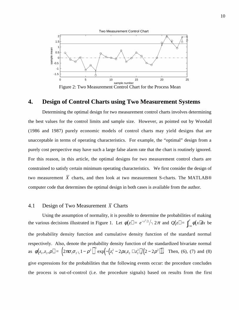
simplification that c1 = gives: r n1 = 2.80, c n2 = 2.92, with n = 5.26 for a relative cost of

5.65. These values are given approximately on Figure 3. In this optimal solution the values for

r1 and c2 are almost equal. From an implementation perspective setting r1 and c2 equal is

desirable since it simplifies the resulting control chart as will be shown. With the additional

constraint that r1 = c2 , the optimal solution to (9) is: r n1 = c n2 = 2.89, n = 5.36 with a

corresponding cost of 5.67. For implementation the sample size is rounded off to five. Thus, the

control limits r1 and c2 are set at ±1.3. The measurement costs associated with this plan are

around 10% less than the measurement costs associated with the current plan that uses only the

first measurement device, and around 80% less than the cost associated with using only the

CMM machine.

Figure 2 gives an example of the resulting two measurement X control chart. On the

chart the sample averages based on the first measurement device are shown with an “o”, while

9

the sample average of the combined first and second measurements (if the second measurement

is deemed necessary) are shown with a “x”s. The extra measurement limit (± r1) for the results

from the first measurement device and control limit (±c2 ) for the combined sample are given by

the solid horizontal lines on the chart. If the sample average based on the first measurement lies

between the solid horizontal lines on the chart we conclude that the process is in-control.

Otherwise, if the initial point lies outside the extra measurement limits a second measurement of

the sample is required. Using the second measurement we calculate the combined sample

weighted average w = .01Y1+.99Y2 (based on this weighting we could use just Y2 rather than w

without much loss of power in this example). If w falls outside the solid horizontal lines we

conclude the process shows evidence of an assignable cause; otherwise the process appears to be

in-control. The dashed/dotted line denotes the center line of the control chart. In this example,

for illustration, the value 1.0 was added to all the measurements after the 19th observation to

simulate a one sigma shift in the process mean. Figure 2 shows that in the 25 measurements a

second sample was required six times, at sample numbers 7, 20, 21, 22, 24 and 25. However,

only samples 21, 22, 24 and 25 yield an out-of-control signal. In the other cases, the second

measurement of the sample suggests the process is still in-control. Of course the number of

times the second measurement was needed after observation 19 is also an indication that the

process has shifted. In this application, using two measurement control charts results in a

reduction in the measurement costs without affecting the ability of the monitoring procedure to

detect process changes.

10

0 5 10 15 20 25

-1.5

-1

-0.5

0

0.5

1

1.5

2

Two Measurement Control Chart

sam

ple

mea

n

sample number

Figure 2: Two Measurement Control Chart for the Process Mean

4. Design of Control Charts using Two Measurement Systems

Determining the optimal design for two measurement control charts involves determining

the best values for the control limits and sample size. However, as pointed out by Woodall

(1986 and 1987) purely economic models of control charts may yield designs that are

unacceptable in terms of operating characteristics. For example, the “optimal” design from a

purely cost perspective may have such a large false alarm rate that the chart is routinely ignored.

For this reason, in this article, the optimal designs for two measurement control charts are

constrained to satisfy certain minimum operating characteristics. We first consider the design of

two measurement X charts, and then look at two measurement S-charts. The MATLAB®

computer code that determines the optimal design in both cases is available from the author.

4.1 Design of Two Measurement X Charts

Using the assumption of normality, it is possible to determine the probabilities of making

the various decisions illustrated in Figure 1. Let φ z( ) = e− z 2 2 2π and Q z( ) = φ x dxz

( )−∞∫ be

the probability density function and cumulative density function of the standard normal

respectively. Also, denote the probability density function of the standardized bivariate normal

as φ z1, z2 ,ρ( ) = 2 1 2 2 21 22

1

12

1 2 22 2πσ σ ρ ρ ρ−( ) − − +( ) −( )( )−

exp z z z z . Then, (6), (7) and (8)

give expressions for the probabilities that the following events occur: the procedure concludes

the process is out-of-control (i.e. the procedure signals) based on results from the first

11

measurement; measuring the sample with the second measurement is necessary; and the

combined results from the first and second measurement devices leads to a signal.

p1 µ( ) = Pr(signal on first measurement) = Pr Y1 > c1 OR Y1 < −c1( )= 1 1 1 1 1+ − −[ ]( ) − −[ ]( )Q c Q cµ σ µ σ* * (6)

q1 µ( ) = Pr(second measurement needed) = Pr r1 < Y1 < c1 OR − r1 > Y1 > −c1( )= Q c Q r Q r Q c1 1 1 1 1 1 1 1−[ ]( ) − −[ ]( ) + − −[ ]( ) − − −[ ]( )µ σ µ σ µ σ µ σ* * * * (7)

p2 µ( ) = Pr(signal on combined measurements)

= Pr w > c2 OR w < −c2( )& r1 < Y1 < c1 OR − r1 > Y1 > −c1( )( )= φ ρ

µ σ µ σµ σ

z z dz dzw

z r c

z c w

1 2 1 2

1 1 1 1 1

2 2

, ,* *

*

,

,

( )∈ −( ) −( )[ ]∈ −∞ − −( )[ ]

∫∫ + ( )∈ −( ) −( )[ ]∈ −( ) ∞[ ]

∫∫φ ρµ σ µ σµ σ

z z dz dzw

z r c

z c w

1 2 1 2

1 1 1 1 1

2 2

, ,* *

*

,

,

φ ρµ σ µ σ

µ σ

z z dz dzw

z c r

z c w

1 2 1 2

1 1 1 1 1

2 2

, ,* *

*

,

,

( )∈ − −( ) − −( )[ ]∈ −∞ − −( )[ ]

∫∫ + ( )∈ − −( ) − −( )[ ]∈ −( ) ∞[ ]

∫∫φ ρµ σ µ σ

µ σ

z z dz dzw

z c r

z c w

1 2 1 2

1 1 1 1 1

2 2

, ,* *

*

,

,

(8)

where σ1* = σ σ2

12+( ) n , and σ w

* = σ σ σ σ σ σ σ σ212 2

22

12

22

12

22+ +( ) +( )n . Note that p1, p2

and q1 depend on the true process mean and standard deviation. Setting c1 equal to infinity

results p1 µ( ) = 0 for all µ

In this article a cost model based on measurement costs is developed. This measurement

cost model is easy to use since it requires only estimates of the fixed and variable measurement

costs for the two measurement devices. A more complex cost model that considers all the

production costs could be developed based on the general framework of Lorenzen and Vance

(1986). However, the production cost model is often difficult to apply, since costs due to false

alarms, searching for assignable causes, etc. are difficult to estimate in many applications.

The goal is to minimize the measurement costs while maintaining the desired minimum

error rates of the procedure. Let f i and vi denote the fixed and variable measurement costs for

the ith measurement system respectively ( i = 1, 2). In our analysis, without loss of generality,

we may set v1 = 1, since the results depend only on the relative values of the measurement costs.

In addition, to restrict the possibilities somewhat, the fixed cost associated with the first

12

measurement device is set to zero, i.e. f1 = 0. This restriction is justified because typically the

first measurement device is very easy and quick to use, and would not require much setup time

or expense. Then, the measurement cost per sample is n f v n q+ +( ) ( )2 2 1 µ . The best choice for

the sampling interval must be determined through some other criterion, such as the production

schedule. There are a number of ways to define an objective function using the measurement

costs. Since the process will (hopefully) spend most of its time in-control we minimize the in-

control measurement costs. Using this formulation, the optimal design of the control chart using

two measurement devices is determined by finding the design parameters that

minimize n f v n q+ +( ) ( )2 2 1 0 (9)

subject to α = p1 0( ) + p2 0( ) .0027 and β = 1– p p1 22 2( ) + ( ) .0705

where α is the false alarm rate, i.e. the probability the chart signals when the process mean is in-

control, and 1–β is the power the probability the chart signals when the process mean shifts to

µ1 = ±2. These particular choices for maximum false alarm rate and minimum power to detect

two sigma shifts in the mean are based on at least matching the operating characteristics of a

Shewhart X chart with samples of size five.

Optimal values for the design parameters c1, c2 , r1 and n, that satisfy (9) can be

determined using a constrained minimization approach such as applying the Kuhn-Tucker

conditions. This solution approach was implemented using the routine “constr” in the

optimization toolbox of MATLAB®.

Figures 3 and 4 show the optimal design parameters for two measurement charts that

satisfy (9) for different measurement cost parameters when setting c1 equal to infinity. Figure 3

gives results when the second measurement device also has no fixed costs, while Figure 4

considers the situation where the fixed cost associated with the second measurement device is

relatively large. Figures 3 and 4 may be used to determine the design parameter values that are

approximately optimal for two measurement X charts in terms of in-control measurement costs.

For measurement costs in between those given, interpolation can be used to determine reasonable

13

control limit values. In practice, the sample size, n, must be rounded off to the nearest integer

value. Rounding off the sample size effects the power of the control chart, but has no effect on

the false alarm rate of the procedure. Of course, rounding down the sample size decreases the

procedure’s power, while rounding up increases the power.

Figures 3 and 4 each consist of four subplots that show contour plots of the optimal

design parameters: r n1 , c n2 , and n as a function of σ1 and σ2, the variability inherent in the

two measurement devices. Each subplot represents four different values of ν2 , the variable

measurement cost associated with the second measurement device. Optimal values for r n1 ,

c n2 , and n in the general case where c1 is allowed to vary are very similar to those given in

Figures 3 and 4. In general, the optimal value of c1 is large and consequently does not affect the

procedure much unless there is a large shift in the process mean.

14

v2 = 1

0.5 1 1.50

0.1

0.2

0.3

0.4

0.5

22.2

2.42.6

2.82.9

r1*sqrt(n)

σ1

σ 2

0.5 1 1.50

0.1

0.2

0.3

0.4

0.5

2.95

33.05

3.1

3.2

c2*sqrt(n)

σ1

σ 2

0.5 1 1.50

0.1

0.2

0.3

0.4

0.5

5.5

6

n

σ1

σ 2

v2 = 2

0.5 1 1.50

0.1

0.2

0.3

0.4

0.5

2.4

2.5

2.6

2.72.8

r1*sqrt(n)

σ1

σ 2

0.5 1 1.50

0.1

0.2

0.3

0.4

0.5

2.9

2.95

3

3.05

3.1

c2*sqrt(n)

σ1

σ 2

0.5 1 1.50

0.1

0.2

0.3

0.4

0.5

5.5

6 7

n

σ1

σ 2

v2 = 4

0.5 1 1.50

0.1

0.2

0.3

0.4

0.5

2.8

2.9

3

33

r1*sqrt(n)

σ1

σ 2

0.5 1 1.50

0.1

0.2

0.3

0.4

0.5

2.92.95

3

3.05

3.1

c2*sqrt(n)

σ1

σ 2

0.5 1 1.50

0.1

0.2

0.3

0.4

0.5

5.5

67

8n

σ1

σ 2

v2 = 6

0.5 1 1.50

0.1

0.2

0.3

0.4

0.5

2.8

2.9

3 3

3.23

r1*sqrt(n)

σ1

σ 2

0.5 1 1.50

0.1

0.2

0.3

0.4

0.5

2.82.9

233.053.1

c2*sqrt(n)

σ1

σ 2

0.5 1 1.50

0.1

0.2

0.3

0.4

0.5

5.5

67

8

9n

σ1

σ 2

Figure 3: Contour Plots of the Design Parameters for the No Fixed Cost Casef1 = 0, v1 = 1, f 2 = 0

15

v2 = 1

0.5 1 1.50

0.1

0.2

0.3

0.4

0.5

2.7

2.8

2.9

r1*sqrt(n)

σ1

σ 2

0.5 1 1.50

0.1

0.2

0.3

0.4

0.5

2.9

2.95

3

3.05 3.1

c2*sqrt(n)

σ1

σ 2

0.5 1 1.50

0.1

0.2

0.3

0.4

0.5

5.5

6

7

n

σ1

σ 2

v2 = 2

0.5 1 1.50

0.1

0.2

0.3

0.4

0.5

2.8

2.9

33

r1*sqrt(n)

σ1

σ 2

0.5 1 1.50

0.1

0.2

0.3

0.4

0.5

2.92.95

33.05

3.1

c2*sqrt(n)

σ1

σ 2

0.5 1 1.50

0.1

0.2

0.3

0.4

0.5

5.5

67

8n

σ1

σ 2

v2 = 4

0.5 1 1.50

0.1

0.2

0.3

0.4

0.5

2.8

2.9

3

3

3.1

3.2

3

r1*sqrt(n)

σ1

σ 2

0.5 1 1.50

0.1

0.2

0.3

0.4

0.5

2.8

2.92.953

3.05

3.1c

2*sqrt(n)

σ1

σ 2

0.5 1 1.50

0.1

0.2

0.3

0.4

0.5

5.5

6

7

8

9n

σ1

σ 2

v2 = 6

0.5 1 1.50

0.1

0.2

0.3

0.4

0.5

2.9

3

3.2

3.4

r1*sqrt(n)

σ1

σ 2

0.5 1 1.50

0.1

0.2

0.3

0.4

0.5

2.7

2.8

2.9

2.95

3

3.05

3.1c

2*sqrt(n)

σ1

σ 2

0.5 1 1.50

0.1

0.2

0.3

0.4

0.5

5.5

6

7

8

9n

σ1

σ 2

Figure 4: Contour Plots of the Design Parameters for the Large Fixed Cost Casef1 = 0, v1 = 1, f 2 = 10

16

Figures 3 and 4 suggest that the parameters r n1 and c n2 are the most sensitive to

changes in the variability of the measurement devices. In general, when the measurement costs

of the two measurement devices are comparable, as the first measurement device becomes more

variable ( σ1 increases), n increases, while r n1 decreases. This result makes sense since it

means we rely more on the second measurement device when the first device is less precise.

Conversely as the second measurement device becomes more variable (σ2 increases), c n2 and

n increase while r n1 increases marginally, since we rely more on the first measurement device.

v2 = 1 v2 = 4

0.5 1 1.50

0.1

0.2

0.3

0.4

0.50.05

0.1

0.15

0.2

0.25

Pr(2nd measurement needed in-control)

σ1

0.5 1 1.50

0.1

0.2

0.3

0.4

0.5

0.025

0.05

0.075

0.1

Pr(2nd measurement needed in-control)

σ1

Figure 5: Contour Plots of the Probability the Second Measurement is RequiredProcess in-control, f1 = 0, v1 = 1, f 2 = 0

Now consider the case where the second measurement device is expensive ( f 2 or ν2

large). As the second measurement device becomes less reliable ( σ2 increases), again we

observe that c n2 increases while n and r n1 increase marginally which makes sense.

However, the pattern appears to be counterintuitive when the first measurement device becomes

less reliable ( σ1 increases) since n and c n2 decrease marginally, but r n1 increases! Does

this mean that we rely more heavily on the inaccurate first measurement device? Looking more

closely, this apparent contradiction disappears. As σ1 increases the optimal r n1 also increases,

but this does not mean that the decisions are more likely to be based on only the first

measurement device. When the accuracy of a measurement device is poor we expect to observe

large deviations from the actual value. Thus, the observed increase in r n1 is only taking this

into account. Consider Figure 5 which shows contours of the probability the second

17

measurement is needed in the two cases: f 2 = 0 and ν2 = 1 or 4. The plots in Figure 5 show

clearly that as the first measurement device becomes less accurate we rely on it less even though,

as shown in Figure 3, r n1 increases.

We may also compare the performance of using two measurement charts with traditional

X using only one of the measurement systems. Figure 6 shows the percent reduction in

measurement costs attainable through the use of the both measurement systems as compared

with the best of the two individual measurement systems. In the case where ν2 equals 2, the

dotted line shows the boundary between where using each individual measurement system is

preferred. To the right of the dotted line (where the measurement variability of the first

measurement system is large) the second measurement system is preferred. When ν2 equals 4

and 6, the first measurement devices on its own is preferred over the second measurement device

over the whole range of the plot.

ν2 = 2 ν2 = 4 ν2 = 6

0.5 1 1.50.05

0.1

0.15

0.2

0.25

0.3

0.35

0.4

0.45

0.5 5

10

20

2

30

30

σ2

σ10.5 1 1.5

0.05

0.1

0.15

0.2

0.25

0.3

0.35

0.4

0.45

0.55

10

20

30

σ2

σ1

0.5 1 1.50.05

0.1

0.15

0.2

0.25

0.3

0.35

0.4

0.45

0.5

5

10

20

σ 2

σ1

Figure 6: Contours plots showing the percent reduction in in-control measurement costspossible using the two measurement X control chart

4.2 Design of Two Measurement S-Charts

Now consider deriving the optimal two measurement control chart to detect increases in

the process variability. Mathematically, the optimal two measurement S-chart that minimizes in-

control measurement costs is determined by finding the control limits d1 and dw that

minimize n v nps+ ( )2 1 1 (10)

subject to ps 1( ) .001 and ps 2( ) ≥ .33

18

where ps1 1( ) = Pr s d1 1 1≥ =( )σ = 1 1 112

12

12− − +( )( )−χ σn d n( ) and ps σ( ) equals the probability

the two measurement S-chart signals, i.e. ps σ( )= Pr ,s d s dw w> >( )1 1 σ . χn x− ( )12 is the

cumulative density function of a central chi-squared distribution with n-1 degrees of freedom.

Using results presented in the appendix we may accurately approximate ps σ( ) for any given

actual process standard deviation. The choice of .33 is based on the power possible using a

traditional S-chart with no measurement error and samples of size five that has a false alarm rate

of .001.

Figure 7 shows the expected percent decrease in measurement costs that result when

using the optimal two measurement S-chart rather than the lowest cost traditional S-chart based

on only one of the measurement systems. When ν2 = 1, i.e. both measurement systems are

equally expensive, using just the more accurate measurement device is always preferred, and it is

not beneficial to use the two measurement system approach. Figure 7 suggests that large

potential savings in measurement costs are possible using the two measurement approach to

detect increases in process variability.

ν2 = 2 ν2 = 4 ν2 = 6

0.5 1 1.50.05

0.1

0.15

0.2

0.25

0.3

0.35

0.4

0.45

0.5

5

10

15

20

30

30

40

40

σ2

σ1 0.5 1 1.5

0.05

0.1

0.15

0.2

0.25

0.3

0.35

0.4

0.45

0.5

5

10

15

20

30

40

50

σ2

σ1 0.5 1 1.5

0.05

0.1

0.15

0.2

0.25

0.3

0.35

0.4

0.45

0.5

5

10 15

20

30

40

50

60

σ2

σ1

Figure 7: Percentage decrease in in-control measurement costs possible with twomeasurement S-chart, assume f2 = 0

In practice, a process is typically monitored using both an X and S-charts. Thus, from an

implementation perspective using the same sample size for both charts is highly desirable. For

two measurement charts, since typically detecting changes in the process mean is a higher

priority we use the sample size suggested by the optimal two measurement X chart. Solving

19

(10) shows that the optimal sample size for the two measurement S-chart is usually smaller than

the sample size suggested for the two measurement X chart. As a result, by using the larger

sample size the resulting two measurement S-chart will have better than the minimum defined

operating characteristics.

Deriving the best values for n, d1 and dw from (10) we could prepare plots similar to

those in Figures 3 and 4. However, to simplify the design we consider an approximation. Based

on the range of typical values for measurement costs and the measurement variability, and

assuming f2 = 0, we obtain using regression analysis the following approximations for the

optimal control limits:

d̂1 = 1 94 0 18 0 28 031 12

2. . . .− + +σ σ ν , and (11)

d̂w = 2 7 0 11 0 22 01 0 271 2 2 1. . . . . ˆ− + − −σ σ ν d .

These approximately optimal limits give good results over the range of typical

measurement variability.

5. Implementation Issues

An alternative approach to process monitoring in this context is to use a second sample

that is different than the first sample; i.e. take a completely new sample rather than measuring the

first sample again. This approach is of course a necessary if the testing is destructive, but it leads

to increased sampling costs as well as difficulties in obtaining a new independent sample in a

timely manner due to autocorrelation in the process. However, if these sampling concerns can be

overcome, the advantage of using an additional sample is that more information about the true

nature of the process is available in two independent samples than in measuring the same sample

twice. If feasible, taking a new independent sample would be preferred, however, in many cases

it is not possible in a timely manner.

In a similar vein, we may consider situations where repeated measurements with a single

measurement system are feasible. If repeated independent measurements are possible then, by

20

averaging the results, we would be able to reduce the measurement variability by a factor of n .

If the measurements are very inexpensive then repeated independent measurement with one

device will eventually yield (using enough measurements) a measurement variability so small

that it may be ignored. Alternately, we could apply the methodology developed in this article

where we consider the second measurement to be simply the results of repeated measurements

on the units with the first measurement device. If repeated inexpensive independent

measurements using the first measurement device are possible using those measurements would

be the preferred approach. However, this approach will only work if we can obtain repeated

independent measurements of the units which is often not the case.

6. Summary

This article develops a measurement cost model that can be used to determine an optimal

process monitoring control chart that utilizes two measurement devices. It is assumed that the

first measurement device is fast and cheap, but relatively inaccurate, while the second

measurement device is more accurate, but also more costly. The proposed monitoring procedure

may be thought of as an adaptive monitoring method that provides a reasonable way to

compromise between measurement cost and accuracy.

Appendix

Using the notation of the article, A = y y y y w w

y y w w w w

ii

n

i ii

n

i ii

n

ii

n

1 1

2

1 1 11

1 11

2

1

−( ) −( ) −( )−( ) −( ) −( )

= =

= =

∑ ∑∑ ∑

,

, has a

central Wishart distribution with n-1 degrees of freedom and covariance matrix given by

Σ = σ σ σ σ

σ σ σ σ σ σ σ

212 2

12

212 2 2

12 2 2

22 21 2 1

+ +

+ +( ) + −( ) +( ) + −( )

,

,

k

k k k k k (Arnold, 1988). Denoting the

21

elements of the matrix A as aij it can be shown that Pr ,0 011 1 11 22 2 22≤ ≤ ∑ ≤ ≤ ∑( )a c a c =

1

1 2 1 2 11 2

2 11 2

2 1

2 1 22

12

0

22

−( )−( )( ) + −( )( ) +( ) + −( )

−( )

+ −( )

−( )

−( )

≥∑

ρ ρρ ρ

nj

jn j n jI j n

cI j n

c

Γ Γ Γ, , ,

where ∑ij is an element of the covariance matrix, ρ = ∑ ∑ ∑12 11 22 is correlation coefficient,

Γ x( ) is the gamma function, and I d g,( )= t e dtd tg − −∫ 1

0, is the incomplete Gamma function. This

infinite sum converges quickly unless ρ is very close to one (or minus one).

Acknowledgements

The author would like to thank Jock Mackay for useful discussions, and Greg Bennett for

the derivation presented in the Appendix. In addition, suggestions from a number of referees, an

associate editor, and the editor, substantially improved the article.

References

Arnold, S.F. (1988), “Wishart Distribution,’ in the Encyclopedia of Statistical Sciences, Kotz S.

and Johnson, N. editors, John Wiley and Sons, New York.

Croasdale, R. (1974), “Control charts for a double-sampling scheme based on average

production run lengths,” International Journal of Production Research, 12, 585-592.

Daudin, J.J. (1992), “Double Sampling X Charts,” Journal of Quality Technology, 24, 78-87.

Lorenzen, T.J. and Vance, L.C. (1986), “The Economic Design of Control Charts: A Unified

Approach,” Technometrics, 28, 3-10.

Woodall, W.H. (1986), “Weaknesses of the Economic Design of Control Charts,”

Technometrics, 28, 408-409.

Woodall, W.H. (1987), “Conflicts Between Deming’s Philosophy and the Economic Design of

Control Charts,” in Frontiers in Statistical Quality Control 3 edited by H.J. Lenz, G.B.

Wetherill, and P.Th. Wilrich, Physica-Verlag, Heidelberg.