statistical properties of - uzh

STATISTICAL PROPERTIES OF ART PRICING MODELS

Course: Executive Master in Art Market Studies, University of Zurich

Master Thesis

Supervisors: Prof. Dr. Alexander Wagner and Dr. Nicolas Galley

Author: Res Urech

Contact: [email protected]

Date: 20 May 2013

(This version 14 October 2014)

Statistical Properties of Art Pricing Models /69

State of Authorship: I hereby certify that this Master Thesis has been composed by myself and describes

my own work, unless otherwise acknowledged in the text. All references and verbatim

extracts have been quoted, and all sources of information have been specifically

acknowledged. This Master Thesis has not been accepted in any previous application

for a degree.

Zurich, 20 May 2013

Acknowledgements: I would like to thank my supervisor, Prof. Dr. Alexander Wagner, for giving me the

opportunity to apply econometric methods to art pricing models under his guidance.

I am most indebted to him for his constructive feedback and the time he took for

discussions even during stressful times.

I also give thanks to my second supervisor, Dr. Nicolas Galley, Director of the

EMAMS Programme, for his support and patience with demanding students during

the whole two years of the Master Programme.

During the EMAMS lectures on Valuation and at the Deloitte Conference in

Maastricht in March 2013 I had the opportunity to discuss topics with Fabian Bocart,

Quantitative Research Director at Tutela Capital, which go beyond this work. I am

indebted to him that he shared his views with me. Part of the discussion with him is

covered in the section on possible extensions at the end of my thesis.

I am grateful to Annemarie Kallen for the very careful proofreading not only of the

Master Thesis but also of all the Written Assignments during the Master Programme.

I give my warmest thanks go to our son David who typed all the data on the

drawings and paintings of Ed Ruscha from the Artprice website into an Excel sheet.

He did this cumbersome task with patience and a keen mind (“An estimate of

GBP 500’000’000 is not meaningful!”). Any remaining errors are completely mine.


Table of Content 1 Introduction ............................................................................................................... 4

2 Index construction ..................................................................................................... 8

2.1 Hedonic regression ........................................................................................... 9

2.2 Repeat-sales regression ................................................................................. 11

3 Price indices ............................................................................................................ 12

3.1 Artprice ............................................................................................................ 12

3.2 artnet ............................................................................................................... 15

3.3 Art Market Research ....................................................................................... 19

4 Pricing models ........................................................................................................ 22

4.1 Skate’s art asset pricing model ....................................................................... 22

4.2 Art pricing in the determination of the expected loss for art backed loans ...... 25

4.3 Artworks as collateral values in bank loans ..................................................... 34

5 Conclusion .............................................................................................................. 43

5.1 Art Indices ....................................................................................................... 43

5.2 Art Pricing Models ........................................................................................... 43

5.3 Extensions ....................................................................................................... 45

Bibliography ............................................................................................................... 48

Appendix .................................................................................................................... 52

Appendix A: Comparison of Ed Ruscha’s photographs to paintings and

drawings at auctions .............................................................................................. 52

Appendix B: Remark on logarithmic properties ..................................................... 61

Appendix C: Rating system of the Artprice Indicator® .......................................... 61

Appendix D: Removal of autocorrelation in time series ......................................... 62

Appendix E.1: Expected loss for art backed loans ................................................ 65

Appendix E.2: Artworks as collateral values in bank loans ................................... 66

Appendix F: Statistical tests .................................................................................. 66

Appendix G: Estimate of mean and standard deviation for a truncated normal

distribution ............................................................................................................. 68

1 Introduction


1 Introduction

In November 2012 the painting No. 1 (Royal Red and Blue) of the American painter

Mark Rothko was auctioned at Sotheby’s in New York (fig.1). It is a wonderful

painting that had an exciting pre-sale estimate range of USD 35 to 50 million, which is

not at all explainable with any materiality argument. The price seems to be detached

from the tangible ingredients, as long as immaterial ingredients like the artist’s

reputation or the importance of the period in the œuvre of the artist are not valued.

The painting has been marketed with its uniqueness in the artist’s development and

career, with its perfect provenance and “aura”.1 The latter is the most difficult

component to explain and document, and its perception may change over time, since

it is related to the zeitgeist. The auction of Mark Rothko’s painting was a success; the

work was sold for USD 67 million, one third over the upper estimate. The painting

was recorded in Skate’s Top 5000 database at USD 75’122’496 including the buyer’s

premium and stands at position 13 of the 5’000 most expensive works recorded at

auction.2 The difference between the hammer price of USD 67 million and the price

including the buyer’s premium corresponds to the fee Sotheby’s earned. Additionally

there is also a seller’s premium for the auction house of a few percentages, which is

however negotiable for expensive works such as No. 1 (Royal Red and Blue).

Without having to do great math it is obvious that the marketing campaign paid-off.

Gertrude Stein said, “A work of art has either a value or a price”.3 In her

terminology the value of the work is related to the perception by knowledgeable

persons in art history, i.e. art critics, curators, academic researchers in art history and

knowledgeable art collectors. The price, on the other hand, is the exchange value of

a good between two parties. It is real, and most often related to a money transfer.

The two concepts of value and price may indeed be different, but it is doubtful

whether they are completely detached: A highly valued work of art is costly, but

whether a work traded at a high price has a corresponding art historical valuation is

more questionable. Most of the living artists have to undergo the litmus test of their

actual valuation.

In this thesis we will concentrate on the price and the pricing of artworks by

means of statistical methods. Often assumptions have to be made concerning the

rules of price developments. These assumptions will be tested on a limited set of 1 See the video from Sotheby’s website, www.sothebys.com/en/auctions/2012/contemporary-art-evening-auction-n08900/videos.html, last access on 20.1.2013. 2 www.skatepress.com, last access on 20.1.2013. 3 Gertrude Stein (1874–1946) was an American writer, poet and art collector; citation from Alicia Legg (Ed.), Sol LeWitt, Museum of Modern Art, New York, 1978, p.164.

1 Introduction


publicly available data. In the following, artworks will be regarded as part of a

homogeneous portfolio. Although, we know that apart from prints and photography

artworks are unique and heterogeneous.

Figure 1 Mark Rothko, No. 1 (Royal Red and Blue), 1954, oil on canvas; 288.9 x 171.5 cm, from: http://qzprod.files.wordpress.com/2012/11/mark-rothko_s-1954-no-1-royal-red-and-blue-1.jpg?w=1024&h=1760, last access on 15.4.2013.

1 Introduction


The thesis starts with an introduction in Chapter 2 to the methods of the art price

index construction. In Chapter 3 we discuss different commercially available price

indices. We compare two price estimates for a single artwork by Ed Ruscha to the

pre-sale estimates and the realised hammer price at auction. Neither of the indices

has made a convincing proposal for the realised price paid by the buyer.

For a third index we confirm that the time series is smoothed by construction. By a

de-smoothing methodology originally applied to real estate and hedge fund returns

we show that the underlying volatility is substantially higher than the reported

standard deviation.

The main take-away from these results is the reminder to be careful when using

an art price index without knowing the underlying methodology. Knowledge of the

methodology allows to judge on the outcome and to decide how far it should be

included in any expectation or decision.

In Chapter 4 the distributions of different pricing models are investigated: Skate

Art Market Research’s Art Asset Pricing Model (AAPM), the pricing of Campbell and

Wiehenkamp (2009) in the determination of the expected loss for art backed loans

and the pricing of artworks by McAndrew and Thompson (2007) as collateral value.

We transform Skate’s art asset pricing model into the form of a hedonic regression

and find that the expected price movement over time is the consumer price inflation.

The model also contains an irrational premium which reflects the buyer’s willingness

to over- or underpay the fair value of the artwork. This premium may or may not

occur, and is therefore not predictable. In the hedonic regression we assign it to the

idiosyncratic error term.

In the other two pricing models we put the focus on the price distribution. We

apply the distribution used in Campbell and Wiehenkamp (2009) to the repeat-sales

data from Skate’s Art Market Research and find that although the fitted function is

well shaped and passes three statistical tests to a high degree, the data is biased due

to the index construction and contains too few negative returns.

Skate’s Art Market Research is a consultancy company among many. However,

the company is exceptional compared to other commercial art service firms in the

sense that it makes data on sold artworks available on its website for free and

downloadable in Excel-format.4 Throughout the academic literature the most valuable

good is the data set each researcher has gathered for his or her studies. The

individual results can hardly be checked or confirmed by others with the same data

since they are treated confidentially and proprietarily. Thus it may happen that,

4 cf. note 2.

1 Introduction


depending on the data, different findings occur with similar methods for the same

question under investigation. As an example we name the Underperformance of

Masterpieces. Mei and Moses (2002) found that the future excess price of master-

pieces, i.e. expensive artworks, is lower than for the other artworks, whereas

Renneboog and Spaenjers (2013) found a higher performance for higher priced

artworks compared to others.5 We will come back to this specific topic in Chapter 4.2.

Finally, the methodology of McAndrew and Thompson (2007) considers the pre-

sale estimate of the auction house (or from any other evaluator) as true fair value and

attempts to estimate the price distribution based on the ratio of the hammer price to

the pre-sale auction house estimate, and to include the bought-ins. Bought-ins are

lots that are not sold at auctions due to a reserve price set by the seller, and the work

is “bought in-house” by the auctioneer. The highest bid remains unpublished, the

price estimate and the tag “Not sold” are the only publicly available information on

bought-ins. This incomplete information does not correspond to their importance for

auction houses and collectors:

1. In approximately 20% of the cases a sale takes place immediately after the

auction with the price again negotiated between the seller, the auction house

and the buyer. Often this sale is not published.

2. An unsold artwork at auction is banned from the art market for a quite a while

or can only be offered at a lower price.6 It is referred to as burned.

3. The reputation of the auction houses depends on the sale rate, i.e. the

percentage of works sold compared to the total number of lots offered: The

higher the sale rate the higher the confidence of potential consignors that the

auction house is able to sell the works at the estimated prices.

It is therefore worthwhile to consider bought-ins in the distribution of auction

prices. We apply the model of McAndrew and Thompson (2007) to the auction results

for drawings, paintings and photographs of Ed Ruscha and find that the model fits

well to this data sample. We determine a distribution for the bought-ins which we did

not find in this explicit form in the literature.

Chapter 5 contains the conclusion and lists possible extensions related to the

topics discussed in the main text.

5 For a review of earlier studies see Ashenfelter and Graddy (2003). 6 For a study on the future value of unsold works at auction see Beggs and Graddy (2008).

2 Index construction



The methods used for the construction of the price development of an artwork rely on

principles for the estimate of market prices of heterogeneous goods. Real estate

valuation is maybe the most prominent example and a forerunner for the application

of the index construction to artworks. Often, researchers that work in the field of real

estate valuation also apply the same methodology to art pricing.7 The price

construction of heterogeneous goods usually involves the characteristics of the

individual items and the development over time.

The characteristics contain measurable and descriptive attributes of the artwork,

such as artist, technique, subject, date or period of creation and dimensions. It is

usually assumed that the characteristics do not change and stay the same over time.

The provenance can also be an important factor. Especially for potentially looted art

and for flight art during the Second World War, the complete owner’s history is crucial

information. Provenance is less important for contemporary art, although the glory of

a prominent owner is used in the marketing when a work or a collection comes to

auction.8

The time development is related to changes in the economic environment, to the

availability of collectors and their capability and willingness to invest in art.

Anecdotally, sales at auction are driven by the three D’s: Death, divorce and debts,

i.e. need for money. The first two incidents can reasonably be assumed to be

independent from economic environmental changes, whereas outstanding debts

often go with missing liquidity, e.g. in a financial crisis. Mostly a liquidity crunch does

hit a broader group of wealthy people who may then be forced to sell artworks or at

least have a restricted capability to buy more artworks. As a consequence the prices

drop without any change in the qualitative aspects of the works. With excess money

available, the mechanism goes in the other direction and prices rise. Independent

from the economic situation, a repositioning of the artist in the art historical context

also influences the price development.

The two main methods commonly used for index construction are hedonic

regression (HR) and repeat-sales regression (RSR).

7 See e.g. William N. Goetzmann, http://www.brg-expert.com/media/bio/213_Goetzmann_William_CV.pdf, last access on 3.3.2013. 8 See the magazine for the auction of the Yves Saint Laurent and Pierre Bergé art collection at Christie’s on 23–25 February 2009, http://www.christies.com/images/email/jan09_ysl_en/ysl_feb09.pdf, last access on 3.3.2013.



2.1 Hedonic regression

Hedonic regression controls the characteristics of the objects, and the residual is then

said to be the characteristic-free contribution to form a price index.9 This regression

can be as simple as the distinction of the artist, size of the artwork and number of

editions (for photography), or can be run over almost 100 variables.10 Although the

latter likely gives a higher degree of numerical precision than the former, the

interpretation is not straightforward and becomes less clear when more variables are

considered. The method needs price records and as precise information on the

artwork as possible. Usually this means that only auction data can be considered,

since transactions involving galleries which are mostly active on the primary market

and art dealers for the secondary market are rarely available publicly. It is estimated

that auctions cover roughly 50% of all the transactions in the art market.11 Therefore

hedonic regressions serve as a proxy for the art market but do not represent the

entire market.

Mathematically, hedonic regression for an observed price itP of an artwork i at

time t can be expressed as

ittiitit ppPp )ln( , (2.1)

where )ln( itP is the natural logarithm of itP , ip is the contribution from the unique

character of the artwork, assumed to be fixed over time, and therefore without time

index t . tp stands for the contribution to the aggregate index of price movements

valid for all different artworks considered, and it is the work- and time-specific error

term which is assumed to have zero mean, i.e. it vanishes on average.12

The term ip is represented as

iii xp ,

where ix contains the information on the characteristics of the artwork i , is the

universal parameter to be fitted to the data and i is again an error term. We obtain

ittiit pxp ~ ,

9 Ginsburgh et al. (2006), p. 953. 10 Example for the first variant: For Ed Ruscha with 545 auction results from 1987 to 2012, the descriptive statistic with the three variables: Number of editions for photographs, size and an art market index can explain up to 65% of the auction prices. See Appendix A. Example for the second variant: For 32 Western artists with 3’291 observations from 1992 to 2007, the descriptive statistic with 96 variables can explain 80% of the prices. See Gawrisch (2008). 11 McAndrew (2012), p. 55. 12 See Appendix B for a remark on the choice of the natural logarithm as price index function.



with itiit ~ . For later use we have a closer look at tp , which results from the

time series of all sales of the involved artworks and can be estimated from the

average of the realised prices at time t after the deduction of the characteristics,13

tn

iiit

tt xp

np

1

1ˆ , (2.2)

where tp̂ is an estimator for tp , and tn is the number of sold works at time t .14 It

represents a price component that is free of the characteristics, unspecific for any

artwork that takes part in the regression. Nevertheless, this price component contains

a selection bias due to the fact that only sold works are taken into account. The

bought-ins are left aside. In a study on auction data of French Impressionists

McAndrew and Thompson (2007) found a bought-in rate of 30%. In Chapter 4.3 we

will see how they attempted to overcome this shortcoming in their pricing model.

The illustrative representation in eq.(2.2) assumes that the ordinary least square

(OLS) estimator can be used. For cases where the OLS estimator is inappropriate

more tedious approaches are needed, see e.g. Ginsburgh et al. (2006) and

Goetzmann et al. (2010b).

Also noteworthy is the effect of adding a new sale jsp to the regression. Most

likely, the regression will lead to other coefficients ~ for the characteristics due to the

heterogeneity of the artworks. From eq.(2.1) it is obvious that tp̂ will change although

the artwork j is sold at time ts . Due to the change ~ the common price

development changes in every time period. This effect is called revision bias and may

also occur in the case of a re-classification of a work, e.g. from Contemporary Art to

Post-Modernism Art, or if new information concerning the chain of owner is included.

Revision bias matters in case art price indices are published.15 Due to the

inclusion of fresh auction results the price history will be changed. In Chapter 3.2 we

will have a look how artnet, an art consultant company and auction data provider,

deals with this problem.16

A way to overcome the shortcoming of the revision bias, at least partly, is the

method of repeat-sales regression.

13 Ginsburgh et al. (2006). 14 For practical use, the time t stands usually for a time period of one year instead for a single point in time. The one-year period will be assumed in the analysis unless stated differently. 15 The corresponding issue for real estate is studied in Deng and Quigley (2008). 16 www.artnet.com, last access on 1.3.2013.



2.2 Repeat-sales regression

In this regression only artworks are considered that have been sold at least twice. We

look for the return between the two sales. Be the work i sold at time t as well as

again later on at time T . From eq.(2.1) we have

itiTtTitiT pppp ,

where the characteristics related term ip vanishes since we assume that the

character of the artwork does not change over time. We have therefore a

characteristic free set of equations, apart from the residuals, over all holding periods

of distinct artworks. The equation is then written as17

T

tkikkiitiT rpp

1 ,

with ir the return from the holding period tT of artwork i and k the universal

price movement in period k during the holding period. The determination of the esti-

mator ̂ goes along the same lines as for tp̂ in the hedonic regression in eq.(2.1).

The selection bias increases with repeat-sales regression since the fraction of

included trades is reduced significantly compared to the method of hedonic

regression. Goetzmann et al. (2010b) found 1349 resales out of 6661 works sold at

least once. Skate’s Top 5000 database contains 869 resales. The former yields a

resale ratio of 20% out of all works considered, where we do not know the exact

number of transactions. The latter has a resale ratio of 17% out of all trades.

The revision bias is still inherent in the approach, but does not affect the whole time

series as it does in hedonic regression. In case a new resale is included, the price

movement changes for the holding period of the newly added trade.

The holding period shows considerable differences depending on the data sample

used. In Mei and Moses (2002) the holding period is indicated as “on average 28

years”.18 Their data sample starts in 1875 and lasted until 2000 by the time of

publication. The Skate's Annual Art Investment Report for 2012 shows as an average

holding period a substantially lower holding period: 8.4 and 9.3 years for resales in

2011 and 2012 respectively.19 The report covers the resales from the believed 5’000

most expensive artworks and starts in 1989 with the first resale. A calculation over all

the resales gives an average holding period of 8.5 years. Therefore, the addition of

an actual resale is expected to change return history in the repeat-sales index of the

last 10 years. 17 Mei and Moses (2002). 18 Ibid., p. 1657. 19 Skate’s Art Market Research, Annual Art Investment Report 2012, Part 1, p. 7.

3 Price indices


3 Price indices

In this Chapter we have a look at three commercially available indices. We discuss

the methodologies and compare two price estimates for a single artwork of Ed

Ruscha to the pre-sale estimates and the realised hammer price at auction. For a

third index we confirm that the series is smoothed and apply a de-smoothing

methodology to determine the underlying volatility.

3.1 Artprice

In this section we show that Artprice’s indicator for a single artwork by Ed Ruscha

fails to predict the auction price realised in March 2013 even though it shows a large

increase since November 2000.

Artprice is a publicly listed French company under the major control of Thierry

Ehrmann.20 It had a market capitalisation of around USD 260 million as of

31 December 2012 and is the second largest publicly traded art service company

(behind Sotheby’s).21 It provides art services such as research, analyses and access

to their proprietary auction price database. In case enough data for an artist is

available, Artprice applies its Artprice Indicator®.22 The goal of the indicator is to give

a present value for a work, which has been auctioned. The indicative price comes

with a rating system for the quality of the estimate.

The exact price mechanism is not published. The methodology papers tell that

different index types are used: The highest precision includes all characteristics in a

hedonic regression and needs five auction results per year which match the required

criteria. In case of poor data the procedure is then reduced step by step. The lowest

level still relies on a single artist’s works; no aggregation of different artists is applied.

The characteristics used are signature, size, medium, period the works date from,

material and technique used and the place of sales. In case information on the

characteristics is missing, the regression is restricted to the medium. If there is still

not sufficient information available, all media are included from the artist except the

prints, and in a last step, prints are also considered. The procedure may be changed

from year to year depending on the data available, which is then reflected in the

rating system. It is explicitly mentioned that some features are not included, namely:

State of preservation, origin, subject and framing.

Depending on the applied procedure, the indices are named differently: Artwork

Price Index, Medium Price Index or Artist Price Index. This differentiation is

20 www.artprice.com, last access on 24.2.2013 21 Skate’s Art Market Research, Annual Art Investment Report 2012, Part 2, p. 27. 22 Artprice Indicator Methodology, web.artprice.com/indicator/howto?l=en, last access on 20.2.2013.

3 Price indices


considered in the rating system called degree of relevance and indicated by a system

of up to five stars. Results with less than three stars are not made available.23

The price indicator like other hedonic regression models suffers from selection

bias since only sold works are considered. However, in the artist and medium price

index development, the ratio of bought-ins to the total amount of works is shown; and

therefore can be taken qualitatively into consideration.24

As an example we take a closer look at the price indicator of the painting Anchor

Stuck in Sand (1990) from the artist Ed Ruscha (fig.2).25 The artwork was sold on

15 November 2000 for USD 60’000 with an estimate between USD 65’000 and USD

85’000 at Sotheby’s in New York. The work was offered again at auction on

5 October 2012 with an estimate between USD 700’000 and USD 900’000 at Phillips

de Pury & Company in New York. The starting bid was USD 500’000 and the painting

was not sold.26 Anchor Stuck in Sand was on offer again only five months later on

7 March 2013 for an estimate between USD 600’000 and USD 800’000, again at

Phillips in New York.

Figure 2 Ed Ruscha, Anchor Stuck in Sand, 1990, acrylic on canvas; 153 x 283.1 cm, from: http://www.liveauctioneers.com/item/11426722_ed-ruscha-anchor-stuck-in-sand-1990, last access on 1.3.2013.

23 See Appendix C for a description of the method. 24 See Figure 17 and the discussion in Chapter 5 for a possible quantitative approach. 25 An introduction to Ed Ruscha (American, born 1937) follows in Chapter 4.3.1. 26 http://www.liveauctioneers.com/item/11426722_ed-ruscha-anchor-stuck-in-sand-1990, last access on 1.3.2013.

3 Price indices


This time it was still not sold at auction, but immediately afterwards it was sold

privately for USD 550’000 including the buyer’s premium.27 Artprice calculated the

hammer price of USD 456’500.

The Artprice Indicator® for Anchor Stuck in Sand was calibrated at the end of the

year 2000 to the hammer price of USD 60’000. It increased until the end of 2012,

when the subsequent auction took place, to USD 197’287 (see fig.3). Interestingly,

the price indicator development had the highest rating until the end of 2011, and then

it broke down significantly. The indication was far below the estimates made at

auction. Even if we doubt the assumed performance in 2012 due to the lower

estimate quality, the gap between the price indication and auction estimates is large.

Figure 3 Artprice Indicator® for Ed Ruscha’s Anchor Stuck in Sand (1990). The indicator is calibrated in 2000 to the hammer price of USD 60’000. The price estimate is calculated back to 1993 and the forecast ends in 2012 at almost USD 200’000 based on auction results not specified otherwise. The stars correspond to a rating concerning the quality of the indicator.28 Table and Chart are from: www.artprice.com, last access on 1.3.2013.

27 See http://www.phillips.com/Xigen/file.ashx?path=\\diskstation\website\Media\Auction\auctionResultsFile_NY010213.pdf, last access on 28.3.2013. 28 Contrary to the statements made in the methodology paper, the maximum rating has six instead of five stars, and the index is published even with two stars only. Information from Artprice (Email from 4.3.2013): “Unfortunately we are in the middle of upgrading our Artworks Indexator, and the "star" system is right now having a little bug. We'll fix it as soon as possible”.

Year

3 Price indices


3.2 artnet

In this section we find that artnet’s grouping of comparable works to Ed Ruscha’s

Anchor Stuck in Sand (1990) is questionable, and that there are no price changes

after a sharp increase in 2001.

artnet is a publicly listed German company under the major control of Hans

Neuendorf and operationally led by his son, Jacob Pabst.29 It had a market

capitalisation of approximately USD 19 million as of 31 December 2012, much less

than Artprice’s market capitalisation.30 It is an online platform for gallery owners and

collectors buying, selling and researching artworks. For clients artnet provides access

to their proprietary auction price database and calculates indices according to the

artnet Index Methodology for approximately 75% of the sold lots recorded in the

database.31 The individual indices are finally aggregated to broader market indices,

such as the artnet C50™ Index.

The price indices are calculated by means of a mixed or hybrid model of a

hedonic regression and a repeat-sales regression, i.e. the repeat-sales regression is

a “nested case” of the hedonic regression.32 The core of the model is to extend the

repeat sale regression to sets of comparables in order to get a broader database.

Comparables consist of groups of works by a single artist and are defined by experts

based on “appraisal principles and art historical knowledge”.33 I.e. the specific

knowledge lies in the identification of the comparables and less in the methodology,

which is documented in a detailed manner. The corresponding logarithmic price of an

artwork i belonging to the comparable set s and sold at time t may be written

similar to eq.(2.1):

isttsistist pppp ,

where the price istp is corrected by the average istp of the prices from the works

belonging to the comparable set s sold at time t , and sp represents the

characteristics of the comparable set s instead of the contribution from the single

artwork i . The underlying assumption is the equivalence of the works in the

comparable set, and that the artworks within a set are priced on a similar level.

The prices are estimated on a monthly basis. In case no sale has taken place in

the current month, a zero return is assumed. If new data is added, the regression for

29 cf. note 16. 30 cf. note 21. 31 artnet Indices White Paper (Version 18 July 2012), http://www.artnet.com/analytics/reports/artnet-indices-white-paper, last access on 1.3.2013. 32 Ibid., p. 16. 33 Ibid., p. 3.

3 Price indices


the price history changes as discussed in Chapter 2.1. In order to prevent that the

past values of the indices are adjusted too often and only for small amounts, the

parameters are calculated with a confidence level. When new data is considered, the

estimated parameters of an index are compared with and without the new sale data.

If the adapted parameters lie outside the boundaries given by the confidence interval,

the index is updated. In case the estimated values are still within the previous range

of confidence, the parameters of the index are kept. The calculation of the confidence

level is explained in great detail in the methodology paper; however, the specific

confidence level that is applied in the index determination is not given.

Composite indices such as the artnet C50™ Index are adjusted once a year in

early January. For the market or sector under consideration the artists are ranked

based on the sales data over the last five years. For each year an adapted sales

volume ktV is calculated, which corrects for the outliers by taking the median instead

of the average,

ktktNktktkt NpppVkt

,,,median 21 ,

where iktp is the hammer price of the artwork i of artist k in year t and ktN is the

number of lots sold of artist k in year t . The rank of a single artist k is calculated by

using a weighted sum of the adapted volumes ktV . The weights are exponentially

decreasing backwards in time, i.e. the younger sale results have a stronger influence

on the rank than the older ones. The exponential factor used by artnet is not

published. Once the index is calculated based on the ranking, its starting value for the

year is scaled to the closing value of the index composition used during the previous

year, i.e. the re-mixture of the artists induces no jumps in the index.

As a collector it is almost impossible to follow or to replicate the index since

shifting a collection on a yearly basis into the artists’ works with the highest valuation

is not feasible. The evidence of such indices is not obvious. Since the indices are

surfing the wave of the most valuable artists their selection bias is comparable to the

survivorship bias for fund indices.34 See also Salmon (2012) for a critical review of the

artnet C50™ Index construction.

artnet has built 135 different comparable sets for Ed Ruscha’s works, of which 85

are for paintings that were at least once at auction. Most of the sets contain only a

few works, typically around four or five pieces. Anchor Stuck in Sand (1990) is

covered in the set Paintings: Silhouettes – Landscape (175x285) together with

Untitled (1989) (fig.4). It was sold on 14 November 2001 for USD 620’000 with an

34 See Elton et al. (1996).

3 Price indices


estimate between USD 250’000 and USD 350’000 at Sotheby’s in New York. Untitled

(1989), sold exactly one year after Anchor Stuck in Sand by the same auction house,

had an estimate that was approximately four times higher and a hammer price that

was 10 times higher than for Anchor Stuck in Sand. While both works are similar

concerning the technique and the size, the subject of Untitled (1989) is emblematic

for Ed Ruscha’s work. He became known for his photographs of gasoline stations,

which he later also painted in a stylised form.35 On the other hand the anchor seems

thematically more related to paintings like Ship Talk (1988). Therefore, we doubt

whether the grouping for Anchor Stuck in Sand together with the gasoline station is

reliable for a price indication.

Figure 4 Ed Ruscha, Untitled, 1989, acrylic on canvas; 152.5 x 284.5 cm, from: http://www.thecityreview.com/f01scra.html, last access on 8.3.2013.

The time series of the index Paintings: Silhouettes – Landscape (175x285) is

shown in Figure 5. It starts at 100 in 2000, increases to 986 in 2001, and remains

unchanged until 2013. From the auction history we can guess that the sharp increase

in 2001 is due to the much higher hammer price of the gasoline station compared to

the anchor painting, and that the current “estimate” for Anchor Stuck in Sand is at

Untitled ’s hammer price of that time, i.e. at USD 620’000 which lies within the

estimate of the current auction. However, we suspect that this is a spurious

coincidence. First we doubt, as mentioned above, that the two works are

comparables, and even if they were, we would have expected at least some volatility

in the “estimate” over time. 35 See e.g. Rowell (2006), p. 96–97, for the original photograph and early drawing studies. The current auction record by Ed Ruscha is at USD 6’200’000 for the early oil painting Burning Gas Station (1965–66) sold on 13 November 2007.

3 Price indices


Figure 5 Artnet Report Index Graph for Ed Ruscha’s Paintings: Silhouettes – Landscape (175x285) which contains Anchor Stuck in Sand (1990). The dark green line reflects the index under discussion, the light green line is the Consumer Price Index for All Urban Consumers and the orange line represents the artnet C50™ for Contemporary art. All indices are calibrated to 100 in 2000 when Anchor Stuck in Sand has been auctioned. In 2001, after the auction sale of Untitled (1989), the index for Paintings: Silhouettes – Landscape (175x285) jumps to almost 700 and remains unchanged until 2013. In comparison, the Consumer Price Index and the artnet C50™ Index have increased since 2001 by 26% and 155%, respectively. Table and Chart are from: www.artnet.com, last access on 8.3.2013.

Paintings: Silhouettes – Landscape (175x285)

artnet Contemporary 50™

Consumer Price Index – Urban

Year

3 Price indices


As an example we indicate a Consumer Price Index as a proxy for price inflation

in Figure 5, which suggests, everything else being equal, an increase of the prices by

26% since 2001.36

Apart from forming the comparable set Paintings: Silhouettes – Landscape

(175x285) we do not get any additional information for Anchor Stuck in Sand by

artnet’s index building which could not have been obtained from the single auction

records; the hedonic price regression is reflected in a rather simplistic manner.

Ironically, the grouping of comparables can be viewed on the Internet for free

whereas a report with up to ten comparables indices from the same artist is billed.37

3.3 Art Market Research

In this section we find that the underlying annual volatility of the AMR Contemporary

Art Index in the time period from August 1985 to January 2011 is nearly doubled to

almost 29% compared to the reported volatility after applying a de-smoothing

methodology.

Art Market Research (AMR) is a private British company, owned and managed by

Robin Duthy.38 The main purpose of AMR is to provide art and collectible price

indices.

There is no publicly available description of the index methodology. From various

sources the following procedure can be deducted:39 Auction results are used to build

average prices of an artist over a time period of 12 consecutive months. In order to

prevent distortion by outliers, the highest and lowest 10% percentiles are omitted, i.e.

only the central 80% data is included. Artists are grouped belonging to various

schools, movements and periods. The indices are built as equally-weighted portfolios

by the corresponding artists on a monthly basis and start mostly in 1974/75. The

current index value is determined by the ratio of the portfolio price in the current

month to the portfolio price of the corresponding month in the first year of index

building.

From a rigorous point of view it is delicate to exclude data due to its position in the

sample, and averaged data generally shows a lower volatility than the raw data, i.e.

the fluctuation of the prices over time is underestimated.

We consider as an example the index for Contemporary art, which starts in 1985.

The artist composition of this index in the year 2002 can be found in Campbell

(2008). According to the author, “the choice of artists … is a highly subjective but

36 Based on logarithmic returns. 37 For example a single report costs USD 186 (March 2013). 38 http://www.artmarketresearch.com/default.htm, last access on 2.3.2013. 39 See Campbell (2008), Ralevski (2008) and Skaterschikov (2010).

3 Price indices


representative choice.”40 Our goal is to show the influence averaging has on the

volatility on the index. Averaging procedures lead to the effect that the return tr at

time t is related at least to the previous return 1tr , maybe also to older returns. The

times series is said to have an autocorrelation. We follow Okunev and White (2003)

to adjust the reported returns to remove the autocorrelation. The methodology is

described in Appendix D.

The monthly data of the AMR Contemporary art index from August 1985 to

January 2011 is taken from Bloomberg.41 This gives 305 monthly returns with a mean

return of 0.97% and a standard deviation of 4.23%. We calculate the autocorrelations

and remove all of them that lie outside the 95% confidence level band around zero,

which is 112.0 if we assume normally distributed autocorrelations.42

We consider the first 12 orders of autocorrelation and need five iterations to bring

them into the required range with the following order autocorrelations removed: 1st,

2nd, 3rd, 6th, and 12th. In Figure 6 we show the first 12 orders of autocorrelation for

each of these five return series. The large size of the autocorrelation coefficients

reflects the averaging effect used in the price and index building procedure. Note that

in the last step we have to correct for a strong negative 12th order autocorrelation.

Finally, the mean return becomes 0.77% compared to 0.97% in the original series.

This reduction is due to the loss of 24 data points through the consideration of

beyond zeroth order autocorrelation.

The monthly standard deviation is almost doubled, from the reported 4.23% to

8.30%. If we assume monthly independence, the monthly volatility can be multiplied

by 12 in order to get a yearly standard deviation. The respective figures are 14.6%

for the reported index and 28.8% for the unsmoothed series. Campbell (2005) finds a

difference of 5% between reported and de-smoothed annual standard deviation on

average for different indices, a figure that is confirmed in Campbell (2008).43 The data

series of the former publication ends in December 2004 and the latter considers data

until February 2006. In our time series we used data until January 2011 and it is not

astonishing that the monthly returns since 2006 have induced a lot of volatility. This

result is consistent with the findings in Bocart and Hafner (2012). The authors find in

a time-varying volatility model a strong increase in the volatility for blue chip artists

after 2009.

40 Campbell (2008), p. 70. 41 Bloomberg ticker: ARTQCON Index. After January 2011 the data has not been updated anymore and in the meantime the service is completely discontinued on Bloomberg. 42 See Appendix D. 43 Campbell (2008), p. 77.

3 Price indices


In Table 1 we list the mean, the standard deviation and the first 12 autocorrelation

coefficients of the time series as reported, tr0 , and of the return series tr5 . Before

taking the AMR Contemporary Art Index into consideration as a proxy for future

potential price development, it is crucial to de-smooth the time series in order not to

underestimate the volatility.

Autocorrelation coefficients in the AMR Contemporary Art Index and in the corrected series

-0.4

-0.3

-0.2

-0.1

0.0

0.1

0.2

0.3

0.4

0.5

0.6

Reported 1 2 3 6 12

Removed Order of Autocorrelation

Coe

ffici

ent

Figure 6 The size of the first 12 orders of autocorrelation (y-axis) is shown for the reported AMR Contemporary Art Index (August 1985 – January 2011) and the five subsequent corrected return series (x-axis). The following order autocorrelations have been removed: 1st, 2nd, 3rd, 6th, and 12th. The 95% confidence level for the normal distribution is at ± 0.112. All autocorrelation coefficients lie within the 95% confidence level in the fifth corrected return series (in the rightmost position). Reported data is derived from Bloomberg, cf. note 41.

Index mean standard deviation

tr0 0.97% 4.23%

tr5 0.77% 8.30%

Index autocorrelation coefficients

1 2 3 4 5 6 7 8 9 10 11 12

tr0 0.430 0.505 0.358 0.371 0.252 0.348 0.257 0.177 0.145 0.073 0.043 -0.095

tr5 -0.024 -0.056 0.029 0.088 0.022 0.100 0.073 0.021 0.032 0.012 0.014 0.026

Table 1 The mean, the standard deviation and the first 12 orders of autocorrelation coefficients are shown for the reported AMR Contemporary art index tr0 and the de-smoothed

return series tr5 , respectively. The index 5 refers to a five times corrected time series where the 1st, 2nd, 3rd, 6th, and 12th order autocorrelations have been erased. The 95% confidence level lies at ± 0.11; values outside this band are typed in red italics. Reported data is derived from Bloomberg, cf. note 41.

4 Pricing models


4 Pricing models

In this Chapter three pricing models are investigated. One is transformed into a

hedonic regression and for two others the emphasis is on the price distribution. The

need for consistent data from artworks that are as uniform as possible is common to

all three applications. Inconsistency in the data can lead to misleading results

although statistical tests may be passed.

4.1 Skate’s art asset pricing model

In this section we show that Skate’s art asset pricing model can be transformed into a

hedonic regression with the expected return related to inflation and the idiosyncratic

error term to an (unpredictable) irrational premium.

In Skaterschikov (2010) a pricing model is presented which reads

PFIPFVP , (4.1)

where P is the price, FV is the fair value of the artwork, IP is an irrational premium

and PF is the provenance factor.

The provenance factor PF ranges from zero to one. Zero is associated with a

large uncertainty on the authenticity or a doubtful history of the artwork. 1 stands for

certainty on authenticity and good provenance. As stated in Skaterschikov (2010),

“the PFs for living artists tend to be closer to 1 on average”.44

The fair value FV is “determined by a peer group comparable valuation

method”.45 The peer group examples in Skaterschikov (2010) are limited to similar

paintings from a single artist, and essentially the average of the last available prices

is taken and corrected for different colours if needed. In the conclusion of the section

on fair value the author admits that

“in practical terms, however, it is rather difficult to build peer groups of

comparable works of painting and sculptures. […] Often the best comparable

price available is the last known price previously paid for the same artwork

(i.e. the original purchase price for a seller), which has been adjusted to reflect

the time value of money and ownership costs incurred during the holding

period”.46

In order to correct for the discrepancy between the book or cost value and the

possibly higher expected sales price, the irrational premium IP is introduced. The

author relates this premium to the artworks marketability, or even more pronounced,

to its equity story. Here we are back to the example of Mark Rothko’s painting in the

44 Skaterschikov (2010), p. 77. 45 Ibid., p. 69. 46 Ibid., p. 93.

4 Pricing models


introduction which indeed has been marketed. Again, if it comes to the specifics, the

findings are very dry:47

“Any auditlike test of an artwork’s value should ignore attempts to quantify the

irrational premium, although qualifying the irrational premium at least as

‘none’, ‘possible’, ‘significant’ or ‘exceptional’ does make sense as a means of

differentiating artworks in a collection by their marketability.”

When eq.(4.1) is translated to the price equation used in hedonic or repeat-sales

regression a transformation is first made of the terms IP to IF , where IF is the

irrational factor in order to factorize eq.(4.1),

PFIFFVP , and

FVIPIF 1 .

This allows for rewriting the price of an artwork i at time t using lowercase letters x ,

where )ln(Xx ,

ititititit pfiffvpP ln .

According to the statement concerning the fair value FV a correction is made for the

time value of money. A Consumer Price Index is included as a proxy for the U.S.

Dollar’s purchasing power, which is assumed to be indexed over time and called

tCPI for further reference. Ownership cost is neglected for this analysis. The log fair

value yields therefore

tiit cpifvfv .

There seems to be no common market development in the price evolution apart from

the inflation term. Indeed, in the comparison of the present values of the artworks in

the database provided in Skaterschikov (2010) the hammer price is indexed by the

inflation.48

We understand from the statements on the irrational premium cited above that its

expectation is zero, and therefore also the expected value of itif vanishes,49

.01ln0

it

it

it

ititit FV

IPFVIPif IP

where ... stands for the expected value. It is also assumed that the provenance

factor remains unchanged over time since the quality of ownership history does

usually not evolve significantly. Therefore we have

47 Ibid., p. 97. 48 Ibid., p. 240. 49 See Appendix B.

4 Pricing models


iittiit pfifcpifvp .

Finally, comparison can be made to the hedonic regression equation eq.(2.1) finding: Skateit

Skatet

Skatei

Skateit ppp , with

iiSkatei pffvp ,

tSkatet cpip ,

itSkateit if .

The characteristics are given by the fair value of the comparables, often a very

restricted sample, and the provenance factor. The price movement in the hedonic

regression is associated with the inflation, i.e. art is expected to give no additional

returns to the inflation, and the irrational premium is interpreted as an idiosyncratic

error term.

The model is rather heuristic in that there is no statistical evidence given and the

pricing model is the only formula in Skaterschikov (2010). The validation is provided

by argumentation only. These statements are themselves sometimes not without

doubts. On the irrational premium the author states:50

“Alas, there is an interesting trade-off to the humanistic, irrational value that is

often attached to important art. Art does command a greater residual value in

times of distress. When public companies collapse and governments defaults

on their debts, the result is often worthless paper. Important artworks,

however, maintain a significant residual value. This has to do with the

marketability of artworks in any economic climate, as irrational premiums

endure, even in times of war and economic decline.”

While one may be able to agree on the first part, there are doubts about the second

part. Without having studies on the matter at hand, it is hardly imaginable that

irrational premiums are sustainable during a war. At least in the Second World War

we are not aware of irrationally high prices for artworks.

Skate’s Art Market Research provides art finance services. One of the services is

the establishment and maintenance of Skate’s Top 5000 database, which contains

the 5’000 most expensive artworks based on auction prices. After registration this

database can be accessed and the data can be exported as a table to Excel, which

comes in handy.51 Furthermore the user has the possibility to build his or her own

peer group out of the database, based on the criteria artist, artwork, date of creation,

price, date of sale and auction house. The website also contains the repeat-sales

50 Ibid., p. 100. 51 Cf. note 2.

4 Pricing models


within these 5’000 artworks, currently 868 entries, which we will use for analysis in

the following Chapter.

4.2 Art pricing in the determination of the expected loss for art backed loans

In this section we show first that statistical tests are no warranty for unbiased auction

data and that the price level of art works matters for art backed loans. Secondly it is

demonstrated that there exist statistical uncertainties in the positive masterpiece

effect of Picasso paintings reported by Scorcu and Zanola (2011).

When a bank gives a loan to a private person it usually makes sure that the

person owns some tangible assets that could be transferred to and liquidated by the

bank in case of an insolvency of the borrower. This underlying asset is called

collateral of the loan and its valuation is crucial in order to make sure that at maturity

of the loan the bank gets the full amount back, irrespective of the interest paid by the

borrower. One way for the bank to overcome the risk is to transfer it to a third party

which would then pay up to an agreed amount in case of the default of the private

person. The price to pay for the bank consists of regular premiums to the third party,

equivalent to an insurance premium.

Campbell and Wiehenkamp (2009) consider this concept in relation to loans

backed by artworks.52 The authors study the transfer of the potential risk of carrying

artworks on the balance sheet from the bank to an unspecified third party. The

purpose of the authors is to calculate the worthiness of the art loan taking into

account that the debtor can default, or differently formulated, to calculate the

expected loss for the art loan.53 In our analysis the focus is on the price distribution of

art works.

Campbell and Wiehenkamp (2009) consider data from Sotheby’s London with

Impressionist paintings, Victorian pictures, Old Masters, 16th century British paintings

and Modern Art. The final data set contains 398 repeat-sale pairs and its empirical

return distribution is fitted to normal, logistic and t -Student distributions. The authors

find that out of the three statistical functions the t -Student distribution gives the

closest description of the data. We reiterate the determination of the parameter of the

t -Student distribution function with the repeat-sales data from Skate’s Art Market

Research. The 868 yearly effective rates of returns are taken and a time-invariant

distribution analysis is performed. The range considered starts at -50% and ends at

+192%. The histogram shows a peak at around +10% (fig.7). The t -Student

52 See also two related publications: Wiehenkamp (2007) and Campbell and Wiehenkamp (2008). 53 The model is shortly explained in Appendix E.1.

4 Pricing models


distribution has a mean of 9.9% and a standard deviation of 14.8% with 3.1 degrees

of freedom. The high mean will be further investigated below.

Empirical return distribution of repeat sales (full data sample)

0

20

40

60

80

100

-0.6 -0.4 -0.3 -0.1 0.0 0.2 0.4 0.5 0.7 0.8 1.0 1.2 1.3 1.5 1.6 1.8 2.0

Return

Dis

tribu

tion empiric

frequency

Figure 7 Empirical distribution function of Skate’s Art Market Research repeat-sales returns (868 data points; orange bars) and the fitted t -Student distribution function (blue straight line). Data is taken from: www.skatepress.com, last access on 20.1.2013.

The cumulative distribution function is fitted by means of least squares and three

tests are performed in order to test the null-hypothesis 0H that the t -Student

distribution is the correct distribution. The tests: Kolmogorov-Smirnov, Cramér-von

Mises and Anderson-Darling, are described in Appendix F.

For the tested t -Student distribution function, the confidence level at which the

critical value for the rejection of the null-hypothesis is reached corresponds to 56%

(Kolmogorov-Smirnov), 55% (Cramér-von Mises) and again 56% (Anderson-Darling).

All three tests show the same high confidence level up to which the t -Student

distribution should not be rejected as correct distribution function for the empirical

data. However, the test values should be considered as an indication only for passing

the tests since the parameterisation of the function is based on the empirical

distribution and is therefore not independently determined.54 Nevertheless, the test

values are high enough to conclude that the t -Student distribution fits well with the

data and to confirm what already could have been expected after eye inspection of

Figure 7.

A closer look at the dependence of the returns to the initial purchase price is

worthwhile. Figure 8 shows the purchase prices in USD on the x-axis and the

corresponding yearly returns on the y-axis. The red dots mark the median for the

54 For a discussion see Campbell and Wiehenkamp (2009).

4 Pricing models


returns within bands of USD 500’000. The returns are crowded strictly in the positive

region for the lower end of the nominals, whereas they are more concentrated near

zero return for the larger nominals.

Returns vs. purchase prices (full data sample)

-100%

-50%

0%

50%

100%

150%

200%

0 5'000'000 10'000'000 15'000'000 20'000'000 25'000'000 30'000'000

Purchase Price

Ret

urn

Figure 8 Annual Skate’s Art Market Research returns for repeat-sales (y-axis) vs. the original purchase price in USD (x-axis). The red squares mark the median for the returns within bands for the purchase prices of USD 500’000, and the blue box marks the part which is separately shown in Figure 9. The lower the purchase price the higher the median of the annual return due to the threshold of USD 2.3 million for new entries in Skate’s Top 5000 database. Data is taken from: www.skatepress.com, last access on 20.1.2013.

Returns vs. Purchase Prices up to USD 4.5 million (full data sample)

-30%

-20%

-10%

0%

10%

20%

30%

40%

50%

0 500'000 1'000'000 1'500'000 2'000'000 2'500'000 3'000'000 3'500'000 4'000'000 4'500'000

Purchase Price

Ret

urn

Figure 9 Detail of Figure 8 with the purchase price truncated at USD 4.5 million and at +50% positive and -30% negative annual returns, respectively. The red squares mark the median for the returns bands for the purchase prices of USD 500’000 connected for illustrative purposes with the red line. Data is taken from: www.skatepress.com, last access on 20.1.2013.

First negative return at USD 1.7 million

4 Pricing models


In fact, as can be seen from Figure 9, there are no negative returns up to an

original purchase price of USD 1.7 million. Since the lowest entry of Skate’s Top 5000

database has a present value of USD 2.3 million, an artwork with a single purchase

price below this threshold and a negative return rate at the resale falls out of the

sample. Therefore the sample at hand is truncated for smaller purchase prices, and

the distribution found to fit the empirical data quite well does not consider the

truncated returns. Hence it is not astonishing that the t -Student distribution has a

high mean of almost 10%. The sample therefore is reduced to make sure that

potential losses of -50% would still be above the threshold of USD 2.3 million and

would not disappear from the data sample, and repeat the fit procedure.

The adaptation of the data sample leads to the constraint that all data below

USD 4.5 million is neglected and we are left with 129 resale returns. The t -Student

distribution is still a good estimate, although it is less obvious from Figure 10.

Empirical return distribution of repeat sales (restricted data sample)

0

4

8

12

16

-0.6 -0.4 -0.3 -0.1 0.0 0.2 0.4 0.5 0.7 0.8 1.0

Return

Dis

tribu

tion

empiric frequency

Figure 10 Restricted empirical distribution function of Skate’s Art Market Research repeat-sales return for purchase prices above USD 4.5 million (129 data points; orange bars) and the fitted t -Student distribution function (blue straight line). Data is taken from: www.skatepress.com, last access on 20.1.2013.

With the restricted sample the mean and the standard deviation are significantly

lower at 1.9% and 10.8%, respectively. The degrees of freedom for the restricted

sample are at 5.5, somewhat larger than for the full sample, i.e. it has slightly lower

weights in the tails, which indicates that the restricted sample is closer to the normal

distribution, although still substantially different.55 The larger number of degrees of

55 The normal distribution is considered to be a good proxy for the t -Student distribution in case of 30 .

4 Pricing models


freedom is also the reason for the lower standard deviation, since the scale

parameter remains almost unchanged at 8.6% for the restricted sample, compared to

8.8% for the complete data set. With 4 it is possible to calculate the excess

kurtosis 33.12 , which is also a sign that the distribution is fatter in the tail than a

normal distribution with vanishing excess kurtosis. Table 2 summarises the

parameter estimates of the t -Student distributions for the two data samples.

Parameter estimates Full sample Purchase price > USD 4.5 million

location 9.9% 1.9%

scale 8.8% 8.6%

degrees of freedom 3.10 5.52

mean XE 9.9% 1.9%

standard deviation 2

var

X

for 2 14.8% 10.8%

excess kurtosis 4

62

X for 4 n.a. 1.33

Table 2 Statistics for the fitted t -Student distribution to the empirical distribution function of Skate’s Art Market Research repeat-sales returns. The middle column shows the figures for the full sample (868 data points) and the right column contains the results for the restricted sample with a minimal purchase price of USD 4.5 million (129 data points). The excess kurtosis is only available for the restricted data sample due to the degrees of freedom.

The test results are now different. The Kolmogorov-Smirnov test gives no

restriction since the point-wise distances between the empirical data and the

cumulative distribution function are too small to find a corresponding critical

confidence level. The Cramér-von Mises test is also not very restrictive, the

confidence level is found to be 96%, i.e. the distribution is not rejected up to this level.

The Anderson-Darling test on the other hand is the most restrictive one with a p -

value of 25%. Based on the discussion in Appendix F of the weight function for the

squared differences, we can conclude that the assumed distribution function seems

to work well around the mean, whereas it is only restricted applicable in the tails. All

the test results are listed in Table 3 for both samples under investigation.

4 Pricing models


Parameter estimates Full sample Purchase price > USD 4.5 million

Value corresponds to c.l. for rejection Value corresponds to

c.l. for rejection

Kolmogorov-Smirnov maxd 0.0271 56% 0.0448 n.a.

Cramér-von Mises 2nW 0.1081 55% 0.0337 96%

Anderson-Darling 2nA 0.5556 56% 0.2494 25%

Table 3 Test statistics for the fitted t -Student distribution to the empirical distribution function of Skate’s Art Market Research repeat-sales returns. The third column shows the figures for the full sample (868 data points) and the rightmost column contains the results for the restricted sample with a minimal purchase price of USD 4.5 million (129 data points). The Kolmogorov-Smirnov test is not applicable in case of the restricted data sample since the test value is too low. However, the test values should be considered as an indication only for passing the tests since the parameterisation of the t -Student distribution is based on the empirical distribution and is therefore not independently determined.

In Campbell and Wiehenkamp (2009) the fitted t -Student distribution should be

rejected at the 5% confidence level according to the Cramér-von Mises test.56

Although the Anderson-Darling test is explained, unfortunately the values are not

reported. From the QQ-plot in the extended version Wiehenkamp (2007) on the same

subject, it can be seen that the fit with the t -Student distribution works quite well

around the mean, but that there are a few strong outliers in the tails. Since the

Anderson-Darling test puts more weight in the tails, it can be guessed that the test

would possibly have failed.

Campbell and Wiehenkamp (2009) report a mean of 3.2%, a scale parameter of

5.6% and degrees of freedom 12.2 , which gives a standard deviation of 24.0%.

The mean and standard deviation that we found for the sample with a purchase price

above USD 4.5 million are substantially lower than those in Campbell and

Wiehenkamp (2009) which can lead to two different conclusions: Either the returns

found in both studies are not universal, i.e. the return distributions are not applicable

to every kind of underlying, meaning that it matters whether we take Impressionist

paintings as in Campbell and Wiehenkamp (2009), or all kinds of artworks, but highly

priced, as provided by Skate’s Art Market Research. Or, the lower mean return found

above is due to the price level, also called Underperformance of Masterpieces: Mei

and Moses (2002) found that the future excess price of masterpieces is lower

56 Campbell and Wiehenkamp (2009), p. 26.

4 Pricing models


compared to other price categories.57 A recent update is provided in Deloitte (2011)

based on the Mei Moses World Art Index which shows declining returns with

increasing purchase prices.58 It is noteworthy that the data sample has been

truncated since returns above 300% have been excluded.

Different findings concerning this topic can be found in Renneboog and Spaenjers

(2009) and Scorcu and Zanola (2011). Renneboog and Spaenjers (2009) found a

higher performance for masterpieces based on a large sample of auction results.

Scorcu and Zanola (2011) did a specific study on the different price level returns for

Picasso paintings. Picasso is actually by far the “most valuable artist” in Skate’s Top

5000 database and the amount of valuable works on the art market is large.59 The

authors reported a higher return for higher priced paintings, accompanied by a higher

volatility. They use a quantile hedonic regression, which means that they build

weighted sums of the squared residuals in order to fit the empiric data. The weights

depend asymmetrically on the distance from a specific quantile, for details we refer to

Scorcu and Zanola (2011). The authors choose the quantiles 0.2, 0.4, 0.6, 0.8 and

0.95. For each of them a yearly index is established. If there are any systematic

differences, a constant term should be found that is different from zero in a

regression between the different quantile return series. The return series of the

quantile j is a linear regression of the return series of the quantile i ,

ijtitijijjt rr . (4.2)

Figure 11 shows the ij for each pair of return series including the one standard

deviation, and put all 1ij .60 We observe that the 0.95-quantile has an increased

expected return compared to the other quantile return series, but the statistical

evidence is too weak.

Scorcu and Zanola (2011) “develop a more balanced approach” concerning the

asynchronicity of the return cycles and use in addition a five year rolling

mechanism.61 Indeed, the repetition of the above linear regression gives

systematically higher ij for the 0.95-quantile, with t -statistics between 1.44 and

2.03 (fig.12). However, the returns in this series are not independent from each other

due to the rolling mechanism.

57 In this case masterpieces are only defined by their price. 58 Deloitte (2011), p. 20. 59 By year end 2012, the total value of the transactions related to Pablo Picasso’s works included in Skate’s Top 5000 database is USD 3’252 million, whereas the next entry is Andy Warhol with an overall transaction value of USD 1’703 million, cf. note 19, p. 4. 60 Allowing for different ij does not change the findings. 61 Scorcu and Zanola (2011), p. 96.

4 Pricing models


1Y quantile returns

-15%

-10%

-5%

0%

5%

10%

15%

20%

0.95 vs.0.2

0.95 vs.0.4

0.95 vs.0.6

0.95 vs.0.8

0.8 vs. 0.2 0.8 vs. 0.4 0.8 vs. 0.6 0.6 vs. 0.2 0.6 vs. 0.4 0.4 vs. 0.2

Quantile Pairs

Figure 11 Constant term ij (y-axis) in the linear regression eq.(4.2) with 1ij between

pairs of annual return series (x-axis) based on quantile hedonic regressions for Picasso paintings. The bars reflect the one standard deviation and orange diamonds refer to combinations where the 0.95-quantile is considered. None of the terms ij deviates

significantly from zero. Index data is taken from: Scorcu and Zanola (2011).

Rolling 5Y quantile returns

-20%

-10%

0%

10%

20%

30%

40%

0.95 vs.0.2

0.95 vs.0.4

0.95 vs.0.6

0.95 vs.0.8

0.8 vs. 0.2 0.8 vs. 0.4 0.8 vs. 0.6 0.6 vs. 0.2 0.6 vs. 0.4 0.4 vs. 0.2

Quantile Pairs

Figure 12 Constant term ij (y-axis) in the linear regression eq.(4.2) with 1ij between

pairs of rolling five year returns series based on quantile hedonic regressions for Picasso paintings. The bars reflect the one standard deviation. Orange diamonds refer to combinations where the 0.95-quantile is considered, all of which deviate positively from zero at the one-sigma level. Index data is taken from: Scorcu and Zanola (2011).

ij

ij

4 Pricing models


Finally, we show that the volatility is a decreasing function for the logarithm return

of the rolling five-year return, contrary to the statement in Scorcu and Zanola (2011).

The authors’ different finding, graphically represented in their Exhibit 8, is most

probably due the representation of the return as the change in the index scaled in

each starting year to 100, called index return. Figure 13 shows the volatilities

compared to the returns for the one-year and the rolling five-year return series of the

full sample and the quantile return series.

1Y returns

0.8

0.95

Full sample0.2

0.40.6

R2 = 0.38

30%

35%

40%

45%

50%

55%

-1.0% 0.0% 1.0% 2.0% 3.0% 4.0% 5.0%

Return

Sta

ndra

d D

evia

tion

Rolling 5Y returns

0.2

0.95

Full sample0.4

0.6

0.8

R2 = 0.5940%

50%

60%

70%

80%

90%

-10.0% -5.0% 0.0% 5.0% 10.0% 15.0%Return

Figure 13 Standard deviations (y-axis) compared to logarithmic returns (x-axis) for the annual and the rolling five year return series of the full sample (circle) and the quantile return series (orange diamonds). The straight line reflects the linear regression of the different ratios. Index data is taken from: Scorcu and Zanola (2011).

To conclude regarding Scorcu and Zanola (2011), we see some evidence that

Picasso’s masterpieces have a higher performance than the less expensive works.

However, due to the statistical uncertainty for the one-year returns and the moving-

average-like procedure used to proove the overperformance of the high valued

works, we abandon the conclusion that Picasso’s masterpieces do indeed have a

higher performance.

In any case, the price distribution in Campbell and Wiehenkamp (2009) is

assumed to be universal for the calculation of future potential losses related to loans.

Although the authors state that their data set does not allow for a split in sub-sets, we

recommend to reconsider this assumption and to use price level dependent

parameterised price distributions. This differentiation can be especially relevant if the

artworks are considered for loans and therefore are subject to expected loss

considerations.

Also, it has to be kept in mind that bought-ins are excluded from the beginning,

which is a topic that will be treated in the following Chapter.

4 Pricing models


4.3 Artworks as collateral values in bank loans

In this section it is found that the attempt of McAndrew and Thompson (2007) to

model auction results including bought-ins can be applied to Ed Ruscha’s works and

we present an explicit “price” distribution of the bought-ins recorded for Ed Ruscha in

relation to the pre-sale estimates.

With respect to the value of artworks for bank loans McAndrew and Thompson

(2007) consider auction prices of French Impressionist paintings in relation to the pre-

sale estimates. The authors explicitly model the bought-ins under the assumption of

specific distribution features and calculate the loss potential of an artwork in case it is

used as collateral for a bank loan. In order to illustrate the mechanism of their

approach the calculation is repeated with the American contemporary artist Ed

Ruscha. Although he worked with diverse media like oil paintings, paper collages,

prints, photographs and films, he has quite a homogeneous portfolio in the sense that

the subjects and themes that he covers in his artworks remained the same since the

start of his artistic career. This homogeneity makes him a preferred candidate for the

application of a general pricing model.

4.3.1 Ed Ruscha

Edward Joseph Ruscha was born in Omaha, Nebraska in 1937 and grew up in

Oklahoma City.62 He moved to Los Angeles in order to study advertising design at the

Chouinard Art Institute from 1956 to 1960. He still lives and works in California.

As a child Ruscha was fascinated by comics and as a student worked in a print

shop where he learned manually type setting. These anecdotal events can be

recognised later on in his artistic work. At the beginning of the 1960’s he started to

produce photo books from everyday environmental elements: gasoline stations,

parking lots, swimming pools and baby cakes. The photographs were taken

intentionally to appear amateur-like and they were empty with respect to people, with

the exception of his son as a baby. The interpretation is still debated, but the

influence of his work on other conceptual artists is indisputable.63

62 Sources for this part are Marzona (2005), p. 90, Art + Text (2006), and Encz (2009), p. 19–27. 63 Edwards (2004), p. 143, states that “it is not clear if the viewer is supposed to concentrate on the photographs or on the objects represented; […] Looking at the [photo]book is so ‘perplexing’ because it involves contemplating an everyday form removed from its everyday use.” Iversen (2010), p. 24, says that “the condition under which photography was acceptable as a medium for Ruscha, and for a number of other artists of this generation, was as a performative act executed in accordance with a set of instructions or simple brief. […] The text or title in Ruscha’s practice is a general, fairly empty or abstract instruction, while the photographs represent specific instances or realisation[s].”

4 Pricing models


In parallel he made paintings that were, according to Iversen (2010), more easily

interpretable in the context of Pop Art and Jasper Johns than the photographs. In the

paintings he again depicts every day objects like the gasoline stations. Often he

combines the bright colour paintings with text, mostly short simple expressions or

single words. Consequently, he also paints words alone on a coloured background.

According to Art + Text (2006), “Ruscha sees words as still-lifes and his paintings as

the fictitious titles of books.”

He had his first solo show at the Ferus Gallery, Los Angeles in 1963 and is

currently represented by the Gagosian Gallery, where his first exhibition took place in

1982.64 Beside many solo exhibitions in museums, Ruscha was the representative of

the USA at the 51st Venice Biennale in 2005.

4.3.2 Data Selection

Auction results of Ed Ruscha’s work were retrieved from Artprice on 26 and 27

December 2012. Drawings, paintings and photographs are considered. Prints are not

taken into account in order to concentrate on unique works. However, in spite of the

possibility of multiple prints, the photographs are included because they are regarded

as being closer to paintings than to prints or multiples in the case of Ed Ruscha.

The data was typed manually from the screen since Artprice did not provide raw

data from their auction database. Data corrections were done with care and only

when absolutely sure about the error.65

In total 731 entries were retrieved: 176 drawings, 473 paintings and 82

photographs. 19 entries were eliminated due to quality doubts:

One entry due to a unrealistic low estimate,

18 sold works due to uncertainties whether the prices shown are hammer

prices (as indicated) or whether they include the buyer’s premium.

Next, 15 entries were dropped that did not have pre-sale estimates since the

approach used below is based on pre-sale estimates. Furthermore, seven entries

were neglected with a point-estimate only, i.e. with missing information on the lower

estimate, which is necessary in the fitting approach.

Finally 690 valid auction records are found, which are shown per category in

Table 4. We also indicate the separation between sold works and bought-ins, and the

sold works with a hammer ratio above a specific threshold, to be explained in the next

Chapter, and the bought-in ratio compared to the final set. 64 http://www.gagosian.com/artists/ed-ruscha, last access on 21.3.2013. 65 At the time of data collection all currencies except Euro and US Dollars had been temporarily misspecified by Artprice as British Pounds. Positions were manually adjusted after Artprice had again corrected the corresponding entries. In addition, one doubtful estimate could be checked and corrected with the help of Christie’s online catalogue.

4 Pricing models


Ed Ruscha’s auction results Total Drawings Paintings Photographs

Initial set 731 176 473 82 - Quality issues 19 5 14 0

- No pre-sale estimate 15 4 9 2

- Point-estimate 7 0 2 5

Final set 690 167 448 75 thereof sold works bought-ins

558 132

140 27

366 82

52 23

Sold works with hammer ratio above threshold bt 391 99 253 39

Bought-in ratio of final set 19% 16% 18% 31% Table 4 Ed Ruscha’s auction results for drawings, paintings and photographs until 30.11.2012. The second column contains the sum of the figures in the columns three to five. The second row shows the initial data set that has been retrieved from Artprice on 26 and 27 December 2012. The rows three to five contain the numbers of excluded records due to quality issues, missing pre-sale estimates and no separation of lower and upper estimates (point-estimate), respectively. The sixth row (bold) represents the final data set that is used in the analysis. This set is further split into sold works and bought-ins (seventh row). The sold works with a hammer ratio FVPh / above the threshold 857.0bt are given in the eighth row. P is the hammer price and FV the pre-sale geometric mean of upper and lower estimate U and L , respectively. This specific data set is used for the determination of the hammer ratio distribution. The last row shows the ratio of the bought-ins compared to all auction records considered in the final data set. Data is taken from: www.artprice.com, last access on 27.12.2012.

4.3.2 Application

The approach by McAndrew and Thompson (2007) considers the loss in case the

borrower is unable to pay back the bank loan (or pay the interest). The authors

assume that the valuation of the artwork can be done based on the auction history of

a single artist, the period for different artists or other criteria leading to comparable art

objects. The method is briefly described in Appendix E.2.

The approach is based on the assumption that the expert in an auction house

knows the fair value FV of the artwork under consideration. The hammer price P is

put in relation to FV as the hammer ratio h ,

FVPh .

4 Pricing models


The authors model the pre-sale estimate as if an unbiased auction expert first

establishes the expected hammer price FV , and then selects an upper and lower

estimate U and L , respectively, such that the geometric mean of U and L equals

FV and the spread between U and L reflects the experts’ uncertainty on the

expected price. Therefore:

LUPh

.

In case the auction lot is a bought-in, the result is temporarily not considered in

the analysis, rather it is only noted that there was a bought-in. The incorporation of

bought-ins takes place at a later stage.

In Figure 14 the distribution of the hammer ratios of the auction results of Ed

Ruscha’s works sold at auctions is shown including the 558 data points that were

selected according to the procedure explained above.

The mean hammer ratio lies at 1.21, the largest value is at 5.54 and the smallest

value at 0.33. This large spread between maximum and minimum leads to a standard

deviation of 0.63. The mean is substantially increased by the outliers at the upper

end; the median is with 1.04 much closer to the geometric mean of the pre-sale

estimates, i.e. in case a work of Ed Ruscha is sold at auction, roughly 50% of the

results lie below the expected hammer price.

Empirical hammer ratio distribution of Ed Ruscha's auction sales

0

10

20

30

40

50

60

- 0.5 1.0 1.5 2.0 2.5 3.0 3.5 4.0 4.5 5.0 5.5 6.0

Hammer Ratio

Dis

tribu

tion

empiric

Figure 14 Empirical distribution of the hammer ratios FVPh / for Ed Ruscha’s auction sales for drawings, paintings and photographs until 30.11.2012. P is the hammer price and FV the pre-sale geometric mean of upper and lower estimate U and L , respectively. The chart shows the sold works in the final set in Table 4 (558 data points). Data is taken from: www.artprice.com, last access on 27.12.2012.

4 Pricing models


The goal is to find a distribution function of the auction results, which potentially

incorporates the bought-ins. McAndrew and Thompson (2007) assume a lognormal

distribution for their data sample. The reason for the log normality is given on a

qualitative level, supported by an “optical” coincidence of a fitted distribution to the

empirical data and a Kolmogorov-Smirnov test. In order to parameterise the function,

the authors start with the observation that the bought-ins, left out so far, can only

occur in the left tail of the distribution, since the highest bid, in case of bought-ins,

does not exceed the potentially existing reserve price. And the reserve price is not

allowed to exceed the lower pre-sale estimate L . It is therefore almost certain that

the virtual price of a bought-in b is lower than its lower pre-sale estimate bL . In

addition we made sure with the data selection that lower and upper estimates

exist,which are different from each other, and thus for a bought-in b ,

1b

bb FV

Ll .

For later use we define a threshold bt as the maximum of all bl ,

nbbb llt ,..,max

1 , for all bought-ins ib .

Hence, the right tail of the distribution shown in Figure 11 is complete with respect to

the auction results considered. When moving to the left on the scale of the hammer

ratio, point 1h is reached, where the highest bid of a bought-in could enter the ratio

distribution. This point corresponds to bt ; in the case at hand, this parameter is at

0.857.

McAndrew and Thompson (2007) aim to fit the distribution in the region of the

right tail where the data is complete, i.e. for hammer ratios larger than bt , with a

technique that was developed by Cohen (1959). This approach considers a normal

distribution that is truncated or censored in one of the tails and yields the mean and

standard deviation of the complete distribution by means of a functional form.66 The

needed input consists of the sample data above or below the threshold where the

distribution is truncated, and of the number of the dismissed data points.

In our case the truncation takes part in the left tail, which contains all the bought-

ins with their unknown bids. We deviate from the procedure in McAndrew and

Thompson (2007) insofar as they take the average of the low estimate to the

geometric mean pre-sale estimate of the works sold as a proxy for the threshold in

the fit procedure, instead of the above defined bt . Content wise no correspondence

66 See Appendix G for a description of the method.

4 Pricing models


exist between the two figures. However, numerically they are very close to each other

in the case of Ed Ruscha’s auction results, the former being at 0.847, compared to

the latter at 0.857.

The data set of hammer ratios for sold works below 0.857 (167 data points) is

temporarily removed leaving 391 auction records for the determination of the

truncated distribution.

Finally this results in a mean of the normal distribution of -8.0% and a standard

deviation of 52.8%. This translates into a mean and a standard deviation for the

lognormal distribution via

,1expEvar

,2

expE

2

2

XX

X

and gives a mean of 1.061 and a standard deviation of 0.602. This mean is

substantially lower than in the case where only sold works have been considered

(1.21, see above) and much closer to the median in that case (1.04). The standard

deviation is comparable to the one from the empiric distribution for sold works (0.63).

Thus, the inclusion of the bought-ins within the framework of Cohen (1959) reduces

the mean significantly and leaves the standard deviation almost unchanged. Here the

analysis of Campbell and Wiehenkamp (2007) is concluded with respect to the

hammer ratio distribution.

In order to check the results, we estimated the empirical data directly to a

lognormal distribution by an ordinary least square estimator above the threshold bt ,

resulting in a location and scale parameter of -9.5% and 53.0%, respectively. This

gives a mean of 1.046 and a standard deviation of 0.596, close to the corresponding

parameters of the former approach. The Kolmogorov-Smirnov test is performed on

the sample that we fitted, i.e. above the threshold bt . The test gives a very high

confidence level of 93% for the null-hypothesis, that the lognormal distribution should

not be rejected. However, the same restrictions apply as in Chapter 4.2. The

parameters are found based on the empirical data and the test is therefore not

unbiased. Moreover, since only the upper tail is considered, potentially higher

differences between the data and the assumed distribution below the threshold is not

taken into account.

Figure 15 shows the results due to the determination of the lognormal distribution.

Highlighted in orange are the data points above the threshold bt that have been

considered in the determination of the distribution. The red line represents the density

4 Pricing models


function related to the approach of Cohen (1959) and the blue line is the density

function found by the fitted procedure described above. Both lines are by eye

inspection hardly distinguishable, the only visibly detectable difference between the

results of the two approaches lies in the region below the threshold.

The next step consists in adding the missing data points. The green bars represent

the data of works sold with a hammer ratio below the threshold bt . For the bought-ins

we us the lognormal density function found by Cohen’s approach as a guidance.

Since the sold works below the threshold exceed the assumed function around 0.75,

the bought-ins do not completely fill the remaining area of the density function.

Therefore, above a (virtual) hammer ratio of 0.5 we assume the bought-ins to come

next to the assumed function, whereas below 0.5 we allow for a deviation from the

found density. The data below 0.5 are assumed to follow an arbitrary lognormal

distribution with the constraints that a) the data points above 0.5 including the bought-

ins and the works sold below the threshold bt fit also to this arbitrary lognormal

distribution, and that b) the total number of bought-ins, i.e. 132 data points, has to be

respected.

Empirical and fitted hammer ratio distribution of Ed Ruscha's auction results

0

5

10

15

20

25

30

35

40

45

50

- 0.25 0.50 0.75 1.00 1.25 1.50 1.75 2.00 2.25 2.50 2.75 3.00

Hammer Ratio

Dis

tribu

tion

bought-ins

sold belowthreshold

sold abovethreshold

freq Cohen

frequency

Figure 15 Empirical distribution of the (virtual) hammer ratios FVPh / for Ed Ruscha’s auction results for drawings, paintings and photographs until 30.11.2012 including an assumed distribution for bought-ins (in total 690 data points; corresponding to the final set in Table 4). P is the (virtual) hammer price and FV the pre-sale geometric mean of upper and lower estimate U and L , respectively. The orange bars, representing 391 data points, are sold works above a hammer ratio threshold 857.0bt and are used to find the distributions

shown as red and blue lines, respectively. The green bars are sold works below bt (167 data points) and the grey bars are the bought-ins (132 data points) that are shown separately in Figure 16. Data is taken from: www.artprice.com, last access on 27.12.2012.

sold works above threshold

bought-ins

sold works below threshold

4 Pricing models


The resulting distribution for the bought-ins is shown as grey bars in Figure 15.

The choice of 0.5 as the point where the bought-ins are allowed to deviate from the

lognormal distribution valid for higher hammer ratios is based on the assumption that

the highest bid for a lot which does not reach half of the pre-sale estimate occurs very

rarely. Rather, the bought-ins are expected to be above 50% of the assumed fair

value. Otherwise the auction expert would have overestimated the artwork by 100%!

The stand-alone distribution for bought-ins can be associated with a normal

distribution of a mean 0.51 and a standard deviation of 0.12. In Figure 16 the bought-

in data is shown as grey bars and the line represents the fitted normal distribution.

The largest values for bought-ins are around 0.7 which is in-line with the results found

by McAndrew et al. (2009) and Ashenfelter and Graddy (2011) on the size of the

reserve price.

McAndrew et al. (2009) derived an expected reserve price of 0.648 for the

bought-ins in terms of the geometric mean pre-sale estimate. The authors use the

same data as in McAndrew and Thompson (2007). From their Figure 4 it can be

estimated that their mean of the bought-ins is around 0.5 and that bought-ins do not

exceed 0.78.

Assumed distribution of Ed Ruscha's bought-ins at auction

-

5

10

15

20

25

- 0.1 0.2 0.3 0.4 0.5 0.6 0.7 0.8 0.9 1.0

Hammer Ratio

Dis

tribu

tion

bought-ins

freq bought-ins

Figure 16 Assumed normal distribution (dark blue line) of Ed Ruscha’s bought-ins (grey bars; 132 data points) for drawings, paintings and photographs until 30.11.2012 in relation to FV , where FV is the pre-sale geometric mean of upper and lower estimate U and L , respectively. The grey bars show virtual hammer ratios FVPh / that are derived from the distribution function shown in Figure 15.

4 Pricing models


Ashenfelter and Graddy (2011) found that the reserve price is on average 0.71 of

the low estimate. In order to translate their result into a ratio of the geometric mean

pre-sale estimate, their figure is multiplied with the average ratio of the lower to the

geometric mean pre-sale estimate from this study, 85.0FVL . The result is 0.60,

which coincides nicely with the above mentioned finding in McAndrew et al. (2009).

Listed in Table 5 are all the parameter results obtained in the current Chapter,

concluding that the model of McAndrew and Thompson (2007) is applicable to Ed

Ruscha’s auction results for drawings, paintings and photographs. A distribution for

the bought-ins is determined, which was not found in this explicit form in the

literature.

Parameter estimates Cohen Direct approach Log normal distribution

Location -8.0% -9.5%

scale 58.8% 53.0%

mean

2expE

2X 1.061 1.046

standard deviation 1expEvar 2 XX 0.602 0.596

Kolmogorov-Smirnov maxd n.a. 0.0236

Kolmogorov-Smirnov confidence level n.a. 93%

Normal distribution (bought-ins)

mean 0.510

standard deviation 0.120 Table 5 Results from the calculated (Cohen) and fitted (direct approach) lognormal distributions of the hammer ratios FVPh / for Ed Ruscha’s auction results for drawings, paintings and photographs until 30.11.2012. P is the hammer price and FV the pre-sale geometric mean of upper and lower estimate U and L , respectively. The procedures to find the distribution considers all sold works above a hammer ratio threshold 857.0bt (391 data points). The result from the Kolmogorov-Smirnov test for the direct approach is listed together with the confidence level at which the critical value for the rejection of the null-hypothesis is reached. However, the test value should be considered as indicative since the parameterisation of the lognormal distribution is based on the empirical distribution and is therefore not independently determined. The Kolmogorov-Smirnov test is not applicable to the functional approach by Cohen. The number of bought-ins (132 data points) is considered according to the assumed lognormal distribution found by Cohen’s approach and fitted stand-alone to a normal distribution.

5 Conclusion


5 Conclusion

In this thesis statistical properties of art pricing models, including price indices, have

been examined. Price indices from three different providers and three pricing models

have been considered.

5.1 Art Indices

For two of the price indices the model values were compared for Ed Ruscha’s Anchor

Stuck in Sand (1990), which was offered at auction on 7 March 2013 for an estimate

between USD 600’000 and USD 800’000 at Phillips in New York. Artprice Indicator®

predicted a market value of around USD 200’000, whereas artnet’s Report proposed

a value of USD 620’000, which was in-line with the auction house’s pre-sale estimate.

The work was then sold for USD 456’500 without the buyer’s premium. While

Artprice’s proposal is obviously much lower than the auction house’s pre-sale

estimate, we argued that artnet’s market value is questionable due to the application

of comparable works for the price determination. In the case of Anchor Stuck in Sand,

the choice made for the comparable works was not convincing.

The third price index, the AMR Contemporary Art Index, is smoothed through a

process of data selection and building averages. The Art Market Research indices

make use of the average of single artists’ prices at auctions over 12 consecutive

months and include the 80% central values only, i.e. excluding the 10% outliers for

the lowest and highest prices. De-smoothing the Contemporary art index increased

its yearly volatility from 14.6% to 28.8%. Contemporary art prices are rather volatile!

The main take-away from these results is the reminder to be careful when using

an art price index without knowing the underlying methodology. Each of the above

results can be explained and understood. Knowledge of the methodology allows to

judge on the outcome and to decide if and how it should be included in any

expectation or decision.

5.2 Art Pricing Models

In this paper Skate’s art asset pricing model has been transformed from a simple and

heuristic model for the determination of an artworks’ fair value into the form of a

hedonic regression and found that the price movement over time is associated with

the consumer price inflation. Furthermore, the idiosyncratic error term can be

interpreted as an irrational premium, which shows the buyer’s willingness to over- or

underpay the fair value of the artwork. Essentially the model suggests that the

reasonable expectation on the price development is a protection against inflation and

that irrational behaviour may or may not occur, and is not predictable.

5 Conclusion


Two other pricing models deal with the expected loss in case the artworks are

used as a security for backing bank loans. In the model of Campbell and

Wiehenkamp (2009) time-invariant returns from repeat-sales build the base for a

price distribution function which is used in the simulation of the loss function. The

determination of the distribution function is reiterated with the repeat-sales data from

Skate’s Art Market Research finding that although the fitted function was well shaped

and passed three statistical tests to a high degree, the data is biased and had to be

restricted to the returns from artworks at the upper end of the price range. The bias

stems from two aspects: Due to the index construction the works at the lower end of

the price range show no negative returns. And as usual, the bought-ins at auctions

are not considered since their potential transaction price, i.e. the highest bid, is not

published.

Since the valuation of securities for backing a bank loan is a delicate task, we

strongly recommend to differentiate the artworks according to their price ranges.

Scorcu and Zanola (2011) found in a study on Picasso paintings that the so-called

masterpieces outperform the other works. In our opinion there is some evidence that

this might be the case, but due to statistical uncertainties the conclusion is not as

decisive as Scorcu and Zanola present it.

In the model by McAndrew and Thompson (2007) the attempt has been made to

estimate the price distribution based on the ratio of the hammer price to the pre-sale

auction house estimate, and to include the bought-ins. Their model was applied in

this research to the auction results for drawings, paintings and photographs of Ed

Ruscha finding that the model fits well with this data sample. Furthermore, a

distribution for the bought-ins was determined, which we did not find in this explicit

form in the literature. The methodology of McAndrew and Thompson (2007) has the

advantage of including all transactions, and considers the bought-ins as important

information for the expectation of a potential price decline. As a strong assumption it

considers the pre-sale estimate of the auction house (or from any other evaluator) as

true fair value.

In the application of pricing models the underlying data is as important as the

understanding of the methodology if not even more important. In the case of Ed

Ruscha, one is in the beneficial situation of dealing with a rather homogeneous

portfolio although different media are included. If the selection of works were

restricted to paintings, the homogeneity would even increase whereas the statistics

would suffer from the lower number of artworks considered. A careful choice is

strongly recommended.

5 Conclusion


5.3 Extensions

Possible extensions and further investigations could cover the following topics:

1) Model of income inequality, lagged equity return and art price development Goetzmann et al. (2010b) show by using the repeat-sale information from the

database established by Renneboog and Spaenjers (2013), which contains

transaction data since 1905, that art returns can be explained to a high degree by

the income inequality and the one-year lagged equity return. The income

inequality is defined as the share of total income received by the top 0.1%-

quantile of the global income.

A possible extension of the model would be the inclusion of real estate market

returns as an explanation variable, as has been done for the Japanese market by

Hiraki et al. (2005). The authors show the relevance of Japanese land prices for

both art and equity markets.

Another extension concerns the earlier version of the same working paper,

Goetzmann et al. (2010a), which contains a simple simulation model for the

valuation of an artwork by a private investor that has originally been published in

Goetzmann and Spiegel (1995). The art price in the model depends on a) the

total global income, b) the investor’s share in this total and c) the fraction of his or

her income he or she is willing to spend for the artwork. The simulation is run over

a sample of investors, which varies over time. Again the authors find that art

prices rise with increasing income inequality. The assumptions made in

Goetzmann et al. (2010a) serve for illustrative purposes and are kept intentionally

simple, e.g. the per capita income growth rates and investor’s interest in the

artwork are both normally distributed with the standard deviation being equal to

the respective mean, and the resale rate of the artworks is set to the maximum in

each period.

With the results found in this thesis it would be interesting to refine the simulation

model for the return distribution and to consider the bought-ins. Furthermore it

could be checked for other price drivers and e.g. include lagged equity and real

estate market returns in the simulation.

5 Conclusion


2) Correlation between Equities, Gold and Art67 As this paper has shown, the volatility of art prices can be substantial. Why

should an investor consider artworks as part of his asset portfolio? In Campbell

(2008) and Deloitte (2011) it is indicated that the correlation between equity

markets and art price developments is rather low. However, after the financial

crisis in 2007/08 the art market dropped substantially (fig.5), while the gold price

had positive returns throughout this period.68 It would be interesting to consider a

portfolio out of equities, gold and art.

3) Bought-ins as indicator for a future price decline69 Assume that an artwork is brought to auction. The time period until it is auctioned

is typically a few months. Assume further, that after the price building is

established and the catalogue is in print, the financial market crashes. The seller

decides to leave the artwork at auction with the previously agreed lower and

upper estimates. In case there is no guarantee, the artwork is probably not sold. If

the artwork were brought to auction after the financial crisis, it is very likely that

the auction house’s estimate would be lower than before the crash. I.e. the

bought-in rate can probably serve as an indicator for future price declines at

auctions. To support the argument we show in Figure 17 the bought-in rates of Ed

Ruscha compared to his price index from Artprice. There is a peak in the price

index at the beginning of 2008 followed by a strong price decline in 2008 and

2009, and a bought-in rate peak in 2008, which decreased again in 2009 and

2010. Due to the yearly aggregation no further timing details are readily available.

Interestingly, in 2011 a sharp increase of the bought-in rate can be observed,

which only partially declined in 2012.

Ashenfelter and Graddy (2011) find a negative correlation of sale rates, i.e. the

counterpart of the bought-in rate, with lagged price indices. Their interpretation

says that the bought-in rate follows the price index, whereas we would rather

guess that a bought-in rate increase precedes a price decline. It would be

interesting to investigate this question.

67 Based on discussions with Fabian Bocart, Quantitative Research Director at Tutela Capital. 68 See e.g. the London Gold Market Fixing prices in US Dollars, Bloomberg ticker: GOLDLNPM Index. 69 Cf. note 67.

5 Conclusion


Price index and annual bought-in rate distribution of Ed Ruscha's auction results

0

200

400

600

800

1000

1200

1999 2000 2001 2002 2003 2004 2005 2006 2007 2008 2009 2010 2011 2012

Year

Inde

x

0%

10%

20%

30%

40%

50%

60%

Bou

ght-i

n ra

te

Bought-in rate (rhs) Index (lhs)

Figure 17 Annual Price Index (dark blue line; left-hand scale) and bought-in rate (orange bars; right-hand scale) for Ed Ruscha’s auction results excluding prints. Data is taken from: www.artprice.com, last access on 10.5.2013.

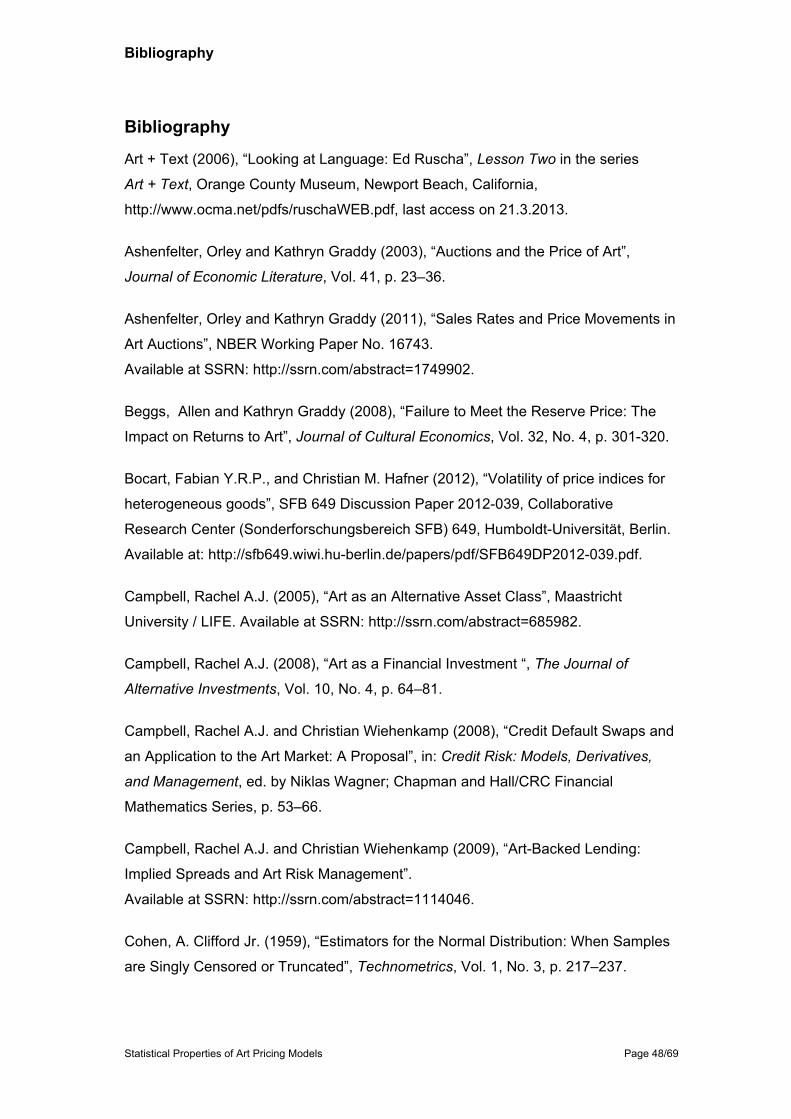
Bibliography


Bibliography

Art + Text (2006), “Looking at Language: Ed Ruscha”, Lesson Two in the series

Art + Text, Orange County Museum, Newport Beach, California,

http://www.ocma.net/pdfs/ruschaWEB.pdf, last access on 21.3.2013.

Ashenfelter, Orley and Kathryn Graddy (2003), “Auctions and the Price of Art”,

Journal of Economic Literature, Vol. 41, p. 23–36.

Ashenfelter, Orley and Kathryn Graddy (2011), “Sales Rates and Price Movements in

Art Auctions”, NBER Working Paper No. 16743.

Available at SSRN: http://ssrn.com/abstract=1749902.

Beggs, Allen and Kathryn Graddy (2008), “Failure to Meet the Reserve Price: The

Impact on Returns to Art”, Journal of Cultural Economics, Vol. 32, No. 4, p. 301-320.

Bocart, Fabian Y.R.P., and Christian M. Hafner (2012), “Volatility of price indices for

heterogeneous goods”, SFB 649 Discussion Paper 2012-039, Collaborative

Research Center (Sonderforschungsbereich SFB) 649, Humboldt-Universität, Berlin.

Available at: http://sfb649.wiwi.hu-berlin.de/papers/pdf/SFB649DP2012-039.pdf.

Campbell, Rachel A.J. (2005), “Art as an Alternative Asset Class”, Maastricht

University / LIFE. Available at SSRN: http://ssrn.com/abstract=685982.

Campbell, Rachel A.J. (2008), “Art as a Financial Investment “, The Journal of

Alternative Investments, Vol. 10, No. 4, p. 64–81.

Campbell, Rachel A.J. and Christian Wiehenkamp (2008), “Credit Default Swaps and

an Application to the Art Market: A Proposal”, in: Credit Risk: Models, Derivatives,

and Management, ed. by Niklas Wagner; Chapman and Hall/CRC Financial

Mathematics Series, p. 53–66.

Campbell, Rachel A.J. and Christian Wiehenkamp (2009), “Art-Backed Lending:

Implied Spreads and Art Risk Management”.


Cohen, A. Clifford Jr. (1959), “Estimators for the Normal Distribution: When Samples

are Singly Censored or Truncated”, Technometrics, Vol. 1, No. 3, p. 217–237.

Bibliography


Coleman, A.D. (1972), “I’m Not Really a Photographer”; in: The Last Picture Show:

Artists Using Photography, 1960–1982, exhibition catalogue, Walker Art Center

Minneapolis, Minnesota, 11.10.2003–4.1.2004, ed. by Douglas Fogle; Minneapolis,

2003, p. 22–23.

Csörgö, Sándor and Julian Faraway (1996), “The Exact and Asymptotic Distributions

of Cramér-von Mises Statistics”, Journal of the Royal Statistical Society. Series B

(Methodological), Vol. 58, No. 1, p. 221–234.

Deloitte (2011), “Emergence de l’Art comme nouvelle classe d’actifs”, Conférence

Nationale Suisse, 11 October 2011, Geneva.

Deng, Yongheng and John M. Quigley (2008), “Index Revision, House Price Risk,

and the Market for House Price Derivatives”.


Diebold, Francis X. (2004), “Elements of Forecasting”, Third Edition; Thomson

Southwestern, Mason, Ohio.

Edwards, Steve (2004), “Photography out of Conceptual Art”; in: Themes in

Contemporary Art, ed. by Gill Perry and Paul Wood; Yale University Press, New

Haven and London, p. 137–180.

Elton, Edwin J., Martin J. Gruber and Christopher R. Blake (1996), “Survivorship Bias

and Mutual Fund Performance”, The Review of Financial Studies, Vol. 9, No. 4,

p. 1097–1120.

Encz, Judith (2009), Ed Ruscha. Bild und Text. Konzepte gemalter Schriftzeichen,

Dissertation, Ludwig-Maximilian-University, Munich.

Gawrisch, Dimitrij (2008), “Price Determinants and Investment Characteristics of

Contemporary Paintings”, Master Thesis at the Institut für Finanzmanagement,

University of Berne.

Geltner, David Michael (1991), “Smoothing in appraisal-based returns”, The Journal

of Real Estate Finance and Economics, Vol. 4, Nr. 3, p. 327–345.

Ginsburgh, Victor, Jianping Mei and Michael Moses (2006), “On the Computation of

Price Indices”, in: Handbook of the Economics of Art and Culture, ed. by Victor A.

Ginsburgh and David Throsby; Elsevier, Amsterdam, p. 947–979.

Bibliography


Goetzmann, William N., Luc Renneboog and Christophe Spaenjers (2010a), “Art and

Money”, Version 14 January 2010; CentER Discussion Paper Series No. 2010-08.

Available at http://arno.uvt.nl/show.cgi?fid=99520, last access on 21.3.2013.

Goetzmann, William N., Luc Renneboog and Christophe Spaenjers (2010b), “Art and

Money”, Version 28 April 2010; Yale ICF Working Paper No. 09-26; TILEC

Discussion Paper No. 2010-002.

Available at SSRN: http://ssrn.com/abstract=1501171

Goetzmann, William N. and Matthew Spiegel (1995), “Private Value Components,

and the Winner’s Curse in an Art Index”, European Economic Review, Vol. 39, Issues

3/4, p. 549–555.

Hiraki, Takato, Akitoshi Ito, Darius Alexander Spieth, Naoya Takezawa (2005), “How

Did Japanese Investments Influence International Art Prices?”, Yale ICF Working

Paper No. 03-09; EFA 2005 Moscow Meetings Paper.


Iversen, Margaret (2010), „Auto-maticity: Ruscha and performative photography“; in:

Photography After Conceptual Art, ed. by Diarmuid Costello and Margaret Iversen;

Art History Special Issue Book Series, John Wiley & Sons Ltd., Chichester, West

Sussex (UK), p. 28–49.

Marzona, Daniel (2005), Conceptual Art, Taschen, Cologne.

McAndrew, Clare and Rex Thompson (2007), “The Collateral Value of Fine Art”,

Journal of Banking & Finance, 31, p. 589–607.

McAndrew, Clare, James L. Smith and Rex Thompson (2009), “The Impact of

Reservation Prices on the Perceived Bias of Expert Appraisals of Fine Art”.


McAndrew, Clare (2012), “The International Art Market in 2011: Observations on the

Art Trade over 25 Years”, ed. by Clare McAndrew; The European Fine Art

Foundation (TEFAF), Helvoirt.

Mei, Jianping and Michael Moses (2002), “Art as an Investment and the

Underperfomance of Masterpieces”, American Economic Review, Vol. 92, No. 5,

p. 1656–1668.

Bibliography


Okunev, John and Derek White (2003), “Hedge Fund Risk Factors and Value at Risk

of Credit Trading Strategies”. Available at SSRN: http://ssrn.com/abstract=460641.

Orlov, Michael L. (1996), “Multiple Linear Regression Analysis Using Microsoft

Excel”, Chemistry Department, Oregon State University,

http://chemistry.oregonstate.edu/courses/ch361-464/ch464/RegrssnFnl.pdf,

last access on 4.4.2013.

Ralevski, Olivia (2008), “Hedging the Art Market: Creating Art Derivatives”, Master

Thesis at the Management School, University of Edinburgh.

Renneboog, Luc and Christophe Spaenjers (2013), “Buying Beauty: On Prices and

Returns in the Art Market”, Management Science, Vol. 59, No. 1.

Rowell, Margit (2006), Ed Ruscha, Photographer, on the occasion of exhibitions in

Europe organised by the Whitney Museum of American Art, New York, ed. by Margit

Rowell; Steidl, Göttingen.

Salmon, Felix (2012), “Artnet’s silly indices”, http://blogs.reuters.com/felix-

salmon/2012/05/24/artnets-silly-indices/, last access on 8.3.2013.

Scorcu, Antonello Eugenio and Roberto Zanola (2011), “The ‘Right’ Price for Art

Collectibles: A Quantile Hedonic Regression Investigation of Picasso Paintings”, The

Journal of Alternative Investments, Vol. 14, No. 2, p. 89–99.

Skaterschikov, Sergey (2010), “Skate’s Art Investment Handbook”, Second Edition;

McGraw-Hill.

Stephens, Michael A. (1970), “Use of the Kolmogorov-Smirnov, Cramér-von Mises

and Related Statistics without Extensive Tables”, Journal of the Royal Statistical

Society. Series B (Methodological), Vol. 32, No. 1, p. 115–122.

Wiehenkamp, Christian (2007), “Art Credit Default Swap Pricing”, Master Thesis at

the Faculty of Economics and Business Administration, University of Maastricht.

Appendix


Appendix

Appendix A: Comparison of Ed Ruscha’s photographs to paintings and drawings at auctions

Photography is an essential medium for conceptual artists like Ed Ruscha in order to

realise their ideas. It is, however, unclear whether the photographs are fully

recognised in the art market, or whether they are traded with a discount compared to

drawings and paintings.

In order to find out the position of photographs compared to unique works we

study in this Appendix the prices paid for Ed Ruscha’s artwork at auctions. As

methodology, the hedonic regression analysis is used and different regressions are

performed with distinct features of the artworks as describing variables: Medium, size

of the artwork and the number of editions in the case of photographs. In addition, the

price development reflected by the index of Ed Ruscha’s artworks from Artprice

starting in 2000 is referred to, as well as the Art Market Research (AMR)

Contemporary Art Index as a proxy before the year 2000.

The results show that with the three variables, including size of the artwork, the

number of editions in the case of photographs and the index, the auction prices can

be explained to 65%. Further reducing the number of variables and neglecting the

photograph’s editions reduces the quality of the regression and gives an

unsatisfactory fit, especially for the photographs. Therefore, it can be concluded from

the regressions that the art market indeed distinguishes the photographs from

drawings and paintings insofar as it does take the editions of photographs into

account.

Data Selection

Ed Ruscha works in several media where photography is the most important one

beside paintings, and his photobooks were important contributions in the early days

of conceptual art.70 For the comparison with photographs, drawings and paintings are

taken into account. Ruscha’s photographs are closer in unique qualities to his

paintings and drawings than to his prints and multiples. The latter are therefore

neglected.

The data selection is based on the same original sample as described in Chapter

4.3.2. In total 731 entries were retrieved: 176 drawings, 473 paintings and 82

photographs. 19 entries were eliminated due to quality doubts:

70 See e.g. Coleman (1972). See also Chapter 4.3.1 for an introduction to Ed Ruscha.

Appendix


One entry due to a unrealistic low estimate,

18 sold works due to uncertainties whether the prices shown are hammer

prices (as indicated) or whether they include the buyer’s premium.

Disregarded here are works that have not been sold, i.e. the bought-ins, since the

price development is considered by an art index, which makes it necessary to have

an auction price. The bought-ins are in total 137 auction records. The bought-in rate

differs substantially per category: Whereas it is 16% and 19% for drawings and

paintings, respectively, the rate is 30% for photographs. This leads to a restricted

number of photographs thus reducing this already limited data sample even further.

Next to consider are only works where information on the size is available,

calculated as the area of the artwork, which eliminates 10 works. Dropped from

consideration are photographs without the number of editions indicated, which

reduces the sample by further 15 photographs. One photograph is excluded due to its

extraordinary large edition of 1200 prints and a corresponding low price of USD 500.

Since the considered price development index only started in 1988, five earlier

artworks are excluded.

Finally, there are 545 valid auction records which are shown per category in Table

6, together with the ratio of the final to the initial set.

Ed Ruscha’s auction results Total Drawings Paintings Photographs

Initial set 731 176 473 82 - Quality issues 19 5 14 0

- Bought-ins 137 27 85 25

- No information on size 10 0 5 5

- No information on edition 15 0 0 15

- Large edition 1 0 0 1

- Auctioned before 1988 5 2 3 0

Final set 545 143 366 36 Ratio of final to initial set 75% 84% 77% 44% Table 6 Ed Ruscha’s auction results for drawings, paintings and photographs until 30.11.2012. The second column contains the sum of the figures in the columns three to five. The second row shows the initial data set that has been retrieved from Artprice on 26 and 27 December 2012. The rows three to eight contain the numbers of excluded records due to quality issues, missing prices (i.e. bought-ins), missing information on size and (photo) edition, too large edition size and auctions before 1988, respectively. The ninth row (bold) represents the final data set that is used in the analysis, and the last row shows the ratio of the final to the initial set. Data is taken from: www.artprice.com, last access on 27.12.2012.

Appendix


Figure 18 shows the distribution of the auction prices of the final set per category

compared to the prices (x-axis). The prices are mapped according to a logarithm with

base 2, i.e. )(log2 Price , in order to better visualise the lower priced artworks, which

dominate the sample. It is obvious that the paintings (dark blue bars; bottom layer)

cover the higher price region, whereas the drawings (light green bars; middle layer)

are most prominent between USD 20’000 and USD 200’000, and the photographs

(orange bar; top layer) are limited to below USD 200’000.71

Auction price distribution of Ed Ruscha's sales

0

20

40

60

80

100

3 6 13 25 50 100 200 400 800 1'600 3'200 6'400 12'800

Price in Thousand USD (logarithmic scale)

Dis

tribu

tion Photographs

Drawings

Paintings

Figure 18 Distribution of auction prices for artworks of Ed Ruscha. The prices (x-axis) are scaled according to a logarithm with base 2, i.e. )(log2 Price . The paintings are the dark blue bars (bottom layer), the drawings are the light green bars (middle layer) and the photographs are the orange bars (top layer). The chart shows the final set in Table 6 (545 data points). Data is taken from: www.artprice.com, last access on 27.12.2012.

Hedonic Regression

As described in Chapter 2, hedonic regression is a technique used to find relations

between features of a good and a variable to be explained. Typically this variable is

the (transaction) price, and the attributes of the good are taken as measureable and

fixed input in order to establish a predictable relation.

The goal of this Appendix is to explain the prices at auction of Ed Ruscha by

means of a few features of drawings, paintings and photographs. The choice of the

variables is:

Medium: Paintings are worth more than drawings, and both are expected to

be higher priced than photographs.

Size: Intuitively one expects a higher price for a larger artwork.

71 The reader should keep in mind that the prices are nominal prices not adjusted for inflation or for a price development of the work between the date when the auction took place and today.

Appendix


Number of editions in the case of photographs: The larger the edition the

lower the price for a single print.

Index: Market development of Ed Ruscha’s artworks to adjust for the

historical prices in order to get the present value of the auctioned works.

The low number of variables should allow for a straightforward explanation of the

results. Increasing the number of variables most likely gives a higher degree of

numerical precision. However, the interpretation gets harder when more variables are

considered.72

The mathematical expression for the hedonic regression of the price of an artwork

reads73

)ln()ln(

)ln()ln(

54

3210

Indexedition Photo

SizePrice PaintingDrawing 11 (A.1)

where )ln(X is the natural logarithmic function and Y1 is the indicator function for

drawings and paintings, respectively. E.g.

otherwise0

drawing medium casein 1Drawing1 .

Size is the area of the artwork, i.e. height times width, edition Photo is the number of

prints in the case of photographs, and Index reflects the price development of Ed

Ruscha’s artwork explained below. i are the parameters to be determined, valid for

all the art works in the data set, and is a residual term, which contains the

unexplained part of the price.

After applying the exponential function )exp(x to both sides of eq.(A.1) we obtain

the following equation for the price relation,

543 edition Photoexp 210 IndexSizePrice PaintingDrawing 11 (A.2)

The influence of the parameters i on the price can be read off from eq.(A.2).

The price development is represented by the index of Ed Ruscha’s artworks from

Artprice starting in 2000. For the pre-2000 time period we use as a proxy the Art

Market Research (AMR) Contemporary Art Index starting in 1987.74 Since the index

is built from price averages, which lead to a smoothed time-series, we use a de-

smoothed version of the index, which has a substantially higher volatility than the

reported time-series.75 Ruscha’s Artprice index is regressed to the de-smoothed AMR

72 Potential extensions include the subject of a work or the technique used in paintings. 73 Ginsburgh et al (2006). 74 See Chapter 3.3. 75 Ibid.

Appendix


Contemporary Art Index for the period in which both exist in parallel, from 2000 to

2010. The resulting excess return and the market factor Market are assumed to be

valid also before year 2000,

Artry ContemporaMarketRuscha Ed IndexIndex ,

with the idiosyncratic error term . At the 1%-confidence level the parameters are

0 and 700.0Market (with an adjusted 41.02 R ).

The goodness-of-fit, expressed in 2R , is not very high, essentially due to 2008: In

that year the Contemporary Art Index still increased, while the prices for Ruscha’s

artwork already started decreasing.

The final index used in the analysis is constructed in the following way

later and 2000year

2000year before7.0

Ed Ruscha

ry Art Contempora

IndexIndex

Index .

Results

The information on the final data sample is put into eq.(A.1) and the linear regression

is solved. The goal is to find the parameter set i that gives the best description of

the auction prices. The procedure used is called Ordinary Least Squares (OLS),

which measures the difference, called error, between each individual auction price

and the corresponding theoretical price from the model, squares these differences

and sums them up. The optimal solution is determined by the set of parameters i

that minimises the sum of the squared errors. Once a solution is found a check is

performed on the relevance of the describing variables and as many irrelevant ones

as possible are eliminated. An optimisation for the parameters i has to be

conducted on each restricted set of parameters.

For the goodness-of-fit we refer to the adjusted 2R , which is between zero and

one, and the higher the value the better the precision. 12 R means perfect

coincidence. For the rejection of variables we use the p -value, which indicates at

which level the variable is significant, i.e. should not be rejected. The lower the better:

Significance is usually associated with a p -value below 5%. As a tool for solving the

linear regression we use Microsoft Excel.76

The first regression is done with all the parameters i and shown in Table 7. For

the intercept and for the distinction between the media drawings and paintings it can

76 For a tutorial explanation of the regression tool in Microsoft Excel and of the quantities mentioned in this Chapter we refer to Orlov (1996).

Appendix


be seen that the coefficients are not significantly different from zero since the

standard errors are larger than the coefficients themselves. This is confirmed by the

probability to reject these coefficients. On the other hand the size, the amount of

editions for photographs and the price development are highly significant, all at or

below the 1%-level and with very small errors, except the photo edition variable. The

quality of the fit is good, %0.652 R , i.e. on average almost two thirds of an auction

price can be explained by the chosen parameters.

Variable Parameter Coefficient Standard error Significance

Intercept 0 0.803 1.237 51.6%

Drawing 1 -1.050 1.150 36.1%

Painting 2 -0.971 1.148 39.8%

Size 3 0.582 0.036 < 1%

Photo edition 4 -0.848 0.335 1.2%

Index 5 1.167 0.050 < 1%

2R 0.650

Table 7 Result from the first regression with all parameters in eq.(A.1). For each explaining variable we indicate the coefficient, the standard error and the level of significance. The last row contains the quality of the fit.

Next, the first three parameters 0 to 2 are set to zero and the regression is

repeated with the remaining parameters. The result is shown in Table 8. While the

coefficients for the size and the index remained almost unchanged with even smaller

errors than in the first regression, the relevance of the photograph’s editions

increased substantially now having an error comparable to the other two variables.

Since the quality of the fit, %2.652 R , remained almost unchanged compared to

the first regression, the second regression with less parameters is superior to the first

regression. All variables are highly significant. The resulting logarithmic prices of this

regression are shown in Figure 19 compared to the corresponding auction prices.

The paintings are on the upper end of the scale, and the photographs at the lower

end.

As a third and last regression the question is whether the number of editions for

photographs really matters. Are the photographs treated differently from paintings

and drawings? In this case we set 04 , and repeat the regression with the two

remaining variables.

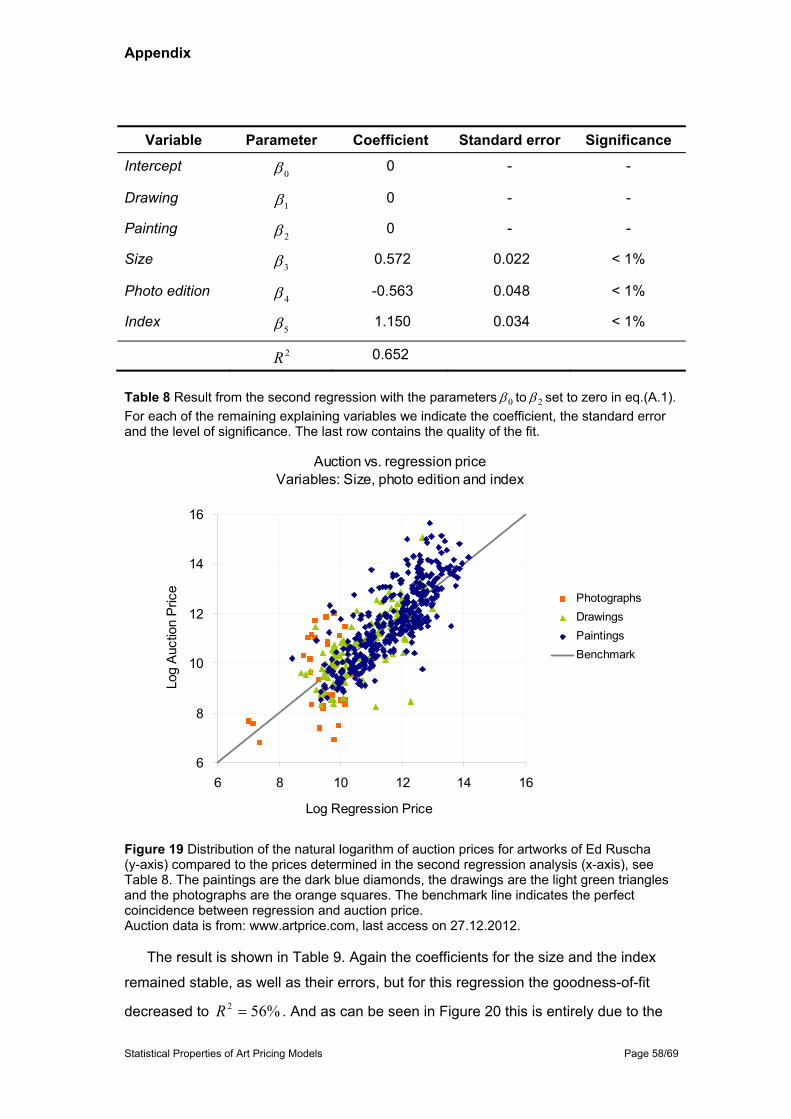
Appendix



Intercept 0 0 - -

Drawing 1 0 - -

Painting 2 0 - -

Size 3 0.572 0.022 < 1%

Photo edition 4 -0.563 0.048 < 1%

Index 5 1.150 0.034 < 1%

2R 0.652

Table 8 Result from the second regression with the parameters 0 to 2 set to zero in eq.(A.1). For each of the remaining explaining variables we indicate the coefficient, the standard error and the level of significance. The last row contains the quality of the fit.

Auction vs. regression price Variables: Size, photo edition and index

6

8

10

12

14

16

6 8 10 12 14 16

Log Regression Price

Log

Auct

ion

Pric

e

PhotographsDrawingsPaintingsBenchmark

Figure 19 Distribution of the natural logarithm of auction prices for artworks of Ed Ruscha (y-axis) compared to the prices determined in the second regression analysis (x-axis), see Table 8. The paintings are the dark blue diamonds, the drawings are the light green triangles and the photographs are the orange squares. The benchmark line indicates the perfect coincidence between regression and auction price. Auction data is from: www.artprice.com, last access on 27.12.2012.

The result is shown in Table 9. Again the coefficients for the size and the index

remained stable, as well as their errors, but for this regression the goodness-of-fit

decreased to %562 R . And as can be seen in Figure 20 this is entirely due to the

Appendix


worse fit for the photographs which strongly deviate from the indicated benchmark as

perfect coincidence between the observed auction prices and the calculated prices

from the regression. Therefore the third regression is considered less reliable than

the second regression.


Intercept 0 0 - -

Drawing 1 0 - -

Painting 2 0 - -

Size 3 0.566 0.021 < 1%

Photo edition 4 0 - -

Index 5 1.159 0.032 < 1%

2R 0.563

Table 9 Result from the third regression with the parameters 0 to 2 and 4 set to zero in eq.(A.1). For each of the remaining explaining variables we indicate the coefficient, the standard error and the level of significance. The last row contains the quality of the fit.

Auction vs. regression price Variables: Size and index

6

8

10

12

14

16

6 8 10 12 14 16

Log Regression Price

Log

Auct

ion

Pric

e

PhotographsDrawingsPaintingsBenchmark

Figure 20 Distribution of the natural logarithm of auction prices for artworks of Ed Ruscha (y-axis) compared to the prices determined in the third regression analysis (x-axis), see Table 9. The paintings are the dark blue diamonds, the drawings are the light green triangles and the photographs are the orange squares. The benchmark line indicates the perfect coincidence between regression and auction price. Auction data is from: www.artprice.com, last access on 27.12.2012.

Appendix


Interpretation

Consequently, the interpretation of the results is done on the second regression as

listed in Table 8. The coefficients indicate that the size and the index have both a

positive impact on the price, while the number of editions of photographs influences

the price downwards. The coefficient for the index is very close to one, which comes

as no surprise since it is assumed that the index, at least after the year 2000, reflects

the price movement of Ed Ruscha’s artworks. Also the other two coefficients are

explainable by intuition: The larger the size of the artwork, the higher the price, and

the larger the photograph’s edition, the lower the price.

The results are transformed into eq.(A.2) for the numerical interpretation,77

15.156.057.0 Indexedition PhotoSizePrice .

In a rough approximation, the price formula can be reduced to square roots of the

size and the edition and a slightly increased dependence on the index,78

45

Indexedition Photo

SizePrice .

which means that the price increases with the square root of the area, and

decreases with the square root of the number of photograph editions. The former

finding is in line with the practice to sum height and width of an artwork in order to

determine the price of a work, rather to scale it with the area. The latter tells us that

although the market is aware of the number of prints it does not linearly account for it.

For example: If an edition is four times as numerous as another one, the price for a

single print out of this “big” edition is expected to be half the price as for a photograph

out of the edition with fewer prints.

An extension of this study could include the subject of a work as a regression

parameter. Or to include a more detailed differentiation for the largest category, the

paintings, by e.g. including the paints (oil, acrylic, etc.) as explaining variables in

order to further improve the goodness-of-fit. A further possibility is the determination

of the regression parameters per medium, and to check whether they are medium-

dependent.

77 The residual term is dismissed for this discussion. 78 If the coefficients of the size and the edition are set to 5.03 and 5.04 , the

regression results in 01.025.15 for the index coefficient.

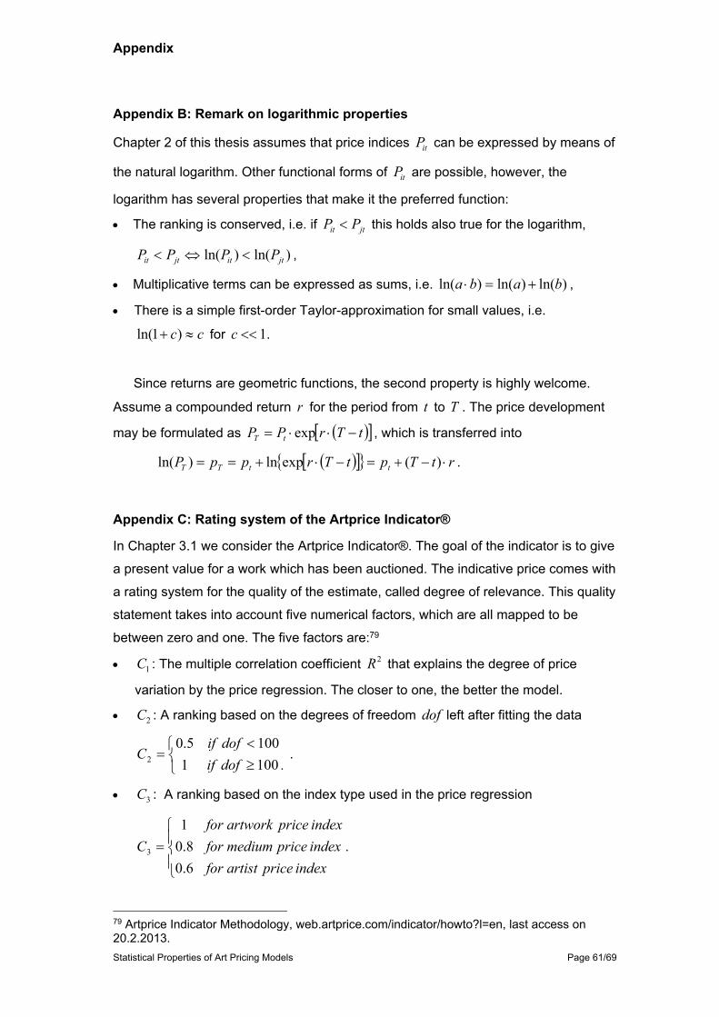
Appendix


Appendix B: Remark on logarithmic properties

Chapter 2 of this thesis assumes that price indices itP can be expressed by means of

the natural logarithm. Other functional forms of itP are possible, however, the

logarithm has several properties that make it the preferred function:

The ranking is conserved, i.e. if jtit PP this holds also true for the logarithm,

)ln()ln( jtitjtit PPPP ,

Multiplicative terms can be expressed as sums, i.e. )ln()ln()ln( baba ,

There is a simple first-order Taylor-approximation for small values, i.e.

cc )1ln( for .1c

Since returns are geometric functions, the second property is highly welcome.

Assume a compounded return r for the period from t to T . The price development

may be formulated as tTrPP tT exp , which is transferred into

rtTptTrppP ttTT )(expln)ln( .

Appendix C: Rating system of the Artprice Indicator® In Chapter 3.1 we consider the Artprice Indicator®. The goal of the indicator is to give

a present value for a work which has been auctioned. The indicative price comes with

a rating system for the quality of the estimate, called degree of relevance. This quality

statement takes into account five numerical factors, which are all mapped to be

between zero and one. The five factors are:79

1C : The multiple correlation coefficient 2R that explains the degree of price

variation by the price regression. The closer to one, the better the model.

2C : A ranking based on the degrees of freedom dof left after fitting the data

. dof if dof if

C10011005.0

2 .

3C : A ranking based on the index type used in the price regression

index price artist forindex price medium forindex price artwork for

C

6.08.0

1

3 .

79 Artprice Indicator Methodology, web.artprice.com/indicator/howto?l=en, last access on 20.2.2013.

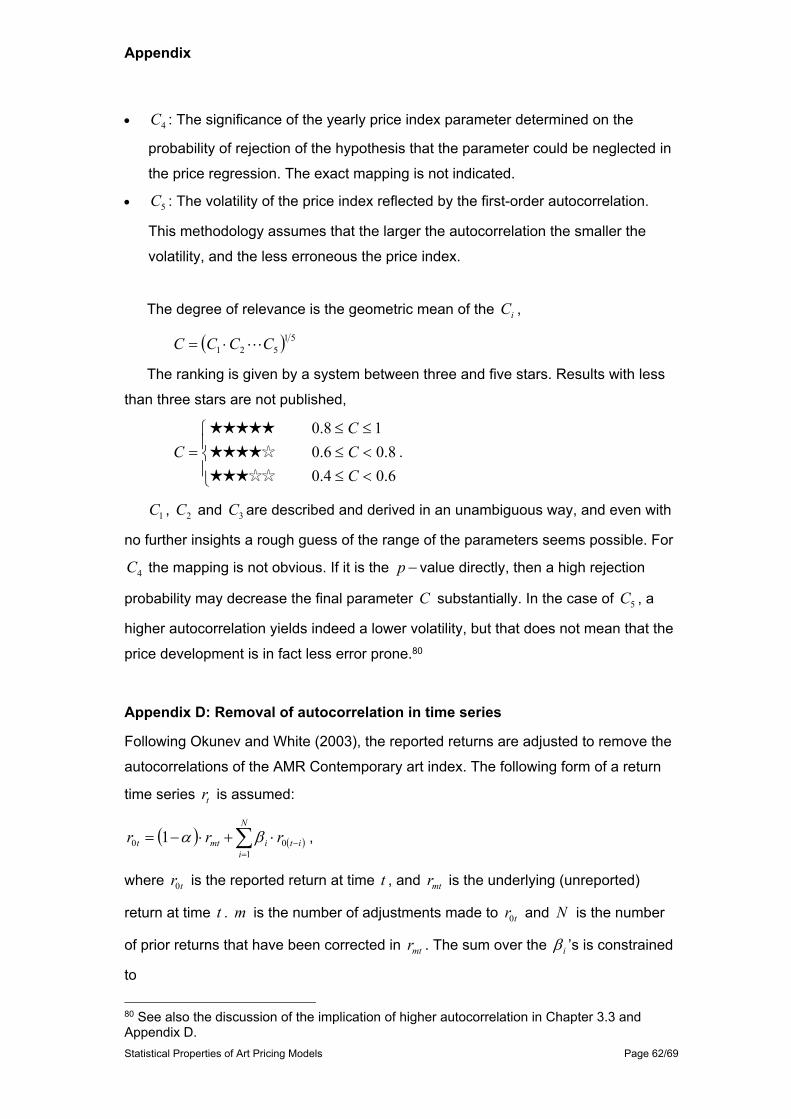
Appendix


4C : The significance of the yearly price index parameter determined on the

probability of rejection of the hypothesis that the parameter could be neglected in

the price regression. The exact mapping is not indicated.

5C : The volatility of the price index reflected by the first-order autocorrelation.

This methodology assumes that the larger the autocorrelation the smaller the

volatility, and the less erroneous the price index.

The degree of relevance is the geometric mean of the iC ,

51521 CCCC

The ranking is given by a system between three and five stars. Results with less

than three stars are not published,

6.04.08.06.0

18.0

CCC

C

.

1C , 2C and 3C are described and derived in an unambiguous way, and even with

no further insights a rough guess of the range of the parameters seems possible. For

4C the mapping is not obvious. If it is the p value directly, then a high rejection

probability may decrease the final parameter C substantially. In the case of 5C , a

higher autocorrelation yields indeed a lower volatility, but that does not mean that the

price development is in fact less error prone.80

Appendix D: Removal of autocorrelation in time series Following Okunev and White (2003), the reported returns are adjusted to remove the

autocorrelations of the AMR Contemporary art index. The following form of a return

time series tr is assumed:

N

iitimtt rrr

100 1 ,

where tr0 is the reported return at time t , and mtr is the underlying (unreported)

return at time t . m is the number of adjustments made to tr0 and N is the number

of prior returns that have been corrected in mtr . The sum over the i ’s is constrained

to

80 See also the discussion of the implication of higher autocorrelation in Chapter 3.3 and Appendix D.

Appendix


N

ii

1 .81

The methodology of the elimination of the first order autocorrelation can be traced

back to Geltner (1991) who used the procedure in order to de-smooth real estate

returns. The relation to get the first corrected return series tr1 reads:

1

10101 1 c

rcrr tt

t

,

where 1c is the coefficient to be determined. The derivation of the general solution for

1c can be found in Okunev and White (2003). In order to remove the first order

autocorrelation completely, 1c becomes

01

201

20202

1 2411

aaaa

c

, (D.1)

where 01a and 02a are the first and second order autocorrelations of the reported

return series tr0 , respectively,

21],, 000 ,q aaCorr[a qttq .

For later use mqa is defined as the qth order autocorrelation of the m times

corrected return series mtr ,

],Corr[ qtmmtmq aaa .

Eq.(D.1) only has a real solution if 202201 14 aa . Assuming for a moment that the

higher autocorrelations are negligible, tr0 can be written as

101110 1 ttt rcrcr ,

and the corresponding variance is

][Var

121][Var ][Var][Var1 02

1

01121

1101012

1 ttttt rc

accrrcrrc

.

Since 11 01 a we have for :01 c

2101121 121 cacc ,

81 Note that in Okunev and White (2003) the sum over the i ’s is erroneously given to be

equal to 1 .

Appendix


and ][Var][Var 01 tt rr , i.e. the variance of the corrected return series is larger than

the reported return series in case 1c is positive. Therefore, having a positive first

order autocorrelation underestimates the volatility in the smoothed (reported) returns.

We can repeat the removal of the autocorrelation to the second order, now

working on the corrected series tr1 . The two times corrected return series tr2

becomes analogously,

2

21212 1 c

rcrr tt

t

and 2c is

12

212

21414

2 2411

aaaa

c

with a real solution if 214212 14 aa . An approximate form of the de-smoothed

returns can be derived by neglecting cross-terms of second order,

212021012210 1 ccOrcrcrccr tttt .

Again, the variance ][Var 2tr is larger than ][Var 1tr in case 2c is positive.

Due to the removal of the second order autocorrelation and the corresponding

change in the time series, it cannot be avoided that again a first order autocorrelation

is introduced into the return series tr2 . Okunev and White (2003) describe in detail

the iterative procedure to remove again the first order autocorrelation in the same

manner as shown above. Numerically, however, the effects are rather small. In

AMR’s Contemporary art index the autocorrelations are removed straightforwardly

finding that the newly induced autocorrelations can be left uncorrected since the new

autocorrelation coefficients are below the 95% confidence level for a normal

distribution with zero mean and a standard deviation of T1

, where 305T is the

total number months considered.82 The critical band at 95% confidence level lies

therefore within 112.030596.1 .

In a generalised form we can write the returns mtr and the corresponding

coefficient mqc , which eliminates the qth order autocorrelation in the m times

corrected return series mtr ,

82 See Diebold (2004), p. 137–140.

Appendix


mq

qtmmqtmmt c

rcrr

111

and

qm

qmqmqmmq a

aaac

1

21

22121

2411

with a real solution if 2212

1 14 qmqm aa . For each 0mqc the variance

increases and for each 0mqc the variance decreases.

Appendix E.1: Expected loss for art backed loans

In Campbell and Wiehenkamp (2009), the expected loss EL for the bank due to the

loan is written as

dtttqELT

O

,

where tq is the time-dependent default probability function for the specific

borrower, and t is the loss function,

otherwise

t time at default of case ini PP

trPt tLoan

Artt

tfLoan

0

1,min~1exp0

0

LoanP0 is the loan valued at time 0t , trf exp is the discount factor for the

present value of the loan, and ti is the accrued interest. t~ reflects the availability of

buyers in case of an urgent liquidation of the artwork, and Arttp is the assumed price

of the underlying artwork at time t .

Campbell and Wiehenkamp (2009) consider data from Sotheby’s London with

mostly Impressionist paintings, Victorian pictures, Old Masters, 16th century British

paintings and Modern Art. The final data set contains 398 repeat-sales pair and its

empirical return distribution is fitted to the normal, logistic and t -Student distributions.

The authors find that out of the three statistical functions the t -Student distribution

gives the closest description of the data. This specific data fitted t -Student

distribution is used to simulate the loss function )(t .83

83 The buyer availability function t

~ is assumed to be a Poisson distribution, see Campbell and Wiehenkamp (2009).

Appendix


Appendix E.2: Artworks as collateral values in bank loans

The approach of McAndrew and Thompson (2007) considers the loss given default in

case the borrower is unable to pay back the bank loan (or pay the interest). The

authors assume that the valuation of the artwork can be done based on the auction

history of a single artist, the period for different artists or other criteria leading to

comparable art objects. The method is time-invariant, i.e. it assumes that the

observed prices in relation to the pre-sale estimates are unconditional to the point in

time. The loss given default LGD is defined as

LTV

LTV dxxgxdxxgLTV

LGD0

0

)()(

11 ,

where LTV is the loan-to-value ratio and )(xg is the distribution function of the

auction prices.

Appendix F: Statistical tests

Three tests are performed for the cumulative distribution function in Chapter 4.2 in

order to test the null-hypothesis ii xYxFH )(:0 , i.e. that the assumed t -Student

distribution ixF is the correct distribution to describe the empiric cumulative

distribution function ixY . ixY is determined from the observations ix , which are

indexed in ascending order, nxxx 21 , and can therefore be written as

ninixY i ,2,1 , .

Kolmogorov-Smirnov test

In the Kolmogorov-Smirnov test the maximum maxd is determined from the point wise

distances between ixF and ixY , and its next neighbour 1ixY , i.e.

nn bbaad ,...,;,,max 11max

with

nixFa ii )( , and

n

ixFb ii1)(

.

For 40n a critical distance critd is given by a simple formula dependent on the

confidence level ,

Appendix


2ln

21

ndcrit .

If )(max critdd then the null-hypothesis 0H that )( ixF is the correct distribution

for the empirical cumulative distribution function ixY , ii xYxFH )(:0 has to be

rejected at the confidence level .

Cramér-von Mises and Anderson-Darling tests

Other tests measure the weighted piecewise difference of the area between )(xF

and ixY . A convenient way to write the sum of squared differences is

1

0

22 )()()()( xdFxxYxFnQn ,

where the weight function )(x will be determined below, and )(xY is a step function

for the purpose of the integral representation; a transformation of the integral to a

sum is then performed for the aim of the calculation.

For the Cramér-von Mises test the weight is 1)( xCvM , and the test measures

mainly the deviation around the mean of )(xF . The integral can be expressed as a

sum,84

2

1

1

0

22

212

121)()()(

n

iin xF

ni

nxdFxYxFnW .

The critical values for 2nW are tabulated for specific number of observations and

confidence levels .85

The Anderson-Darling test, finally, is similar to the Cramér-von Mises test;

however, it introduces a different weight in the integral,

)(1)(1)(

xFxFxAD ,

which gives more weight to the tails and leads to the squared standardised difference

between the empirical cumulative distribution )(xY and the assumed cumulative

distribution function )(xF .

84 See e.g. http://www.aiaccess.net/English/Glossaries/GlosMod/e_gm_goodness_of_fit.htm, last access on 20.1.2013. 85 See Stephens (1970); Csörgö and Faraway (1996).

Appendix


Again, the integral can be expressed as a sum,86

ini

n

i

n

xFxFin

n

xdFxFxF

xYxFnA

11

1

0

22

1lnln)12(1

)()(1)(

)()(

2nA gives a p -value with which the null-hypothesis ixYxFH )(:0 can be

directly tested.

Appendix G: Estimate of mean and standard deviation for a truncated normal distribution

The approach by Cohen (1959) considers a normal distribution that is truncated or

censored in one of the tails and yields the mean and standard deviation of the

complete distribution by means of a functional form. The needed input consists of the

sample data above or below the threshold where the distribution is truncated, and of

the number of the dismissed data points. It links the mean x and the variance 2s of

the upper or lower tail to the mean and the variance 2 of the full distribution,

under the assumption that it is normal distributed. The connection reads

,,

,,1

,~,

,~,

2

2

2

222

txs

nnn

txns

txnx

l

ll

l

l

(G.1)

and

,

,1

,

,,

,,

NNn

nnn

nnn

ll

N

N

l

ll

l

ll

where btt ln~ is the truncation point for the normal distribution function, lN is the

number of truncated data points and N is the complete number of the empirical data

86 cf. note 84.

Appendix


points.87 N and N are the standard normal density and cumulative function,

respectively, evaluated at . Solving the third equation of eq.(G.1) for , and

therefore ,ln , we find ,ln and can consequently solve the first two

equations for and 2 , which then are the location and scale parameters for the

lognormal distribution, respectively. In this study we consider the upper tail and have

279.0x , 123.02 s , 154.0~ t , 299lN and 690N .

87 Note that in McAndrew and Thompson (2007), p. 598, lN is incorrectly associated with the

number of data points above the threshold t~ .

statistical properties of - uzh

Documents