Statistical Properties of Wave Chaotic Scattering and Impedance Matrices

MURI Faculty: Tom Antonsen, Ed Ott, Steve Anlage,

MURI Students: Xing Zheng, Sameer Hemmady, James Hart

AFOSR-MURI Program Review

Electromagnetic Coupling in Computer Circuits

connectors

cables

circuit boards

Integrated circuits

Schematic• Coupling of external radiation to computer circuits is a complex processes:

aperturesresonant cavitiestransmission linescircuit elements

• Intermediate frequency range involves many interacting resonances

• System size >> Wavelength

• Chaotic Ray Trajectories

• What can be said about coupling without solving in detail the complicated EM problem ?

• Statistical Description !(Statistical Electromagnetics, Holland and St. John)

Z and S-MatricesWhat is Sij ?

V1

V2

VN1

S

V1

V2

VN1

outgoing incoming

S matrix

S (Z Z0 ) 1(Z Z0)

• Complicated function of frequency• Details depend sensitively on unknown parameters

Z() , S()

N- PortSystem

•••

V1

V1

VN

VN

N ports • voltages and currents, • incoming and outgoing waves

V1, I1

VN, IN

V1

V2

VN

Z

I1

I2

I2

voltage current

Z matrix

Random Coupling Model

0

0.2

0.4

0.6

0.8

1

1.2

0 0.5 1 1.5 2 2.5

integrablechaotic A

s

chaotic B

3. Eigenvalues kn2 are distributed according

to appropriate statistics:

- Eigenvalues of Gaussian Random Matrix

sn (kn12 kn

2) / k2Normalized Spacing

2. Replace exact eigenfunction with superpositions of random plane waves

n limN Re2

ANak exp i knek x k

k1

N

Random amplitude Random direction Random phase

1. Formally expand fields in modes of closed cavity: eigenvalues kn = n/c

Statistical Model of Z MatrixFrequency Domain

Port 1

Port 2

Other ports

Losses

Port 1

Free-space radiationResistance RR()ZR() = RR()+jXR ()

RR1()

RR2()

Zij ()j

RRi1/2(n )RRj

1/2(n)n

2 winw jn

2(1 jQ 1) n2

n

Statistical Model Impedance

Q -quality factor

n - mean spectral spacing

Radiation Resistance RRi()

win- Gaussian Random variables

n - random spectrum

Systemparameters

Statisticalparameters

Model ValidationSummary

Single Port Case:

Cavity Impedance: Zcav = RR z + jXR

Radiation Impedance: ZR = RR + jXR

Universal normalized random impedance: z + j

Statistics of z depend only on damping parameter: k2/(Qk2)(Q-width/frequency spacing)

Validation:HFSS simulationsExperiment (Hemmady and Anlage)

Normalized Cavity Impedance with Losses

Port 1 Losses

Zcav = jXR+(+j RR

Theory predictions forPdf’s of z=+j

Distribution of reactance fluctuationsP()

k2

Distribution of resistance fluctuationsP()

k2

Two Dimensional Resonators

• Anlage Experiments• HFSS Simulations• Power plane of microcircuit

Only transverse magnetic (TM) propagate forf < c/2h

Ez

HyHx

h

Box withmetallic walls

ports

Ez (x, y)VT (x, y) / h

Voltage on top plate

HFSS - SolutionsBow-Tie Cavity

Moveable conductingdisk - .6 cm diameter“Proverbial soda can”

Curved walls guarantee all ray trajectories are chaoticLosses on top and bottom plates

Cavity impedance calculated for 100 locations of disk4000 frequencies6.75 GHz to 8.75 GHz

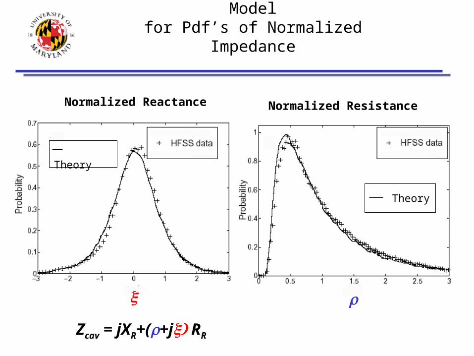
Comparison of HFSS Results and Modelfor Pdf’s of Normalized Impedance

Normalized Reactance Normalized Resistance

Zcav = jXR+(+j RR

Theory

Theory

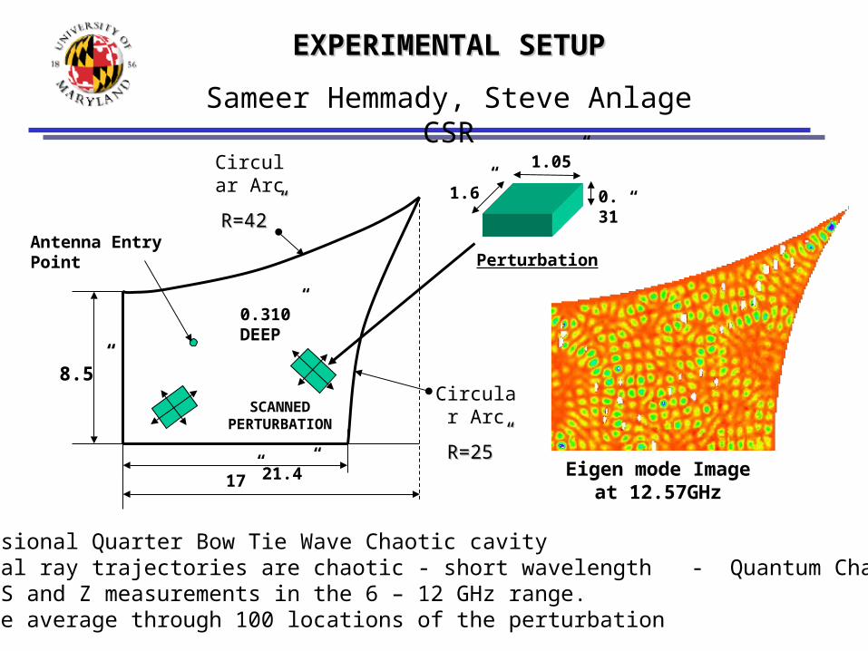
EXPERIMENTAL SETUPEXPERIMENTAL SETUP

Sameer Hemmady, Steve Anlage CSR

Eigen mode Image at 12.57GHz

8.5”

17” 21.4”

0.310” DEEP

Antenna Entry Point

SCANNED PERTURBATION

Circular Arc

R=25”R=25”

Circular Arc

R=42”R=42”

2 Dimensional Quarter Bow Tie Wave Chaotic cavity Classical ray trajectories are chaotic - short wavelength - Quantum Chaos 1-port S and Z measurements in the 6 – 12 GHz range. Ensemble average through 100 locations of the perturbation

0. 31”

1.05”

1.6”

Perturbation

0 1 2 30

1

2

k2 / (k 2Q) 7.6

k2 / (k 2Q) 4.2

k2 / (k 2Q) 0.8

-2 -1 0 1 20

1

2

k2 / (k 2Q) 0.8

k2 / (k 2Q) 4.2

k2 / (k 2Q) 7.6

Re Z / RR

(Im Z XR) / RR

High LossLow Loss Intermediate Loss

Comparison of Experimental Results and Modelfor Pdf’s of Normalized Impedance

Theory

Normalized Scattering AmplitudeTheory and HFSS Simulation

Theory predicts:

P( s ,)1

2Ps ( s )

Uniform distribution in phase

Actual Cavity Impedance: Zcav = RR z + jXR

Normalized impedance : z + jUniversal normalized scattering coefficient: s = (z)/(z) = | s| exp[ i]Statistics of s depend only on damping parameter: k2/(Qk2)

Experimental Distribution of Normalized Scattering Coefficient

0 20 40 60 80 1000

20

40

60

80

100

a))Im(s

1

-1

0

1-1

0 )Re(s

s=|s|exp[i]

Theory

|s|2

ln [P(|s|2)]Distribution of Reflection Coefficient

Distribution independent of

Frequency Correlations in Normalized ImpedanceTheory and HFSS Simulations

Zcav = jXR+(+j RR

RR = <((f1)-1)((f2)-1)>

XX = <(f1)(f2)>

RX = <((f1)-1 )(f2)>

(f1-f2)

Properties of Lossless Two-Port Impedance(Monte Carlo Simulation of Theory Model)

Eigenvalues of Z matrix

det Z jX 1 0

X1,2X

R

1, 2R

R

1,2 tan1,2

2

Individually 1,2 are Lorenzian distributed

1

2

Distributions same asIn Random Matrix theory

HFSS Solution for Lossless 2-Port

2

1

Joint Pdf for 1 and 2

Port #1:

Port #2:

Disc

Comparison of Distributed Lossand Lossless Cavity with Ports

(Monte Carlo Simulation)

Distribution of reactance fluctuationsP()

Distribution of resistance fluctuationsP()

Zcav = jXR+(+j RR

d2

dt2 2nddt

n2

Vn(t)

1

RR(n)n2wn

2

n

ddt

I(t)

Time Domain

V( t) Vn (t)n

n n

Q

wn- Gaussian Random variables

Time Domain Model for Impedance Matrix

Z() j

RR (n)n

n2 wn

2

2(1 jQ 1) n2

n

Frequency Domain

Statistical Parameters

wn- Gaussian Random variables

n - random spectrum

Incident and Reflected Pulsesfor One Realization

-1

-0.5

0

0.5

1

0 0.02 0.04 0.06 0.08 0.1 0.12

Inci

dent

Vol

tage

t [sec]

Incident Pulse

-1

-0.5

0

0.5

1

0 0.02 0.04 0.06 0.08 0.1 0.12

Ref

lect

ed V

olta

ge

t [sec]

Prompt Reflection

Delayed Reflection

Prompt reflection removed by matching Z0 to ZR

f = 3.6 GHz = 6 nsec

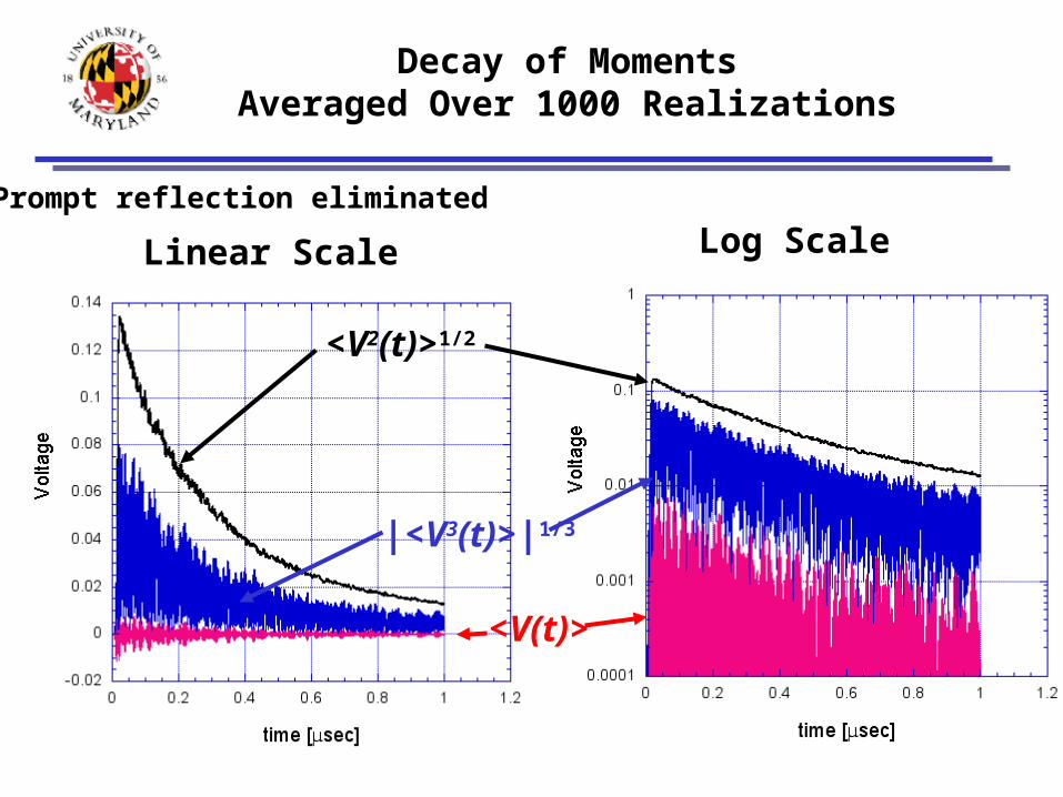
Decay of MomentsAveraged Over 1000 Realizations

<V(t)>

<V2(t)>1/2

|<V3(t)>|1/3

Linear Scale Log ScalePrompt reflection eliminated

Quasi-Stationary Process

-1

-0.5

0

0.5

1

1.5

2

2.5

-1.5 10-8 -1 10-8 -5 10-9 0 5 10-9 1 10-8 1.5 10-8

<u(

t 1)u

(t2)>

t1-t

2

t1 = 1.0 10-7

t1 = 8.0 10-7

t1 = 5.0 10-7

Normalized Voltageu(t)=V(t) /<V2(t)>1/2

2-time Correlation Function(Matches initial pulse shape)

-1

-0.5

0

0.5

1

0 0.02 0.04 0.06 0.08 0.1 0.12

Inci

dent

Vol

tage

t [sec]

Incident Pulse

Histogram of Maximum Voltage

0

20

40

60

80

100

120

0 0.05 0.1 0.15 0.2 0.25 0.3 0.35 0.4 0.45 0.5 0.55

Cou

nt

|V(t) |max

1000 realizations

Mean = .3163

|Vinc(t)|max = 1V

Progress

• Direct comparison of random coupling model with -random matrix theory -HFSS solutions -Experiment

• Exploration of increasing number of coupling ports

• Study losses in HFSS • Time Domain analysis of Pulsed Signals

-Pulse duration-Shape (chirp?)

• Generalize to systems consisting of circuits and fields

Current

Future

Role of Scars?

• Eigenfunctions that do not satisfy random plane wave assumption

Bow-Tie with diamond scar

• Scars are not treated by either random matrixor chaotic eigenfunction theory

• Semi-classical methods

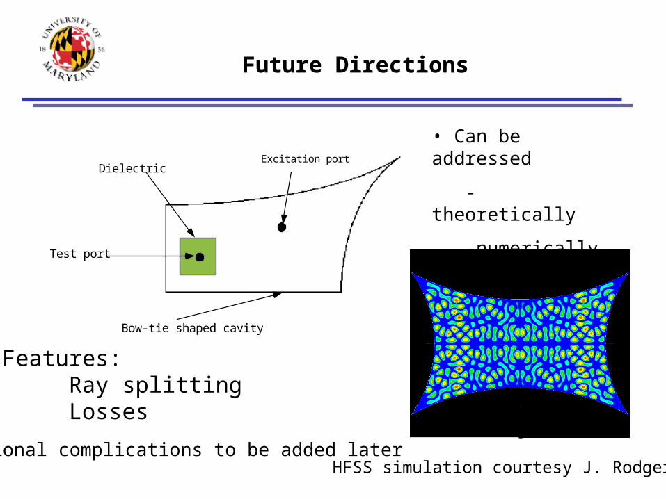
Future Directions

Bow-tie shaped cavity

Dielectric

Test port

Excitation port

• Can be addressed

-theoretically

-numerically

-experimentally

Features:Ray splittingLosses

HFSS simulation courtesy J. RodgersAdditional complications to be added later