statistical quality control a… · sqc are applied to the individual stages separately. unless a...
TRANSCRIPT
Unit V
STATISTICAL QUALITY CONTROL
B. Thilaka
Applied Mathematics

Statistical Quality Control
• Quality Control – Process control & acceptance sampling.
• Tolerance Limits
• Acceptance Sampling
Statistical Quality Control
• Quality- measurable / countable property of a product
• Potency of a drug, breaking strength of a yarn, outside diameter of a ball bearing, number of imperfections in a piece of cloth,….
Quality Control
The concept of quality control in manufacturing was
first advanced by Walter Shewhart
of the Bell Telephone Laboratories. He issued a
memorandum on May 16, 1924 that featured a
sketch of a modern control chart.
1931 - published a book on statistical quality
control, "Economic Control of Quality of
Manufactured Product"
set the tone for subsequent applications of
statistical methods to process control.

Quality Control
Two other Bell Labs statisticians, H.F. Dodge and H.G. Romig spearheaded efforts in applying statistical theory to sampling inspection.
The work of these three pioneers constitutes most of the theory of statistical quality and control
Quality Control - Statistical Process Control
Typical process control techniques:
1. Histograms
2. Check Sheets
3. Pareto Charts
4. Cause and Effect Diagrams
5. Defect Concentration Diagrams
6. Scatter Diagrams
7. Control Charts
Statistical Process Control
The underlying concept of statistical process control is based on a comparison of what is happening today with what happened previously.
Historical data is used to compute the initial control limits. The present data are compared against these initial limits.
Statistical Process Control
• Points that fall outside of the limits are investigated and, perhaps, some will later be discarded.
• If so, the limits would be recomputed and the process repeated.
• This is referred to as Phase I (retrospective anlaysis of data).
• Real-time process monitoring, using the limits from the end of Phase I, is Phase II (prospective monitoring of future data).
Statistical Quality Control
Statistical Quality Control is the process of inspecting enough product from given lots to probabilistically ensure a specified quality level.
Statistical quality control refers to the use of statistical methods in the monitoring and maintaining of the quality of products and services.
Statistical Quality Control
Statistical Process Control is concerned with achieving, maintaining and further improving a good process that produces desirable results reliably and consistently over time.
Applicable to any process that produces data over time according to some underlying statistical model – health care, manufacturing process.
Statistical Quality Control
Why and How do we achieve?
• The production processes are not perfect.
• Hence the output of these processes will not be
perfect – correct and deterministic.
• Successive runs of the same production
process will produce distinct(non-identical)
products (each fingerprint is unique -
variation).
Statistical Quality Control
•Alternately, seemingly similar runs of the
production process will vary, by some
degree, and impart the variation into the
some product characteristics.
•Because of these variations in the products,
we need probabilistic models and robust
statistical techniques to analyze quality of
such products.

Statistical Quality Control
However well a production process is
controlled, these quality measures will vary
from item to item and hence there will be a
probability distribution associated with the
population of such measurements
If all important sources of variations are under control in a production process, then the slight variations among the quality measurements will not cause any serious problem.
Statistical Quality Control
Such a process should produce the same
distribution of quality measurements no matter
when it is sampled, thus ensuring that this is a
“stable system.”
Statistical Quality Control
Variations can be broadly classified into two types.
Chance Variation & Assignable Variation
Chance(common) Variation – Variation in the quality of the product which occurs due to minor but random causes such as slight changes in temperature, pressure, metal hardness.
Statistical Quality Control
Assignable Variation – Variation that occurs due to non-random causes like poor quality raw material, mechanical faults.
A process is said to be in a state of statistical control, if the variability present in the process is confined to chance variation.

Statistical Quality Control
Statistical control is achieved by finding and eliminating all assignable variations.
Once statistical control is achieved, it is essential to maintain the same .
Control charts (Shewart charts) are principally used to detect serious deviations from a state of statistical control when or before(if possible) they occur.
Control charts
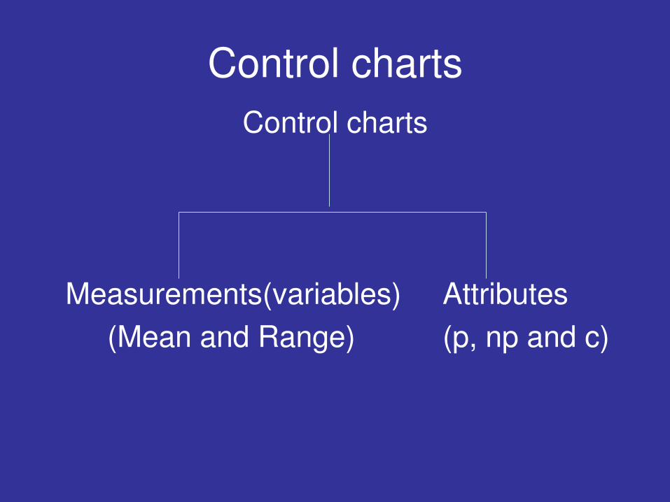
Control charts
Measurements(variables) Attributes
(Mean and Range) (p, np and c)
Control charts
Control charts for measurements:
Observations are measurements
Variables are the quality characteristics of a product that are measurable.
Control charts for attributes:
Observations are count data (the number of defectives in a sample of given data)
Attributes are the quality characteristics of a product that are identified by their presence or absence
Control charts
Control chart consists of
a central line corresponding to the average quality at which the process is to perform
lines corresponding to the upper and lower control limits – limits are chosen so that values falling between them can be attributed to chance, while values falling beyond them are interpreted as indicating a lack of control. (warning limits)
Control charts
Plotting the results obtained from samples taken periodically at frequent intervals can help determine whether the process is under control or any assignable variation has entered the process.
When a sample point falls beyond the control limits or even when the points fall within the control limits if a trend or some other pattern is visible, preventive action is needed.
Control charts
The control limits are used to assess the stability of the process and to identify
unusual events (outliers)
Control charts are thus quite useful both for monitoring if processes get worse and
for testing and verifying improvement ideas
Control charts
A control chart will tell whether a process is out of control, unstable, or unpredictable.
A stable process produces predictable results consistently.
Processes that are “out of control” need to be stabilized before they can be improved.
Control charts
Process is in control:
No points outside the control limits
The number of points above and below the
central line are about the same.
Points are seemingly random above and below
the central line.
Most points are near central line, and only a
few are close to control limits.
Basic Assumption: Central Limit Theorem (Unit II)
Control charts
Process monitoring with control charts is an important component within an overall process evaluation and improvement framework in healthcare.
Control charts
Control chart methods are used extensively in health care
WHERE? HOW?
To verify improvements in the time between insulin injections.
Control charts In cases of epidemiological concerns
such as surgical- site infections, bacteremia, Clostridium difficile toxin-positive stool assays, medical intensive-care-unit (ICU) nosocomial infections, and needlestick injuries.
Can you relate to something else?
EBOLA
Control charts
In many industries, processes will be divided into stages and these principles of SQC are applied to the individual stages separately.
Unless a product is found to meet the specified norms, it will not be permitted to move to the next stage.
This stage-wise SQC scheme ensures that the desired quality level is maintained at all levels.

Control charts
Examples???
Food Processing
Wine-making
The right type of grapes,
Crushing and fermentation,
Processing and aging
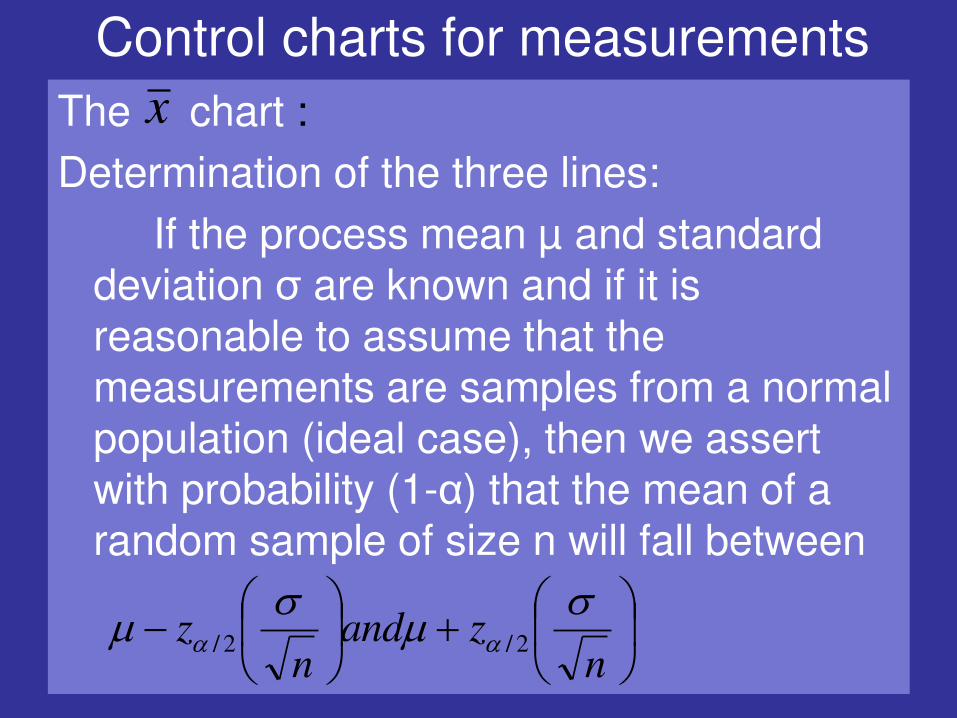
Control charts for measurements
The chart :
Determination of the three lines:
If the process mean µ and standard deviation σ are known and if it is reasonable to assume that the measurements are samples from a normal population (ideal case), then we assert with probability (1-α) that the mean of a random sample of size n will fall between
n
zandn
z 2/2/
x
Control charts for measurements
The chart :
Central line is given by -------------
LCL is given by ------------------
UCL is given by ------------------
x
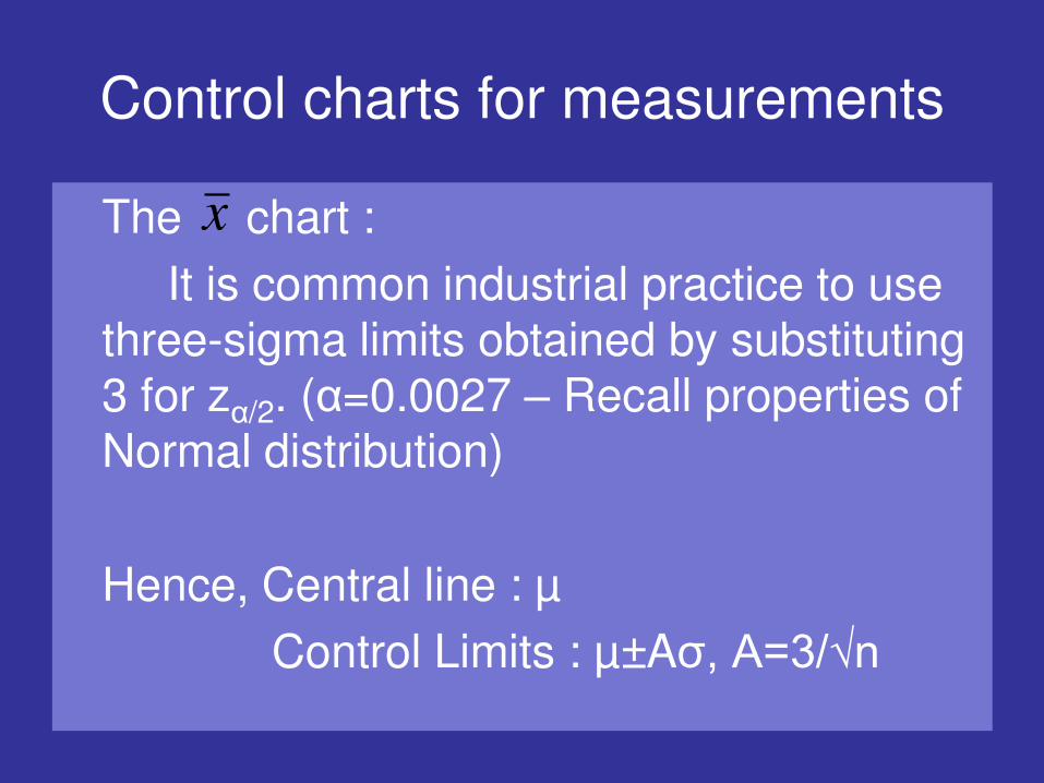
Control charts for measurements
The chart :
It is common industrial practice to use three-sigma limits obtained by substituting 3 for zα/2. (α=0.0027 – Recall properties of Normal distribution)
Hence, Central line : µ
Control Limits : µ±Aσ, A=3/√n
x
Control charts for measurements
If a control chart is being constructed for a
new process, the µ and σ (the population
parameters) will not be known and hence must
be estimated from the sample data.
For establishing control limits, the general rule
of thumb is that at least 30 time points be
sampled before the control limits are
calculated.
For each of the k samples, we compute the
sample mean, the sample variance, and the
range .
Control charts for measurements
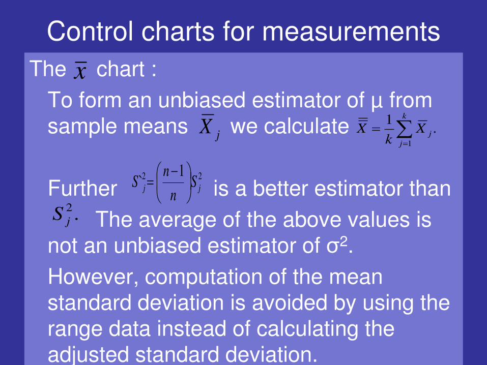
The chart :
To form an unbiased estimator of µ from sample means we calculate
Further is a better estimator than
The average of the above values is not an unbiased estimator of σ2.
However, computation of the mean standard deviation is avoided by using the range data instead of calculating the adjusted standard deviation.
x
jX .1
1
k
j
jXk
X
1
` 22
jj Sn
nS
.2
jS
Control charts for measurements
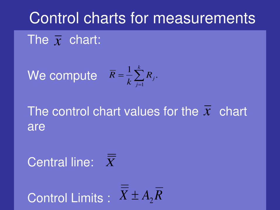
The chart:
We compute
The control chart values for the chart are
Central line:
Control Limits :
.1
1
k
j
jRk
R
x
x
X
RAX 2
Control charts for measurements
The R- chart :
While the chart monitors the central value of the process, the R-chart monitors the variation of the process.
As in the case of the chart, the three values of the R- chart in the various cases are as follows:
x
x

Control charts for measurements
The R- chart :
If the underlying population is normal, with σ known, then
Central line =
UCL =
LCL =
2d
2D
1D
Control charts for measurements
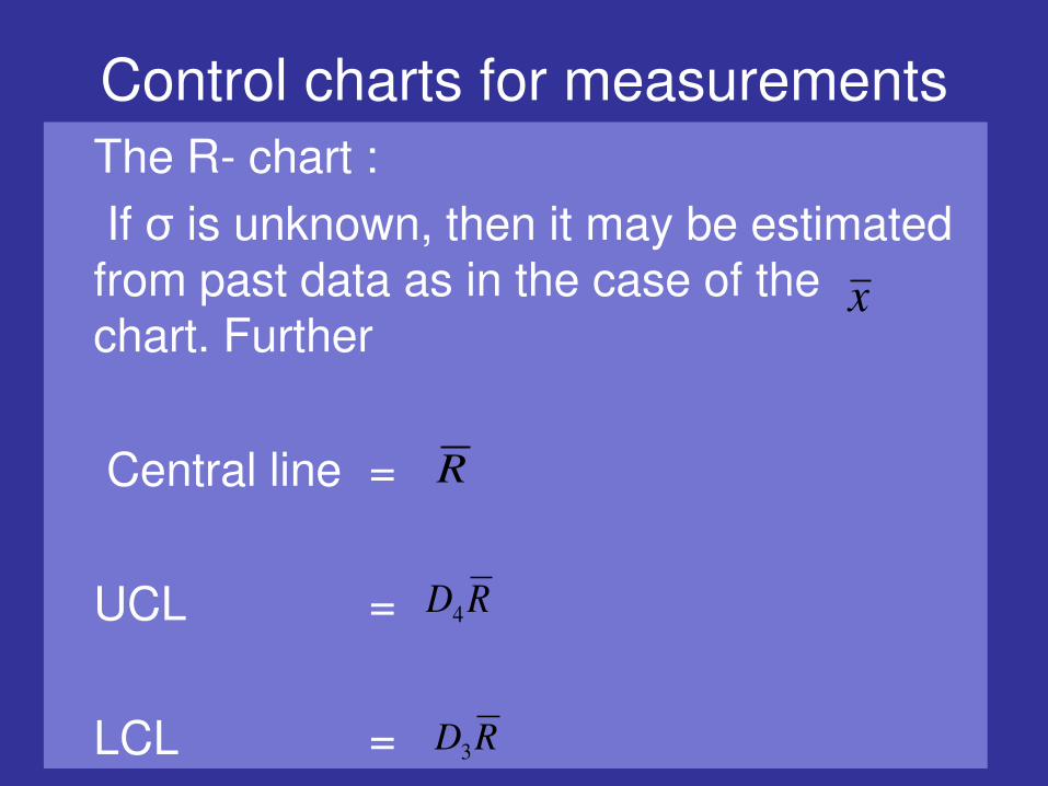
The R- chart :
If σ is unknown, then it may be estimated from past data as in the case of the chart. Further
Central line =
UCL =
LCL =
x
R
RD4
RD3
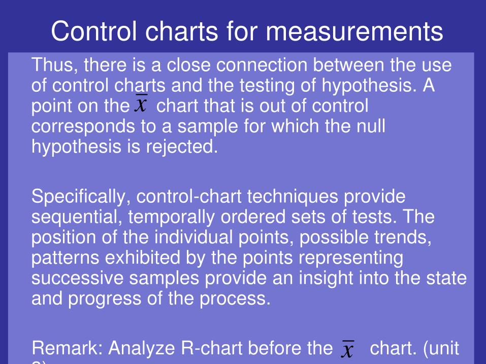
Control charts for measurements Thus, there is a close connection between the use
of control charts and the testing of hypothesis. A point on the chart that is out of control corresponds to a sample for which the null hypothesis is rejected.
Specifically, control-chart techniques provide sequential, temporally ordered sets of tests. The position of the individual points, possible trends, patterns exhibited by the points representing successive samples provide an insight into the state and progress of the process.
Remark: Analyze R-chart before the chart. (unit 3)
x
x
Control charts for measurements
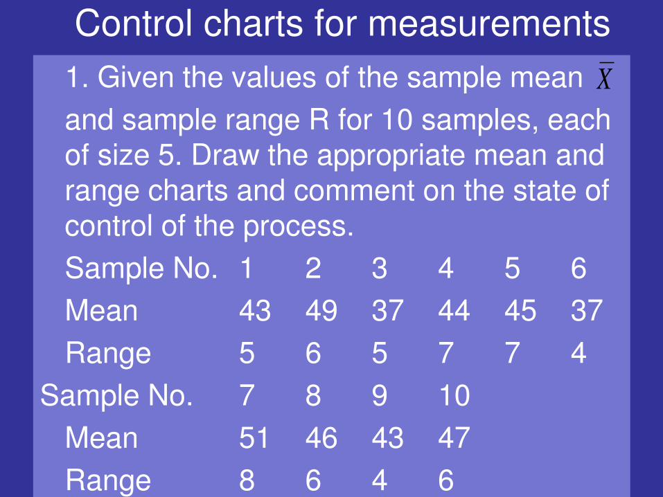
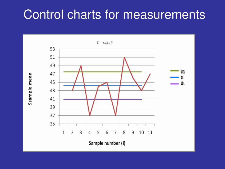
1. Given the values of the sample mean
and sample range R for 10 samples, each of size 5. Draw the appropriate mean and range charts and comment on the state of control of the process.
Sample No. 1 2 3 4 5 6
Mean 43 49 37 44 45 37
Range 5 6 5 7 7 4
Sample No. 7 8 9 10
Mean 51 46 43 47
Range 8 6 4 6
X
Control charts for measurements
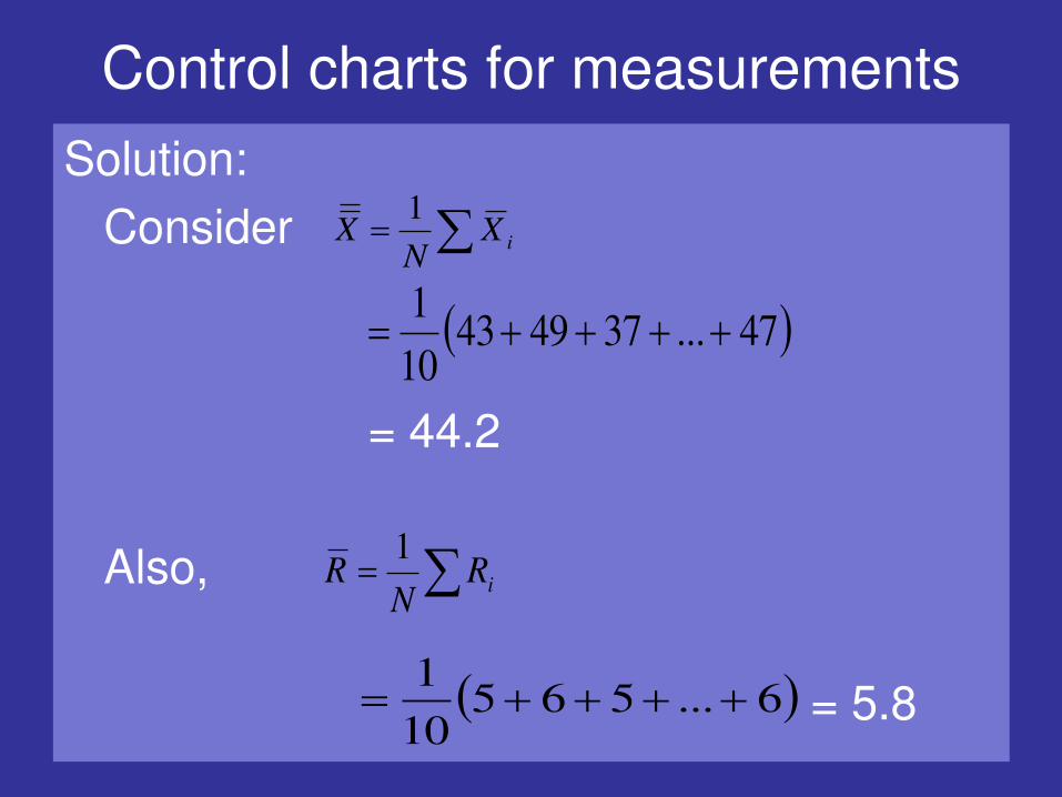
Solution:
Consider
= 44.2
Also,
= 5.8
iXN
X1
47...37494310
1
iRN
R1
6...56510
1
Control charts for measurements
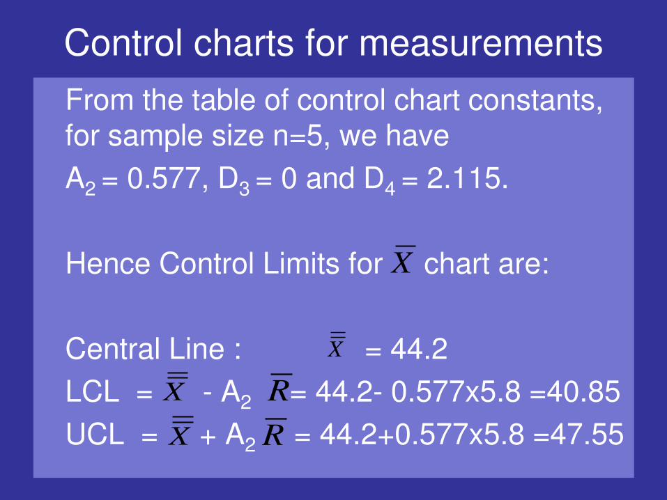
From the table of control chart constants, for sample size n=5, we have
A2 = 0.577, D3 = 0 and D4 = 2.115.
Hence Control Limits for chart are:
Central Line : = 44.2
LCL = - A2 = 44.2- 0.577x5.8 =40.85
UCL = + A2 = 44.2+0.577x5.8 =47.55
X
X
X R
X R

Control charts for measurements
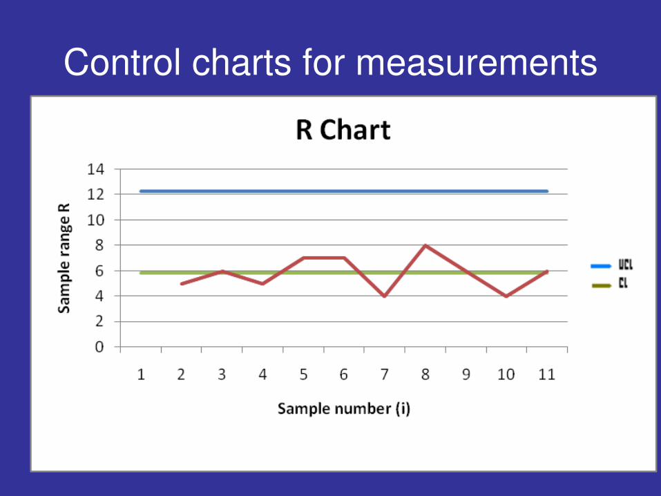
Further, the Control Limits for R chart are:
CL= =5.8
LCL = D3 =0
UCL= D4 =2.115x5.8=12.27.
We now draw the required two control charts
RR
R
Control charts for measurements
Control charts for measurements
Control charts for measurements
State of Control:
Since all the points in the range chart lie
within the control lines, the process is under control as far as the variability of the sample
values is concerned.
However in the mean chart two points lie above
the upper control line and two points lie below
the lower control line. The process is thus not under control as far as the average of the
sample values is concerned.
On the whole, the process is out of control.
Control charts for measurements
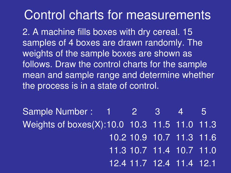
2. A machine fills boxes with dry cereal. 15
samples of 4 boxes are drawn randomly. The
weights of the sample boxes are shown as follows. Draw the control charts for the sample
mean and sample range and determine whether
the process is in a state of control.
Sample Number : 1 2 3 4 5
Weights of boxes(X): 10.0 10.3 11.5 11.0 11.3
10.2 10.9 10.7 11.3 11.6
11.3 10.7 11.4 10.7 11.0
12.4 11.7 12.4 11.4 12.1
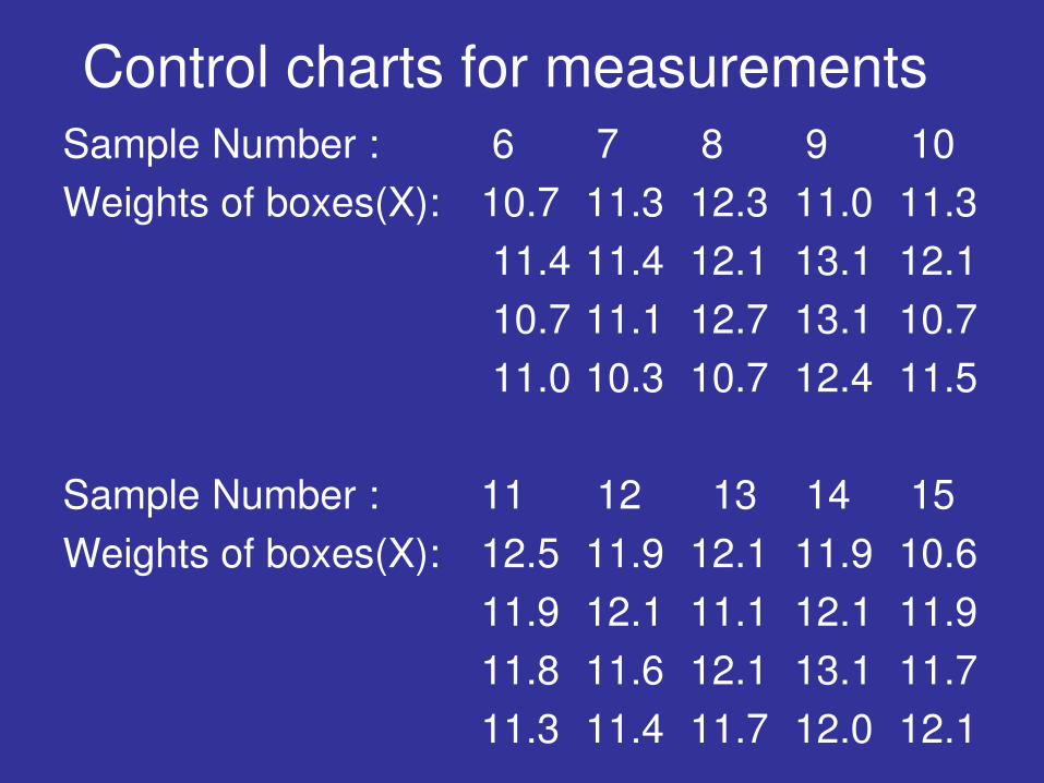
Control charts for measurements
Sample Number : 6 7 8 9 10
Weights of boxes(X): 10.7 11.3 12.3 11.0 11.3
11.4 11.4 12.1 13.1 12.1
10.7 11.1 12.7 13.1 10.7
11.0 10.3 10.7 12.4 11.5
Sample Number : 11 12 13 14 15
Weights of boxes(X): 12.5 11.9 12.1 11.9 10.6
11.9 12.1 11.1 12.1 11.9
11.8 11.6 12.1 13.1 11.7
11.3 11.4 11.7 12.0 12.1
Control charts for measurements
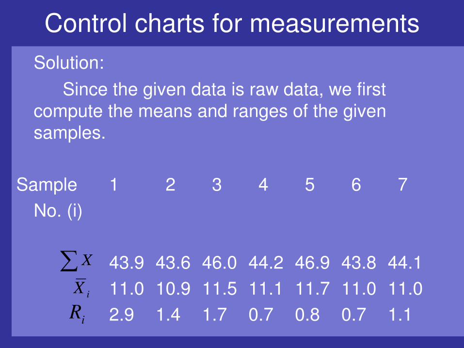
Solution:
Since the given data is raw data, we first
compute the means and ranges of the given samples.
Sample 1 2 3 4 5 6 7
No. (i)
43.9 43.6 46.0 44.2 46.9 43.8 44.1
11.0 10.9 11.5 11.1 11.7 11.0 11.0
2.9 1.4 1.7 0.7 0.8 0.7 1.1
X
iX
iR
Control charts for measurements
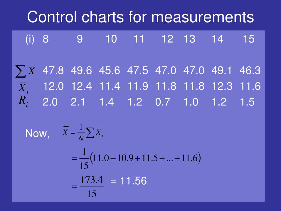
(i) 8 9 10 11 12 13 14 15
47.8 49.6 45.6 47.5 47.0 47.0 49.1 46.3
12.0 12.4 11.4 11.9 11.8 11.8 12.3 11.6
2.0 2.1 1.4 1.2 0.7 1.0 1.2 1.5
Now,
= 11.56
X
iX
iR
iXN
X1
6.11...5.119.100.1115
1
15
4.173
Control charts for measurements
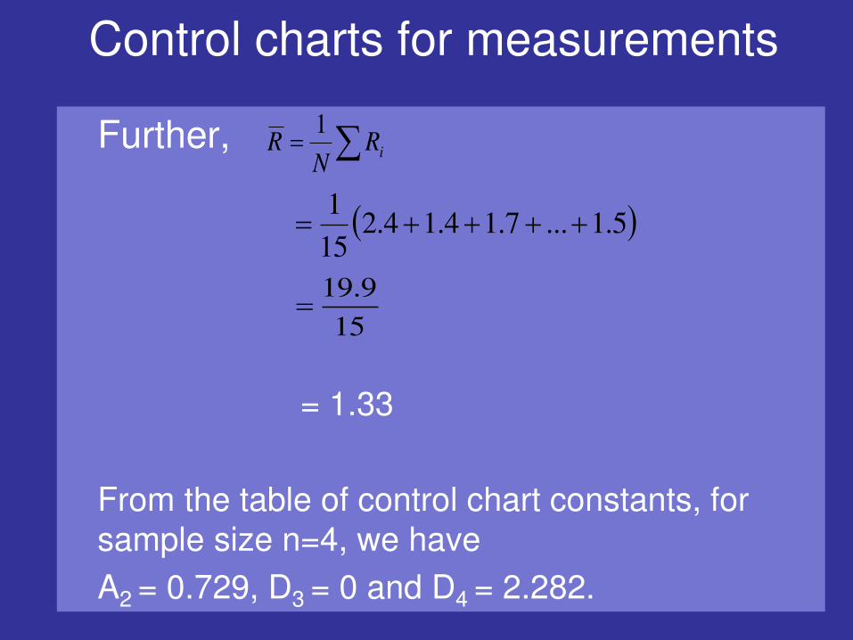
Further,
= 1.33
From the table of control chart constants, for
sample size n=4, we have
A2 = 0.729, D3 = 0 and D4 = 2.282.
iRN
R1
5.1...7.14.14.215
1
15
9.19
Control charts for measurements
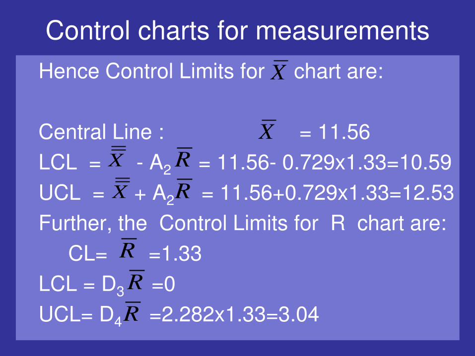
Hence Control Limits for chart are:
Central Line : = 11.56
LCL = - A2 = 11.56- 0.729x1.33=10.59
UCL = + A2 = 11.56+0.729x1.33=12.53
Further, the Control Limits for R chart are:
CL= =1.33
LCL = D3 =0
UCL= D4 =2.282x1.33=3.04
X
X
X
R
R
X
R
R
R
Control charts for measurements
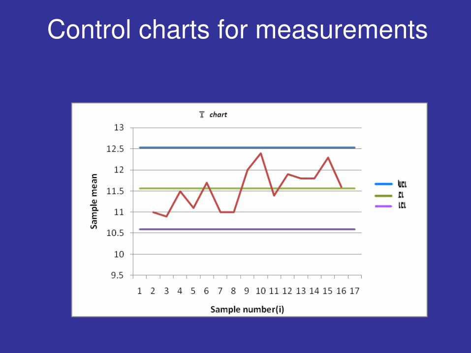
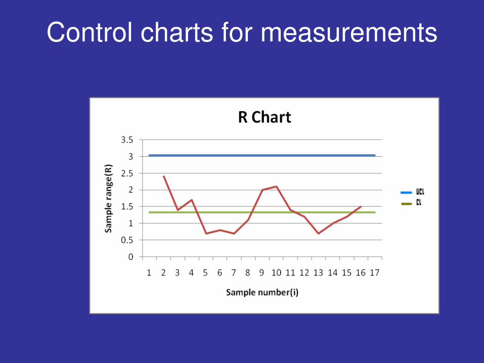
We now draw the required two control charts as given below:
Control charts for measurements
Control charts for measurements

Control charts for measurements
State of Control:
Since all the points lie within the upper and lower control lines in both the mean chart and the R-chart, the process is under control.
Control charts for measurements
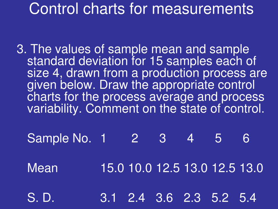
3. The values of sample mean and sample
standard deviation for 15 samples each of size 4, drawn from a production process are given below. Draw the appropriate control charts for the process average and process variability. Comment on the state of control.
Sample No. 1 2 3 4 5 6 Mean 15.0 10.0 12.5 13.0 12.5 13.0 S. D. 3.1 2.4 3.6 2.3 5.2 5.4
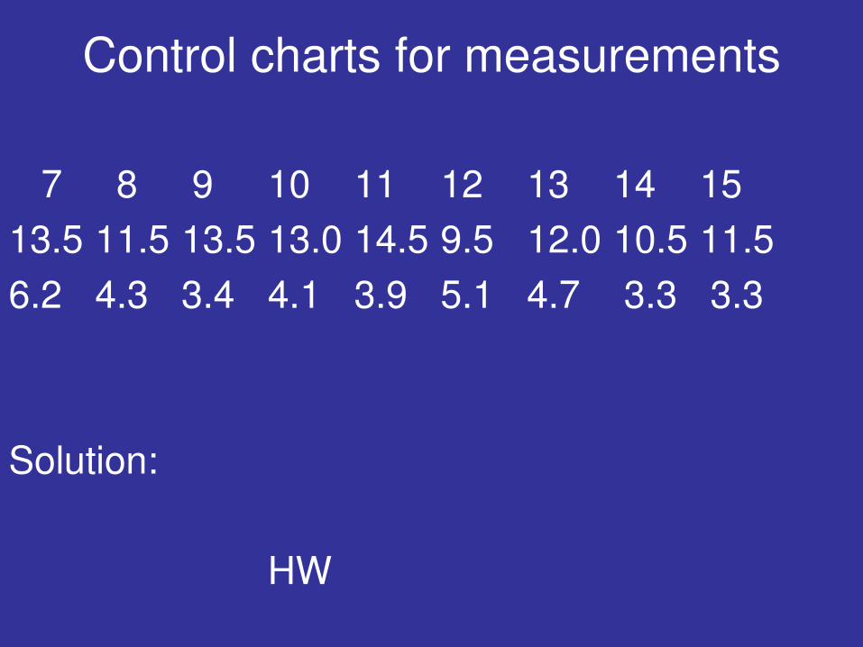
Control charts for measurements
7 8 9 10 11 12 13 14 15
13.5 11.5 13.5 13.0 14.5 9.5 12.0 10.5 11.5
6.2 4.3 3.4 4.1 3.9 5.1 4.7 3.3 3.3
Solution:
HW
Control charts for measurements
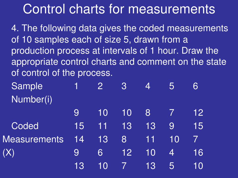
4. The following data gives the coded measurements
of 10 samples each of size 5, drawn from a
production process at intervals of 1 hour. Draw the appropriate control charts and comment on the state
of control of the process.
Sample 1 2 3 4 5 6
Number(i)
9 10 10 8 7 12
Coded 15 11 13 13 9 15
Measurements 14 13 8 11 10 7
(X) 9 6 12 10 4 16
13 10 7 13 5 10
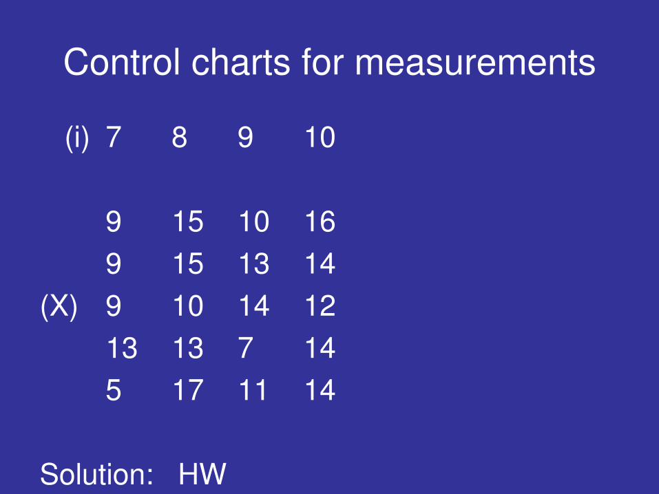
Control charts for measurements
(i) 7 8 9 10
9 15 10 16
9 15 13 14
(X) 9 10 14 12
13 13 7 14
5 17 11 14
Solution: HW
Control charts for attributes
The control charts seen earlier plots quality characteristics that can be measured and expressed numerically. We measure weight, height, position, thickness, etc.
If a particular quality characteristic cannot be represented numerically, or if it is impractical to do so, then using a quality characteristic to sort or classify an item that is inspected into one of two "buckets“ is a good alternate option.
Control charts for attributes
An example of a common quality characteristic classification would be designating units as "conforming units" or "nonconforming units".
Another quality characteristic criteria would be sorting units into "non defective" and "defective" categories.
Quality characteristics of these types are called attributes.
Control charts for attributes
We observe that there is a difference between
"nonconforming to an engineering specification"
and "defective" -- a nonconforming unit may still function fine and be, in fact, not defective at all,
while a part can be defective and not function as
desired.
Examples of quality characteristics that are
attributes
the number of failures in a production run
the proportion of malfunctioning wafers in a lot
Control charts for attributes
Two fundamental control charts for attributes:
Fraction-defective chart called a “p chart”
Number-of –defects chart called a “c chart”
Control charts for attributes
p-chart is a type of control chart used to monitor the proportion of nonconforming units in a sample, where the nonconforming sample proportion is defined as the ratio of the number of nonconforming units to the sample size, n
Control charts for attributes
c-chart is a type of control chart used to monitor "count"-type data, typically total number of nonconformities per unit. It is also occasionally used to monitor the total number of events occurring in a given unit of time.
Control charts for attributes
The c-chart differs from the p-chart in that it accounts for the possibility of more than one nonconformity per inspection unit, and that (unlike the p-chart and u-chart) it requires a fixed sample size.
The p-chart models "pass"/"fail"-type inspection
only, while the c-chart (and u-chart) give the ability to distinguish between (for example) 2 items which fail inspection because of one fault each and the same two items failing inspection with 5 faults each; in the former case, the p-chart will show two non-conformant items, while the c-chart will show 10 faults.
Control charts for attributes
Nonconformities may also be tracked by type or location which can prove helpful in tracking down assignable causes.

Control charts for attributes(p)
Control Limits for fraction-defective chart :
(Link this to the sampling theory of proportions – unit 3)
(To what distribution will we associate this???)
BINOMIAL
(Ultimately, Normal curve approximation)
Control charts for attributes (p)
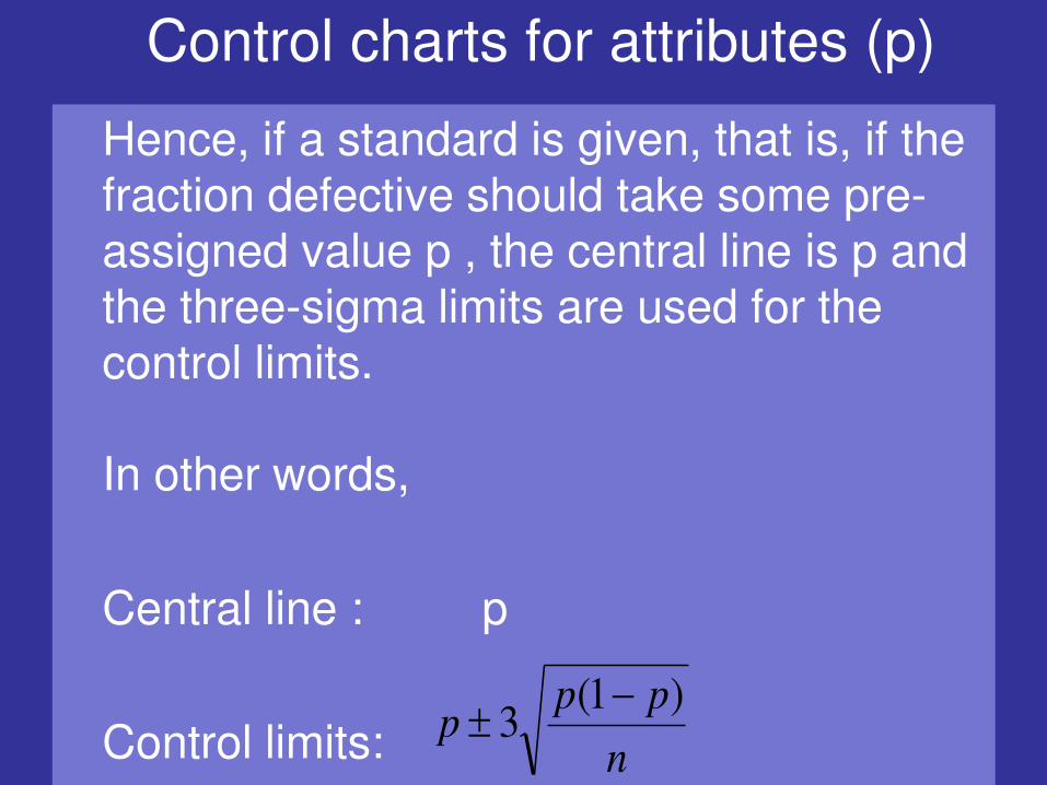
Hence, if a standard is given, that is, if the fraction defective should take some pre-assigned value p , the central line is p and the three-sigma limits are used for the control limits.
In other words,
Central line : p
Control limits:
n
ppp
)1(3
Control charts for attributes (p)
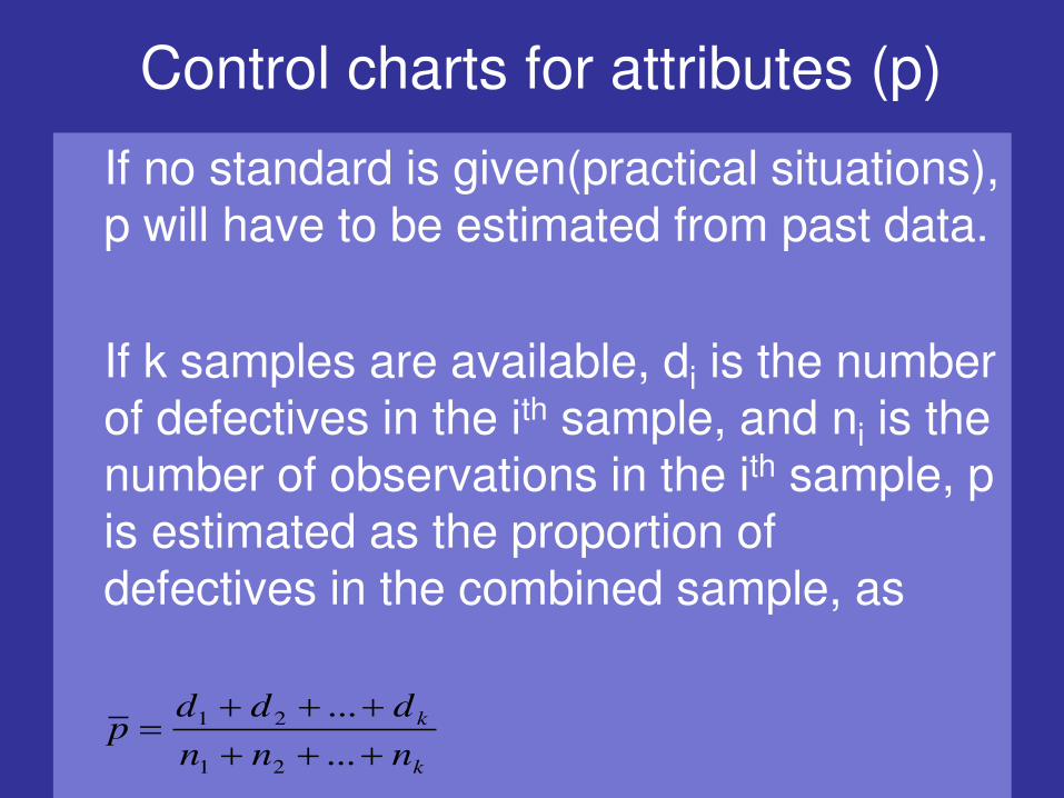
If no standard is given(practical situations), p will have to be estimated from past data.
If k samples are available, di is the number of defectives in the ith sample, and ni is the number of observations in the ith sample, p is estimated as the proportion of defectives in the combined sample, as
k
k
nnn
dddp
...
...
21
21
Control charts for attributes (p)
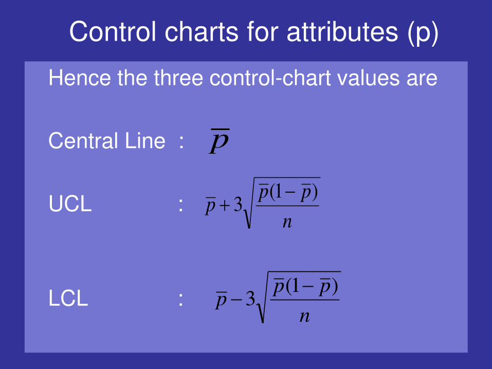
Hence the three control-chart values are
Central Line :
UCL :
LCL :
p
n
ppp
)1(3
n
ppp
)1(3
Control charts for attributes (p)
Note :
1. If p is small, as may often be the case, then,
the LCL may be a negative quantity. In this case, the LCL is assumed to be zero and effectively, only the UCL is used.
2. If the binomial distribution cannot be approximated to a normal curve(when??? – unit I), then and only then the UCL may be obtained directly from the Binomial tables or the Poisson approximation to the Binomial may be used.
Control charts for attributes (np)
The np-chart is a type of control chart used to
monitor the number of nonconforming units in a
sample.
It is an adaptation of the p-chart and used in
situations where it is easier to interpret process
performance in terms of concrete numbers of
units rather than the somewhat more abstract proportion.
Control charts for attributes (np)
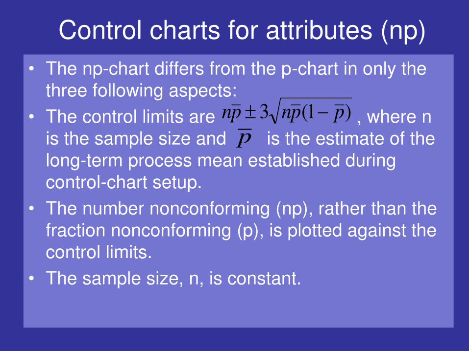
• The np-chart differs from the p-chart in only the
three following aspects:
• The control limits are , where n is the sample size and is the estimate of the
long-term process mean established during
control-chart setup.
• The number nonconforming (np), rather than the
fraction nonconforming (p), is plotted against the
control limits.
• The sample size, n, is constant.
)1(3 ppnpn p
Control charts for attributes (c)
In many situations, it is necessary to control the number of defects in a unit of product, rather than the fraction defective or the number of defectives.
Example:
number of defects per hundred yards in carpeting industry
number of defects per roll in newsprint industry.
Control charts for attributes (c)
Control Limits for no-of-defects chart :
(To what distribution will we associate this???)
POISSON - WHY???
Control charts for attributes (c)
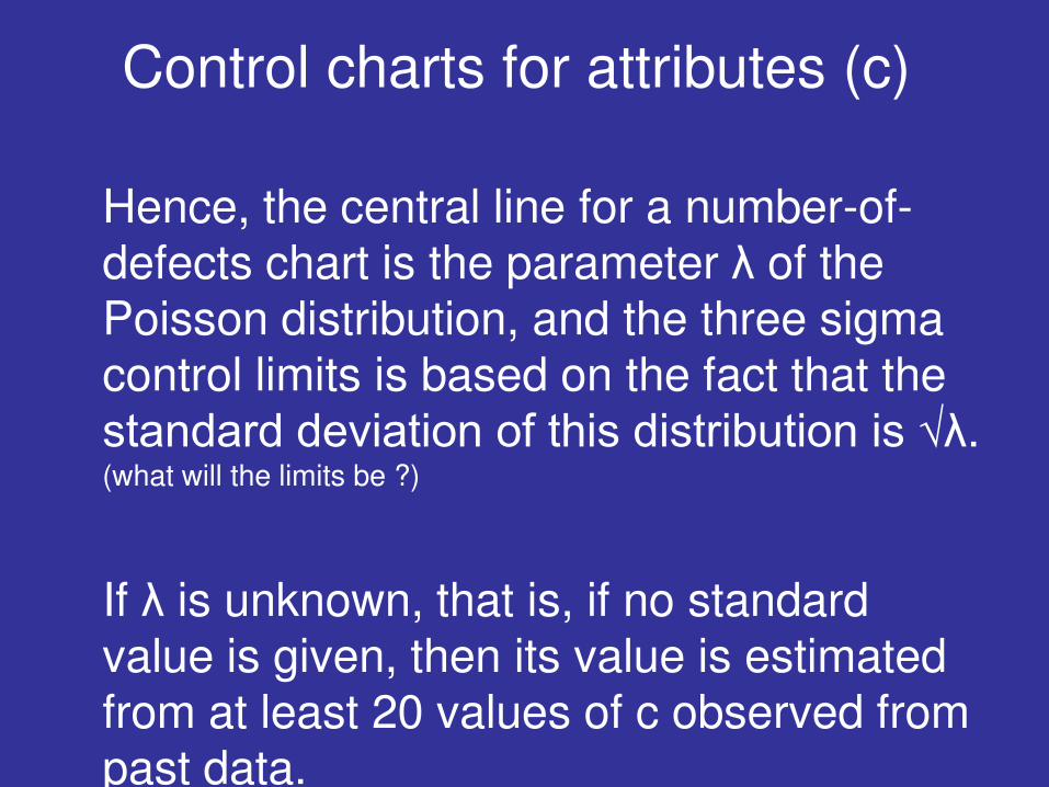
Hence, the central line for a number-of-defects chart is the parameter λ of the Poisson distribution, and the three sigma control limits is based on the fact that the standard deviation of this distribution is √λ. (what will the limits be ?)
If λ is unknown, that is, if no standard value is given, then its value is estimated from at least 20 values of c observed from past data.
Control charts for attributes (c)
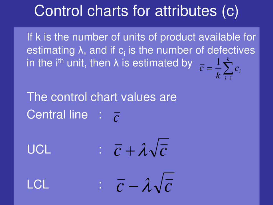
If k is the number of units of product available for
estimating λ, and if ci is the number of defectives
in the ith unit, then λ is estimated by
The control chart values are
Central line :
UCL :
LCL :
k
i
ick
c1
1
c
cc
cc
Control charts for attributes
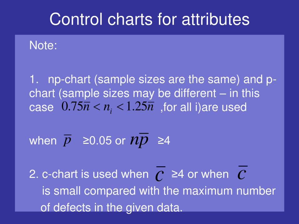
Note:
1. np-chart (sample sizes are the same) and p-
chart (sample sizes may be different – in this
case ,for all i)are used
when ≥0.05 or ≥4
2. c-chart is used when ≥4 or when
is small compared with the maximum number
of defects in the given data.
p pn
c c
nnn i 25.175.0
Control charts for attributes
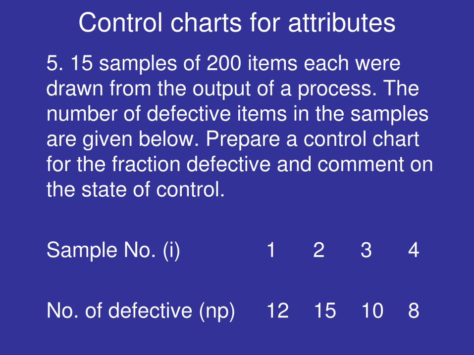
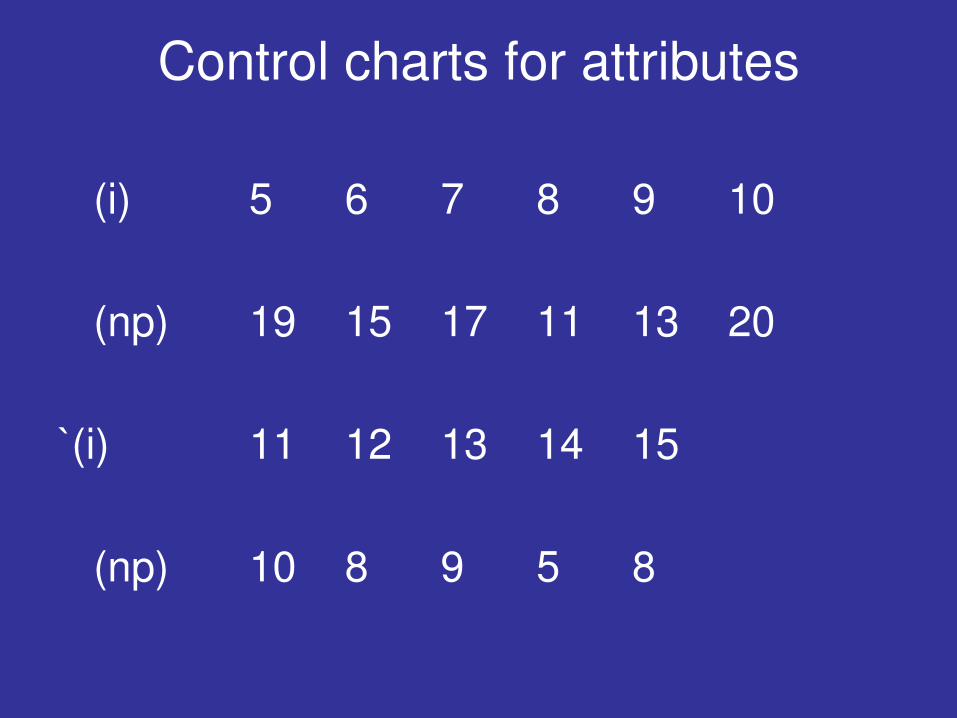
5. 15 samples of 200 items each were drawn from the output of a process. The number of defective items in the samples are given below. Prepare a control chart for the fraction defective and comment on the state of control.
Sample No. (i) 1 2 3 4
No. of defective (np) 12 15 10 8
Control charts for attributes
(i) 5 6 7 8 9 10
(np) 19 15 17 11 13 20
`(i) 11 12 13 14 15
(np) 10 8 9 5 8
Control charts for attributes
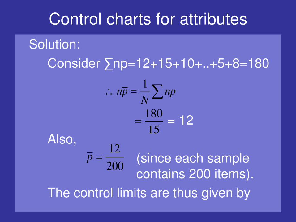
Solution:
Consider ∑np=12+15+10+..+5+8=180
= 12
Also,
(since each sample contains 200 items).
The control limits are thus given by
npN
pn1
15
180
200
12p
Control charts for attributes
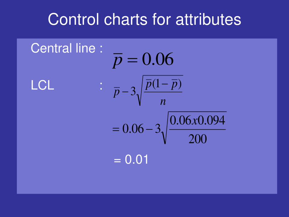
Central line :
LCL :
= 0.01
06.0p
n
ppp
)1(3
200
094.006.0306.0
x
Control charts for attributes
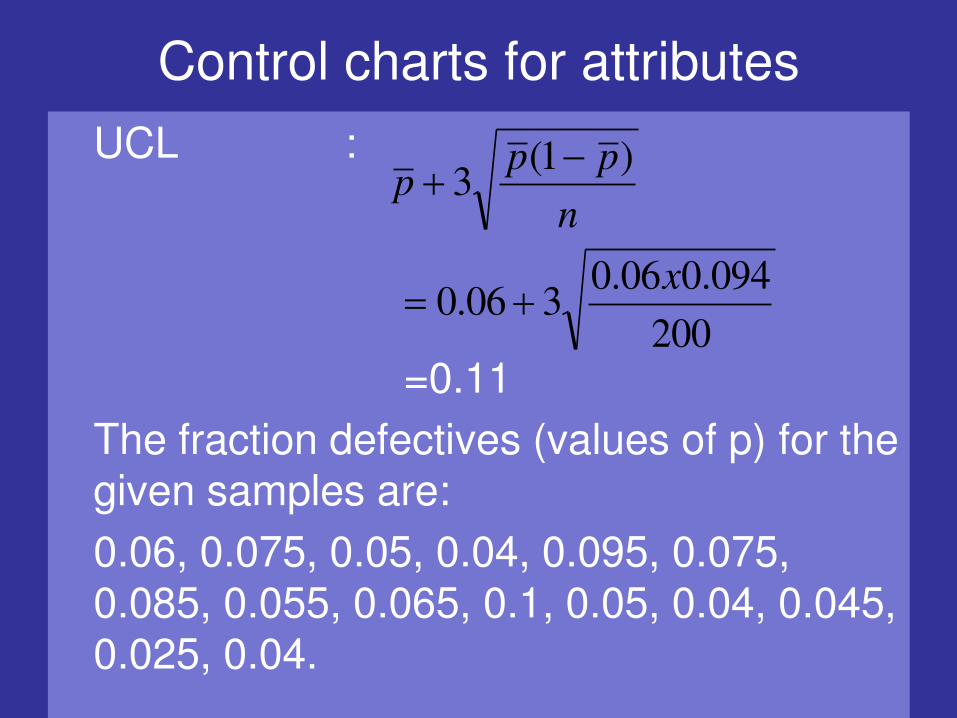
UCL :
=0.11
The fraction defectives (values of p) for the given samples are:
0.06, 0.075, 0.05, 0.04, 0.095, 0.075, 0.085, 0.055, 0.065, 0.1, 0.05, 0.04, 0.045, 0.025, 0.04.
n
ppp
)1(3
200
094.006.0306.0
x
Control charts for attributes

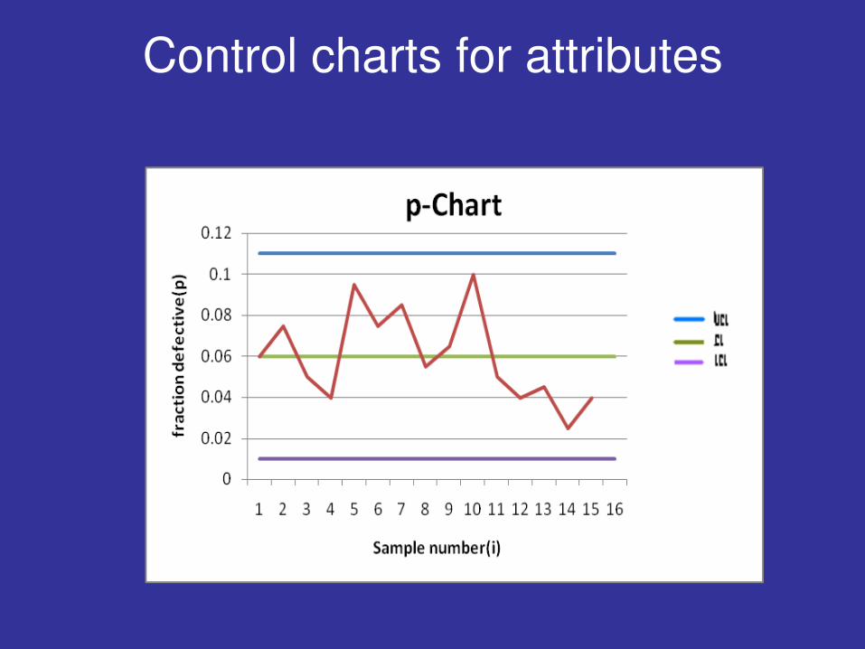
Control charts for attributes
Since all the sample points lie between the LCL and UCL lines, the process is under control.
Control charts for attributes
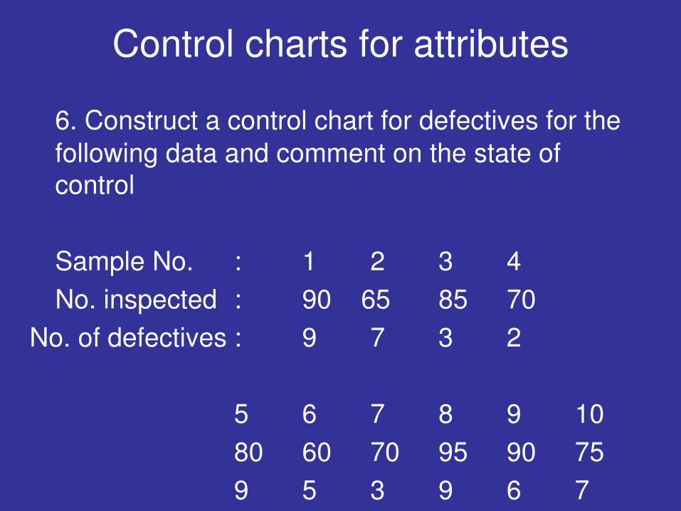
6. Construct a control chart for defectives for the
following data and comment on the state of control
Sample No. : 1 2 3 4
No. inspected : 90 65 85 70
No. of defectives : 9 7 3 2
5 6 7 8 9 10
80 60 70 95 90 75
9 5 3 9 6 7
Control charts for attributes
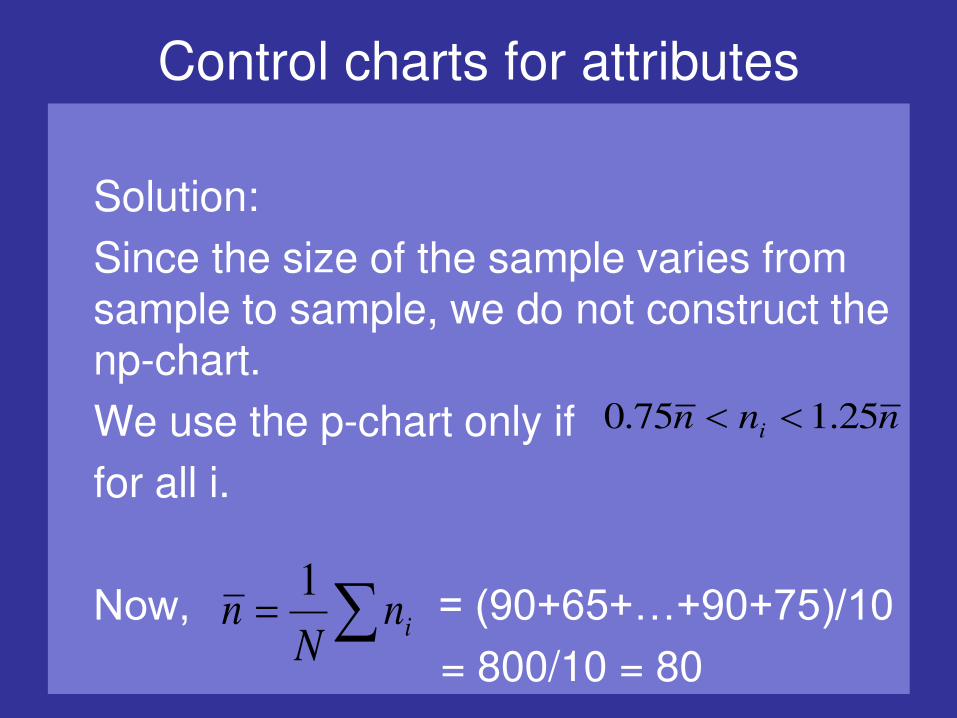
Solution:
Since the size of the sample varies from sample to sample, we do not construct the np-chart.
We use the p-chart only if
for all i.
Now, = (90+65+…+90+75)/10
= 800/10 = 80
nnn i 25.175.0
inN
n1

Control charts for attributes
The values of ni are all between 60 and 100 .
Hence, we now draw the p-chart.
Now, = (Total no. of defectives)/
(Total no. of items inspected)
= 60/800 = 0.075
Hence the control limits are given by
p
Control charts for attributes
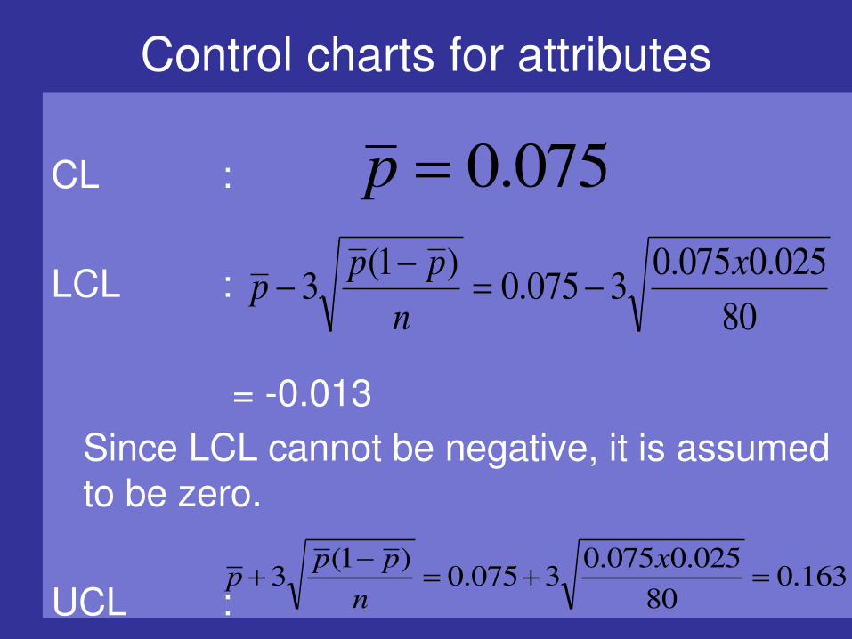
CL :
LCL :
= -0.013
Since LCL cannot be negative, it is assumed to be zero.
UCL :
075.0p
80
025.0075.03075.0
)1(3
x
n
ppp
163.080
025.0075.03075.0
)1(3
x
n
ppp
Control charts for attributes
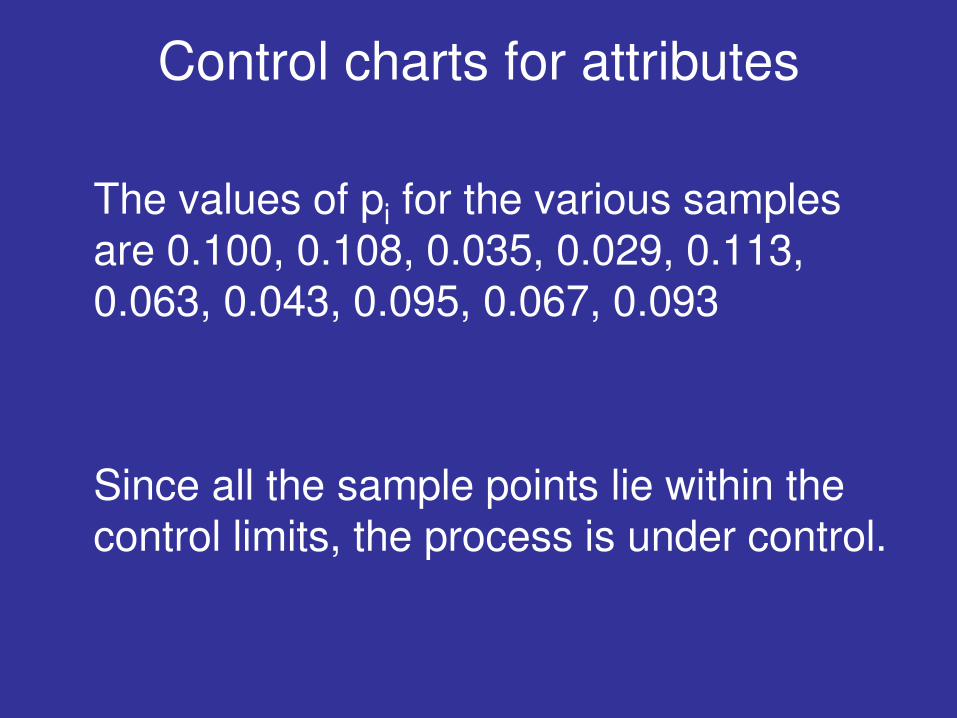
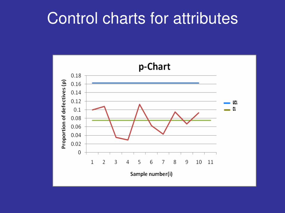
The values of pi for the various samples are 0.100, 0.108, 0.035, 0.029, 0.113, 0.063, 0.043, 0.095, 0.067, 0.093
Since all the sample points lie within the control limits, the process is under control.
Control charts for attributes
Control charts for attributes
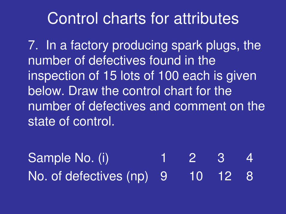
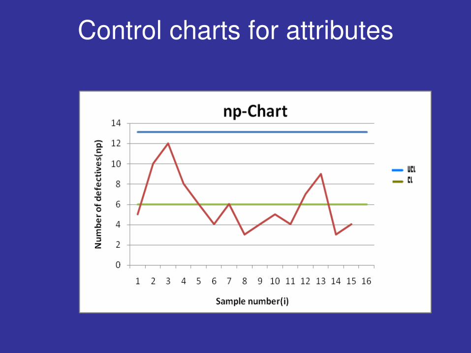
7. In a factory producing spark plugs, the number of defectives found in the inspection of 15 lots of 100 each is given below. Draw the control chart for the number of defectives and comment on the state of control.
Sample No. (i) 1 2 3 4
No. of defectives (np) 9 10 12 8
Control charts for attributes
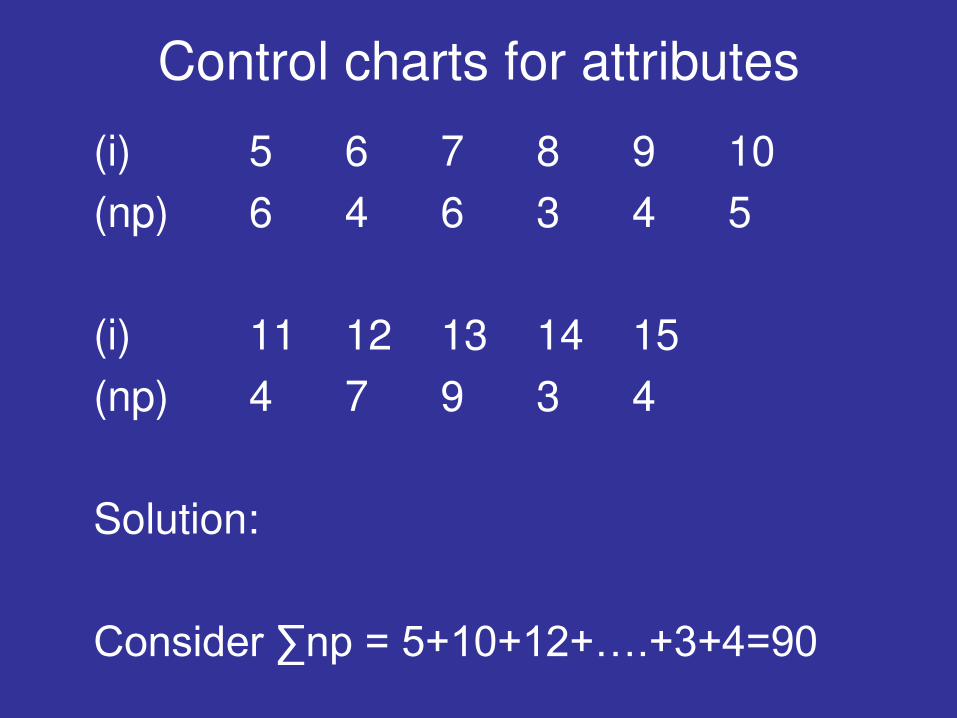
(i) 5 6 7 8 9 10
(np) 6 4 6 3 4 5
(i) 11 12 13 14 15
(np) 4 7 9 3 4
Solution:
Consider ∑np = 5+10+12+….+3+4=90

Control charts for attributes
= 90/15 = 6
and = 6/100 = 0.06 ( since each sample contains 100 items)
The control limits for the np-chart are
CL : = 6
npN
pn1
p
pn
Control charts for attributes
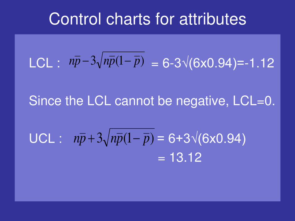
LCL : = 6-3√(6x0.94)=-1.12
Since the LCL cannot be negative, LCL=0.
UCL : = 6+3√(6x0.94) = 13.12
)1(3 ppnpn
)1(3 ppnpn
Control charts for attributes
Control charts for attributes
Since all the sample points lie between the upper and lower control limits, the process is under control.
Control charts for attributes
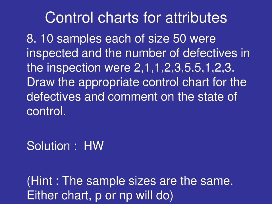
8. 10 samples each of size 50 were inspected and the number of defectives in the inspection were 2,1,1,2,3,5,5,1,2,3. Draw the appropriate control chart for the defectives and comment on the state of control.
Solution : HW
(Hint : The sample sizes are the same. Either chart, p or np will do)
Control charts for attributes
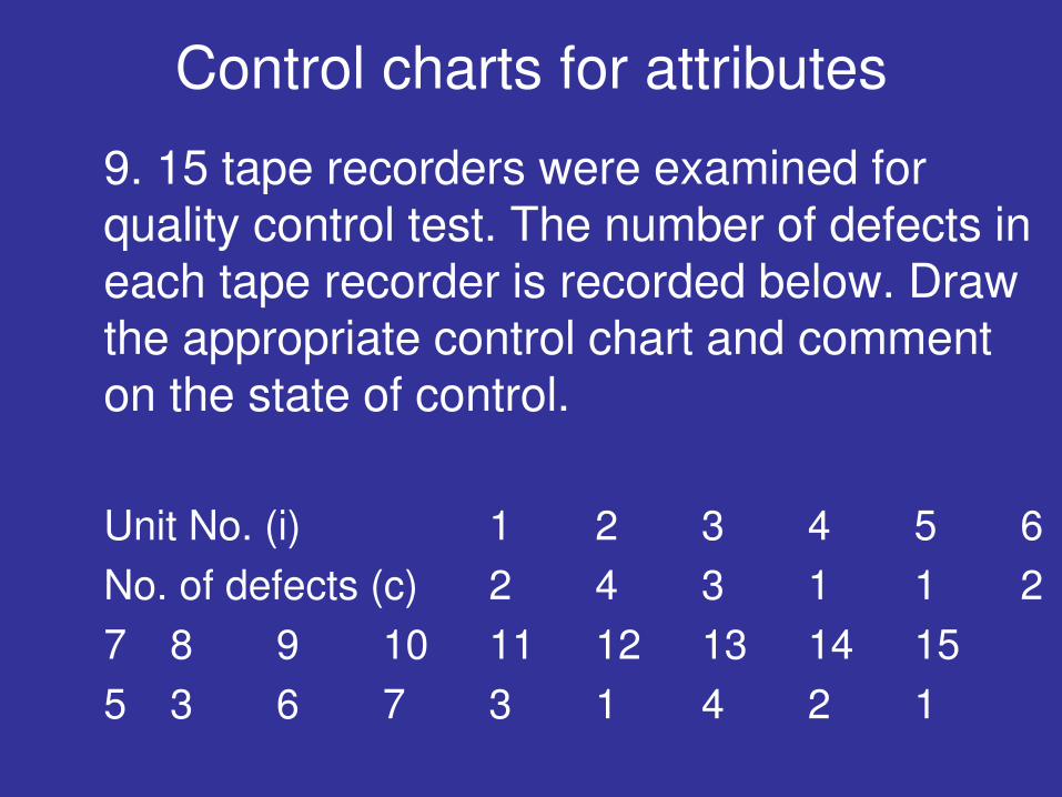
9. 15 tape recorders were examined for quality control test. The number of defects in each tape recorder is recorded below. Draw the appropriate control chart and comment on the state of control.
Unit No. (i) 1 2 3 4 5 6
No. of defects (c) 2 4 3 1 1 2
7 8 9 10 11 12 13 14 15
5 3 6 7 3 1 4 2 1
Control charts for attributes
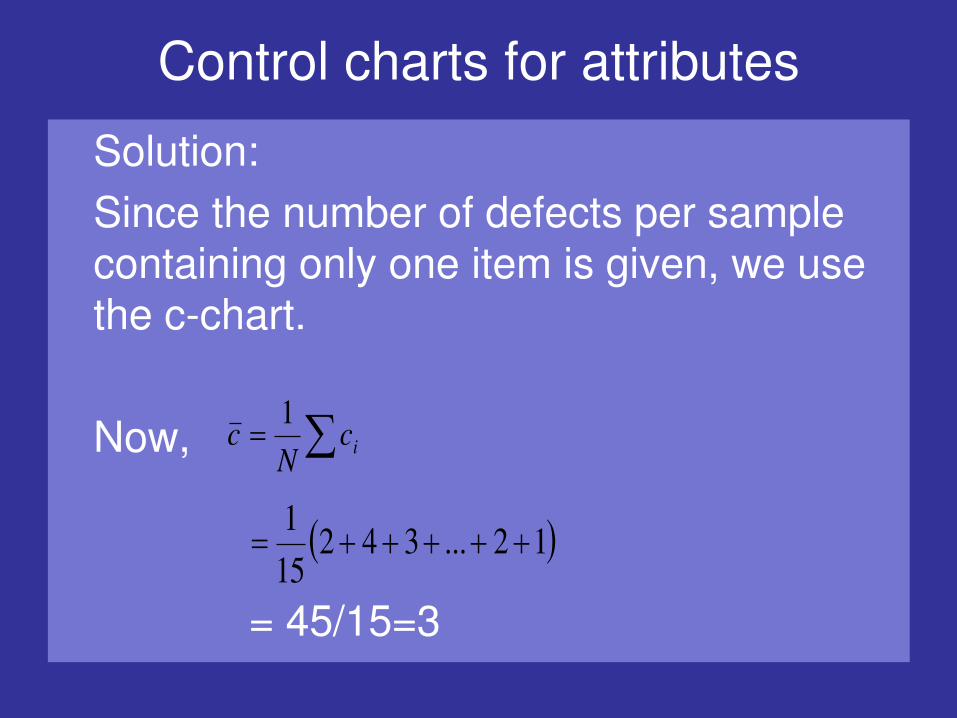
Solution:
Since the number of defects per sample containing only one item is given, we use the c-chart.
Now,
= 45/15=3
icN
c1
12...34215
1

Control charts for attributes
Aside: Observe that even though <4, we use only the c-chart at this point of time.
We now compute the three control limits :
CL : = 3
LCL : = 3-3√3 = -2.20
Since LCL cannot be negative, LCL=0
UCL : = 3+3√3 = 8.20
c
ccc 3
cc 3

Control charts for attributes
Control charts for attributes
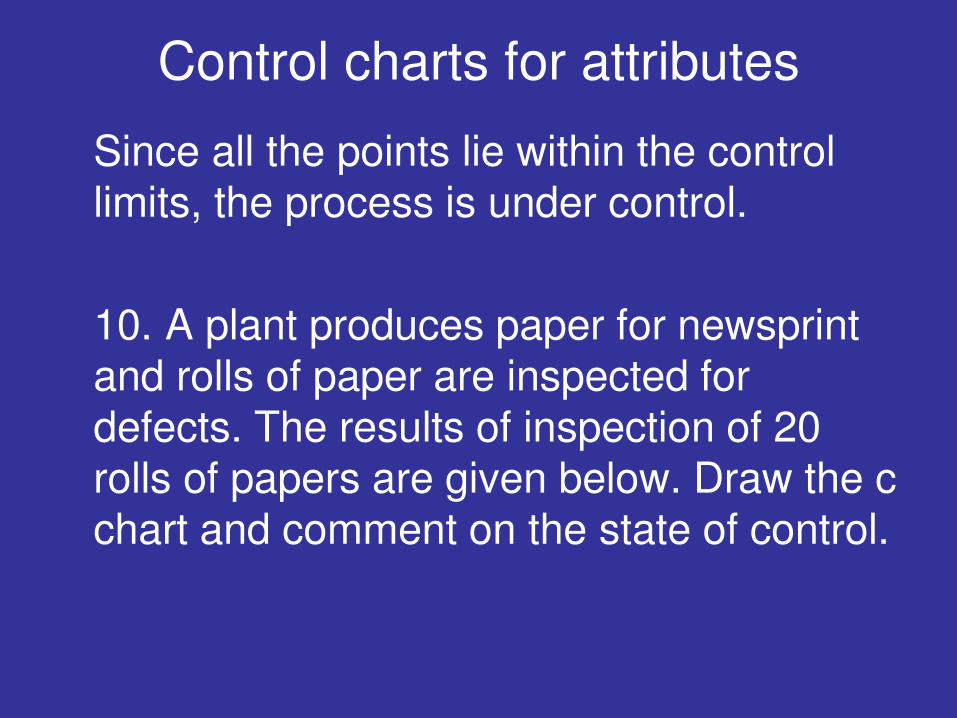
Since all the points lie within the control limits, the process is under control.
10. A plant produces paper for newsprint and rolls of paper are inspected for defects. The results of inspection of 20 rolls of papers are given below. Draw the c chart and comment on the state of control.
Control charts for attributes
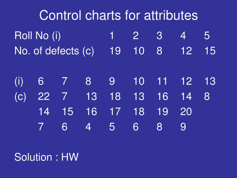
Roll No (i) 1 2 3 4 5
No. of defects (c) 19 10 8 12 15
(i) 6 7 8 9 10 11 12 13
(c) 22 7 13 18 13 16 14 8
14 15 16 17 18 19 20
7 6 4 5 6 8 9
Solution : HW
Tolerance Limits
In quality control, the limiting values between
which measurements must lie if a product is to be accepted is loosely defined as tolerance
limits.
(Contrast this with confidence limits of unit 3)
(Confidence limits are the lower and upper boundaries / values of a confidence interval, that
is, the values which define the range of a
confidence interval).
Tolerance Limits
Recall ”A confidence interval gives an estimated range of values which is likely to include an unknown population parameter, the estimated range being calculated from a given set of sample data.”
If reliable information is available about the distribution underlying the measurement in question, the natural tolerance limits are clearly easily obtained.
Tolerance Limits
In most practical situations, the true values of µ and σ are not known and therefore, the tolerance limits are based on the mean and standard deviation of a random sample.
While in a normal population, µ±1.96σ are the tolerance limits that include 95% of the population, the same cannot be said of for the limits based on sample mean and sample standard deviation.
Tolerance Limits
However, it is possible to determine a constant K so that “one can assert with
(1-α) 100% confidence that the proportion of the population contained between
and is at least P”, the given proportion of the population.
Can you now differentiate between confidence limits(of unit 3) and tolerance limits?
Ksx Ksx
Tolerance Limits
Confidence limits are used to estimate a
parameter of a population.
Tolerance limits are used to indicate between
what limits one can find a certain proportion of the population
Further observe that when n becomes large, the length of a confidence interval approaches zero
while the tolerance limits approach the
corresponding values of the population.

Acceptance Sampling
Acceptance sampling is an important field of statistical quality control that was popularized by Dodge and Romig and originally applied by the U.S. military to the testing of bullets during World War II. If every bullet was tested in advance, no bullets would be left to ship. If, on the other hand, none were tested, malfunctions might occur in the field of battle, with potentially disastrous results.
Acceptance Sampling
Dodge reasoned that a sample should be picked at random from the lot, and on the basis of information that was yielded by the sample, a decision should be made regarding the disposition of the lot. In general, the decision is either to accept or reject the lot. This process is called Lot
Acceptance Sampling or just Acceptance Sampling.
Acceptance Sampling
Acceptance sampling is "the middle of the road"
approach between no inspection and 100% inspection. There are two major classifications of
acceptance plans: by attributes ("go, no-go") and
by variables. The attribute case is the most
common for acceptance sampling.
The main purpose of acceptance sampling is to
decide whether or not the lot is likely to be
acceptable, not to estimate the quality of the lot.
Acceptance Sampling
Acceptance sampling is employed when one or
several of the following hold:
Testing is destructive
The cost of 100% inspection is very high
100% inspection takes too long
This procedure is equivalent to a test of the null
hypothesis that the proportion defective p in the
lot equals some specified value p0 against the
alternative that it equals p1, where p1>p0.
(One tailed test- WHY?? -up for discussion)
Acceptance Sampling
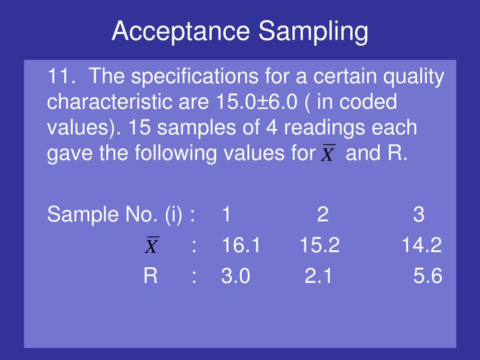
11. The specifications for a certain quality characteristic are 15.0±6.0 ( in coded values). 15 samples of 4 readings each gave the following values for and R.
Sample No. (i) : 1 2 3
: 16.1 15.2 14.2
R : 3.0 2.1 5.6
X
X
Acceptance Sampling
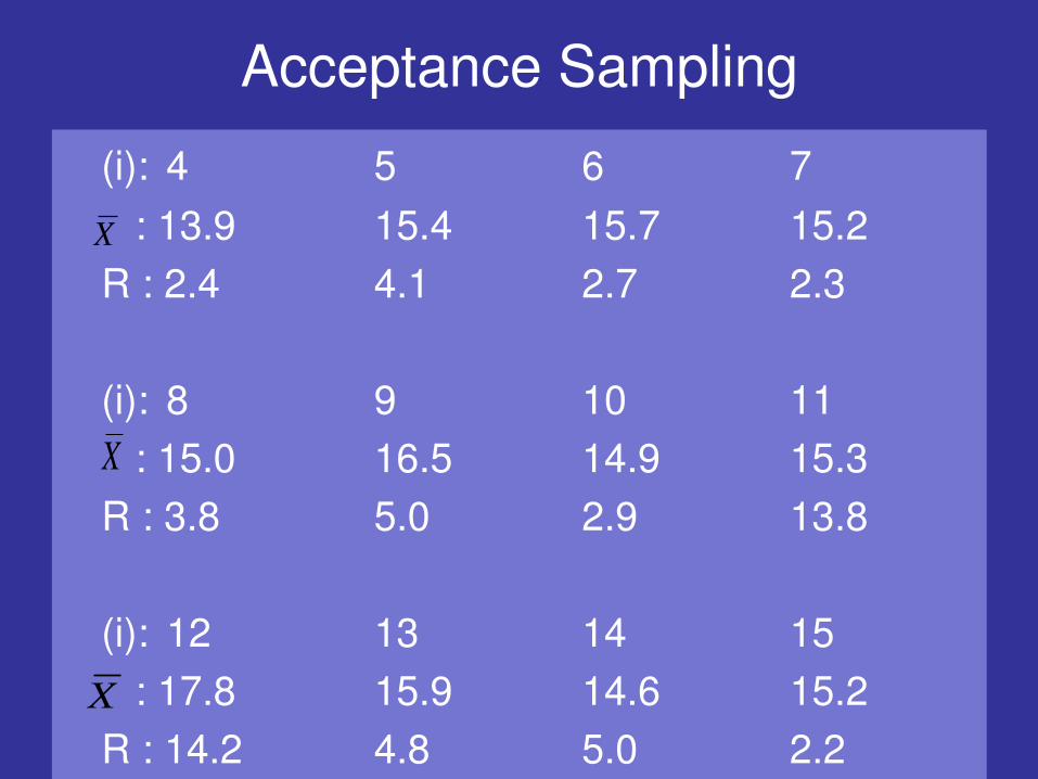
(i): 4 5 6 7
: 13.9 15.4 15.7 15.2
R : 2.4 4.1 2.7 2.3
(i): 8 9 10 11
: 15.0 16.5 14.9 15.3
R : 3.8 5.0 2.9 13.8
(i): 12 13 14 15
: 17.8 15.9 14.6 15.2
R : 14.2 4.8 5.0 2.2
X
X
X
Acceptance Sampling
Compute the control limits for and R-charts using the above data for all the samples. Hence examine if the process is in control. If not, remove the doubtful samples and recompute the values of and . After testing the state of control, estimate the tolerance limits and find if the process will meet the required specifications.
X
X
R
Acceptance Sampling
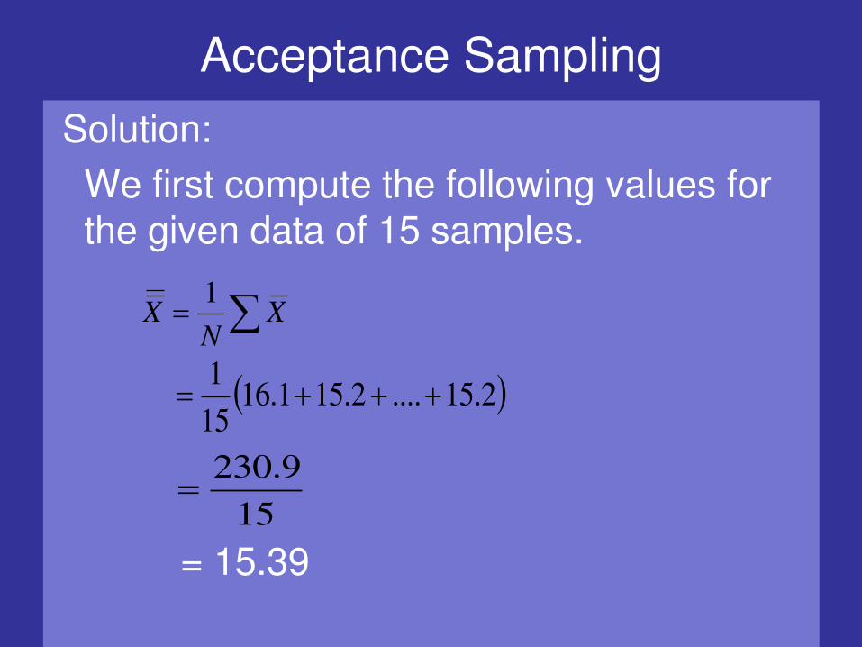
Solution:
We first compute the following values for the given data of 15 samples.
= 15.39
XN
X1
2.15....2.151.1615
1
15
9.230
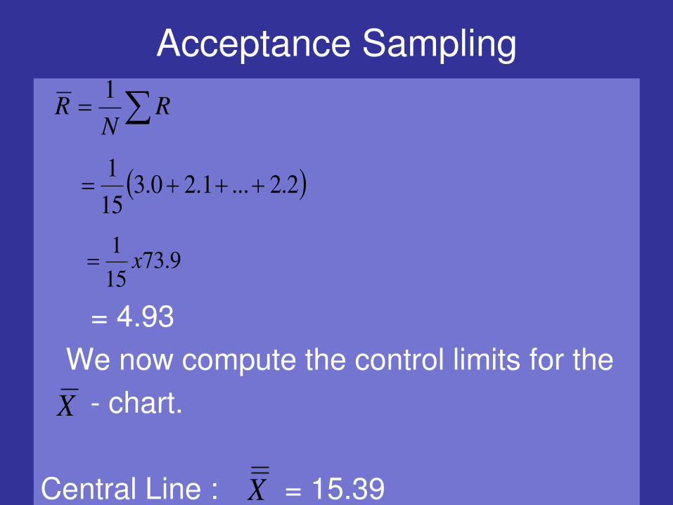
Acceptance Sampling
= 4.93
We now compute the control limits for the
- chart.
Central Line : = 15.39
RN
R1
2.2...1.20.315
1
9.7315
1x
X
X
Acceptance Sampling
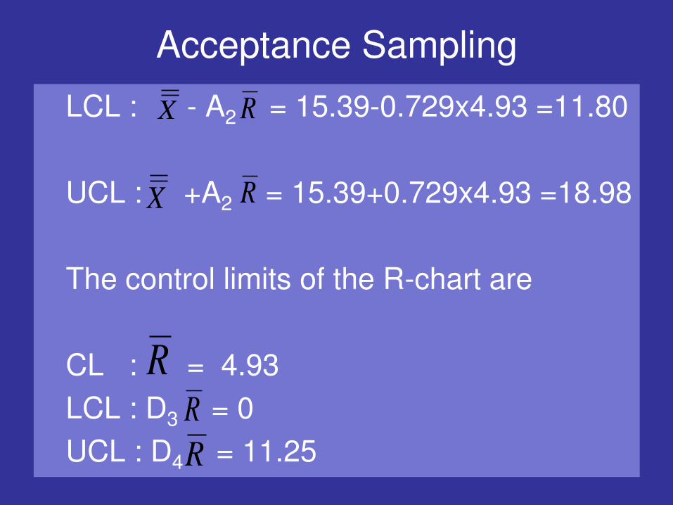
LCL : - A2 = 15.39-0.729x4.93 =11.80
UCL : +A2 = 15.39+0.729x4.93 =18.98
The control limits of the R-chart are
CL : = 4.93
LCL : D3 = 0
UCL : D4 = 11.25
X R
X R
RR
R
Acceptance Sampling
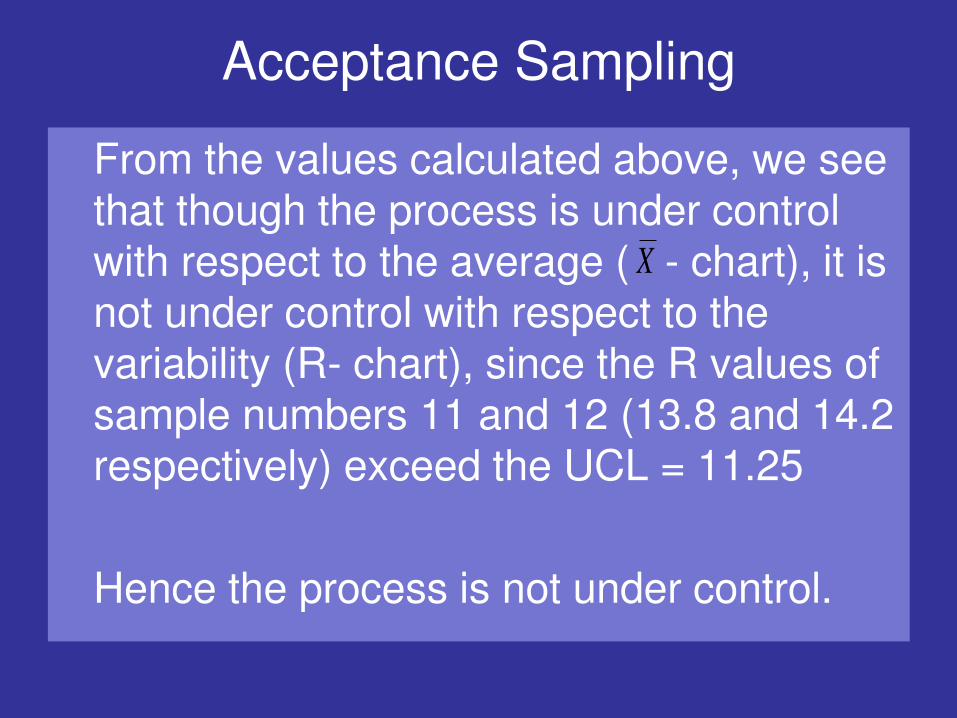
From the values calculated above, we see that though the process is under control with respect to the average ( - chart), it is not under control with respect to the variability (R- chart), since the R values of sample numbers 11 and 12 (13.8 and 14.2 respectively) exceed the UCL = 11.25
Hence the process is not under control.
X
Acceptance Sampling
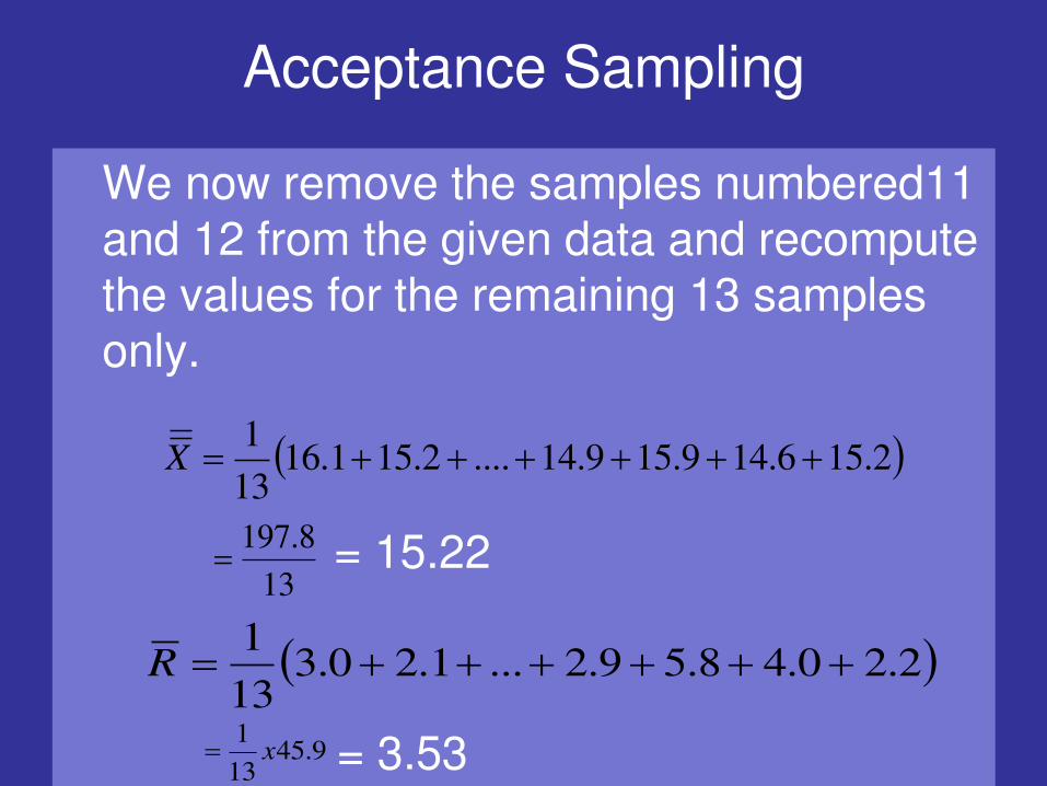
We now remove the samples numbered11 and 12 from the given data and recompute the values for the remaining 13 samples only.
= 15.22
= 3.53
2.156.149.159.14....2.151.1613
1X
13
8.197
2.20.48.59.2...1.20.313
1R
9.4513
1x
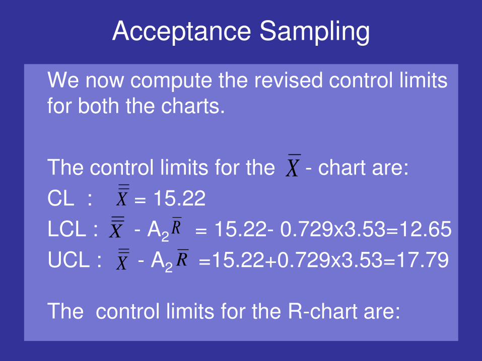
Acceptance Sampling
We now compute the revised control limits for both the charts.
The control limits for the - chart are:
CL : = 15.22
LCL : - A2 = 15.22- 0.729x3.53=12.65
UCL : - A2 =15.22+0.729x3.53=17.79
The control limits for the R-chart are:
X
X
X R
RX
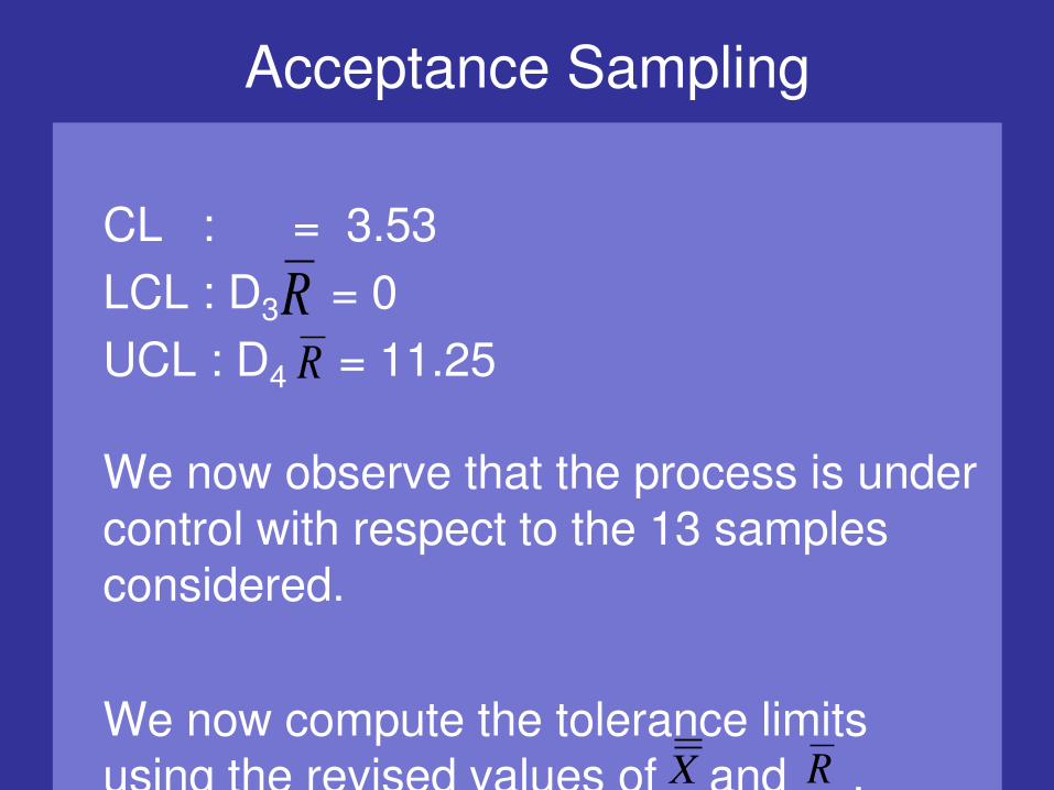
Acceptance Sampling
CL : = 3.53
LCL : D3 = 0
UCL : D4 = 11.25
We now observe that the process is under control with respect to the 13 samples considered.
We now compute the tolerance limits using the revised values of and .
RR
RX

Acceptance Sampling
The tolerance limits are given by :
Thus the required tolerance limits are (10.08, 20.36).
Since these tolerance limits lie within the specification limits (9.0,21.0), the process meets the required specifications.
2
3
d
RX
14.522.15059.2
53.3322.15
x
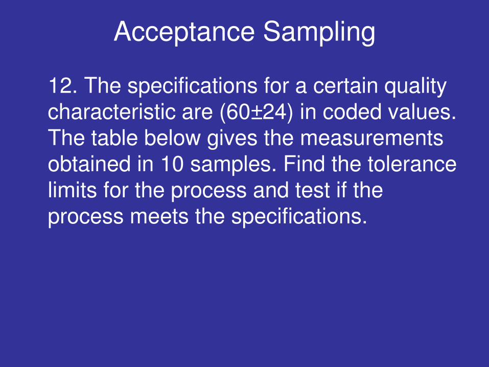
Acceptance Sampling
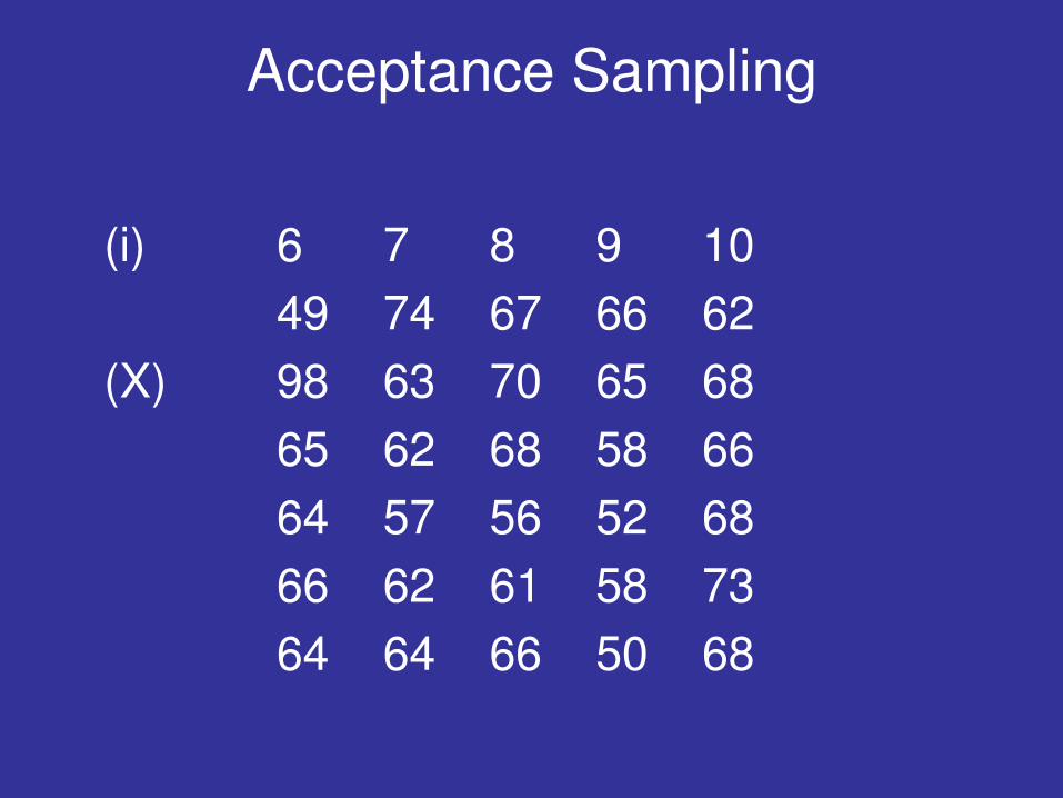
12. The specifications for a certain quality characteristic are (60±24) in coded values. The table below gives the measurements obtained in 10 samples. Find the tolerance limits for the process and test if the process meets the specifications.
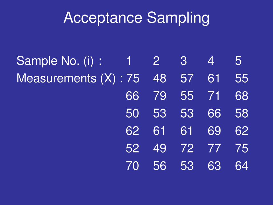
Acceptance Sampling
Sample No. (i) : 1 2 3 4 5
Measurements (X) : 75 48 57 61 55
66 79 55 71 68
50 53 53 66 58
62 61 61 69 62
52 49 72 77 75
70 56 53 63 64
Acceptance Sampling
(i) 6 7 8 9 10
49 74 67 66 62
(X) 98 63 70 65 68
65 62 68 58 66
64 57 56 52 68
66 62 61 58 73
64 64 66 50 68
Acceptance Sampling
Solution : HW
(Hint: In control, does not meet the specifications – under discussion)