statistics 240: nonparametric and robust methods stark/teach/s240/notes/...statistics 240:...
TRANSCRIPT
Statistics 240: Nonparametric and RobustMethods
Philip B. Stark
Department of Statistics
University of California, Berkeley
www.stat.berkeley.edu/∼stark
ROUGH DRAFT NOTES—WORK IN PROGRESS!
Last edited 10 November 2010
1

Course Website:
http://statistics.berkeley.edu/~stark/Teach/S240/F10
2

Example: Effect of treatment in a randomized controlled
experiment
11 pairs of rats, each pair from the same litter.
Randomly—by coin tosses—put one of each pair into “en-
riched” environment; other sib gets ”normal” environment.
After 65 days, measure cortical mass (mg).
treatment 689 656 668 660 679 663 664 647 694 633 653control 657 623 652 654 658 646 600 640 605 635 642difference 32 33 16 6 21 17 64 7 89 -2 11
How should we analyze the data?
(Cartoon of [?]. See also [?] and [?, pp. 498ff]. The experiment had 3 levels, not 2,
and there were several trials.)
3
Informal Hypotheses
Null hypothesis: treatment has “no effect.”
Alternative hypothesis: treatment increases cortical mass.
Suggests 1-sided test for an increase.
4

Test contenders
• 2-sample Student t-test:
mean(treatment) - mean(control)
pooled estimate of SD of difference of means
• 1-sample Student t-test on the differences:
mean(differences)
SD(differences)/√
11
Better, since littermates are presumably more homoge-
neous.
• Permutation test using t-statistic of differences: same
statistic, different way to calculate P -value. Even better?
5
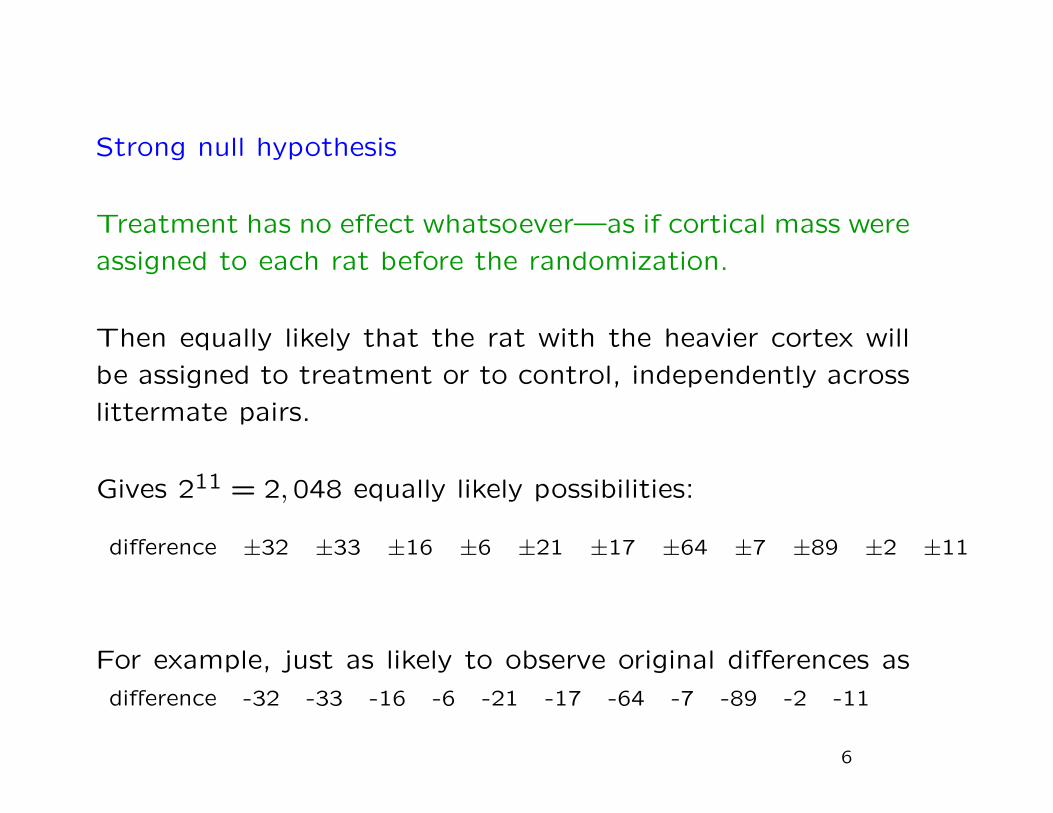
Strong null hypothesis
Treatment has no effect whatsoever—as if cortical mass were
assigned to each rat before the randomization.
Then equally likely that the rat with the heavier cortex will
be assigned to treatment or to control, independently across
littermate pairs.
Gives 211 = 2,048 equally likely possibilities:
difference ±32 ±33 ±16 ±6 ±21 ±17 ±64 ±7 ±89 ±2 ±11
For example, just as likely to observe original differences as
difference -32 -33 -16 -6 -21 -17 -64 -7 -89 -2 -11
6
Weak null hypothesis
On average across pairs, treatment makes no difference.
7
Alternatives
Individual’s response depends only on that individual’s assign-
ment
Special cases: shift, scale, etc.
Interactions/Interference: my response could depend on whether
you are assigned to treatment or control.
8
Assumptions of the tests
• 2-sample t-test: masses are iid sample from normal dis-tribution, same unknown variance, same unknown mean.Tests weak null hypothesis (plus normality, independence,non-interference, etc.).
• 1-sample t-test on the differences: mass differences areiid sample from normal distribution, unknown variance,zero mean. Tests weak null hypothesis (plus normality,independence, non-interference, etc.)
• Permutation test: Randomization fair, independent acrosspairs. Tests strong null hypothesis.
Assumptions of the permutation test are true by design:That’s how treatment was assigned.
9
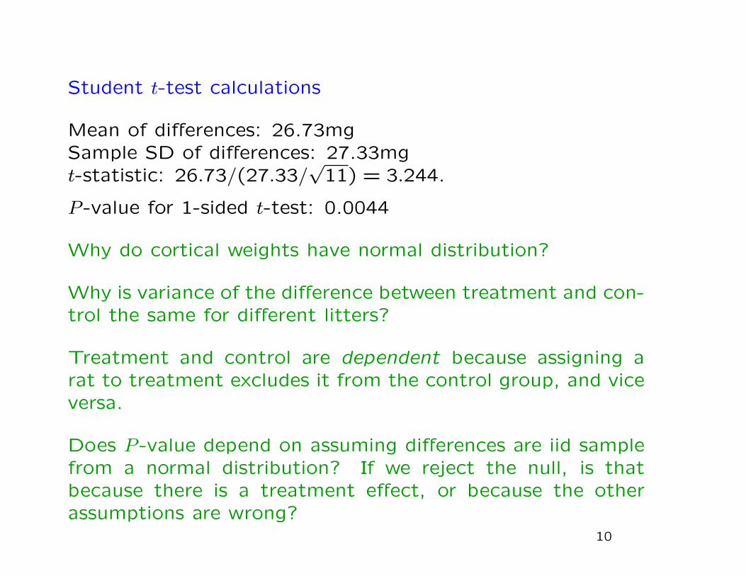
Student t-test calculations
Mean of differences: 26.73mgSample SD of differences: 27.33mgt-statistic: 26.73/(27.33/
√11) = 3.244.
P -value for 1-sided t-test: 0.0044
Why do cortical weights have normal distribution?
Why is variance of the difference between treatment and con-trol the same for different litters?
Treatment and control are dependent because assigning arat to treatment excludes it from the control group, and viceversa.
Does P -value depend on assuming differences are iid samplefrom a normal distribution? If we reject the null, is thatbecause there is a treatment effect, or because the otherassumptions are wrong?
10
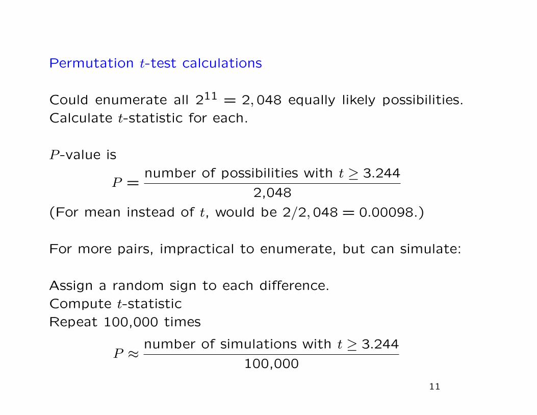
Permutation t-test calculations
Could enumerate all 211 = 2,048 equally likely possibilities.
Calculate t-statistic for each.
P -value is
P =number of possibilities with t ≥ 3.244
2,048
(For mean instead of t, would be 2/2,048 = 0.00098.)
For more pairs, impractical to enumerate, but can simulate:
Assign a random sign to each difference.
Compute t-statistic
Repeat 100,000 times
P ≈number of simulations with t ≥ 3.244
100,000
11

Calculations
simPermuTP <- function(z, iter) # P.B. Stark, www.stat.berkeley.edu/~stark 5/14/07# simulated P-value for 1-sided 1-sample t-test under the# randomization model.
n <- length(z)ts <- mean(z)/(sd(z)/sqrt(n)) # t test statisticsum(replicate(iter, zp <- z*(2*floor(runif(n)+0.5)-1);
tst <- mean(zp)/(sd(zp)/sqrt(n));(tst >= ts)
)
)/itersimPermuTP(diffr, 100000)0.0011
(versus 0.0044 for Student’s t distribution)
12
Other tests: sign test, Wilcoxon signed-rank test
Sign test: Count pairs where treated rat has heavier cortex,i.e., where difference is positive.
Under strong null, distribution of the number of positive dif-ferences is Binomial(11, 1/2). Like number of heads in 11independent tosses of a fair coin. (Assumes no ties w/i pairs.)
P -value is chance of 10 or more heads in 11 tosses of a faircoin: 0.0059.
Only uses signs of differences, not information that only thesmallest absolute difference was negative.
Wilcoxon signed-rank test uses information about the order-ing of the differences: rank the absolute values of the dif-ferences, then give them the observed signs and sum them.Null distribution: assign signs at random and sum.
13
Still more tests, for other alternatives
All the tests we’ve seen here are sensitive to shifts–the alter-
native hypothesis is that treatment increases response (cor-
tical mass).
There are also nonparametric tests that are sensitive to other
treatment effects, e.g., treatment increases the variability of
the response.
And there are tests for whether treatment has any effect at
all on the distribution of the responses.
You can design a test statistic to be sensitive to any change
that interests you, then use the permutation distribution to
get a P -value (and simulation to approximate that P -value).
14
Silliness
Treat ordinal data (e.g., Likert scale) as if measured on a
linear scale; use Student t-test.
Maybe not so silly for large samples. . .
t-test asymptotically distribution-free.
How big is big?
15
Back to Rosenzweig et al.
Actually had 3 treatments: enriched, standard, deprived.
Randomized 3 rats per litter into the 3 treatments, indepen-
dently across n litters.
How should we analyze these data?
16
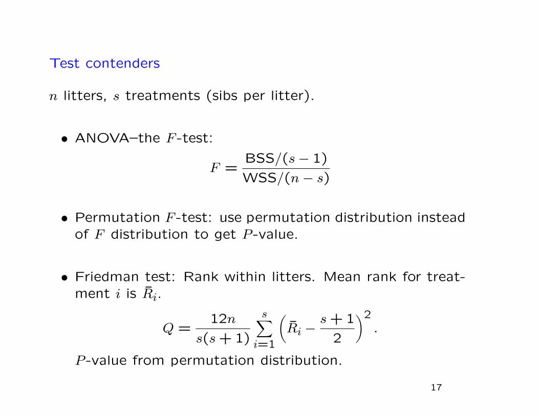
Test contenders
n litters, s treatments (sibs per litter).
• ANOVA–the F -test:
F =BSS/(s− 1)
WSS/(n− s)
• Permutation F -test: use permutation distribution insteadof F distribution to get P -value.
• Friedman test: Rank within litters. Mean rank for treat-ment i is Ri.
Q =12n
s(s+ 1)
s∑i=1
(Ri −
s+ 1
2
)2.
P -value from permutation distribution.
17
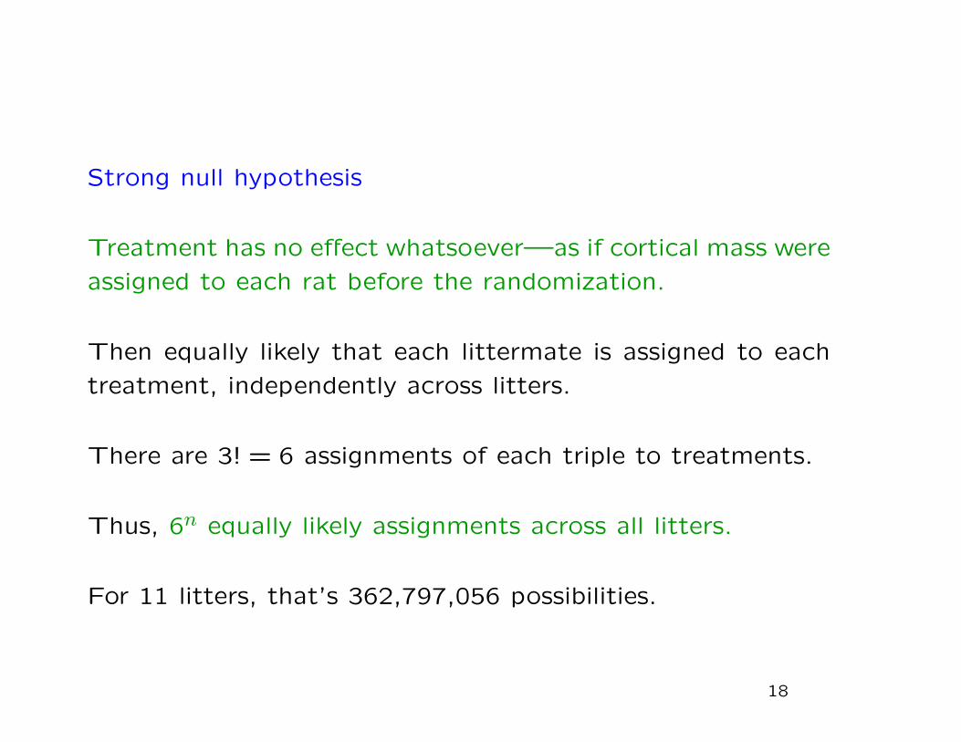
Strong null hypothesis
Treatment has no effect whatsoever—as if cortical mass were
assigned to each rat before the randomization.
Then equally likely that each littermate is assigned to each
treatment, independently across litters.
There are 3! = 6 assignments of each triple to treatments.
Thus, 6n equally likely assignments across all litters.
For 11 litters, that’s 362,797,056 possibilities.
18
Weak null hypothesis
The average cortical weight for all three treatment groups
are equal. On average across triples, treatment makes no
difference.
19
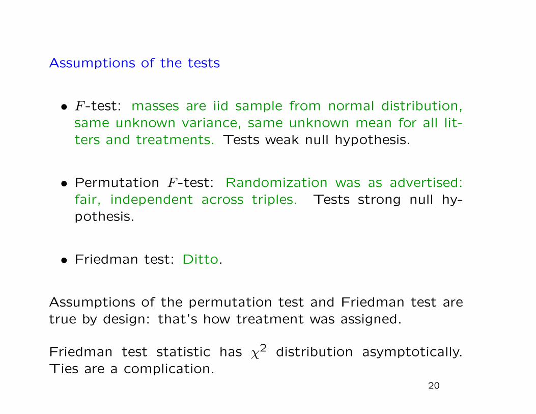
Assumptions of the tests
• F -test: masses are iid sample from normal distribution,same unknown variance, same unknown mean for all lit-ters and treatments. Tests weak null hypothesis.
• Permutation F -test: Randomization was as advertised:fair, independent across triples. Tests strong null hy-pothesis.
• Friedman test: Ditto.
Assumptions of the permutation test and Friedman test aretrue by design: that’s how treatment was assigned.
Friedman test statistic has χ2 distribution asymptotically.Ties are a complication.
20
F -test assumptions–reasonable?
Why do cortical weights have normal distribution for each
litter and for each treatment?
Why is the variance of cortical weights the same for different
litters?
Why is the variance of cortical weights the same for different
treatments?
21
Is F a good statistic for this alternative?
F (and Friedman statistic) sensitive to differences among the
mean responses for each treatment group, no matter what
pattern the differences have.
But the treatments and the responses can be ordered: we
hypothesize that more stimulation produces greater cortical
mass.
deprived =⇒ normal =⇒ enrichedlow mass =⇒ medium mass =⇒ high mass
Can we use that to make a more sensitive test?
22
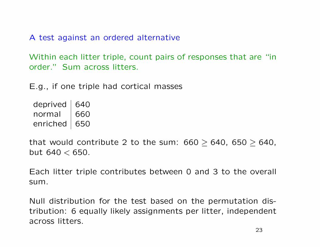
A test against an ordered alternative
Within each litter triple, count pairs of responses that are “inorder.” Sum across litters.
E.g., if one triple had cortical masses
deprived 640normal 660enriched 650
that would contribute 2 to the sum: 660 ≥ 640, 650 ≥ 640,but 640 < 650.
Each litter triple contributes between 0 and 3 to the overallsum.
Null distribution for the test based on the permutation dis-tribution: 6 equally likely assignments per litter, independentacross litters.
23
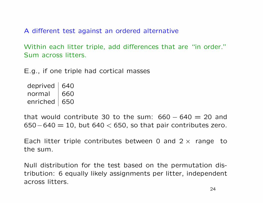
A different test against an ordered alternative
Within each litter triple, add differences that are “in order.”Sum across litters.
E.g., if one triple had cortical masses
deprived 640normal 660enriched 650
that would contribute 30 to the sum: 660 − 640 = 20 and650−640 = 10, but 640 < 650, so that pair contributes zero.
Each litter triple contributes between 0 and 2 × range tothe sum.
Null distribution for the test based on the permutation dis-tribution: 6 equally likely assignments per litter, independentacross litters.
24
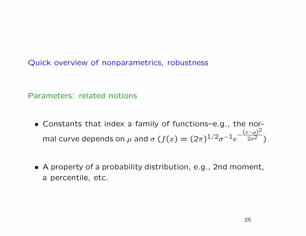
Quick overview of nonparametrics, robustness
Parameters: related notions
• Constants that index a family of functions–e.g., the nor-
mal curve depends on µ and σ (f(x) = (2π)1/2σ−1e−(x−µ)2
2σ2 )
• A property of a probability distribution, e.g., 2nd moment,
a percentile, etc.
25

Parametric statistics: assume a functional form for the prob-ability distribution of the observations; worry perhaps aboutsome parameters in that function.
Non-parametric statistics: fewer, weaker assumptions aboutthe probability distribution. E.g., randomization model, orobservations are iid.
Density estimation, nonparametric regression: Infinitely manyparameters. Requires regularity assumptions to make infer-ences. Plus iid or something like it.
Semiparametrics: Underlying functional form unknown, butrelationship between different groups is parametric. E.g., Coxproportional hazards model.
Robust statistics: assume a functional form for the proba-bility distribution, but worry about whether the procedure issensitive to “small” departures from that assumed form.
26

Groups A group is an ordered pair (G,×), where G is a col-lection of objects (the elements of the group) and × is amapping from G
⊗G onto G,
× : G⊗G → G
(a, b) 7→ a× b,
satisfying the following axioms:
1. ∃e ∈ G s.t. ∀a ∈ G, e× a = a. The element e is called theidentity .
2. For each a ∈ G, ∃a−1 ∈ G s.t. a−1×a = e. (Every elementhas an inverse.)
3. If a, b, c ∈ G, then a × (b × c) = (a × b) × c. (The groupoperation is associative.)
27
Abelian groups If, in addition, for every a, b ∈ G, a× b = b× a(if the group operation commutes), we say that (G,×) is an
Abelian group or commutative group.
28
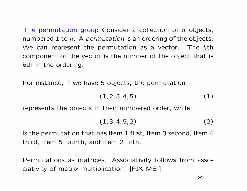
The permutation group Consider a collection of n objects,
numbered 1 to n. A permutation is an ordering of the objects.
We can represent the permutation as a vector. The kth
component of the vector is the number of the object that is
kth in the ordering.
For instance, if we have 5 objects, the permutation
(1,2,3,4,5) (1)
represents the objects in their numbered order, while
(1,3,4,5,2) (2)
is the permutation that has item 1 first, item 3 second, item 4
third, item 5 fourth, and item 2 fifth.
Permutations as matrices. Associativity follows from asso-
ciativity of matrix multiplication. [FIX ME!]
29
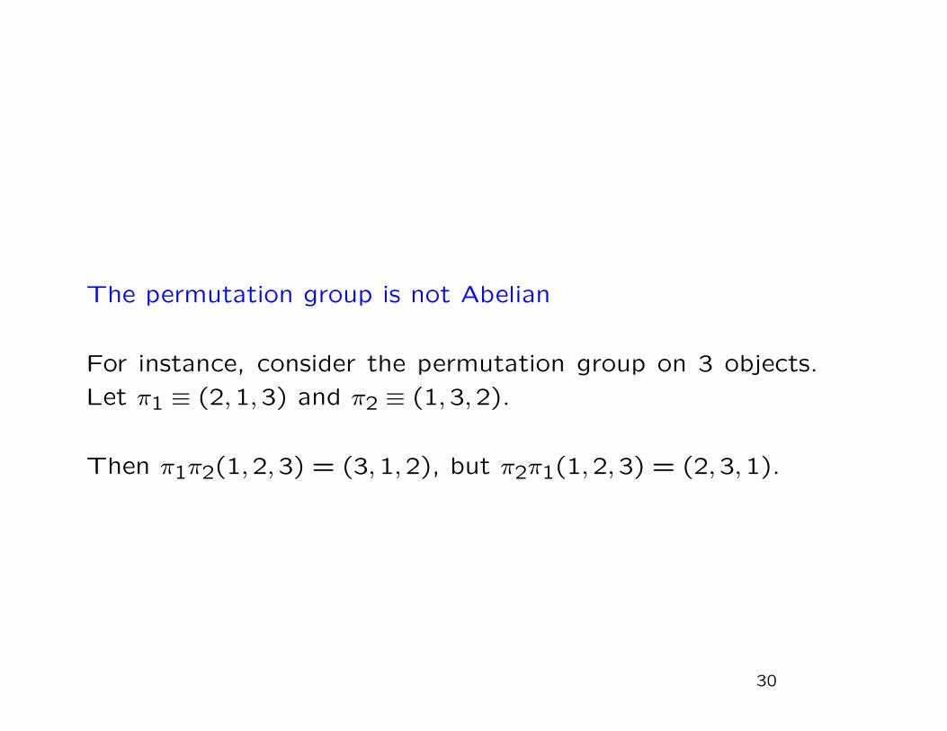
The permutation group is not Abelian
For instance, consider the permutation group on 3 objects.
Let π1 ≡ (2,1,3) and π2 ≡ (1,3,2).
Then π1π2(1,2,3) = (3,1,2), but π2π1(1,2,3) = (2,3,1).
30
Simulation: pseudo-random number generation
Most computers cannot generate truly random numbers, al-
though there is special equipment that can (usually, these rely
on a physical source of “noise,” such as a resistor or a radia-
tion detector). Most so-called random numbers generated by
computers are really “pseudo-random” numbers, sequences
generated by a software algorithm called a pseudo-random
number generator (PRNG) from a starting point, called a
seed. Pseudo-random numbers behave much like random
numbers for many purposes.
The seed of a pseudo-random number generator can be thought
of as the initial state of the algorithm. Each time the algo-
rithm produces a number, it alters its state—deterministically.
If you start a given algorithm from the same seed, you will
get the same sequence of pseudo-random numbers.31

Each pseudo-random number generator has only finitely many
states. Eventually—after the period of the generator, the
generator gets back to its initial state and the sequence re-
peats. If the state of the PRNG is n bits long, the period
of the PRNG is at most 2n bits—but can be substantially
shorter, depending on the algorithm.
Better generators have more states and longer periods, but
that comes at a price: speed. There is a tradeoff between the
computational efficiency of a pseudo-random number gener-
ator and the difficulty of telling that its output is not really
random (measured, for example, by the number of bits one
must examine).
32
Evaluating PRNGs
See http://csrc.nist.gov/rng/ for a suite of tests of pseudo-
random number generators. Tests can be based on statistics
such as the number of zero and one bits in a block or se-
quence, the number of runs in sequences of differing lengths,
the length of the longest run, spectral properties, compress-
ibility (the less random a sequence is, the easier it is to com-
press), and so on.
33

You should check which PRNG is used by any software pack-age you rely on for simulations. Linear Congruential Gener-ators are of the form
xi = ((axi−1 + b) mod m)/(m− 1).
They used to be popular but are best avoided. (They tendto have a short period, and the sequences have underlyingregularity that can spoil performance for many purposes. Forinstance, if the LCG is used to generate n-dimensional points,those points lie on at most m1/n hyperplanes in IRn.
For statistical simulations, a particularly good, efficient pseudo-random number generator is the Mersenne Twister. Thestate of the Mersenne Twister is a 624-vector of 32-bit inte-gers and a pointer to one of those vectors. It has a periodof 219937 − 1, which is on the order of 106001. It is imple-mented in R (it’s the default), Python, Perl, and many otherlanguages. For cryptography, a higher level of randomness isneeded than for most statistical simulations.
34

No pseudo-random number generator is best for all purposes.
But some are truly terrible.
For instance, the PRNG in Microsoft Excel is a faulty im-
plementation of an algorithm (the Wichmann-Hill algorithm,
which combines four LCGs) that isn’t good in the first place.
35
McCullough, B.D., Heiser, David A., 2008. On the accuracy
of statistical procedures in Microsoft Excel 2007. Computa-
tional Statistics and Data Analysis 52 (10), 4570–4578.
http://www.sciencedirect.com/science?_ob=MImg&_imagekey=B6V8V-4S1S6FC-5-3F&_
cdi=5880&_user=4420&_orig=mlkt&_coverDate=06%2F15%2F2008&_sk=
999479989&view=c&wchp=dGLbVzb-zSkWb&md5=85d93a6c0700f2dbc483f5ed6b239db2&ie=
/sdarticle.pdf
Excerpt: Excel 2007, like its predecessors, fails a standard set
of intermediate-level accuracy tests in three areas: statisti-
cal distributions, random number generation, and estimation.
Additional errors in specific Excel procedures are discussed.
Microsoft’s continuing inability to correctly fix errors is dis-
cussed. No statistical procedure in Excel should be used until
Microsoft documents that the procedure is correct; it is not
safe to assume that Microsoft Excel’s statistical procedures36

give the correct answer. Persons who wish to conduct sta-
tistical analyses should use some other package.
If users could set the seeds, it would be an easy matter to
compute successive values of the WH RNG and thus ascer-
tain whether Excel is correctly generating WH RNGs. We
pointedly note that Microsoft programmers obviously have
the ability to set the seeds and to verify the output from the
RNG; for some reason they did not do so. Given Microsoft’s
previous failure to implement correctly the WH RNG, that
the Microsoft programmers did not take this easy and obvi-
ous opportunity to check their code for the patch is absolutely
astounding.

McCullough, B.D., 2008. Microsoft’s ‘Not the Wichmann-
Hill’ random number generator. Computational Statistics and
Data Analysis 52 (10), 4587–4593.
http://www.sciencedirect.com/science?_ob=MImg&_imagekey=B6V8V-4S21TGC-2-22&_
cdi=5880&_user=4420&_orig=search&_coverDate=06%2F15%2F2008&_
sk=999479989&view=c&wchp=dGLbVtz-zSkzk&md5=38238ccd25a60a408480df345be88e34&ie=
/sdarticle.pdf
37
Drawing (pseudo-)random samples using PRNGs
A standard technique for drawing a pseudo-random sample of
size n from N item is to assign each of the N items a pseudo-
random number, then take the sample to be the n items that
were assigned the n smallest pseudo-random numbers.
Note that when N is large and n is a moderate fraction of
N , PRNGs might not be able to generate all(Nn
)subsets.
Henceforth, will assume that the PRNG is “good enough”
that its departure from randomness does not affect the ac-
curacy our simulations enough to matter.
38
Bernoulli trials
A Bernoulli trial is a random experiment with two possible
outcomes, success and failure. The probability of success is
p; the probability of failure is 1− p.
Events A and B are independent if P (AB) = P (A)P (B).
A collection of events is independent if the probability of the
intersection of every subcollection is equal to the product of
the probabilities of the members of that subcollection.
Two random variables are independent if every event deter-
mined by the first random variable is independent of every
event determined by the second.
39

Binomial distribution
Consider a sequence of n independent Bernoulli trials with
the same probability p of success in each trial. Let X be the
total number of successes in the n trials.
Then X has a binomial probability distribution:
Pr(X = x) =(nx
)px(1− p)n−x. (3)
40
Hypergeometric distribution
A simple random sample of size n from a finite population of
N things is a random sample drawn without replacement in
such a way that each of the(Nn
)subsets of size n from the
population is equally likely to be the sample.
Consider drawing a simple random sample from a population
of N objects of which G are good and N −G are bad. Let X
be the number of good objects in the sample.
Then X has a hypergeometric distribution:
P (X = x) =
(Gx
)(N−Gn−x
)(Nn
) , (4)
for max(0, n− (N −G)) ≤ x ≤ min(n,G).
41
Hypothesis testing
Much of this course concerns hypothesis tests. We will think
of a test as consisting of a set of possible outcomes (data),
called the acceptance region. The complement of the accep-
tance region is the rejection region.
We reject the null hypothesis if the data are in the rejection
region.
The significance level α is an upper bound on the chance
that the outcome will turn out to be in the rejection region
if the null hypothesis is true.
42

Conditional tests
The chance is sometimes a conditional probability rather than
an unconditional probability. That is, we have a rule that
generates an acceptance region that depends on some aspect
of the data. We’ve already seen an example of that in the
rat cortical mass experiment. There, we conditioned on the
cortical masses, but not on the the randomization.
If we test to obtain conditional significance level α (or smaller)
no matter what the data are, then the unconditional signifi-
cance level is still α:
PrType I error =∫x
PrType I error|X = xµ(dx)
≤ supx
PrType I error|X = x.
43

P -values
Suppose we have a family of hypothesis tests for testing a
given null hypothesis at every significance level α ∈ (0,1).
Let Aα denote the acceptance region for the test at level α.
Suppose further that the tests nest, in the sense that if α1 <
α2, then Aα1 ⊂ Aα2
Then the P -value of the hypothesis (for data X) is
infα : X /∈ Aα (5)
44

Confidence sets
We have a collection of hypotheses H. We know that some
H ∈ H must be true—but we don’t know which one.
A rule that uses the data to select a subset of H is a 1 − αconfidence procedure if the chance that it selects a subset
that includes H is at least 1− α.
The subset that the rule selects is called a 1− α confidence
set.
The coverage probability at G is the chance that the rule
selects a set that includes G if G ∈ H is the true hypothesis.
45
Duality between tests and confidence sets
Suppose that some hypothesis H ∈ H must be true. Suppose
we have a family of significance-level α tests AG : G ∈ Hsuch that for each G ∈ H,
PrGX /∈ AG ≤ α. (6)
Then the set
C(X) ≡ G ∈ H : AG 3 X (7)
is a 1− α confidence set for the true H.
46

Tests and confidence sets for Bernoulli p
We have Xj ∼ Bernoulli(p). Can draw as big an iid sample
Xjnj=1 as we like.
We want to test the hypothesis that p ≤ p0 at level α and we
want to find a 1-sided upper confidence interval for p.
Or might want 2-sided confidence interval, or to test the
hypothesis p > p0, or a 1-sided lower confidence interval.
47
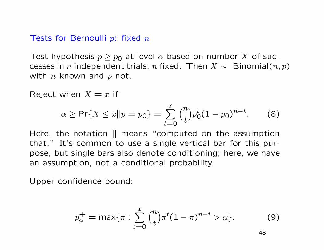
Tests for Bernoulli p: fixed n
Test hypothesis p ≥ p0 at level α based on number X of suc-cesses in n independent trials, n fixed. Then X ∼ Binomial(n, p)with n known and p not.
Reject when X = x if
α ≥ PrX ≤ x||p = p0 =x∑t=0
(nt
)pt0(1− p0)n−t. (8)
Here, the notation || means “computed on the assumptionthat.” It’s common to use a single vertical bar for this pur-pose, but single bars also denote conditioning; here, we havean assumption, not a conditional probability.
Upper confidence bound:
p+α = maxπ :
x∑t=0
(nt
)πt(1− π)n−t > α. (9)
48

Upper confidence bound for binomial p
binoUpperCL <- function(n, x, cl = 0.975, inc=0.000001, p=x/n)
if (x < n)
f <- pbinom(x, n, p, lower.tail = TRUE);
while (f >= 1-cl)
p <- p + inc;
f <- pbinom(x, n, p, lower.tail = TRUE)
p
else
1.0
49
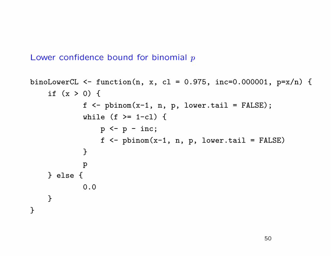
Lower confidence bound for binomial p
binoLowerCL <- function(n, x, cl = 0.975, inc=0.000001, p=x/n)
if (x > 0)
f <- pbinom(x-1, n, p, lower.tail = FALSE);
while (f >= 1-cl)
p <- p - inc;
f <- pbinom(x-1, n, p, lower.tail = FALSE)
p
else
0.0
50
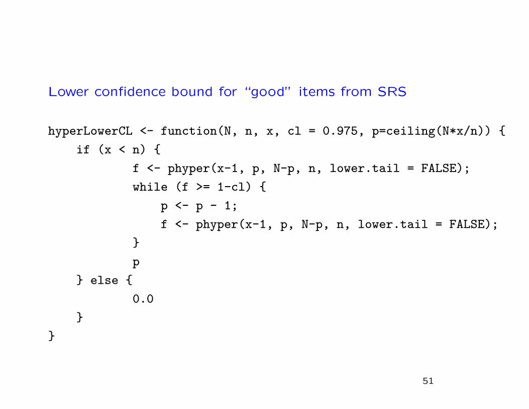
Lower confidence bound for “good” items from SRS
hyperLowerCL <- function(N, n, x, cl = 0.975, p=ceiling(N*x/n))
if (x < n)
f <- phyper(x-1, p, N-p, n, lower.tail = FALSE);
while (f >= 1-cl)
p <- p - 1;
f <- phyper(x-1, p, N-p, n, lower.tail = FALSE);
p
else
0.0
51

Upper confidence bound for “good” items from SRS
hyperUpperCL <- function(N, n, x, cl = 0.975, p=floor(N*x/n))
if (x < n)
f <- phyper(x, p, N-p, n, lower.tail = TRUE);
while (f >= 1-cl)
p <- p + 1;
f <- phyper(x, p, N-p, n, lower.tail = TRUE);
p
else
1.0
52
Sequential test for p
If generating each Xj is expensive (e.g., if it involves running a
climate model on supercomputer clusters for months), might
want to minimize the sample size. Sequential testing: draw
until you have strong evidence that p ≤ p0 (or that p > p0).
Null: p > p0. Control the chance of type I error.
Two common criteria: expected sample size at fixed p and
maximum expected sample size.
α: maximum chance of rejecting null when p > p0.
β: maximum chance of not rejecting null when p ≤ p1 < p0.
53
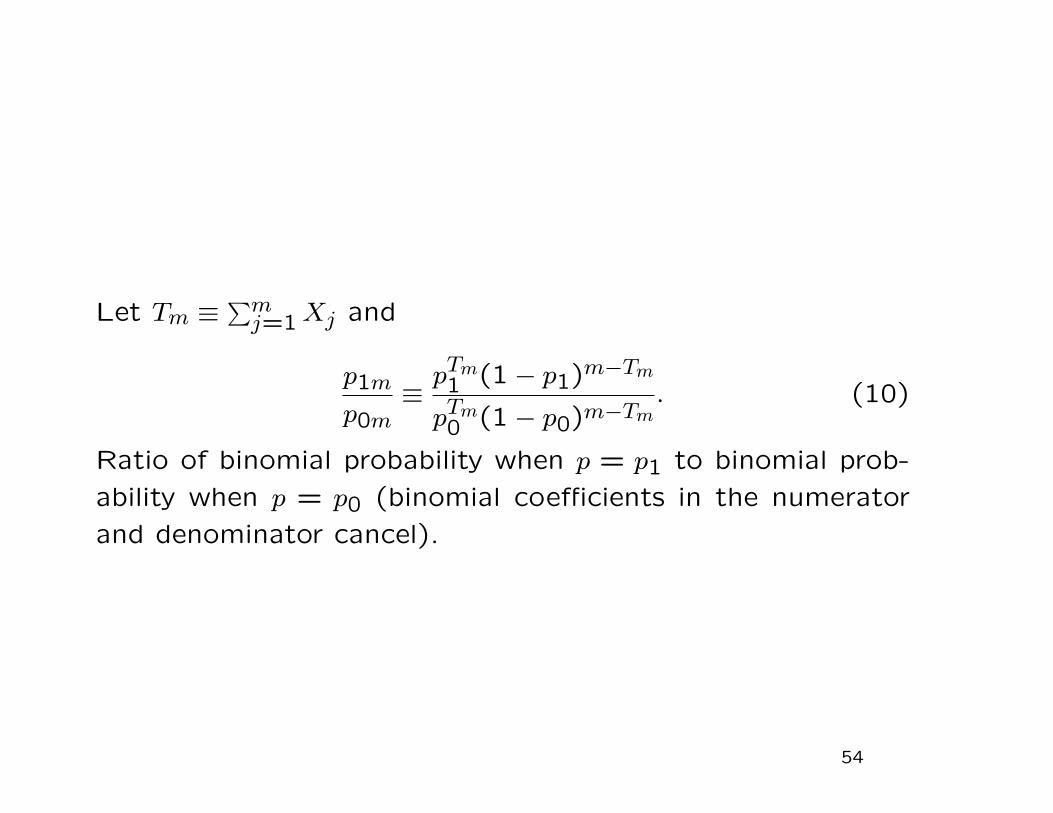
Let Tm ≡∑mj=1Xj and
p1m
p0m≡pTm1 (1− p1)m−Tm
pTm0 (1− p0)m−Tm. (10)
Ratio of binomial probability when p = p1 to binomial prob-
ability when p = p0 (binomial coefficients in the numerator
and denominator cancel).
54
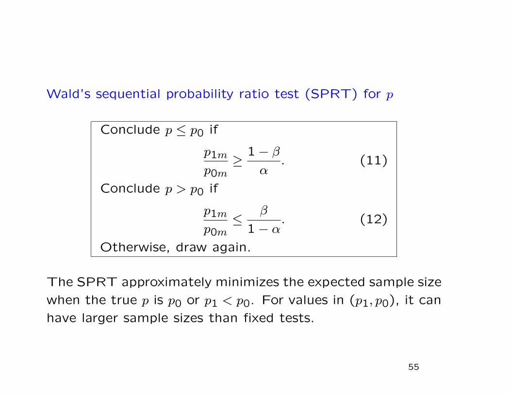
Wald’s sequential probability ratio test (SPRT) for p
Conclude p ≤ p0 if
p1m
p0m≥
1− βα
. (11)
Conclude p > p0 if
p1m
p0m≤
β
1− α. (12)
Otherwise, draw again.
The SPRT approximately minimizes the expected sample size
when the true p is p0 or p1 < p0. For values in (p1, p0), it can
have larger sample sizes than fixed tests.
55
SPRT miracle
Don’t need to know the distribution of the test statistic under
the null hypothesis to find the critical values for the test.
56
Derivation of Wald’s SPRT
Testing between two hypotheses, H0 and H1, on the basis
of data Xj ⊂ X , with X a measurable space. According to
both hypotheses, the Xj are iid. Each hypothesis specifies
a probability distribution for the data.
Suppose those two distributions are absolutely continuous
with respect to some dominating measure µ on X . Let f0 be
the density (wrt µ) of the distribution of Xj if H0 is true and
let f1 be the density (wrt µ) of the distribution of Xj if H1
is true.
57
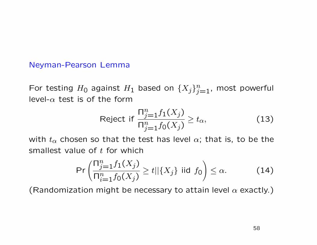
Neyman-Pearson Lemma
For testing H0 against H1 based on Xjnj=1, most powerful
level-α test is of the form
Reject ifΠnj=1f1(Xj)
Πnj=1f0(Xj)
≥ tα, (13)
with tα chosen so that the test has level α; that is, to be the
smallest value of t for which
Pr
(Πnj=1f1(Xj)
Πni=1f0(Xj)
≥ t||Xj iid f0
)≤ α. (14)
(Randomization might be necessary to attain level α exactly.)
58

Derivation of SPRT (contd)
At stage m, divide outcome space into 3 disjoint regions,
A0m, A1m and Am.
Draw X1. If X1 ∈ A01, accept H0 and stop. If X1 ∈ A11,
accept H1 and stop. If X1 ∈ A1, draw X2.
If you draw Xm, then: If Xm ∈ A0m, accept H0 and stop. If
Xm ∈ A1m, accept H1 and stop. If Xm ∈ Am, draw Xm+1.
59

Derivation (contd)
A fixed-n test is a special case: A0m and A1m are empty for
m < n (so Am is the entire outcome space when m < n).
A0n is the acceptance region of the test, and A1n is the
complement of A0n (so Am is empty when m = n).
60

Derivation (contd)
Suppose sequential procedure stops after drawing XN . N is
random.
Suppose S is a particular sequential test procedure. Let
IE(N ||h) = IE(N ||h, S) be the expected value of N if Hh is
true, h ∈ 0,1, for test S.
Tests S and S′ have the same strength if they have the same
chances of type I errors and of type II errors (α and β).
If S and S′ have the same strength, S is better than S′ if
IE(N ||h, S) ≤ IE(N ||h, S′) for h = 1,2, with strict inequality for
either h = 1 or h = 2 (or both).
61
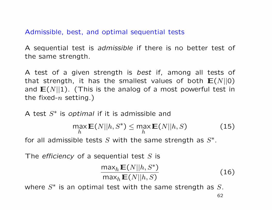
Admissible, best, and optimal sequential tests
A sequential test is admissible if there is no better test ofthe same strength.
A test of a given strength is best if, among all tests ofthat strength, it has the smallest values of both IE(N ||0)and IE(N ||1). (This is the analog of a most powerful test inthe fixed-n setting.)
A test S∗ is optimal if it is admissible and
maxh
IE(N ||h, S∗) ≤ maxh
IE(N ||h, S) (15)
for all admissible tests S with the same strength as S∗.
The efficiency of a sequential test S is
maxh IE(N ||h, S∗)maxh IE(N ||h, S)
(16)
where S∗ is an optimal test with the same strength as S.62
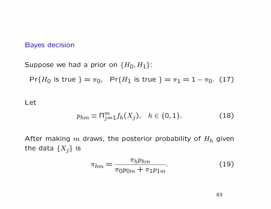
Bayes decision
Suppose we had a prior on H0, H1:
PrH0 is true = π0, PrH1 is true = π1 = 1− π0. (17)
Let
phm ≡ Πmj=1fh(Xj), h ∈ 0,1. (18)
After making m draws, the posterior probability of Hh given
the data Xj is
πhm =πhphm
π0p0m + π1p1m. (19)
63
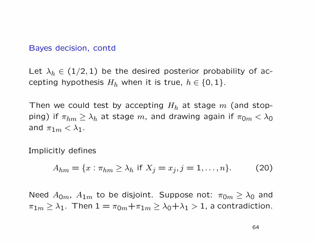
Bayes decision, contd
Let λh ∈ (1/2,1) be the desired posterior probability of ac-
cepting hypothesis Hh when it is true, h ∈ 0,1.
Then we could test by accepting Hh at stage m (and stop-
ping) if πhm ≥ λh at stage m, and drawing again if π0m < λ0
and π1m < λ1.
Implicitly defines
Ahm = x : πhm ≥ λh if Xj = xj, j = 1, . . . , n. (20)
Need A0m, A1m to be disjoint. Suppose not: π0m ≥ λ0 and
π1m ≥ λ1. Then 1 = π0m+π1m ≥ λ0+λ1 > 1, a contradiction.
64
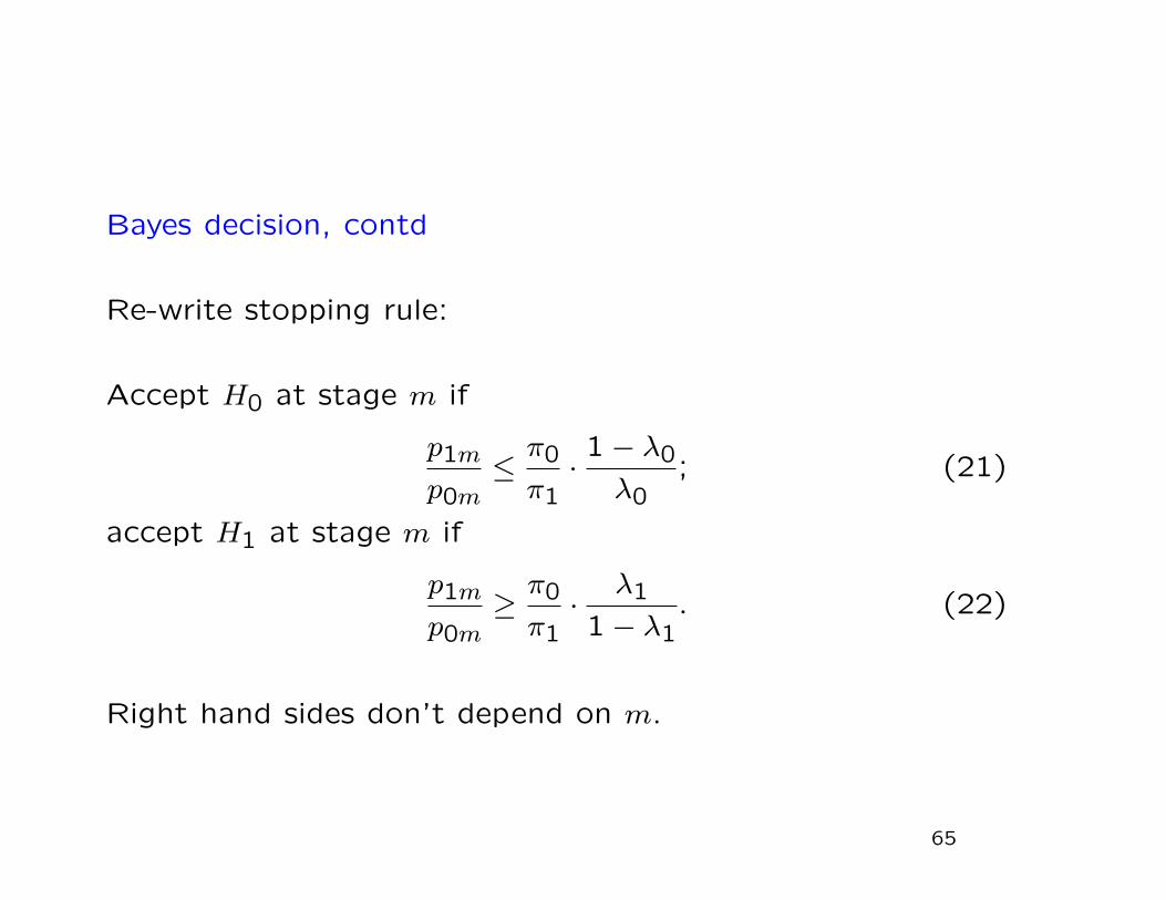
Bayes decision, contd
Re-write stopping rule:
Accept H0 at stage m if
p1m
p0m≤π0
π1·
1− λ0
λ0; (21)
accept H1 at stage m if
p1m
p0m≥π0
π1·
λ1
1− λ1. (22)
Right hand sides don’t depend on m.
65
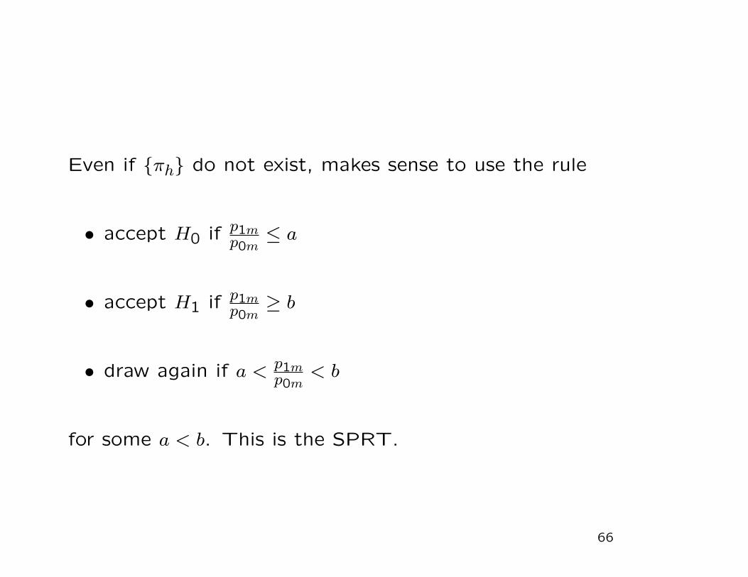
Even if πh do not exist, makes sense to use the rule
• accept H0 if p1mp0m≤ a
• accept H1 if p1mp0m≥ b
• draw again if a < p1mp0m
< b
for some a < b. This is the SPRT.
66
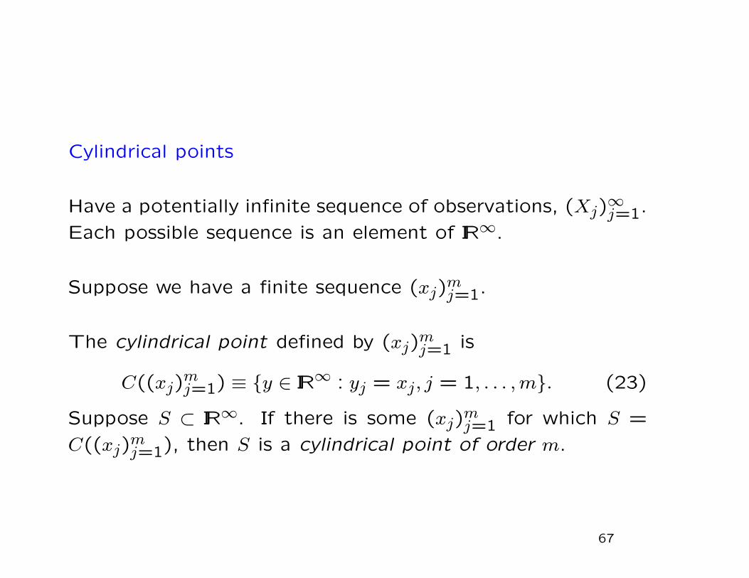
Cylindrical points
Have a potentially infinite sequence of observations, (Xj)∞j=1.
Each possible sequence is an element of IR∞.
Suppose we have a finite sequence (xj)mj=1.
The cylindrical point defined by (xj)mj=1 is
C((xj)mj=1) ≡ y ∈ IR∞ : yj = xj, j = 1, . . . ,m. (23)
Suppose S ⊂ IR∞. If there is some (xj)mj=1 for which S =
C((xj)mj=1), then S is a cylindrical point of order m.
67
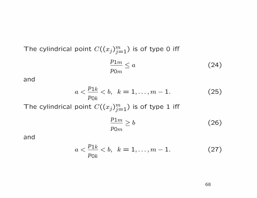
The cylindrical point C((xj)mj=1) is of type 0 iff
p1m
p0m≤ a (24)
and
a <p1k
p0k< b, k = 1, . . . ,m− 1. (25)
The cylindrical point C((xj)mj=1) is of type 1 iff
p1m
p0m≥ b (26)
and
a <p1k
p0k< b, k = 1, . . . ,m− 1. (27)
68
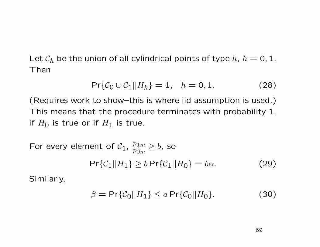
Let Ch be the union of all cylindrical points of type h, h = 0,1.
Then
PrC0 ∪ C1||Hh = 1, h = 0,1. (28)
(Requires work to show–this is where iid assumption is used.)
This means that the procedure terminates with probability 1,
if H0 is true or if H1 is true.
For every element of C1, p1mp0m≥ b, so
PrC1||H1 ≥ bPrC1||H0 = bα. (29)
Similarly,
β = PrC0||H1 ≤ aPrC0||H0. (30)
69
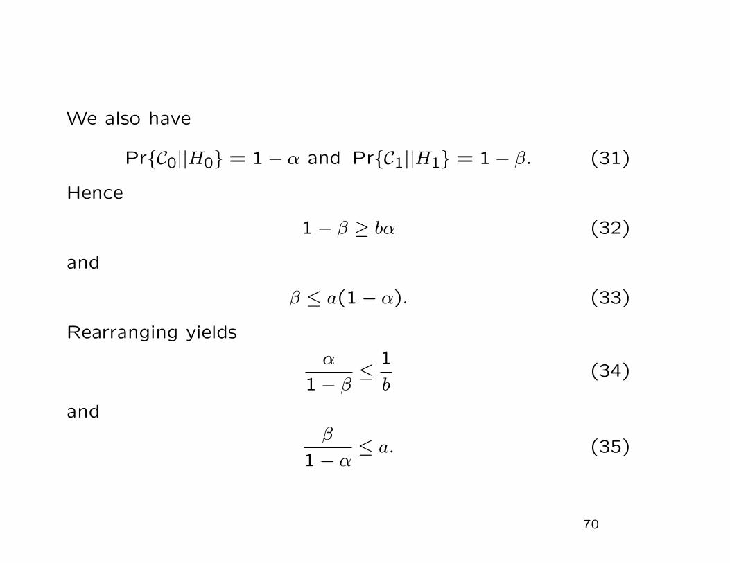
We also have
PrC0||H0 = 1− α and PrC1||H1 = 1− β. (31)
Hence
1− β ≥ bα (32)
and
β ≤ a(1− α). (33)
Rearranging yields
α
1− β≤
1
b(34)
andβ
1− α≤ a. (35)
70
Notes:
• iid assumption can be weakened substantially. Only used
to prove that PrC0 ∪ C1||Hh = 1.
• only need to know the likelihood function under the two
hypotheses, α, and β
• can sharpen the choice of thresholds, but not by much if
α and β are small.
71

References on sequential tests for Bernoulli p
[?, ?, ?]
References on sequential tests forMonte Carlo p
[?, ?, ?]
References on 2-SPRT, etc. [FIX ME!]
72

Assignment: comparing SPRT and fixed sample-size tests
Implement the SPRT in R from scratch.
Taking p0 = 0.05, p1 = 0.045, α = 0.001, β = 0.01, estimate
(by simulation) the expected number of samples that must
be drawn when p = 0.01,0.02, . . . ,0.1.
Compare the expected sample sizes with sample sizes for a
fixed-n test with the same α and β.
Justify your choice of the number of replications to use in
your simulations.
For each of the 10 scenarios, report the empirical fraction of
type I and type II errors and 99% confidence intervals for the
probabilities of those errors.73
Assignment hint
Order of operations matters for accuracy and stability.
Raising a small number to a high power will eventually give
you zero (to machine precision). If you calculate the nu-
merator and the denominator in SPRT separately, you will
eventually get nonsense as m gets large.
Rather than take a ratio of large products that are each going
to zero, it’s much more stable to take a product of ratios that
are all close to 1.
74

Assignment hint, contd.
So, compute
(p1/p0)Tm((1− p1)/(1− p0))m−Tm (36)
rather than
[pTm1 (1− p1)m−Tm]/[pTm0 (1− p0)m−Tm]. (37)
If you want to work with the log SPR, compute
Tm log((p1/p0) + (m− Tm) log((1− p1)/(1− p0)) (38)
rather than
Tm log p1+(m−Tm) log(1−p1)−Tm log(p0)−(m−Tm) log(1−p0).
(39)
75

Fisher’s exact test, Fisher’s “Lady Tasting Tea” experiment
Under what groups is the distribution of the the data invariant
in those problems?
http://statistics.berkeley.edu/~stark/SticiGui/Text/percentageTests.
htm#fisher_dependent
http://statistics.berkeley.edu/~stark/Teach/S240/Notes/ch3.
htm
76

General test based on group invariance
Follow Romano (1990).
Data X ∼ P takes values in X .
G is a finite group of transformations from X to X . #G = G.
Want to test null hypothesis H0 : P ∈ Ω0.
Suppose H0 implies that P is invariant under G:
∀g ∈ G, X ∼ gX. (40)
The orbit of x (under G) is gx : g ∈ G. (Does the orbit of x
always contain G points?)
77
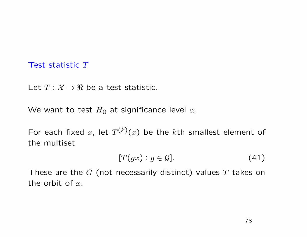
Test statistic T
Let T : X → < be a test statistic.
We want to test H0 at significance level α.
For each fixed x, let T (k)(x) be the kth smallest element of
the multiset
[T (gx) : g ∈ G]. (41)
These are the G (not necessarily distinct) values T takes on
the orbit of x.
78
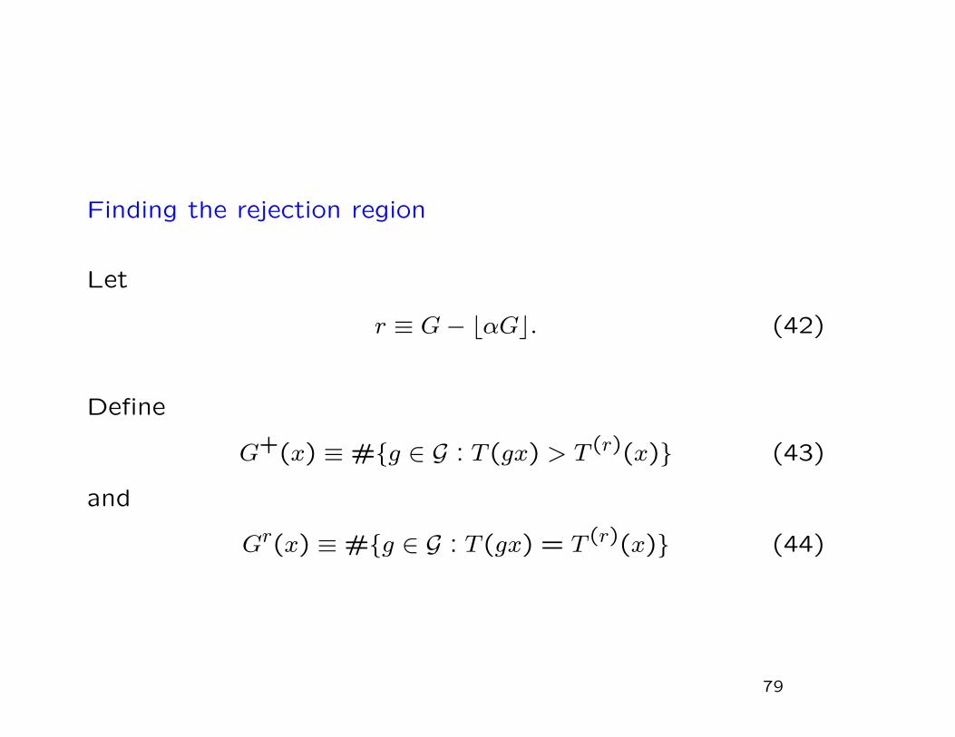
Finding the rejection region
Let
r ≡ G− bαGc. (42)
Define
G+(x) ≡#g ∈ G : T (gx) > T (r)(x) (43)
and
Gr(x) ≡#g ∈ G : T (gx) = T (r)(x) (44)
79
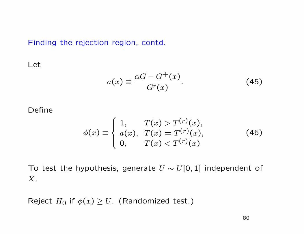
Finding the rejection region, contd.
Let
a(x) ≡αG−G+(x)
Gr(x). (45)
Define
φ(x) ≡
1, T (x) > T (r)(x),
a(x), T (x) = T (r)(x),
0, T (x) < T (r)(x)
(46)
To test the hypothesis, generate U ∼ U [0,1] independent of
X.
Reject H0 if φ(x) ≥ U . (Randomized test.)
80

Test has level α unconditionally
For each x ∈ X ,∑g∈G
φ(gx) = G+(x) + a(x)Gr(x) = αG. (47)
So if X ∼ gX ∼ P for all g ∈ G,
α = IEP1
G
∑g∈G
φ(gX)
=1
G
∑g∈G
IEPφ(X)
= IEPφ(X). (48)
The unconditional chance of a Type I error is exactly α.
81
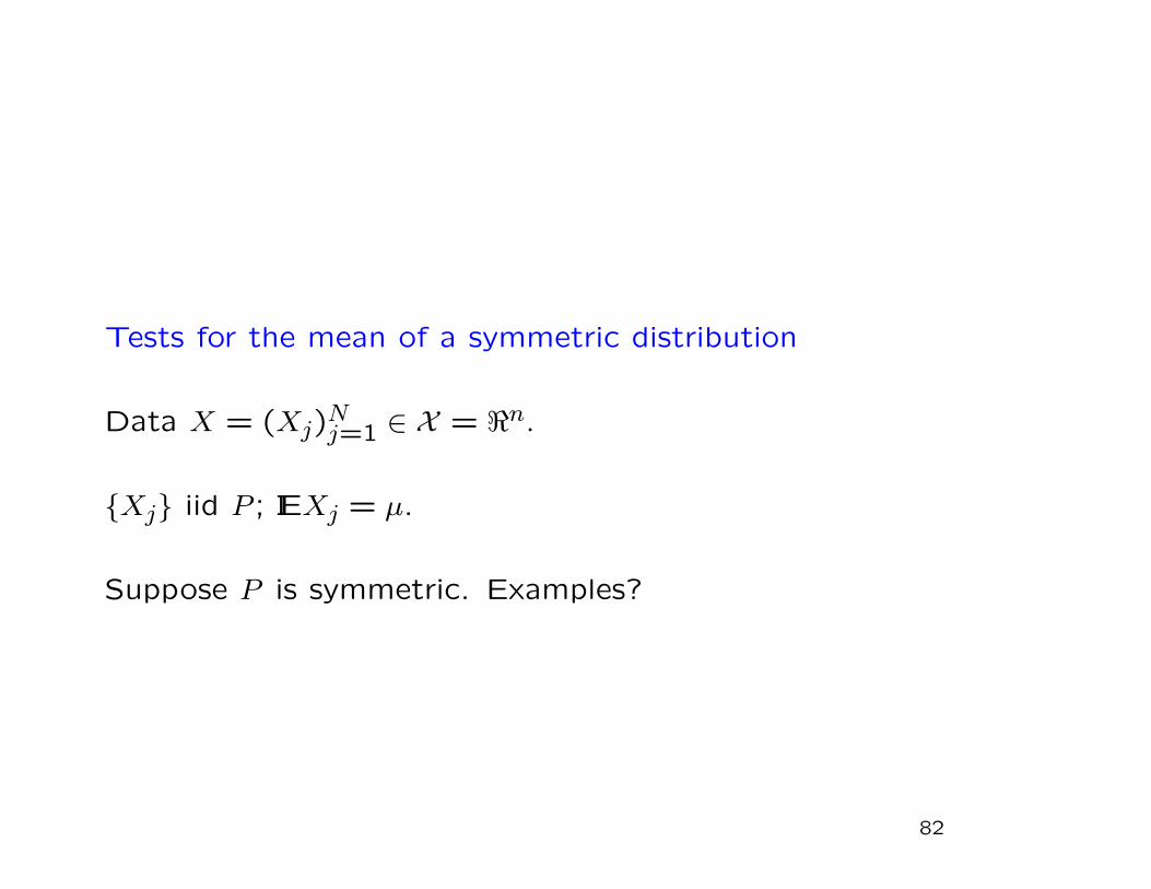
Tests for the mean of a symmetric distribution
Data X = (Xj)Nj=1 ∈ X = <n.
Xj iid P ; IEXj = µ.
Suppose P is symmetric. Examples?
82

Reflection group
Let Gµ be the group of reflections of coordinates about µ.
Let x ∈ <n. Each g ∈ Gµ is of the form
g(x) = (µ+ (−1)γj(xj − µ))nj=1 (49)
for some γ = (γj)nj=1 ∈ 0,1
n.
Is Gµ really a group?
What’s the identity element? What’s the inverse of g? What
γ corresponds to g1g2?
What is G, the number of elements of Gµ?
83

What is the orbit of a point x under Gµ? Are there always 2n
distinct elements of the orbit?
Test statistic
T (X) = |X − µ0| =
∣∣∣∣∣∣1nn∑
j=1
Xj − µ0
∣∣∣∣∣∣ . (50)
If IEXj = µ0, this is expected to be small—but how large a
value would be surprising?
84
If the expected value of Xj is µ and P is symmetric (i.e., if
H0 is true), the 2n potential data
gX : g ∈ Gµ (51)
in the orbit of X under G are equally likely.
Hence, the values in the multiset
[T (gx) : g ∈ Gµ] (52)
are equally likely, conditional on the event that X is in the
orbit of x.
85
How to test H0: µ = µ0?
We observe X = x.
If fewer than αG values in [T (gx) : g ∈ Gµ0] are greater than
or equal to T (x), reject. If more than αG values are greater
than T (x), don’t reject. Otherwise, randomize.
86
If n is big . . .
How can we sample at random from the orbit?
Toss fair coin n times in sequence, independently. Take γj =
1 if the jth toss gives heads; γj = 0 if tails.
Amounts to sampling with replacement from the orbit of x.
87
Other test statistics?
Could use t-statistic, but calibrate critical value using the
permutation distribution.
Could use a measure of dispersion around the hypothesized
mean (the true mean minimizes expected RMS difference,
assuming variance is finite).
What about counting the number of values that are above
µ0?
Define
T (x) ≡n∑
j=1
1x≥µ0. (53)
88

Sign test for the median
We are assuming P is symmetric, so the expected value andmedian are equal.
To avoid unhelpful complexity, suppose P is continuous. Then
PrXj ≥ µ = 1/2, (54)
1Xj≥µnj=1 are iid Bernoulli(1/2), (55)
and
T (X) ∼ Binomial(n,1/2). (56)
This leads to the sign test: Reject the hypothesis that themedian is µ0 if T (X) is too large or too small. Thresh-olds set to get level α test, using the fact that T (X) ∼Binomial(n,1/2).
89

Is the sign test equivalent to the permutation test for the
same test statistic?
Suppose we are using the test statistic T (x) =∑nj=1 1x≥µ0
.
Do the permutation test and the sign test reject for the same
values of x ∈ X?
Suppose no component of x is equal to µ0. According to the
sign test, the chance that T (x) = k is(nk
)2−n if the null is
true.
What’s the chance that T (x) = k according to the permuta-
tion test? There are G = 2n points in the orbit of x under
G. If the null is true, all have equal probability 2−n. Of
these points,(nk
)have k components with positive deviations
from µ0. Hence, for the permutation test, the chance that
T (x) = k is also(nk
)2−n: The two tests are equivalent.
90
Confidence intervals for µ for symmetric P
Invert two-sided tests.
91
What if P is not symmetric?
Romano [?]: the permutation test based on either the sample
mean or Studentized sample mean still have the right level
asymptotically.
Heuristic: if VarXj is finite and n is large, the sample mean
is approximately normal—and thus symmetric—even when
the distribution of Xj is not symmetric. The permutation
distribution of the sample mean or Studentized sample mean
under the null approaches a normal with mean zero and the
“right” variance.
92
Assignment
Implement the two-sided, one-sample permutation test using
the sample mean as the test statistic, simulate results with
and without symmetry.
Compare the power with the t-test for a normal.
Compare power and level under symmetry with P not normal.
Compare power and level when P is asymmetric (e.g., abso-
lute value of a Normal, non-central χ2 with a small number
of degrees of freedom, triangular distribution, . . . )
93

Runs test for independence
Suppose we toss a biased coin N times, independently. The
coin has chance p of landing heads in each toss and chance
1− p of landing tails in each toss. We do not know p.
Since the tosses are iid, they are exchangeable: The chance
of any particular sequence of n heads and N − n tails is
pn(1 − p)N−n. The probability distribution is invariant un-
der permutations of the trials.
For any particular observed sequence of n heads and N − ntails, the orbit of the data under the action of the permu-
tation group consists of all(Nn
)sequences of n heads (H)
and N − n tails (T). That amounts to conditioning on the
number n of heads in the (fixed) number N of tosses, but
not on whether each toss resulted in H or T.94
Runs test, contd.
A run is a sequence of H or T. The sequence HHTHTTTHTHhas 7 runs: HH, T, H, TTT, H, T and H. If the tosses areindependent, each arrangement of the n heads and m ≡ N−ntails among the N tosses has probability 1/
(Nn
); there are
1/(Nn
)equally likely elements in the orbit of the observed
sequence under the permutation group. We will compute the(conditional) probability distribution of R given n, assumingindependence of the trials.
If n = N or if n = 0, R ≡ 1. If k = 1, there are only twopossibilities: first all the heads, then all the tails, or first allthe tails, then all the heads. I.e., the sequence is either
(HH . . . HTT . . . T) or (TT . . . THH . . . H)
The probability that R = 1 is thus 2/(Nn
), if the null hypoth-
esis is true.95
Runs test, contd.
How can R be even, i.e., R = 2k? If the sequence starts withH, we need to choose where to break the sequence of H toinsert T, then where to break that sequence of T to insert H,etc. If the sequence starts with T, we need to choose whereto break the sequence of T to insert H, then where to breakthat sequence of H to insert T, etc.
We need to break the n heads into k groups, which meanspicking k − 1 breakpoints, but the first breakpoint needs tocome after the first H, and the last breakpoint needs to comebefore the nth H, so there are only n − 1 places those k − 1breakpoints can be. And we need to break the m tails intok groups, which means picking k − 1 breakpoints, but thefirst needs to be after the first T and the last needs to bebefore the mth T, so there are only m− 1 places those k− 1breakpoints can be.
96
Runs test, contd.
The number of sequences with R = 2k that start with H is
thus
(n− 1
k − 1
)×(m− 1
k − 1
). (57)
The number of sequences with R = 2k that start with T
is the same (just read right-to-left instead of left-to-right).
Thus, if the tosses are independent and there are n heads in
all,
PR = 2k = 2×(n− 1
k − 1
)×(m− 1
k − 1
)/(Nn
). (58)
97
Runs test, contd.
Now consider how we can have R = 2k+ 1 (odd). Either the
sequence starts and ends with H or it starts and ends with T.
Suppose it starts with H. Then we need to break the string
of n heads in k places to form k + 1 groups using k groups
of tails formed by breaking the m tails in k− 1 places. If the
sequence starts with T, we need to break the m tails in k
places to form k + 1 groups using k groups of heads formed
by breaking the n heads in k − 1 places. Thus, if the tosses
are independent and there are n heads in all,
PR = 2k + 1 =
(n−1k
)×(m−1k−1
)+(n−1k−1
)×(m−1k
)(Nn
) . (59)
98
Runs test, contd.
Nothing in this derivation used the probability p of heads.
The conditional distribution under the null hypothesis de-
pends only on the fact that the tosses are iid, so that all
arrangements with a given number of heads are equally likely.
Note the connection with the sign test for the median and
the one-sample test for the mean of a symmetric istribu-
tion, discussed previously. There, under the null, we had
exchangeability with respect to reflections and permutations.
The alternative still had exchangeability with respect to per-
mutations, but not reflections.
Here, under the null we have exchangeability with respect to
permutations. Under the alternative, we don’t.
99

Runs test, contd.
The runs test is also connected to Fisher’s Exact Test—in
both, we condition on the number of “successes” and look at
whether those successes are distributed in the way we would
expect if the null held.
100
Runs test, contd.
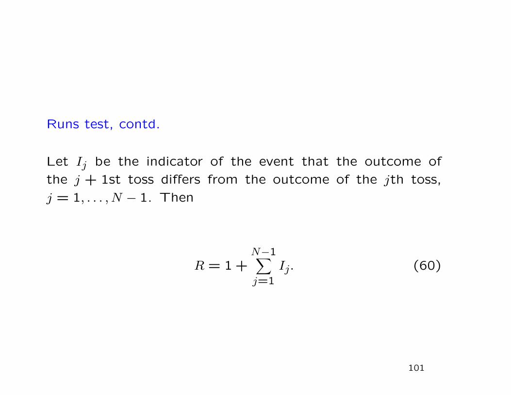
Let Ij be the indicator of the event that the outcome of
the j + 1st toss differs from the outcome of the jth toss,
j = 1, . . . , N − 1. Then
R = 1 +N−1∑j=1
Ij. (60)
101
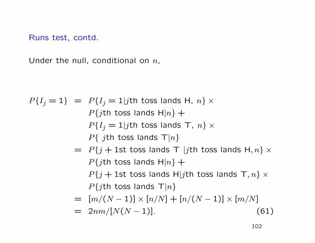
Runs test, contd.
Under the null, conditional on n,
PIj = 1 = PIj = 1|jth toss lands H, n ×Pjth toss lands H|n+
PIj = 1|jth toss lands T, n ×P jth toss lands T|n
= Pj + 1st toss lands T |jth toss lands H, n ×Pjth toss lands H|n+
Pj + 1st toss lands H|jth toss lands T, n ×Pjth toss lands T|n
= [m/(N − 1)]× [n/N ] + [n/(N − 1)]× [m/N ]
= 2nm/[N(N − 1)]. (61)
102
Runs test, contd.
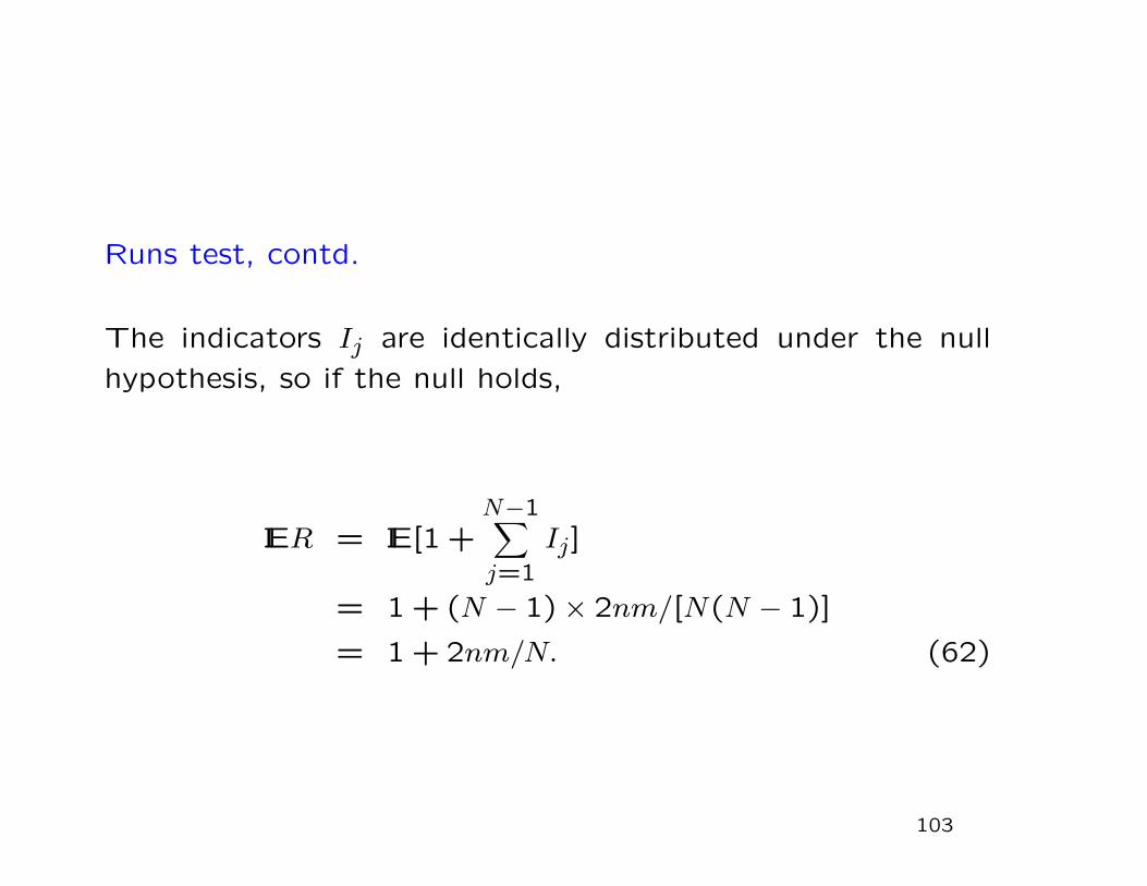
The indicators Ij are identically distributed under the null
hypothesis, so if the null holds,
IER = IE[1 +N−1∑j=1
Ij]
= 1 + (N − 1)× 2nm/[N(N − 1)]
= 1 + 2nm/N. (62)
103
Example of Runs test
Air temperature is measured at noon in a climate-controlled
room for 20 days in a row. We want to test the null hypoth-
esis that temperatures on different days are independent and
identically distributed.
Let Tj be the temperature on day j, j = 1, . . . ,20. If the
measurements were iid, whether each day’s temperature is
above or below a given temperature t is like a toss of a pos-
sibly biased coin, with tosses on different days independent
of each other. We could consider a temperature above t to
be a head and a temperature below t to be a tail.
104
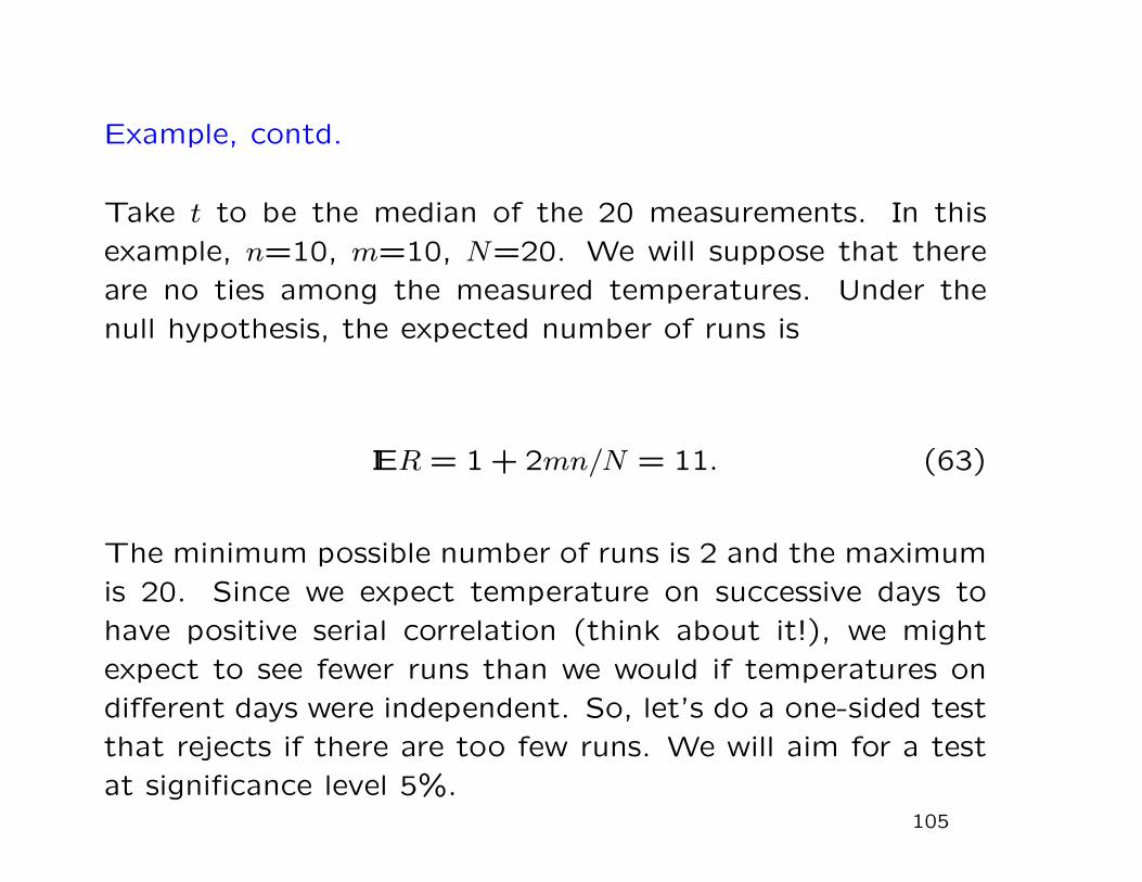
Example, contd.
Take t to be the median of the 20 measurements. In this
example, n=10, m=10, N=20. We will suppose that there
are no ties among the measured temperatures. Under the
null hypothesis, the expected number of runs is
IER = 1 + 2mn/N = 11. (63)
The minimum possible number of runs is 2 and the maximum
is 20. Since we expect temperature on successive days to
have positive serial correlation (think about it!), we might
expect to see fewer runs than we would if temperatures on
different days were independent. So, let’s do a one-sided test
that rejects if there are too few runs. We will aim for a test
at significance level 5%.105
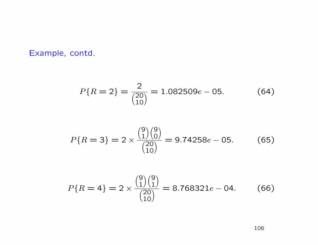
Example, contd.
PR = 2 =2(2010
) = 1.082509e− 05. (64)
PR = 3 = 2×
(91
)(90
)(
2010
) = 9.74258e− 05. (65)
PR = 4 = 2×
(91
)(91
)(
2010
) = 8.768321e− 04. (66)
106
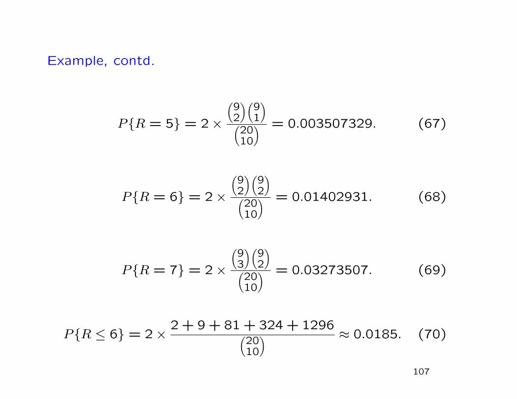
Example, contd.
PR = 5 = 2×
(92
)(91
)(
2010
) = 0.003507329. (67)
PR = 6 = 2×
(92
)(92
)(
2010
) = 0.01402931. (68)
PR = 7 = 2×
(93
)(92
)(
2010
) = 0.03273507. (69)
PR ≤ 6 = 2×2 + 9 + 81 + 324 + 1296(
2010
) ≈ 0.0185. (70)
107
Example, contd.
So, we should reject the null hypothesis if R ≤ 6, which
gives a significance level of 1.9%. Including R = 7 in the
rejection region would make the significance level slightly too
big: 5.1%.
108
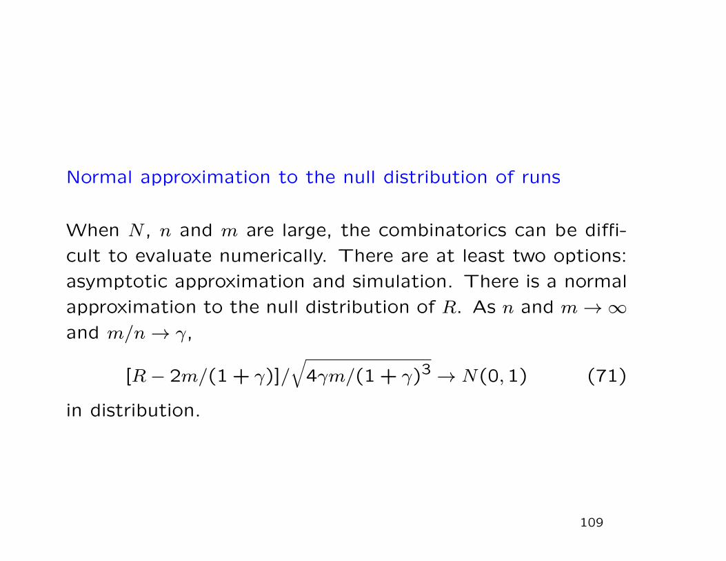
Normal approximation to the null distribution of runs
When N , n and m are large, the combinatorics can be diffi-
cult to evaluate numerically. There are at least two options:
asymptotic approximation and simulation. There is a normal
approximation to the null distribution of R. As n and m→∞and m/n→ γ,
[R− 2m/(1 + γ)]/√
4γm/(1 + γ)3 → N(0,1) (71)
in distribution.
109

Code for runs test
Here is an R function to simulate the null distribution of the
number R of runs, and evaluate the P -value of the observed
value of R conditional on n, for a one-sided test against the
alternative that the distribution produces fewer runs than in-
dependent trials would tend to produce. The input is a vec-
tor of length N ; each element is equal to either “1” (heads)
or “-1” (tails). The test statistic is calculated by finding
1 +∑N−1j=1 Ij, as we did above in finding IER.
110
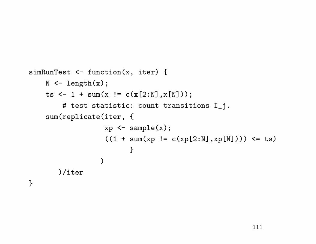
simRunTest <- function(x, iter)
N <- length(x);
ts <- 1 + sum(x != c(x[2:N],x[N]));
# test statistic: count transitions I_j.
sum(replicate(iter,
xp <- sample(x);
((1 + sum(xp != c(xp[2:N],xp[N]))) <= ts)
)
)/iter
111
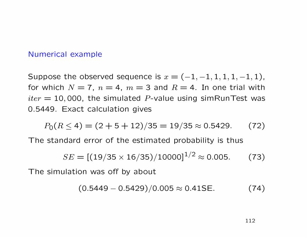
Numerical example
Suppose the observed sequence is x = (−1,−1,1,1,1,−1,1),
for which N = 7, n = 4, m = 3 and R = 4. In one trial with
iter = 10,000, the simulated P -value using simRunTest was
0.5449. Exact calculation gives
P0(R ≤ 4) = (2 + 5 + 12)/35 = 19/35 ≈ 0.5429. (72)
The standard error of the estimated probability is thus
SE = [(19/35× 16/35)/10000]1/2 ≈ 0.005. (73)
The simulation was off by about
(0.5449− 0.5429)/0.005 ≈ 0.41SE. (74)
112
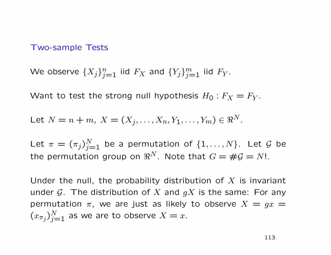
Two-sample Tests
We observe Xjnj=1 iid FX and Yjmj=1 iid FY .
Want to test the strong null hypothesis H0 : FX = FY .
Let N = n+m, X = (Xj, . . . , Xn, Y1, . . . , Ym) ∈ <N .
Let π = (πj)Nj=1 be a permutation of 1, . . . , N. Let G be
the permutation group on <N . Note that G = #G = N !.
Under the null, the probability distribution of X is invariant
under G. The distribution of X and gX is the same: For any
permutation π, we are just as likely to observe X = gx =
(xπj)Nj=1 as we are to observe X = x.
113

Permutation group
G = #G = N ! (75)
#gx : g ∈ G ≤ N ! (76)
(less than N ! if x has repeated components).
#T (gx) : g ∈ G ≤#gx : g ∈ G ≤ N ! (77)
will be much less than(Nn
)if T only cares about sets assigned
to the first n components and to the last m components, not
the ordering within those sets.
114
“Impartial” use of the data: Arrangements
An “arrangement” of the data is a partition of it into twosets, n considered to be from the first (X) population andm considered to be from the second (Y ) population. In anarrangement, the order of the values within each of thosetwo sets does not matter.
Some statisticians require the test statistic to be “impartial”:Since Xj are iid and Yj are iid, statistic shouldn’t privilegesome Xj or Yj over others. The labeling is considered to bearbitrary.
Not compelling for sequential methods, where the labelingcould indicate the order in which the observations were made.
For the test statistics we consider, only the arrangement mat-ters: They are impartial.
115

Unbiased tests
A test is unbiased if the chance it rejects the null is never
smaller when the null is false than when the null is true.
116
Testing whether IEFX = IEFY
FX = FY implies IEFX = IEFY , but not vice versa. Weaker
hypothesis.
Start with strong null that FX = FY , but want test to be sen-
sitive to differences between IEFX and IEFY . We are testing
the strong null, but we want power against the alternative
IEFX 6= IEFY .
Test statistic. Let X ≡ 1n
∑nj=1Xj and Y ≡ 1
m
∑mj=1 Yj.
Tn,m(X) = Tn,m(X1, . . . , Xn, Y1, . . . , Ym) ≡ n1/2(X − Y ) (78)
To test, if we observe X = x, look at the values of Tn,m(gx) :
g ∈ G. We reject if T (x) is “extreme” compared with those
values.117
Distribution of Tn,m without invariance
Romano [?] shows that if IEFX = IEFY = µ, if FX and FYhave finite variances, and if m/N → λ ∈ (0,1) as n→∞, then
the asymptotic distribution of Tn,m is normal with mean zero
and variance
σ2p = λ−1/2(λVarFY + (1− λ)VarFX). (79)
The permutation distribution and unconditional asymptotic
distributions are equal only if VarFX = VarFY or λ = 1/2.
Hence, whether the test is asymptotically valid for the “weak”
null hypothesis depends on the relative sample sizes.
118
Pitman’s papers
[?, ?, ?]
Paper 1: Two-sample test for equality of two distribution
based on sample mean. This is what we just looked at.
Paper 2: correlation by permutation. Exchangeability re-
quired. Issues for time series in particular.
Paper 3: ANOVA by permutation.
119
Permutation test for association
Observe (Xj, Yj)nj=1. Xjnj=1 are iid and Yjnj=1 are iid.
The pairs are independent of each other; the question is
whether, within pairs, X and Y are independent.
If they were, the joint distribution of (Xj, Yj)nj=1 would be
the same as the joint distribution of (Xj, Yπj)nj=1 for ev-
ery permutation π of 1, . . . , n. The joint distribution of
(Xj, Yj)nj=1 would be invariant under the group of permu-
tations of the indices of the Y variables.
The Y s would be exchangeable given the Xs. Exchangeability
involves not just the independence of X and Y , but also the
fact that the Y s are iid. If they had different distributions or
were dependent, exchangeability would not hold.120
Test Statistic
Testing the null hypothesis that Yj are exchangeable given
Xj, which is implied by the assumption that Yj are iid,
combined with the null that Xj are independent of Yj.
Can treat either Xj or Yj as fixed numbers—not neces-
sarily random. For instance, Xj could index deterministic
locations at which the observations Yj were made.
The issue is whether, conditional on one of the variables, all
pairings with the other variable are equally likely.
We want to be sensitive to violations of the null for which
there is dependence within pairs. One statistic that is sensi-
121
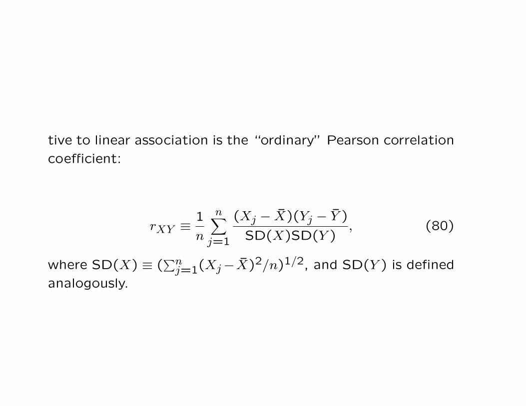
tive to linear association is the “ordinary” Pearson correlation
coefficient:
rXY ≡1
n
n∑j=1
(Xj − X)(Yj − Y )
SD(X)SD(Y ), (80)
where SD(X) ≡ (∑nj=1(Xj−X)2/n)1/2, and SD(Y ) is defined
analogously.

Example: acclamations and coinage symbols
Example from Norena [?].
Roman emperors were “acclaimed” with various honors dur-
ing their reigns. Coins minted in their reigns have a variety
of symbols, one of which is Victoria (symbolizing military
victory). (Coins recovered from various caches; assumed to
be a representative sample—which is not entirely plausible.)
Look at emperors from the year 96 to 218.
122
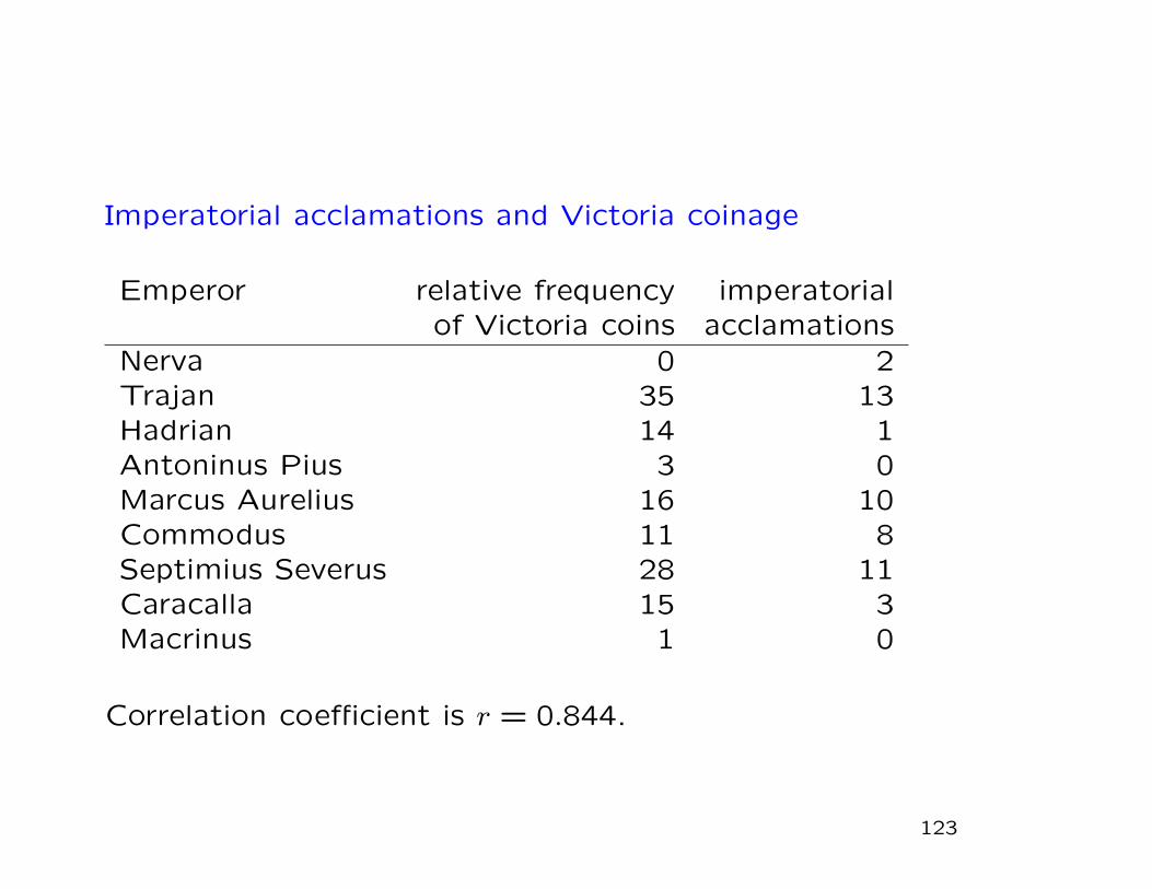
Imperatorial acclamations and Victoria coinage
Emperor relative frequency imperatorialof Victoria coins acclamations
Nerva 0 2Trajan 35 13Hadrian 14 1Antoninus Pius 3 0Marcus Aurelius 16 10Commodus 11 8Septimius Severus 28 11Caracalla 15 3Macrinus 1 0
Correlation coefficient is r = 0.844.
123
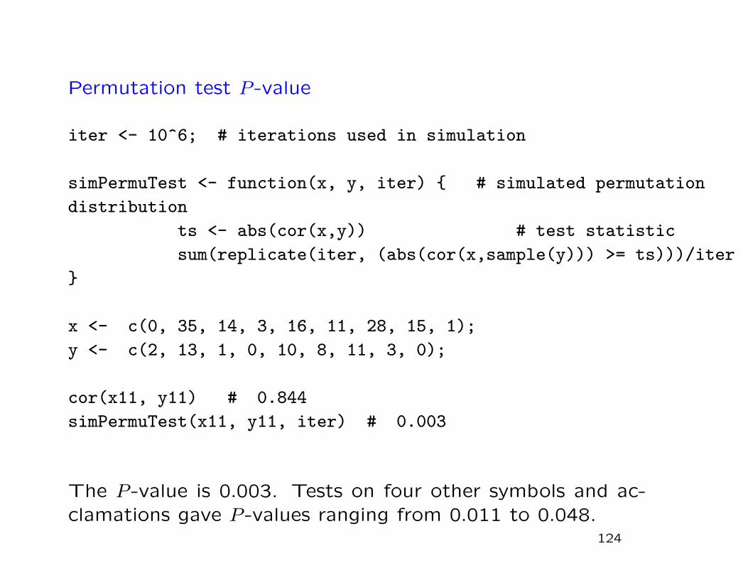
Permutation test P -value
iter <- 10^6; # iterations used in simulation
simPermuTest <- function(x, y, iter) # simulated permutation
distribution
ts <- abs(cor(x,y)) # test statistic
sum(replicate(iter, (abs(cor(x,sample(y))) >= ts)))/iter
x <- c(0, 35, 14, 3, 16, 11, 28, 15, 1);
y <- c(2, 13, 1, 0, 10, 8, 11, 3, 0);
cor(x11, y11) # 0.844
simPermuTest(x11, y11, iter) # 0.003
The P -value is 0.003. Tests on four other symbols and ac-clamations gave P -values ranging from 0.011 to 0.048.
124

Spearman’s Rank Correlation
Test statistic: replace each Xj by its rank and each Yj by
its rank. Test statistic is the correlation coefficient of those
ranks. This is Spearman’s rank correlation coefficient, de-
noted rS(X,Y ).
Significance level from the distribution of the statistic under
permutations, as above.
Can use midranks to deal with tied observations.
125
What if Yj are dependent or have different distributions?
In time series context where j indexes time, typical that Yjhave different distributions and are dependent.
Trends, cycles, etc., correspond to different means at differ-
ent times. Variances can depend on time, too. So can other
aspects of the distribution.
126
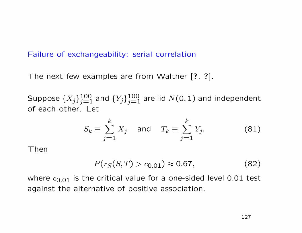
Failure of exchangeability: serial correlation
The next few examples are from Walther [?, ?].
Suppose Xj100j=1 and Yj100
j=1 are iid N(0,1) and independent
of each other. Let
Sk ≡k∑
j=1
Xj and Tk ≡k∑
j=1
Yj. (81)
Then
P (rS(S, T ) > c0.01) ≈ 0.67, (82)
where c0.01 is the critical value for a one-sided level 0.01 test
against the alternative of positive association.
127
Serial correlation, contd.
Even though Sj and Tj are independent, the probability
that their Spearman rank correlation coefficient exceeds the
0.01 critical value for the test is over 2/3.
That is because the two series S and T each have serial
correlation: not all pairings (Sj, Tπj) are equally likely—even
though the two series are independent. The series are not
conditionally exchangeable even though they are indepen-
dent, because neither series is iid.
128

Failure of exchangeability: difference in variances
Serial correlation is not the only way that exchangeability can
fail. For example, if the mean or the noise level varies with
time, that violates the null hypothesis.
Take X = (1,2,3,4) fixed. Let (Y1, Y2, Y3, Y4) be indepen-
dent, jointly Gaussian with zero mean, σ(Yj) = 1, j = 1,2,3,
and σ(Y4) = 2. If Yj were exchangeable—which they are
not—then
P0(rS(X,Y ) = 1) = 1/4! = 1/24 ≈ 4.17%. (83)
(rS = 1 whenever Y1 < Y2 < Y3 < Y4.) Simulation shows that
P (rS(X,Y ) = 1) ≈ 7%:
129
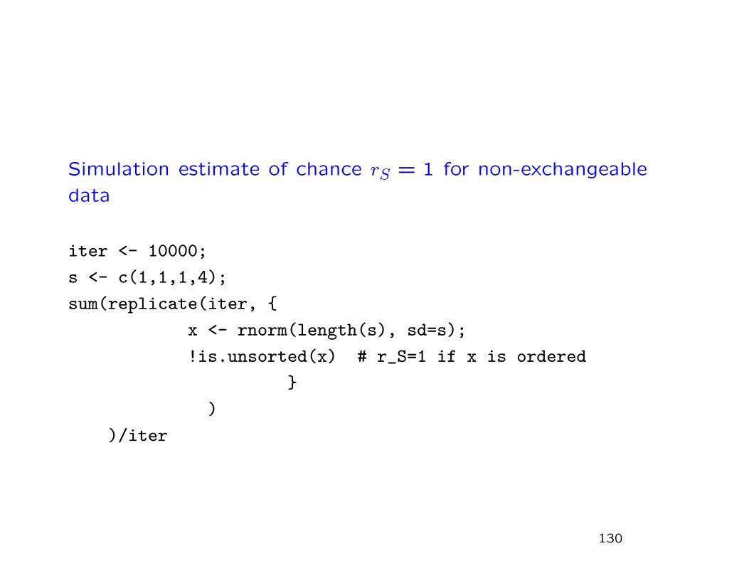
Simulation estimate of chance rS = 1 for non-exchangeable
data
iter <- 10000;
s <- c(1,1,1,4);
sum(replicate(iter,
x <- rnorm(length(s), sd=s);
!is.unsorted(x) # r_S=1 if x is ordered
)
)/iter
130

Failure of exchangeability: difference in variances
Take X = (1,2,3,4,5) fixed, let (Y1, Y2, Y3, Y4, Y5) be inde-
pendent, jointly Gaussian with zero mean and standard devi-
ations 1, 1, 1, 3, and 5, respectively.
Under the (false) null hypothesis that all pairings (Xj, Yπj)are equally likely,
P0rS(X,Y ) = 1 = 1/5! ≈ 0.83%, (84)
Simulation shows that the actual probability is about 2.1%.
In these examples, the null hypothesis is false, but not be-
cause Xj and Yj are dependent. It is false because not
all pairings (Xj, Yπj) are equally likely. The “identically dis-
tributed” part of the null hypothesis fails.
131
Failure of exchangeability: difference in means
Xj = j, ... [FIX ME!]
132
Permutation F -test
We have m batches of n subjects, not necessarily a sample
from any larger population.
In each batch, the n subjects are assigned to n treatments
at random. Let rjk be the response of the subject in batch j
who was assigned to treatment k, j = 1, . . . ,m, k = 1, . . . , n.
Linear model:
rjk = Bj + Tk + ejk. (85)
Bj is a “batch effect” that is the same for all subjects in batch
j. Tk is the effect of treatment k. ejk is an observational error
for the individual in batch j assigned to treatment k.
Want to test the null hypothesis that T1 = T2 = . . . = Tn.133
ANOVA
Decompose total sum of squares:
S = SB + ST + Se, (86)
where SB is independent of the treatments, ST is independent
of the batches, and Se is the residual sum of squares, and is
independent of batches and of treatments.
Test statistic
F =ST
ST + Se. (87)
Large if the “within-batch” variation can be accounted for
primarily by an additive treatment effect.
In usual F -test, assume that ejk are iid normal with mean
zero, common variance σ2.134
ANOVA “ticket model”
Each individual is represented by a ticket with n numberson it. The kth number on ticket m is the response thatindividual m would have if assigned to treatment k. We as-sume non-interference: each individual’s potential responsesare summarized by those n numbers; they do not depend onwhich treatment any other subjects are given.
If treatment has no effect whatsoever, then, individual m’sn numbers are all equal. That is, within each batch, thetreatment label is arbitrary. Responses should be invariantunder permutations of the treatment labels.
Let πj be a permutation of 1, . . . , n, for j = 1, . . . ,m. If weobserve rjk and the null is true, we might just as well haveobserved r
jπjk
Keep batches together, but permute the treatment labelswithin batches.
135

Permutation distribution
Condition on the event that the data are in the orbit of the
observed data under the action of the permutation group.
Then all points in that orbit are equally likely.
Find the P -value by comparing the observed value of F with
the distribution of values in the orbit of the observed data un-
der the group that permutes the labelings within each batch.
Reject the null hypothesis if the observed value of F is sur-
prisingly large.
If the space of permutations is too big, can use randomly
selected permutations.
136
How strong is the usual null for the F -test?
The permutation test just described tests the strong null that
the n numbers on individual m’s ticket are equal. A weaker
null that might be of interest is whether the n means of
the mn potential responses to each of the n treatments are
equal—that is, whether on average there is any difference
among the treatments.
Does the usual F -test test this weaker null? What hypothesis
does the F -test actually address?
137
F -test null hypothesis
For F to have an F -distribution, the “noise” terms ejkhave to be iid normal random variables with mean zero (thatmakes it the ratio of two chi-square variables if the treatmenteffects are equal). The distribution of ejk cannot dependon which batch the subject is in nor which treatment thesubject receives.
Why should each ejk have expected value zero? Why shouldejk be independent of the assignment to treatment? Whyshould ejk have the same distribution for all individuals?
Why should the effect of a given treatment be the same forevery individual?
Why is there no interaction between treatment and batch?
Why is the “batch effect” the same for all members of abatch?
138
Sharpening the description
To study whether different treatments have different effects,
need to consider hypothetical counterfactuals.
What would the response of the individual in batch j assigned
to treatment k have been, if the individual instead had been
assigned to treatment ` 6= k?
The model
rjk = Bj + Tk + ejk (88)
doesn’t say. We need a “response schedule” [?].
139
Response schedule
Think of the subjects within batches before they are assigned
to treatment. The response schedule says that if subject `
in batch j is assigned to treatment k, his response will be
r` = Bj + Tk + e`. (89)
If he is assigned to treatment k′, his response will be
r` = Bj + Tk′ + e`. (90)
How is e` generated? Would e` be the same if subject ` were
assigned to treatment k′ instead of treatment k?
140
Two visions of e`: Vision 1
The errors e` are generated (iid Normal, mean zero) before
the subjects are assigned to treatments. Once generated,
e` are intrinsic properties of the individuals—unaffected by
assignment to treatment. And the assignment to treatment
does not depend on e`.
If this is true, then if the treatment effects Tk are all equal,
that implies more than the strong null: Within each batch,
each individual’s responses would be the same no matter
which treatment was assigned—the n numbers on each in-
dividual’s ticket are equal, just as in the strong null. But in
addition, the expected responses of all subjects in each batch
are equal.
141
Two visions of e`: Vision 2
e` are generated after the assignment to batch and treat-
ment, but their distribution does not depend on that assign-
ment. If the assignment had been different, e` might have
been different—but it is always Normal with zero mean and
the same variance, and never depends on the assignment of
that subject or any other subject.
If this is true, then the null that the treatment effects Tk are
all equal implies a weakening of the null: Within each batch,
each individual’s responses are the same in expectation no
matter which treatment is assigned, but a given individual
might have n different numbers on his ticket.
142
Two visions of e`: Vision 2, contd.
However, the hypothesis says more than that: Within each
batch, every subject’s expected response is the same—the
same as the expected response of all the other subjects, no
matter which treatment is assigned to each of them.
This seems rather stronger than the “strong null” that the
permutation test tests, since the strong null does not require
different subjects to have the same expected responses.
Note that in neither vision 1 nor vision 2 is the null the “natu-
ral” weak null that the average of the responses (across sub-
jects) for each treatment are equal, even though the numbers
are not necessarily equal subject by subject.
143
Other test statistics
The F statistic makes sense for testing against the omnibusalternative that there is a difference among the treatmenteffects.
If there is more structure to the alternative, can devise testswith more power against the alternative.
For instance, if, under the alternative, the treatment effectsare ordered, can use a test statistic that is sensitive to theorder. Suppose that the treatments are ordered so if thealternative is true, T1 ≤ T2 ≤ · · · ≤ Tn.
Pitman correlation
S ≡n∑
k=1
f(k)m∑j=1
rjk (91)
where f is a monotone increasing function.144

Most powerful permutation tests
How should we select the rejection region?
If we have a simple null and a simple alternative, most pow-
erful test is likelihood ratio test.
If the null completely specifies the chance of outcomes in the
orbit of the data and the alternative does too, can find the
likelihood ratio for each point in the orbit.
Problem: The orbits might not be the same under the null
and under the alternative. If they were the same, the chance
of each outcome in the orbit would be the same under the
two hypotheses, since the elements of the orbit are equally
likely.
145
Example: incompatible orbits
6 subjects; 3 assigned to treatment and 3 to control, at
random.
Null: treatment has no effect at all.
Alternative: treatment increases the response by 1 unit.
Data: responses to control 1,2,3. Responses to treatment
2,3.5,4.
Under the null, the orbit consists of the 20 ways of partition-
ing 1,2,2,3,3.5,4 into two groups of 3; equivalently, the 6!
permutations of 1,2,2,3,3.5,4.
146

Example: incompatible orbits, contd.
Under the alternative, the orbit consists of 20 points, but
they are generated differently: Find the responses that would
have been observed if none had been assigned to treatment
by subtracting the hypothesized treatment effect. That gives
1,1,2,2.5,3,3.
Take 1,1,2,2.5,3,3 and partition it into two groups of 3;
add 1 to each element of the second group. Equivalently,
take each of the 6! permutations of 1,1,2,2.5,3,3 and add
1 to the last 3 elements.
147
Example: incompatible orbits, contd.
Under the null, one element of the orbit is (1,2,2,3,3.5,4).
That point is not in the orbit under the alternative.
Under the alternative, one element of the orbit is (1,1,2,3.5,4,4).
That point is not in the orbit under the null.
Most powerful test would have in its rejection region those
points that are in the orbit under the null but not in the orbit
under the alternative, since for those points, the likelihood
ratio is infinite. Hot helpful.
What are we conditioning on? If we condition on the event
that the data are in the orbit of the observed data, can’t do
much.
148

Most Powerful Permutation Tests
See Lehmann and Romano [?], pp. 177ff. [FIX ME!]
149
The Population Model
We’ve been taking N subjects as given; the assignment to
treatment or control was random.
Now consider instead the N subjects to be random samples
from two populations.
Observe Xjnj=1 iid FX and Yjmj=1 iid FY .
Want to test the hypothesis FX = FY .
150

Many scenarios give rise to the same conditional null distri-
bution for the permutation test:
• Randomization model for comparing two treatments. N
subjects are given and fixed; n are assigned at random to
treatment and m = N − n to control.
• Population model for comparing two treatments. N sub-
jects are a drawn as a simple random sample from a much
larger population; n are assigned at random to treatment
and m = N − n to control.
151
• Comparing two sub-populations using a sample from each.
A simple random sample of n subjects is drawn from one
much larger population with many more than N members,
and a simple random sample of m subjects is drawn from
another population with many more than m members.
• Comparing two sub-populations using a sample from the
pooled population. A simple random sample of N sub-
jects is drawn from the pooled population, giving random
samples from the two populations with random sample
sizes. Condition on the sample sizes n and m.
• Comparing two sets of measurements. Independent sets
of n and m measurements come from two sources. Test
hypothesis that the two sources have the same distribu-
tion.
152

In all those scenarios, if the null hypothesis is true the data
are exchangeable—the distribution is invariant under permu-
tations.
Hence, a test with the right (conditional) level for one sce-
nario can be applied in all the others.
153

Aside: stochastic ordering
Suppose X and Y are real-valued random variables. X is
stochastically larger than Y , written Y X, if
PrX ≥ x ≥ PrY ≥ x ∀x ∈ <. (92)
Exercise: Show that Y X if and only if for every mono-
tonically increasing function u, IEu(Y ) ≤ IEu(X).
154
Example of a power estimate: stochastic ordering
Observe Xjnj=1 iid FX and Yjmj=1 iid FY .
Under the null, FX = FY .
Under the alternative FX is stochastically than FY .
Test at level α using the sample mean as the test statistic.
What’s the chance of rejecting the null if the alternative is
true?
155
Aside: the Probability Transform
Let X be a real-valued random variable with continuous cdf
F .
Then F (X) ∼ U [0,1].
Proof: Note that F (X) ∈ [0,1]. If F is continuous, for
p ∈ (0,1) there is a unique value xp ∈ < such that F (xp) = p.
(That is, F has an inverse function F−1 on (0,1).)
For any p ∈ (0,1),
PrF (X) ≤ p = PrX ≤ xp = p. (93)
But this is exactly what it means to have a uniform distribu-
tion.
Patch for non-necessarily continuous F? See below.156
Aside: a useful stochastic ordering lemma (From [?]; see
also [?].)
X is stochastically larger than Y iff there is a random variable
W and monotone nondecreasing functions f and g such that
g(x) ≤ f(x) for all x, g(W ) ∼ Y and f(W ) ∼ X.
Proof: Suppose Y X. Let FX be the cdf of X and let FYbe the cdf of Y . Define
f(p) ≡ infx : FX(x) ≥ p and g(p) ≡ infx : FY (x) ≥ p.(94)
Then f and g are nondecreasing functions on [0,1]. Since
FY (x) ≤ FX(x), it follows that g(p) ≤ f(p).
157
Proof of lemma, contd.
(a) If p ≤ FX(x), then f(p) ≤ f(FX(x)) ≤ x. (The firstinequality follows from the monotonicity of f ; the secondfrom the fact that FX is nondecreasing but can be flat onsome intervals. Hence, the smallest y for which FX(y) ≥FX(x) can be smaller than x.)
(b) If f(p) ≤ x then FX(f(p)) ≤ FX(x), and hence p ≤ FX(x).(The first inequality follows from the monotonicity of F ; thesecond from the fact that f is the infimum.)
Let W ∼ U [0,1]. By (a),
FX(x) = PrW ≤ FX(x) ≤ Prf(W ) ≤ x. (95)
By (b),
Prf(W ) ≤ x ≤ PrW ≤ FX(x) = FX(x). (96)
Hence Prf(W ) ≤ x = FX(x): f(W ) ∼ FX. Similarly,g(W ) ∼ FY .
158
Proof of lemma, contd.
In the other direction, suppose there is a random variable
W and monotone nondecreasing functions f and g such that
g(x) ≤ f(x) for all x, g(W ) ∼ Y and f(W ) ∼ X.
Then
PrX ≥ x = Prf(W ) ≥ x ≥ Prg(W ) ≥ x = PrY ≥ x.(97)
159
Consequence of the lemma
Let Xjnj=1 iid with cdf FX and Yjmj=1 iid with cdf FY , withFX and FY continuous. Let N = n+m.
Let X = (X1, . . . , Xn, Y1, . . . , Ym) ∈ <N . Let φ : <N → [0,1].Suppose that φ satisfies two constraints:
(a) If FX = FY then
IEφ(X) = α, (98)
so that φ is the test function for a level α test of the hypoth-esis FX = FY .
(b) If xj ≤ x′j, j = 1, . . . , n, then
φ(x1, . . . , xn, y1, . . . , ym) ≤ φ(x′1, . . . , x′n, y1, . . . , ym). (99)
Then IEφ ≥ α whenever FY FX.160
Proof of consequence
By the lemma, there are nondecreasing functions g ≤ f and iid
random variables WjNj=1 such that f(Wj) ∼ FX and g(Wj) ∼FY .
By (a),
IEφ(g(W1), . . . , g(Wn), g(Wn+1), . . . , g(WN)) = α. (100)
By (b),
IEφ(f(W1), . . . , f(Wn), g(Wn+1), . . . , g(WN)) = β ≥ α. (101)
161

The permutation test based on the sample mean is unbiased
under the alternative of stochastic dominance
Suppose Xjnj=1 are iid with cdf FX and Yjmj=1 are iid
with cdf FY . Define the test function φ so that φ(X) =
1 iff∑nj=1Xj (or 1
n
∑nj=1Xj) is greater than the sum (or
mean, respectively) of the first n elements of αN ! of the N !
(not necessarily distinguishable) permutations of the multiset
[X1, . . . , Xn, Y1, . . . , Ym].
Define the power function
β(FX , FY ) = IEφ(X1, . . . , Xn, Y1, . . . , Ym). (102)
Then β(FX , FX) = α and β(FX , FY ) ≥ α for all pairs of distri-
butions for which FX is stochastically larger than FY .
162
Proof.
We have already proved that β(FX , FX) = α: The permuta-
tion test is exact (possibly requiring randomization, depend-
ing on α).
To show that β(FX , FY ) > α, suppose that the observed value
of Xj is xj, the observed value of Yj is yj, and let w =
(x1, . . . , xn, y1, . . . , ym) ∈ <N .
φ = 1 if∑nj=1wj is sufficiently large compared with
∑nj=1wπj
for enough permutations π.
Want to show that Prφ = 1 is larger when FY FX than
when FY = FX.
163
By the lemma, suffices to show that if xj ≤ x′j, j = 1, . . . , n,
then
φ(x1, . . . , xn, y1, . . . , ym) ≤ φ(x′1, . . . , x′n, y1, . . . , ym). (103)
I.e., suffices to show that if we would reject the null for data
w = (x1, . . . , xn, y1, . . . , ym), (104)
we would also reject it for data
w′ = (x′1, . . . , x′n, y1, . . . , ym). (105)
Suppose φ(w) = 1. Then∑nj=1wj >
∑nj=1wπj for at least
αN ! of the permutations π of 1, . . . , N. Let π be one such
permutation.
164
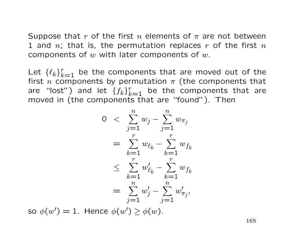
Suppose that r of the first n elements of π are not between1 and n; that is, the permutation replaces r of the first ncomponents of w with later components of w.
Let `krk=1 be the components that are moved out of thefirst n components by permutation π (the components thatare “lost”) and let fkrk=1 be the components that aremoved in (the components that are “found”). Then
0 <n∑
j=1
wj −n∑
j=1
wπj
=r∑
k=1
w`k −r∑
k=1
wfk
≤r∑
k=1
w′`k −r∑
k=1
wfk
=n∑
j=1
w′j −n∑
j=1
w′πj ,
so φ(w′) = 1. Hence φ(w′) ≥ φ(w).165
Estimating shifts:
If you know that FX(x) = FY (x − d), can construct a confi-
dence interval for the shift d.
How?
Invert hypothesis tests.
166
Exercise:
By simulation, estimate the power of the level α = 0.05 two-
sample test based on the sample mean against the alternative
that FY FX when
1. Y ∼ N(0,1) and X ∼ N(µ,1), µ = 0.5,1,1.5. Compare
with the power of the usual t test.
2. Y ∼ Exponential(1) and X ∼ Exponential(λ), with 1/λ =
1.5,2,2.5. Compare with the power of a likelihood ratio
test.
3. Y ∼ Chi-square(2) and X ∼ Chi-square(b), with b =
3,4,5. Compare with the power of a likelihood ratio test.
167

Exercise, contd.
Use sample sizes n = 10,50,100 and m = n/2, n, and 2n.
Justify your choice of the number of replications to use in
each simulation. Note: this involves 81 simulations. Please
tabulate the results in some readable format.
For each of the scenarios above, pretend that FX(x) = FY (x−d) for some shift d that could be positive or negative. (This
is true in the first scenario where the data are normal with
different means, but not in the second and third, where the
distributions have different shapes.) Invert two-sided tests
to find 95% confidence intervals for d, which would be the
difference in means if the shift model were true. By simu-
lation, estimate the probability that the confidence intervals
cover the true difference in means in the 81 cases. Justify
your choice of the number of replications to use in each sim-
ulation. Discuss the results.168
Smirnov Test
Consider a two-sample test against the omnibus alternative
that there is any difference at all between the two groups.
We want a test statistic that is sensitive to differences other
than differences in the means.
The Smirnov test is based on the difference between the em-
pirical cumulative distribution function (cdf) of the treatment
responses and the empirical cdf of the control responses. It
has some power against all kinds of violations of the strong
null hypothesis.
169
Smirnov Test, contd. Let FX,n denote the empirical cdf of
the treatment responses:
FX,n(x) ≡#xj : xj ≤ x/n, (106)
and define FY,m analogously as the empirical cdf of the control
responses. If there are no ties within the treatment group,
FX,n jumps by 1/n at each treatment response value. If there
are no ties within the control group, FY,m jumps by 1/m at
each control response value. If k of the treatment responses
are tied and equal to x0, then FX,n jumps by k/n at x0.
170
Smirnov Test, contd.
The Smirnov test statistic is
Dm,n ≡ supx|FX,n(x)− FY,m(x)|. (107)
It is easy to see that the supremum is attained at one of the
data values. We can also see that the supremum depends
only on the ranks of the data, because the order of the jumps
matters, but the precise values of x at which the jumps occur
do not matter. Therefore, the test
Reject null if Dm,n > c, (108)
for an appropriately chosen value of c, is a nonparametric test
of the strong null hypothesis.
171

Smirnov Test, contd.
Null distribution of Dm,n for n = 3, m = 2. There are(53
)= 10 possible assignments of 3 of the subjects to treat-
ment, each of which has probability 1/10 under the strongnull hypothesis. Assume that the 5 data are distinct (no ties).Then the possible values of Dm,n are
treatment ranks control ranks Dm,n1,2,3 4,5 11,2,4 3,5 2/31,2,5 3,4 2/31,3,4 2,5 1/21,3,5 2,4 1/31,4,5 2,3 2/32,3,4 1,5 1/22,3,5 1,4 1/22,4,5 1,3 2/33,4,5 1,2 1
172
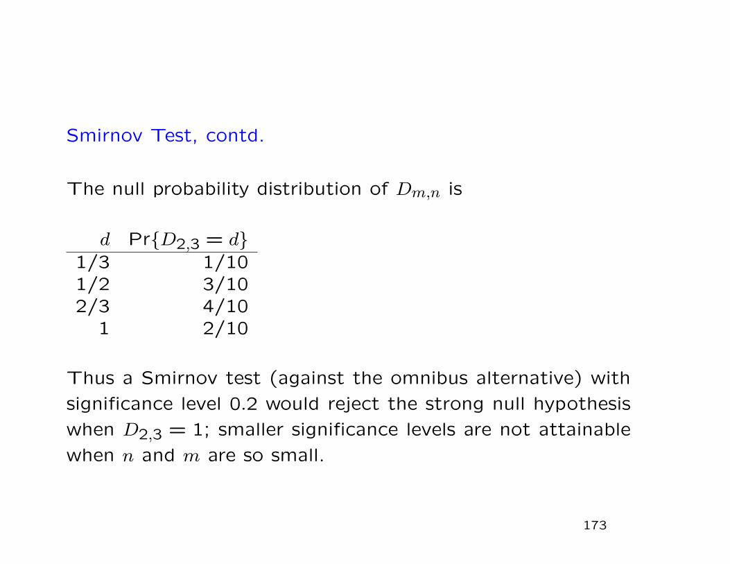
Smirnov Test, contd.
The null probability distribution of Dm,n is
d PrD2,3 = d1/3 1/101/2 3/102/3 4/10
1 2/10
Thus a Smirnov test (against the omnibus alternative) with
significance level 0.2 would reject the strong null hypothesis
when D2,3 = 1; smaller significance levels are not attainable
when n and m are so small.
173
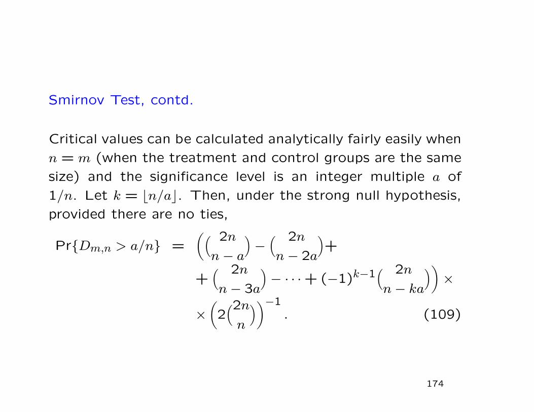
Smirnov Test, contd.
Critical values can be calculated analytically fairly easily when
n = m (when the treatment and control groups are the same
size) and the significance level is an integer multiple a of
1/n. Let k = bn/ac. Then, under the strong null hypothesis,
provided there are no ties,
PrDm,n > a/n =(( 2n
n− a
)−( 2n
n− 2a
)+
+( 2n
n− 3a
)− · · ·+ (−1)k−1
( 2n
n− ka
))×
×(
2(2nn
))−1. (109)
174
Smirnov Test, contd.
When there are ties, Dm,n tends to be smaller, so tail prob-
abilities from this expression still give conservative tests. (If
both members of a tie are assigned to the same group (treat-
ment or control) the tie does not change the value of Dm,nfrom the value it would have had if the pair differed slightly.
If one member of a tie is assigned to treatment and one to
control, the tie can decrease the value of Dm,n from the value
it would have had if the observations differed slightly. Thus
Dm,n is stochastically smaller when there are ties.
175
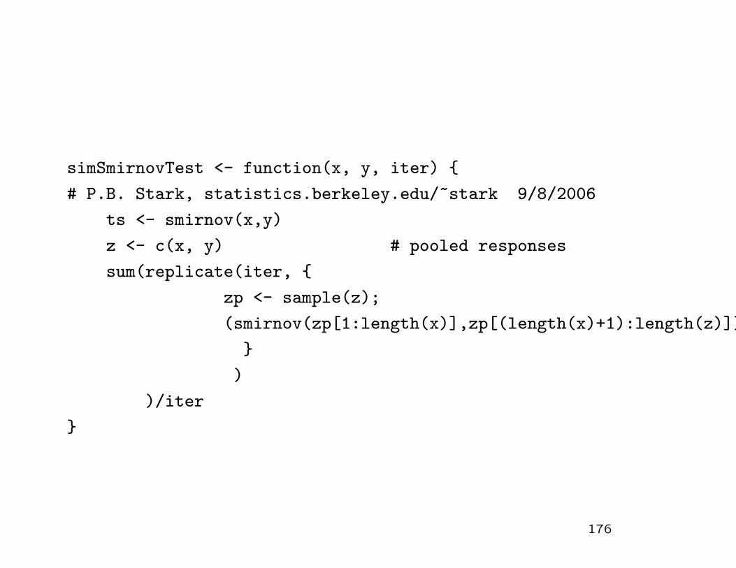
simSmirnovTest <- function(x, y, iter)
# P.B. Stark, statistics.berkeley.edu/~stark 9/8/2006
ts <- smirnov(x,y)
z <- c(x, y) # pooled responses
sum(replicate(iter,
zp <- sample(z);
(smirnov(zp[1:length(x)],zp[(length(x)+1):length(z)]) >= ts)
)
)/iter
176
We can also estimate the power of the Smirnov statistic
against a shift alternative by simulation. Suppose that the
effect of treatment is to increase each subject’s response by
d, no matter what the response would have been in con-
trol. (Remember, this is a very restrictive assumption, but
the results might be suggestive anyway.) Then the responses
x = (xj)nj=1 of the treated subjects would have been
x− d = (x1 − d, . . . , xn − d) (110)
had they been in the control group, and the responses y of
the control group would have been y + d had they been in
the treatment group.
See old lecture notes, chapter 4.
177

Multidimensional analogues?
Test statistics: sample mean versus ...
Multidimensional analogue of the runs test: deleting edges
from minimal spanning tree. Depends on metric.
Bickel [?] probability of lower-left quadrants.
Friedman and Rafsky [?] generalized “runs” test based in
minimal spanning trees.
Ferger [?] change point at known point.
Hall and Tajvidi [?] inter-point differences to each point.
178

Baringhaus and Franz [?] sum of interpoint differences acrosssamples minus half the sums of interpoint differences withinsamples.
Multidimensional analogues of the Smirnov test: VC classes,Romano’s work.
Gretton et al. [?] generalizes from indicator functions of setsto expectation of more general functions (e.g., elements of auniversal reproducing kernel Hilbert space). Good propertiesif the star of the set of functions is dense in C0 in the L∞norm.
Median versus mean.
Testing the hypothesis of symmetry.
Testing exchangeability: earthquake aftershocks.
The two-sample problem
We observe Xjnj=1 iid P and Yjmj=1 iid Q.
P and Q are measures on a common sigma-algebra A.
Want to test the hypothesis P = Q.
(Recall that the math is essentially the same whether the two
samples are random samples from two populations, measure-
ments on a single group randomly divided into treatment and
control, or—conditional on the sample sizes—a single ran-
dom sample from a population with two types of elements.)
179

The two-sample problem in IRp
For x ∈ IRp, define the lower left quadrant w.r.t. x:
Lx ≡ y ∈ IRp : yj ≤ xj, j = 1, . . . , p. (111)
Let
δ(P,Q) ≡ supx∈IRp
|P (Lx)−Q(Lx)| (112)
Bickel [?] shows that the permutation principle applied to
the test statistic δ(P , Q) gives a test with exact level α and
asymptotic power 1 against every fixed alternative.
180

Generalizing “runs” test: Minimal spanning trees. Friedman
and Rafsky [?]
Graph: nodes, pairs of nodes called “edges.” An edge con-
nects two nodes if it contains those two nodes. Directed
graph: the edges are ordered pairs, not just pairs. Edge-
weighted graph: edges are triples—a pair of nodes and a real
number, the edge weight. A graph is complete if every pair
of nodes has an edge that connects them. Degree of a node:
number of edges that include it. Subgraph: graph with all
nodes and edges among those in a given graph. If two sub-
graphs have no nodes in common, they are disjoint. If two
subgraphs have no edges in common, they are orthogonal.
Spanning subgraph: subgraph that contains all nodes in the
graph.
181
Path between two nodes: alternating sequence of nodes and
edges so that each edge includes the nodes that surround
it; nodes must be distinct except possibly the first and last.
Connected graph: path between every distinct pair of nodes.
Cycle: path that starts and ends with the same node. Tree:
connected graph with no cycles. Connected subgraph of a
tree is also a tree, called a subtree.
Spanning tree is a spanning subgraph that is also a tree. The
(first) minimal spanning tree (MST) of an edge-weighted
graph is a spanning tree that minimizes the sum of the edge
weights. The second MST is the spanning tree with minimal
total weight that is orthogonal to the MST. The kth MST is
the spanning tree with minimum total weight that is orthog-
onal to the 1st through k − 1st MSTs. The MST connects
very few close points; basing test on 1st through kth can
improve power.182
Eccentricity of a node: number of edges in a path with great-
est length starting at that node. Antipode of a node: the
node at the other end of a path with greatest length. Diame-
ter of a graph: eccentricity of node with largest eccentricity.
Center of a graph: node with minimal eccentricity.
Rooted tree: one node is designated “root.” Parent of a
node in a rooted tree: next-to-last node in a path from
the root to the node. All nodes but the root have parents.
Daughter of a node: all nodes connected to a node, except
the node’s parent. Ancestor of a node: node on the path
that connects it to the root. Descendant of a node: all nodes
for which that node is an ancestor. Depth of a node: depth
of root is zero; depth of other nodes is number of edges on
path that connects it to the root. Height of rooted graph:
maximum depth of any node.
183
For data, think of the edge weight as a measure of dissimilar-
ity, such as Euclidean distance. Every pair of data connected
by an edge.
Two important facts:
(i) The MST has as a subgraph the “nearest neighbor graph”
that links each point to its closest point. (ii) If an edge is
deleted from a MST, creates two disjoint subgraphs.
The deleted edge has the smallest weight of all edges that
could connect those two subgraphs.
Univariate runs test: Form MST of data. Delete all edges
that connect points of different groups. Count disjoint sub-
graphs that remain. Those disjoint subgraphs are runs.
Multivariate analog: identical.
184
Null distribution of R
Recall that n is number of data in one group, m is the number
in the other, and N = n+m. Complete edge-weighted graph
for the pooled data has(
N2=N(N−1)/2
)edges. If there are no
ties among the N(N−)/2 distances, the kth MST is unique.
MST has N − 1 edges connecting the N nodes.
Number those edges arbitrarily from 1 to N−1. Let Zj = 1 if
the jth edge connects nodes from different samples; Zj = 0
if not.
The number of runs is R ≡ 1 +∑N−1j=1 Zj.
185

Null distribution of R, contd.
What’s the chance the jth edge connects nodes from dif-
ferent samples? Under the null, the points that the edge
connects are a random sample of size 2 from the N points;
the number of X points in that sample is hypergeometric.
The chance that sample contains one X and one Y is
PrZj = 1 =
(n1
)(m1
)(N2
) =2nm
N(N − 1). (113)
Hence, under the null,
IER = IE(1 +N−1∑j=1
Zj) = 1 +2nm
N, (114)
just as we found for the univariate runs test. Calculating the
variance is a bit harder; the covariance of Zi and Zj depends
on whether they share a node.186
In any event, can condition on the edge weights and simu-
late the distribution of R under the null by making random
permutations.
Combining orthogonal MSTs
As N increases, MST includes a smaller and smaller fraction
of the N(N−1)/2 edges in the complete graph. Many “close”
pairs of points are not linked by the MST: potential loss of
power.
Proposal: Use all edges contained in the first k MSTs. Can
approximate null distribution of R by simulation—random
permutations.
187

MST analogue of the Smirnov test: ranking by MST
Root the MST at a node with maximum eccentricity. Height-
directed pre-order (HDP) traversal of the tree: Recursive
definition.
1. visit the root
2. HDP in ascending order of height the subtrees rooted at
the daughters of the root. Break height ties by starting
with the daughters closest (in edge weight) to the root.
“Rank” the nodes in the order visited by the HDP. Apply the
Smirnov test to those ranks.
188

Univariate analogue is the sorted list of data: standard Smirnov
test. Like standard Smirnov test, not very sensitive to differ-
ences in scale.
Can get analogue of the Siegel-Tukey by rooting at a center
node and ranking according to node depth.

Tests based 2 by 2 contingency tables
Idea: label the nodes in some (binary) way that does not
depend on the sample they come from. Under the null, the
number of X nodes with that label should be hypergeometric.
MST connects the nodes. Each node has some degree. Pro-
posed test statistic: number of X nodes with degree 1. Tends
to be large if the X nodes are on the “periphery” of the tree.
Why not something like the sum of the degrees of the X
nodes?
189
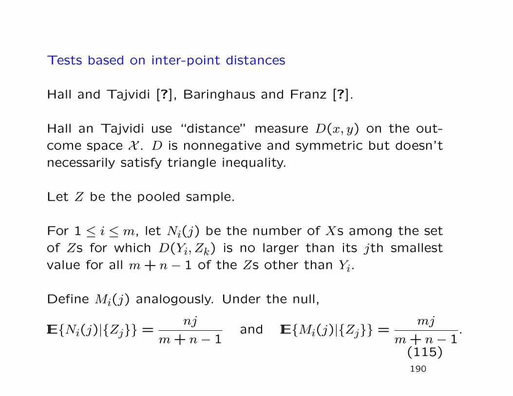
Tests based on inter-point distances
Hall and Tajvidi [?], Baringhaus and Franz [?].
Hall an Tajvidi use “distance” measure D(x, y) on the out-come space X . D is nonnegative and symmetric but doesn’tnecessarily satisfy triangle inequality.
Let Z be the pooled sample.
For 1 ≤ i ≤ m, let Ni(j) be the number of Xs among the setof Zs for which D(Yi, Zk) is no larger than its jth smallestvalue for all m+ n− 1 of the Zs other than Yi.
Define Mi(j) analogously. Under the null,
IENi(j)|Zj =nj
m+ n− 1and IEMi(j)|Zj =
mj
m+ n− 1.
(115)190

Test statistic combines |Mi(j)− IEMi(j)| and |Ni(j)− IENi(j)|,for instance a weighted average of powers of them:
T =1
n
n∑i=1
m∑j=1
|Mi(j)−IEMi(j)|γw1(j)+1
m
m∑i=1
n∑j=1
|Ni(j)−IENi(j)|γw2(j).
(116)
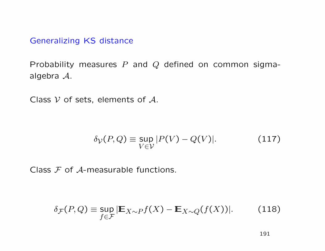
Generalizing KS distance
Probability measures P and Q defined on common sigma-
algebra A.
Class V of sets, elements of A.
δV(P,Q) ≡ supV ∈V|P (V )−Q(V )|. (117)
Class F of A-measurable functions.
δF(P,Q) ≡ supf∈F|IEX∼Pf(X)− IEX∼Q(f(X))|. (118)
191
Special case: F consists of indicator functions of elements of
V.
If X = IR and F is the set of functions with variation bounded
by 1, δF is the KS distance.
192

δ is a pseudo-metric on probability distributions on X
Need to show that it is positive semi-definite and satisfies the
triangle inequality.
Positive semi-definiteness and symmetry are immediate (from
absolute value).
Triangle inequality: For probabilities P,Q, S,
193
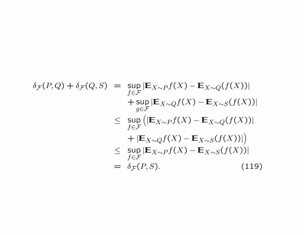
δF(P,Q) + δF(Q,S) = supf∈F|IEX∼Pf(X)− IEX∼Q(f(X))|
+ supg∈F|IEX∼Qf(X)− IEX∼S(f(X))|
≤ supf∈F
(|IEX∼Pf(X)− IEX∼Q(f(X))|
+ |IEX∼Qf(X)− IEX∼S(f(X))|)
≤ supf∈F|IEX∼Pf(X)− IEX∼S(f(X))|
= δF(P, S). (119)
δ is a metric for suitable F
The cone or star of a subset F of a linear vector space is the
set αf : f ∈ F , α ∈ [0,1).
If the cone of F is dense in C(X ) in L∞(X ), then δF is a metric
on probability distributions. (Need to show that δF(P,Q) = 0
iff P = Q.)
(The cone generated by the rational numbers between −1
and 1 is dense in the reals in absolute-value distance, for
example.)
194

Finding δ is easy if F is the unit RKHS ball
In a RKHS H. Let the point-evaluator at x be kx, so f(x) =
〈f, kx〉. The kernel is K(x, y) = 〈kx, ky〉, which is kx viewed as
a function of x and of its argument.
Let
µP ≡ IEX∼PkX = IEX∼PK(X, y). (120)
Then
IEX∼Pf(X) = IEX∼P 〈kx, f〉 = 〈µP , f〉. (121)
(The function f is deterministic; we are averaging its values
when its argument X is drawn at random according to P .)
195

Finding δ, contd. We are taking F = f ∈ H : ‖f‖H ≤ 1.
δF(P,Q) = supf :‖f‖H≤1
|〈µP , f〉 − 〈µQ, f〉|
= supf :‖f‖H≤1
〈µP − µQ, f〉
= ‖µP − µQ‖. (122)
The last step follows from the equivalence of the operator
norm and the Hilbert-space norm, since H is reflexive (self-
dual).
196
Finding δ, contd. Maximizing a continuous function over the
closed unit ball in H:
f∗(y) ≡ arg maxf :‖f‖H≤1
〈µP − µQ, f〉 = (µP − µQ)/‖µP − µQ‖
=IEX∼PK(X, y)− IEX∼QK(X, y)
‖IEX∼PK(X, y)− IEX∼QK(X, y)‖.(123)
The plug-in estimate is
f∗(y) ≡1
n
n∑j=1
K(Xj, y)−1
m
m∑j=1
K(Yj, y). (124)
It is biased, but I’m not convinced that matters.
197

Gretton et al. [?] propose test statistic: Pick F, a set of
functions whose star is dense in C(X ) wrt L∞(X ). They use
the unit ball in a universal RKHS.
Test statistic is a variant of δF(P , Q):
MMD(F , P,Q) = IEX,Y∼PK(X,Y )−2IEX∼P,Y∼QK(X,Y )+IEX,Y∼QK(X,Y ).
(125)
198

They calibrate by bootstrap. Why not calibrate by permuta-
tion?
199
Tests and Confidence Sets for percentiles of a continuous
distribution
Test statistic?
Under what group is the distribution of the the test statistic
invariant if the null is true?
How can we generate the orbit of the data under that group?
How big is the orbit?
How can we sample at random from the orbit?
200

Abstract permutation tests
See old lecture notes, chapter 8.
Earthquake catalog declustering: see PSU talk.
201
Nonparametric Combinations of Tests (NPC)
Setting: multidimensional data, typically mixed types (some
variables continuous, some [possibly ordered] categorical ,
etc.)
Use k > 1 partial tests.
Notation will follow [?]. Have C samples of V -dimensional
data (each sample might correspond to a different treatment,
e.g.). Sample space for each observation is X . Samples may
have unequal sizes.
202
NPC: Notation
Data
X = XjCj=1 = Xjinji=1
Cj=1 = Xhji
nji=1
Cj=1
Vh=1. (126)
n ≡C∑j=1
nj. (127)
For each j, Xjinji=1 are iid Pj ∈ P. Known class P of distri-
butions on a common sigma algebra on X .
Null hypothesis H0: Pj are all equal.
Then have exchangeability w.r.t. C groups.203
NPC: Notation, contd.
H0 might be broken into sub-hypotheses H0iki=1, such that
H0 = ∩ki=1H0i. (128)
H0 is the overall null.
Alternative can be broken into
H1 = ∪ki=1H1k. (129)
H1 is overall alternative.
k-dimensional vector of test statistics T(X)
204
Randomized experiment
There are N subjects.
The subjects are given; they are not necessarily a sample
from some larger population.
Assign a simple random sample of size n of the N subjects to
treatment, and the remaining m = N −n subjects to control.
For each subject, we observe a (univariate) quantitative re-
sponse. (More on multivariate responses later.)
No assumption about the values of that quantitative re-
sponse; they need not follow any particular distribution.
The null hypothesis is that treatment “makes no difference.”205

What’s the relevant group?
Under what group is the distribution of the data invariant if
the null is true?
How can we generate the orbit of the data under that group?
How big is the orbit?
How can we sample at random from the orbit?
206

Alternative hypotheses
Many alternatives are interesting. The most common are the
shift alternative, the dispersion alternative, and the omnibus
alternative.
The shift alternative is that treatment changes the mean
response. (There are left-sided, right-sided and two-sided
versions of the shift alternative.)
The dispersion alternative is that treatment changes the scat-
ter of the responses.
The omnibus alternative is that treatment changes the re-
sponse in some way—any way whatsoever.
207
Testing
The deliberate randomization makes it possible to test rig-
orously whether whether treatment affects response in the
group of N subjects.
Up to sampling error—which can be quantified—differences
between the responses of the treatment and control groups
must be due to the effect of treatment: randomization tends
to balance other factors that affect the responses, and that
otherwise would lead to confounding.
However, conclusions about the effect of treatment among
the N subjects cannot be extrapolated to any other popula-
tion, because we do not know where the subjects came from
(how they came to be part of the experiment).
208
The Neyman Model
We model the experiment as follows: Each of the N subjectsis represented by a ticket with two numbers on it, a left anda right number.
The left number is the response the subject would have if as-signed to the control group; the right number is the responsethe subject would have if assigned to the treatment group.
These numbers are written on the tickets before the exper-iment starts. Assigning the subject to treatment or controlonly determines whether we observe the left or the right num-ber for that subject.
Let uj be the left number on the jth ticket and let vj be theright number on the jth ticket.
The experiment reveals either uj (if subject j is assigned totreatment) or vj (if subject j is assigned to control).
209
Non-interference
There are only two numbers on each ticket.
Whether uj or vj is revealed depends only on whether subjectj is assigned to treatment or to control.
Let Xj be the indicator of whether subject j was treated.That is, Xj = 0 if subject j is in the control group, andXj = 1 if subject j is in the treatment group.
If Xj = 0, uj is revealed. If Xj = 1, vj is revealed.
More generally, the observed response of subject j could de-pend on all the assignments Xjnj=1.
In the Neyman model, it depends only on Xj. This is thehypothesis of non-interference.
210
Strong Null Hypotheses
The strong null hypothesis is
uj = vj, j = 1,2, . . . , N. (130)
That is, the strong null hypothesis is that the left and right
numbers on each ticket are equal. Subject by subject, treat-
ment makes no difference at all. The N observed responses
will be the same, no matter which subjects are assigned to
treatment.
211
Weak Null Hypotheses
The weak null hypothesis is that the average of the left num-
bers equals the average of the right numbers:
N∑j=1
uj =N∑j=1
vj. (131)
In the weak null hypothesis, treatment makes no difference
on average: treatment might increase the responses for some
individuals, provided it decreases the responses of other indi-
viduals by a balancing amount.
212
Extending the Neyman Model to random responses
Generalize ticket model from two responses (one under treat-
ment, the other under control) to two random variables.
Instead of thinking of subject j’s (potential) responses as a
fixed pair of numbers (uj, vj)Nj=1, think of them as a pair
of random variables (Uj, Vj).
A realization of Uj will be observed if subject j is assigned to
control (i.e., if Xj = 0)
A realization of Vj will be observed if subject j is assigned to
treatment (i.e., if Xj = 1)
The joint probability distributions of Uj and Vj are fixed before
the randomization (but are unknown).213

Assumption of no confounding
Xj are in general dependent (e.g., if m subjects are selected
for treatment at random).
But Xj don’t depend on characteristics of the subjects (in-
cluding (Uj, Vj)).
The set Xjnj=1 is independent of the set (Uj, Vj)nj=1.
214
Assumption of Non-Interference
The random pairs
(Uj, Vj)Nj=1 (132)
are independent across j. That is, if we knew the values of
any subset of the pairs, it wouldn’t tell us anything about the
values of the rest of the pairs.
(Within each pair, Uj and Vj can be dependent.)
Nothing about subject j’s potential responses depends on any
other subjects.
215
Fine points
Think of the realizations of (Uj, Vj) as being generated
before Xj are generated.
Once (Uj, Vj) are generated, they are intrinsic properties of
subject j.
216
Null hypotheses
• For each j, Uj ∼ Vj
• For each j, IEUj = IEVj
• IE∑Nj=1Uj = IE
∑Nj=1 Vj
• qth quantile of Uj equals qth quantile of Vj (e.g., for
survival time)
• what else?
217

Special case: Binary responses
die, live, don’t improve, improve, not harmed, harmed.
Code responses as 0, 1.
Then subject j is characterized by 4 numbers that specify
joint distribution of (Uj, Vj).
pj = PrUj = 0 and Vj = 0qj = PrUj = 0 and Vj = 1rj = PrUj = 1 and Vj = 0sj = PrUj = 1 and Vj = 1 (133)
pj, qj, rj, sj ≥ 0 and pj + qj + rj + sj = 1.
218
Causal inference
Think of treatment as exposure to something that might
cause harm (e.g., a potential carcinogen).
A response of 1 means the subject was “harmed” (e.g., got
cancer). A response of 0 means the subject was not harmed.
E.g., if Xj = 1 and Vj = 1, subject j was exposed and suffered
harm. If Xj = 0 and Uj = 1, subject j was not exposed, but
suffered harm.
In general, does exposure cause harm?
Would exposure cause harm to subject j?
If Xj = 1 and Vj = 1, did exposure harm subject j?
219
Relative risk
Generally, data are from epidemiological studies, not random-ized experiments: confounding is a major concern.
Pretend we have controlled, randomized, double-blind exper-iment.
Recall that n =∑jXj is the number of exposed (treated)
subjects and m = N − n =∑j(1 − Xj) is the number of
unexposed (control) subjects.
Common test for causation is based on relative risk (RR):
RR =1n
∑XjVj
1m
∑(1−Xj)Uj
. (134)
Numerator is the rate of harm in the treated group; denom-inator is the rate of harm in the control group.
220
General and specific causation in the law
Plaintiff was exposed to something, was harmed, and sues
the party responsible for his exposure.
To win, plaintiff must show by a preponderance of the evi-
dence (i.e., that more likely than not):
General causation: exposure can cause harm
Specific causation: the exposure caused that individual’s
harm
221
Relative risk and specific causation
Common legal test for specific causation: RR > 2.
Claim: if RR > 2, “more likely than not” the exposure caused
plaintiff’s harm.
222
Thought experiment
2000 subjects. 1000 subjects selected at random and ex-
posed; 1000 left unexposed.
Among unexposed, 2 are harmed. Among exposed, 20 are
harmed. Then RR = 10.
Heuristic argument: but for the exposure, there would only
have been 2 harmed among the exposed, so 18 of the 20 in-
juries were caused by the exposure.
223
Is the plaintiff selected at random?
Pick a subject at random from the 20 who were exposed and
harmed.
Pr that subject’s harm was caused by exposure = 18/20
= 90%
= 1−1
RR> 50%.
If the RR had been 4, the chance would have been 75%.
If RR had been 2, the chance would have been 50%: the
threshold for “more likely than not.”
224
Hypothetical Counterfactuals and Causation
Suppose Xj = 1 and Vj = 1 (subject j was exposed and
harmed).
Exposure caused the harm if Uj = 0: But for the exposure,
subject j would not have been harmed.
Involves counterfactual: Subject j was in fact exposed!
(If Uj = 1, subject would have been harmed whether or not
the exposure happened: The exposure did not cause the
harm.)
225

Probability that exposure causes harm
Chance subject j would be harmed if unexposed
βj = PrUj = 1 = rj + sj. (135)
Chance subject j would be harmed if exposed
γj = PrVj = 1 = qj + sj. (136)
βj and γj are identifiable, but (pj, qj, rj, sj) are not separately
identifiable.
Even if βj and γj are known, cannot determine qj.
226

Overall rate of harm caused by exposure
Overall expected rate of harm if no subjects were exposed
β =1
N
N∑j=1
PrUj = 1 =1
N
N∑j=1
(rj + sj). (137)
Overall expected rate of harm if all subjects were exposed
γ =1
N
N∑j=1
PrVj = 1 =1
N
N∑j=1
(qj + sj). (138)
Difference in expected rate of harm if all were exposed versus
if none were exposed
γ − β. (139)
This is average causal effect of exposure on harm (among
the N subjects in the study group).227
Estimating rate of harm caused by exposure
γ, β, γ − β are estimable:
γ = IE1
n
N∑j=1
XjVj (140)
β =1
m
N∑j=1
(1−Xj)Uj. (141)
228

Focus on the algebra, not the statistics
Take γ and β to be known, with
0 < β < γ (142)
(so exposure does, on average, cause harm: RR = γ/β > 1)
and
β + γ < 1 (143)
(the rate of harm, even with exposure, is not too large).
229
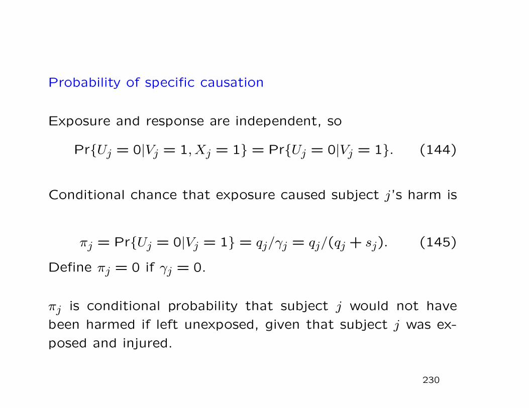
Probability of specific causation
Exposure and response are independent, so
PrUj = 0|Vj = 1, Xj = 1 = PrUj = 0|Vj = 1. (144)
Conditional chance that exposure caused subject j’s harm is
πj = PrUj = 0|Vj = 1 = qj/γj = qj/(qj + sj). (145)
Define πj = 0 if γj = 0.
πj is conditional probability that subject j would not have
been harmed if left unexposed, given that subject j was ex-
posed and injured.
230
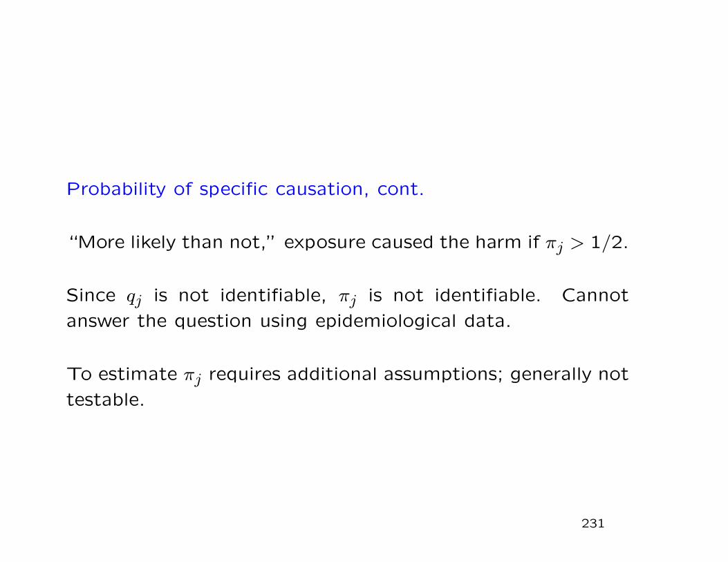
Probability of specific causation, cont.
“More likely than not,” exposure caused the harm if πj > 1/2.
Since qj is not identifiable, πj is not identifiable. Cannot
answer the question using epidemiological data.
To estimate πj requires additional assumptions; generally not
testable.
231
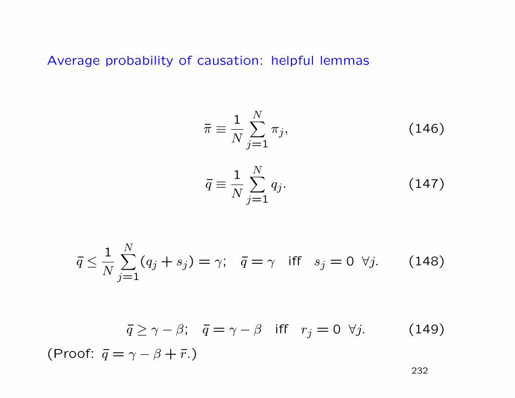
Average probability of causation: helpful lemmas
π ≡1
N
N∑j=1
πj, (146)
q ≡1
N
N∑j=1
qj. (147)
q ≤1
N
N∑j=1
(qj + sj) = γ; q = γ iff sj = 0 ∀j. (148)
q ≥ γ − β; q = γ − β iff rj = 0 ∀j. (149)
(Proof: q = γ − β + r.)232

Average probability of causation: lower bound
inf π = γ − β. (150)
Proof.
π =1
N
N∑j=1
πj ≥1
N
N∑j=1
(qj + sj)πj =1
N
N∑j=1
qj = q ≥ γ − β.
(151)
Equality holds if rj = 0 for all subjects, and qj = 0 unless
qj + sj = 1.
For instance, suppose there are two types of subjects: for one
type, exposure does not change the chance of harm, while
for the other, there is harm only if the subject is exposed.
233
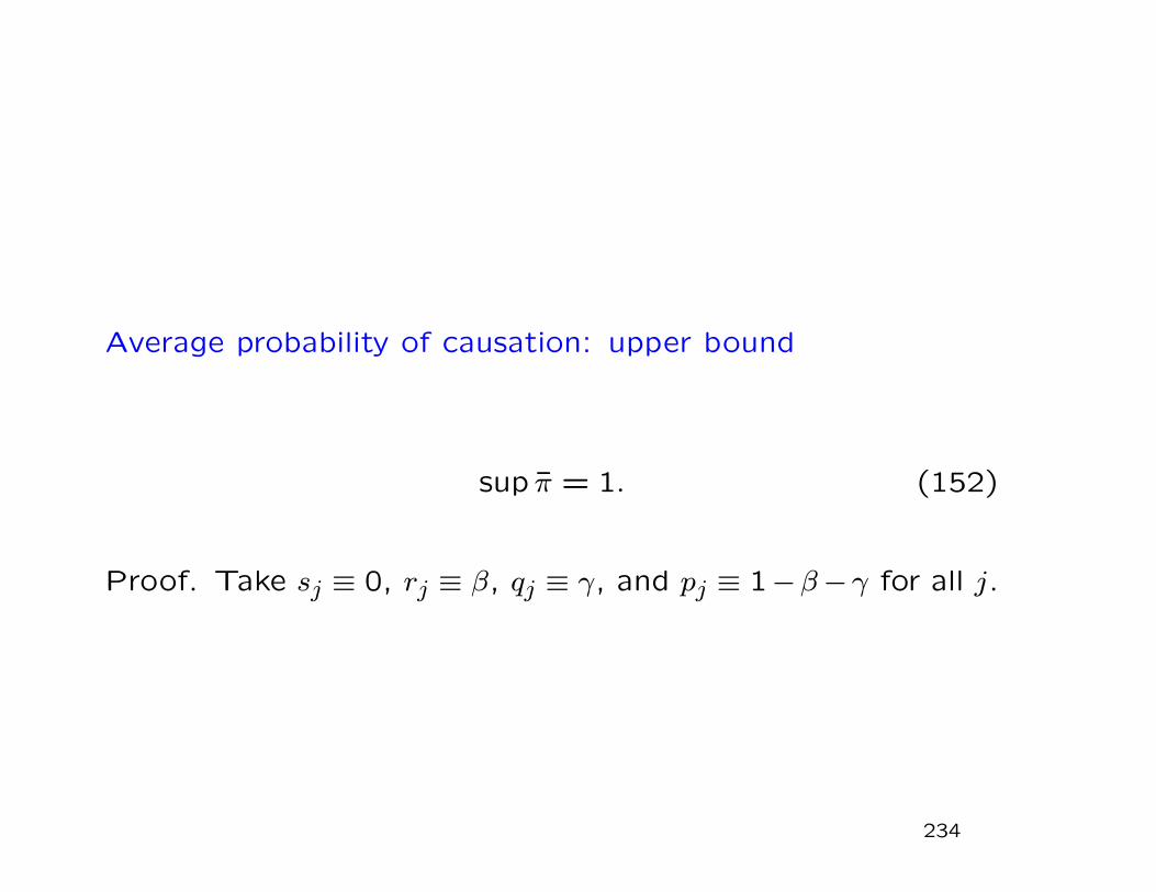
Average probability of causation: upper bound
sup π = 1. (152)
Proof. Take sj ≡ 0, rj ≡ β, qj ≡ γ, and pj ≡ 1−β−γ for all j.
234

Example: πj = π = 1
pj = 0.95, qj = 0.04, rj = 0.01, sj = 0. Then
πj = qj/(qj + sj) = 0.04/(0.04 + 0) = 1, ∀j. (153)
Note that
β = r + s = 0.01 < q + s = γ = 0.04 (154)
and β + γ = 0.05 < 1.
235
Example: πj = π = 3/4
pj = 0.96, qj = 0.03, rj = 0, sj = 0.01. Then
πj = qj/(qj + sj) = 0.03/(0.03 + 0.01) = 3/4, ∀j. (155)
Note that
β = r + s = 0.01 < q + s = γ = 0.04 (156)
and β + γ = 0.05 < 1.
236
Example: πj = π = 0.03
For 97% of subjects, pj = 96/97, qj = rj = 0, sj = 1/97.
For 3% of subjects, pj = 0, qj = 1, rj = sj = 0.
For the first group,
πj = qj/(qj + sj) = 0/(0 + 1/97) = 0. (157)
For the second group,
πj = qj/(qj + sj) = 1/(1 + 0) = 1. (158)
Hence
π = 0.97× 0 + 0.03× 1 = 0.03. (159)
Again β = 0.01, γ = 0.04.
All three examples have the same values of p, q, r, and s—and hence of β and γ—but the values of π are 1, 3/4, and0.03.
237

Epidemiological studies can (at best) determine β and γ.
The claim that RR > 2 means causation is “more likely than
not” ties to example 2.
238
Probability of specific causation: random selection
Plaintiff was exposed and harmed. What is the chance that
exposure caused the harm?
Arguments generally assume plaintiff was chosen at random
from the study group. But how?
1. Pick subject at random; condition that subject was ex-
posed and harmed.
2. Divide subjects into 2 groups, exposed and not. Condition
that at least one exposed was harmed. Pick one subject at
random from the exposed and harmed.
3. Pick a subject at random; condition that subject was ex-
posed and harmed and that subject sues.239
In all three, n of N are assigned at random to exposure,
exposure Xj is independent of response pair (Uj, Vj), and
(Uj, Vj)Nj=1 are independent random pairs.

Probability of specific causation: scenario 1
η is a random integer between 1 and N . Condition that
Xη = Vη = 1.
Then
PrUη = 0|Xη = 1, Vη = 1 ≥ 1−1
RR. (160)
Can be as high as 1.
240
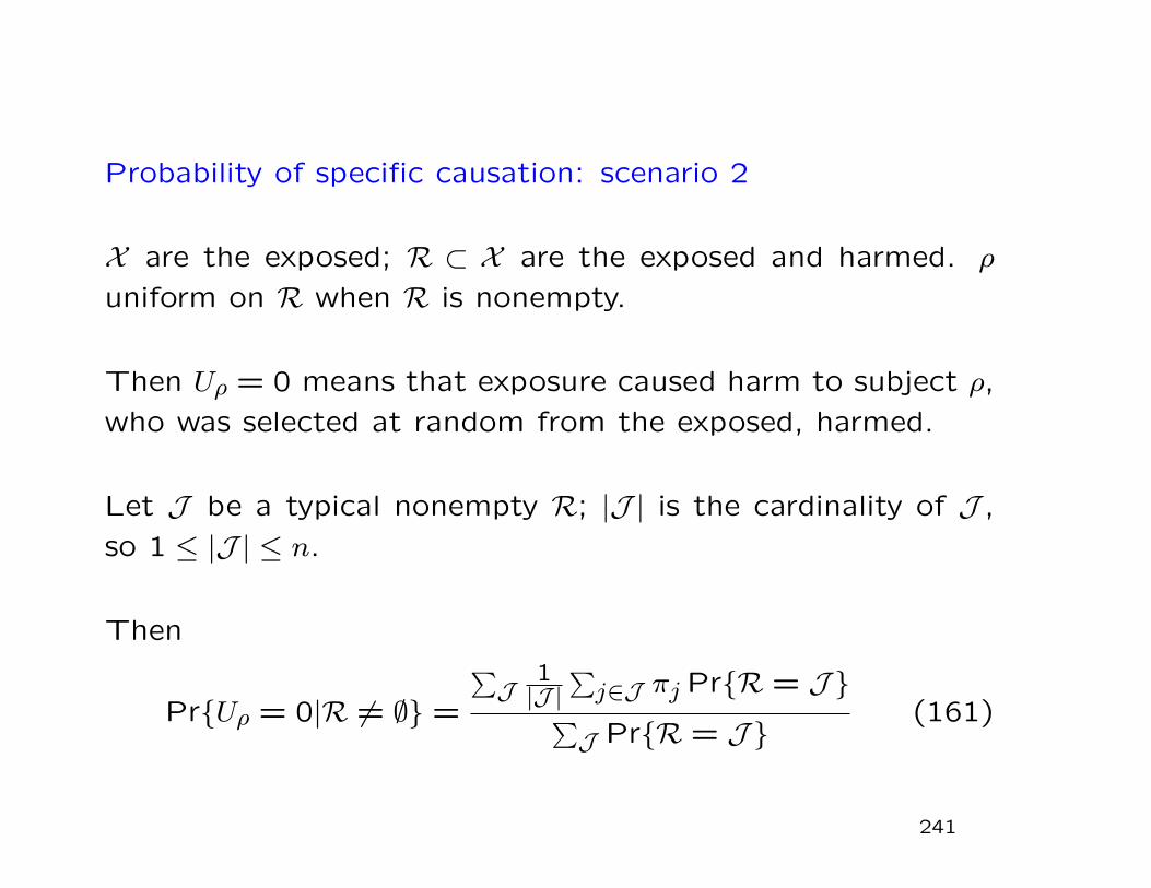
Probability of specific causation: scenario 2
X are the exposed; R ⊂ X are the exposed and harmed. ρ
uniform on R when R is nonempty.
Then Uρ = 0 means that exposure caused harm to subject ρ,
who was selected at random from the exposed, harmed.
Let J be a typical nonempty R; |J | is the cardinality of J ,
so 1 ≤ |J | ≤ n.
Then
PrUρ = 0|R 6= ∅ =
∑J
1|J |
∑j∈J πj PrR = J∑J PrR = J
(161)
241
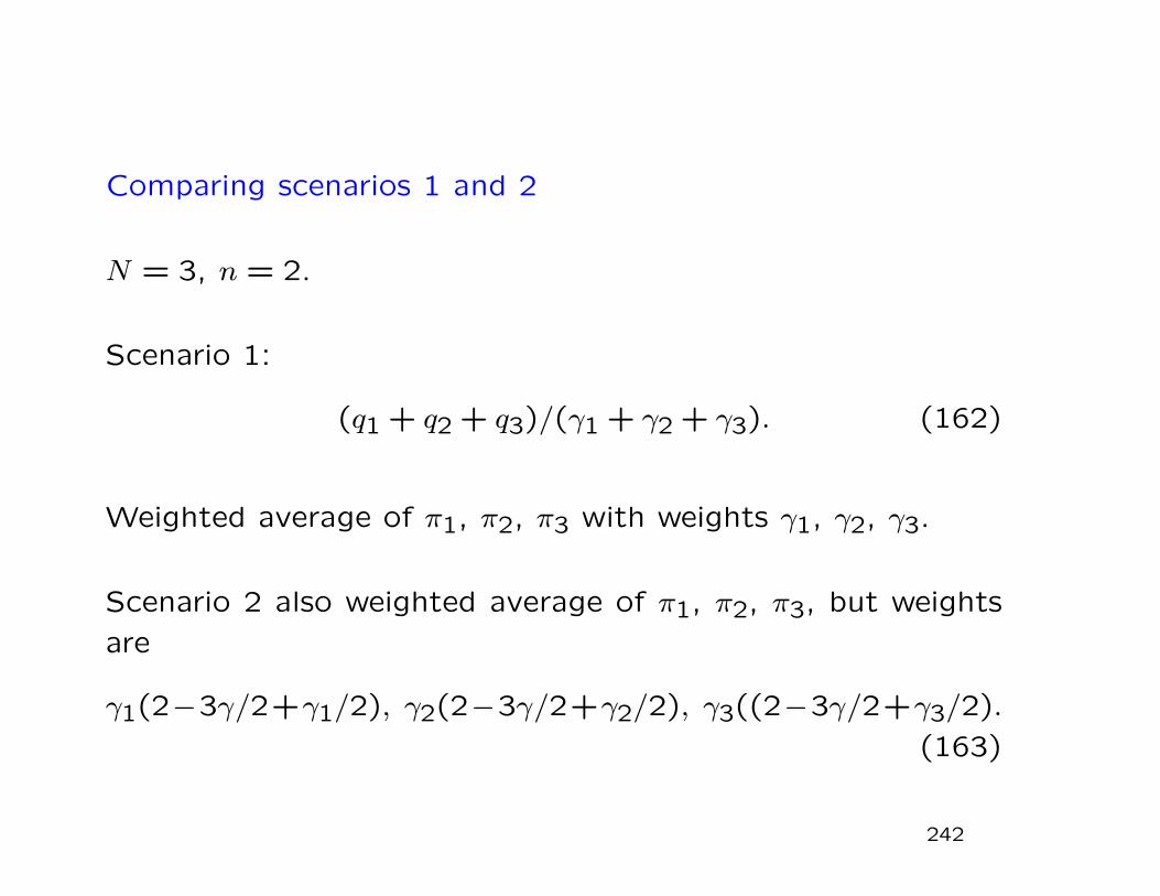
Comparing scenarios 1 and 2
N = 3, n = 2.
Scenario 1:
(q1 + q2 + q3)/(γ1 + γ2 + γ3). (162)
Weighted average of π1, π2, π3 with weights γ1, γ2, γ3.
Scenario 2 also weighted average of π1, π2, π3, but weights
are
γ1(2−3γ/2+γ1/2), γ2(2−3γ/2+γ2/2), γ3((2−3γ/2+γ3/2).
(163)
242
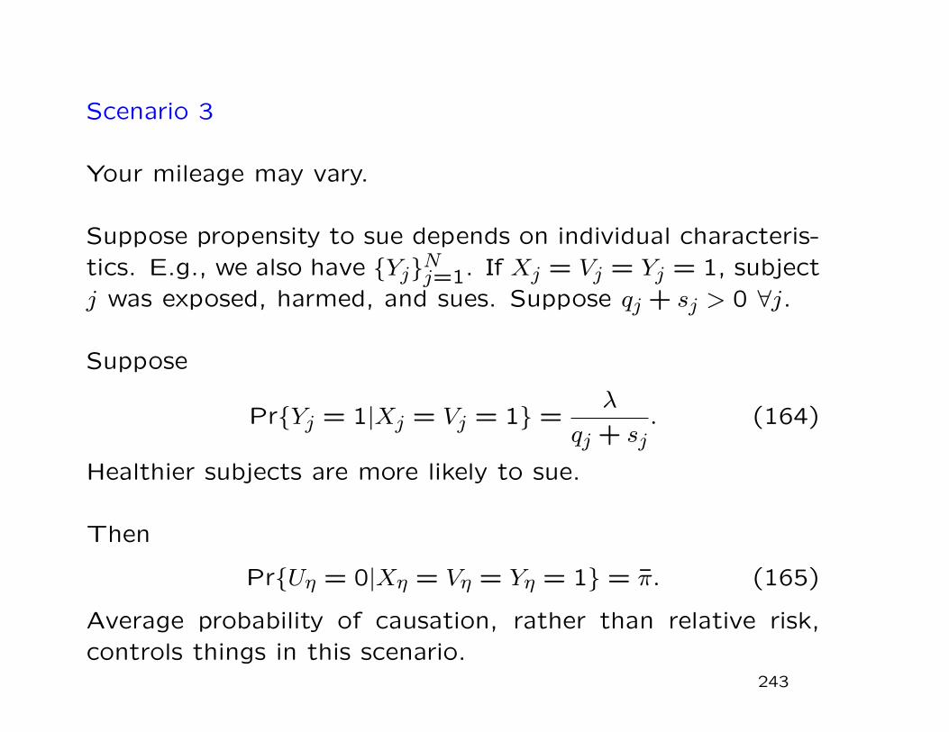
Scenario 3
Your mileage may vary.
Suppose propensity to sue depends on individual characteris-tics. E.g., we also have YjNj=1. If Xj = Vj = Yj = 1, subjectj was exposed, harmed, and sues. Suppose qj + sj > 0 ∀j.
Suppose
PrYj = 1|Xj = Vj = 1 =λ
qj + sj. (164)
Healthier subjects are more likely to sue.
Then
PrUη = 0|Xη = Vη = Yη = 1 = π. (165)
Average probability of causation, rather than relative risk,controls things in this scenario.
243

Bibliography
244

10
E.L. Bennett, M.R. Rosenzweig, and M.C. Diamond. Ratbrain: Effects of environmental enrichment on wet and dryweights. Science, 163:825–826, 1969.
D. Freedman, R. Pisani, R. Purves, and A. Adhikari. Statis-tics. W.W. Norton and Co., New York, 4th edition, 2004.
D.A. Freedman and P.B. Stark. The swine flu vaccine andGuillain-Barre syndrome: a case study in relative risk andspecific causation. Evaluation Review, 23:619–647, 1999.
E.L. Lehmann. Testing Statistical Hypotheses. Springer,New York, 3rd edition, 2005.
E.L. Lehmann and G. Casella. Theory of Point Estimation.Springer-Verlag, New York, 2nd edition, 1998.
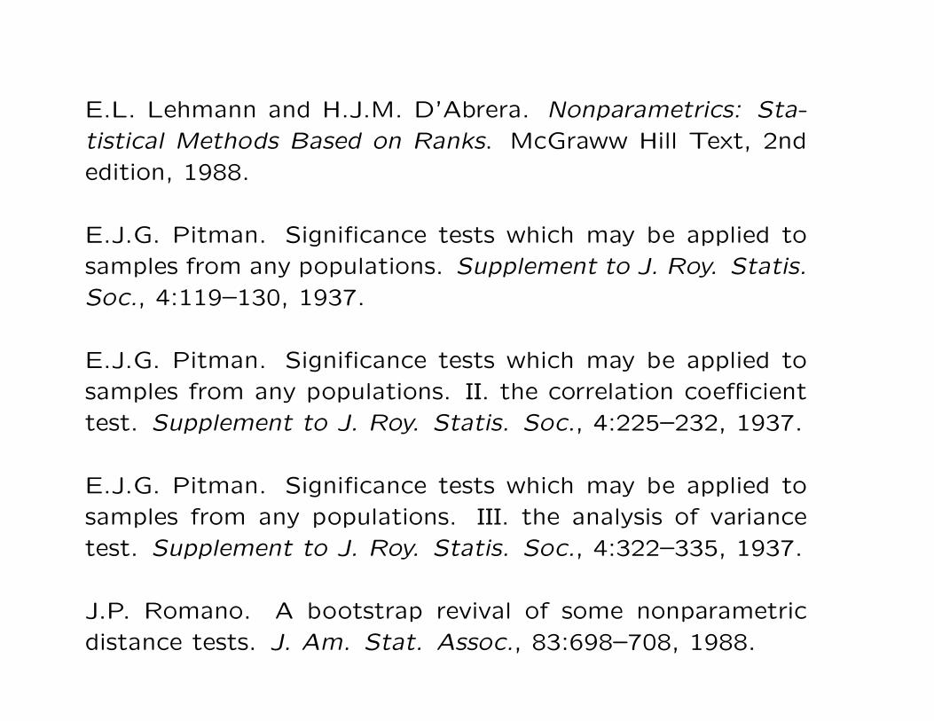
E.L. Lehmann and H.J.M. D’Abrera. Nonparametrics: Sta-tistical Methods Based on Ranks. McGraww Hill Text, 2ndedition, 1988.
E.J.G. Pitman. Significance tests which may be applied tosamples from any populations. Supplement to J. Roy. Statis.Soc., 4:119–130, 1937.
E.J.G. Pitman. Significance tests which may be applied tosamples from any populations. II. the correlation coefficienttest. Supplement to J. Roy. Statis. Soc., 4:225–232, 1937.
E.J.G. Pitman. Significance tests which may be applied tosamples from any populations. III. the analysis of variancetest. Supplement to J. Roy. Statis. Soc., 4:322–335, 1937.
J.P. Romano. A bootstrap revival of some nonparametricdistance tests. J. Am. Stat. Assoc., 83:698–708, 1988.
J.P. Romano. On the behavior of randomization tests with-
out a group invariance assumption. J. Am. Stat. Assoc.,
85:686–692, 1990.
M.R. Rosenzweig, E.L. Bennett, and M.C. Diamond. Brain
changes in response to experience. Scientific American, 226:22–
29, 1972.