advanced statistics-19 |nonparametric regression ii
TRANSCRIPT
Advanced Statistics-19—Nonparametric regression II
Changliang Zou
Institute of Statistics, Nankai University
Email: [email protected]
Changliang Zou Advanced Statistics-19, Spring 2021
Uniform convergence
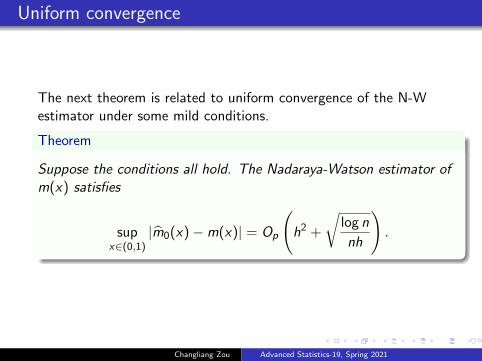
The next theorem is related to uniform convergence of the N-Westimator under some mild conditions.
Theorem
Suppose the conditions all hold. The Nadaraya-Watson estimator ofm(x) satisfies
supx∈(0,1)
|m̂0(x)−m(x)| = Op
(h2 +
√log n
nh
).
Changliang Zou Advanced Statistics-19, Spring 2021

Uniform convergence
The study on uniform convergence of various nonparametricestimators has a long history; see Silverman (1978) for example.
In this part, we will impose certain stringent conditions on themoments of ε and bandwidth so that a simple proof of thistheorem is achievable.
Changliang Zou Advanced Statistics-19, Spring 2021

Uniform convergence
Additional conditions
Assumption (Density of x)
The density of the i.i.d. xi ’s, f (x), is bounded away from zero on thecompact support (0, 1).
Assumption (Moments condition)
For a fixed C <∞, E(|εi |θ) ≤ C <∞.
Assumption (Kernel and bandwidth condition)
The h satisfies n1/θ/√
nh→ 0 as n→∞; K (·) is a Lipschitzcontinuous function.
Changliang Zou Advanced Statistics-19, Spring 2021

Proof: preliminaries
Lemma (Bernstein’s inequality)
Let X1, . . . ,Xn be independent centered random variables a.s.bounded by A <∞ in absolute value. Let σ2 = n−1
∑ni=1 E (X 2
i ).Then for all x > 0,
Pr( n∑
i=1
Xi ≥ x)≤ exp
(− x2
2nσ2 + 2Ax/3
).
Lemma
Suppose the conditions in theorem hold. We have,
supx∈(0,1)
∣∣∣f̂h(x)− f (x)∣∣∣ = Op
(h2 +
√log n
nh
).
Changliang Zou Advanced Statistics-19, Spring 2021

Proof: preliminaries
Denote bn =√
log nnh and εi = σ(xi )εi
The m̂0(x) can be expressed as
m̂0(x) =1
nf̂h(x)
n∑i=1
Kh(xi − x)m(xi ) +1
nf̂h(x)
n∑i=1
Kh(xi − x)εi
=:A1(x)
f̂h(x)+
A2(x)
f̂h(x).
By Lemma 2, we have
supx|A1(x)/f̂h(x)−m(x)| = Op(h2 + bn).
Thus, it remains to show that supx |A2(x)| = Op(bn).
Changliang Zou Advanced Statistics-19, Spring 2021

Proof: preliminaries
We truncate the error εi by a quantity ψn = n1/(θ−δ), for some smallpositive number δ > 0. Moreover, define
ε≤i = εi I(|εi | ≤ ψn) and ε>i = εi I(|εi | > ψn).
Accordingly, A2(x) can be rewritten as
A2(x) = n−1n∑
i=1
Kh(xi − x)ε≤i + n−1n∑
i=1
Kh(xi − x)ε>i
:= n−1n∑
i=1
Z≤i (x) + n−1n∑
i=1
Z>i (x) (1)
Changliang Zou Advanced Statistics-19, Spring 2021
Proof: main
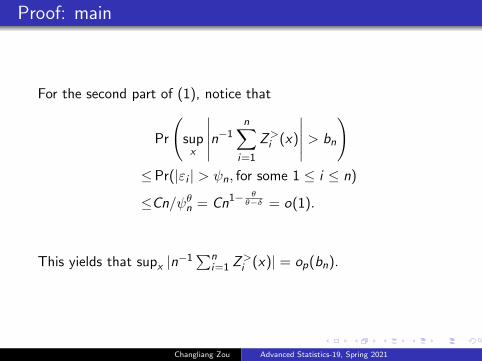
For the second part of (1), notice that
Pr
(supx
∣∣∣∣∣n−1n∑
i=1
Z>i (x)
∣∣∣∣∣ > bn
)≤Pr(|εi | > ψn, for some 1 ≤ i ≤ n)
≤Cn/ψθn = Cn1− θθ−δ = o(1).
This yields that supx |n−1∑n
i=1 Z>i (x)| = op(bn).
Changliang Zou Advanced Statistics-19, Spring 2021
Proof: main
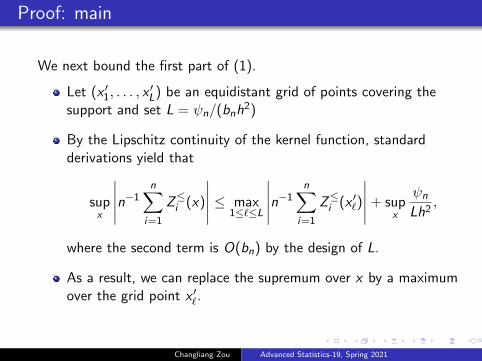
We next bound the first part of (1).
Let (x ′1, . . . , x′L) be an equidistant grid of points covering the
support and set L = ψn/(bnh2)
By the Lipschitz continuity of the kernel function, standardderivations yield that
supx
∣∣∣∣∣n−1n∑
i=1
Z≤i (x)
∣∣∣∣∣ ≤ max1≤`≤L
∣∣∣∣∣n−1n∑
i=1
Z≤i (x ′`)
∣∣∣∣∣+ supx
ψn
Lh2,
where the second term is O(bn) by the design of L.
As a result, we can replace the supremum over x by a maximumover the grid point x ′`.
Changliang Zou Advanced Statistics-19, Spring 2021
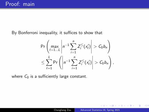
Proof: main
By Bonferroni inequality, it suffices to show that
Pr
(max`=1...L
∣∣∣∣∣n−1n∑
i=1
Z≤i (x ′`)
∣∣∣∣∣ > C0bn
)
≤L∑`=1
Pr
(∣∣∣∣∣n−1n∑
i=1
Z≤i (x ′`)
∣∣∣∣∣ > C0bn
),
where C0 is a sufficiently large constant.
Changliang Zou Advanced Statistics-19, Spring 2021
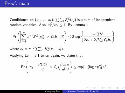
Proof: main
Conditioned on (x1, . . . , xp),∑n
i=1 Z≤i (x ′`) is a sum of independent
random variables. Also, ε≤i /ψn ≤ 1. By Lemma 1
Pr
(∣∣∣∣∣n∑
i=1
n−1Z≤i (x ′`)
∣∣∣∣∣ > C0bn | X
)≤ 2 exp
{−C 2
0 b2n
2cn + 2/3ψn
nhC0bn
},
where cn = n−2∑n
i=1 K 2h (xi − x ′`).
Applying Lemma 1 to cK again, we claim that
Pr
{∣∣∣∣cn − R(K )
nh
∣∣∣∣ > C0
√log n
n3h3
}≤ exp{−(log n)C 2
0 /2}
Changliang Zou Advanced Statistics-19, Spring 2021
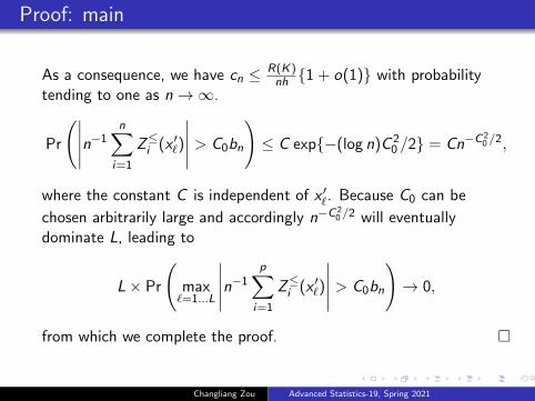
Proof: main
As a consequence, we have cn ≤ R(K)nh {1 + o(1)} with probability
tending to one as n→∞.
Pr
(∣∣∣∣∣n−1n∑
i=1
Z≤i (x ′`)
∣∣∣∣∣ > C0bn
)≤ C exp{−(log n)C 2
0 /2} = Cn−C20 /2,
where the constant C is independent of x ′`. Because C0 can be
chosen arbitrarily large and accordingly n−C20 /2 will eventually
dominate L, leading to
L× Pr
(max`=1...L
∣∣∣∣∣n−1p∑
i=1
Z≤i (x ′`)
∣∣∣∣∣ > C0bn
)→ 0,
from which we complete the proof. �
Changliang Zou Advanced Statistics-19, Spring 2021
Other smoothers
Orthogonal series regression
Polynomial spline
Smoothing spline
Changliang Zou Advanced Statistics-19, Spring 2021
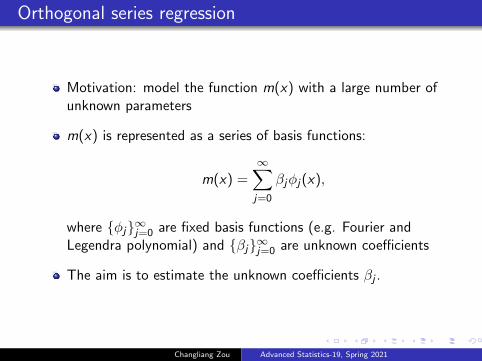
Orthogonal series regression
Motivation: model the function m(x) with a large number ofunknown parameters
m(x) is represented as a series of basis functions:
m(x) =∞∑j=0
βjφj(x),
where {φj}∞j=0 are fixed basis functions (e.g. Fourier andLegendra polynomial) and {βj}∞j=0 are unknown coefficients
The aim is to estimate the unknown coefficients βj .
Changliang Zou Advanced Statistics-19, Spring 2021
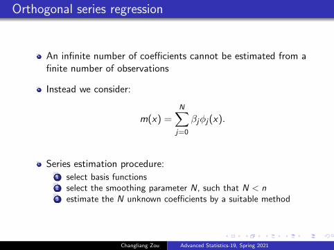
Orthogonal series regression
An infinite number of coefficients cannot be estimated from afinite number of observations
Instead we consider:
m(x) =N∑j=0
βjφj(x).
Series estimation procedure:1 select basis functions2 select the smoothing parameter N, such that N < n3 estimate the N unknown coefficients by a suitable method
Changliang Zou Advanced Statistics-19, Spring 2021
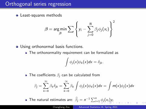
Orthogonal series regression
Least-squares methods
β = arg minβ
∑yi −N∑j=0
βjφj(xi )
2
Using orthonormal basis functions.
The orthonormality requirement can be formalized as∫φj(x)φk(x)dx = δjk .
The coefficients βj can be calculated from
βj =∞∑k=0
βkδjk =∞∑k=0
βk
∫φj(x)φk(x)dx =
∫m(x)φj(x)dx
The natural estimates are: β̂j = n−1∑n
i=1 φj(xi )yi
Changliang Zou Advanced Statistics-19, Spring 2021

Polynomial Spline: idea
Recall that we are interested in the conditional expectationfunction of Y given X , m(x) = E (Y | X = x)
By Taylor expansion, we can approximate m(x) byg(x) = a0 + a1x + · · ·+ akxk
Polynomial splines approximate the function piecewise
Partition the region of x into several subintervals by t1, . . . , tJ , asequence of fixed points such that
−∞ < t1 < t2 < · · · < tJ <∞
{t1, . . . , tJ} are called knots.
Changliang Zou Advanced Statistics-19, Spring 2021
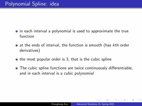
Polynomial Spline: idea
in each interval a polynomial is used to approximate the truefunction
at the ends of interval, the function is smooth (has kth orderderivatives)
the most popular order is 3, that is the cubic spline
The cubic spline functions are twice continuously differentiable,and in each interval is a cubic polynomial
Changliang Zou Advanced Statistics-19, Spring 2021

Cubic spline: power basis
B1(x) = 1,B2(x) = x ,B3(x) = x2,B4(x) = x3,B4+j(x) =(x − tj)
3+, j = 1, . . . , J
A cubic spline function with J knots is given by
s(x) =J+4∑k=1
θkBk(x),
where Bk(x) is the kth spline basis function.
B-splines.
Changliang Zou Advanced Statistics-19, Spring 2021
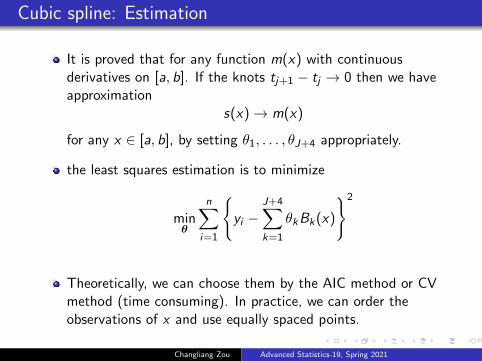
Cubic spline: Estimation
It is proved that for any function m(x) with continuousderivatives on [a, b]. If the knots tj+1 − tj → 0 then we haveapproximation
s(x)→ m(x)
for any x ∈ [a, b], by setting θ1, . . . , θJ+4 appropriately.
the least squares estimation is to minimize
minθ
n∑i=1
{yi −
J+4∑k=1
θkBk(x)
}2
Theoretically, we can choose them by the AIC method or CVmethod (time consuming). In practice, we can order theobservations of x and use equally spaced points.
Changliang Zou Advanced Statistics-19, Spring 2021
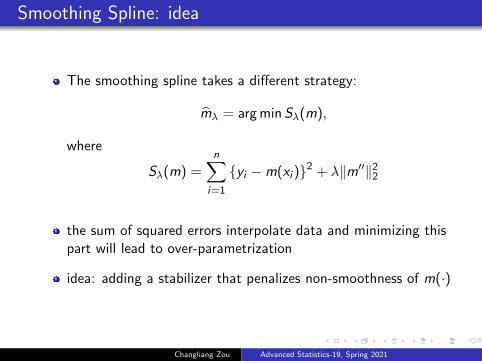
Smoothing Spline: idea
The smoothing spline takes a different strategy:
m̂λ = arg min Sλ(m),
where
Sλ(m) =n∑
i=1
{yi −m(xi )}2 + λ‖m′′‖22
the sum of squared errors interpolate data and minimizing thispart will lead to over-parametrization
idea: adding a stabilizer that penalizes non-smoothness of m(·)
Changliang Zou Advanced Statistics-19, Spring 2021

Smoothing Spline: idea
smoothing parameter λ ≥ 0. For λ = 0, m̂λ interpolates dataand for λ = 1, m̂λ reduces to a linear model.
The (unique) minimizer of Sλ(m) is given by the cubic spline onthe interval [X(1),X(n)]
Changliang Zou Advanced Statistics-19, Spring 2021