stats 20x workshops - aucklandleila/booklet.pdf · 9 test and examination skills ... 9 tutorial...

STUDENT LEARNING CENTRE 3rd Floor

Information Commons

© Student Learning Centre The University of Auckland 1

STATS 20X WORKSHOPS

SEMESTER 1, 2005

Students MUST REGISTER for both workshops with The Student Learning Centre


Information Commons


STUDENT LEARNING CENTRE

Topics we teach and can provide advice on include:

Essay writing Computer skills Reading and note-taking Memory and concentration Report writing Test and examination skills Thesis and dissertation writing Tutorial skills Research skills Time and stress management Mathematics Oral presentation and seminar skills Language learning Specific learning disabilities Motivation and goal setting Survival skills (in the University system)

Programmes within SLC include:

• Te Puni Wananga Maori university tutors committed to enhancing Maori students’ success

• Fale Pasifika

Pacific Island tutors committed to enhancing success for Pacific Island students

• Language Exchange (LEX)

Learn a new language, make a new friend

• English Conversation Groups Improve English, develop critical thinking, and express ideas and opinions.


Information Commons


The Student Learning Centre (SLC) offers help for STATS 20x by offering:

• one-on-one tutoring help, and

• two workshops on stage one revision

One-on-one help

The SLC employs tutors specifically to help students with one-on-one assistance for the Statistics 20x paper. One-on-one tutoring must be booked in at SLC reception.

In Semester 1, 2005 one-on-one tutor help will be offered by:

• Leila Boyle

• Jessica Liang

• Christine Liu

There are no fixed times tutors are available, call the Student Learning Centre to make an appointment.

Note: SLC tutors are not allowed to help students complete their assignments.

SLC Statistics 20x Workshops

Any questions regarding STATS 20x workshops should be forwarded to:

Leila Boyle SLC Statistics Co-ordinator

Email: [email protected]

Workshops are run in a relaxed environment, typically set at a pace for those students that find the statistics department’s tutorials too fast. All workshops allow plenty of time for questions.

In fact, this is encouraged ☺


Information Commons


Saturday Workshops

Include two 4-hour workshops held on Saturday mornings at the beginning of the semester that will help students with stage one revision.

Useful Websites

Link to SLC webpage: http://www.slc.auckland.ac.nz/ug/

Link to Cecil: https://cecil.auckland.ac.nz/

Stage 1 Text Book

Wild, Christopher J. & Seber, George A. F. 2000. Chance Encounters: A First Course in Data Analysis and Inference. John Wiley & Sons, Inc. New York


Information Commons


SECTION ONE POPULATIONS, SAMPLES & CENTRAL LIMIT THEOREM

STUDENT LEARNING CENTRE 3rd Floor Information Commons


WHAT IS STATISTICS

“the need to find out about the world and how it operates… by extracting meaningful patterns from the variation that is everywhere”1

“Statistics is a process of finding out more about the real world”

1 Wild, C.J., Seber, A.F.S. 2000. Chance Encounters: A first course in data analysis and inference. John Wiley & Sons, Inc. New York. p.28

Ways of analysing data (making inferences/statements about unknown parameters)

Chapter 10 • 1-sample t-test • paired t-test • 2-sample t-test • ANOVA / F-test

Chapter 11 Chi-Square tests • Goodness of Fit • Independence • Homogeneity

Chapter 12 Regression • Simple linear model

How to analyse data (the process of analyzing data)

1. Identify population of interest (C1) 2. Select parameter of interest (C7) 3. Determine the best way to analyse - i.e. the best type of Significance test to use

(C9-12) 4. Design the type of study and data collection methods (C1) 5. Collect data and generate summary statistics and plots to make generalizations

about the data (C2-3) 6. Conduct the specified Significance test:

a. Check assumptions (C10-12) b. Interpret p-value (C9) c. Interpret confidence interval (C8)

The following: • Probabilities (C4)

• Binomial distributions (C5) • Normal distributions (C6)

• Sampling distributions (C7) all assist with assumptions about sample data and interpretations



1) Statistics is concerned with finding out about the real world and aspects of it

specific to our area of interest. Statistical tools allow us to deal with the

inherent in all populations due to .

However, in general, we are unable to survey the entire population of

interest because it is . In most organisations surveying of the

entire population is prohibited by:

i)

ii)

2) Identify the population of interest in the following scenarios:

a) An Auckland University statistics student decided to carry out a survey to find out what students thought of the main University cafeteria in terms of choice, availability and price of products sold there.

b) Recently 55 New Zealanders volunteered to join 6,500 others in an international study searching for a vaccine against the herpes virus.

c) In 1998 the Journal of the American Medical Association reported a French study about a gene mutation, which slows the progress of Aids in many HIV-infected newborns.

d) A Christchurch high school teacher recently sent a questionnaire to all high school teachers in New Zealand. His aim was to assess the reactions of teachers to the new National Certificate of Educational Achievement (NCEA).



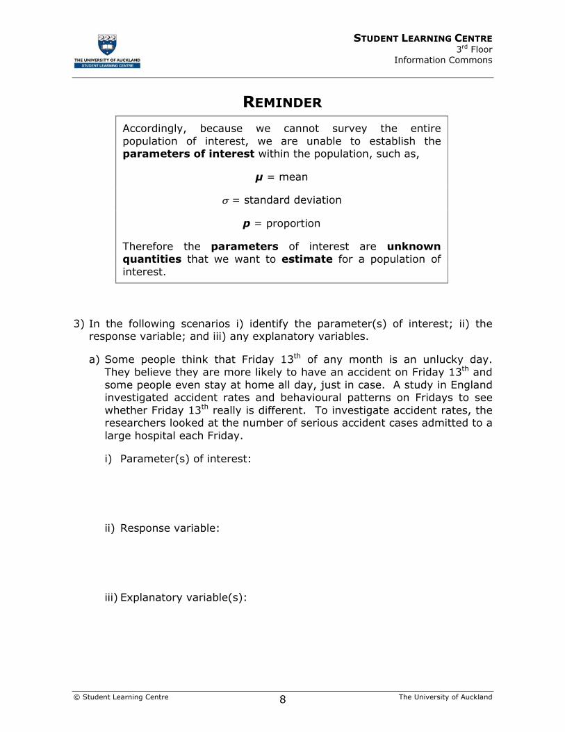
REMINDER

Accordingly, because we cannot survey the entire population of interest, we are unable to establish the parameters of interest within the population, such as,

µ = mean

σ = standard deviation

p = proportion

Therefore the parameters of interest are unknown quantities that we want to estimate for a population of interest.

3) In the following scenarios i) identify the parameter(s) of interest; ii) the response variable; and iii) any explanatory variables.

a) Some people think that Friday 13th of any month is an unlucky day. They believe they are more likely to have an accident on Friday 13th and some people even stay at home all day, just in case. A study in England investigated accident rates and behavioural patterns on Fridays to see whether Friday 13th really is different. To investigate accident rates, the researchers looked at the number of serious accident cases admitted to a large hospital each Friday.

i) Parameter(s) of interest:

ii) Response variable:

iii) Explanatory variable(s):



b) A researcher wished to investigate whether there was a relationship between the weight of 10-year old boys and whether they played rugby or soccer.




c) The manager of a shop that hires videos and DVDs is interested in how many DVDs a customer hires per week in order to decide whether to reward regular customers by giving them their next DVD hire free of charge.






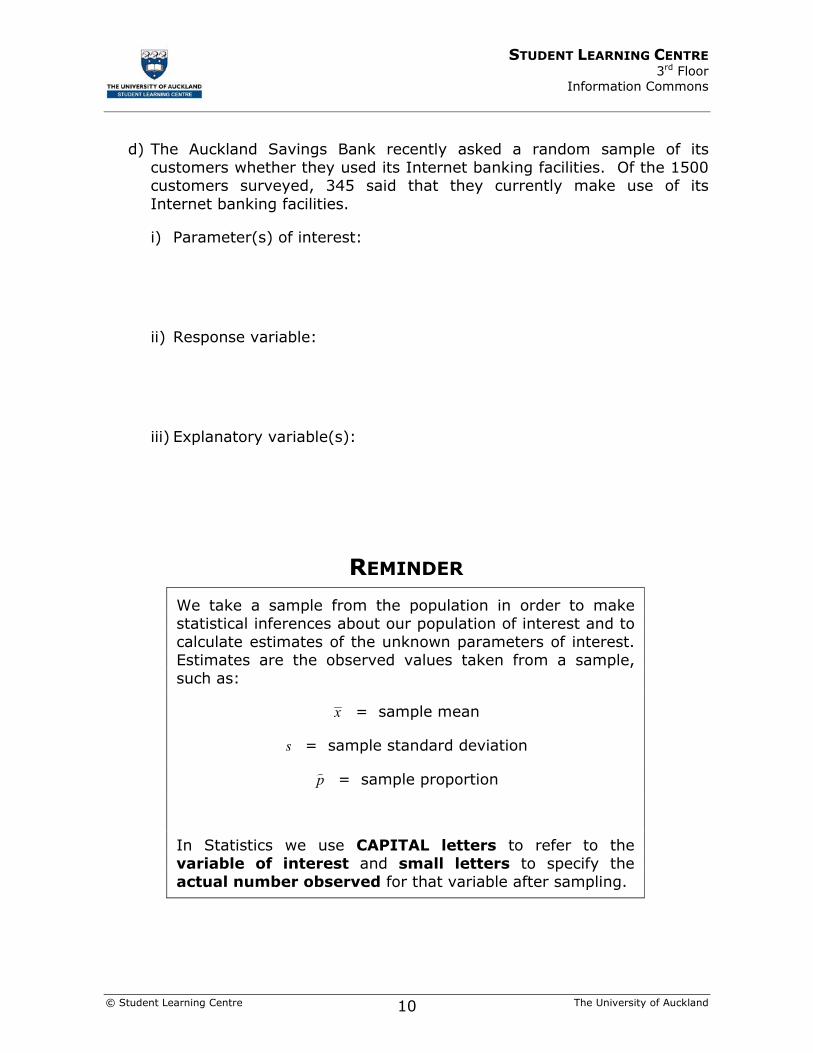
d) The Auckland Savings Bank recently asked a random sample of its customers whether they used its Internet banking facilities. Of the 1500 customers surveyed, 345 said that they currently make use of its Internet banking facilities.




REMINDER

We take a sample from the population in order to make statistical inferences about our population of interest and to calculate estimates of the unknown parameters of interest. Estimates are the observed values taken from a sample, such as:

x = sample mean

s = sample standard deviation

p) = sample proportion

In Statistics we use CAPITAL letters to refer to the variable of interest and small letters to specify the actual number observed for that variable after sampling.



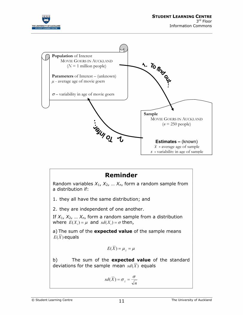
Reminder Random variables X1, X2, … Xn, form a random sample from a distribution if:

1. they all have the same distribution; and

2. they are independent of one another.

If X1, X2, … Xn, form a random sample from a distribution where µ=)( iXE and σ=)( iXsd then,

a) The sum of the expected value of the sample means )(XE equals

µµ ==X

XE )(

b) The sum of the expected value of the standard deviations for the sample mean )(Xsd equals

nXsd

X

σσ ==)(

Population of Interest MOVIE GOERS IN AUCKLAND

(N = 1 million people)

Parameters of Interest – (unknown) µ - average age of movie goers

σ – variability in age of movie goers

Sample MOVIE GOERS IN AUCKLAND

(n = 250 people)

Estimates – (known) x - average age of sample

s - variability in age of sample



4) A large NZ book warehouse sends books out to its subsidiary warehouses throughout the country. The books are sent out in batches of 50. It found from a sample of data collected that the average width of its different book titles in a batch is 900mm. Which one of the following statements is false?

a) The sample mean x = 900mm is an estimate of µ.

b) The sample mean x = 900mm is an observation from an approximate Normal distribution with unknown µ.

c) µ is the average width of its different book titles in a batch.

d) If a second sample were taken, the population mean µ would not change.

e) The variability of the sample mean, X , increases as we increase the size of the sample on which it is based.

5) The NZ Herald, 14 August 2001, reported the results of a two-year study at Hong Kong’s Kwong Wah Hospital. The study comprised 5450 impotent men who were given Viagra at the hospital. Assume this is a random sample of all impotent Chinese men and that for 926 of the men Viagra did not work. However, suppose that it is also known that Viagra works for 78% of impotent Western males.

Which one of the following statements is true?

a) The proportion of Chinese men in the sample for whom Viagra works is both an estimate value and a parameter value.

b) The proportion of Chinese men in the sample for whom Viagra works is an estimate value whereas the 78% of impotent Western males for whom Viagra works is a parameter value.

c) The proportion of Chinese men in the sample for whom Viagra works and the 78% of impotent Western males for whom Viagra works are both parameters values.

d) The proportion of Chinese men in the sample for whom Viagra works and the 78% of impotent Western males for whom Viagra works are neither estimates nor parameter values.

e) The proportion of Chinese men in the sample for whom Viagra works is a parameter value whereas the 78% of impotent Western males for whom Viagra works is an estimate value.



Reminder A population with a Normal distribution has a symmetric bell-shape centred on the mean of the population.

For a continuous random variable from a population with a Normal distribution the probability that it lies within:

1 σ of the µ is 68%

2 σ of the µ is 95%

3 σ of the µ is 99.7%

6) Do we know the shape of the population we are sampling from? Briefly explain.

7) If we are sampling from a Normal distribution, what is the shape X ?

8) If we are sampling from a non-Normal distribution:

a) What theorem helps us find out about the sample of the distribution of X ?

b) What aspect of the sample affects how well the theorem works?



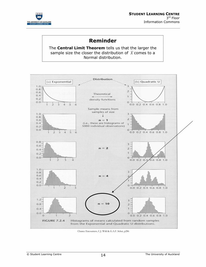
Chance Encounters, C.J. Wild & G.A.F. Seber, p286

Reminder The Central Limit Theorem tells us that the larger the sample size the closer the distribution of X comes to a

Normal distribution.



If X is from a “well-behaved” distribution (i.e. symmetric, no outliers) the Central Limit Theorem works reasonably fast.

For example, n = 10 may be sufficient

In general, n = 30 works well for most distributions except distributions that are severely skewed or have large outliers.

If the distribution is severely skewed, n = 50 should be sufficient.

Reminder

Even if the distribution of X is non-Normal, the distribution of X will be Normal for a sufficiently large sample size n.

Reminder X is an unbiased estimator of µ because µ=)(XE .

The n

Xsd σ=)( it is not a useful measure of the precision of x ,

because we do not know the value of σ. Therefore, we have to use the standard error of the sample mean to estimate the precision of x as an estimate of µ.

The standard error of x = sizesampledeviationstandardsample

= nsxse =)(

Reminder

When we have to estimate σ for the )(Xsd we get the )(xse and have to use the Student’s t-distribution



9) The Student’s t-distribution describes another family of distributions with a

parameter called the . The formula for df = . When

df = ∞ the distribution curve becomes indistinguishable from the

distribution.

10) Suppose that X1, X2, … Xn is a random sample of size n from a

distribution with mean µ and standard deviation σ. Let X represent the

sample mean. Fill in the gaps:

a) Since = µ, x is an estimate of µ.

b) If X is Normally distributed then

ns

X µ−is a random variable with a

distribution with parameter , where df =

.



c) If X is Normally distributed then

n

Xσ

µ−is a random variable with a

distribution with parameters

d) The Central Limit Theorem says that for large samples from a non-

Normal distribution, the distribution of )(Xsd

X µ−is the standard

Normal distribution.

e) The Student's t-distribution with parameter degrees of freedom, df,

shows variability as df .


Information Commons


SECTION TWO CONFIDENCE INTERVALS & SIGNIFICANCE TESTING



1) In hypothesis testing and confidence intervals we use

information to make inferences about

2) A significance test determines the (circle one) strength / size of the

evidence the value, while a confidence

interval determines the (circle one) strength / size of the effect.

3) A contains the true value of a

parameter for 95% of taken.

Reminder

Confidence interval: estimate ± t standard errors

)ˆ()2/(ˆ θαθ setdf±

t-test statistic: t0 =estimate - hypothesised value

standard errors

t0 =ˆ θ −θ0

se( ˆ θ )

θ = µ: ˆ θ = x , se(x ) =sX

n, df = n −1

θ = µ1 – µ2 :

For means, the size of the t-multiplier depends both on the desired level of confidence and the degrees of freedom (df).

)1,1(Min

,)(se)(se)(se

ˆ

21

2

2

1

22

22

121

21

21

−−=

+=+=−

−=

nndfns

ns

xxxx

xxθ



4) An insurance company wanted to know whether the average repair costs for cars that had been involved in ‘fender benders’ was still roughly $1,000. The company had calculated this estimate 5 years earlier. The repair cost estimates (in dollars) for a sample of 16 ‘fender bender’ incidents was obtained:

700, 1500, 2000, 850, 1450, 2300, 1800, 2000, 800, 1300, 2000, 800, 1100, 2500, 1650, 1950

25001500500

Repair cost estimates

Boxplot of Repair cost estimates(with Ho and 95% t-confidence interval for the mean)

[ ]X_

Ho

P-Value (approx): > 0.1000R: 0.9813W-test for Normality

N: 16StDev: 572.676Average: 1543.75

2500200015001000

.999

.99

.95

.80

.50

.20

.05

.01

.001

Pro

babi

lity

Repair cost

Normal Probability Plot

Descriptive Statistics: Repair cost estimates Variable N Mean Median TrMean StDev SE Mean Repair c 16 1544 1575 1536 573 143 Variable Minimum Maximum Q1 Q3 Repair c 700 2500 913 2000



One-Sample T: Repair cost estimates Test of mu = 1000 vs mu not = 1000 Variable N Mean StDev SE Mean Repair cost 16 1544 573 143 Variable 95.0% CI T P Repair cost ( ****, ****) **** 0.002

a) State the parameter of interest θ (as a symbol or symbols and words)

b) Identify the hypotheses:

i) H0:

ii) H1:

c) Identify the estimate θ̂ (using a symbol and a number):

d) Calculate se(θ̂ ):

e) State the value of df:

f) Calculate the t-test statistic:



g) Calculate the 95% confidence interval:

h) Interpret the confidence interval:

i) Does the confidence interval contain the parameter of interest θ? Briefly discuss:



5) Identify which one of the following statements about confidence intervals are true or false?

a) If a large number of researchers independently perform studies to estimate µ, about 95% of them will catch the true value of µ in their 95% confidence intervals.

b) Large samples tend to yield narrower 95% confidence intervals than small samples.

c) A two-standard error interval will always capture the true value of µ.

d) In the long run, if we repeatedly take samples and calculate a 95% confidence interval from each sample, we expect that 95% of the intervals will contain the true value of µ.

e) A point estimate is preferred to a confidence interval because the interval summarises the uncertainty due to sampling variation.

f) The margin of error is the quantity added to and subtracted from, the estimate to construct the interval.

g) The standard error used to construct the interval will be identical for all samples of the same size.

h) If I plan to do a study in the future in which I will take a random sample and calculate a 90% confidence interval, there is a 90% chance that I will catch the true value of µ in my interval.

i) The size of the multiplier t depends on only the sample size and not the desired confidence level.

j) The process of using sample data to construct an interval estimate for a population mean is an example of statistical inference.



6) When conducting a statistical test, the value is

tested as a possible value for the parameter.

7) testing is a method used to deal with the uncertainty

about the value of a parameter caused by the

in estimates.

Reminder H0 denotes the null hypothesis versus H1, which denotes the alternative hypothesis.

The null hypothesis is not equal to the parameter of interest. It is a best guess as to what we think the parameter is interest is - remember that the parameter of interest is an unknown quantity.

H1 specifies the type of departure from H0 that we expect to detect and corresponds to the research hypothesis.

The 3 alternative hypotheses that are possible when testing H0 are:

H1: θ ≠ θ0

H1: θ > θ0

H1: θ < θ0

The measure of evidence against the null hypothesis is called a P-value.

Under the assumption that the null hypothesis is true (but REMEMBER IT IS NOT), then the p-value is the probability that sampling variation would produce an estimate that is further away from the hypothesised value than the estimate we obtained from our data.

Interpreting the size of a P-value

>0.12 = no evidence against H0

0.10 = weak evidence against H0

0.05 = some evidence against H0

0.01 = strong evidence against H0

<0.001 = very strong evidence against H0



8) H0 is true, if we have no evidence against H0. True / False

9) If a P-value is large, then H0 is plausible. True / False

10) If we test at the 5% level how many true null hypotheses will we reject

in the long run?

11) The smaller the P-value, the the evidence

H0.

12) A two-sided test of H0: θ = θ0 is significant at the 5% level, if θ0 lies

(circle one) inside / outside a confidence interval for θ.

Reminder

To calculate the test-statistic:

)ˆ(

ˆ

errorstandardvalueedhypothesizestimate 0

0 θθθ

set

−=

−=

To calculate the p-value for the 3 alternative hypotheses:

H1: θ ≠ θ0 )(2 0tTprP ≥=

H1: θ > θ0 )( 0tTprP ≥=

H1: θ < θ0 )( 0tTprP ≤=

To calculate a confidence interval

)ˆ(ˆ)( θθ setestimatesetestimate ×±=×±



Two Independent samples

Asia Europe

0

50000

100000

150000

Boxplots of Asia and Europe(means are indicated by solid circles)

Average: 40977.7StDev: 24074.3N: 20

W-test for NormalityR: 0.9830P-Value (approx): > 0.1000

0 20000 40000 60000 80000

.001

.01

.05

.20

.50

.80

.95

.99

.999

Pro

babi

lity

Asia





N: 28StDev: 48643.5Average: 81239.8

150000100000500000

.999

.99

.95

.80

.50

.20

.05

.01

.001

Pro

babi

lity

Europe


Two-Sample T-Test and CI: Asia, Europe Two-sample T for Asia vs Europe N Mean StDev SE Mean Asia 20 40978 24074 5383 Europe 28 81240 48644 9193 Difference = mu Asia - mu Europe Estimate for difference: -40262 95% CI for difference: (-61776, -18748) T-Test of difference = 0 (vs not =): T-Value = -3.78 P-Value = 0.001 DF = 41

13) Two Sample t-Test and Confidence Interval

a) State the parameter of interest θ (in a symbol or symbols and words)



b) Identify the hypotheses

i) H0:

ii) H1:

c) Identify the estimate θ̂ (using a symbol or symbols and a number)

d) Calculate se(θ̂ )



e) Comment on the plots and the assumptions associated with this test.

f) Find the P-value and interpret.

g) Identify which of the following statements are true or false. Briefly correct the false statements.

i) With 95% confidence, we estimate that the price for cars in the Asia region is somewhere between $18,748 and $61,776 less than the price for cars in the European region.

ii) With 95% confidence, we estimate that the average price for cars in the Asia region is somewhere between $18,748 and $61,776 more than the average price for cars in the European region.



iii) The underlying mean price for cars in the Asia region is between $18,748 and $61,776 less than the underlying mean price for cars in the European region. We can make this statement with confidence 19 out of 20 times.

iv) The underlying mean price for cars in the Asia region is between $18,748 and $61,776 more than the underlying mean price for cars in the European region. We can make this statement with confidence 1 out of 20 times.

v) The underlying mean price for cars in the European region is between $18,748 and $61,776 more than the underlying mean price for cars in Asia the region. We make this statement with 95% confidence.

Reminder We have to distinguish between independent samples and related samples.

E.g., a random sample of 15 people are asked to rate their opinion of a product prior to using the product, on a scale of 1 to 5 (1=poor quality; 5=excellent quality). The same sample of 15 people is then asked to rate their opinion of the product after a free 1-month trial using the same scale. The measurement of opinion is being taken twice on each person in the sample (before use and after use) and therefore this data is related.

With related or paired data we analyse the differences using a 1-sample t-test.



Paired data

14) The marketing manager of a new weight loss program wanted to verify the claim that people who used the product could loss on average 10 kilos after taking the product for more than 4 weeks. A random sample of 20 volunteers was selected and their weight measurements recorded before using the product and then again after 5 weeks of using the product. The data results are listed below:

Paired T for Before - After N Mean StDev SE Mean Before 20 67.16 12.93 2.89 After 20 64.45 10.80 2.41 Difference 20 2.710 3.855 0.862 95% CI for mean difference: (0.906, 4.514) T-Test of mean difference = 0 (vs not = 0): T-Value = 3.14 P-Value = 0.005

a) Identify the parameter of interest

1050Differences in Weight (kg)

Boxplot of Differences(with Ho and 95% t-confidence interval for the mean)

[ ]X_

Ho


N: 20StDev: 3.85463Average: 2.70991

1050

.999

.99

.95

.80

.50

.20

.05

.01

.001

Pro

babi

lity

Difference




b) Identify the hypotheses

i) H0:

ii) H1:

c) Interpret the p-value in terms of the study.

d) Interpret the confidence interval in terms of the study.



More than two groups

Reminder One-way analysis of variance (ANOVA) uses an F-test to compare the means of 3 or more populations, in relation to one factor of interest, using independent samples.

H0 = all of the underlying true means are identical

vs

H1 = differences exist between some of the true means

2

2

0W

B

ssf = where df1 = k-1, df2 = ntot – k

Assumptions are that:

1. data Normally distributed (test robust against departures from Normality)

2. standard deviations of samples are equal ~

2sdsmallest

sdlargestratio <=

3. samples are independent

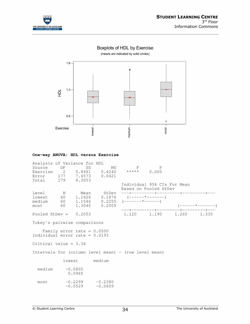
15) HDL cholesterol is known as the “good cholesterol” as it is associated with lower risks of problems like heart disease. The following data were collected on men working in New Zealand companies. The men were divided into exercise groups by the amount of exercise they reported. Levels of exercise were classified as lowest, medium, and most. Sixty men were randomly sampled from each exercise group, and their HDL cholesterol level was measured.



low

est

med

ium

mos

t

0.8

1.3

1.8

Exercise

HD

L

Boxplots of HDL by Exercise(means are indicated by solid circles)

One-way ANOVA: HDL versus Exercise Analysis of Variance for HDL Source DF SS MS F P Exercise 2 0.8481 0.4240 ***** 0.000 Error 177 7.4573 0.0421 Total 179 8.3053 Individual 95% CIs For Mean Based on Pooled StDev Level N Mean StDev ---+---------+---------+---------+--- lowest 60 1.1626 0.1876 (------*-------) medium 60 1.1546 0.2255 (-------*------) most 60 1.3040 0.2009 (------*-------) ---+---------+---------+---------+--- Pooled StDev = 0.2053 1.120 1.190 1.260 1.330 Tukey's pairwise comparisons Family error rate = 0.0500 Individual error rate = 0.0193 Critical value = 3.34 Intervals for (column level mean) - (row level mean) lowest medium medium -0.0805 0.0965 most -0.2299 -0.2380 -0.0529 -0.0609



a) Identify the parameter of interest:

b) Identify the hypotheses:

i) H0:

ii) H1:

c) Check that the assumptions for this test are correct.

d) Calculate the value of the F-statistic



e) Interpret the P-value in terms of the study.

f) Interpret the confidence intervals for those pairs that are significant at the 5% level.


Information Commons


SECTION THREE CHI-SQUARE TESTING & REGRESSION



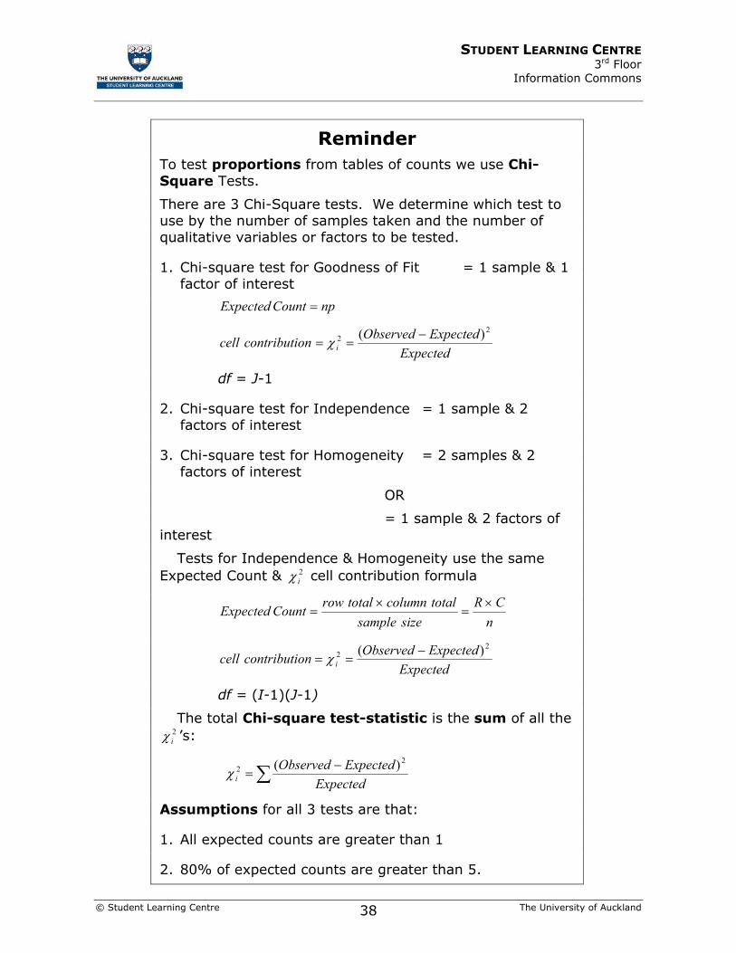
Reminder To test proportions from tables of counts we use Chi-Square Tests.

There are 3 Chi-Square tests. We determine which test to use by the number of samples taken and the number of qualitative variables or factors to be tested.

1. Chi-square test for Goodness of Fit = 1 sample & 1 factor of interest

npCountExpected =

Expected

ExpectedObservedoncontributicell i

22 )( −

== χ

df = J-1

2. Chi-square test for Independence = 1 sample & 2 factors of interest

3. Chi-square test for Homogeneity = 2 samples & 2 factors of interest

OR

= 1 sample & 2 factors of interest

Tests for Independence & Homogeneity use the same Expected Count & 2

iχ cell contribution formula

n

CRsizesample

totalcolumntotalrowCountExpected ×=

×=

Expected

ExpectedObservedoncontributicell i

22 )( −

== χ

df = (I-1)(J-1)

The total Chi-square test-statistic is the sum of all the 2iχ ’s:

∑ −=

ExpectedExpectedObserved

i

22 )(χ

Assumptions for all 3 tests are that:

1. All expected counts are greater than 1

2. 80% of expected counts are greater than 5.



The paper “Family Planning: Football Style. The Relative Age Effect in Football.” investigated the relationship between month of birth and achievement in sports for men. Birth dates were collected on all players in teams competing in the 1990 World Cup soccer games, and they are summarised below.

Birthdays by Quarter Frequency

Q1: Aug-Oct 150

Q2: Nov-Jan 138

Q3: Feb-Apr 140

Q4: May-Jul 100

Total 528

The paper claims that the distribution of players’ birth dates is not random and that the number of players is related to the ‘Quarters of the football year’. The claim is based on the results of a Chi-square test for goodness of fit.

1) The hypotheses for such a test are:

(a) H0: Over a year, the greatest proportion of players are born in Q1: Aug-Oct.

H1: Over a year, the greatest proportion of players are not born in Q1: Aug-Oct.

(b) H0: 25% of all players are born in each quarter.

H1: There are at least two quarters in which the proportion of all players born is not 25%.

(c) H0: The proportion of players born in each quarter is different for each quarter.

H1: The proportion of players born in each quarter is same for each quarter.

(d) H0: The proportion of players born in each quarter is 0.28, 0.26, 0.27 and 0.19

H1: The proportion of players born in each quarter is not those given in H0.

(e) H0: 25% of all players are born in each quarter.

H1: There are no quarters in which the proportion of all players born is 25%.



2) Complete the following table of Expected Counts and Cell Contributions for the Birthdays by Quarter data.

Birthdays by Quarter Frequency Expected 2iχ

Q1: Aug-Oct 150

Q2: Nov-Jan 138

Q3: Feb-Apr 140

Q4: May-Jul 100

Total 528

3) Using the Minitab output below to calculate the P-value for the Chi-square test in question 2) and interpret the results.

Cumulative Distribution Function Chi-Square with 3 DF x P( X <= x ) 10.9697 0.9881

4) Have the assumptions for this test been met?



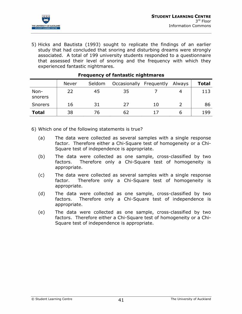
5) Hicks and Bautista (1993) sought to replicate the findings of an earlier study that had concluded that snoring and disturbing dreams were strongly associated. A total of 199 university students responded to a questionnaire that assessed their level of snoring and the frequency with which they experienced fantastic nightmares.

Frequency of fantastic nightmares

Never Seldom Occasionally Frequently Always Total

Non-snorers

22 45 35 7 4 113

Snorers 16 31 27 10 2 86

Total 38 76 62 17 6 199

6) Which one of the following statements is true?

(a) The data were collected as several samples with a single response factor. Therefore either a Chi-Square test of homogeneity or a Chi-Square test of independence is appropriate.

(b) The data were collected as one sample, cross-classified by two factors. Therefore only a Chi-Square test of homogeneity is appropriate.

(c) The data were collected as several samples with a single response factor. Therefore only a Chi-Square test of homogeneity is appropriate.

(d) The data were collected as one sample, cross-classified by two factors. Therefore only a Chi-Square test of independence is appropriate.

(e) The data were collected as one sample, cross-classified by two factors. Therefore either a Chi-Square test of homogeneity or a Chi-Square test of independence is appropriate.



Results for: Snoring and Nightmares Chi-Square Test: Never, Seldom, Occasionally, Frequently, Always Expected counts are printed below observed counts Never Seldom Occasion Frequent Always Total 1 22 45 35 7 4 113 21.58 ***** 35.21 9.65 3.41 2 16 31 27 10 2 86 16.42 32.84 26.79 **** 2.59 Total 38 76 62 17 6 199 Chi-Sq = 0.008 + 0.079 + 0.001 + ***** + 0.103 + 0.011 + 0.104 + 0.002 + 0.958 + 0.136 = 2.131 DF = ***, P-Value = 0.712

7) There are four missing values in the Chi-square test table. Calculate the missing values.

(a)Expected count for a Non-snorer who Seldom has nightmares.

(b) Expected count for a Snorer who Frequently has nightmares.

(c) Cell contribution for a Non-snorer who Frequently has nightmares.



(d) Degrees of freedom for the test.

8) A Warning Message is also generated by Minitab. Do we have any reason to doubt the validity of the test?

9) Interpret the P-value in terms of the study.



Reminder Regression looks at the relationship between two quantitative variables. Y is the response variable and X is the explanatory variable.

X is used to explain or predict the behaviour of Y.

We use a least squares regression line where xy 10

ˆˆˆ ββ += with the following assumptions:

1. Linear relationship between X and Y

2. Random errors are Normally distributed (with µ=0)

3. Random errors all have the same σ regardless of x.

4. Random errors are all independent.

The correlation coefficient r is used as a measure of linear association between X and Y.

Correlation tests that there is an association between X and Y by treating both variables equally. Correlation DOES NOT imply causation.

1. r = 1, then X and Y have a perfect positive linear relationship

2. r = -1, then X and Y have a perfect negative linear relationship

3. r = 0, then X and Y have no linear relationship

1) Fill in the gaps.

(a) In a straight-line graph, changes by a amount with

each unit change in

(b) The regression model consists of linear trend plus

(c) 10β̂ and 10β̂ are of the parameters β0 and β1



(d) The least squares estimates minimise the sum of the

squared.

(e) The prediction interval for a particular value will always be

than the confidence interval for the mean.

(f) It is unsafe to predict values the range of the

observed data.

(g) A correlation coefficient which is close to zero indicates either a

relationship or relationship between X and Y.

Reminder H0: β1 = 0 testing for no linear relationship

df = n – 2

residual = ii yy ˆ− = observed - expected



2) How crucial is the start in the 100m sprint at Olympic level? Twenty men’s 100m races were run at the 1996 Olympic Games at Atlanta resulting in 168 finishes by athletes. A sample of 30 finishes was taken and the following analysis performed to determine whether the running time was associated with the athlete’s reaction time off the starting block.

Regression Analysis: Running versus React The regression equation is Running = 9.32 + 5.87 React Predictor Coef SE Coef T P Constant 9.3241 0.5789 16.11 0.000 React 5.870 3.382 1.74 0.094 S = 0.4297 R-Sq = 9.7% R-Sq(adj) = 6.5% Analysis of Variance Source DF SS MS F P Regression 1 0.5561 0.5561 3.01 0.094 Residual Error 28 5.1695 0.1846 Total 29 5.7257

0.12 0.17 0.22

9.5

10.5

11.5

React

Run

ning

Scatter plot of Reaction Time vs Running Time

10.610.510.410.310.210.110.0

1.0

0.5

0.0

-0.5

Fitted Value

Res

idua

l

Residuals Versus the Fitted Values(response is Running)

Average: -0.0000230StDev: 0.422209N: 30

W-test for NormalityR: 0.9425P-Value (approx): < 0.0100

-0.5 0.0 0.5 1.0

.001

.01

.05

.20

.50

.80

.95

.99

.999

Pro

babi

lity

Residuals

Normal Probability Plot of Residuals



h) Identify the hypotheses

i) H0:

ii) H1:

i) Write out the least squares equation for this model.

j) An athlete whose reaction time was 0.123 seconds would be expected to

have a running time of seconds?

k) An athlete with a reaction time of 0.167 seconds had a running time of 10.83 seconds. Calculate the prediction error or residual for this athlete.



l) Comment on the associated plots with reference to the assumptions.

m) Based on the results of the regression analysis above, which one of the following statements is the best overall conclusion?

i) The faster an athlete reacts the faster he will run.

ii) The slower an athlete reacts the slower he will run.

iii) xy 3241.9870.5ˆ +=

iv) There is evidence that an athlete’s running time is related to his reaction time.

v) There is weak evidence that an athlete’s running time is related to his reaction time.

n) Using a t-multiplier of 2.048 build a confidence interval for the analysis and interpret.



3) Identify whether the following statements are true or false.

(a) Regression analysis requires 1 continuous random variable and 1 qualitative variable.

(b) In a straight line graph, Y changes by a fixed amount with each unit changed in X.

(c) When a least-squares regression line is fitted to the data, the sum of the prediction errors is zero.

(d) For a particular x-value, the standard error used to calculate the prediction interval for Y allows for uncertainty about the true values of the intercept and the slope of the line, as well as the uncertainty due to random scatter.

(e) The errors from a regression analysis are assumed to be normally distributed with a mean of zero.

(f) If X and Y are correlated we can say that X causes Y.

(g) The correlation between two variables, X and Y is 0.7. As the value of X increases, the value of Y tends to decrease.

(h) The correlation between two variables, X and Y is 0.7. As the value of X increases, the value of Y tends to increase.

(i) A correlation coefficient, r, of zero indicates that there is no relationship between two variables.

(j) A linear regression model should never be used without examining the appropriate boxplot.

(k) A single outlier can exert a strong influence over the least squares line.


Information Commons


STATS 10X FORMULA SHEET



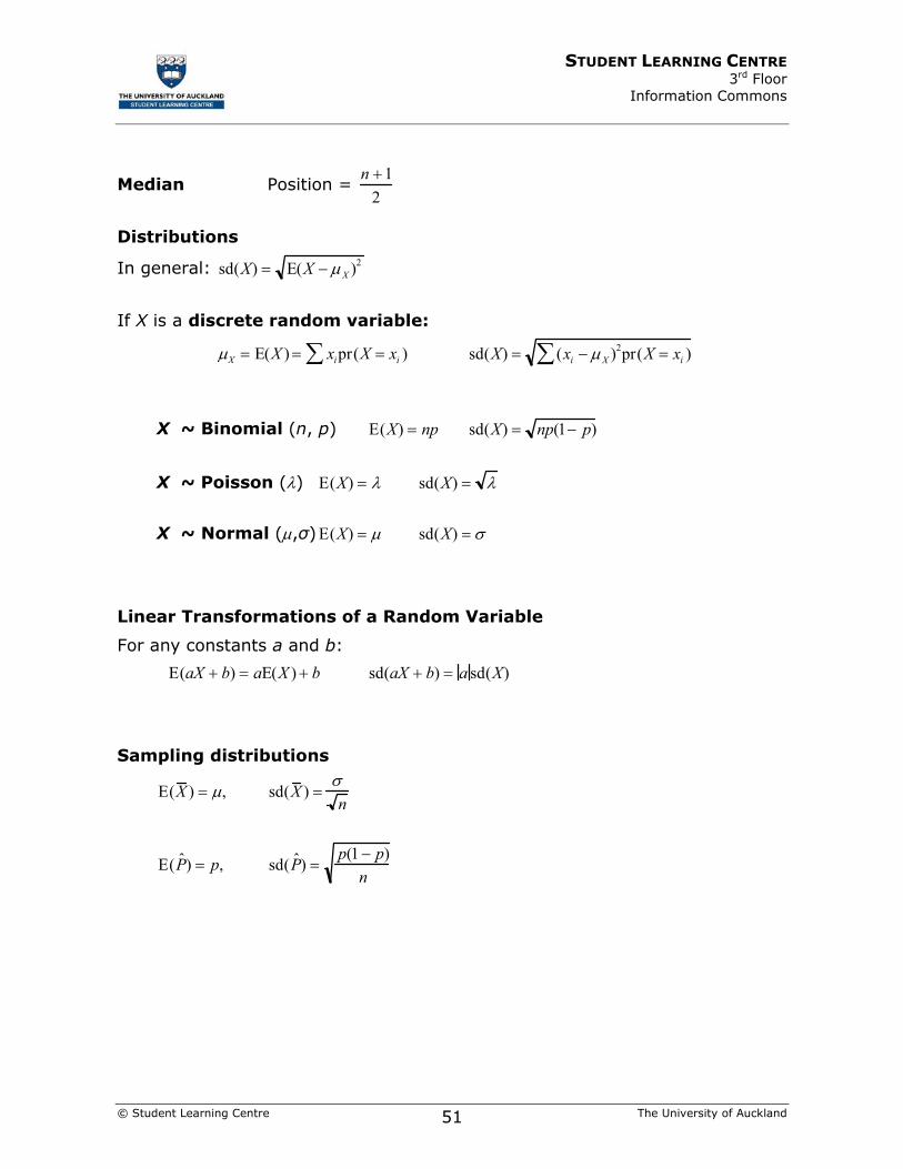
Median Position = n +1

2

Distributions

In general: sd(X) = E(X − µX )2

If X is a discrete random variable:

µX = E(X ) = xipr(X = xi )∑ sd(X) = (xi − µX )2∑ pr(X = xi )

X ~ Binomial (n, p) E(X) = np sd(X) = np(1− p)

X ~ Poisson (λ) E(X) = λ sd(X) = λ

X ~ Normal (µ,σ) E(X) = µ sd(X) = σ

Linear Transformations of a Random Variable

For any constants a and b:

E(aX + b) = aE(X ) + b sd(aX + b) = a sd(X) Sampling distributions

E(X ) = µ, sd(X ) =σn

E( ˆ P ) = p, sd( ˆ P ) =p(1 − p)

n



Standard error of a difference (independent estimates)

se( ˆ θ 1 − ˆ θ 2 ) = se( ˆ θ 1 )2 + se( ˆ θ 2 )2 Confidence intervals & t-tests

Confidence interval: estimate ± t standard errors

ˆ θ ± tdf (α / 2)se( ˆ θ )

t-test statistic: t0 =estimate - hypothesised value

standard errors

t0 =ˆ θ −θ0

se( ˆ θ )

Applications

Mean µX : ˆ θ = x , se(x ) =sX

n, df = n −1

Proportion p : ˆ θ = ˆ p , se( ˆ p ) =ˆ p (1− ˆ p )

n, df = ∞

Difference between two means µ1 - µ2: ˆ θ = x 1 − x 2 (independent samples),

se(x 1 − x 2 ) = se(x 1)2 + se(x 2 )2 =

s1

2

n1

+s

2

2

n2

, df = Min(n1 −1,n2 −1)

Difference in proportions p1 - p2: ˆ θ = ˆ p 1 - ˆ p 2 with

(a) Proportions from two independent samples of sizes n1, n2 respectively

se( ˆ p 1 − ˆ p 2 ) =ˆ p 1 (1− ˆ p 1)

n1

+ˆ p 2(1 − ˆ p 2 )

n2

, df = ∞

(b) One sample of size n, several response categories

se( ˆ p 1 − ˆ p 2 ) =ˆ p 1 + ˆ p 2 − ( ˆ p 1 − ˆ p 2 )2

n, df = ∞



(c) One sample of size n, many yes/no items

se( ˆ p 1 − ˆ p 2 ) =Min( ˆ p 1 + ˆ p 2 , ˆ q 1 + ˆ q 2 ) − ( ˆ p 1 − ˆ p 2 )2

n, df = ∞

where ˆ q 1 = 1− ˆ p 1 and ˆ q 2 =1 − ˆ p 2

The F-test (ANOVA)

f0 =sB

2

sW2 df1 = k − 1 df2 = ntot - k

The Chi-square test

χ02 =

(observed − expected)2

expectedall cells in the table∑

For one-way tables: df = J-1

For two-way tables:

Expected count in cell (i, j) =RiCj

n

df = (I −1)(J −1)

Regression

Fitted least-squares regression line: xy 10ˆ+ˆ=ˆ ββ

Inference about the intercept, β0, and the slope, β1 : df = n - 2

stats 20x workshops - aucklandleila/booklet.pdf · 9 test and examination skills ... 9 tutorial...

Documents