stefanie stantcheva fall 2016 - harvard university

Lecture 12: Social Security, Retirement and DisabilityStefanie Stantcheva

Fall 2016

1 69

GOALS OF THIS LECTURE

(1) Understand main theories behind social security.(2) Empirical effects of social security.

2 69

RETIREMENT PROBLEM

Life-Cycle: Individuals ability to work declines with aging but individualscontinue to live after they are unwilling/unable to workStandard Life-Cycle Model Prediction: Absent any government program,rational individual would save while working to consume savings whileretired [draw Modigliani graph]Optimal saving problem is extremely complex: uncertainty in returns tosaving, in life-span, in future ability/opportunities to work, in futuretastes/healthIn practice: When govt was small ⇒ Many people worked till unable to(often till death) and then were taken care of by family members (paygosystem not funded) [US elderly poverty rate very high before SocialSecurity]

3 69

GOVT INTERVENTION IN RETIREMENT POLICY

Actual Retirement Programs: All OECD countries implement substantialretirement programs (substantial share of GDP around 6-10%, US smalleraround 4%)Started in first part of 20th century and have been growing. Commonstructure:Individual pay social security contributions (payroll taxes) while workingand receive retirement benefits when they stop working till the end of theirlife (annuity)Various types of retirement programs (private or public):

(a) Funded vs. Unfunded, (b) Defined Benefits vs. Defined Contributions, (c)Mandatory vs. Voluntary, (d) Universal vs. Means-tested, (e) Annuitizedbenefits vs. lumpsum4 69

FUNDED VS. UNFUNDED PROGRAMS

Unfunded (pay-as-you-go): benefits of current retirees are paid out ofcontributions from current workers [generational link]current benefits = current contributionsFunded: workers contributions are invested in financial assets and willpay for benefits when they retire [no generational link]current benefits = past contributions + market returns on pastcontributions

5 69

Defined Contributions vs. Defined Benefits

Defined Contributions (DC): System specifies the level of contributions[e.g., 10% of earnings]. Benefits then depend on level of contributions andreturns on contributions.Defined Benefits (DB): System specifies the level of benefits [e.g., 60% ofaverage earnings during career]. Contributions adjusted to meet requiredlevel of benefits.DC pro: Easier to implement and contributions are not perceived as a “tax”DC con: Benefits are risky. Risk in benefits worse than risk in contributions[as workers can adjust and absorb shocks more easily than retirees]

6 69

EXAMPLES

1) Unfunded DB: most public retirement programs (such as Social Securityin the US)2) Funded DB: traditional US private employer pension plans [e.g., annualbenefits = 2.5%*years worked*last salary], a govt DB retirement programcould also be funded [govt invests payroll taxes]3) Funded DC: new US private employer pensions plans [401(k)s]: workercontributes fraction of salary and invests contributions in financial assets.4) Unfunded DC: Notional accounts in some government retirementprograms (Sweden): payroll taxes yield fictitious returns and benefits arebased on contributions plus this fictitious (notional) return.

7 69

WHY SHOULD GOVERNMENT INTERVENE?

1) Individual Failures: (MOST IMPORTANT) Individuals would not saveadequately for retirement on their own (information and self-controlproblems).Paternalism: govt imposes its preferences against individuals ⇒ Individualsshould oppose govt programBehavioral: individuals understand that they have problems and welcomegovt intervention2) Market Failures: Adverse selection in annuitization market3) Redistribution:(a) Within Generations: Retirement programs can redistribute based onlife-time earnings (instead of annual)(b) Across Generations: Retirement programs can redistribute acrosscohorts (so does govt debt) 8 69

SOURCES OF RETIREMENT INCOME

1) Govt provided retirement benefits (US Social Security): US: For 2/3 ofretirees, SS is more than 50% of income. 1/3 of elderly households dependalmost entirely on SS.2) Home Ownership: 75% of US elderly are homeowners3) Employer pensions (tax favored): 40-45% of elderly US households haveemployer pensions. Two types:a) Traditional: DB and mandatory: employer carries full risk [in sharpdecline, many in default]b) New: DC and elective: 401(k)s, employee carries full risk60% of workers have access to empl. pensions, 45% contribute4) Supplementary individual elective pensions (tax favored): IRAs andKeoghs (Keoghs for the self-employed)5) Extra savings through non-tax favored instruments: significant only forwealthy minority [=10% of retirees]

9 69

MODEL: MYOPIC SAVERS

1) Some individuals are rational:max u(c1) + δu(c2) subject to

c1 + s = w and c2 = s · (1+ r), c1 + c2/(1+ r) = w

FOC: u′(c2)/u′(c1) = 1/[(1+ r)δ ], let s∗ be optimal savingExample: If δ = 1 and r = 0 then s∗ = w/2 and c1 = c2 = w/2

2) Some individuals are myopic:max u(c1) subject to

c1 + s = w and c2 = s · (1+ r) ⇒ c1 = w and s = c2 = 0

10 69

MODEL: MYOPIC SAVERS

Social welfare is always u(c1) + δu(c2)

Govt imposes forced saving tax rate τ such that τ ·w = s∗ and benefitsb = τ ·w · (1+ r). We consider a funded system. Cannot borrow against b[as in current Social Security]1) Rational individual unaffected: adjusts s one-to-one so that outcomeunchanged [rational unaffected as long as τw ≤ s∗]: 100% crowding out ofprivate savings by forced savings2) Myopic individual affected (0% crowding out): new outcome maximizesSocial WelfareForced savings is a good solution: (a) does not affect those responsible, (b)affects the myopic individuals in the socially desired way

11 69

MODEL: COMMENTS

1) Universal vs. Means-Tested Program: Universal forced savings isbetter than means-tested program financed by tax on everybody. Withforced savings:a) No transfer from myopic to non-myopic individualsb) No incentives to under-save to get means-tested pension2) Adding labor Supply Responses:

u(c1)− h(l1) + δu(c2) with c1 = (1− τ)wl1 − s and c2 = (1+ r)(s + τwl1)⇒ c1 + c2/(1+ r) = wl1 ⇒

a) l1 of the rational individuals not affected [as benefits are actuarially fair]b) l1 of myopic is distorted downward: maxl1 u((1− τ)wl1)− h(l1) as theyperceive the tax but not the future benefits 12 69

FUNDED VS UNFUNDED SYSTEMS

OLG model with 2 periods (work and retirement). Generation t lives inperiods t and t + 1, cohort size Nt , wage wt

1) Unfunded system: Free benefits to 1st generation of retirees. ForGeneration t :taxt = τwt , bent = τwt+1Nt+1/Nt = τwt(wt+1/wt)(Nt+1/Nt) ⇒bent = taxt · (1+ g)(1+ n) = taxt · (1+ γ)

All the other generations get return equal to γ ' n+ g where n ispopulation growth and g real wage growth per capita2) Funded system: each generation gets a market return r oncontributions: bent = taxt · (1+ r)

13 69


Famous theoretical results:1) Samuelson JPE’58: In OLG economy with no capital and no way to save(chocolate economy), unfunded system generates Pareto improvementbecause it allows trade across generations [same result with fiat-money]2) Diamond AER’65: In OLG economy with capital and saving, unfundedpension generates Pareto improvement iff n+ g > r (economy isdynamically inefficient and has too much capital)If n+ g < r , unfunded pension redistributes from all generations to 1stgeneration.

14 69


In practice r > n+ g almost everywhere: funded system delivers higherreturns because it does not deliver a free lunch to 1st generationUS economy: Annual n = 1% and g = 1% [n+ g was higher in 1940-1970].r = 5− 6% if r is average return on all capital assets held by householdsover the long-runNote that r is much more risky than n+ g : risk adjusted market rate ofreturn should be lower than average market rate r but still higher thann+ g

15 69

GENERATIONAL ACCOUNTING

Let γ = n+ g be the generational growth rate1) Generation 0 nets:V0 = −0 ·w0N0 + τw1N1/(1+ r) = τw0N0(1+ γ)/(1+ r)

2) Generation t nets: Vt = −τwtNt + τwt+1Nt+1/(1+ r) =τw0N0(1+ γ)t [−1+ (1+ γ)/(1+ r)]

3) Accounting from period 0: ∑∞t=0 Vt/(1+ r)t =

τw0N01+ γ1+ r

+ τw0N0

∞∑t=1

(1+ γ)t(1+ r)t

[−1+

1+ γ1+ r

]= 0

No behavioral responses ⇒ No net effectUnfunded vs. Funded is about redistribution across cohortsOriginally: priority was to alleviate old age poverty so most govt startedwith unfunded system 16 69

FUNDED VS. UNFUNDED SYSTEMS

Historical development of pension systems:1) Before 20th century: private pension arrangements are family based(kids take care of aging parents) which is an unfunded system [fundedprivate saving was never a major source of retirement income for themajority of the population]2) 20th century: Governments introduce unfunded pension systems toreplace the family based system [workers start paying taxes but no longerhave to care for elderly parents]3) Today: some debate on whether government systems should be fundedinstead of unfunded [social security privatization debate]With r >> n+ g , unfunded system looks like bad deal for current andfuture generations

17 69

SOCIAL SECURITY IN THE US

1) Financed by payroll taxes: 6.2% on employee and 6.2% on employer (upto annual cap of $117,000 in 2014, indexed for wage growth): fundsretirement and disability benefits [1.45%+1.45% with no cap funds medicare]2) Benefits based on AIME (average indexed monthly earnings) over thebest 35 years of (indexed) taxable earningsIndexation based on average wage growthPIA (primary insurance amount) is a piece-wise linear function of AIME:90% of first $700 of AIME, 32% of AIME over $700 to $4,300, 15% of AIMEabove $4,300 ⇒ Redistributive

Average replacement rate around 40% (higher for low earners)18 69

SOCIAL SECURITY IN THE US

Married couple with PIAH ,PIAW get maximum of1.5 ∗max(PIAH ,PIAW ) and PIAH + PIAW .Surviving spouse gets max(PIAH ,PIAW )

Divorced spouse is eligible for benefits based on ex-spouse PIA if marriagespell longer than 10 years (no empirical spike in divorces after 10thanniversary though!)Benefits are fully annuitized indexed based on consumer price index(debate about moving to less generous chained CPI)

19 69

RETIREMENT AGE IN SS

1) Normal Retirement Age (NRA): Currently 66 and increasing slowly from65 to 67. Get PIA when retiring at NRA2) Early Retirement Age: is 62 [Earliest age you can get SS benefits(unless disabled)]. Benefits reduced permanently by 8% if retire 1 yearbefore NRA, 16% if 2 years before NRA, etc. [actuarially fair on average]3) Late Retirement: get permanently higher benefits [used to be 3% moreper year of delay (unfair)] but now moving to 8% (actuarially fair). Benefitsautomatic at age 70.⇒ Current SS system should not distort retirement age on average (asadjustments are fair) if people understand itEarly retirement age: Availability of benefits seems to have huge effects(inconsistent with standard model with no credit constraints) ⇒ LiquidityEffects 20 69

EARNINGS TEST OF SS

Currently: 62 ≤ Age < NRA, benefits taxed away at 50% above $15,000 ofannual earnings.Age = NRA, benefits taxed away at 33% above $40,000 of annual earnings.No earnings test for age above NRAActually, not a pure tax, as benefits taxed away will be credited back atNRA (as if you had retired later).However, individuals may not understand this and actually bunch at thekink point of the Earnings Test [Friedberg Restat ’00, CPS data andGelber-Jones-Sacks ’13, SSA admin data]

21 69

Figure E.6: Adjustment Across Ages: Histograms of Earnings and Normalized Excess Mass,59-73-year-olds Claiming OASI by Age 65, 2000-2006

Panel A: Earnings histograms, by age

Panel B: Normalized excess mass, by age

See notes to Figure 2. The figure differs from Figure 2 only because the years examined are 2000-2006

(whereas in Figure 2 the years examined are 1990-1999). As explained in the main text, the NRA slowly rose

from 65 for cohorts that reached age 62 during this period; the results are extremely similar when the sample

is restricted to those who claimed by 66, instead of 65. In the year of attaining NRA, the AET applies for

months prior to such attainment.

66

Source: Gelber, Jones, Sacks (2013)

KEY QUESTIONS IN THE LITERATURE ABOUT SOCIAL SECURITY

1) How does Social Security affect private savings?2) How does Social Security affect retirement?3) What are the distributional implications for SS?4) Funding problems: Social Security Reform and Privatization

22 69

SOCIAL SECURITY AND SAVINGS: THEORY

Two period model u(c1) + δu(c2) st c1 = w − τ − s and c2 = (1+ r)s + bwhere τ is SS tax and b is SS benefits.1) If b = τ · (1+ r) (actuarially fair program) and b ≤ c∗2 (optimum with noSS) then ds/dτ = −1 ⇒ SS crowds out private saving one-for-one

2) If b > c∗2 , then s = 0 and ds/dτ = 0 ⇒ 0% crowd-outWhy does this matter?Most SS programs are unfunded so if private savings fall, then capital stockwill fall (in closed economy)Lower capital stock per capita k increases rate of return r = f ′(k) butreduces wages w = f (k)− rk

23 69

Additional effects in more complex models:

1) Uncertainty in retirement spell+missing annuity market ⇒Precautionary savings high ⇒ SS provides annuity and reduces privatesavings more than one-to-one2) Induced retirement effect: if benefits are larger than what you wouldhave saved, you may decide to retire earlier, in which case you want tosave more (s increases)3) If b < τ(1+ r) (not actuarially fair program), then income effect reducesc1 and hence increases s = w − τ − c1

4) Ricardian Equivalence effect: pay-go is a transfer from all futuregenerations to first generation: does not change the budget set of thedynasty ∑ ct/(1+ r)t ≤∑

wt/(1+ r)t

First generation can exactly offset pay-go pension by leaving largerbequests to kids, etc. ⇒ No effect on consumption 24 69

SOCIAL SECURITY AND SAVINGS

Four approaches:1) Aggregate Time series within a country [Feldstein JPE’74]2) Micro-Cross sectional [Feldstein and Pellochio ’79]3) Cross-country [Barro-McDonald JpubE’79]4) Reform based within a countryFirst 3 approaches are weak in terms of identification with mixed evidence(see Page, CBO’98 extensive survey).Last approach is much more promising and could be extended to othercountries

25 69

Italy Reform Study

Italy reform 1992: Attanasio- Brugiavinni QJE ’03. Cohort based reform:young workers affected but not older workers (unfortunately phased-inslowly, no sharp discontinuity)Compare saving rates of old cohort (generous SS) to new cohort (lessgenerous SS) ⇒ Find 30-40% of SS cuts offset by private savings

26 69

UK Reform Study

Attanasio and Rohwedder AER’031) Basic State Pension (BSP) indexation change, 1975 (from ad-hoc towages) and 1981 (from wages to prices). BSP is a flat rate pension (todayreplaces 15% of past earnings)2) Introduction of SERPS (State Earnings-Related Pension Scheme) in1978 (supplemental contributory pension, mandatory for those with noemployer pension till 1988, not mandatory since 1988)Heterogeneity in responses: no response for young workers (likely creditconstrained), no response to basic pension reform (lower paid workers),large response to SERPS

27 69

Next Steps

US: use private sector DB plans or DB reforms (like freezes) and seewhether workers adjust their own savings to changes in their retirementplans (not easy to get the data but identification would be better).Outside US: cohort based reforms that are not phased-in slowly are best(allow to do RDD), even better if reforms affect different regimes differently(public vs private sector workers).Main difficulty is getting good savings data (few administrative datarecords all wealth sources, have to rely on smaller and noisier survey data)Chetty et al. QJE14 in Denmark recently makes good progress

28 69

Chetty et al. QJE14: Govt mandated Saving

With Danish administrative data, can observe earnings, income (linked tofirms) as well as savings (both retirement savings and other financialsavings)In Denmark, starting in 1998, firms are mandated (by govt) to makeautomatic retirement contributions to workers’ retirement savings accountsof 1% of earnings when earnings crosses some threshold (34.5K DKr)⇒ Generates a discontinuity by earnings levels: can use a RegressionDiscontinuity Design

Main finding: $1 contribution to mandatory savings plan → $1 increase inpensions and total savingsNo offset of the forced contribution with reduced savings

29 69

020

040

060

0

Man

date

d S

avin

gs (D

Kr)

Mandated Savings (M) Around Eligibility Threshold in 1998

Income (DKR 1000s)14.5 24.5 34.5 44.5 54.5

Source: Chetty et al. QJE 2014

1015

2025

30

14.5 24.5 34.5 44.5 54.5Income (DKR 1000s)

Empirical

Per

cent

with

Tot

al P

ensi

on C

ontri

butio

n >

DK

r 126

5Effect on Mandate on Total Pension Contributions


1015

2025

30

14.5 24.5 34.5 44.5 54.5Income (DKR 1000s)

Empirical Predicted with 100% Pass-Through

Per

cent

with

Tot

al P

ensi

on C

ontri

butio

n >

DK

r 126

5Effect on Mandate on Total Pension Contributions

Total PensionsPass-Through Rate: 𝜙𝐺 = 85%

(11%)


4044

4852

Per

cent

with

Tot

al S

avin

gs >

DK

r 137

1

14.5 24.5 34.5 44.5 54.5Income (DKR 1000s)

Empirical Predicted with 100% Pass-Through

Effect on Mandate on Total Saving

Total PensionsPass-Through Rate: 𝜙𝐺 = 127%Total PensionsPass-Through Rate: 𝜙𝐺 = 127%

(36%)


Dep. Var.: Δ Total PensionsTotal

PensionThreshold

Total Saving

Threshold

Total Ind.Saving

Threshold

NetSaving

Threshold

(1) (2) (3) (4) (5) (6)

Pass-Through Estimate

0.883(0.204)

1.052(0.200)

0.801(0.310)

0.845(0.113)

1.268(0.363)

1.336(0.349)

2.188(0.587)

Research Design

Linear Linear Quadratic Linear Linear Linear Linear

No. of Obs 35,578 35,578 35,578 158,229 148,380 148,380 128,988

Mandated Savings Plan: Pass-Through Estimates


Evidence for Myopia and adequate savings

1) Diamond JpubE 1977: old age poverty has fallen as SS expanded(Gruber book graph). Poverty for other groups has not fallen nearly as much2) Fall in consumption at retirement: Bernheim, Skinner, Weinberg (2001)show that drop in consumption is significant and sharply correlated withwealth [consistent with myopia]3) Countervailing view: Scholz et al. JPE ’06 develops micro-model ofrational savings with uncertainty. With reasonable parameters, 80% offamilies over-save, 20% under-save [optimal savings is low given SS, DB,Medicaid asset tests]

30 69

18 of 36

Ch

apte

r 13

Soc

ial S

ecu

rity

© 2007 Worth Publishers Public Finance and Public Policy, 2/e, Jonathan Gruber

Consumption-Smoothing Benefits of Social Security13 . 2

Living Standards of the Elderly

Source: Bernheim et al. (2001), p. 847

Consumption drop at retirement: Aguiar-Hurst JPE’ 05

Starting point: Empirically, consumption falls with retirement...but studiesuse expenditures as measure of consumptionAguiar-Hurst JPE05 shows that it is important to differentiate betweenconsumption and expenditures. Further, the paper provides new informationon the complementarity of consumption and leisure after retirement.1) Confirm that expenditure on food falls by 17% at retirement but2) Time spent on home production rises by 60%3) All measures of caloric intake, vitamin intake, meat quality, etc. do notdrop at retirement (find that caloric intake falls when getting unemployed,hard to believe but suggestive)

31 69

Fig 1.—Percentage change in food expenditure, predicted food consumption index, and time spent on food production for male household headsby three-year age ranges. Data are taken from the pooled 1989–91 and 1994–96 cross sections of the CSFII, excluding the oversample of low-incomehouseholds. The sample is restricted to male household heads (1,510 households). All series were normalized by the average levels for household headsaged 57–59. All subsequent years are the percentage deviations from the age 57–59 levels. See Sec. IV for details of data and derivation of foodconsumption index

Source: Aguiar and Hurst (2005), p. 925

Redistributive effects of SS

Various studies (Liebman and Feldstein ’02, handbook chapter)1) Redistribution to older generations due to pay-go structure2) Within cohort redistribution:Annual: Redistributes from workers to elderlyLife-time: Roughly neutral in terms of redistribution by life-time earningsbecause:a) Redistribution in the progressive benefits formulab) Regressivity because people with higher incomes live longer

32 69

Redistributive effects of SS

Life-time perspective best if people are rational life-time saversAnnual perspective best if people totally myopicRedistribution from males to females (as substantial longevity differencesby gender)Redistribution from single to married and from two earner couples to oneearner couples (as non-working spouses get 50% spousal benefits)

33 69

SOCIAL SECURITY AND RETIREMENT: THEORY

Two key elements of a social security system may affect retirementbehavior:1) Availability of benefits at Early Retirement Age (ERA): (62 in US)Those effects arise because of (a) liquidity constraints, (b) self-controlproblems, (c) focal point norm2) Non-actuarially fair adjustments of benefits for those retiring after theERA:If benefits are not adjusted in a fair way, they can create a huge implicittax on work (US used to have very little adjustment)Empirical literature not very good at distinguish those two effects

34 69

Social Security and Retirement: Early retirement age

Conceptually early retirement age can be seen as a device to force myopicpeople to keep working(a) Rational individual: Wants to retire at age 60 but benefits not availabletill age 62=ERA. Rational individual saves ex-ante to fund retirement atage 60-61 out of savings before getting benefits at age 62.⇒ ERA does not affect the rational person [if she can perfectly forecastretirement age](b) Myopic person: Person cannot resist retiring once benefits areavailable. Myopic person will typically have no savings so cannot retirebefore ERA.⇒ ERA affects positively the myopic person to prevent her from retiring tooearly (optimal ERA analysis yet to be done)

35 69

Social Security and Retirement: Implicit tax

Theory: life-time budget constraint: Live T years, work R years and retireT − R years.C life-time consumption and R retirement age. With constant wage w andinterest rate r = 0: C = w · R

With a fair retirement program: w − τ when working andb(R) = τR/(T − R), then C = (w − τ)R + b(T − R) = wR

⇒ No effect on lifetime budget constraint⇒ Actuarially fair system does not affect retirement age [with nouncertainty, no myopia, and no credit constraints]

36 69

Social Security and Retirement

SS programs are not actuarially fair in general:Benefits b(R)

Life-time consumption: C = (w − τ)R + (T − R)b(R)

dC/dR = w − τ − b+ (T − R)b′(R)

Distort both slope and levels: substitution and wealth effects (dC/dR = w⇒ system is actuarially fair)Implicit tax rate of SS program: t = [w − dC/dR ]/w :If you delay retirement by 1 year, your PDV of consumption increases bydC/dR = w · (1− t) [fair has t = 0]

37 69

Social Security and Retirement

Some European systems had b′(R) = 0 (no adjustment of benefits)⇒ dC/dR = w − τ − b If b = 0.6 ·w and τ = .15 ·w , thendC/dR = w · (1− 0.75) ⇒ enormous implicit tax t = 75%United States now has b′(R) = .08 (8% adjustment per year) which is aboutactuarially fair

38 69

Empirical Evidence

1) US time series evidence LFPt = α + β · SSt/wt + εt (replacement rate):growth of SS and reduced LFP of elderly are correlated but not clear effectis causal2) US cross-sectional evidence LFPi = α + βSSi/wi + εi

Poorly identified as replacement rate SSi/wi is function of wi andregression should control for wi non-parametricallyKrueger and Pischke JOLE’92 use notch generation (larger benefits for acouple generations due to ad-hoc adjustments, affects level of benefit butnot the slope of lifetime budget constraint) ⇒ Find small wealth effects ofSS on retirementAll this literature does not distinguish clearly wealth and substitutioneffects

39 69

21 of 36

Ch

apte

r 13

Soc

ial S

ecu

rity


Social Security and Retirement13 . 3

Evidence

Retirement Hazard Spikes

Retirement hazard at age t is the fraction of people who retire at age tamong those still working at age t − 1

Retirement spike at Early Retirement Age of 62 very clear and convincing:spike moves from 65 to 62 when the ERA was reduced from 65 to 62⇒ Suggests strong liquidity effects / non-rational behavior [outside thelifetime constraint model]Evidence from other countries also shows strong spike effectsNote: those macro-level studies do not always define carefully retirement:claiming benefits vs. stopping to work. Stopping to work is fuzzy.

40 69

22 of 36

Ch

apte

r 13

Soc

ial S

ecu

rity



Evidence

retirement hazard rate The percentage of workers retiring at a certain age.

23 of 36

Ch

apte

r 13

Soc

ial S

ecu

rity



Evidence

24 of 36

Ch

apte

r 13

Soc

ial S

ecu

rity



Evidence

25 of 36

Ch

apte

r 13

Soc

ial S

ecu

rity



Evidence

Early Retirement Age effect on Retirement

Best evidence from Manoli-Weber ’13. Austria changed the ERA by cohortsfor those with less than 45+ contribution years (40+ for women)Men goes from 60 to 62, Women goes from 55 to 57 (based on birth quarter)Use population admin data on benefits claims and work. Sample iseverybody working at age 53.1) Very strong effect on claiming age (benefits claiming)2) Strong effect on retirement decision (work behavior)3) Evidence of spillover effects on groups not affected [men (women) with45+ (40+) contribution years]

41 69

Fig. 1. Early Re.rement Ages by Pension Type

A. Men B. Women

Notes: The ver.cal lines mark the beginning of changes implemented under the 2000 and 2004 pension reforms.

Source: Manoli and Weber '13

Fig. 2. Pre-‐Reform Pension Claims & Job Exits

A. Men B. Women

Notes: For compu.ng the survival curves, the sample is restricted to pre-‐reform birth cohorts (1930 through 1939 for men and 1935 through 1944 for women) and also to individuals for whom a claim is observed prior to age 70. See Table 1 for the full sample restric.ons.

0.2

.4.6

.81

Sur

viva

l Fun

ctio

n

55 60 65 70Age

Pension Claims Labor Force Exits0

.2.4

.6.8

1

Sur

viva

l Fun

ctio

n55 60 65 70

Age

Pension Claims Labor Force Exits


Fig. 5A. Men’s Claiming Ages & Exit Ages by Cohort


Notes: Each figure plots the frac.on individuals s.ll in the labor market who claim pensions or exit jobs by birth cohort. Women with 40 or more contribu.on years and men with 45 or more contribu.on years are exempt from the increases in the Early Re.rement Ages and can con.nue to re.re at ages 55 and 60 respec.vely. The sample is restricted to men ages 59 through 62 in birth cohorts 1939 through 1947 and women ages 54 through 57.75 in birth cohorts 1944 through 1952. Observa.ons are censored at the Early Re.rement Age specified for each individual.

Fig. 9. Claiming & Exi.ng by Birth Cohort & Contribu.on Years, Men

A. Frac.on Claiming at Age 60 B. Frac.on Exi.ng at Age 60

0.2

.4.6

.8Fr

actio

n

1938 1940 1942 1944 1946 1948

< 45 CY >= 45 CY

0.2

.4.6

.8Fr

actio

n

1938 1940 1942 1944 1946 1948

< 45 CY >= 45 CY


Fig. 9. Claiming & Exi.ng by Birth Cohort & Contribu.on Years, Women

Notes: Each figure plots the frac.on individuals s.ll in the labor market who claim pensions or exit jobs by birth cohort. Women with 40 or more contribu.on years and men with 45 or more contribu.on years are exempt from the increases in the Early Re.rement Ages and can con.nue to re.re at ages 55 and 60 respec.vely. The sample is restricted to men ages 59 through 62 in birth cohorts 1939 through 1947 and women ages 54 through 57.75 in birth cohorts 1944 through 1952. Observa.ons are censored at the Early Re.rement Age specified for each individual.

C. Frac.on Claiming at Age 55 D. Frac.on Exi.ng at Age 55

0.2

.4.6

Frac

tion

1944 1946 1948 1950 1952

< 40 CY >= 40 CY

0.2

.4.6

Frac

tion

1944 1946 1948 1950 1952

< 40 CY >= 40 IY


Substitution Effects on Retirement Age

Best evidence from Manoli-Weber NBER’11. Austria has a system ofdiscontinuous severance payments for retirees based on tenure at job[that’s separate from retirement benefits]⇒ Creates notches [draw graph] in the lifetime budget constraint that canbe exploited to estimate substitution effects. Information on those notcheslikely to be widespread.Use complete admin earnings data linking workers/firms/benefits claims.Key results:1) Very clear evidence of substitution effects2) Clear evidence that some people are constrained and cannot respond[unhealthy sample]3) Overall implied elasticity is fairly modest [possibly due partly tofrictional constraints, lack of information] 42 69

0.3

33.5

.75

1S

ever

ance

Pay

Fra

ctio

n

0 5 10 15 20 25 30Years of Tenure at Retirement

Fig. 1. Payment Amounts based on Tenure at Retirement

Notes: There are two forms of government-mandated retirement benefits in Austria: (1) government-provided pension benefits and (2) employer-provided severance payments. The employer-provided severance payments are made to private sector employees who have accumulated sufficient years of tenure by the time of their retirement. Tenure is defined as uninterrupted employment time with a given employer and retirement is based on claiming a government-provided pension. The payments must be made within 4 weeks of claiming a pension according to the following schedule. If an employee has accumulated at least 10 years of tenure with her employer by the time of retirement, the employer must pay one third of the worker's last year's salary. This fraction increases from one third to one half, three quarters and one at 15, 20 and 25 years of tenure respectively. Since payments are based on an employee's salary, overtime compensation and other non-salary payments are not included when determining the amounts of the payments. Provisions to make these payments come from funds that employers are mandated to hold based on the total number of employees. Severance payments are also made to individuals who are involuntarily separated (i.e. laid off) from their firms if the individuals have accumulated sufficient years of tenure prior to the separation. The only voluntary separation that leads to a severance payment, however, is retirement. Employment protection rules hinder firms from strategically laying off workers to avoid severance payments and there is no evidence on an increased frequency of layoffs before the severance pay thresholds.

Source: Manoli and Weber NBER'11

050

010

0015

0020

00In

divi

dual

s

10 15 20 25Years of Tenure at Retirement

Fig. 3. Distribution of Tenure at Retirement, Full Sample

Notes: This figure plots the distribution of tenure at retirement at a monthly frequency. Each point captures the number of people that retire with tenure greater than the lower number of months, but less than the higher number of months. Tenure at retirement is computed using observed job starting and job ending dates. Since firm-level tenure is only recorded beginning in January 1972, we restrict the sample to individuals with uncensored tenure at retirement (i.e. job starting after January 1972).


050

010

0015

0020

00In

divi

dual

s


050

100

150

200

Indi

vidu

als


Fig. 6. Tenure at Retirement by Health Status

Healthy

Unhealthy

Notes: Health status is measured based on the fraction of time between age 54 and retirement that is spent on sick leave. An individual is classified as unhealthy if his health status is below the median level. The median health status is computed within the sample of individuals with positive sick leave and uncensored tenure at retirement.; this median health status is 0.076.


International Empirical Evidence

Gruber and Wise books: extensive analysis within each country: 2 strongand consistent findings:1) Large effect of tax rate t on LFP of elderly ⇒ Key to give goodincentives to elderly to keep working if you want to increase retirement age2) Large effect of Early entitlement age on retirement decisions: manyindividuals show liquidity/myopic effects: they retire as soon as they canget some benefits (even under fair system like US)Gruber and Wise studies do not separate cleanly early retirement ageeffects from substitution effects due to implicit tax

43 69

26 of 36

Ch

apte

r 13

Soc

ial S

ecu

rity


Implicit Social Security Taxes and Retirement Behavior

A P P L I C A T I O N

Social Security and Retirement: Other Questions

0) Few studies on how private DB pensions affect retirement in US (goodcase study is Brown JpubE’13 for Cal teachers)1) Does increasing retirement age increase unemployment? [in principle:not in a US type flexible market but maybe in rigid EU market]. Gruberand Wise (2010) book suggests no strong link in most countries.2) Interactions between pay seniority (diverging from marginal productivity)and retirement rules is very important (Japan system of forced retirementfrom career job at 60)3) Effect of retirement on longevity

44 69

SOCIAL SECURITY REFORM: PROBLEMS WITH CURRENT SYSTEM

Rate of return n+ g has declined from over 3% to about 2% due to:1) Demographics: n: Retirement of baby boom large cohorts born1945-1965: 1995: 3.3 workers per beneficiary, 2030: 2 workers perbeneficiariesDue to (a) fall in fertility, (b) increased longevity at retirement age (notebottom half earners have made no life expectancy gains over last 2 decadeswhile top half have gained).2) Growth: g : Slower productivity growth since 1975 (g has fallen from 2%to 1%)System requires adjusting taxes or benefits to remain in balance.

45 69

1983 GREENSPAN COMMISSION

Demographic changes are predictable, so 1st reform was implemented in1983 (designed to solve budget problems over next 75 years)1) Increased payroll taxes to build a trust-fund2) Increased retirement age in the future (from age 65 to 67)Trust fund invested in Treasury Bills (Fed gov debt):TFt+1 = TFt · (1+ i) + SSTaxt − SSBent

Trust fund is now peaking around ($2.5 Tr), will be exhausted by 2040,taxes will then cover about 75% of promised benefitsRequires additional adjustment: can fix it for next 75 years by increasingpayroll tax rate now by 1.7 percentage points or wait till 2040 and thenincrease tax by 3.5 pp (not huge)

46 69

POLITICAL ECONOMY OF THE TRUST FUND

In principle, TF should have been net additional saving by the govt toprepare for baby boom retirement costsSt = [TNSS

t −GNSSt − rrTFt ] + [T SS

t −GSSt + rtTFt ]

First term SONt is on-budget, second term (SS account) is SOFF

t off-budget,St is unified budget. If govt and media concentrated on on-budget, TFcould increase total US govt saving.In practice, govt budget deficit presented to public/media is the unifiedbudget St inclusive of SS surplus. Absent SS Trust fund build up, govtdeficit would have been worse by (1.5 GDP points in recent years).When TF stops growing and starts decreasing in coming years, US govtdeficit will look worse and will require adjustments in the non-SS sector

47 69

Is the Trust Fund a Store of Value?

If Trust Fund works as intended SOFFt should have no effect on SON

t .If govt focuses on unified budget St taking SOFF

t as exogenous, then SOFFtwill have a negative effect on SON

tSmetters AEA-PP’04 runs regressions:SONt = α + βSOFF

t + Xtδ + εt

Finds β < 0 (even β < −1) especially in period 1970-2002 (relative to1949-1969)Not very well identified but suggestive evidence that Trust Fund has notdisciplined the government

48 69

The potential for omitted-variable bias,though, is more important. For example, with-out adequate controls for macro shocks, S̃ t

ON

and S̃ tOFF might appear positively correlated

since a positive macroeconomic shock wouldincrease payroll and general tax revenue as wellas reduce spending on welfare. Changes in at-titudes over time toward taxes and governmentspending or a change in the tolerance of deficitscould also create the appearance of positivecorrelation. For example, Robert Inman (1990p. 81–82) ties the increasing use of deficitsstarting during the late 1960’s and 1970’s to the“democratization” of Congress: “Within thisnew political environment, to get anythingapproved often meant approval for every-thing. ... the congressional budget process looksmuch like the individual exploitation of a com-mon pool resource.” Hence, one must attempt tocontrol for these other potential determinantswith the control variables, �t. Any control willbe imperfect, and so some positive bias presum-ably remains. A negative �, though, is moredifficult to explain without reference to politicalchoices.

B. Data

Although the trust fund was almost depletedby the early 1980’s, Social Security surpluseshave been a nontrivial share of the govern-ment’s total surplus since the late 1940’s. Theannual data, therefore, begin in 1949 and end inthe most recent year, 2002. All relevant vari-ables are converted to 1996 dollars using theGDP chain-weighted deflator. But, due to eco-nomic growth, variables closer to 2002 are stillmuch larger than those closer to 1949. Hence, tocontrol for heteroscedasticity and to insureroughly equal weighting, all variables, exceptfor the time indexes, are divided by the relevantyear’s real potential GDP as constructed by theCongressional Budget Office (2003).6 The hy-pothesis that the S̃ t

ON series contains a unit rootcan be rejected at the 5-percent significance

level by the augmented Dickey-Fuller test. Itherefore focus on traditional standard errors.

C. Results

Table 1 presents ordinary least-squares re-sults corresponding to equation (6) with differ-ent control variables. Robust standard errors areshown in parentheses.7 In specification 1, wherethere are no macroeconomic or time controlvariables, � � 0.524. Although this estimate isnot significantly different from zero, one canconclude that the on-budget and off-budget sur-pluses did not move in opposite directions in thepast by happenstance. Specifications 2–4 addcontrols: actual GDP, time, time squared, andthe wages and salary base. The time variableshelp control for changes in attitude over time.The off-budget revenue is more sensitive to thesalary base, while on-budget revenue also de-pends on capital income that is more closelyreflected in GDP.

As control variables are added, the value of� turns negative and becomes statistically

6 The qualitative results were unaffected by this normal-ization. The results were also robust to normalizing byactual GDP, but this presents potential endogeneity prob-lems whereas potential GDP provides a more exogenousnormalization. I am grateful to Alan Auerbach for suggest-ing this normalization to me.

7 The shown robust standard errors are very similar tothe non-robust; consistently, the White’s test reveals that thenon-robust errors are not heteroscedastic. The null hypoth-esis of no serial correlation also cannot be rejected using theDurbin-Watson test, the Breush-Godfrey LM test (withthree lags), or Durbin’s alternative test.

TABLE 1—LEAST-SQUARES REGRESSION WITH (ROBUST)STANDARD ERRORS, 1949–2002 (DEPENDENT VARIABLE:

MODIFIED PRIMARY ON-BUDGET SURPLUS, S tON)

Variable

Specification

1 2 3 4

S tOFF 0.524 �0.643 �2.292† �2.755†

(0.736) (0.688) (0.877) (0.649)GDPt 0.449† 0.431† 0.006

(0.094) (0.084) (0.119)Year (t) �0.0036† �0.0043†

(0.0008) (0.00074)Year2 (t2) 0.000047† 0.000066†

(0.000012) (0.000011)Wages and 0.582†

salaries (0.128)Intercept term �0.019† �0.458† �0.377† �0.256†

(0.002) (0.093) (0.078) (0.077)

R2: 0.01 0.27 0.54 0.69

Notes: Robust standard errors shown in parentheses.† Statistically significant at the 2-percent level.

179VOL. 94 NO. 2 SOLVENCY AND REFORM OF SOCIAL SECURITY

Source: Smetters (2004), p. 179

SOCIAL SECURITY REFORM OPTIONS

1) Increased contributions: increase tax rate or earnings cap [eliminatingcap entirely would likely produce income shifting]2) Reduce benefits: straight cut not politically feasible: a) Index NRA onlife expectancy, b) Index benefits using chained CPI instead of regular CPI,c) Make benefits fully taxable3) Means-tested benefits: bad for savings incentives and could makeprogram politically unstable [a program for the poor is a poor program].Explains conservatives support.4) Invest Trust Fund in higher yield assets (such as stock-market, asproposed by Clinton in 1990s). Advantage: higher return on average andgovt can be a long-term investor. Issue: Socialism (or lobbying andcorruption in investment choices), investment choices could be left toindependent board5) Major reform: privatization 49 69

SOCIAL SECURITY PRIVATIZATION

Two components:1) Funding the system2) Replace DB by DC:benefits = past contributions + market returnMain proponent: Feldstein, main critic: DiamondPros: get higher return on contributions r > n+ g , increase K stock andfuture wagesSome countries such as Chile, Mexico, UK have privatized (partly) theirsystems

50 69

SOCIAL SECURITY PRIVATIZATION ACCOUNTING

Exactly the reverse of pay-as-you-go calculations:1) First generation loses as they need to fund current retirees and owncontributions. All future generations gain [generational redistribution]2) If govt increases debt to pay for current retirees: future generations gethigher return on contributions but need to re-pay higher govt debt ⇒Complete wash for all generationstax to pay debt interest = returns on funded contributions - returns onpaygo contributions⇒ Only way funding generates real changes is by hurting sometransitional generations which have to double payFeldstein calculations look better bc rcontributions >> rgovt debtShould govt exploit this equity-premium opportunity? 51 69

ADDITIONAL PRIVATIZATION ISSUES

1) Risk: individuals bear investment risk (stock market fluctuates too muchrelative to economy) and cannot count on defined level of benefits [⇒Privatization needs to include minimum pension provision]2) Annuitization: hard to impose in privatized system bc of politicalconstraints [sick person forced to annuitize her wealth] ⇒ Some people willexhaust benefits before death and be poor in very old age [looming problemwith 401K system]3) Lack of financial literacy: Individuals do not know how to invest [1/Nrules in 401k, Sweden case]. Complicated choice, govt can do it for peoplemore efficiently4) Administrative costs: privatized systems (Chile, UK) admin costs veryhigh (1% of assets) due to wasteful advertisement by mutual funds [SS hasvery low admin costs]

52 69

Notional Accounts System: Sweden and Italy

1) Benefits = Contribution + fictitious return set by govt2) Return in Sweden depends on life expectancy, population growth, wagegrowth to insure financial stability: return rates are low (n+ g ) but stable[in Italy, return=GDP growth]3) System unfunded so no transitional sacrifice4) Individuals understand link bt contributions and benefits5) Mandatory annuitization based on cohort-life expectancy6) Individuals can choose retirement age freely (system is almostactuarially fair)7) Could add minimum pension and incentives to contribute more throughsavings (e.g., matching incentives) 53 69

DISABILITY INSURANCE

Disability is conceptually close to retirement: some people become unableto work before old age (due to accidents, medical conditions, etc.)All advanced countries offer public disability insurance almost alwayslinked to the public retirement systemDisability insurance allows people to get retirement benefits before the“Early Retirement Age” if they are unable to work due to disability⇒ Disability is a way to screen those who really need to retire earlyEmpirics: Bound and Burkhauser Handbook Labor Economics ’99 providesurvey of empirical evidenceTheory: Diamond-Sheshinski JpubE’05 analyze optimal DI

54 69

US DISABILITY INSURANCE

1) Federal program funded by OASDI payroll tax, pays SS benefits todisabled workers under retirement age (similar computation of benefitsbased on past earnings)2) Program started in 1956 and became more generous overtime (age 50+condition removed, definition of disability liberalized, replacement rate hasgrown)3) Eligibility: Medical proof of being unable to work for at least a year,Need some prior work experience, 5 months waiting period with noearnings required (screening device)4) Social security examiners rule on applications. Appeal possible forrejected applicants. Imperfect process with big type I and II errors (ParsonsAER’91) ⇒ Scope for Moral Hazard5) DI tends to be an absorbing state (very few work again) 55 69

US DISABILITY INSURANCE

1) In 2014, about 10m DI beneficiaries (not counting widows+children),about 5-6% of working age age 20-64 population2) Very rapid growth: In 1960, less than 1% of working age population wason DI3) Growth particularly strong during recessions: early 90s, late 00sKey empirical question: Are DI beneficiaries unable to work? or are DIbeneficiaries not working because of DI.

56 69

12 ♦ Annual Statistical Report on the Social Security Disability Insurance Program, 2010

Beneficiaries in Current-Payment Status

Chart 2.All Social Security disabled beneficiaries in current-payment status, December 1970–2010

The number of disabled workers grew steadily until 1978, declined slightly until 1983, started to increase again in 1984, and began to increase more rapidly beginning in 1990. The growth in the 1980s and 1990s was the result of demographic changes, a recession, and legislative changes. The number of disabled adult children has grown slightly, and the number of disabled widow(er)s has remained fairly level. In December 2010, slightly over 8.2 mil-lion disabled workers, over 949,000 disabled adult children, and just under 245,000 disabled widow(er)s received disability benefits.

SOURCE: Table 3.

1970 1974 1978 1982 1986 1990 1994 1998 2002 2006 20100

2

4

6

8

10Millions

Total

Disabled workers

Disabled widow(er)s

Disabled adult children

Source: SSA DI annual report

14 ♦ Annual Statistical Report on the Social Security Disability Insurance Program, 2010

Beneficiaries in Current-Payment Status

Chart 4.Age of disabled-worker beneficiaries in current-payment status, by sex, December 2010

The percentage of disabled-worker beneficiaries increases with age for both men and women. In December 2010, the largest percentage of disabled-worker beneficiaries was aged 60–64. Disability benefits convert to retirement benefits when the worker reaches full retirement age, 65–67, depending on the year of birth.

Under 25 25–29 30–34 35–39 40–44 45–49 50–54 55–59 60–64 65–FRA0

5

10

15

20

25

30Percent

Age

Men

Women

SOURCE: Table 4. NOTE: FRA = full retirement age.


Annual Statistical Report on the Social Security Disability Insurance Program, 2010 ♦ 91

Benefits Awarded, Withheld, and Terminated

Chart 8.Social Security disability awards, 1980–2010

The total number of awards decreased from 1980 through 1982, started to rise in 1983, and began to increase more rapidly in 1990. Awards for disabled-worker benefits have been most pronounced and drive the overall pat-tern shown in the total line. They increased from a low of 297,131 in 1982 to 636,637 in 1992, were relatively flat from 1992 through 2000, and started to increase again in 2001. There were 1,026,988 worker awards in 2010. Other awards have risen at a much slower rate. Awards to disabled adult children have gradually increased from 33,470 in 1980 to 81,681 in 2010. Awards to disabled widow(er)s have risen from just over 16,000 in 1980 to 33,259 in 2010.

SOURCE: Table 35.

1980 1986 1992 1998 2004 20100

200

400

600

800

1,000

1,200Thousands

Total

Disabled workers

Disabled widow(er)s

Disabled adult children


Annual Statistical Report on the Social Security Disability Insurance Program, 2010 ♦ 93

Benefits Awarded, Withheld, and Terminated

Chart 10.Disabled-worker awards, by selected diagnostic group, 2010

In 2010, 1,026,988 disabled workers were awarded benefits. Among those awardees, the most common impair-ment was diseases of the musculoskeletal system and connective tissue (32.5 percent), followed by mental dis-orders (21.4 percent), circulatory problems (10.2 percent), neoplasms (9.0 percent), and diseases of the nervous system and sense organs (8.2 percent). The remaining 18.7 percent of awardees had other impairments.

SOURCE: Table 37. a. Data for individual mental disorder diagnostic groups are shown separately in the pie chart below.

All otherimpairments

18.7%

Neoplasms9.0%

Nervous systemand sense organs

8.2%

Circulatory system10.2%

Mental disorders a

21.4%

Childhood and adolescentdisorders not elsewhere classified

0.1%

Autistic disorders0.2%

Developmental disorders0.1%

Musculoskeletal systemand connective tissue

32.5%

Mood disorders11.2%

Organic mentaldisorders

2.9%

Other3.0%

Schizophrenicand other

psychotic disorders2.1%

Intellectualdisability

1.8%


Public Economics Lectures () Part 6: Social Insurance 147 / 207

01

23

45

67

89

Per

cent

1950 1960 1970 1980Year

Nonparticipation Rate Social Security Disability Recipiency Rate

Nonparticipation and Recipiency Rates, Men 4554 Years Old

Source: Parsons 1984 Table A1


DI EMPIRICAL EFFECTS: OBSERVATIONAL STUDIES

Parallel growth of DI recipients and non-participation rates among menaged 45-54 but causality link not clearCross-Sectional Evidence (Parsons JPE’80): Does potential DIreplacement rate have an impact on LFP decision?Uses cross-sectional variation in potential replacement ratesNLSY data on men aged 45-59 from 1966-69OLS regression

NLFPi = α + βDIrepratei + εiLarge β > 0 effect that can fully explain decline in LFP among men 45+57 69

DI EMPIRICAL EFFECTS: OBSERVATIONAL STUDIES

Issues with Cross-Sectional Evidence:

1) DIrepratei depends on wages (higher for low wage earners) and likely tobe correlated with εi (likelihood to become truly disabled)2) Impossible to control non-parametrically for wages in regressionbecause all variation in DIrepratei is due to wages (destroys identification)3) Bound AER’89 replicates Parson’s regression on sample that neverapplied to DI and obtains similar effects implying that the OLS correlationnot driven by UI

58 69

DI EMPIRICAL EFFECTS: REJECTED APPLICANTS

Bound AER’89 bounds effect of DI on LFP rate using data on LFP on (smallsample of) rejected applicants as a counterfactualIdea: If rejected applicants do not work, then surely DI recipients wouldnot have worked absent DI ⇒ Rejected applicants’ LFP rate is an upperbound for LFP rate of DI recipients absent DIResults: Only 1/3 of rejected applicants return to work and they earn lessthan half of the mean non-DI wage⇒ at most 1/3 of the trend in male LFP decline can be explained by shift toDIVon Waechter-Manchester-Song AER’11 replicate Bound using full popSSA admin data and find similar results

59 69

DI EMPIRICAL EFFECTS: REJECTED APPLICANTS

Maestas-Mullen-Strand AER’13 obtain causal effect of DI on LFP usingnatural variation in DI examiners’ stringency and large SSA admin datalinking DI applicants and examinersIdea: (a) Random assignment of DI appplicants to examiners and (b)examiners vary in the fraction of cases they reject ⇒ Valid instrument of DIreceiptResult 1: DI benefits reduce LFP of applicants by 28 points ⇒ DI has animpact but fairly small (consistent with Bound AER’89)Result 2: DI has heterogeneous impact: small effect on those severelyimpaired but big effect on less severly impairedTough judges marginal cases unlikely to work without DI, lenient judges marginalcase somewhat likely to work without DI

60 69

1811maestas et al.: causal effects of disability insurance receiptVol. 103 no. 5

length of the unit interval: 0.02 to 1. However, only a few examiners have such extreme allowance rates: the first and ninety-ninth percentiles of EXALLOW are 0.17 and 0.64, respectively.38 Figure 3 presents smoothed histograms at the exam-iner level of examiners’ deviations from the mean initial allowance rate in their DDS office, unadjusted and regression-adjusted for differences in case mix. Case controls include the fraction of cases in each of nine age bands, 14 body system codes, alleged terminal illness, three-digit zip code, and decision month, as well as a variable measuring average prior earnings of the set of applicants assigned to a given examiner. Adjusting for case mix reduces variation in initial allowance rates, but there is still significant variation remaining (the standard deviation is 0.06, com-pared with 0.10 unadjusted).

Two key assumptions underlie our empirical strategy. First, in order for EXALLOW to be a valid instrument for SSDI receipt, applicants’ assignment to DDS exam-iners must be uncorrelated with unobserved characteristics such as impairment severity conditional on observed characteristics. This amounts to an assumption of conditional random assignment to DDS examiner within a DDS. That is, at most, examiners may specialize in a particular type of impairment (e.g., mental disor-ders) or age group, but within this type, examiners do not further specialize in cases of either low or high severity. As discussed previously, applicants are assigned to

38 Despite the fact that we condition on examiners with caseloads of 30 or more, one might be concerned that examiners with relatively few observations will tend to have very high or very low allowance rates because they are noisier. We explored this possibility by applying a Bayesian “shrinkage” estimator to EXALLOW (see, e.g., Kane and Staiger 2008) and estimating our results using this “corrected” instrument. The new instrument had a range of 0.14 to 0.75. Both the first and second stage (labor supply) estimates were slightly higher using this alternative instrument, but not significantly so, and the patterns in the coefficients remained the same.

0

2

4

6

8P

erce

nt

–0.4 –0.2 0 0.2 0.4 0.6Residuals

Raw

Adjusted for case mix

Figure 3. Distribution of Examiner Deviations from DDS Mean Initial Allowance Rate

Note: Caseload characteristics include DDS office, age, preonset earnings, body code, three-digit zip code, terminal illness diagnosis, and decision month.

Source: 2005–2006 DIODS data.


for stratification of examiners across DDS offices. We display t-statistics in paren-theses, where robust standard errors are computed and clustered by DDS examiner. Column 1 shows the first-stage coefficient on EXALLOW from a regression with no additional covariates. In both years, a 10 percentage point increase in initial exam-iner allowance rate leads to an approximately 3 percentage point increase in the probability of ultimately receiving SSDI.

Adding covariates sequentially to the regression allows us to indirectly test for random assignment on the basis of observable characteristics because only covari-ates that are correlated with EXALLOW will affect the estimated coefficient on EXALLOW when included. Based on our interviews with DDS managers (see Section I), we expect the additions of the body system and terminal illness indica-tors to potentially affect the coefficient on EXALLOW, since they are case assign-ment variables, but no other variables should affect the coefficient. The coefficient on EXALLOW falls from 0.29 to 0.24 with the addition of body system codes and is not significantly affected by the addition of any other variables, including the TERI flag. Thus, our results are consistent with random assignment of applicants to examiners within DDS office, conditional on body system code and alleged ter-minal illness.40

40 We also experimented with a different measure of initial allowance rate to test the implication of the monoto-nicity assumption that generic allowance rates can be used to instrument for any type of case. For this measure, we constructed the initial allowance rate leaving out all cases with the same body system code as the applicant (instead of just the applicant’s own case). Table A1 in the online Appendix presents these results. For all impairments but one (“special/other” cases, around 4 percent of the sample), this alternative measure of EXALLOW is positively and sig-nificantly associated with increased SSDI receipt. (We replicated our analysis of labor supply effects dropping this

0.6

0.65

0.7

0.75

0.8

–0.2 –0.1 0 0.1 0.2Residualized initial allowance rate

SSDI receipt

0.22

0.24

0.26

0.28

0.3

–0.2 –0.1 0 0.1 0.2Residualized initial allowance rate

Employment

Figure 4. SSDI Receipt and Labor Supply by Initial Allowance Rate

Notes: Ninety-five percent confidence intervals shown with dashed lines. Employment measured in the second year after the initial decision. Bandwidth is 0.116 for DI and 0.130 for labor force participation.

Source: DIODS data for 2005 and 2006.


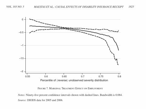
the predicted probability of SSDI receipt. Specifically, we regress initial allowance decisions on indicators for type of impairment, age group, decision month, and DDS, as well as a measure of average prior earnings, and construct the residual, Z, which by construction is orthogonal to the case mix controls and varies systemati-cally only with EXALLOW. Then we estimate a probit of ultimate SSDI receipt on the residualized Z. This is our measure of the predicted probability of SSDI receipt, P(Z ). Next we estimate a local quadratic regression of employment on predicted SSDI receipt and compute the numerical derivative of this function to estimate ∂E[ y]/∂P(Z ).

Figure 7 shows the MTE as a function of unobserved severity, where severity is reverse ordered and measured in percentiles (see definition of u in Section IVA), along with boot-strapped 95 percent confidence intervals. Applicants on the margin for an examiner with a predicted SSDI receipt rate of 65 percent (the mean rate) are in the sixty-fifth percentile of the unobserved (reverse) severity distribution. That is, they have an impairment that is less severe than 65 percent of applicants, and more severe than 35 percent of applicants. Since we estimate that 57 percent of applicants are always takers (that is, they would receive SSDI benefits regardless of initial examiner assignment), the MTE is not identified for applicants on the margin of SSDI receipt rates less than 57 percent. Similarly, the MTE is not identified for applicants on the margin of SSDI receipt rates greater than 80 percent (= 57 + 23, the fraction of marginal applicants). As a result, we are only able to trace the MTE for applicants between the fifty-seventh and eightieth percentiles of the unobserved (reverse) severity distribution (or the twentieth to forty-third percentiles of the actual unobserved severity distribution s). The estimates become imprecise at the more extreme ends of the distribution since there are relatively small numbers of examiners with margins at these points.

–2

–1.5

–1

–0.5

0

0.55 0.6 0.65 0.7 0.75 0.8

Percentile of (reverse) unobserved severity distribution

Figure 7. Marginal Treatment Effect on Employment

Notes: Ninety-five percent confidence intervals shown with dashed lines. Bandwidth is 0.084.

Source: DIODS data for 2005 and 2006.

Effect of DI Processing Time: Autor et al. 2013

DI requires a lengthy application process and 5 months out of the laborforce ⇒ Process takes 10 months on averageBeing out of the labor force for 10 months could hurt future job prospects⇒ Could partly explain why DI rejected applicants work so little ⇒ DIcould have higher negative effects [Parsons 1991 reply to Bound]Autor et al. 2013 test this using (quasi-random) variation in DI applicationsprocessing time due to backlogFind that 1 sd processing time delay (2.4 month) reduces employment rateby 1 point (3.2%) in years 2-4 for denied applicants⇒ DI processing time reduces LFP of denied applicants by 4.1 points [8%](significant but not super large)

61 69

DI and Unemployment: Autor and Duggan QJE’03

DI claims raise in recessions (as partly disabled workers have less workingoptions) ⇒ Reduces unemployment rate (DI recipients outside labor force)and labor force participationTest this hypothesis using cross-state variation in employment shocks(using industry mix Bartik’s instrument) [e.g., car industry shock createsemployment shock in Michigan]Negative employment shocks do increase DI applications and reduce thesize of labor force (workers+job seekers)DI keeps beneficiaries outside labor force permanently and is an inefficientsubstitute to temporary unemployment insurance benefits

62 69

Coefficient = 0.849, se = 0.164 t = 5.188

6

4

2

0

2

4

6

8

WY

ALAR

AK

WV

MS

MESC

KS

ND

GALA

KY

TNNC

OK

MTSD

UT

NVTXIDNE

WAIA

IN

MO

PAVA

NM

HIOR

DE

AZVT

CAWI

NY

MD

FL

ILCOOH

NJ

MI

MN

CTMANH

RI

8 6 4 2 0 2 4 6 8

Employment Shocks and DI Applications: 19931998

E[D

I App

s/P

op |

X]

E[Change in Employment/Pop | X]

Source: Autor and Duggan 2003


REFERENCES

Aguiar, M. and E. Hurst “Consumption vs. Expenditure”, Journal of PoliticalEconomy, Vol. 113, 2005, 919-948. (web)Attanasio, O. and A. Brugiavinni “Social Security and Household’s Saving”,Quarterly Journal of Economics, Vol 118, 2003, 1499-1521. (web)Attanasio, O. and S. Rohwedder “Pension Wealth and Household Saving: Evidencefrom Pension Reforms in the United Kingdom”, American Economic Review, Vol 93,2003, 1121-1157. (web)Autor, David H., and Mark G. Duggan. 2003. “The Rise in the Disability Rolls andthe Decline in Unemployment.” Quarterly Journal of Economics, 118(1): 157?205.(web)Autor, David, Nicole Maestas, Kathleen Mullen, Alexander Strand “Does DelayCause Decay? The Effect of Administrative Decision Time on the Labor Force

63 69

http://www.jstor.org/stable/pdfplus/10.1086/491590.pdf

http://links.jstor.org/stable/pdfplus/25053931.pdf


http://www.jstor.org/stable/pdfplus/25053901.pdf

Participation and Earnings of Disability Applicants”, working paper 2013(preliminary) (web)Barro, R. and G. MacDonald “Social Security and Consumer Spending in anInternational Cross Section”, Journal of Public Economics, Vol. 11, 1979, 275-289.(web)Bernheim, D., J. Skinner, and S. Weinberg, “What Accounts for the Variation inRetirement Wealth Among U.S. Households?”, American Economic Review, Vol.91, 2001, 832-857. (web)

Bound, John “The Health and Earnings of Rejected Disability InsuranceApplicants,” American Economic Review 79 (1989), 482-503. (web)

Bound, John “The Health and Earnings of Rejected Disability Insurance Applicants:Reply,” American Economic Review 81 (December 1991), 1427-1434. (web)Bound, John and Richard V. Burkhauser “Economic analysis of transfer programstargeted on people with disabilities,” In: Orley C. Ashenfelter and David Card,Editor(s), Handbook of Labor Economics, Elsevier, 1999, Volume 3, Part C,3417-3528. (web)

64 69

http://elsa.berkeley.edu/~saez/course/autormaestasetal13DI.pdf

http://elsa.berkeley.edu/~saez/course/Barro and MacDonald_JPubE(1979).pdf




http://elsa.berkeley.edu/~saez/course/bound-burkhauserHLE99.pdf

Brown, K. “The Link between Pensions and Retirement Timing: Lessons fromCalifornia Teachers”, Journal of Public Economics, 98, 2013, 1–14. 2007 (web)Chetty, Raj, John Friedman, Soren Leth-Petersen, Torben Nielsen, and Tore Olsen“Active vs. Passive Decisions and Crowd-out in Retirement Savings Accounts:Evidence from Denmark.” forthcoming Quarterly Journal of Economics 2014 (web)Diamond, P. “National Debt in a Neoclassical Growth Model”, American EconomicReview, Vol. 55, 1965, 1126-1150. (web)Diamond, P. “A Framework for Social Security Analysis”, Journal of PublicEconomics, Vol. 8, 1977, 275-298. (web)Diamond, P. and J. Mirrlees, “A Model of Social Insurance with VariableRetirement,” Journal of Public Economics, (1978) 295-336 (web)Diamond, P. and E. Sheshinski, “Economic Aspects of Optimal Disability Benefits,”Journal of Public Economics 57 (1995), 1-24. (web)Feldstein, M. “Social Security, Induced Retirement and Aggregate CapitalFormation”, Journal of Political Economy, Vol. 82, 1974, 905-926. (web)

65 69

http://elsa.berkeley.edu/~saez/course/brown_jpube13.pdf

http://www.nber.org/papers/w18565


http://elsa.berkeley.edu/~saez/course/Diamond_JPubE(1977).pdf

http://elsa.berkeley.edu/~saez/course/diamond-mirrleesJPubE78retirement.pdf

http://elsa.berkeley.edu/~saez/course/diamond-sheshinskiJpubE95DI-benefits.pdf


Feldstein, M. and J. Liebman “Social Security” in A. Auerbach and M. Feldstein,Handbook of Public Economics, Sections 1-5. (web)Feldstein, M. and A. Pellechio “Social Security and Household WealthAccumulation: New Microeconometric Evidence”, The Review of Economics andStatistics, Vol. 61, 1979, 361-368 (web)Friedberg, L. “The Labor Supply Effects of the Social Security Earnings Test”,Review of Economics and Statistics, Vol. 82, 2000, 48-63. (web)Gelber, Alex, Damon Jones, and Dan Sacks “Earnings Adjustment Frictions:Evidence from the Social Security Earnings Test”, Working paper 2013 (web)J. Gruber, “Disability Insurance Benefits and the Labor Supply of Older Persons,”Journal of Political Economy, 108(6), 2000. (web)Gruber, J. and D. Wise (editors) Social Security and Retirement Around theWorld. Chicago: University of Chicago Press, 1999 (book online) (IntroductionChapter is required reading) (web)

66 69

http://elsa.berkeley.edu/~saez/course/Feldstein and Liebman_Handbook.pdf



http://elsa.berkeley.edu/~saez/course/gelber-jones-sacks13.pdf

http://www.jstor.org/stable/pdfplus/10.1086/317682.pdf

http://www.nber.org/books/grub99-1

http://elsa.berkeley.edu/~saez/course/gruber-wiseNBER99ch1.pdf

Gruber, J. and D. Wise (editors) Social Security Programs and Retirement Aroundthe World: Micro Estimation. Chicago, University of Chicago Press: 2004. (bookonline)Gruber, J. and D. Wise (editors) Social Security Programs and Retirement Aroundthe World: The Relationship to Youth Employment. Chicago: University of ChicagoPress, 2010.Hamermesh, D. “Consumption During Retirement: The Missing Link in theLife-Cycle Hypothesis”, Review of Economics and Statistics, Vol. 66, 1984, 1-7.(web)Krueger, Alan B. and Jorn-Steffen Pischke “The Effect of Social Security on LaborSupply: A Cohort Analysis of the Notch Generation”, Journal of Labor Economics,10(4), 1992, 412-437. (web)Leimer, R. and D. Lesnoy “Social Security and Private Saving: New Time-SeriesEvidence”, The Journal of Political Economy, Vol. 90, 1982, 606-629. (web)Maestas, Nicole, Kathleen Mullen and Alexander Strand “Does DisabilityInsurance Receipt Discourage Work? Using Examiner Assignment to Estimate

67 69






Causal Effects of SSDI Receipt”, American Economic Review, 103(5), 2013,1797-1829. (web)

Manoli, Day and Andrea Weber, “Nonparametric Evidence of the Effects ofFinancial Incentives on Retirement Decisions,” NBER Working Paper No. 17320,2011 (web)Manoli, Day and Andrea Weber, “Labor Market Effects of the Early RetirementAge”, working paper in preparation, 2013 (web)

Page, B. “Social Security and Private Saving: A Review of the Empirical Evidence”,Congressional Budget Office, 1998 (web)Parsons, Donald “The Decline of Male Labor Force Participation,” Journal ofPolitical Economy 88 (February 1980), 117-134. (web)Parsons, Donald, “The Health and Earnings of Rejected Disability InsuranceApplicants: Comment,” American Economic Review 81 (December 1991),1419-1426. (web)Samuelson, P. “An Exact Consumption Loan Model of Interest With or Without theSocial Contrivance of Money”, Journal of Political Economy, Vol. 66, 1958. (web)

68 69

http://elsa.berkeley.edu/~saez/course/maestas-mullen-strandAER13.pdf

http://www.nber.org/papers/w17320.pdf

http://elsa.berkeley.edu/~saez/course/manoli-weber13ERAframes.pdf

http://elsa.berkeley.edu/~saez/course/pageCBO98.pdf




Scholz, J., A. Seshadri and S. Khitatrakun “Are Americans Saving “Optimally” forRetirement?”, Journal of Political Economy, Vol. 114, 2006, 607-643. (web)Social Security Administration Annual Statistical Report on the Social SecurityDisability Insurance Program. (web)Smetters, K. “Is the Social Security Trust Fund a Store of Value?”, AmericanEconomic Review, Vol. 94, 2004, 176-181. (web)

Von Wachter, Till, Jae Song. and Joyce Manchester, “Trends in Employment andEarnings of Allowed and Rejected Social Security Disability Insurance Applicants”American Economic Review, 2011, Vol. 101 No. 7, 3308-29. (web)

69 69


http://www.ssa.gov/policy/docs/statcomps/di_asr/


http://elsa.berkeley.edu/~saez/course/vonwachterAER-DI.pdf

stefanie stantcheva fall 2016 - harvard university

Documents