NBER WORKING PAPER SERIES

TAXATION AND INNOVATION IN THE 20TH CENTURY

Ufuk AkcigitJohn GrigsbyTom Nicholas

Stefanie Stantcheva

Working Paper 24982http://www.nber.org/papers/w24982

NATIONAL BUREAU OF ECONOMIC RESEARCH1050 Massachusetts Avenue

Cambridge, MA 02138September 2018, Revised October 2018

We thank Julie Cullen, Jim Hines, Henrik Kleven, Jim Poterba, Juan Carlos Suarez Serrato, Joel Slemrod, Ugo Troiano, Danny Yagan, Owen Zidar, Gabriel Zucman, Eric Zwick and seminar participants at UC San Diego, Duke Fuqua, Michigan, and NYU for comments and suggestions. We are deeply indebted to Jon Bakija for sharing his state-level personal income tax calculator. Akcigit acknowledges financial support from the NSF under Grant CAREER 1654719 and Sloan Foundation G-2018-11071. Nicholas acknowledges support from the Division of Research and Faculty Development at Harvard Business School. Stantcheva acknowledges support from the NSF under Grant CAREER 1654517. We thank Helen Ho, Rafael Jimenez, Raphael Raux, and Simeng Zeng for excellent research assistance. The views expressed herein are those of the authors and do not necessarily reflect the views of the National Bureau of Economic Research.

NBER working papers are circulated for discussion and comment purposes. They have not been peer-reviewed or been subject to the review by the NBER Board of Directors that accompanies official NBER publications.

© 2018 by Ufuk Akcigit, John Grigsby, Tom Nicholas, and Stefanie Stantcheva. All rights reserved. Short sections of text, not to exceed two paragraphs, may be quoted without explicit permission provided that full credit, including © notice, is given to the source.

Taxation and Innovation in the 20th CenturyUfuk Akcigit, John Grigsby, Tom Nicholas, and Stefanie Stantcheva NBER Working Paper No. 24982September 2018, Revised October 2018JEL No. H24,H25,H31,J61,O31,O32,O33

ABSTRACT

This paper studies the effect of corporate and personal taxes on innovation in the United States over the twentieth century. We use three new datasets: a panel of the universe of inventors who patent since 1920; a dataset of the employment, location and patents of firms active in R&D since 1921; and a historical state-level corporate tax database since 1900, which we link to an existing database on state-level personal income taxes. Our analysis focuses on the impact of taxes on individual inventors and firms (the micro level) and on states over time (the macro level). We propose several identification strategies, all of which yield consistent results: i) OLS with fixed effects, including inventor and state-times-year fixed effects, which make use of differences between tax brackets within a state-year cell and which absorb heterogeneity and contemporaneous changes in economic conditions; ii) an instrumental variable approach, which predicts changes in an individual or firm's total tax rate with changes in the federal tax rate only; iii) event studies, synthetic cohort case studies, and a border county strategy, which exploits tax variation across neighboring counties in different states. We find that taxes matter for innovation: higher personal and corporate income taxes negatively affect the quantity and quality of inventive activity and shift its location at the macro and micro levels. At the macro level, cross-state spillovers or business-stealing from one state to another are important, but do not account for all of the effect. Agglomeration effects from local innovation clusters tend to weaken responsiveness to taxation. Corporate inventors respond more strongly to taxes than their non-corporate counterparts.

Ufuk Akcigit Department of Economics University of Chicago 1126 East 59th Street Saieh Hall, Office 403 Chicago, IL 60637and NBERuakcigit@uchicago.edu

John Grigsby Department of Economics University of Chicago 1160 East 58th Street Chicago, IL 60637 jgrigsby@uchicago.edu

Tom NicholasHarvard Business School Soldiers FieldBoston, MA 02163 tnicholas@hbs.edu

Stefanie Stantcheva Department of Economics Littauer Center 232 Harvard University Cambridge, MA 02138 and NBERsstantcheva@fas.harvard.edu

“On the one hand, taxation is an essential attribute of commercial society... on the other hand, it

is almost inevitably ... an injury to the productive process.”

Schumpeter, Capitalism, Socialism, and Democracy (1942), p. 198.

1 Introduction

Major reform to the U.S. tax code under the 2017 Tax Cuts and Jobs Act has renewed interest in

the long-standing question – do taxes affect innovation? If innovation is the result of intentional

effort and taxes reduce the expected net return from it, the answer to this question should be yes.

Yet, when we think of path-breaking superstar inventors from history such as Wallace Carothers

(DuPont), Edwin Land (Polaroid), or William Shockley (Bell Labs and Shockley Semiconductor)

we often imagine hard-working and driven scientists, who ignore financial incentives and merely

seek intellectual achievement. More generally, if taxes affect the amount of innovation, do they also

affect the quality of the innovations produced? Do they affect where inventors decide to locate and

what firms they work for? Do they affect where companies allocate R&D resources and how many

researchers they employ?

Answers to these questions, while crucial to a clearer understanding of one of the most vexing

current public policy issues, have remained elusive due to a paucity of empirical evidence. In fact, in

the absence of systematic data, ambivalence towards tax policy may stem from a reliance on isolated

cases or anecdotes to confirm or reject particular viewpoints. The gap in our knowledge is especially

large when trying to understand the impact of tax policy on technological development over the

long-run. Although the United States experienced major changes in its tax code throughout the

twentieth century, we currently do not know how these tax changes influenced innovation at either

the individual, corporate or state levels.

In this paper, we bridge the data gap and provide new evidence on the impact of taxation on

innovation. Our goal is to systematically analyze the effects of both personal and corporate income

taxation on inventors as well as on firms that do R&D over the 20th century. Lack of data has

precluded any prior analysis of these important effects.

Our analysis leverages three new datasets. First, we construct a panel dataset on inventors based

on digitized historical patent data since 1920. These panel data allows us to track inventors over

time and observe their innovations, citations, place of residence, technological fields, and the firm (if

any) to which they assigned their patents. Second, we build a dataset on firms’ R&D activities over

the twentieth century, specifically the number of laboratories operated and research employment.

These data were obtained from National Research Council (NRC) Surveys of Industrial Research

Laboratories of the United States (IRLUS) for the period 1921 to 1970. Third, we combine the

new inventor-level panel data and firm-level R&D data with a new dataset on historical state-level

corporate income taxes and a database on personal income tax rates.1 The corporate tax data were

1Personal income taxes provided by Jon Bakija, who constructs a large scale tax calculator program to model

2

compiled from a range of handbooks and reference-works.

We provide a conceptual framework to help motivate our analysis and interpret the various

effects of taxes on innovation that we identify. This framework has the following intuition. Consider

an innovation production function in which the quantity and quality of innovation result from costly

investments in research expenses and effort. Inventors can work for firms or be self-employed.

Personal and corporate income taxes affect the net return to innovation. Since innovation inputs

are costly, they exhibit elasticities to net returns, the magnitudes of which will depend on the

market environment. If inventors work for firms, for example, their compensation derives from

surplus sharing with the firm.2 As a result, both firms and their inventors could be responsive to

both personal and corporate income taxes. These effects, in turn, may reflect a mix of extensive

margin responses (inventors or firms moving across states, individuals making occupational choices,

and entering or exiting the labor market) and intensive margin responses (inventors choosing how

hard to work on their research, companies choosing how many employees to hire).

Our empirical analysis starts at the macro, state-level, moves to event studies of large reforms

and some salient case studies, and then to the micro-level of individual firms and inventors.3 Using

the long-run historical data we implement several distinct and complementary strategies to identify

the impact of taxes on innovation. First, we control for a detailed set of fixed effects, including state,

year and, at the individual-level, inventor fixed effects, plus individual or state-level time-varying

controls. These help to absorb unobserved heterogeneity. In addition, we exploit within-state-year

tax differentials between individuals in different tax brackets (e.g., the top tax bracket versus the

median one) and thus also include state × year fixed effects. These controls filter out other policy

variations or the effect of contemporaneous economic circumstances in the state. Second, at the

macro and micro levels, we use an instrumental variable approach which predicts the total tax

burden facing a firm or inventor – which is a composite of state and federal taxes – with changes

in the federal tax rate only, holding state taxes fixed at some past level. This provides variation

driven only by federal level changes so is plausibly exogenous to any individual state’s economic

conditions. Third, we use a border county strategy, which exploits tax variation across neighboring

counties that lie in different states. It can be used as a standalone to identify the impact of taxes

on innovation or in combination with our IV approach. Finally, we provide evidence using episodes

of sharp tax changes in an event study design, as well as case studies using a synthetic control

analysis.

We begin by describing patterns in innovation and taxation over the 20th century. We focus

on key facts in relation to inventors, making use of the new panel data to show where inventors

located over time, where firms’ R&D labs were placed, and trends exhibited by the time series of

patents, citations, and research lab employment. We then document central patterns in taxation on

federal and state personal income taxes from 1900 through 2016 (Bakija, 2017).2For empirical evidence on the surplus sharing between firms, entrepreneurs, workers and inventors see Aghion

et al. (2018) and Kline et al. (2017).3It is worth noting that we are interested in the effects of general taxation, i.e., corporate and personal income

taxation, not specifically in innovation focused policies such as R&D tax credits, although we do control for those.

3

personal and corporate income over the 20th century, focusing specifically on our newly constructed

corporate tax database.

Next we turn to macro state-level results. We use OLS to study the baseline relationship

between taxes and innovation, exploiting within-state tax changes over time, our instrumental

variable approach and the border county design. On the personal income tax side, we consider

average and marginal tax rates, both for the median income level and for top earners. Our corporate

tax measure is the top corporate tax rate. We find that personal and corporate income taxes have

significant effects at the state level on patents, citations (which are a well-established marker of the

quality of patents), inventors in the state, and the share of patents produced by firms as opposed

to individuals. We show that these effects cannot be fully accounted for by inventors moving across

state lines and therefore do not merely reflect “zero-sum” business-stealing of one state from other

states. Our instrumental variable estimation results and the border county strategy confirm the

OLS fixed effects findings.

We then turn to the micro-level, i.e., individual firms and inventors. In addition to many

detailed inventor-level (fixed and time-varying) controls, we are able to include state × year fixed

effects to control for other possible policies that may have occurred simultaneously with tax changes.

Hence, we exploit within state-year variation. We make use of the fact that inventors of different

productivities have different incomes and will therefore be subject to different tax brackets. We

also implement our aforementioned instrumental variable approach at the individual-level. Again,

we find that taxes have significant negative effects on the quantity and quality (as measured by

citations) of patents produced by inventors, including on the likelihood of producing a highly

successful patent (which gathers many citations). At the individual inventor level, the elasticity of

patents to the personal income tax is 0.6-0.7, and the elasticity of citations is 0.8-0.9.

Furthermore, we show that individual inventors are negatively affected by the corporate tax

rate, but less so than by personal income taxes. Corporate inventors are much more elastic to

personal and corporate income taxes than non-corporate inventors (individual “garage” inventors

operating outside the boundaries of firms), and are especially strongly elastic to the corporate tax

rate. We also show that an inventor is less sensitive to taxes when there is more agglomeration – i.e.,

more inventors in the same technological field in the state. At the individual firm-level, we find that

corporate taxes – and to a lesser extent, personal income taxes – have significant negative effects

on the level of patents, citations, and research workers employed in corporate R&D laboratories.

Finally, we estimate a location choice model, in which inventors can choose in which state to

reside, trading off state characteristics against the effective tax rate in each state, conditional on

state × year fixed effects. We find that inventors are significantly less likely to locate in states with

higher taxes. The elasticity to the net-of-tax rate of the number of inventors residing in a state is

0.11 for inventors who are from that state and 1.23 for inventors not from that state. Inventors

who work for companies are particularly elastic to taxes. Agglomeration effects appear to matter

for location as well: inventors are less sensitive to taxation in a potential destination state when

there is already more innovation in that state in their particular field of inventive activity. This

4

is also true if an inventor’s employer already has a record of innovation activity in that state. We

confirm that firms are responsive to corporate taxes when choosing where to locate by estimating

a location choice model at the individual R&D lab level.

Our main findings can therefore be summarized as follows. Taxation – in the form of both

personal income taxes and corporate income taxes – matters for innovation along the intensive and

extensive margins, and both at the micro and macro levels. Taxes affect the amount of innovation,

the quality of innovation, and the location of inventive activity. The effects are economically large

especially at the macro state-level, where cross-state spillovers and extensive margin location and

entry decisions compound the micro, individual-level elasticities. Not all the effects of taxes at the

macro-level are accounted for by cross-state business stealing or spillovers. Corporate inventors are

most sensitive to taxation; and positive agglomeration effects play an important role, perhaps in

offering a type of compensating differential for taxation.

As a final note, while our analysis focuses on the relationship between taxation and innovation,

our data and approach have much broader implications. We find that taxes have important effects

on intensive and extensive margin decisions, on the mobility of people and where inventors and

firms choose to locate. Any rigorous analysis of these kinds of effects – on any type of agents, not

just inventors – has been impossible due to a lack of long-run data.4 Our new inventor panel data,

which stretches back to the early twentieth century allows us to uniquely track individuals each

year. To the extent that innovation is the outcome of investment and effort, just like a range of

other important pursuits such as entrepreneurship, the magnitudes of the elasticities to taxation

we find at the micro and macro levels on the extensive and intensive margins can help us bound

the effects on other types of economic activities and agents.

1.1 Related Literature

A key advantage of our new historical datasets is that they provide an opportunity to analyze a

series of variations in taxes over time and states and to study the effects of taxation systematically.

In that sense, our work is related to the recent public economics literature endeavoring to build

detailed long-run datasets of important economic outcomes, such as Piketty and Zucman (2014)

and Saez and Zucman (2015) on wealth in the United States and other countries, and Smith, Yagan,

Zidar, and Zwick (2017) and Cooper et al. (2016) on who owns wealth and businesses.

Our work contributes to the abundant and growing literature on the empirical effects of personal

taxes – on income or wealth – using data from recent time periods. Often, the focus of this research

is on the taxable income elasticity (Gruber and Saez, 2002; Saez, Slemrod, and Giertz, 2012), but

many specific and varied margins have been shown to be affected by taxation. These include work

contracts set by companies (Chetty, Friedman, Olsen, and Pistaferri, 2011), the self-employed’s

4Butters and Lintner (1945) conducted an influential analysis of the impact of federal individual and corporatetaxes on the growth of small and large firms during the 1930s and early 1940s finding the effects were largely negative,especially the impact of corporate tax on the growth rate of larger firms. However, their evidence was based on onlyfive firm-level case histories and they did not explicitly address the relationship between taxation and innovation.

5

reported income (Kleven and Waseem, 2013; Saez, 2010), rent-seeking (Piketty et al., 2014), or

charitable contributions (Fack and Landais, 2010). Cullen and Gordon (2006, 2007) study the

effect of personal income taxes taxes and their progressivity on startup activity and risk-taking by

entrepreneurs. At the macro level, Zidar (2017) studies how tax changes for different income groups

affect aggregate economic activity, finding that employment growth is mostly caused by tax cuts

for lower-income groups, but that the impact of tax cuts for the top 10% on employment growth

is much smaller. Kleven, Jakobsen, Jakobsen, and Zucman (2018) undertake a rare study of the

effects of wealth taxes on wealth accumulation given that such data are difficult to find.

On the corporate tax side, several empirical studies examine the impact (or absence thereof)

of dividend tax cuts (Yagan, 2015; Chetty and Saez, 2005). Attention has focused on the effects of

corporate and personal income taxes on the shifting behavior and evasion (Gordon and Slemrod,

2000; Slemrod, 2007) by firms and individuals. Slemrod and Shobe (1989) consider the elasticity of

capital gains realizations while Poterba (1989) investigates the relationship between capital gains

taxation, U.S. venture capital activity and entrepreneurship. Mahon and Zwick (2017) study the

heterogeneous effects of taxes on investment behavior by firms. Auerbach, Hines, and Slemrod

(2007) provide an analysis of, and recommendations for, corporate taxation in the U.S..

Our work is also related to a number of studies using data from recent time periods to analyze

the effects of state-level business and corporate taxation. Suarez Serrato and Zidar (2016) study

the incidence of state corporate tax changes on firm owners, workers, and landowners using a

spatial equilibrium model and find that each of these groups bears, respectively, 40, 30-35, and

25-30 percent of the burden. Fajgelbaum, Morales, Suarez Serrato, and Zidar (2016) study the

misallocation costs of state-level taxation and find large welfare gains from eliminating spatial

dispersion in taxes. Giroud and Rauh (2017) use establishment-level data to estimate the effects

of state taxes on business activity (employment and the number of establishments).

Since we study the location choices of inventors and firms across states in response to taxation,

our paper contributes to a recent literature studying migration decisions. Kleven, Landais, Saez,

and Schultz (2014) find very high elasticities of the number of high income foreigners in Denmark

using a preferential tax scheme implemented by Denmark in 1992 that reduced top tax rates for 3

years.5 Kleven, Landais, and Saez (2013) study the migration of football players across European

clubs. Most closely related, Akcigit, Baslandze, and Stantcheva (2016) study the international

mobility of top inventors in response to top tax rates since the 1970s and find significant, but small

elasticities. Bakija and Slemrod (2004) use Federal Estate Tax returns to show that higher state

taxes on wealthy individuals only narrowly impacts migration across U.S. states.6 Moretti and

Wilson (2014) and Moretti and Wilson (2017) study the effects of state taxes on the migration of

star scientists across U.S. states and also find highly significant effects of taxes on migration.

5By contrast, Young and Varner (2011) study the effects of a change in the millionaire tax rate in New Jerseyon migration and find small elasticities. Young et al. (2016) consider the migration of millionaires in the U.S. usingadministrative data.

6Liebig, Puhani, and Sousa-Poza (2007) study mobility within Switzerland, across cantons and find small sensi-tivities to tax rates.

6

Turning to the innovation literature, in endogenous growth models (Romer, 1990; Aghion and

Howitt, 1992; Akcigit, 2017; Aghion et al., 2014) innovation is the central engine of growth. How

innovation is affected by taxation is a key question because of the many positive social spillovers

that innovation induces (Klenow and Rodriguez-Clare, 2005). In a new line of work, Jones (2018)

theoretically and quantitatively studies how to tax top incomes in a world of innovation and positive

externalities from ideas. The elasticities derived in our paper can help calibrate the optimal tax

formulas in his paper.

A related strand of this literature studies the effects of policies like R&D tax credits on innova-

tion. Bloom et al. (2002); Bloom and Griffith (2001) find a positive impact of these incentives on

the level of R&D intensity over both short and longer time horizons. On the other hand Goolsbee

(2003) and Goolsbee (1998) argue that R&D tax credits mostly push up workers’ wages. Using

a regression discontinuity design based around firm size cutoffs for R&D tax subsidies in the UK,

Dechezlepretre et al. (2016) find significant effects of subsidies on both R&D spending and patent-

ing. Some research has been undertaken on the recent issue of patent boxes, whereby intellectual

property is moved to corporate tax havens (Griffith et al., 2014; Alstadsæter et al., 2018).

Finally, our work is related to numerous papers studying the origins of innovation at the micro-

level. Recent contributions include Jones (2010) and Jones and Weinberg (2011), which show

the effect of inventor age, Jones et al. (2008), which focuses on collaborations of inventors across

universities, Wuchty, Jones, and Uzzi (2007), which considers the role of team production, and

Jones (2009) on the growing trend towards specialization. Aghion et al. (2017) study the social

origins and IQ of inventors in Finland. Bell et al. (2017) and Akcigit et al. (2017) study the

parental backgrounds of inventors in the U.S. on, respectively, modern data and historical data.

Our data allows us to extend this literature by considering the impact of taxation over a long time

period for a multitude of innovation outcomes (quantity, quality, and location) that arise from both

inventor-level and firm-level behavior.

The remainder of the paper is organized as follows. Section 2 describes the source datasets and

our data construction. In Section 3, we document historical patterns of innovation and taxation

over the 20th century. Section 4 presents our conceptual framework underlying the relationship

between taxation and innovation. Section 5 explains our macro state-level estimation strategies

and presents our results. Section 6 explains the identification strategies at the individual firm and

inventor levels and discusses our micro-level findings. Section 7 concludes with some thoughts about

the implications of our results and future research avenues.

2 Data Sources and Construction

In this section, we describe the sources for and the construction of our three new datasets. All the

variables constructed from the raw data and used in the figures and tables are defined sequentially

throughout the text. Appendix A.1 provides the definitions of all the variables used in full.

7

2.1 Historical Patent Data and Inventor Panel Data

The starting point of our inventor panel data are the digitized patent records since 1836 detailed

in Akcigit, Grigsby, and Nicholas (2017) (hereafter, AGN). These data contain information on

almost every patent granted by the United States Patent and Trademark Office (USPTO) since

1836, including the home address of the first named inventor on each patent, the application

year, and the patent’s technology class. Since 1920, the data additionally contain the name of

every inventor listed on the patent document, and the entity to which the patent was assigned, if

applicable. Furthermore, using information on the inventors’ name and location, AGN match these

patent records to decennial federal censuses, which provide additional demographic information on

inventors, and, crucially, their income levels in 1940. Throughout our analysis, we use a patent’s

application year rather than its year of eventual grant as this is the date closest to the actual

creation of the innovation.

The major contribution of the current paper relative to AGN is to transform these patent data

into an inventor-level panel dataset. To do so, we disambiguate the data using the machine learning

algorithm of Lai et al. (2014). The challenge of disambiguating inventor records – determining if two

inventors named “John Smith” are the same or not, for instance – may be expressed as a clustering

problem. Given a set of patent records, the researcher must ascribe some probability that the two

records originate from the same inventor. To do so, we use information on the inventor’s name and

location, as well as the patent’s technology class, set of coauthors on the patent, and assignee. It is

very likely that two records that share the same inventor name, technology class, and location were

originated by one inventor. However, it is less likely that two inventors, both named John Smith,

were the same individual if one built computer chips for IBM in New York and the other created

new packaging for Kraft foods in Illinois.

The full algorithm is described in Online Appendix OA.1. Table A1 summarizes the results

of our disambiguation algorithm and compares them with those of Lai et al. (2014). Our disam-

biguation algorithm produces 4.9 million unique inventors, in our dataset of 6.4 million patents.

Considering only patents granted to inventors based in the U.S., we observe 2.7 million inventors on

4.2 million patents. Finally, restricting attention to U.S. inventors in our principal sample period

of 1940 to 2000, we see 1.95 million inventors and 2.8 million patents.

We supplement these patent microdata with the full matrix of patent citations from 1947

through 2010, which we use to construct a measure of patent quality. Due to well-known challenges

in interpreting raw citation counts as patent quality, we adjust patents’ citation counts following

the quasi-structural procedure laid out in Hall et al. (2001). In brief, this approach assumes that

i) the shape of the citation lag function is independent of the patent’s total quality, and ii) this

lag function is stationary over time. Under these assumptions, one may adjust raw citation counts

so that the mean adjusted citation count is constant over time by estimating a simple log-linear

regression. Citations received from patents granted in periods with a lower-than-average citation

propensity will be over-weighted in the adjustment, as will the citation counts of patents granted

8

at the beginning and end of the period, which particularly suffer from the truncation of our sample

at 2010.7

2.2 R&D Lab Data

Our second new dataset consists of information on the R&D activities of firms in the U.S. since

1921 based on National Research Council (NRC) Surveys of Industrial Research Laboratories of the

United States (IRLUS). This is an extensive and well-documented source of R&D data covering

private and publicly-traded firms. For example, Mowery and Rosenberg (1989) wrote about the

rise of U.S. R&D based on the early surveys. Our contribution is to utilize information from all

the surveys. We hand-entered data on all firms included from the 1921, 1927, 1931, 1933, 1938,

1940, 1946, 1950, 1956, 1960, 1965 and 1970 IRLUS volumes.

The NRC was established in 1916 to advise the government on science and technology. Gov-

ernment officials wanted to know where laboratories and scientists were located during the First

World War, and R&D became a topic of policy interest due to the rise of in-house R&D during the

1920s. This momentum to collect data carried on for most of the twentieth century. To collect this

data, the NRC undertook direct correspondence surveys with firms and sent firms questionnaires.

The resulting IRLUS volumes contain the firm-level summary data responses. Figure 1 shows an

example entry about the Polaroid Corp. – the innovative Massachusetts-based instant photography

firm – and the type of information one can read in each record.

Our R&D data contains several research input-based measures: the total number of research

workers employed at each firm and the number and location of R&D labs for each firm. The data are

mostly at the firm-level, with limited breakdowns of aggregates at the establishment-level. There

are no innovation output-based measures per se in the IRLUS surveys. To obtain such output-

based measures, we hand-linked R&D firms listed in the IRLUS volumes to assignees in U.S. patent

records. The resulting dataset is analogous to the link between the NBER patent database and

firms in the Business Register of the Census Bureau for the post-1975 years. It thus provides a

valuable historical, long-run counterpart.

2.3 Historical Tax Data

Personal Income Tax Database. We use personal income taxes at both the state and federal

level provided by Jon Bakija. These data contain the statutory marginal tax rates and brackets

for each state from 1900 through 2014. The data on federal taxes come from the IRS Statistics

of Income Individual Income Tax Returns publication, while state tax data were collected from a

mix of state income tax forms, and state tax laws from the state’s “annotated statutes,” sourced

from the Lexis-Nexis legal research database, and the law libraries at Georgetown and Cornell

7See Akcigit et al. (2017) Appendix B.1 for a detailed description of the adjustment procedure for our historicaldata. Alternative specifications of the citation lag function did not qualitatively change our results.

9

Figure 1: Example entry from the IRLUS publications

Notes: The image shows an example entry from the NRC’s publications “Industrial Research Laboratories of theUnited States.” The data was hand-entered based on such entries for all the years available: 1921, 1927, 1931, 1933,1938, 1940, 1946, 1950, 1956, 1960, 1965 and 1970.

Universities. Bakija (2017) details the full set of tax rate sources, and attempts to verify their

veracity. We also make use of the tax calculator program provided by Bakija (2017), which models

the personal income taxes faced by individuals with income y in state s in year t, after incorporating

federal tax deductibility, and other considerations.

Corporate Income Tax Database. The third new dataset used in this project consists of

a state-level historical corporate income tax database covering approximately the period 1900-

2016. Historically, many states had indirect corporate taxes, such as franchise taxes, imposed on

corporations for the privilege of doing business in a state. In several states, statutes make direct

taxes unconstitutional and franchise taxes get around this problem. Some states have one or the

other, sometimes both, but companies only pay one.

Types of franchise taxes include taxes on net income (which are extremely similar to corporate

income taxes and which we consider as such), Business enterprise tax (in New Hampshire), Gross

receipts tax or commercial activity tax (which is the gross receipts tax in Ohio), Business and

occupation tax (West Virginia, Washington, or Ohio, sometimes different for different industries),

net worth/capital stock/asset value/shareholder equity combination taxes, or a value-added tax

(Michigan’s single business tax which is a franchise tax, not a sales tax). Over time, the share of

states with direct corporate income taxes rather than indirect taxes has increased (see Figure A7

which will be discussed in more detail below).

We collect all corporate income tax rates (brackets and rates, if applicable), net income franchise

taxes when applicable (since they are very similar to corporate income taxes), as well as any

10

temporary surtaxes and surcharges levied on net income. In addition, we have information on

whether a state adopts the same tax base as the federal government for the corporate tax and

whether federal corporate income taxes are state deductible. There are differences in the taxable

base across states which are almost impossible to capture in a tractable way for the empirical

analysis. We instead test that our results are all robust to excluding the set of large states which

have a taxable income base that is too different, namely, Michigan, Texas and Ohio. All our results

excluding these states are available on demand.

The corporate tax data is collected from a multitude of sources, including detailed State Tax

Handbooks and Legal Statutes. For example, we use HeinOnline Session Laws, HeinOnline State

Statutes, ProQuest Congressional, Commerce Clearing House (State Tax Handbooks, State Tax

Review), State Tax reports, Willis Report, Council of State Governments Book of States, and

National Tax Association Proceedings. These sources are described in greater detail in Online

Appendix OA.3.

3 Innovation and Taxation: Measurement and Descriptive Statis-

tics

3.1 Inventors

Table 1 provides some key summary statistics about inventors. The average inventor appears in

the patent data for 3 (not necessarily consecutive) years, but a top 5% inventor remains for 14

years and a top 1% inventor for 31 years. On average, inventors remain in the same state, but the

most mobile inventors appear in 3 states over their careers. The number of patents per inventor is

also highly skewed, ranging from 2.55 patents for the average inventor to 26 patents for a top 1%

inventor. Even more concentrated are citations, an often-used marker of quality of an innovation

(Hall et al., 2001; Trajtenberg, 1990). The total citations of a patent are all the citations ever

received by this patent, subject to the adjustment described in Section 2. The average inventor

receives 83.42 citations for his patents, but a top 1% inventor receives 1189.25 over the course of

his career, and gets up to 329 citations per year. Inventors also frequently work in multiple fields:

the average inventor has patents in close to 2 USPTO technology classes and a top 1% inventor in

14 classes.8

Figure 2 shows the geography of innovation since 1940, by depicting patents per 10,000 residents

at the state level for each decade (Appendix Figure A1 shows inventors per 10,000 residents). In all

our analysis, the year t of a patent will be counted as the application date. This ensures a shorter

time interval between a tax change and an innovation outcome and is most indicative of when an

innovation was actually created, as opposed to granted. The North East Coast, the Chicago area

8The United States Patent Classification (USPC) system is maintained primarily to facilitate the rapid retrievalof every patent filed in the United States. The principal approach to classification employed today classifies patentsbased on the art’s “proximate function.” Patent classes may be retroactively updated as new technologies arise. Weuse the 2006 classification throughout this paper.

11

and California appear as major hubs early on. Patents per capita do not increase monotonically

through time, and the 1970s recession can be observed here. In the 1990s and 2000s there is a large

increase in patents per capita everywhere and an expansion of innovation regions.

Figure 3 shows the share of corporate inventors and patents over time. Corporate patents are

those patents assigned to corporations. Corporate inventors are defined here as inventors who have

at least one corporate patent in their career. Both shares have fluctuated, but increased significantly

over time.

3.2 R&D Labs

Figure 4 shows maps of the location of R&D labs for each of the IRLUS survey years. R&D labs

in 1921 were few and almost exclusively located on the East Coast and in the Midwest. Over

time, labs spread West to populate parts of the Midwest and clusters of labs appear in California,

specifically Los Angeles and San Francisco. As labs became more numerous, several hubs appeared

in places like Pittsburgh, Cleveland and Detroit, and more generally the northeastern part of the

country where the U.S. “manufacturing belt” emerged (Krugman, 1991).

Overall, the 1930s witnessed one of the most innovative decades in American history, despite

the Great Depression (Field, 2003), while innovation in areas like radar detection and aviation was

spurred by the potentially transformative effects of heightened R&D investment during the Second

World War (Gordon, 2016). These changes are consistent with the historical context. Griliches

(1986) notes that corporate R&D activity peaked during the late 1960s, with R&D expenditures

relative to sales falling by about 38% between 1968 and 1979. From late 1969 through much of the

mid-1970s the United States experienced one of the most significant recessions in its history. In

the Appendix, Figure A2 shows some further trends in R&D labs’ operations over time, such as

the number of labs and patents, citations, and researchers per lab.

On the firm side, the share of firms with R&D labs which have at least one patent in a given

year is 22%. The median firm-year has 3 patents, conditional on having any, and the mean is 10.3.

The distribution is right-skewed with 1% of firm-years having more than 20 patents.9

3.3 Personal Income Taxes

We now turn to describing some key facts about personal and corporate income taxes over the 20th

century. Because the corporate income tax database is newly collected and crucial to the analysis,

we devote some extra space to discuss corporate tax patterns. This multitude of tax variations at

the state level is leveraged in our empirical analysis.

The number of states with a personal income tax increases sharply between 1920 and 1940,

stagnates until the 1970s, during which time a number of additional states adopted a personal

income tax, before the number flattens out towards the end of the time period. The first year

9Figure A3 depicts additional detailed statistics about the innovation behavior of firms; we summarize the mainfindings here.

12

of introduction is not necessarily reflective of the relevance of taxation for most, or even many,

individuals in the state.10 State taxes initially mostly applied to top earners. For this reason our

analysis will focus mostly on the post-1940 period.

Many states have progressive tax systems, even though they are typically much less progressive

than the Federal system. States with progressive taxes are California, New York, and New Jersey.

Some states instead have flat taxes, e.g., Connecticut, Massachusetts, and Illinois.

Construction of the Tax Measures. At the state level, there have not only been many personal

tax rate changes, but also many frequent tax bracket changes. Because of these frequent changes

in the tax brackets, for our macro analysis, we compute the total effective tax rates, combining

state plus federal liabilities that apply to a single person who is at i) the median income and ii)

the 90th percentile income of the national income distribution. Our tax measures, which focus on

the tax liability at a given (relative) point in the income distribution, take into account changes in

the tax brackets and thus measure the total impact on individuals at different parts of the income

distribution.11 We use Jon Bakija’s calculator, which takes into account special rules and deductions

and refer the reader to Bakija (2017) for more details. We compute the following marginal and

average tax rates, used throughout:

(i) the 90th percentile income MTR, (denoted by MTR90 for conciseness).

(ii) the 90th percentile income ATR, (denoted by ATR90)

(iii) the median income MTR, (denoted by MTR50)

(iv) the median income ATR, (denoted by ATR50).

We explain how we assign tax rates to each individual inventor in Section 6. Figure 6 shows the

evolution of the marginal tax rate at the median income level decade-by-decade and Figure 7 shows

the evolution of the marginal tax rate at the 90th income percentile. State tax rates have followed

very different trajectories – and have often also evolved differently from the federal tax rate.12

Key Tax Variation. Our empirical analysis makes use of the multitude of personal and corporate

income tax changes that have happened since 1940. Figure 5 depicts the percent of states with

a change in their statutory state-level taxes, the mean size of the change, and the magnitude of

the top 10th largest change for each year. Panel A considers the personal income tax. The share

of states changing their tax rate in any given year (depicted on the left vertical axis) oscillates

between 12-20% in the pre-1970s period and between 15 and 25% or even up to 40% in the post

1970s period. The average tax change size fluctuates around 3-4 percentage points. The top 10%

tax change varies dramatically from year to year, reaching levels as high as 17 percentage points.

10For the interested reader, we report these trends in personal tax rates in Appendix Figures A4 and A511The innovation measures are also sensitive to using statutory rates, but the interpretation of the elasticities is

much less clear given the frequent bracket changes.12To provide some more detail, Figure A6 illustrates the evolution of the top tax rate and the tax rate at the median

income for a few highly inventive states, namely, California, Illinois, New Jersey, New York and Pennsylvania.

13

3.4 Corporate Income Taxes

Our measure of state-level firm taxation will be the top corporate marginal tax rate because, unlike

personal income tax schedules, the state-levels corporate tax schedules most often simply have

a (relatively low) threshold of exemption below which the tax rate is zero and above which the

top corporate tax rate applies. Any non-small firm would be subject to the top tax rate and the

majority of innovative activity happens at large firms. Small highly innovative firms may not be

directly subject to the top tax rate; however if they are successful and forward-looking, they will be

subject to the top corporate tax rate given that the thresholds are low enough. If small innovating

firms are not forward looking at all, we would expect this to dampen our estimated elasticities to

the corporate tax. In our regression analysis, we compute the total tax rate, taking into account

the top federal corporate tax rate and state and federal tax deductibility rules.

Figure 8 shows the year in which corporate taxes were first introduced at the state level. Early

adopters were Hawaii (1902), Wisconsin (1913), West Virginia, Virginia, and Connecticut (1915),

as well as Montana and Missouri (1917). The latest adopters were Nevada and Michigan (1968),

Maine and Illinois (1969), New Hampshire (1970) and Ohio and Florida (1972).

Figure 9 shows the evolution of the top corporate tax rates in all states, decade by decade. A

few key facts stand out. The number of states with a corporate tax increases sharply and then

flattens completely after 1972. The mean non-zero state tax increases from around 3.5% in 1920

to close to 8% in the 1990s, and has declined slightly to above 7% since then. The top 10% states

ranked according to corporate tax levels each year saw their corporate tax rise from 2% in 1920 to

around 10% today. The lowest 25% states never had a tax rate above 4%. The median state had

a non-zero corporate tax only since the late 1930s and it hovers around 6% today.13 States have

had very different experiences with corporate taxes, which is an advantage for our analysis. For

instance, California and New York were one of the relatively early adopters of a corporate tax and

have followed similar patterns, with tax rates rising continuously before 1980, and experiencing

stagnating levels thereafter. New Jersey was one of the late adopters but quickly brought its tax

rate up to the same level as California and New York. Illinois also adopted a corporate tax quite

late and kept it at a low and stable rate of close to 5% over time.

Panel B of Figure 5 depicts the percent of states with a change in their top corporate tax rate,

the mean size of the change, and the magnitude of the top 10th largest change for each year. On

average, one out of every 6 or 7 states faces a change in the corporate tax in any given year; that

share was much higher at one out of five in the 1970s and 80s. The mean tax change fluctuates

around 1.5-2 percentage points, and the largest top 10% tax changes reach up to 6 percentage

points.

Apportionment Rules. We briefly discuss apportionment rules for multi-state firms and how

they affect our results. Before the Uniform Division of Income for Tax Purposes Act (UDITPA)

13The patterns summarized here, as well as the evolution of top corporate tax rates in a few select states, are alsoavailable in detail for the interested reader in Appendix Figure A7.

14

in 1957, different states had different ways of dealing with the taxation of multi-state companies.

Although not all states adopted it, the UDITPA made these apportionment and allocation rules

of the business income of multi-state companies more uniform, with a three-factor formula based

on equal weights to the shares of a corporation’s payroll, property, and sales in the state. In the

past twenty years, the weight on sales has started to increase, which should arguably decrease

the importance for a company of corporate income tax in states in which it has property and

employment (but a low share of its sales).

In our sample only around 6.5% of firms have an R&D lab in more than one state at a given

time; nevertheless firms may have tax nexus in other states even if they do not have R&D labs

there. We do not have information on the three factors entering the apportionment formulas for

the firms in our sample. Thus, we simply use the corporate income tax prevailing in the state

where the firm has its R&D lab, and, for the few firms with R&D labs in multiple states, we use

the average corporate tax weighted by the share of labs in that state.

The estimated effect in our regressions is likely to be a lower bound of the true effect of corporate

taxes because the measure of the corporate tax we use is exactly equal to the true tax rate facing

single-state firms (i.e., firms which have tax nexus only in one state), and positively correlated with,

but not exactly equal to the true tax rate facing multi-state firms. At one end of the spectrum,

if all the apportionment weight was on the sales factor, and no sales happened in the state where

the R&D labs are located, we should estimate a zero effect of corporate income taxes in that state.

At the opposite end, if firms have a nexus only in the state where their R&D lab is located, the

corporate tax of that state is the one that matters.14 In between, the higher the share of the firm’s

sales, property, and employment in the state where its R&D lab is located, the closer the estimated

effect of the corporate income tax should be to the true effect.

Other taxes: Discussion. Although not the focus of our paper, which concentrates on corporate

and personal income taxation, alternative methods of taxation exist as potential confounding fac-

tors, which may pollute our estimates if they are not adequately taken into account. Therefore, it

is worth considering how these alternative taxes may impact our proposed identification strategies.

Ordinary, non long-term capital gains are taxed as ordinary income and so are accounted for by our

personal income tax measures. Long-term capital gains are taxed at a reduced form at the Federal

level, which is captured by year fixed effects. In a few instances, states have special treatments

of long-term capital gains, which is captured by our state × year fixed effects.15 Dividends are

typically taxed as ordinary income at the Federal level and in most states; they are thus again

captured by our personal income tax measures. States’ sales taxes are absorbed by our state ×year fixed effects. In addition, our instrumental variable strategy results are robust to omitted

variables, not only taxes, and, as we will show below, yields very consistent results. We always

control for state-level R&D tax credits.

14Of course, when it comes to location decisions, as we will explore in Section 6, the tax rates of all states matter.15In any case, it is also not evident that the long-term capital gains rate is more relevant than the short-term one.

15

4 Conceptual Framework: Effects of Taxes on Innovation

What are the possible channels through which the taxation of personal and corporate income can

affect innovation by firms and individual inventors? We provide a very simple illustrative toy model.

A Toy Model of Innovation. Suppose that inventor i has decided to live in state s with personal

income tax rate τyis and corporate tax rate τ cs . y indexes personal income taxes; c indexes corporate

taxes.16 The inventor needs to choose how much effort ei to exert and how many resources ri (i.e.,

material innovation inputs, such as R&D expenses, lab space, machinery and equipment, etc.) to

devote to innovation. Effort has a disutility cost hi(ei) and resources cost m(ri). Inventors can

patent on their own, or can be employed by companies. If the innovation is developed within a

firm j, the firm also provides innovation inputs, denoted by Rj . In addition, each state has an

innovation infrastructure and economic policy framework, denoted by Xs which can improve the

productivity of the private inputs to innovation and/or shift the profits obtained from them.

The quantity k and quality q of the innovation produced depend positively on effort and re-

sources invested by the inventor, as well as by the firm (if the inventor is employed), and on the

state’s innovation policies and resources, with:

ki = k(ei, ri, Rj , Xs) qi = qi(ei, ri, Rj , Xs) (1)

If an inventor is self-employed, his innovation does not depend on the firm inputs Rj .

Inventors receive a private benefit bi from innovating, due to the “warm-glow” of being success-

ful, or from a “love for science.” bi is itself an increasing function of the quality and quantity of

innovation produced, with bi = bi(ki, qi). Let gi be the weight that inventor i puts on his private

benefit and (1− gi) the weight on the financial returns from an innovation.

A self-employed inventor can sell his innovation to a producer (e.g., a firm) or can himself start

producing a new marketable item based on it. His payoff depends on his innovation quality and the

policies and market structure in the state (including the intellectual property protection), which

we denote π(ki, qi, Xs). The inventor can incorporate as a firm or remain self-employed, which

means that the innovation can possibly be taxed in different tax bases. To allow for all possible

combinations, suppose that, in the case of inventor i, a share βci of that surplus is taxed in the

corporate tax base (if the inventor incorporates) and a share 1 − βci is taxed in the personal tax

base (if the inventor keeps being self-employed). Note that the share of the payoff that accrues to

the personal vs. corporate income base could also be endogenized in response to taxes to capture,

among others, income shifting responses.

The self-employed inventor’s total payoff is then:17

16The location itself is of course an endogenous choice.17For the exposition, R&D costs are not deductible. We discuss below that the larger the share of costs that is tax

deductible for firms and inventors, the smaller the empirical tax response of innovation will be.

16

V SEis = max

ei,ri

((1− gi)

[1− (1− βci )τyis − βci τ cs

]π(ki, qi, Xs) + gibi(ki, qi)− hi(ei)−m(ri)

)where ki and qi are functions of effort and resources as given by (1).

Inventors can also choose to be employed by firms. In the labor market of each state, firms open

one or several vacancies at a cost γj per vacancy for firm j, and inventors are matched to firms

to fill each of these vacancies. Jointly, inventors and firms produce a gross-of-tax surplus V (q, k)

that depends positively on the innovation quantity and quality produced by the match. Aghion

et al. (2018) and Kline et al. (2017) offer recent evidence on how the surplus from innovation is

shared between inventors, entrepreneurs/firms, and blue and white-collar workers. The surplus

thus produced is first taxed at the corporate tax τ cst. The firm pays resource costs Mj(Rj) to invest

in innovation. Imagine there is Nash bargaining between the firm and each worker with bargaining

weight α of the worker. Then the wage paid to the worker with outside option (from being a

self-employed inventor) V SEi is:

wi(q, k;V SEi ) = V SE

i + α[(1− τ cst)V (q, k)−Mj(Rj)− hi(ei)−m(ri)− V SE

i − γj]

and the firm’s payoff Wij from being matched to inventor i is:

Wij = maxRj

((1− α) ·

[(1− τ cst)V (q, k)−Mj(Rj)− hi(ei)−m(ri)− V SE

i − γj])

The value of an employed worker is:

V Eis = max

ei,ri

((1− gi)(1− τyis )wi(qi, ki;V

SEi ) + gibi(ki, qi)

)The inventor will choose to be self-employed if and only if V SE

is ≥ V Eis .

Response Margins to Taxation: Personal and corporate income taxes enter the payoffs of both

firms and inventors. Inventors and firms can respond to these taxes along the following margins:

(1) Innovation input choices: effort ei and resources ri in the case of inventors; material inputs

Rj and research employment for firms. Choices occur on the intensive and extensive margins.

(2) Occupational choices for inventors, i.e., whether to be self-employed or employed, or, more

broadly, whether to engage in innovation at all.

(3) Tax base choices, i.e., whether to incorporate or to sell the innovation, reflected in βci .

(4) Research employment, i.e., the number of vacancies to open.

(5) Location choice of both firms and inventors: the choice of the state s where to locate.

Effects of Taxes: Discussion. We can hypothesize the following effects of taxes:

(i) Personal and corporate income taxes can affect both firms and inventors, due to surplus

sharing and the possibility to shift the payoff from an innovation to either tax base.

17

(ii) Responses of innovation to taxation are shaped by technological parameters, such as the

elasticities of innovation quality and quantity to effort and resource costs by agents and firms.

For instance, it may be that quantity is very sensitive to inputs, but that quality is not. Does

one just “stumble” upon high-quality innovations or do they require consistent, intentional inputs?

Uncertainty in the returns to innovation can also affect the strength of these responses in the case

of risk-averse agents, as it can for other types of investments.

(iii) The elasticity to taxation depends on the extent to which innovation requires intentionally

directed inputs and how sensitive those inputs are to net returns. If ideas happen without any willful

input (such as for Newton sitting under a tree and discovering gravity from an apple falling), or

the inputs required to produce them are completely inelastic to net returns (as the stereotype of

the “mad and passionate scientist” would predict), then the elasticity of innovation to taxes would

be zero. If, to the contrary, innovation requires intentionally directed inputs and those inputs are

sensitive to net returns, we would expect stronger responses of innovation to taxes. The strength

of the response will also depend on how strongly innovators value the private warm-glow effect

relative to financial returns. Firms’ and inventors’ responses will be less pronounced the more

research inputs are tax deductible.18

(iv) Corporate and non-corporate inventors may exhibit different responses given their differ-

ential exposures to corporate and personal tax rates, as well as their motives for innovating and

their weight on private benefits vs. financial returns.19

(v) When it comes to location choices, inventors may choose to trade-off a higher tax in favor

of other factors – for instance they may prefer to remain in a place with more inventors in general,

or more inventors in one’s own technology field to benefit from the associated amenities. Such

“agglomeration” effects may enter the production function directly through Xs and improve the

productivity of any given innovation input. We will study how our tax elasticity estimates vary

with “agglomeration.”

Dynamic Effects. Although this simple framework is static, the effects of taxes on innovation

can be dynamic. First, there may be a lag between changes in taxes and changes in innovation

outcomes, depending on how long the process from inputs to a finished innovation takes. Some

new innovation may simply require scaling up already existing inputs, which can happen very

rapidly, e.g., providing existing highly-skilled R&D employees with more funding to test additional

chemicals. Developing other innovations may require a much lengthier process of trial and error

or adjusting scarce inputs sluggishly, e.g., having to find highly-specialized researchers to hire. In

our benchmark analysis, we will thus use lagged tax rates and the application date of the patent to

measure outcomes (not the grant date, which comes later). We also allow for a three year window

18Effort investments are typically difficult to make fully tax-deductible. They can also be interpreted more broadlyas unobservable R&D inputs (for a discussion of R&D policies when there is asymmetric information and unobservableR&D investments, see Akcigit et al. (2016)).

19Furthermore, the sensitivity of an inventor’s wage to his innovation output depends on the bargaining structureand his bargaining weight. And the outcome of innovation at the firm-level depends on the joint inputs of firms andinventors, each of which react to taxes in a different way.

18

to measure individual-level innovation outcomes. The event study and several case studies (see

Section 5.5) explicitly look at the dynamic path of responses to taxes.

Innovation can also be forward looking because the initial investment may possibly pay off over

a longer period. The importance of forward-looking effects for tax responses depends on the pattern

of payoffs from the innovation, on whether a given tax change is considered to be short-lived or

more persistent, and on how people form their future expectations about tax rates based on current

tax rates. These are common issues for empirical studies of taxation related to forward-looking

investments. We would expect lower elasticities to current or lagged tax rates if innovation payoffs

are more back-loaded, if agents are more forward-looking, and if future and current tax rates are

less correlated .

Micro and Macro Elasticities. At the individual inventor level, some of the response margins

are directly observable, such as his location choice. Some outcomes of interest, however, will be

the result of several responses. For instance, we will look at the number of patents and the number

of citations at the individual inventor level. The total response measured can be the result of an

inventor changing his work effort (the primitive “labor supply” elasticity) or investment of resources,

or shifting between the corporate and personal tax bases. Thus, our micro-elasticities capture the

reduced-form individual-level responses.20

For macro, state-level outcomes, the total responses measured are the result of both firms’

and inventors’ individual-level responses, and across all the margins, intensive and extensive. In

addition, they also capture movements across states, cross-state spillovers, or business-stealing. We

offer suggestive evidence below that the state-level tax effects are not purely zero-sum.

To sum up, there are several margins through which firms and individual inventors (corporate,

non corporate, or a mix of the two) can be affected by both personal and corporate income taxes.

Their decision margins concern how much innovation inputs to supply, where to locate and whether

to participate in the innovation process at all. These theoretical effects should be observable in the

data with respect to the quantity, quality, and location of innovation. We now turn to testing the

magnitudes of these margins empirically.

5 The Macro Effects of Taxation

We begin with the effects of personal and corporate taxes at the macro, state level over the period

1940-2000. Let us denote by τ cst the corporate tax in state s year t and τyjst the personal income

tax at income percentile j in state s in year t. Let the corresponding federal level tax rates be τ cft

20It is worth noting that some caution is needed to extrapolate the individual-level responses in order to understandwhat may happen if there is a federal tax change. A nation-wide tax change may create further general equilibriumramifications. Nevertheless, given the detailed controls in our regressions, the estimated elasticities are informativeabout people’s responses to tax changes or the net returns in general.

19

and τyjft . We focus on two income percentiles: the 90th percentile and the median.21 Heuristically,

ignoring the many complications of the tax code, the total tax rate on individuals with income at

the jth percentile who live in state s at time t is denoted by T yjst and is equal to:

T yjst = τyjft (1− τyjst ) + τyjst −D

yst · τ

yjst τ

yjft (2)

where Dyst is a dummy equal to 1 if the personal income tax paid at the federal level is deductible

from the state tax base in state s in year t. In practice, several states allow for the deductibility

of federal taxes, and this has changed over time. Some key examples include California and New

York throughout the 1940-2000 period, and Pennsylvania since 1971. Similarly, the total tax rate

of a firm in state s in year t is:

T cst = τ cft(1− τ cst) + τ cst −Dc

st · τ cstτ cft (3)

In this section, we estimate the following type of equations:

Yst = α+ βyTyjst−1 + βcT

cst−1 + γXst + δt + δs + εst (4)

where Yst is some innovation outcome in state s in year t (see below). T yjst−1 is the lagged personal

income tax rate (average or marginal) for income group j (median or 90th percentile) in state s

and T cst−1 is the lagged top corporate tax rate. δt and δs are sets of year and state fixed effects. Xst

are time-varying state-level controls, namely, lagged population density, real GDP per capita, and

R&D tax credits, intended to capture the effect of time-varying urbanization, economic activity,

and R&D incentive programs. Throughout, we weight each state by its population.22 βy and βc

are consistent estimates of the reduced-form state-level effects of personal and corporate taxes if,

conditional on the state and year fixed effects and the controls, changes in state-level tax rates

are not correlated with other policies or economic forces that affect innovation. We will relax this

assumption using two other identification strategies below.

Innovation outcomes: The innovation outcomes Yst at the state-year level are as follows: (i) The

quantity of innovation, as measured by the (log) number of patents produced during that year in

the state; (ii) The total quality of innovation, as measured by the (log) number of total forward

citations ever received by the patents produced in the state that year (subject to the adjustment

described in Section 2); (iii) The (log) number of inventors living in the state that year; (iv) The

share of innovation undertaken by companies, as captured by the share of patents assigned i.e.,

inventors transferring patents to their employer through assignment rights.

As explained in Section 4, at the macro level, the effects of taxes on the innovation outcomes

21Following the reasoning from Section 3.3, we use tax rates at fixed income percentiles, rather than tax rates infixed brackets, because tax brackets at the state level have changed extensively over time.

22In unreported results available on demand, we find a qualitatively similar effects of taxes on innovation per capita- higher taxes for both individuals and corporates tend to reduce per capita patents, citations, and inventors.

20

are the total effects on firms and inventors and the mix intensive and extensive margin responses.

Thus, we consider marginal tax rates, which matter for intensive margin responses, and average

tax rates, which matter for extensive margin responses.23

5.1 OLS Results

Panel A of Table 2 shows the estimates from the state-level regressions in (4). Each column

represents a different innovation outcome Yst at the state-year level, in the order (i)-(iv) listed

above.

Each row shows the coefficients from separate regressions of the format in (4), where different

tax measures are used for personal tax rates. Rows 2 to 5 use, respectively, the marginal tax rate

at the 90th percentile income (MTR90), the marginal tax rate at the median income (MTR50), the

average tax rate at the 90th percentile income (ATR90), and at the median income (ATR50). All

regressions control for the lagged top corporate tax rate T cst−1 but the coefficients on the corporate

tax are almost identical in every regression to the one in the first row, where MTR90 is used as the

personal tax measure. We thus report it only once.

All the tax measures – personal and corporate – are significantly correlated with lower patent

counts at the state level. A one percentage point increase in MTR90 is associated with approx-

imately a 4% decline in patents, citations, and inventors. The effects of the MTR50 are similar,

but larger. The effects of average personal tax rates are larger still. A one percentage increase in

ATR90 is associated with a roughly 6-6.3% decline in patents, citations, and inventors. For ATR50,

the effects fluctuate around 10% for patents, citations, and inventors.24 The macro elasticities to

marginal tax rates implied by these coefficients fluctuate around 2 (for the MTR90) and 3.4 (for

the MTR50) for patents, inventors, and citations.

These elasticities are large because they are state-level, macro elasticities, which incorporate

spillover effects and cross-state shifting responses, as well as the full mix of extensive and intensive

margin responses by firms and inventors. They are consistent with the typically large macro-level

elasticities estimated for other variables such as GDP. Naturally, the elasticities at the individual

micro level below – as well as the location elasticities – are much smaller.

A one percentage point higher top corporate tax rate leads to around 6.3% fewer patents, 5.9%

fewer citations, and 5.1% fewer inventors. The implied macro elasticities are, respectively, 3.5, 3,

and 2.5. It is worth noting that if we look at superstar inventors only, defined as inventors in the

top 5% of the patent count distribution in year t, where patent count at time t is an inventor’s total

patents up to and including t − 1, they are similarly negatively affected by taxes. Thus, higher

taxes have negative effects on the presence of the highest quality inventors as well.

23In taxation models with spillovers, this distinction is not clear-cut, which further justifies the need to considerboth types of taxes.

24Given that citations and patents – i.e., patent quality and quantity – seem to react very similarly to taxation atthe macro levels, average quality as measured by citations per patent exhibits a mildly negative, but not systematicallysignificant response to taxes.

21

The share of patents assigned to companies appears to be very sensitive to the corporate tax

rate, which is to be expected based on the framework in Section 4. A one percentage point increase

in the top corporate tax rate is associated with close to 1.2 percentage points fewer patents assigned

to companies. In fact, higher corporate taxes are associated with fewer non-corporate patents too,

but non-corporate patents are more responsive, so that the share assigned is lower overall. The

share assigned is also negatively related to the personal income tax rate. This is perfectly in line

with our finding at the micro level in Section 6 that corporate inventors are systematically more

sensitive to both corporate and personal taxes.

For robustness, Panel A of Appendix Table A2 replicates these results using only statutory

state-level taxes (not effective taxes); the effects are similar. One potential concern is that the

effects are sensitive to large, highly-innovative states such as California. Panel B, which drops

California from the analysis, shows that this is not the case.

5.2 Instrumental Variable Strategy using Federal Tax Changes

Our OLS estimates may be biased if states set their taxes in response to their economic conditions

or contemporaneously with other economic policies that can also affect innovation. We can address

this concern with an instrumental variable strategy that exploits changes in total personal and

corporate tax burdens that are not driven by changes in state taxes, but rather exclusively driven

by federal tax changes.

Our instrument is similar in spirit to the predicted tax burden in Gruber and Saez (2002) or

the predicted eligibility in Currie and Gruber (1996). Specifically, the instrument used for the

personal or corporate tax in state s at year t is the tax that would apply if the state-level personal

or corporate tax rate did not change since year t−k (where k is allowed to vary for robustness), but

federal taxes were changing as they are in reality. Changes in the predicted tax are therefore driven

purely by federal tax changes, which are likely exogenous to any given state’s economic conditions

and other policies. The impact of federal tax changes varies by state and by income group based on

the level of its state taxes (because of the state tax deductibility from federal taxable income) and

on whether the state allows for federal tax deductibility. The specification always includes state

and year fixed effects as well.

Using the same notation as above, the instrument for the personal income tax of income group

j in state s and year t, denoted by T yjst , can be written (heuristically) as:

T yjst = τyjft (1− τyjst−k) + τyjst−k −D

yst−k · τ

yjst−kτ

yjft (5)

where the actual state tax in year t is replaced by its lag τyjst−k at time t−k, and where we allow k to

vary for robustness (the benchmark has k = 5, results with other values for k are very similar and

available on demand). In practice, this instrument is calculated from the tax simulator, taking into

account many layers of complexity of the state and federal tax code, as is done for the actual tax

rate T yjst . Similarly, we instrument the corporate tax rate using the predicted tax burden holding

22

state taxes fixed at their level in year t− k (again, the benchmark is k = 5),

T cst = τ cft(1− τ cst−k) + τ cst−k −Dc

st−k · τ cst−kτ cft (6)

The results are presented in Panel B of Table 2. The IV estimates are highly significant and very

close to the OLS estimates, albeit slightly larger. One potential explanation for this is that states

are adjusting their tax rates in a counter-cyclical fashion, which would bias the OLS estimates

downwards.

5.3 Border Counties Strategy

As already explained, consistency of the OLS estimates requires that changes in state-level taxes

are not correlated with a state’s economic conditions. One way of alleviating this requirement

is to consider border counties, i.e., neighboring counties that lie in different states. Because such

counties are located next to each other, they are presumably subject to similar economic conditions

and shocks, but not to the same tax policies, since those are set at the state-level. Furthermore, we

can also alleviate the concern about state policies being set endogenously by combining the border

county strategy with the instrumental variable strategy, thus comparing innovation outcomes in

neighboring counties and shifting their total tax burdens using only federal-level variations.

We start by matching all inventors and patents to their counties and we restrict the sample to

neighboring counties across state lines. We then run the following modified version of (4):

∆Yit = βy∆T yjit−1 + βc∆T

cit−1 + γ∆Xit + δi + εit (7)

where i indexes a pair of border counties in two different states, δi is a pair fixed effect, and the ∆

operator takes the difference of any variable between the two border counties of a pair. Thus, ∆Yit

is the difference in innovation outcomes between the two counties; ∆T yjit−1 is the difference in lagged

personal tax measures for income group j and ∆T cit−1 is the difference in the lagged corporate tax

rates and Xit contains the same controls as above. We restrict attention to sufficiently large border

county pairs in which both counties have at least 6 patents in a given year, but the results are robust

to including even small counties. We again weight each county pair by its combined population.

Panel A of Table 3 shows the results of the estimation of (7) using OLS. The estimated effects

of personal and corporate income taxes are significantly negative and generally very comparable to

the benchmark macro results from Table 2.

To combine the border county strategy and our IV approach, we instrument the tax rate dif-

ferentials between the border counties with the difference in the instruments ∆T cit−1 and ∆T yj

it−1as defined in (5) and (6). The results are shown in Table A3 and the coefficients gravitate around

their values shown in either the border county OLS (Table 3) or the macro state IV results (Table

2) and are, if anything, even stronger.

Overall, the border county strategy, either using OLS or our instrumental variable specifica-

23

tion, also confirms that there are significant effects of personal and corporate taxes and that the

magnitudes are consistent with the ones found at the macro state-level.

5.4 Cross-State Spillovers and Business Stealing

The macro effects just discussed can be interpreted as the relevant reduced-form effects states

should take into account when considering whether to lower or raise their personal or corporate

income taxes, without retaliation from other states. Thus, they are of interest per se. These effects

may be partially driven by positive or negative spillovers on other states, due to business stealing

and to the possibility that factors and demand may shift across state lines. Although potentially

valuable to each individual state, these effects do not necessarily represent net extra value creation

in innovation when aggregated up to the federal level. To better understand these net effects, we

adopt two approaches.

First, as we will show in Section 6, inventors and firms do relocate in response to taxation and

this is an important margin of interest when thinking of the impact of taxes. Therefore, in Table

4, we replicate our core macro results (Panel A) and border county results (Panel B), but drop

all inventors who ever moved states. The magnitudes of the effects are only very slightly reduced.

Again, this estimation can be done using the IV strategy and yields very similar results (see Table

A3). Thus, to a first order, it appears that the effects of one state changing its taxes are not purely

driven by inventors moving across states.

Cross-state spillovers can also arise when other factors (not only inventors) or demand moves.

To test for this possibility, we can compare the estimated total border county effect (between the two

border counties of a pair) to the change in the same innovation outcome between the border county

that did not experience the tax change and the average county in its state. To be more precise,

denote the county with the tax changem and n the border county of the same pair, and k the average

county in the same state as n. Under the assumption that the difference in outcomes between the

border county n and the average county k in its state would have remained constant before and

after the tax change, the change in outcomes between these two counties measures the spillover

that occurs in n from the tax change in m. In principle, the double difference in outcomes between

m and n (which is the total border county effect measure above) and the difference between n and

k (the spillover effect) is a measure of the tax effect net of spillovers from, or to, the neighboring

county. Of course, there may also be spillovers to and from other states which we will not capture

and filter out with this method. Nevertheless, one may think that spillovers to the closest state

seem most likely in many cases and could be the largest.

The equation estimated is:

Ymt − Ykt = βy∆T yjit−1 + βc∆T

cit−1 + γ · [Xmt − Xkt] + δi + εit (8)

where i again indexes a pair of border counties in two different states, δi is a border pair fixed

effect. The left hand-side is the difference in innovation outcomes between the border county m

24

and the average county in the neighboring state (excluding the border county of the pair). ∆T yjit−1

and ∆T cit−1 are, as before the differences in lagged personal and corporate tax rates.25

Results. The results are shown in Panel B of Table 3. Overall, the net effects of taxes, even

filtering out the spillovers, are still consistently and systematically negative. Approximately, 50%

of the effects of the corporate tax on patents, citations, and inventors can be interpreted as a true

effect on net innovation, while the remaining 50% could be interpreted as spillovers across state

lines. There is heterogeneity in the spillovers by innovation outcomes though: the net effect on

inventors becomes insignificant; the effect on corporate patents is barely changed, suggesting there

are few spillovers on that margin. The MTR50 has much stronger spillovers than the MTR90,

perhaps because of lower substitutability or higher moving frictions in the high-skilled inventor

market. Spillovers seem to account for slightly more than 50% of the total effect of the MTR50

on patenting, citations, or inventors. Consistent with spillovers being driven by extensive margin

responses (such as factors relocating), it is the average tax rates that show the strongest spillover

effects. Almost 80% of the effects of the ATR50 disappear when filtering out spillovers to the

neighboring state. Just above 50% of the effects of the ATR90 on patents and inventors and 75%

of the effects on citations seem to be accounted for by spillovers. Citations seem to be particularly

prone to spillovers, perhaps because it is the highest quality research that is relocated.

Overall, this is suggestive evidence that there are significant spillovers across neighboring states

especially, but that they cannot explain the full effect of taxes. This is consistent with the significant

elasticities at the micro inventor and firm level we will describe in Section 6.

5.5 Event Studies: Large Tax Reforms

To study the dynamic effects of taxes and provide some clear-cut visual evidence, we implement an

event study analysis using large reforms that have happened over the course of the 20th Century. A

large tax change is defined to be in the top 10% of tax increases or in the top 10% of tax decreases

over the period 1940-2000. It corresponds to tax increases of at least 7 percentage points for the

personal income tax and 15 percentage points for the corporate tax and to tax decreases of at least

4 percentage points for the personal income tax and 9.3 percentage points for the corporate income

tax. For each such reform, we use the period of 4 years before and after each reform, for a total

time span of 9 years.26 We drop reforms which happen in the same time interval as other large

reforms. All tax changes are relabeled to be “tax increases.”

Figure 10 shows the results. Time t = 0 is the first calendar year during which the new tax

rate applies. We plot the coefficients on the time dummies relative to the year before the new

tax applies, i.e., year t = −1. The left column shows the effects of personal income tax reforms;

25Again, we can combine this estimation strategy with our instrumental variable approach, where, as in Section5.3, the difference in tax rates ∆T yj

it−1 and ∆T cit−1 can be instrumented by the difference in instruments, ∆T c

it−1 and

∆T yjit−1. Results are available on demand.

26The time span length is chosen to be as large as possible, while also avoiding too many overlapping reforms.

25

the right column shows the effects of corporate tax reforms. The upper row shows the effects on

patents, the bottom row on inventors. We include reform fixed effects and calendar year fixed

effects, as well as controls for state GDP per capita, population density, and R&D tax credits, all

lagged by one year.

There is already a small negative effect of the taxes in year 0. Consistent with our benchmark

specification that uses lagged tax rates, there is a lag in the effect of taxes on innovation. The

strongest effects appear one to three years later and only then stabilize. It is worth bearing in

mind that these are large tax reforms suitable for studying dynamic effects, while our full-fledged

analysis exploits all tax changes, which happen very frequently and for which the effects of longer

lags are not as clean to disentangle.

Reflecting back on the conceptual discussion in Section 4, we can see why effects of a tax

decrease can appear with a lag and increase for a few years if it takes time for increased inputs to

generate more innovation output. For the same reason, a tax increase may also have delayed effects

if there are projects already in the pipeline that are less elastic to taxes because part of the cost is

already sunk.

Case Studies: We can also investigate more closely three special episodes of comprehensive tax

reform in New York, Delaware, and Michigan to provide additional sharp visual evidence of the

effects of taxes on innovation. These results are in Appendix Section A.3 and Figures A9-A11. The

progressively larger effects of taxes over time are clearly visible there too, with the gap between

the treated and the control states growing for some years after the large tax changes.

6 The Effects of Taxation at the Micro Level: Inventors and Firms

In this Section, we study the effects of taxes at the micro-level of individual firms and inventors.

6.1 Individual Inventor Level

The general intuition behind our analysis at the individual inventor level, is to use variation in

the tax rate across inventors in the same state and same year. This means we include state

× year fixed effects, which account for other contemporaneous policy variations and economic

circumstances affecting all inventors. To implement this strategy requires assigning inventors to

their tax brackets. We do so based on their innovation productivity, which is strongly linked to

inventor income. We also include inventor fixed effects. Second, we combine this fixed-effects

approach with our instrumental variable strategy, which instruments an inventor’s tax with the

predicted tax rate based on federal-level changes, holding state-level taxes fixed.

Constructing Measures of Inventor Productivity. Previous work has demonstrated that

inventor productivity, as measured by patents or citations, is strongly related to inventors’ incomes.

26

Using modern data, Akcigit, Baslandze, and Stantcheva (2016) show this link is strong for the eight

largest patenting countries, as well as for Sweden and Finland. Bell et al. (2014) match IRS tax data

to patent data for U.S. inventors and also highlight the strong link between income and patenting.

Using historical data, Akcigit, Grigsby, and Nicholas (2017) establish the link between patents and

wages in their match between the 1940 Census and patent data.

As our benchmark measure of inventor productivity in year t we use total patents produced

until year t. For robustness, we also consider citation-weighted patents in Appendix Table A7.

Measuring an Inventor’s Tax Rate. Using the productivity measure based on either patents

(our benchmark measure) or citations, we can rank inventors nation-wide in each year t. We

then call “high-productivity” inventors at time t those inventors who fall in the top 10% of the

productivity distribution in year t− 1, and “low-productivity” inventors those who fall below that

threshold. Since the distribution changes every year, this represents a dynamic ranking measure.

However, it is highly persistent. 97.9% of inventors who are classified as being high-productivity

in year t are still high-productivity in year t+ 1. Similarly, 98.6% of inventors who are classified as

being low-productivity in year t are still low-productivity in year t+ 1.

We then assign effective personal income tax rates to each inventor depending on his rank. For

our benchmark analysis, the effective personal income tax rate of an inventor at time t − 1 is the

state’s tax rate for the 90th percentile individual at t−1, if he is in the top 10% of the productivity

distribution in t− 1, and the median tax rate otherwise. For left-hand side outcomes measured at

time t, we use this lagged tax measured from time t−1. The estimated coefficients on this effective

tax rate can be interpreted as intent-to-treat effects. The personal income tax rates at the 90h or

median income are effectively instruments for an inventor’s true tax rate and the regressions shown

are the reduced-form ones from the outcome directly on the instrument. Using just two groups and

focusing on the tax rate at the median makes sense here given that state schedules typically do not

have many tax brackets. Nevertheless, right below, we show that our results are entirely robust to

using finer tax measures and different cutoffs.27

Alternative Measures. We provide robustness checks at each level of our strategy: on the

productivity measurement (using citation-weighted patents), on the ranking method, and on how

we control for an inventor’s tax rate.

Regarding the alternative ranking methods, we can also rank inventors in their state’s pro-

ductivity distribution, rather than the national one. But this is not our preferred method, as the

income distribution at the state level could be endogenous to state taxation. Second, inventors can

27Another way to perform this analysis would be as in Akcigit et al. (2016), namely to replace the effective taxrate measure in the regressions with a full set of interactions of the top state effective tax rate with indicators for theinventor’s productivity rank (say, top 10%, top 10-25%, top 25-50%, etc). The difference in the interaction terms oftwo groups (say the top 10% and the top 10-25%) gives the estimated effect of the top tax rate where the top 10%is the treated group and the top 10-25% is considered to be the control group. In reality, there are several possiblecontrol groups, ranging from closest (say, top 10-25%), which yields a lower bound of the effect of the top tax, tofarthest (say, below top 50%), which yields an upper bound. The productivity of an inventor captures the propensityto be treated by the top tax rate.

27

be ranked according to a “lifetime” ranking, such that they will be labeled “high-productivity” if

they ever fall in the top 10% during their career. This lifetime measure may be the most relevant

in a variety of situations. An inventor who has once acquired a good reputation will always tend to

generate higher income (e.g. a company will want to retain him). Or if an employer, or the head

of an R&D lab, has some advance signal about someone who will invent favorably in the future

(before it even shows on the patenting track record) this individual might be paid more ex ante in

order to attract and retain his talent. The results are in Appendix Table A6 and are very similar.

When it comes to assigning the tax rates, we also provide some robustness checks. First, we

use alternative cutoffs for which inventors are assigned the 90th percentile personal income tax

rate, such as the top 5% or the top 25% (see Appendix Table A4). Second, we can assign tax

rates to three (or more) rather than just two groups. For instance, the top 10% of the productivity

distribution is assumed to face the tax rate at the 90th percentile of income, the top 10-25% of the

productivity distribution the tax rate at the 75th percentile, and all inventors below the top 25%

are assumed to face the tax rate at the median income (see Appendix Table A8). Our results are

robust to all of these different variations.

Identification: Fixed effects and Instrumental Variables based on Federal Tax Changes.

All the inventor-level regressions contain the following important controls. First, time-varying

state-level controls, namely lagged state real GDP per capita and population density. Second,

time-varying inventor-level variables, namely the inventor’s experience and its square, and the in-

ventor’s productivity (which, as just described, can be measured in several different ways). Inventor

experience is measured as the number of years since the first patent. The regressions also include

inventor fixed effects which can filter out all non time-varying inventor characteristics.

We also include a measure of the agglomeration of innovation in the state, namely the number

of patents applied for by other state residents in the inventor’s modal technological class in the state

in a year t− 1 (excluding the inventor’s own patents). This agglomeration measure varies by state,

inventor, and year, and it captures the fact that different states may be attractive to varying degrees

in different years to inventors working in different fields. This could be, for instance, because the

state has some specific infrastructure particularly well-suited to innovation in that technology class

or because inventors simply like being around others from the same field to interact and learn.

Our first approach to identification consists of including state × year fixed effects that can

absorb other contemporaneous economic developments or policy changes in the state. They also

control for changes in tax revenue stemming from changes in taxes that can lead to investments in

infrastructure which may create environments that are particularly conducive to innovation. These

fixed effects are possible because even within a state and year cell, different inventors face different

tax rates due to the fact that they are at different points in the income distribution. We also

provide a specification with only inventor, state, and year fixed effects, the advantage of which is

that we can estimate the effect of corporate tax variation as well (which is otherwise absorbed by

the state × year fixed effects).

28

Conditional on state × year fixed effects, our estimated tax effects are consistent as long as

there are no other simultaneous changes that differentially affect high productivity and low pro-

ductivity inventors and that are systematically correlated with the effective tax rates. To relax

this requirement, we also apply the same IV strategy as for the macro, state-level regressions above

and instrument for the total tax of an inventor who is in income group j (where j is either the

90th percentile or the median, according to our ranking of inventor’s into tax brackets based on

productivity), in state s at time t using T yjst from (5).28 With this strategy, we only require that

the differential tax rate changes experienced by high and low productivity inventors in a given year

and induced solely by federal-level tax changes, be uncorrelated with unobserved determinants of

individual innovation.29 In our regressions that only include state and year fixed effects (but not

their interaction), we can also instrument for the corporate tax using the predicted tax liability T cst

from (6).

Innovation Outcomes at the Individual Level. At the individual level, we consider the

following outcomes to capture intensive and extensive margin responses on the quantity and quality

of innovation, all measured over a three year window between year t and t+2 including: (i) whether

the inventor has a patent; (ii) whether the inventor has any successful patent receiving a combined

10 or more citations;30 (iii) how many patents the inventor has, conditional on having any (log

patents); (iv) how many citations the inventor has, conditional on having any (log citations); (v)

whether the inventor has a corporate patent (i.e., a patent assigned to a company). In these

individual-level regressions, we allow for a window of time after the tax change during which we

measure responses to a tax change.

6.1.1 Main Results

Our benchmark results are shown in Table 5. The upper panel includes state fixed effects, year

fixed effects, and inventor fixed effects (and all other controls listed above). This specification is

able to show directly the effect of the corporate tax rate. The lower panel shows the specification

with state × year fixed effects and inventor fixed effects, which also absorbs all variation in the

corporate tax rate. Reassuringly, the results are extremely similar for the two specifications.

The outcome variables listed in columns 1 through 5 are as defined in (i)-(v) above. A one

percentage point higher tax rate at the individual level decreases the likelihood of having a patent

in the next 3 years by 0.63 percentage points (relative to a mean of 76%). Similarly, the likelihood

of having high quality patents with more than 10 citations decreases by 0.6 percentage points

28In this IV specification, we can include state × year fixed effects since the instrument varies within state-yearcells based on the income group.

29Because our identification relies on high and low productivity inventors facing different tax rates, we check inAppendix Table A5 that using only “progressive spells,” i.e., periods and states when there was a progressive taxsystem leaves our results unaffected.

30Recall that the year t refers to the application date, which is the date closest to the discovery of the innovationitself. In the sample, around 41% of patents have 10 citations or more.

29

(relative to a mean of 45%) for every percentage point increase in the personal tax rate. We also

find that a one percentage point increase in the personal tax rate leads to a 1.1 percent decline

in the number of patents and a 1.4-1.7 percent decline in the number of citations, conditional on

having any. The implied elasticity of patents is 0.6-0.7, while the implied elasticity of citations is

0.8-0.9. The likelihood of having a corporate patent also reacts very negatively to the personal tax

rate, and this effect is larger than the effects on patents overall.

In the upper panel, the effects of the corporate tax rate are consistently negative, but they are

only significant for the likelihood of having a patent and are generally much smaller in magnitude

than the coefficients on the personal income tax variable. Thus, inventors are seemingly more

sensitive to personal income tax rates. This makes sense given that they are more directly impacted

by the latter, although, as explained in Section 4, inventors could also be influenced by corporate

tax rates in a more indirect way through rent-sharing with the firm, or if they plan to incorporate

in the case of a successful innovation. We thus turn to an analysis that distinguishes between

corporate and non corporate inventors below.

Table 6 presents the IV results at the individual inventor level. They are very similar to, but

predict somewhat stronger effects than the OLS estimates. There may be measurement error in

the OLS estimates given that we need to impute an inventor’s tax rate. Even though we do not

know whether the measurement error is classical, this could bias the OLS coefficients downwards.

Nevertheless, the upshot is that the magnitudes of the coefficients are very close to those of the

OLS estimates, which provides further confidence in the robustness of our results.

6.1.2 Corporate Inventors and Agglomeration Forces

In Table 7, we study the interaction of the personal tax rate with a dummy for whether the inventor

is a corporate inventor, using the IV specification.31 An inventor is defined as a corporate inventor

if at least one of his patents over his career is assigned to a company.32 Corporate inventors are

systematically much more sensitive to taxes on personal and corporate income. Recall from the

conceptual framework presented in Section 4 that a stronger response to taxes could arise for

several reasons: corporate inventors’ efforts and investments may simply be more elastic; corporate

inventors may place a higher weight on financial returns; corporate inventors’ payoffs (i.e., wages)

may be highly performance-based, or corporate inventors’ inputs may be more complementary to

firm inputs R, which are in turn also tax elastic. This finding is consistent with our results at the

macro state-level in Section 5, namely that the share of patents assigned is negatively affected by

corporate and personal taxes, because corporate patents are more elastic to taxes in general.

The heterogeneous effects of corporate tax in the upper panel are particularly striking. Cor-

31OLS, not shown here, yields very similar results.32Our definition of corporate inventor is destined to flag those inventors who are most likely to fall under the realm

of the corporate tax, i.e., those who are either employees, or tightly involved with the corporate sector, e.g., by havinga patent done jointly with a company. Corporate inventors are not necessarily employees of companies at all times,although they are very likely to be employees for at least some of the time.

30

porate tax has a strong and significant negative effect on corporate inventors. But it has a mildly

positive, although mostly insignificant effect on non-corporate inventors. These diverging results

explain why, on average, the effects of the corporate tax in Table 5 were insignificantly negative.

The lack of response of non-corporate inventors to corporate taxes accords with the model in Sec-

tion 4. If self-employed inventors do not select their innovation inputs based on a short-run plan to

incorporate or shift profits to the corporate sector immediately (although they may still plan to do

this in the future), they should be entirely insensitive to the corporate tax rate. In fact, a mildly

positive effect may arise if corporate and non-corporate inventors compete for innovations. Then,

a higher corporate tax rate disadvantages the corporate sector relative to the non-corporate sector.

Conversely, as shown in the model, corporate inventors are engaged in rent-sharing with firms and

are selecting innovation inputs to jointly optimize the surplus from the firm-inventor match. Their

payoffs should thus depend at least partially on corporate taxes. The strength of this dependence

will be a function of bargaining rules, payoffs, and production technologies. Thus, our finding that

corporate inventors are very elastic to corporate taxes, in addition to personal income taxes, is

completely in line with the conceptual framework.

Table 8 shows the effects of agglomeration at the micro level. Recall that the agglomeration

force is defined as the number of patents applied for by other state residents in the inventor’s modal

technological class in the state in a given year, divided by 1,000. A consistent finding emerges.

Whenever an inventor lives in a state where there is more innovation in his own technological field,

he is less sensitive to taxation. To give a sense of the magnitudes, in a state in which there are 1,000

more patents produced in an inventor’s technology class, a one percentage point increase in taxes

would only lead to a 0.7-0.8 percent decline in patents depending on the specification (respectively,

between 0.6 and 0.9 percent decline in citations) instead of a 1.1-1.2 percent decline (respectively,

1.4-1.7 percent decline for citations) in the baseline case.

6.2 Location Choice Model

We next estimate a location choice model at the individual inventor-level. Denote by j[i] the tax

bracket of inventor i (e.g., 90th income percentile bracket or median income bracket). Suppose that

the value to inventor i of living (and inventing) in state s in year t is:

Uist = α log(τyj[i]st

)+ βsXist + νist

where νist is an inventor-specific idiosyncratic value of being in state s at time t, Xist are a set of

detailed controls described below, and τyj[i]st is the average income tax rate that would apply to

inventor i in state s at time t were he to live there. If νist is i.i.d with Type 1 extreme value, we

can estimate the model using a multinomial logit.

For the sake of computational feasibility and for this estimation only, we restrict ourselves to

the fifteen most inventive states, as measured by total patents over the period 1940-2000, and limit

our attention to periods when these states have a progressive tax spell. This sample restriction

31

yields possible choice states of California, Maryland, Massachusetts, Minnesota, New Jersey, New

York, Ohio, and Wisconsin. We define the home state of an inventor to be the state in which he

first patents. The regression contains the following controls: “Home State Flag” is a dummy equal

to 1 if the state under consideration is the home state of the inventor. “Agglomeration Forces”

is again defined to be total patents granted in state s in year t in inventor’s i’s modal technology

class, excluding those granted to inventor i. We also include an interaction of the home state

dummy with the high productivity indicator, an interaction of the agglomeration force with the

high productivity indicator, as well as a quadratic of the experience of the inventor. The effect of

experience is allowed to differ by state, i.e., is interacted with state fixed effects. “Assignee has

Patent in Destination” is a dummy equal to one if the employer of the inventor already has had

one patent in the state under consideration.

Column 1 of Table 9, which shows the specification with state plus year fixed effects also contains

controls for the corporate tax rate, R&D tax credits, real GDP per capita, population density, all

lagged by one year. The rest of the columns include state × year fixed effects, making use of the

same logic for identification as explained above. Columns 3 to 5 add interactions of the personal

average tax rate with additional characteristics of the inventor or the inventor-state pair, namely,

an indicator for whether the inventor is a non-corporate inventor, the agglomeration measure, and

an indicator variable for whether the assignee that the inventor works for already has a patent in

that state.

The main finding from these regressions is that the average tax rate is a strong negative predictor

of inventors’ location choices. Notice also that it appears particularly important in these estimates

to control for state times year fixed effects, since the coefficient in column 2 is much reduced in size

relative to column 1. This suggests that there are other attractive forces or policies in a state that

may be correlated with tax rates, and which are filtered out by state × year fixed effects. The effect

of taxes in column 2 remains significantly negative and strong even after absorbing state-by-year

varying factors. The elasticities of the number of inventors residing in a state which are implied

by these coefficients can be obtained according to the method in Kleven et al. (2013) and Akcigit

et al. (2016). They can be calculated separately for inventors residing in their home state and for

inventors residing in another state. With state × year fixed effects, the elasticity to the net-of-tax

rate of the number of inventors residing in a state is 0.11 (standard error 0.058) for inventors who

are from that state and 1.23 (standard error 0.655) for inventors not from that state.

As expected, there are two strong pull factors – other than taxes – which strongly influence

the location decisions of inventors. These are, first, the home state. Inventors are, to a first-order,

much more likely to remain in their home state than to move. Second, agglomeration forces are

very important as well and increase the appeal of a potential destination state. One can imagine

that these agglomeration forces – which are technology field-specific – capture amenities which

matter to inventors. They may also be valued per se if there are complementarities with other

researchers, thanks to interactions or learning (Akcigit et al., 2018).33 Furthermore, agglomeration

33The agglomeration measure can also capture congestion effects, which we would expect to play a negative role.

32

influences not only the value an inventor derives from being in a state, but it also dampens the

elasticity to taxes, as shown by the interaction term. This means that a state with higher levels of

agglomeration in one’s technology field will be able to attract more inventors even at the same tax

burden than a state with lower levels of agglomeration.

Column 3 of Table 9 also shows that non-corporate inventors have lower sensitivity to taxes,

exactly in line with what we showed in relation to the innovation outcomes above. The same

explanations could apply here.

Finally, if an assignee already has a patent in a given state, the inventor is also less sensitive

to taxes in that state when making a determination of whether or not to locate there. This could

signal either that it is easier to surmount the frictions of moving to another state if one’s employer

already has a presence there, or that the employer prefers moving inventors to lower tax locations

in order to pay them lower compensating differentials as a result – and that this is easy to do when

there is already some established presence in that state.

6.3 Individual Firm Level

We now turn to the individual firm-level where the unit of observation is a firm-year. In Table

10, columns 1 through 5 show the coefficients from regressions of the dependent variable in each

column on the top corporate tax rate as well as the personal income tax rates at the median and

the 90th income percentile. Controls include state fixed effects, for every state in which the firm

has a lab, year fixed effects, real GDP per capita, and population density in the state. Panel A

shows the OLS results. Panel B shows the IV results, where the total personal and corporate tax

liabilities are instrumented with their federal-driven components, as defined in (5) and (6). The

motivation for using this strategy is the same as for individual inventors.

The corporate tax rate has a significant effect on the number and log of patents produced

by the firm each year, the number and log of citations, and the number of research workers. A

one percentage point decrease in the corporate tax rate increases patents by 4% and citations by

around 3.5%. The IV results are of similar magnitudes, but again even stronger. According to the

IV specification, a one percentage point decrease in the corporate tax rate increases patents by 6%

and citations by 5%.

The personal income tax rate also influences firm-level innovation outcomes, but in an interesting

non-linear way, and less strongly so than does the corporate tax variable. The marginal tax rate

at the median income level is negatively related to innovation outcomes at the firm level, and the

magnitudes of the coefficients are smaller and less significant than the estimated coefficients with

respect to the corporate tax rate. However, the marginal tax rate at the 90th percentile of income

has insignificant effects and the coefficients are sometimes positive but also insignificant.

This pattern in the coefficients makes sense if the bulk of firms’ employees are not in the top

Thus, the coefficient should be interpreted as a net effect of agglomeration, which appears positive. In addition, thestate × year fixed effects would capture general price or wage effects arising from higher or lower skill supply.

33

10% tax bracket, so the marginal tax rate of the median earner is the main driver. Note that

this pattern is different for the number of research workers employed where the effect of personal

income tax at the median income level on the number of research workers is as strong as the effect

of the corporate tax. Personal taxes would be expected to be an important determinant of research

workers employed in R&D labs if firms are moderating the impact of at least part of its incidence.

Finally, Panel A, column 6 estimates a location choice model for new lab openings, in the

spirit of the multinomial logit of inventor location from Section 6.2. This specification allows us

to examine, conditional on opening a new lab, where the firm decides to locate it. We restrict the

choice set to the 15 top innovative states, as ranked by total patents between 1920 and 2000, due

to computational feasibility. The top corporate tax rate has a significantly negative effect on the

decision of a firm to locate its lab in a given state. This finding supports the results from Section

6.1 at the individual inventor level. Overall, taxes seem to be an important predictor of the location

of innovation.

7 Conclusion

We have studied the effects of personal and corporate income taxes on innovation in the United

States during the 20th century using a series of newly constructed datasets. Our data is sufficiently

wide-ranging that we can consider both inventors and firms engaged in inventive activity over a

long time period, and we can exploit the numerous changes to the U.S. tax code taking place over

the 20th century. We document the effect of taxes at the macro (state) and micro (inventors and

firm) levels and attempt to identify the estimates empirically. We find that both personal and

corporate taxes matter for innovation. The quantity, quality, and the location of innovation are all

affected by the tax system and the effects are quantitatively important.

In addition to being able to document and identify these important responses to taxation, our

estimates can help calibrate the tax elasticities needed in optimal tax formulas for labor or capital

income (see Saez (2001) and Saez and Stantcheva (2018)), as well as quantify the efficiency costs

of taxation, which are traded off against the revenue gains. Furthermore, our empirical evidence

provides a sense of how firms and inventors respond to the net return to innovation, and not only

to tax rates, which are merely a component of that economic calculation.

In future work, it would be fruitful to compare the U.S. experience to other countries, historically

and contemporaneously. That would require a major data collection effort, as we have undertaken

for the U.S., but our analysis highlights the benefits of such investments. Currently we know

very little about the impact of taxation on innovation over long time horizons, and our analysis

is therefore an important first-step in building a better understanding of a relationship that is

critical in policy discussions. While our estimates show that the state-level effects of taxes are

not purely due to zero-sum business-stealing, it is still an open question as to how the federal

tax rate affects national-level innovation in the U.S., when taking into account the international

mobility of inventors, firms and intellectual property. An answer to that question is central to a

34

fuller understanding of a tax regime’s real impact.

References

Abadie, A., A. Diamond, and J. Hainmueller (2010). Synthetic Control Methods for ComparativeCase Studies: Estimating the Effect of California’s Tobacco Control Program. Journal of theAmerican Statistical Association 105 (490), 493–505.

Aghion, P., U. Akcigit, and P. Howitt (2014). What Do We Learn from Schumpeterian GrowthTheory? In P. Aghion and S. Durlauf (Eds.), Handbook of Economic Growth, Vol. 2, Volume 2,pp. 515–563.

Aghion, P., U. Akcigit, A. Hyytinen, and O. Toivanen (2017). The Social Origins and IQ ofInventors. NBER Working Paper (24110).

Aghion, P., U. Akcigit, A. Hyytinen, and O. Toivanen (2018). On the Returns to Invention withinFirms: Evidence from Finland. American Economic Association Papers and Proceedings 108,208–212.

Aghion, P. and P. Howitt (1992). A Model of Growth Through Creative Destruction. Economet-rica 60 (2), 323–351.

Akcigit, U. (2017). Economic Growth: The Past, the Present, and the Future. Journal of PoliticalEconomy 125 (6), 1736–47.

Akcigit, U., S. Baslandze, and S. Stantcheva (2016). Taxation and the International Mobility ofInventors. American Economic Review 106 (10), 2930–2981.

Akcigit, U., S. Caicedo, E. Miguelez, S. Stantcheva, and V. Sterzi (2018). Dancing with the Stars:Innovation Through Interactions. Working Paper 24466, National Bureau of Economic Research.

Akcigit, U., J. Grigsby, and T. Nicholas (2017). The Rise of American Ingenuity: Innovation andInventors of the Golden Age. Working Paper 23047, National Bureau of Economic Research.

Akcigit, U., D. Hanley, and S. Stantcheva (2016). Optimal Taxation and R&D Policies. WorkingPaper 22908, National Bureau of Economic Research.

Alstadsæter, A., S. Barrios, G. Nicodeme, A. M. Skoniezcna, and A. Vezzani (2018). Patent boxesdesign, patents location, and local R&D. Economic Policy 33 (93), 131–177.

Auerbach, A., J. R. Hines, and J. Slemrod (2007). Taxing Corporate Income in the 21st Century.Cambridge University Press.

Bakija, J. (2017). Documentation for a Comprehensive Historical U.S Federal and State IncomeTax Calculator Program. Working paper, Williams College.

Bakija, J. and J. Slemrod (2004, July). Do the Rich Flee from High State Taxes? Evidence fromFederal Estate Tax Returns. Working Paper 10645, National Bureau of Economic Research.

Bell, A., R. Chetty, X. Jaravel, N. Petkova, and J. V. Reenen (2017). Who Becomes an Inventorin America? The Importance of Exposure to Innovation. NBER Working Paper 24062.

35

Bell, A., R. Chetty, X. Jaravel, N. Petkova, and J. Van Reenen (2014). The Lifecycle of Inventors.Working Paper in progress, Harvard University.

Bloom, N. and R. Griffith (2001). The Internationalisation of UK R&D. Fiscal Studies 22 (3),337–355.

Bloom, N., R. Griffith, and J. Van Reenen (2002, July). Do R&D Tax Credits Work? Evidencefrom a Panel of Countries 1979-1997. Journal of Public Economics 85 (1), 1–31.

Butters, J. K. and J. V. Lintner (1945). Effect of Federal Taxes on Growing Enterprises. Boston,Massachusetts: Harvard Business School.

Chetty, R., J. N. Friedman, T. Olsen, and L. Pistaferri (2011). Adjustment Costs, Firm Responses,and Micro vs. Macro Labor Supply Elasticities: Evidence from Danish Tax Records. QuarterlyJournal of Economics 126 (2), 749–804.

Chetty, R. and E. Saez (2005). Dividend Taxes and Corporate Behavior: Evidence from the 2003Dividend Tax Cut. Quarterly Journal of Economics 120 (3), 791–833.

Cooper, M., J. McClelland, J. Pearce, R. Prisinzano, J. Sullivan, D. Yagan, O. Zidar, and E. Zwick(2016). Business in the United States: Who Owns It and How Much Tax Do They Pay? TaxPolicy and the Economy 30 (1), 91–128.

Cullen, J. and R. Gordon (2006). Tax Reform and Entrepreneurial Activity. Tax Policy and theEconomy 20, 41–72.

Cullen, J. and R. Gordon (2007). Taxes and Entrepreneurial Risk Taking: Theory and Evidencefor the U.S. Journal of Public Economics 91 (7-8), 1479–1505.

Currie, J. and J. Gruber (1996). Health Insurance Eligibility, Utilization of Medical Care, andChild Health. The Quarterly Journal of Economics 111 (2), 431–466.

Dechezlepretre, A., E. Einıo, R. Martin, K.-T. Nguyen, and J. Van Reenen (2016). Do Tax In-centives for Research Increase Firm Innovation? An RD Design for R&D. CEP DiscussionPaper 1413.

Fack, G. and C. Landais (2010). Are Tax Incentives For Charitable Giving Efficient? Evidencefrom France. American Economic Journal: Economic Policy, 2 (2), 117–141.

Fajgelbaum, P., E. Morales, J. C. Suarez Serrato, and O. Zidar (2016). State Taxes and SpatialMisallocation. University of Chicago Booth Working Paper .

Field, A. (2003). The Most Technologically Progressive Decade of the Twentieth Century. AmericanEconomic Review 93 (4), 1399–1413.

Giroud, X. and J. Rauh (2017). State Taxation and the Reallocation of Business Activity: Evidencefrom Establishment-Level Data. Journal of Political Economy, forthcoming .

Goolsbee, A. (1998). Does R&D Policy Primarily Benefit Scientists and Engineers? AmericanEconomic Review (Papers and Proceedings) 88 (2), 298–302.

Goolsbee, A. (2003). Investment Tax Subsidies and the Wages of Capital Goods Workers: To theWorkers Go the Spoils? National Tax Journal LVI (1), 153–166.

36

Gordon, R. (2016). The Rise and Fall of American Growth The U.S. Standard of Living since theCivil War. Princeton, New Jersey: Princeton University Press.

Gordon, R. H. and J. Slemrod (2000). Are ’Real’ Responses to Taxes Simply Income ShiftingBetween Corporate and Personal Tax Bases? In J. Slemrod (Ed.), Does Atlas Shrug? TheEconomic Consequences of Taxing the Rich, pp. 240–280. Russell Sage Foundation and HarvardUniversity Press.

Griffith, R., H. Miller, and M. O’Connell (2014). Ownership of intellectual property and corporatetaxation. Journal of Public Economics 112, 12 – 23.

Griliches, Z. (1986). Productivity, R&D, and Basic Research at the Firm Level in the 1970s.American Economic Review 76 (1), 141–154.

Gruber, J. and E. Saez (2002). The elasticity of taxable income: evidence and implications. Journalof Public Economics, Elsevier 84 (1), 1–32.

Hall, B., A. Jaffe, and M. Trajtenberg (2001). The NBER Patent Citations Data File: Lessons,Insights and Methodological Tools. Working Paper 8498, National Bureau of Economic Research.

Jones, B. F. (2009). The Burden of Knowledge and the Death of the Renaissance Man: Is InnovationGetting Harder? Review of Economic Studies 76 (1).

Jones, B. F. (2010). Age and Great Invention. Review of Economics and Statistics 92 (1), 1–14.

Jones, B. F. and B. Weinberg (2011). Age Dynamics in Scientific Creativity. Proceedings of theNational Academy of Sciences 108 (47), 18855–19096.

Jones, B. F., S. Wuchty, and B. Uzzi (2008). Multi-university Research Teams: Shifting Impact,Geography, and Stratification in Science. Science 322 (5905), 1259–1262.

Jones, C. I. (2018). Taxing Top Incomes in a World of Ideas. Stanford GSB Working Paper .

Klenow, P. and A. Rodriguez-Clare (2005). Externalities and Growth. In P. Aghion and S. Durlauf(Eds.), Handbook of Economic Growth, pp. 817–861. Elsevier.

Kleven, H., K. Jakobsen, K. Jakobsen, and G. Zucman (2018). Wealth Taxation and Wealth Accu-mulation: Theory and Evidence from Denmark. National Bureau of Economic Research 24371.

Kleven, H. and M. Waseem (2013). Using Notches to Uncover Optimization Frictions and StructuralElasticities: Theory and Evidence from Pakistan. The Quarterly Journal of Economics 128 (2),669–723.

Kleven, H. J., C. Landais, and E. Saez (2013). Taxation and International Migration of Superstars:Evidence from the European Football Market. American Economic Review 103 (5), 1892–1924.

Kleven, H. J., C. Landais, E. Saez, and E. Schultz (2014). Migration and Wage Effects of TaxingTop Earners: Evidence from the Foreigners’ Tax Scheme in Denmark. The Quarterly Journal ofEconomics 129 (1), 333–378.

Kline, P., N. Petkova, H. Williams, and O. Zidar (2017). Who Profits from Patents? Rent-Sharingat Innovative Firms. MIT Working Paper .

37

Krugman, P. (1991). History and Industry Location: The Case of the Manufacturing Belt. AmericanEconomic Review 81 (2), 80–83.

Lai, R., A. D’Amour, D. M. Doolin, G.-C. Li, Y. Sun, V. Torvik, A. Yu, and L. Fleming (2014).Disambiguation and Co-authorship Networks of the U.S. Patent Inventor Database. ResearchPolicy 43 (6), 941–955.

Liebig, T., P. A. Puhani, and A. Sousa-Poza (2007). Taxation and Internal Migration : Evidencefrom the Swiss Census Using Community-Level Variation in Income Tax Rates. Journal ofRegional Science 47 (4), 807–836.

Mahon, J. and E. Zwick (2017). Tax Policy and Heterogeneous Investment Behavior. AmericanEconomic Review 107 (1), 217–248.

Moretti, E. and D. Wilson (2014). State Incentives for Innovation, Star Scientists and Jobs: Evi-dence from Biotech. The Journal of Urban Economics 79(C), 20–38.

Moretti, E. and D. Wilson (2017). The Effect of State Taxes on the Geographical Location of TopEarners: Evidence from Star Scientists. American Economic Review 107 (7), 1858?1903.

Mowery, D. and N. Rosenberg (1989). Technology and the Pursuit of Economic Growth. Cambridge,Massachusetts: Cambridge University Press.

Piketty, T., E. Saez, and S. Stantcheva (2014). Optimal Taxation of Top Labor Incomes: A Taleof Three Elasticities. American Economic Journal: Economic Policy 6 (1), 230–71.

Piketty, T. and G. Zucman (2014). Capital is Back: Wealth-Income Ratios in Rich Countries,1700-2010. Quarterly Journal of Economics 129 (3), 1255–1310.

Poterba, J. (1989). Venture Capital and Capital Gains Taxation. In L. H. Summers (Ed.), TaxPolicy and the Economy, Vol. 3, pp. 47–67. MIT Press.

Romer, P. (1990). Endogenous Technological Change. Journal of Political Economy 98 (5), 71–102.

Saez, E. (2001). Using elasticities to derive optimal income tax rates. The review of economicstudies 68 (1), 205–229.

Saez, E. (2010). Do Taxpayers Bunch at Kink Points? American Economic Journal : EconomicPolicy 2 (3), 180–212.

Saez, E., J. Slemrod, and S. Giertz (2012). The Elasticity of Taxable Income with Respect toMarginal Tax Rates: A Critical Review. Journal of Economic Literature 50 (1), 3–50.

Saez, E. and S. Stantcheva (2018). A Simpler Theory of Optimal Capital Taxation. Journal ofPublic Economics 162, 120–142.

Saez, E. and G. Zucman (2015). Wealth Inequality in the United States since 1913: Evidence fromCapitalized Income Tax Data. Quarterly Journal of Economics, forthcoming .

Slemrod, J. (2007). Does the United States Tax Capital Income? In H. J. Aaron, L. E. Burman,and C. E. Steuerle (Eds.), Taxing Capital Income, pp. 3–38. The Urban Institute Press.

38

Slemrod, J. and W. Shobe (1989). The Tax Elasticity of Capital Gains Realizations: Evidence froma Panel of Taxpayers. National Tax Journal 42 (4), 503–508.

Smith, M., D. Yagan, O. Zidar, and E. Zwick (2017). Capitalists in the Twenty-First Century.University of Chicago Booth Working Paper .

Suarez Serrato, J. C. and O. Zidar (2016). Who Benefits from State Corporate Tax Cuts? ALocal Labor Market Approach with Heterogeneous Firms. American Economic Review 106 (9),2582–2624.

Trajtenberg, M. (1990). A Penny for Your Quotes: Patent Citations and the Value of Innovations.The RAND Journal of Economics 21 (1), 172–187.

Wuchty, S., B. F. Jones, and B. Uzzi (2007). The Increasing Dominance of Teams in Productionof Knowledge. Science 316 (5827), 1036–1039.

Yagan, D. (2015). Capital Tax Reform and the Real Economy: The Effects of the 2003 DividendTax Cut. American Economic Review 105 (12), 3531–3563.

Young, C. and C. Varner (2011). Millionaire Migration and State Taxation of Top Incomes: Evi-dence from a Natural Experiment. National Tax Journal 64 (2), 255–283.

Young, C., C. Varner, I. Lurie, and R. Prisinzano (2016). Millionaire Migration and the Taxationof the Elite: Evidence from Administrative Data. American Sociological Review forthcoming.

Zidar, O. (2017). Tax Cuts for Whom? Heterogeneous Effects of Tax Changes on Growth andEmployment. University of Chicago Booth Working Paper .

39

Table 1: Summary Statistics on Inventor Careers

Mean SD 90th 95th 99th

Years Active 3.08 6.10 7.00 14.00 31.00Number of States 1.06 0.35 1.00 1.00 3.00Number of Patents 2.55 6.47 5.00 8.00 26.00Patents Per Year 1.02 0.48 1.00 2.00 3.00Total Citations Received 83.42 736.46 119.03 265.18 1189.25Citations Per Year 27.12 133.45 48.38 91.93 329.10Number of Classes 1.83 2.84 3.00 5.00 14.00

Notes: Table reports summary statistics of our sample of disambiguated inventors. The categories “Number ofStates,” “Number of Patents,” “Total Citations Received,” and “Number of Classes” refer to statistics over aninventor’s entire career, while “Patents Per Year” and “Citations Per Year” refer to average numbers per year of aninventor’s career.

40

Table 2: Macro Effects of Taxation

Panel A: OLS

Dependent Variable:Log Log Log Share

Patents Citations Inventors Assigned(1) (2) (3) (4)

Top Corporate MTR (%, lag) -0.063∗∗∗ -0.059∗∗∗ -0.051∗∗∗ -1.090∗∗∗

(0.007) (0.008) (0.006) (0.159)

90th Pctile Income MTR (%, lag) -0.041∗∗∗ -0.040∗∗∗ -0.040∗∗∗ -0.334∗∗∗

(0.005) (0.005) (0.004) (0.077)

Median Income MTR (%, lag) -0.045∗∗∗ -0.046∗∗∗ -0.046∗∗∗ -0.065(0.005) (0.005) (0.004) (0.087)

90th Pctile Income ATR (%, lag) -0.063∗∗∗ -0.060∗∗∗ -0.062∗∗∗ -0.135(0.004) (0.005) (0.004) (0.100)

Median Income ATR (%, lag) -0.100∗∗∗ -0.108∗∗∗ -0.091∗∗∗ -0.672∗∗∗

(0.008) (0.011) (0.007) (0.146)

Panel B: Instrumental Variables

Top Corporate MTR (%, lag) -0.068∗∗∗ -0.059∗∗∗ -0.056∗∗∗ -1.008∗∗∗

(0.008) (0.010) (0.007) (0.188)

90th Pctile Income MTR (%, lag) -0.048∗∗∗ -0.046∗∗∗ -0.046∗∗∗ -0.349∗∗∗

(0.006) (0.007) (0.005) (0.086)

Median Income MTR (%, lag) -0.032∗∗∗ -0.029∗∗∗ -0.034∗∗∗ 0.252∗∗∗

(0.003) (0.005) (0.003) (0.088)

90th Pctile Income ATR -0.060∗∗∗ -0.057∗∗∗ -0.060∗∗∗ 0.038(0.006) (0.008) (0.005) (0.120)

Median Income ATR (%, lag) -0.101∗∗∗ -0.108∗∗∗ -0.091∗∗∗ -0.370∗∗

(0.012) (0.016) (0.010) (0.180)

Observations 2867 2867 2867 2867Mean of Dep. Var. 7.18 9.87 7.31 71.74S.D. of Dep. Var. 1.31 1.59 1.33 14.01

Notes: Each row shows estimates from a separate regression following the format described in equation (4) usingdifferent personal tax measures. All regressions include the top corporate tax rate as a control; the estimatedcoefficient on corporate taxes is almost identical to that reported in the top row of each panel (which uses MTR90as the personal tax measure) and is thus reported only once. Robust standard errors clustered at year level inparentheses. All regressions control for lagged population density, real GDP per capita, R&D tax credits, state &year fixed effects and are weighted by state population. Tax rates measured in percentage points and lagged by 1year. Panel A shows OLS estimates. Panel B shows IV estimates, where personal tax rates and corporate tax ratesare instrumented for by the predicted tax rates from (5) and (6) respectively. Mainland states included for the period1940-2000. ∗p < 0.1,∗∗ p < 0.05,∗∗∗ p < 0.01.

41

Table 3: Border County Estimations

Panel A: Border Counties Total Effects

Dependent Variable:Log Log Log Log Corp.

Patents Citations Inventors Patents(1) (2) (3) (4)

Top Corporate MTR (%, lag) -0.028∗∗∗ -0.054∗∗∗ -0.022∗∗ -0.023∗∗

(0.009) (0.012) (0.010) (0.010)

90th Pctile Income MTR (%, lag) -0.019∗∗∗ -0.021∗∗∗ -0.021∗∗∗ -0.021∗∗∗

(0.004) (0.006) (0.004) (0.005)

Median Income MTR (%, lag) -0.068∗∗∗ -0.074∗∗∗ -0.054∗∗∗ -0.059∗∗∗

(0.006) (0.009) (0.006) (0.007)

90th Pctile Income ATR (%, lag) -0.078∗∗∗ -0.086∗∗∗ -0.067∗∗∗ -0.072∗∗∗

(0.007) (0.010) (0.007) (0.008)

Median Income ATR (%, lag) -0.104∗∗∗ -0.122∗∗∗ -0.102∗∗∗ -0.098∗∗∗

(0.014) (0.016) (0.015) (0.016)

Observations 8289 8289 8289 8217Mean of Dep. Var. 0.04 0.05 0.05 0.05S.D. of Dep. Var. 1.45 1.64 1.49 1.57

Panel B: Border Counties Net Effects

Top Corporate MTR (%, lag) -0.021∗∗ -0.030∗∗∗ -0.012 -0.029∗∗∗

(0.008) (0.010) (0.008) (0.010)

90th Pctile Income MTR (%, lag) -0.016∗∗∗ -0.009∗∗ -0.015∗∗∗ -0.016∗∗∗

(0.003) (0.004) (0.003) (0.003)

Median Income MTR (%, lag) -0.035∗∗∗ -0.034∗∗∗ -0.030∗∗∗ -0.025∗∗∗

(0.006) (0.007) (0.006) (0.007)

90th Pctile Income ATR (%, lag) -0.043∗∗∗ -0.032∗∗∗ -0.038∗∗∗ -0.035∗∗∗

(0.006) (0.008) (0.005) (0.008)

Median Income ATR (%, lag) -0.025∗∗ -0.010 -0.027∗∗∗ -0.010(0.010) (0.011) (0.010) (0.011)

Observations 8737 8736 8737 8658Mean of Dep. Var. 0.04 -0.06 0.01 -0.02S.D. of Dep. Var. 1.51 1.71 1.52 1.60

Notes: Estimates from the border-county pair strategy from Section 5.3. Panel A reports the total estimated effectsof taxation from (7). Panel B reports the net effect of taxation estimated from (8). Row definitions, tax ratevariable definitions, estimation period, standard errors, weighting, and controls all identical to those specified inthe footnote of Table 2. Only county pairs where both counties have at least 6 patents in year t are included.∗p < 0.1,∗∗ p < 0.05,∗∗∗ p < 0.01.

42

Table 4: Macro Effects of Taxes: Excluding Movers

Panel A: State-Year Level Regressions

Dependent Variable:Log Log Log Share

Patents Citations Inventors Assigned(1) (2) (3) (4)

Top Corporate MTR (%, lag) -0.061∗∗∗ -0.063∗∗∗ -0.050∗∗∗ -1.091∗∗∗

(0.006) (0.008) (0.006) (0.148)

90th Pctile Income MTR (%, lag) -0.042∗∗∗ -0.043∗∗∗ -0.041∗∗∗ -0.433∗∗∗

(0.005) (0.005) (0.004) (0.074)

Median Income MTR (%, lag) -0.045∗∗∗ -0.044∗∗∗ -0.045∗∗∗ -0.195∗∗

(0.004) (0.005) (0.004) (0.083)

90th Pctile Income ATR (%, lag) -0.064∗∗∗ -0.060∗∗∗ -0.062∗∗∗ -0.321∗∗∗

(0.004) (0.005) (0.004) (0.094)

Median Income ATR (%, lag) -0.095∗∗∗ -0.103∗∗∗ -0.088∗∗∗ -0.905∗∗∗

(0.007) (0.010) (0.007) (0.141)

Observations 2867 2867 2867 2867Mean of Dep. Var. 6.90 9.56 7.11 68.40S.D. of Dep. Var. 1.30 1.57 1.32 14.66

Panel B: Border Counties, Total Effects

Dependent Variable:Log Log Log Log Corp

Patents Citations Inventors Patents

Top Corporate MTR (%, lag) -0.006 -0.026∗ -0.007 -0.001(0.009) (0.013) (0.010) (0.011)

90th Pctile Income MTR (%, lag) -0.016∗∗∗ -0.014∗∗ -0.016∗∗∗ -0.016∗∗∗

(0.004) (0.007) (0.005) (0.005)

Median Income MTR (%, lag) -0.063∗∗∗ -0.059∗∗∗ -0.051∗∗∗ -0.056∗∗∗

(0.007) (0.012) (0.007) (0.008)

90th Pctile Income ATR (%, lag) -0.071∗∗∗ -0.066∗∗∗ -0.061∗∗∗ -0.069∗∗∗

(0.007) (0.011) (0.007) (0.008)

Median Income ATR (%, lag) -0.105∗∗∗ -0.111∗∗∗ -0.106∗∗∗ -0.107∗∗∗

(0.015) (0.020) (0.015) (0.018)

Observations 8279 8273 8282 8105S.D. of Dep. Var. 1.52 1.77 1.55 1.66

Notes: Regressions at the state year level, dropping all inventors who ever move across state lines during their career.Panel A reports coefficients estimated from (4). Panel B reports coefficients from the border counties estimationin (7). Row definitions, tax rate variable definitions, estimation period, standard errors, weighting, and controls allidentical to those specified in the footnote of Table 2. In Panel B, only county pairs where both counties have atleast 6 patents in year t are included. ∗p < 0.1,∗∗ p < 0.05,∗∗∗ p < 0.01.

43

Table 5: Effects of Taxes at the Individual Inventor Level (OLS)

Dependent Variable:Has Patent Has 10+ Cites Log Patents Log Citations Has Corporate

(3-year) (3-year) (3-year) (3-year) Patent (3-yr)(1) (2) (3) (4) (5)

Effective MTR -0.629∗∗∗ -0.602∗∗∗ -0.012∗∗∗ -0.016∗∗∗ -0.667∗∗∗

(0.101) (0.109) (0.003) (0.003) (0.082)Top Corporate MTR -0.201∗ -0.100 -0.002 -0.001 -0.091

(0.104) (0.102) (0.002) (0.003) (0.093)

State FE Y Y Y Y YYear FE Y Y Y Y YInventor FE Y Y Y Y Y

Effective MTR -0.626∗∗∗ -0.569∗∗∗ -0.011∗∗∗ -0.013∗∗∗ -0.642∗∗∗

(0.103) (0.109) (0.003) (0.003) (0.084)

State × Year FE Y Y Y Y YInventor FE Y Y Y Y Y

Observations 5956315 5956315 4545384 4392312 5956315Mean of Dep. Var. 76.312 45.079 0.442 2.758 61.421S.D. of Dep. Var. 42.517 49.757 0.664 1.453 48.678

Notes: Standard errors clustered at year level reported in parentheses. Mainland states included for the period 1940-2000. All tax rates on percentage point scale, and lagged by one year. Effective taxes defined as the marginal taxrate faced by the 90th percentile earner in state s in year t for high productivity inventors, and the marginal tax raterate faced by the median earner for low productivity inventors. Regressions with state and year fixed effects includecontrols for lagged real state GDP per capita, population density, and a quadratic in inventor tenure. All regressionsinclude controls for inventor productivity, and a local agglomeration force, measured as the number of patents appliedfor in the inventor’s modal class in state s in year t−1 by other residents of the state. ∗p < 0.1,∗∗ p < 0.05,∗∗∗ p < 0.01.

44

Table 6: Effects of Taxes at the Individual Inventor Level (IV)

Dependent Variable:Has Patent Has 10+ Cites Log Patents Log Citations Has Corporate

(3-year) (3-year) (3-year) (3-year) Patent (3-yr)(1) (2) (3) (4) (5)

Effective MTR -0.647∗∗∗ -0.622∗∗∗ -0.013∗∗∗ -0.017∗∗∗ -0.695∗∗∗

(0.025) (0.026) (0.000) (0.001) (0.025)Top Corporate MTR -0.172∗∗ -0.063 0.000 0.004∗ 0.047

(0.072) (0.071) (0.001) (0.002) (0.070)

State FE Y Y Y Y YYear FE Y Y Y Y YInventor FE Y Y Y Y Y

Effective MTR -0.119∗∗∗ -0.184∗∗∗ -0.005∗∗∗ -0.006∗∗∗ -0.136∗∗∗

(0.025) (0.029) (0.001) (0.001) (0.021)

State × Year FE Y Y Y Y YInventor FE Y Y Y Y Y

Observations 5956315 5956315 4545384 4392312 5956315Mean of Dep. Var. 76.312 45.079 0.442 2.758 61.421S.D. of Dep. Var. 42.517 49.757 0.664 1.453 48.678

Notes: See the notes to Table 5. Personal tax rates and corporate tax rates are instrumented for by the predictedtax rates given by equations (5) and (6) respectively. ∗p < 0.1,∗∗ p < 0.05,∗∗∗ p < 0.01.

45

Table 7: Effects of Taxes on Corporate vs. Non Corporate Inventors (IV)

Dependent Variable:Has Patent Has 10+ Cites Log Patents Log Citations

(3-year) (3-year) (3-year) (3-year)(1) (2) (3) (4)

Effective MTR -0.083∗∗ -0.550∗∗∗ -0.014∗∗∗ -0.026∗∗∗

(0.037) (0.035) (0.001) (0.001)MTR × Corp. Inv. -0.610∗∗∗ -0.092∗∗∗ 0.002∗∗∗ 0.009∗∗∗

(0.029) (0.025) (0.000) (0.001)Top Corporate MTR -0.057 0.240∗∗ 0.007∗∗∗ 0.020∗∗∗

(0.116) (0.114) (0.002) (0.004)Corp. MTR × Corp. Inv. -0.200∗∗∗ -0.354∗∗∗ -0.007∗∗∗ -0.015∗∗∗

(0.024) (0.021) (0.000) (0.001)

State FE Y Y Y YYear FE Y Y Y YInventor FE Y Y Y Y

Effective MTR 0.166∗∗∗ -0.048 -0.004∗∗∗ -0.004∗∗∗

(0.044) (0.038) (0.001) (0.001)MTR × Corp. Inv. -0.286∗∗∗ -0.131∗∗∗ -0.002∗∗∗ -0.002∗∗

(0.039) (0.028) (0.001) (0.001)

State × Year FE Y Y Y YInventor FE Y Y Y Y

Observations 5956315 5956315 4545384 4392312Mean of Dep. Var. 76.312 45.079 0.442 2.758S.D. of Dep. Var. 42.517 49.757 0.664 1.453

Notes: See the notes to Table 6. Corporate inventors (“Corp. Inv.”) defined as inventors who have a patent with afirm at least once in their career. ∗p < 0.1,∗∗ p < 0.05,∗∗∗ p < 0.01.

46

Table 8: The Micro Effects of Agglomeration

Dependent Variable:Has Patent Has 10+ Cites Log Patents Log Citations Has Corporate

(3-year) (3-year) (3-year) (3-year) Patent (3-yr)(1) (2) (3) (4) (5)

Effective MTR -0.635∗∗∗ -0.620∗∗∗ -0.012∗∗∗ -0.017∗∗∗ -0.669∗∗∗

(0.102) (0.109) (0.003) (0.003) (0.083)Effective MTR × Agglom. 0.082 0.277∗∗∗ 0.004∗ 0.006∗ 0.022

(0.061) (0.080) (0.002) (0.003) (0.057)Top Corporate MTR -0.200∗ -0.098 -0.002 -0.001 -0.091

(0.104) (0.102) (0.002) (0.003) (0.093)

State FE Y Y Y Y YYear FE Y Y Y Y YInventor FE Y Y Y Y Y

Effective MTR -0.634∗∗∗ -0.591∗∗∗ -0.011∗∗∗ -0.014∗∗∗ -0.646∗∗∗

(0.104) (0.109) (0.003) (0.003) (0.084)Effective MTR × Agglom. 0.114∗ 0.325∗∗∗ 0.004∗ 0.008∗∗ 0.058

(0.064) (0.085) (0.002) (0.003) (0.057)

State × Year FE Y Y Y Y YInventor FE Y Y Y Y Y

Observations 5960366 5960366 4548116 4394959 5960366Mean of Dep. Var. 76.306 45.078 0.442 2.758 61.408S.D. of Dep. Var. 42.521 49.757 0.664 1.454 48.681

Notes: See the notes to Table 5. The agglomeration force “Agglom.” is measured as the number of patents applied forin the inventor’s modal class in state s in year t− 1 by other residents of the state. ∗p < 0.1,∗∗ p < 0.05,∗∗∗ p < 0.01.

47

Table 9: Inventors’ Location Choices: Multinomial Logit Estimations

(1) (2) (3) (4) (5)

Effective ATR -0.093∗∗∗ -0.025∗∗ -0.026∗∗ -0.026∗∗ -0.121∗∗∗

(0.009) (0.012) (0.012) (0.012) (0.013)Agglomeration Forces 1.217∗∗∗ 1.216∗∗∗ 1.216∗∗∗ 0.994∗∗∗ 1.112∗∗∗

(0.029) (0.030) (0.030) (0.072) (0.030)Home State Flag 3.866∗∗∗ 3.868∗∗∗ 3.869∗∗∗ 3.868∗∗∗ 3.690∗∗∗

(0.016) (0.016) (0.016) (0.016) (0.016)

Interaction coefficients:Non-Corporate Inventor 0.071∗∗∗

(0.017)Agglomeration 0.016∗∗∗

(0.004)Assignee Has Patent 0.130∗∗∗

(0.001)

Fixed EffectsState State State State State

+ Year × Year × Year × Year × YearObservations 1951513 1951513 1951513 1951513 1951513

Notes: Table reports coefficients estimated from the multinomial logistic regression specified in Section 6.2. Localagglomeration forces are proxied by the number of patents applied for in the inventor’s modal class in state s inyear t by other residents in the state. White heteroskedasticity robust standard errors clustered at inventor levelreported in parentheses. All tax rates on percentage point scale, and lagged by one year. Includes home state × highproductivity FEs. For the sake of computational feasibility, we restrict ourselves to the fifteen most inventive states,as measured by total patents over the period 1940-2000, and limit our attention to periods when these states havea progressive tax spell. This sample restriction yields possible choice states of California, Maryland, Massachusetts,Minnesota, New Jersey, New York, Ohio, and Wisconsin. ∗p < 0.1,∗∗ p < 0.05,∗∗∗ p < 0.01.

48

Table 10: Effects of Taxes at the Individual Firm Level

Panel A: OLS

Dependent Variable:# of Log # of Log # of Research Location

Patents Patents Citations Citations Workers Choice(1) (2) (3) (4) (5) (6)

Top Corporate MTR -0.392∗∗ -0.042∗∗∗ -23.524∗∗∗ -0.039∗∗∗ -9.829 -0.026∗∗

(0.171) (0.012) (4.282) (0.015) (7.948) (0.013)90th Percentile MTR 0.076 0.018 -1.318 0.013 -9.655∗∗ -0.049∗∗∗

(0.105) (0.011) (3.691) (0.014) (3.826) (0.015)50th Percentile MTR -0.331∗∗ -0.028 -9.097∗ -0.025 -9.749 -0.072∗∗∗

(0.162) (0.018) (5.310) (0.022) (7.062) (0.035)

Observations 147777 34572 147777 33679 28918 11901

Panel B: Instrumental Variables

Top Corporate MTR -0.639∗∗ -0.059∗∗∗ -31.352∗∗∗ -0.053∗∗ -42.246∗∗

(0.299) (0.017) (6.325) (0.021) (18.718)90th Percentile MTR 0.089 0.024∗ 2.059 0.021 -5.977∗

(0.118) (0.013) (4.035) (0.016) (3.506)50th Percentile MTR -0.375 -0.025 -16.512∗∗∗ -0.022 -40.111∗∗

(0.229) (0.022) (6.384) (0.028) (16.158)

State FE Y Y Y Y YYear FE Y Y Y Y Y

Observations 147777 34572 147777 33679 28918Mean of Dep. Var. 2.924 1.310 103.764 3.253 71.162S.D. of Dep. Var. 21.872 1.300 365.764 1.591 643.434

Notes: Columns 1 through 4 present estimates from linear regressions at the firm level. Column 5 reports estimatedcoefficients from a multinomial logistic regression on location choice for new lab entry. For computational simplicity,we consider labs in the top 15 states, ranked by total patents between 1920 and 2000. Mainland states includedfor the period 1940-2000. Tax rates measured in percentage points and lagged by one year. In Panel B, personaltax rates and corporate tax rates are instrumented for by the predicted tax rates given by equations (5) and (6)respectively. All regressions include controls for average GDP per capita and population density in the states inwhich the firm operates labs, weighted by the number of labs in each state. For the linear regressions, state fixedeffects refer to a set of dummy variables equal to 1 if the firm has at least one R&D lab in the state. For column6, state fixed effects control for the baseline probability that a firm locates a lab in state s. Number of observationsin column 6 refers to the number of new lab openings in our data. White heteroskedasticity robust standard errorsreported in parentheses. Multinomial logistic regression only includes state tax rates, rather than combined federaland state tax rates, in the explanatory variable set. Location choice also contains state-specific trends as a control.∗p < 0.1,∗∗ p < 0.05,∗∗∗ p < 0.01.

49

Figure 2: Patents per 10,000 State Residents Over Time

Panel A: 1940 Panel B: 1950

Panel C: 1960 Panel D: 1970

Panel E: 1980 Panel F: 1990

Panel G: 2000

50

Figure 3: Share of Corporate Patents and Corporate Inventors

2040

6080

Shar

e Co

rpor

ate

(%)

1920 1940 1960 1980 2000Year

Share of Inventors Share of Patents

Notes: The graph shows the share of patents assigned to corporations (dashed line) and the share of inventors whopatent for corporations (solid line).

51

Figure 4: Locations of Firm R&D Labs

Panel A: 1921 Panel B: 1927

Panel C: 1933 Panel D: 1940

Panel E: 1950 Panel F: 1960

Panel E: 1965 Panel F: 1970

Notes: Map plots locations of firm R&D labs for a sample of eight National Research Council Surveys of IndustrialResearch Laboratories of the United States (IRLUS) directory years.

52

Figure 5: Trends in State Statutory Tax Policy Changes0

24

68

1012

1416

18Si

ze o

f Non

-Zer

o Pe

rson

al T

ax C

hang

e (%

)

05

1015

2025

3035

4045

Perc

ent o

f Sta

tes

Cha

ngin

g Pe

rson

al T

ax

1940 1960 1980 2000

Percent w/ Reform (LHS) Mean Change Size90th Pctile Change Size

01

23

45

6Si

ze o

f Non

-Zer

o C

orpo

rate

Tax

Cha

nge

(%)

05

1015

2025

30Pe

rcen

t of S

tate

s C

hang

ing

Cor

pora

te T

ax

1940 1960 1980 2000

Percent w/ Reform (LHS) Mean Change Size90th Pctile Change Size

Panel A: Personal Income Tax Panel B: Corporate Income Tax

Notes: Figure plots the time series of the share of states experiencing a statutory personal income (panel A) andcorporate income (panel B) tax rate change. The gray bars, plotted against the left axis, show the share of all statesthat experience a statutory top tax rate change. The black solid line plots the mean size (positive or negative) ofnon-zero tax changes, while the blue dashed line represents the size of a 90th percentile non-zero tax rate change inthat year. Both lines are plotted against the right axis.

53

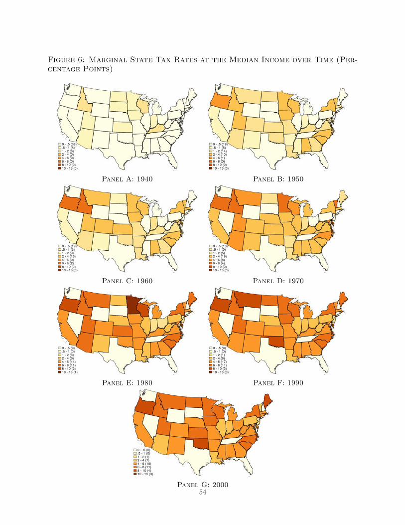
Figure 6: Marginal State Tax Rates at the Median Income over Time (Per-centage Points)

Panel A: 1940 Panel B: 1950

Panel C: 1960 Panel D: 1970

Panel E: 1980 Panel F: 1990

Panel G: 200054

Figure 7: Marginal State Tax Rates at 90th Income Percentile over Time(Percentage Points)

Panel A: 1940 Panel B: 1950

Panel C: 1960 Panel D: 1970

Panel E: 1980 Panel F: 1990

Panel G: 200055

Figure 8: Introduction of State Corporate Taxes

HI WI CT

VA

WV

MO

MT

ND

NM

NY

MA MS

NC

SC TN AR CA

GA

OR

ID

OK

VT

UT AL

AZ

KS

MN

IA LA

PA

SD

KY CO

MD

DC RI AK DE

NJ

IN MI

NE

IL

ME

NH FL

OH

1902

1913

1915

1917

1919

1920

1921

1922

1923

1928

1929

1931

1932

1933

1934

1935

1936

1937

1939

1947

1949

1958

1963

1968

1969

1970

1972

01

23

4N

umbe

r of S

tate

s In

trodu

cing

Cor

pora

te T

axes

Notes: Figure plots the first year in which each state has a statutory corporate income tax rate.

56

Figure 9: Top State Corporate Marginal Tax Rates over Time (PercentagePoints)

Panel A: 1940 Panel B: 1950

Panel C: 1960 Panel D: 1970

Panel E: 1980 Panel F: 1990

Panel G: 200057

Figure 10: Event Studies around Large State Tax Changes

Panel A: Change in Median Panel B: Change in TopPersonal Income Tax Rate Corporate Tax Rate

−.6

−.4

−.2

0.2

Effe

ct o

f Lar

ge T

ax In

crea

seon

Pat

ents

per

10,

000

−4 −3 −2 −1 0 1 2 3 4Years Since Tax Reform

−.6

−.4

−.2

0.2

Effe

ct o

f Lar

ge T

ax In

crea

seon

Pat

ents

per

10,

000

−4 −3 −2 −1 0 1 2 3 4Years Since Tax Reform

−.6

−.4

−.2

0.2

Effe

ct o

f Lar

ge T

ax In

crea

seon

Inve

ntor

s pe

r 10

,000

−4 −3 −2 −1 0 1 2 3 4Years Since Tax Reform

−.8

−.6

−.4

−.2

0.2

Effe

ct o

f Lar

ge T

ax In

crea

seon

Inve

ntor

s pe

r 10

,000

−4 −3 −2 −1 0 1 2 3 4Years Since Tax Reform

Notes: Figure plots the coefficients on event time dummies relative to the reform event time. Year 0 is the first fiscalyear during which the new (higher) tax is applicable. The left panel (A) considers state-level changes in patentingand inventor counts per 10,000 state residents around large changes (all redefined as tax increases) in the personalincome marginal tax rate at the median earnings. The right panel (B) considers changes in innovation around largechanges (relabeled as increases) in the top corporate tax rate. A “large” tax change is defined to be in the top 10%of non-zero year-over-year tax increases (at least 6.85 percentage points for personal income taxes, and 14.8pp forcorporate taxes) or decreases (at least 3.6pp for personal income taxes, and 9.3pp for corporate taxes). Large reformswith a second reform within 4 years, either before or after, are excluded. All regressions include calendar year fixedeffects and reform fixed effects. 95% confidence intervals in gray.

58

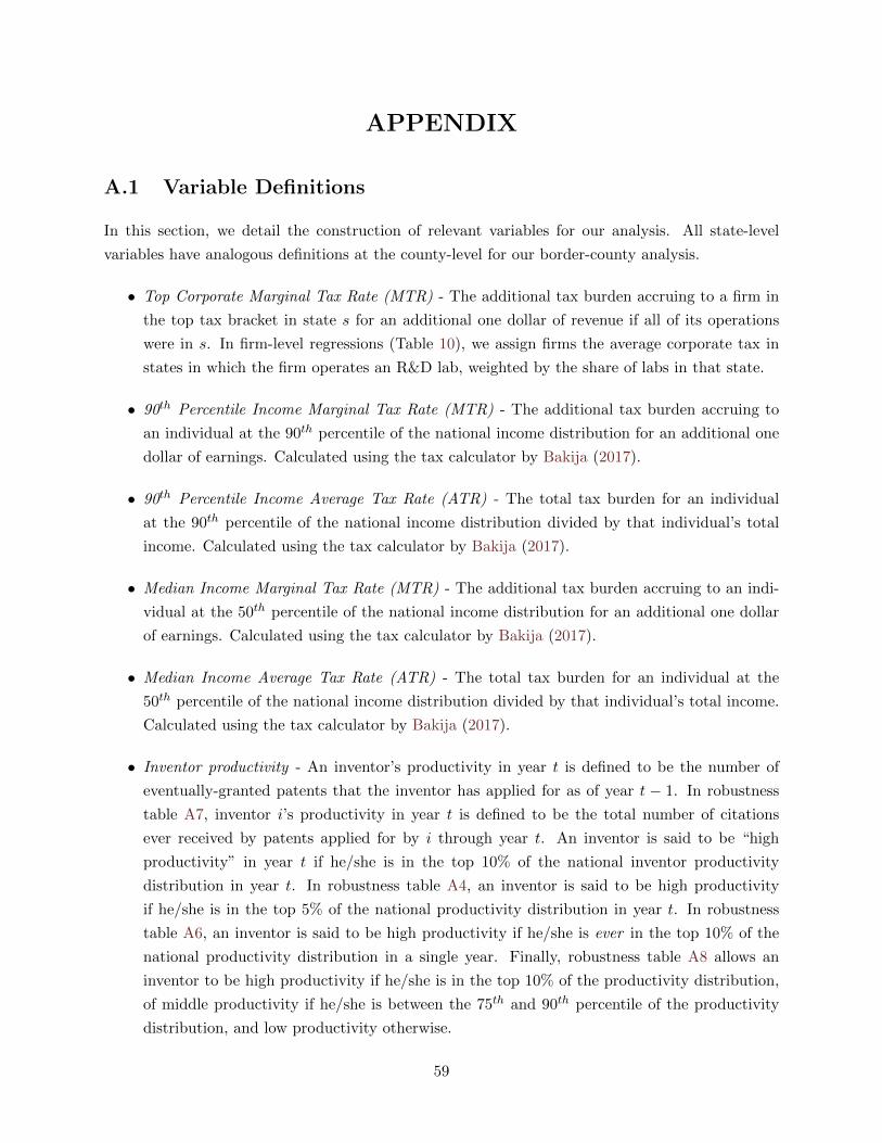
APPENDIX

A.1 Variable Definitions

In this section, we detail the construction of relevant variables for our analysis. All state-level

variables have analogous definitions at the county-level for our border-county analysis.

• Top Corporate Marginal Tax Rate (MTR) - The additional tax burden accruing to a firm in

the top tax bracket in state s for an additional one dollar of revenue if all of its operations

were in s. In firm-level regressions (Table 10), we assign firms the average corporate tax in

states in which the firm operates an R&D lab, weighted by the share of labs in that state.

• 90th Percentile Income Marginal Tax Rate (MTR) - The additional tax burden accruing to

an individual at the 90th percentile of the national income distribution for an additional one

dollar of earnings. Calculated using the tax calculator by Bakija (2017).

• 90th Percentile Income Average Tax Rate (ATR) - The total tax burden for an individual

at the 90th percentile of the national income distribution divided by that individual’s total

income. Calculated using the tax calculator by Bakija (2017).

• Median Income Marginal Tax Rate (MTR) - The additional tax burden accruing to an indi-

vidual at the 50th percentile of the national income distribution for an additional one dollar

of earnings. Calculated using the tax calculator by Bakija (2017).

• Median Income Average Tax Rate (ATR) - The total tax burden for an individual at the

50th percentile of the national income distribution divided by that individual’s total income.

Calculated using the tax calculator by Bakija (2017).

• Inventor productivity - An inventor’s productivity in year t is defined to be the number of

eventually-granted patents that the inventor has applied for as of year t − 1. In robustness

table A7, inventor i’s productivity in year t is defined to be the total number of citations

ever received by patents applied for by i through year t. An inventor is said to be “high

productivity” in year t if he/she is in the top 10% of the national inventor productivity

distribution in year t. In robustness table A4, an inventor is said to be high productivity

if he/she is in the top 5% of the national productivity distribution in year t. In robustness

table A6, an inventor is said to be high productivity if he/she is ever in the top 10% of the

national productivity distribution in a single year. Finally, robustness table A8 allows an

inventor to be high productivity if he/she is in the top 10% of the productivity distribution,

of middle productivity if he/she is between the 75th and 90th percentile of the productivity

distribution, and low productivity otherwise.

59

• Effective Tax Rates - An inventor’s effective marginal (average) tax rate is defined to be

the marginal (average) tax rate faced by the 90th percentile earner in the national income

distribution if the inventor is high productivity, and the marginal (average) tax rate faced by

a median earner if the inventor is low productivity. In appendix table A8, middle productivity

inventors have an effective tax rate equal to the tax rate faced by an individual earning at the

75th percentile of the national income distribution. In all regressions, we use lagged effective

tax rates as independent variables. Thus an inventor living in state s will face an effective tax

rate for innovation output in year t which is the effective tax rate the inventor would have

faced in year t − 1 given his/her t − 1 productivity level and the tax laws in place in year

t− 1.

• Log Patents - The natural logarithm of the number of eventually-granted patents applied for

in state s in year t. Similarly, in firm regressions (Table 10), Log Patents refers to the natural

logarithm of the number of successful patent applications for firm j in year t.

• Log Citations - The natural logarithm of the number of citations ever received by eventually-

granted patents which were applied for in state s in year t. Similarly, in firm regressions (Table

10), Log Citations refers to the natural logarithm of the number of citations ever received

by eventually-granted patents which were applied for by firm j in year t. Citation counts

adjusted according to the algorithm of Hall et al. (2001), detailed for our data in Akcigit

et al. (2017) Appendix B.1.

• Log Inventors - The natural logarithm of number of inventors in state s in year t as implied by

the Lai et al. (2014) algorithm applied to our dataset. A detailed description of this algorithm

is provided in Appendix OA.1.

• Log Superstars - The natural logarithm of the number of inventors in state s in year t who

are in the top 5% of the national inventor productivity distribution.

• Corporate Patent - A corporate patent is one which is assigned to a corporation after being

granted.

• Share Assigned - The share of patents in state s in year t which are assigned to a corporation.

• Log Patents (3-year) - The log of the number of eventually-granted patents applied for by

inventor i in years t through t+ 2.

• Log Citations (3-year) - The log of the number of citations ever received by eventually-granted

patents which were applied for by inventor i in years t through t+2. Citation counts adjusted

according to the algorithm of Hall et al. (2001), detailed for our data in Akcigit et al. (2017)

Appendix B.1.

60

• Has Patent (3-year) - An indicator variable, equal to 100 (for legibility) if the inventor has

at least one successful patent application between years t and t + 2. Inventors are included

in the regression sample for the period between their first ever successful patent application,

and their last ever successful patent application.

• Has 10+ Cites (3-year) - An indicator variable, equal to 100 (for legibility) if the inventor’s

patents, applied for between years t and t+2, ever receive at least 10 citations in total between

them. Inventors are included in the regression sample for the period between their first ever

successful patent application, and their last ever successful patent application. Patent citation

counts adjusted according to the algorithm of Hall et al. (2001), detailed for our data in Akcigit

et al. (2017) Appendix B.1.

• Has Corporate Patent (3-yr) - An indicator variable, equal to 100 (for legibility) if the inventor

successfully applies for at least one patent, which is assigned to a corporation, between years

t and t+ 2. Inventors are included in the regression sample for the period between their first

ever successful patent application, and their last ever successful patent application.

• Corporate Inventor - An inventor is said to be a corporate inventor if he/she is granted at

least one corporate patent in his/her career.

• # of Research Workers - The number of research workers employed by the firm as stated

on the National Research Council (NRC) Surveys of Industrial Research Laboratories of the

United States (IRLUS).

• Agglomeration - The number of patents, in thousands, applied for by inventors j 6= i who

share inventor i’s modal patent class in year t in state s.

• Mover - An inventor is said to be a mover if he/she applies for patents in at least two states

over the sample period. Analagously, non-movers are those inventors who only apply for

patents in one state over the entire course of their career.

• Home State - The state in which an inventor first applies for a patent.

• Assignee Has Patent in Destination - An indicator variable equal to one if an inventor i’s

firm has at least one patent applied for in year t by an inventor j 6= i in destination state s.

• Inventor Tenure/Experience - an inventor’s tenure is the number of years that have passed

since the inventor’s first successful patent application.

61

A.2 Additional Tables and Figures

Table A1: Disambiguation Performance

Sample # Inventors # Patents

1920-2004, All Countries 4,890,574 6,443,2271920-2004, US only 2,734,229 4,208,8761940-2000, US only 1,953,066 2,775,209

Lai et al. Patents, New Disambig. 3,342,989 3,984,771Lai et al. Disambiguation 2,998,661 3,984,771

Lai et al. US Patents, New Disambig. 1,572,011 2,179,741Lai et al. Disambig (US) 1,462,207 2,179,741

Notes: Table shows performance of the Lai et al. disambiguation algorithm as applied to our historical patentdata. Each row contains performance information for a different subsample. The category “Lai et al. Patents, NewDisambig.” reports the performance of our algorithm on the patent records included in the original Lai et al. sample.Likewise, “Lai et al. Disambiguation” reports the number of unique inventors that Lai et al. find when applying theiralgorithm solely to their sample. The first column shows the number of unique inventors found by the disambiguationalgorithm, while the second shows the unique number of patents in each subsample.

62

Table A2: Robustness of Macro Effects of Taxes: State Level Regressions,excluding Federal Taxes or California

Panel A: State Taxes Only

Dependent Variable:Log Log Log Share

Patents Citations Inventors Assigned(1) (2) (3) (4)

Top Corporate MTR (%, lag) -0.053∗∗∗ -0.056∗∗∗ -0.045∗∗∗ -0.799∗∗∗

(0.008) (0.009) (0.007) (0.142)

90th Pctile Income MTR (%, lag) -0.026∗∗∗ -0.021∗∗∗ -0.027∗∗∗ -0.018(0.002) (0.003) (0.002) (0.065)

Median Income MTR (%, lag) -0.042∗∗∗ -0.041∗∗∗ -0.042∗∗∗ -0.085(0.004) (0.004) (0.004) (0.090)

90th Pctile Income ATR (%, lag) -0.047∗∗∗ -0.040∗∗∗ -0.046∗∗∗ -0.011(0.003) (0.004) (0.003) (0.093)

Median Income ATR (%, lag) -0.095∗∗∗ -0.102∗∗∗ -0.086∗∗∗ -0.691∗∗∗

(0.008) (0.010) (0.007) (0.143)

Panel B: Excluding CA, Including Federal Taxes

Top Corporate MTR (%, lag) -0.056∗∗∗ -0.050∗∗∗ -0.045∗∗∗ -1.007∗∗∗

(0.006) (0.007) (0.006) (0.146)

90th Pctile Income MTR (%, lag) -0.055∗∗∗ -0.052∗∗∗ -0.053∗∗∗ -0.390∗∗∗

(0.005) (0.006) (0.005) (0.072)

Median Income MTR (%, lag) -0.076∗∗∗ -0.083∗∗∗ -0.073∗∗∗ -0.337∗∗∗

(0.005) (0.006) (0.005) (0.086)

90th Pctile Income ATR (%, lag) -0.107∗∗∗ -0.111∗∗∗ -0.102∗∗∗ -0.453∗∗∗

(0.006) (0.008) (0.005) (0.105)

Median Income ATR (%, lag) -0.099∗∗∗ -0.105∗∗∗ -0.090∗∗∗ -0.585∗∗∗

(0.007) (0.010) (0.007) (0.144)

Observations 2806 2806 2806 2806Mean of Dep. Var. 6.99 9.64 7.12 71.97S.D. of Dep. Var. 1.24 1.48 1.25 14.32

Notes: Panel A reports estimates in which only state tax rates are included in tax measures. Panel B reportsestimates where federal tax rates are included in the tax measures (as in the baseline table), but we drop Californiafrom our analysis. Row definitions, tax rate variable definitions, estimation period, standard errors, weighting, andcontrols all identical to those specified in the footnote of Table 2. ∗p < 0.1,∗∗ p < 0.05,∗∗∗ p < 0.01.

63

Table A3: Robustness Checks: IV Strategy

Panel A: State-Level Non-Movers (IV)

Dependent Variable:Log Log Log Share

Patents Citations Inventors Assigned(1) (2) (3) (4)

Top Corporate MTR (%, lag) -0.068∗∗∗ -0.068∗∗∗ -0.055∗∗∗ -1.055∗∗∗

(0.008) (0.009) (0.007) (0.182)

90th Pctile Income MTR (%, lag) -0.048∗∗∗ -0.048∗∗∗ -0.046∗∗∗ -0.427∗∗∗

(0.005) (0.007) (0.005) (0.083)

Median Income MTR (%, lag) -0.033∗∗∗ -0.025∗∗∗ -0.034∗∗∗ 0.169∗

(0.003) (0.005) (0.003) (0.087)

90th Pctile Income ATR (%, lag) -0.062∗∗∗ -0.055∗∗∗ -0.060∗∗∗ -0.088(0.006) (0.008) (0.005) (0.118)

Median Income ATR (%, lag) -0.096∗∗∗ -0.102∗∗∗ -0.088∗∗∗ -0.525∗∗∗

(0.011) (0.014) (0.010) (0.176)

Observations 2867 2867 2867 2867Mean of Dep. Var. 6.90 9.56 7.11 68.40S.D. of Dep. Var. 1.30 1.57 1.32 14.66

Panel B: Border County Pairs, Total Effects (IV)

Dependent Variable:Log Log Log Log Corp.

Patents Citations Inventors Patents

Top Corporate MTR (%, lag) -0.065∗∗∗ -0.110∗∗∗ -0.051∗∗∗ -0.066∗∗∗

(0.015) (0.022) (0.019) (0.017)

90th Pctile Income MTR (%, lag) -0.023∗∗∗ -0.025∗∗∗ -0.019∗∗∗ -0.021∗∗∗

(0.005) (0.006) (0.005) (0.006)

Median Income MTR (%, lag) -0.074∗∗∗ -0.080∗∗∗ -0.048∗∗∗ -0.062∗∗∗

(0.007) (0.011) (0.008) (0.008)

90th Pctile Income ATR (%, lag) -0.089∗∗∗ -0.099∗∗∗ -0.063∗∗∗ -0.075∗∗∗

(0.008) (0.010) (0.009) (0.009)

Median Income ATR (%, lag) -0.162∗∗∗ -0.185∗∗∗ -0.134∗∗∗ -0.143∗∗∗

(0.019) (0.025) (0.017) (0.021)

Observations 8289 8289 8289 8217S.D. of Dep. Var. 1.45 1.64 1.49 1.57

Notes: Table reports estimates from instrumental variables regressions similar to those in Panel B of Table 2. PanelA reports state-year level IV regressions in which we only include inventors who never cross state lines. Panel Breports border-county pair regressions similar to those in Panel A of Table 3, except we instrument the difference intax rates with the predicted difference in tax rates given by our Federal tax instrument defined in equations 5 and6. Row definitions, tax rate and instrumental variable definitions, estimation period, standard errors, weighting, andcontrols all identical to those specified in the footnote of Table 2. ∗p < 0.1,∗∗ p < 0.05,∗∗∗ p < 0.01.64

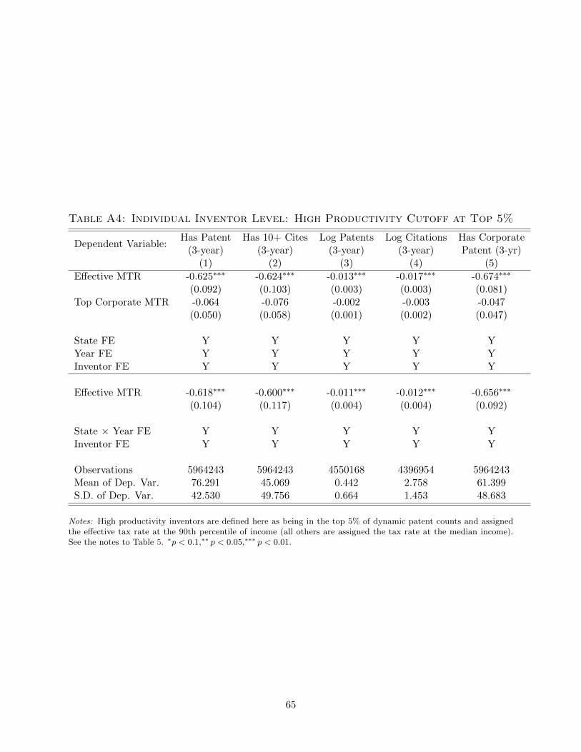
Table A4: Individual Inventor Level: High Productivity Cutoff at Top 5%

Dependent Variable:Has Patent Has 10+ Cites Log Patents Log Citations Has Corporate

(3-year) (3-year) (3-year) (3-year) Patent (3-yr)(1) (2) (3) (4) (5)

Effective MTR -0.625∗∗∗ -0.624∗∗∗ -0.013∗∗∗ -0.017∗∗∗ -0.674∗∗∗

(0.092) (0.103) (0.003) (0.003) (0.081)Top Corporate MTR -0.064 -0.076 -0.002 -0.003 -0.047

(0.050) (0.058) (0.001) (0.002) (0.047)

State FE Y Y Y Y YYear FE Y Y Y Y YInventor FE Y Y Y Y Y

Effective MTR -0.618∗∗∗ -0.600∗∗∗ -0.011∗∗∗ -0.012∗∗∗ -0.656∗∗∗

(0.104) (0.117) (0.004) (0.004) (0.092)

State × Year FE Y Y Y Y YInventor FE Y Y Y Y Y

Observations 5964243 5964243 4550168 4396954 5964243Mean of Dep. Var. 76.291 45.069 0.442 2.758 61.399S.D. of Dep. Var. 42.530 49.756 0.664 1.453 48.683

Notes: High productivity inventors are defined here as being in the top 5% of dynamic patent counts and assignedthe effective tax rate at the 90th percentile of income (all others are assigned the tax rate at the median income).See the notes to Table 5. ∗p < 0.1,∗∗ p < 0.05,∗∗∗ p < 0.01.

65

Table A5: Individual Inventor Level: Only Including States with Progres-sive Tax Spells

Dependent Variable:Has Patent Has 10+ Cites Log Patents Log Citations Has Corporate

(3-year) (3-year) (3-year) (3-year) Patent (3-yr)(1) (2) (3) (4) (5)

Effective MTR -0.390∗∗∗ -0.453∗∗∗ -0.010∗∗∗ -0.014∗∗∗ -0.501∗∗∗

(0.086) (0.100) (0.003) (0.003) (0.068)Top Corporate MTR -0.023 0.064 -0.004 0.001 0.020

(0.117) (0.114) (0.003) (0.004) (0.120)

State FE Y Y Y Y YYear FE Y Y Y Y YInventor FE Y Y Y Y Y

Effective MTR -0.425∗∗∗ -0.449∗∗∗ -0.008∗∗∗ -0.011∗∗∗ -0.509∗∗∗

(0.090) (0.102) (0.003) (0.003) (0.069)

State × Year FE Y Y Y Y YInventor FE Y Y Y Y Y

Observations 2759975 2759975 2095175 2027602 2759975Mean of Dep. Var. 75.913 45.713 0.447 2.814 59.769S.D. of Dep. Var. 42.761 49.816 0.672 1.484 49.036

Notes: See the notes to Table 5. Only state-years undergoing progressive spells included between 1940 and 2000 areincluded here. ∗p < 0.1,∗∗ p < 0.05,∗∗∗ p < 0.01.

66

Table A6: Individual Inventor Level: Using Lifetime Measure of Inventorproductivity

Dependent Variable:Has Patent Has 10+ Cites Log Patents Log Citations Has Corporate

(3-year) (3-year) (3-year) (3-year) Patent (3-yr)(1) (2) (3) (4) (5)

Effective MTR -0.835∗∗∗ -0.532∗∗∗ -0.012∗∗∗ -0.013∗∗∗ -0.559∗∗∗

(0.153) (0.101) (0.003) (0.004) (0.098)Top Corporate MTR -0.131 -0.109 -0.001 -0.001 -0.095

(0.114) (0.102) (0.002) (0.003) (0.096)

State FE Y Y Y Y YYear FE Y Y Y Y YInventor FE Y Y Y Y Y

Effective MTR -0.856∗∗∗ -0.473∗∗∗ -0.010∗∗ -0.010 -0.512∗∗∗

(0.172) (0.127) (0.004) (0.006) (0.116)

State × Year FE Y Y Y Y YInventor FE Y Y Y Y Y

Observations 5960430 5960430 4548136 4394979 5960430Mean of Dep. Var. 76.306 45.078 0.442 2.758 61.407S.D. of Dep. Var. 42.521 49.757 0.664 1.454 48.681

Notes: See the notes to Table 5. High productivity inventors are defined here as ever being in the top 10% of dynamicpatent counts. ∗p < 0.1,∗∗ p < 0.05,∗∗∗ p < 0.01.

67

Table A7: Individual Inventor Level: Using Dynamic Citation Counts

Dependent Variable:Has Patent Has 10+ Cites Log Patents Log Citations Has Corporate

(3-year) (3-year) (3-year) (3-year) Patent (3-yr)(1) (2) (3) (4) (5)

Effective MTR -0.467∗∗∗ -0.458∗∗∗ -0.009∗∗∗ -0.015∗∗∗ -0.515∗∗∗

(0.097) (0.121) (0.003) (0.003) (0.076)Top Corporate MTR -0.243∗∗ -0.144 -0.003∗ -0.001 -0.131

(0.101) (0.100) (0.002) (0.002) (0.091)

State FE Y Y Y Y YYear FE Y Y Y Y YInventor FE Y Y Y Y Y

Effective MTR -0.425∗∗∗ -0.394∗∗∗ -0.007∗∗ -0.012∗∗∗ -0.456∗∗∗

(0.101) (0.131) (0.003) (0.003) (0.079)

State × Year FE Y Y Y Y YInventor FE Y Y Y Y Y

Observations 5960430 5960430 4548136 4394979 5960430Mean of Dep. Var. 76.306 45.078 0.442 2.758 61.407S.D. of Dep. Var. 42.521 49.757 0.664 1.454 48.681

Notes: See the notes to Table 5. High productivity inventors defined here as being in the top 10% of the dynamiccitation counts. ∗p < 0.1,∗∗ p < 0.05,∗∗∗ p < 0.01.

68

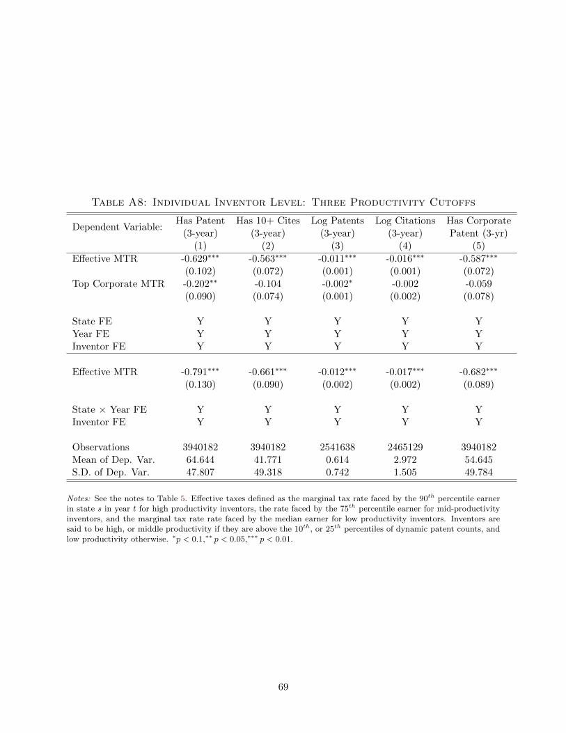
Table A8: Individual Inventor Level: Three Productivity Cutoffs

Dependent Variable:Has Patent Has 10+ Cites Log Patents Log Citations Has Corporate

(3-year) (3-year) (3-year) (3-year) Patent (3-yr)(1) (2) (3) (4) (5)

Effective MTR -0.629∗∗∗ -0.563∗∗∗ -0.011∗∗∗ -0.016∗∗∗ -0.587∗∗∗

(0.102) (0.072) (0.001) (0.001) (0.072)Top Corporate MTR -0.202∗∗ -0.104 -0.002∗ -0.002 -0.059

(0.090) (0.074) (0.001) (0.002) (0.078)

State FE Y Y Y Y YYear FE Y Y Y Y YInventor FE Y Y Y Y Y

Effective MTR -0.791∗∗∗ -0.661∗∗∗ -0.012∗∗∗ -0.017∗∗∗ -0.682∗∗∗

(0.130) (0.090) (0.002) (0.002) (0.089)

State × Year FE Y Y Y Y YInventor FE Y Y Y Y Y

Observations 3940182 3940182 2541638 2465129 3940182Mean of Dep. Var. 64.644 41.771 0.614 2.972 54.645S.D. of Dep. Var. 47.807 49.318 0.742 1.505 49.784

Notes: See the notes to Table 5. Effective taxes defined as the marginal tax rate faced by the 90th percentile earnerin state s in year t for high productivity inventors, the rate faced by the 75th percentile earner for mid-productivityinventors, and the marginal tax rate rate faced by the median earner for low productivity inventors. Inventors aresaid to be high, or middle productivity if they are above the 10th, or 25th percentiles of dynamic patent counts, andlow productivity otherwise. ∗p < 0.1,∗∗ p < 0.05,∗∗∗ p < 0.01.

69

Figure A1: Inventors per 10,000 State Residents Over Time

Panel A: 1940 Panel B: 1950

Panel C: 1960 Panel D: 1970

Panel E: 1980 Panel F: 1990

Panel G: 2000

70

Figure A2: Trends in R&D Lab Operations

020

0040

0060

00#

Res

earc

h La

bs

1920 1930 1940 1950 1960 1970Year

Panel A: Total Number of Labs

5000

1000

015

000

2000

025

000

# P

aten

ts fr

om R

esea

rch

Labs

1920 1930 1940 1950 1960 1970Year

5000

1000

015

000

2000

025

000

# C

itatio

ns fr

om P

aten

ts o

f Res

earc

h La

bs

1920 1930 1940 1950 1960 1970Year

Panel B: Total Patents from Labs Panel C: Citations Received by Labs

010

0000

2000

0030

0000

4000

0050

0000

# R

esea

rch

Wor

kers

1920 1930 1940 1950 1960 1970Year

2040

6080

100

Res

earc

h W

orke

rs p

er R

esea

rch

Lab

1920 1930 1940 1950 1960 1970Year

Panel D: Total Research Workers Panel E: Mean Research Workers per Lab

Notes: Figure plots trends in R&D labs from the National Research Council Surveys of Industrial Research Labora-tories of the United States (IRLUS).

71

Figure A3: Firm Patent Distributions

010

2030

40Pe

rcen

t of f

irms

with

at l

east

one

pat

ent

19211927

19311933

19381940

19461950

19561960

19651970

Panel A: % of Firms with Patents

010

2030

40Pe

rcen

t

0 10 20 30 40 50+Number of Patents Granted To Firm in Year

Pr{Patents > 0} = 21.58, Cond. Median = 3, Cond. Mean = 10.28

Panel B: Patents per Firm per Year 1920-1970

1025

5010

020

0N

umbe

r of P

aten

ts(L

og S

cale

, Pro

duct

ive

Firm

s)

24

68

10N

umbe

r of P

aten

ts

1920 1930 1940 1950 1960 1970Year

Median 75th 90th (RHS)95th (RHS) 99th (RHS)

Panel C: Patents per firm over time

Notes: Figure plots distributions of patenting amongst firms with an R&D labs in the National Research CouncilSurveys of Industrial Research Laboratories of the United States (IRLUS). The top panel plots the share of firms ineach survey year which have at least one patent in that year. Panel B plots the distribution of firm patenting peryear over the R&D lab sample of 1920-1970, conditional on the firm having at least one patent. Panel C plots thetime series of the firm-year level patenting distribution, conditional on having at least one patent.

72

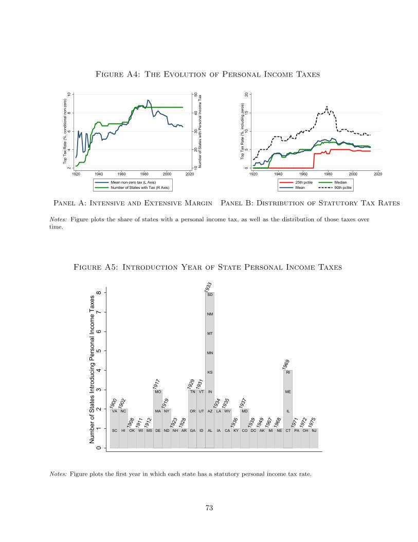
Figure A4: The Evolution of Personal Income Taxes

1020

3040

50N

umbe

r of S

tate

s w

ith P

erso

nal I

ncom

e Ta

x

24

68

10To

p Ta

x R

ate

(%, c

ondi

tiona

l non

-zer

o)

1920 1940 1960 1980 2000 2020

Mean non-zero tax (L Axis)Number of States with Tax (R Axis)

05

1015

20To

p Ta

x R

ate

(%, i

nclu

ding

zer

os)

1920 1940 1960 1980 2000 2020

25th pctile MedianMean 90th pctile

Panel A: Intensive and Extensive Margin Panel B: Distribution of Statutory Tax Rates

Notes: Figure plots the share of states with a personal income tax, as well as the distribution of those taxes overtime.

Figure A5: Introduction Year of State Personal Income Taxes

SC

VA

HI

NC

OK WI MS DE

MA

MO

ND

NY

NH AR GA

OR

TN

ID

UT

VT

AL

AZ

IN

KS

MN

MT

NM

SD

IA

LA

CA

WV

KY CO

MD

DC AK MI NE CT

IL

ME

RI

PA OH NJ

1900

1902

1908

1911

1912

1917

1919

1923

1928

1929

1931

1933

1934

1935

1936

1937

1939

1949

1967

1968

1969

1971

1972

1975

01

23

45

67

8N

umbe

r of S

tate

s In

trodu

cing

Per

sona

l Inc

ome

Taxe

s

Notes: Figure plots the first year in which each state has a statutory personal income tax rate.

73

Figure A6: The Evolution of Personal Income Taxes in Select States

05

1015

Stat

e To

p M

argi

nal T

ax R

ate

1920 1930 1940 1950 1960 1970 1980 1990 2000 2010Year

CA IL NJNY PA

02

46

810

Stat

e M

argi

nal T

ax R

ate

for 5

0th

Perc

entil

e

1920 1930 1940 1950 1960 1970 1980 1990 2000 2010Year

CA IL NJNY PA

Panel A: Time Series of Key States’ Panel B: Time Series of Key States’Top Statutory MTR MTR for Median Earner

Notes: Figure plots the time series of marginal personal income tax rates for the five most innovative states in oursample.

74

Figure A7: The Evolution of Corporate Taxes

1020

3040

50N

umbe

r of S

tate

s w

ith C

orpo

rate

Tax

34

56

78

Top

Tax

Rat

e (%

, con

ditio

nal n

on-z

ero)

1920 1940 1960 1980 2000 2020

Mean non-zero tax (L Axis)Number of States with Tax (R Axis)

Panel A: Intensive and Extensive Margin

02

46

810

Top

Tax

Rat

e (%

, inc

ludi

ng z

eros

)

1920 1940 1960 1980 2000 2020

10th pctile MedianMean 90th pctile

Panel B: Distribution of Statutory Tax Rates

05

1015

Top

Cor

pora

te M

argi

nal T

ax R

ate

(%)

1920 1930 1940 1950 1960 1970 1980 1990 2000 2010Year

CA IL NJNY PA

Panel C: Time Series of Select States

Notes: Figure plots the time series of the distribution and proliferation of state corporate tax rates. Panel A showsthe number of states with a corporate income tax and the mean non-zero tax rate. Panel B plots the distributionof top state corporate tax rates over time. Panel C shows the evolution of top state corporate tax rates for the fivemost innovative states in our sample.

75

Figure A8: Binned Scatter Plots: State Regressions-.4

-.20

.2.4

Res

idua

lized

Log

Pat

ents

-4 -2 0 2 4Residualized Median Earner Personal Income MTR (%)

-.3-.2

-.10

.1.2

Res

idua

lized

Log

Pat

ents

-4 -2 0 2 4Residualized 90th Percentile Earner Personal Income MTR (%)

-.2-.1

0.1

.2R

esid

ualiz

ed L

og P

aten

ts

-2 -1 0 1 2Residualized Top Corporate MTR (%)

-.6-.4

-.20

.2R

esid

ualiz

ed L

og C

itatio

ns R

ecei

ved

(194

7 on

)

-4 -2 0 2 4Residualized Median Earner Personal Income MTR (%)

-.3-.2

-.10

.1.2

Res

idua

lized

Log

Cita

tions

Rec

eive

d (1

947

on)

-4 -2 0 2 4Residualized 90th Percentile Earner Personal Income MTR (%)

-.2-.1

0.1

.2R

esid

ualiz

ed L

og C

itatio

ns R

ecei

ved

(194

7 on

)

-2 -1 0 1 2Residualized Top Corporate MTR (%)

-.4-.2

0.2

.4R

esid

ualiz

ed L

og In

vent

ors

-4 -2 0 2 4Residualized Median Earner Personal Income MTR (%)

-.3-.2

-.10

.1R

esid

ualiz

ed L

og In

vent

ors

-4 -2 0 2 4Residualized 90th Percentile Earner Personal Income MTR (%)

-.2-.1

0.1

.2R

esid

ualiz

ed L

og In

vent

ors

-2 -1 0 1 2Residualized Top Corporate MTR (%)

Notes: Figure plots binned scatter plots of effect of taxes at state level. The top row shows the effect on log patents, the middle row present scatters for logcitations, while the bottom row shows log inventors. The leftmost column shows the effect of median income marginal tax rates, the middle column shows theeffect of MTRs for the 90th percentile earners, and the rightmost column show effect of top corporate MTRs. All tax rates include both federal and state taxes.Both the horizontal and vertical axes are residualized against state and year fixed effects, as well as lagged population density, GDP per capita, and R&D taxcredits.

76

A.3 Case Studies

We present here three special episodes of tax reform in New York, Delaware, and Michigan to

provide some sharp visual evidence of the effects of taxes on innovation. Figures A9-A10 show the

results from each of these episodes. In each case, the black solid line represents the time series in

the state under consideration, while the dashed line represents a control state. The control state

is constructed according to the synthetic control method of Abadie et al. (2010). That is, it is a

weighted average of other states in the sample, where the weights are chosen to best match the

average innovation outcome of interest (patents, inventors, or citations), as well as real GDP per

capita and population density for the period before the tax change in the state of interest.

For the case of New York, the control state turns out to be California. For Michigan and

Delaware, it is a combination of other states. For the post-tax change period, the synthetic state

represents a plausible counterfactual of what may have happened in the state of interest absent the

tax change. The first panel shows log patents, the second shows log inventors and the third shows

log citations. The dashed vertical lines (or, for Michigan the gray area) represents the timing of

the tax change.

New York 1968 vs. California

The first case study is shown in Figure A9 and concerns New York’s 1968 tax reform bill, in which

the top marginal personal income tax rate increased from 10% to 14% and its state top corporate

tax rate increased from 5.5% to 7%. The control state here is California, where the top tax rate

increased as well from 7% to 10%, but remained lower while the corporate tax rate remained the

same at 5.5%. All variables are normalized at their 1965 levels. Before the tax bill, New York and

California follow remarkably similar trends for all three innovation outcomes. However, after the

reform, they diverge and New York performs much worse in terms of innovation relative to the

synthetic control.

Michigan 1967-1968

Figure A10 shows the case study of Michigan. Michigan introduced its personal state tax rate in

1967 at 2.6%. One year later, in 1968, it introduced its corporate state tax at 5.6%. The synthetic

control for Michigan is composed of several variations on California, Ohio/Pennsylvania, and, for

some of the outcome variables, a bit of Texas. While the control state and Michigan evolve very

similarly before 1967, Michigan starts performing significantly worse for the innovation outcome

measures after the introduction of its tax regime.

Delaware 1969-1970

The third case study concerns Delaware. In July 1969, the corporate tax rate increased from 5%

to 6%, and in August 1971 a temporary surcharge of 20% was added on top of the 6% corporate

77

tax rate. In 1970, the personal tax rate increased from 11% to 18%. In this case, the best-fitting

synthetic control is comprised of Nevada, California, and Connecticut. Figure A11 shows that the

effects on patents, citations, and inventors were noticeably large with the negative trend setting in

at the time of the tax reform.

These case studies provide particularly clear visual evidence of a strong negative relationship

between taxes and innovation. When combined with the macro state-level regressions, the instru-

mental variable approach and the border county analysis, the results overall bolster the conclusion

that taxes were significantly negatively related to innovation outcomes at the state level.

78

Figure A9: Synthetic Control Analysis: New York 1968

.6.7

.8.9

1Lo

g Pa

tent

s R

elat

ive

to 1

965

1960 1965 1970 1975 1980Year

Innovation: NY Innovation: Synthetic NYTop 3 synthetic control states: CA (1.000), OK (0.000), ND (0.000)

.7.8

.91

Log

Inve

ntor

s R

elat

ive

to 1

965

1960 1965 1970 1975 1980Year

Innovation: NY Innovation: Synthetic NYTop 3 synthetic control states: CA (1.000), TX (0.000), UT (0.000)

.6.8

11.

21.

41.

6Lo

g C

itatio

ns R

elat

ive

to 1

965

1960 1965 1970 1975 1980Year

Innovation: NY Innovation: Synthetic NYTop 3 synthetic control states: CA (1.000), ME (0.000), OK (0.000)

Notes: Figure plots synthetic control analyses for New York’s 1968 tax reform bill, in which the top marginal personalincome tax rate increased from 10% to 14%, and its state corporate tax rate increased from 5.5% to 7%. The firstrow shows the patterns for log patents, the middle row for log inventors, and the bottom row for log citations. Wenormalize the patent counts for synthetic and actual New York to be the same in 1965.

79

Figure A10: Synthetic Control Analysis: Michigan 1967-68

7.4

7.6

7.8

88.

2Lo

g Pa

tent

s

1950 1960 1970 1980 1990Year

Innovation: MI Innovation: Synthetic MITop 3 synthetic control states: CA (0.514), PA (0.239), TX (0.116)

7.2

7.4

7.6

7.8

88.

2Lo

g In

vent

ors

1950 1960 1970 1980 1990Year

Innovation: MI Innovation: Synthetic MITop 3 synthetic control states: CA (0.503), PA (0.185), TX (0.103)

9.5

1010

.511

Log

Cita

tions

1950 1960 1970 1980 1990Year

Innovation: MI Innovation: Synthetic MITop 3 synthetic control states: CA (0.468), OH (0.219), TX (0.077)

Notes: Figure plots synthetic control analyses Michigan around its major reforms in 1967 and 1968. In 1967, Michiganintroduced its personal income tax, at a rate of 2.6%. In 1968, it then introduced its corporate income tax, at a rateof 5.6%. The first row shows the patterns for log patents, the middle row for log inventors, and the bottom row forlog citations.

80

Figure A11: Synthetic Control Analysis: Delaware 1969-71

5.6

5.8

66.

26.

46.

6Lo

g Pa

tent

s

1950 1960 1970 1980 1990Year

Innovation: DE Innovation: Synthetic DETop 3 synthetic control states: CT (0.375), NV (0.371), CA (0.232)

5.6

5.8

66.

26.

46.

6Lo

g In

vent

ors

1950 1960 1970 1980 1990Year

Innovation: DE Innovation: Synthetic DETop 3 synthetic control states: NV (0.396), CT (0.378), CA (0.200)

88.

59

9.5

Log

Cita

tions

1950 1960 1970 1980 1990Year

Innovation: DE Innovation: Synthetic DETop 3 synthetic control states: CT (0.362), NV (0.354), CA (0.254)

Notes: Figure plots synthetic control analyses around Delaware’s tax reforms. In July 1969, the corporate tax rateincreased from 5% to 6%, and in August 1971 a temporary surcharge of 20% was added on top of the 6% corporatetax rate. In 1970, the personal tax rate increased from 11% to 18%. The first row shows the patterns for log patents,the middle row for log inventors, and the bottom row for log citations.

81

ONLINE APPENDIX – NOT FOR PUBLICATION

for “The Effects of Taxes on Innovation: Evidence from Historical

U.S. Patent Data”

by Ufuk Akcigit, John Grigsby, Tom Nicholas, and Stefanie Stantcheva

OA.1 Disambiguation Algorithm

We employ the algorithm of Lai et al. (2014) to disambiguate inventors in our historical patent

data.34 The goal of disambiguation is to determine if two patent-inventor level records were pro-

duced by the same inventor. A problem of this sort may be distilled into a clustering problem

well-suited to standard machine learning algorithms: given a training dataset and a set of features

– such as inventor name, location, technology class, assignee, and coauthor networks – we wish

to group records together into profiles which indicate that the two records were produced by the

same inventor. The goal is to assign probabilities of an inventor match based on the characteristics

of every pair of observations. The central idea is that two records coming from two very similar

names (not necessarily identical: “John A Smith” vs “John Adam Smith” for instance) working in

similar subject areas, working for the same company in roughly the same geographic location, are

likely to be the same person.

Such a machine learning approach has three central benefits relative to other more rudimen-

tary approaches, such as treating each individual name as a separate inventor, or hand-matching

innovators’ records to one another. First, the Lai et al. approach permits minor name typos or

data entry errors, without incorrectly decoupling these inventors. Second, it provides probabilistic

matches based on more information than name and location, which helps disambiguate between

common names – a John Smith working in software is likely different to a John Smith with patents

in bootmaking. Finally, the algorithm does not impose any functional forms on the relationship

between a pair’s set of attributes and the probability that those pairs belong to the same inventor.

Of course, this machine learning approach is imperfect and will struggle to correctly match

inventors who drastically change their names or have exceptional careers. For instance, if an

inventor named Jane Smith changes her name after marrying a man with surname Robertson, the

algorithm will struggle to adapt, as names are the most distinguishing piece of information amongst

records. Similarly, if a software engineer living in California and working for Apple decides to change

his career and move to Montana to open a new shoe factory, the algorithm is likely to suggest that

these are two separate inventors, rather than one inventor with such an uncommon career trajectory.

The clustering exercise is subject to two principal challenges. First, one must produce a suitable

34The code and associated files for the original disambiguation may be downloaded from https://github.com/

funginstitute/downloads; accessed October 13, 2016.

82

training dataset from which to glean the probability that two patent records with a similarity profile

of x belong to the same inventor. Here, one may follow two approaches. One could submit a hand-

curated dataset of known matches to the disambiguation algorithm to determine the likelihood of

a match. However, the construction of these datasets are often subject to bias if, for example,

researchers are more likely to include better-known inventors. An alternative approach, and the

one followed by Lai et al., is to allow the algorithm to produce its own training dataset based on

features in the data. For example, a training dataset of known matches could be constructed by

examining individuals with matching rare names.

Our baseline approach lies somewhere in between these two strategies. We use the matches

of Lai et al. to form the basis of our training dataset. We draw twenty million pairs of records

belonging to different inventors according to Lai et al. to complete our training dataset. Using

this as a training dataset relies on two principal assumptions: first, we assume that the Lai et al.

disambiguation correctly identifies inventors, and second we assume that the sets of features that

were predictive of inventor clustering are stable over time, so that the same rules for determining

matches in the modern sample of Lai et al. will apply to our historical sample. We choose this

approach in order to best match the state-of-the-art disambiguation of inventors in the modern

data.35

The second major challenge to the disambiguation exercise is computational. Ideally, one would

compare every pair of records in our data, and build a similarity profile for each. However, with over

12 million unique patent-inventor records in our dataset, one would have to compare over 144 trillion

record pairs in order to compare each record to each other, which is computationally infeasible. To

circumvent this challenge, we follow Lai et al. in disambiguating successively larger blocks. We

first group records into blocks of possible matches, based on the first characters of an inventor’s

name. Then we compare all records within a block to one another, but never compare across

blocks. After disambiguating a set of narrow blocks, we expand the size of the block, for example

by considering all record pairs that match the first three letters of an inventor’s name, rather than

the first five letters. By iteratively allowing progressively larger blocks, and assuming clusters

within prior blocking rounds were successfully disambiguated, we greatly reduce the computational

burden of the disambiguation.

Our starting point is the historical inventor data digitized by Akcigit et al. (2017), combined

with the patent data of Lai et al. (2014) available on the Harvard Dataverse Network (HDN).36 We

first manually clean inventor names and location to correct for obvious typos. The most common

correction is to remove prefixes and suffixes, such as “DR,” “JR,” and “SR.” In addition, we

standardize names to be all capital letters, and consider a person’s first name to be the first word

of their name. Finally, we consider only the first patent class listed on a patent document to be

35In early versions of the paper, we experimented with allowing the algorithm to find its own training sets, andfound qualitatively similar headline results.

36Accessed from https://dataverse.harvard.edu/dataset.xhtml?persistentId=hdl:1902.1/15705 on Febru-ary 13, 2017.

83

that patent’s primary classification.

To compare records, we construct a similarity profile for every pair of records to be compared.

A similarity profile x is a vector of similarity scores for the active attributes in the disambiguation.

Specifically, a similarity profile is encoded as follows:

• First and Last names

1. If one of the two records is missing the name

2. If there is no clear misspelling or abbreviation employed, and the strings do not exactly

match

3. If there is a misspelling (defined as either missing 1 or 2 characters somewhere, or

switching the place of a few characters)

4. If exact match or, in the case of first names, if one string appears to be an abbreviation

of the other in that it has the first 3 characters the same (e.g. “ROB” and “ROBERT”)

• Middle Names

0. If have different middle names

1. If one of the two records have missing middle name

2. If both records have missing middle name

3. If one record has a full middle name (e.g. “WILLIAM”) and the other has just the

middle initial which matches the full middle name (e.g. “W”).

4. If exactly the same name

• Location

1. If over 50 miles apart

2. If under 50 miles apart

3. If under 25 miles apart

4. If under 10 miles apart

5. If under 1 mile apart

• Patent Classes

0. If different strings

1. If exactly the same string

• Assignees

5. If the Jaro-Winkler string distance between assignee names is at least 0.9

84

4. If JW distance > 0.8

3. If JW distance > 0.7

2. If one of the two records has a missing assignee

1. Otherwise

• Coauthors

1. If coauthors exactly the same (coauthors entered as <First Initial> . <Last Name> and

separated by comma in the variable)

0. Otherwise

• Country

0. If different country

1. If the same non-US country

2. If the same US country

Next, one may construct, for every observed similarity profile, the probability that this profile

belongs to the same inventor or not, by comparing the frequency with which it occurs in the training

dataset. Specifically, defining M to be the set of matched inventor pairs in the training dataset,

and N to be the set of non-matched inventor pairs in the training dataset, one may use Bayes’ rule

to write the probability of a match as

P (M|x) =P (x|M)P (M)

P (x|M)P (M) + P (x|N ) (1− P (M))

where P (M) is the prior probability of a match, which we follow Lai et al. in setting as proportional

to the ratio of the number of within-cluster pairs (i.e. disambiguated inventors from prior blocking

rounds) in a block to the total number of pairs in that block.37 For numerical reasons, it is more

convenient to work with the posterior odds of a match, defined as

P (M|x)

1− P (M|x)=P (x|M)

P (x|N )·

P (M)

1− P (M)

In particular, we calculate the likelihood ratio, r(x), for every observed similarity profile x. This

likelihood ratio is defined as

r(x) =P (x|M)

P (x|N )(OA1)

This can be determined directly from the training dataset by comparing the number of records

with similarity profile x that belong in the matched training dataset (i.e. come from the same

37The discrete nature of the similarity profile space described above makes the computation of this match probabilitymuch simpler.

85

inventor), to the number of records with similarity profile x that belong in the unmatched training

dataset (i.e. come from different inventors).38 Once we have the likelihood ratios calculated, we

invert them to calculate the probability that two records originated from the same inventor:

P (M|x) =1

1 + 1−P (M)P (M)

1r(x)

(OA2)

We say that two records originated from the same inventor if this posterior probability of a match

is at least 0.99.39

Our blocking routine proceeds as follows:40

Round 1. Block based on exact first and last name. Compare records based on middle name and patent

location.

Round 2. Block based on exact first and last name. Compare records based on middle name, coauthor

network, patent class, and assignee name.

Round 3. Block based on first five characters of first name, and exact last name. Compare records

based on middle name, coauthor network, patent class, and assignee name.

Round 4. Block based on first three characters of first name, and exact last name. Compare records

based on middle name, coauthor network, patent class, and assignee name.

Finally, we subset our data to only consider US inventors. As was indeed the case in our time

period, the most productive inventors are Kia Silverbrook, Shunpei Yamazaki, George Lyon, Donald

Weder, and Melvin De Groote. We refer the reader to Lai et al. (2014) for additional statistics on

the performance of the algorithm on modern data.

OA.2 Assigning Inventors to States

Our patent data provides information on the residence address of the patent’s inventors. However,

we do not observe the residence of all inventors on a patent in the historical period. Specifically,

we observe an inventor’s state if either 1) they are the first inventor on the patent, or 2) the patent

is contained in the Harvard Dataverse Network (HDN) data. In order to run our inventor-level

38To account for small sample bias in rare similarity profiles, we follow Lai et al. in applying a Laplace correctionto these likelihood ratio values.

39In the early stages of our analysis, we experimented with match thresholds of 0.98 and 0.95 to determine whetherrecords originated from the same inventor. After examining the data by hand, we determined that this was too low,as common names such as Robert Smith were often spuriously considered the most prolific inventors in the data.This problem largely vanished with the threshold of 0.99.

40We experimented with additional rounds of blocking, as well as with allowing for inexact surname matches in theblocking routine. Manual checks of the data revealed that this routine minimized errors with common names, andcorrectly matched the most productive inventors as listed by outside data sources.

86

regressions, we must assign each inventor to a particular home state. In this section, we detail our

approach to doing so.

For all non-primary authors on historical patents, we impute a location using the following

algorithm:

1. We assign all HDN and first author inventors to the state listed in the data

2. If an inventor is an HDN or first author inventor on one patent in a given year, but not

on another patent, we assign that inventor to his first-author state. If he is first author in

multiple states in that year, we assign him to the state listed on the patent if that state

matches one of his first author states; otherwise we proceed to step 3 below (using alternative

years)

3. We replace the inventor’s state with the preceding years state if state information is still

missing.

4. We replace the inventor’s state with the following years state if state information is still

missing.

5. If the inventor-patent record is still missing state information, but the inventor has multiple

first-author states listed in that year, then we pick a random first-author state for that

inventor-patent.

6. If all else fails, we assign the state of the first-author on the patent.

An additional challenge arises from the fact that a number of inventors have patents granted

in multiple states in the same year. There may be many causes for multiple unique states within

a given year for an inventor. The most common causes of these multi-state inventors are:

• An inventor may live in state A until midway through a particular year, and then move to

state B. They file a patent application both in state A before moving and in state B after

moving. They never file a patent in state B before moving, and never file a patent in state A

after moving.

• Inventors may have multiple home addresses. As a result, they consistently file in both state A

and state B in multiple years. For example, inventors may spend half of the year in Chicago,

IL, and half of the year in Milwaukee, WI, and thus frequently have patents in both of these

states in a given year.

• Inventors have multiple coauthors, who live in different states and who alternate in terms of

who is the first listed author. For instance, Harvey Clayton Rentschler lives in Pittsburgh, PA,

but frequently coauthors with J. Marden, who lives in Orange, NJ. Every time they coauthor

a patent, the location is listed as Orange, NJ, but every time Harvey Rentschler sole authors

a patent, his location appears to be Pittsburgh. These situations are particularly common

87

among assigned patents, and seem to account for all individuals living in an exceptionally

high number of states. Indeed, everyone who shows up in 7 or more states has a coauthor

on their patents, while the share of those with a coauthor is 92.8% for those with multiple

states, compared with just 66.3% for those in one state41

• Possible disambiguation errors: two individuals may have very similar names, work in similar

classes, and live just across a state border from one another (so are close in latitude-longitude).

As a result these two separate inventors may be classified as the same person by the disam-

biguator. This would inflate the number of states an individual lives in.

To address this concern, we assign multi-state inventors a home state using the following algo-

rithm:

1. Each year, assign an inventor to the modal state in which we observe him/her operating as a

sole author.

2. If the inventor does not have any sole authorships in that particular year, check if he/she has

sole authorships in the preceding or subsequent year. If the preceding and subsequent year

both have sole authorships in the same modal location, then assign the inventor to that state.

This smoothes over off years for inventors and removes spurious migration.

3. If we still do not have a location for the inventor, then we assign them to the modal location

we observe them in in the given year, regardless of whether the patent was sole authored or

coauthored.

4. If the inventor has two modal states (e.g. has 2 patents in both Illinois and Wisconsin in the

given year), then choose a random choice of those states and assign the inventor to that state.

OA.3 Historical Corporate Tax Data

We collected the corporate tax rates from a large variety of sources. We have built a documen-

tation available at https://scholar.harvard.edu/stantcheva/publications that shows all the

sources for each year and state. We only collected direct taxes and net income franchise taxes. We

also collect surtaxes or surcharges, as well as additional temporary taxes imposed on top of the

main rates. They are sometimes imposed as a percentage of regular tax liabilities and sometimes

as a rate to add to the main rate. We record them as rates to add to the main rate with applicable

thresholds. We have not collected minimum taxes (they are very low and probably not applicable

to the companies in our sample) and alternative minimum taxes.

41This is partially mechanical as these inventors are also more productive so have more chances to appear inmultiple states.

88