STEM: An approach to Multi-source Domain Adaptation with Guarantees

Van-Anh Nguyen1, Tuan Nguyen2, Trung Le2, Quan Hung Tran3, Dinh Phung2,4

1VNU - University of Science, Vietnam2Department of Data Science and AI, Monash University, Australia

3Adobe Research, San Jose, CA, USA4VinAI Research, Vietnam

vananhnt57@gmail.com, {tuan.ng, trunglm}@monash.edu,

qtran@adobe.com, dinh.phung@monash.edu

Abstract

Multi-source Domain Adaptation (MSDA) is more prac-tical but challenging than the conventional unsuperviseddomain adaptation due to the involvement of diverse mul-tiple data sources. Two fundamental challenges of MSDAare: (i) how to deal with the diversity in the multiple sourcedomains and (ii) how to cope with the data shift betweenthe target domain and the source domains. In this paper,to address the first challenge, we propose a theoretical-guaranteed approach to combine domain experts locallytrained on its own source domain to achieve a combinedmulti-source teacher that globally predicts well on the mix-ture of source domains. To address the second challenge,we propose to bridge the gap between the target domainand the mixture of source domains in the latent space via agenerator or feature extractor. Together with bridging thegap in the latent space, we train a student to mimic the pre-dictions of the teacher expert on both source and target ex-amples. In addition, our approach is guaranteed with rigor-ous theory offered insightful justifications of how each com-ponent influences the transferring performance. Extensiveexperiments conducted on three benchmark datasets showthat our proposed method achieves state-of-the-art perfor-mances to the best of our knowledge.

1. Introduction

Recent advances in deep learning have enjoyed greatsuccess in performing visual learning tasks under the col-lection of massive annotated data [26, 64, 50, 54, 3]. How-ever, directly transferring knowledge of a learned model,which is trained on a source domain, to a novel targetdomain can undesirably degrade its performance due tothe existence of domain and label shifts [49]. To ad-dress these issues, a diverse range of approaches in do-

main adaptation (DA) has been proposed from shallow do-main adaptation [45, 16, 5, 6] to deep domain adaptation[13, 32, 51, 12, 55, 9, 29, 41, 40]. While the conventionalDA aims to transfer knowledge from a labeled source do-main to an unlabeled target domain, in many real-worldcontexts, labeled data are collected from multiple domains,for example, images taken under different conditions (e.g.,weather, poses, lighting conditions, distinct backgrounds,and etc) [70]. This has arisen a very practical and use-ful setting for transfer learning named multi-source domainadaptation (MSDA) in which we need to transfer knowledgefrom multiple distinct source domains to a single unlabeledtarget domain.

For multi-source domain adaptation, there exist two fun-damental challenges: (i) how to deal with the diversity inthe labeled source domains and (ii) how to cope with thedomain shift between the target domain and the source do-mains. The first challenge makes it harder to train a singlemodel that is expected to work well on multiple source do-mains due to the requirement to resolve diverge data com-plexity imposed on model training. To overcome this chal-lenge, inspired by [36, 23], we propose combining domainexperts into a multi-source teacher by mixing the domainexpert predictions using the coefficients learned by a do-main discriminator. Our rigorous theory demonstrates thatthe performance of this multi-source teacher expert predict-ing globally on the mixture source domains is at least bet-ter than that of the worst domain expert predicting locallyon its domain (see Theorem 1). Therefore, if we can trainqualified domain experts, their combination leads to anotherqualified expert with significantly broader coverage.

To address the second challenge, as suggested by The-orem 3, we employ a joint feature extractor that maps thetarget domain and the mixture of source domains into thesame latent space with the help of adversarial learning. Fur-thermore, together with closing the divergence of the targetdomain and mixture of source domains on the latent space,

9352

we train a target-domain student to imitate the multi-sourceteacher on both source and target examples while enforcingthe clustering assumption [4] on the target-domain studentto strengthen the student’s generalization ability.

• We propose an approach named Student-TeacherEnsemble Multi-source Domain Adaptation (STEM)with theoretical guarantees for multi-source domainadaptation. Not only driving us in devising our STEM,the rigorous theory developed provides us an insight-ful understanding of how each model component reallyinfluences the transferring performance.

• We conduct extensive experiments on three bench-mark datasets including Digits-five, Office-Caltech10,and DomainNet. Experimental results show that ourSTEM achieves state-of-the-art performances on thosethree benchmark datasets. More specifically, forDigits-five and Office-Caltech10 datasets, our STEMwins the baselines on all pairs and surpasses therunner-up baselines by 3.2% and 1.5% on average,while for DomainNet dataset, our STEM wins therunner-up baseline on 5 out of 6 pairs and surpassesthe runner-up baseline by 6.0% on average.

2. Related Work2.1. Unsupervised Domain Adaptation

A variety of unsupervised domain adaptation (UDA) ap-proaches have been successfully applied to generalize amodel learned from labeled source domain to unlabelednovel target domain. Several existing methods based ondiscrepancy-based alignment to minimize a different dis-crepancy metric to close the gap between source and targetdomain [32, 59, 56, 68, 31]. Another branch of UDA hasleveraged adversarial learning wherein generative adversar-ial networks [18, 42, 22, 8, 28] were employed to alignsource and target domain on feature-level [13, 58, 33, 43] orpixel-level [15, 2, 53, 66]. On the category-level, some ap-proaches utilized dual classifier [52, 31], or domain proto-type [63, 46, 65] to investigate the category relations acrossdomains.

2.2. Multi-Source Domain Adaptation

The aforementioned UDA methods mainly considersingle-source domain adaptation, which is less practicalthan multi-source domain adaptation. The fundamentalstudy in [7, 36, 1] has shed light upon the wide applicationsof MSDA, such as in [11, 67]. Based on the above works,Hoffman et al. [23] gave strong theoretical guarantees forcross-entropy and other similar losses, which is a normal-ized solution for MSDA problems. Recently, Zhao et al.[70] deployed domain adversarial networks to align the tar-get domain to source domains. Xu et al. [67] proposed a

new model to deal with the category shift, which is the casewhere sources may not completely share their categories.Peng et al. [47] introduced a model that aligned momentsof source and target feature distributions in latent space. Amulti-source distilling model was proposed in [71] to fine-tune generator and classifier separately and utilized domainweight to aggregate target prediction. Finally, the work in[61] deployed a graph convolutional network to conduct do-main alignment on the category-level.

3. Our Proposed Framework

3.1. Problem Setting

In this paper, we address the problem of multi-source do-main adaptation in which we have K source domains withcollected data and labels, and a single target domain withonly collected data. We wish to transfer a model learned onlabeled source domains to an unlabeled target domain. Letus denote the collected data and labels for the source do-mains by DS

k ={(

sxki , y

ki

)}NSk

i=1where k is the index of a

source domain and label yki ∈ {1, 2, ...,M} with the num-ber of classes M , and collected data without labels for thetarget domain DT = {txi}N

T

i=1.We further equip source domains with data distributions

PS1:K whose density functions are pS1:K (x). Also, we de-

fine pS1:K (y | x) as the conditional distributions that assignlabels to each data example x for the source domains. Re-garding the target domain, we define its data space as X T ,data distribution and density function as PT and pT (x), re-spectively. We further define the conditional distributionthat assigns labels for the target domain as pT (y | x).

Furthermore, we denote D as a joint distribution withdensity function p(x, y) used to generate data-label pairs(i.e., (x, y) ∼ D). Note that for the sake of notion sim-plification, we overload the notion D to denote both jointdistribution for generating data-label pairs and a training setsampled from this distribution. Let h be a classifier in whichh (x, y) specifies the probability to assign the data examplex to a class y ∈ {1, ...,M} and h (x) = [h (x, y)]

My=1 is the

prediction probability vector w.r.t. x. We consider the lossfunction ℓ(h (x) , y) and define the general loss w.r.t. thedata-label joint distribution D as follows:

L (h,D) := E(x,y)∼D [ℓ (h (x) , y)]

=

∫ℓ (h (x) , y) p (x, y) dxdy.

Finally, given a discrete distribution π over {1, ...,K},we define PS

π :=∑K

k=1 πkPSk which is a mixture of

PS1:K with density function pSπ (x) =

∑Kk=1 πkp

Sk (x) and

DSπ :=

∑Kk=1 πkDS

k with density function pSπ (x, y) =∑Kk=1 πkp

Sk (x, y). Moreover, the mixing proportion π can

be the uniform distribution [ 1K , ..., 1K ] or proportional to the

9353

Figure 1. Overall framework of STEM for multi-source domain adaptation, which consists of cooperative agents, namely a multi-sourceteacher expert hS and a target-domain student hT . Our model is trained to implement simultaneously two tasks: (i) achieving the teacherexpert hS by first training to obtain domain experts hS

1:K using their labels (orange and purple arrows), and then output the teacher hS

using a weighted ensembling strategy (black arrows) and (ii) training the student hT with the aim to mimic the prediction of its teacherexpert hS (green arrows) with the support of D to close the gap between the mixture of source data distributions and the target distributionon the latent space.

number of training examples in the source domains (i.e.,NS

1:K).

3.2. Overall Framework of STEM

Figure 1 illustrates the overall framework of our STEM.Source and target domains are mapped to a latent space via ashared generator or feature extractor G. On the latent space,we train the domain experts hS

1:K and a source domain dis-criminator C for which we can combine them to achieve amulti-source teacher expert hS . Particularly, the source do-main discriminator is trained to distinguish the source do-mains, hence rendering the probabilities to assign an exam-ple to the source domains. Therefore, given a source ex-ample, the domain experts more relevant to this examplecontribute more to the final decision. Furthermore, we de-velop a theory to demonstrate that the multi-source teacherexpert hS can predict well on the mixture of source domainswith the performance at least better than the worst domainexpert on its source domain. Note that to support the sourcedomain discriminator C to do its task, the latent represen-tations from the individual source domains are encouragedto be separate, hence increasing their coverage on the latentspace. Meanwhile, with the assistance of adversarial learn-ing framework [18], we train G with the support of a dis-criminator D to bridge the gap between the target distribu-tion and the mixture of source distributions, which enablesthe multi-source teacher expert hS to transfer its knowledgeto predict well the target examples. Moreover, inspired bythe principle of knowledge distillation [21] in which we canconduct a student to distill knowledge and outperform itsteacher, we train an additional target-domain student hT to

mimic the predictions of the multi-source teacher expert hS

on the target and source examples. Finally, we develop arigorous theory to quantify the loss in performance for thisimitating.

3.3. Ensemble based Teacher Expert

In what follows, we present how to conduct the multi-source teacher expert hS , an ensemble expert which lever-ages knowledge of domain experts. Particularly, using thelabeled source training sets DS

1:K , we can train qualified do-main expert classifiers hS

1:K with good generalization ca-pacity (i.e., L

(hSk ,DS

k

)≤ ϵ for some small ϵ > 0). The

next arising question is how to combine those domain ex-perts to achieve a multi-source teacher expert hS that canwork well on DS

π (i.e., L(hS ,DS

π

)≤ ϵ). Inspired by

[36, 23], we leverage the domain experts to achieve a morepowerful multi-source teacher expert by a weighted ensem-bling as follows:

hS (x, y) =

K∑k=1

πkpSk (x, y)∑K

j=1 πjpSj (x, y)hSk (x, y) , (1)

where y ∈ {1, 2, ...,M}, and hSk (x, y) and hS (x, y) spec-

ify the y-th values of hSk (x) and hS (x) respectively.

The following theorem shows that the multi-source do-main teacher expert hS can work well on the mixture jointdistribution DS

π . More specifically, it works better than theworst domain expert on its source domain, hence if each do-main expert is an ϵ-qualified classifier (i.e., L

(hSk ,DS

k

)≤

ϵ), the multi-source teacher expert hS is also an ϵ-qualifiedclassifier (i.e., L

(hS ,DS

π

)≤ ϵ).

9354

Theorem 1. If ℓ is a convex function, the following state-ments hold true (the proof of this theorem is adapted from aproof in [36, 23]):

i) L(hS ,DS

π

)≤ max1≤k≤K L

(hSk ,DS

k

).

ii) If each domain expert is an ϵ-qualified classifier (i.e.,L(hSk ,DS

k

)≤ ϵ), the multi-source teacher expert hS is also

an ϵ-qualified classifier (i.e., L(hS ,DS

π

)≤ ϵ).

So far the question of how to weight the domain ex-perts hS

1:K to form multi-source teacher expert hS is stillleft unanswered. Moreover, [23] proposed using DC-programming (i.e., difference of convex) [10] for estimat-ing weights. However, this approach seems to be overlycomplicated and there is not any convincing evidence ofthe effectiveness of this work for real-world datasets (i.e.,the reported performance for the Office-31 dataset in thecontext of the standard multiple source setting without anytransfer learning is only approximately 84.7%). In this pa-per, we propose a new approach to weight the domain ex-perts, which is hinted from the following theoretical obser-vation. Assume that we have K distributions R1:K with den-sity functions r1:K (z). We form a joint distribution D of adata instance z and label t ∈ {1, ...,K} by sampling an in-dex t ∼ Cat(π) (i.e., the categorical distribution w.r.t. π),sampling x ∼ Rt, and collecting (z, t) as a sample from D.With this equipment, we have the following proposition.

Proposition 2. If we train a source domain discriminatorC to classify samples from the joint distribution D using thecross-entropy loss (i.e., CE (·, ·)), the optimal source do-main discriminator C∗defined as

C∗ = argminCE(z,t)∼D [CE (C (z) , t)]

satisfies C∗ (z) =[

πkrk(z)∑j πjrj(z)

]Kk=1

.

Proposition 2 suggests us a way to compute the weightsof the domain experts in Eq. (1) in which for a giveny = m, the distributions pS1:K (x, y = m) play roles ofr1:K (z) where z = (x, y = m). More specifically, foreach m ∈ {1, ...,M}, we sample t ∼ Cat (π), then sample(x, y = m) from pSt (x, y = m), and train a source domaindiscriminator Cm (x, y = m) (i.e., only consider (x, y) inwhich x has label y = m) to distinguish the source domainof (x, y = m). We finally use Cm (x, y = m) to estimatethe weights of the domain experts. In addition, to conve-niently train the source domain discriminators Cm, we sharetheir parameters, hence having an unique C that receives apair (x, y) and predicts its source domain t. Therefore, weobtain the expert teacher

hS (x, y) =

K∑k=1

C (x, y, k)hSk (x, y) . (2)

To leverage the information of multiple source domainsand encourage learning multiple-source domain-invariantrepresentations for transfer learning in the sequel, we em-ploy a feature extractor G to map multiple source domainsand the target domain to a latent space. The domain expertshS1:K and the source domain discriminator are trained on the

latent space. The formula in Eq. (2) is rewritten as:

hS (G (x) , y) =

K∑k=1

C (G (x) , y, k)hSk (G (x) , y) .

At the outset, we want to emphasize that our principleto learn representations is different from that in some re-cent works in MSDA, typically [47]. In [47], the momentdistance was used to force the representations of multiplesource domains to be identical in the latent space, whileours encourages the representations of the individual sourcedomains to be separate so that the source domain discrim-inator C can distinguish them more effectively. By thisway, we increase the coverage of the representations fromthe multiple source domains, which makes the representa-tions from the target domain more conveniently to adapt thesource representation in the transfer learning phase.

3.4. Performance of The Multi-source Teacher Ex-pert on the Target Domain

We have possessed a qualified multi-source teacher ex-pert hS that expects to predict well data examples sampledfrom DS

π (i.e., a mixture of DS1:K) as indicated in Theorem

1. It is natural to ask the question of the factors that influ-ence the performance of hS when predicting on the targetjoint distribution DT . The following theorem answers thisquestion.

Theorem 3. If ℓ is a convex function and upper-bounded bya positive constant L, the general loss L

(hS ,DT

)is upper-

bounded by:

i)A[maxk L

(hSk ,DS

k

)+ Lmaxk EPS

k[∥∆pk (y | x)∥1]

]α−1α

where A = exp{Rα

(PT ∥PS

π

)}α−1α L

1α in which

Rα(PT ∥PS

π

)represents the Renyi divergence be-

tween those distributions and ∆pk (y | x) :=[∣∣pSk (y = m | x)− pT (y = m | x)∣∣]M

m=1represents

the label shift between the labeling assignment mechanismsof an individual source domain and target domain.

ii) A[ϵ+ Lmaxk EPS

k[∥∆pk (y | x)∥1]

]α−1α

provided

that L(hSk ,DS

k

)≤ ϵ, ∀k = 1, ...,K.

We now interpret Theorem 3 which lays foundation forus to devise our STEM in the sequel. The general loss ofinterest L

(hS ,DT

)is upper-bounded by the construction

of three terms, each of which has a specific meaning.

9355

(i) The expert-loss term maxk L(hSk ,DS

k

)represents the

worst general loss of the domain experts hS1:K . Minimizing

this term implies training the domain experts to work wellon their domains.

(ii) The label-shift term EPSk[∥∆pk (y | x)∥1] where

∆pk (y | x) :=[∣∣pSk (y = m | x)− pT (y = m | x)

∣∣]Mm=1

specifies the label shift indicating the divergence of theground-truth target labeling function and the ground-truthsource labeling function on a source domain. This term isconstant and reflects the characteristics of collected data.

(iii) The domain-shift term Rα(PT ∥PS

π

)expresses the

data shift between the mixture source distribution PSπ and

the target distribution PT .The observation in (iii) hints us using adversarial learn-

ing framework [18] to bridge the gap between the represen-tations of the multiple source domains and the target domainon the latent space using an additional discriminator D (seeSection 3.6.3).

3.5. Target-Domain Student

The multi-source teacher expert hS is guaranteed towork well on the mixture of source data distributions PS

π ,while the generator G with the support of a discriminator Din adversarial learning framework [18] aims to close the dis-crepancy gap between the mixture of source data distribu-tions PS

π and the target distribution PT on the latent space.Therefore, the multi-source teacher expert hS is expectedto work well on the target domain. However, the ill-posedproblem of GAN (e.g., the mode collapsing problem) couldoccur during training, so that using directly hS to predicttarget samples in latent space is not the best solution, whichmotivates us to design the student network hT . Particularly,in Figure 2a, GAN works perfectly, hence both hS and hT

work equally well. In another case, since GAN does notmix up well the class 1 and 2 of source and target domains(Figure 2b), hS predicts well on the source domain but un-well on the target one. By enforcing the clustering assump-tion on hT [4] (i.e., hT preserves clusters and is encouragedto give the same prediction for source and target data on thesame cluster), the possible ill-posed training of GAN is mit-igated. Additionally, inspired by the principle of knowledgedistillation [21] in which we can conduct a student to distillknowledge and outperform its teacher, we propose to trainhT which aims to mimic the predictions of the teacher hS

on the mixture source and target domains. This also helps tomitigate the negative impact from possible ill-posed trainingof GAN, while offering us an opportunity to apply regular-ization techniques such as VAT [37] and label smoothing[38] to hT . We note that in our framework, it is hard toapply those regularization techniques directly to the teacherhS , but it is convenient to apply to hT . Indeed, we decide toapply VAT to hT (see Section 3.6.2) and observe its superi-ority to the teacher in terms of predictive performance (see

Section 4.2.4).

Figure 2. The motivation of the student hT .

3.6. Training Procedure of Our STEM

3.6.1 Training Multi-Source Teacher Expert

To work out the multi-source teacher expert hS , we simul-taneously train domain experts hS

1:K on the labeled trainingsets DS

1:K and the source domain discriminator C to offerthe weights for leveraging the domain experts. We proposetwo workarounds to train C and ensemble the domain ex-perts. Basically, we minimize:

∑Kk=1 Lie

k + αLC , whereα > 0 and consider two variants.

Theoretical oriented version. For the theoretical ori-ented version, we feed (G (x) , y) to source domain dis-criminator C with the aim to predict the data source indexof x

Liek = E(x,y)∼Ds

k

[CE

(hSk (G (x)) , y

)],

LC = E(x,y,t)∼D [CE (C (G (x) , y) , t)] ,

hS (G (x) , y) =∑K

k=1 C (G (x) , y, k)hSk (G (x) , y) ,

where D is formed by sampling t ∼ Cat (π) and (x, y) ∼DS

t and CE (·, ·) is the cross-entropy loss.

Simplified version. For the simplified version, instead offeeding (G (x) , y) to the source domain discriminator C,we only feed G (x) to this discriminator with the aim topredict the data source index of x

Liek = E(x,y)∼Ds

k

[CE

(hSk (G (x)) , y

)],

LC = E(x,t)∼D [CE (C (G (x)) , t)] ,

hS (G (x) , y) =∑K

k=1 C (G (x) , k)hSk (G (x) , y) ,

where D is formed by sampling t ∼ Cat (π) and x ∼ PSt .

According to our ablation study in Section 4.2.2, the sim-plified version performs slightly better than the theoreticaloriented version, while easier to train due to its simplicity.Therefore, we stick with the simplified version and detailthe training of other components based on this version.

9356

3.6.2 Training Target-Domain Student

We train the target domain student hT to mimic the teacherhS on the predictions for target and mixture of source ex-amples using the following loss:

Lm = EPSπ

[ℓ(hT (G (x)) , hS (G (x))

)]+ EPT

[ℓ(hT (G (x)) , hS (G (x))

)].

Moreover, Virtual adversarial training (VAT) [37] in con-junction with minimizing entropy of prediction [19] withthe aim to ensuring the clustering assumption [4] has beenapplied successfully to UDA [55, 27, 44]. Inspired by thissuccess, we propose minimizing

Lclus = Lent + Lvat,

where H is the entropy,

Lent = EPT[H(hT (G (x))

)],

Lvat = Ex∼PT

[max x′:∥x′−x∥<θDKL

(hT (G (x)) , hT (G (x′))

)]with which DKL represents a Kullback-Leibler divergenceand θ is very small positive number. The total loss to trainthe student hT is as follows:

Lstu = Lm + βLclus,

where β > 0 is a parameter.

3.6.3 Training Discriminator

The discriminator D is employed to distinguish the exam-ples from the mixture of source data distributions PS

π andthe target distribution PT . The loss to train D is as follows:

Ld = −EPSπ[logD(G(x))]− EPT [log (1−D(G(x)))] .

3.6.4 Training Generator

We train the generator G to bring the target examples to themixture of source examples and provide appropriate repre-sentations for learning hS and hT with the following loss:

K∑k=1

Liek + αLC + Lstu − γLd, (3)

where γ > 0 is are parameters.

3.6.5 Overall Training

We simultaneously update G, C, hS , hT by minimizing:

K∑k=1

Liek + αLC + Lm + βLclus − γLd. (4)

We alternatively update D by minimizing Ld. In addition,the pseudocode of our STEM is presented in Algorithm 1.

Algorithm 1 Pseudocode for training our STEM.

Input: Sources DSk =

{(sxk

i , yki

)}NSk

i=1, target DT =

{txi}NT

i=1.Output: Classifiers hS , hT , source discriminator C, gener-

ator G.1: for epoch in epochs do2: for iter in iter per epoch do3: Sample minibatches of sources

{(sxk

i , yki

)}m

i=1and target {txi}mi=1.

4: Update G, C, hS , hT according to (4).5: Update D by minimizing Ld.6: end for7: end for

4. Experiments4.1. Experiments on Benchmark Datasets

This section describes our experiment settings. Wecompare our STEM with the state-of-the-art baselines forMSDA on three benchmark datasets: Digits-five, Office-Caltech10, and DomainNet to demonstrate its merits.

4.1.1 Experimental setup

Implementation detail. In the experiments, we use Adamoptimizer (β1 = 0.5, β2 = 0.999) [25] with Polyak av-eraging [48] for Digits-five and Office-Caltech10, and thelearning rate is set to 2× 10−4 and 10−4, respectively. ForDomainNet, we apply Stochastic Gradient Decent (SGD)[57] (learning rate = 5 × 10−2, momentum = 0.9, decayrate = 5× 10−4) to optimize the model.

For STEM, the trade-off hyper-parameter α is fixed to1.0 in all experiments, while the parameters (β, γ) (with arecommended range of [10−4, 1] for each parameter) are setto (0.1, 0.1) for Digit-five, (0.01, 0.1) for Office-Caltech10,and (10−4, 10−4) for DomainNet.Performance comparison. Following the previous work[61], we conduct the experiments to evaluate the modelperformance with the MSDA standards: (1) Single best:the highest classification accuracy among single-source do-main adaptation results; (2) Source combine: the result onsingle-source domain adaptation where the source domainis a combination of multiple domains; (3) Multi-source: theevaluation of the adaptation from multiple source domainsto the target domain.

4.1.2 Experiment Results on Digits-five

Digits-five contains five common digit-datasets: MNIST[30], Synthetic Digits [14], MNISTM [14], SVHN [39], andUSPS [24]. This is a benchmark dataset in MSDA, with tenclasses corresponding to the digits ranging from 0 to 9 in

9357

Standard Methods →mm →mt →up →sv →sy Avg

SingleBest

Source-only 59.2 97.2 84.7 77.7 85.2 80.8DAN [32] 63.8 96.3 94.2 62.5 85.4 80.4

CORAL [56] 62.5 97.2 93.5 64.4 82.8 80.1DANN [14] 71.3 97.6 92.3 63.5 85.4 82.0ADDA [58] 71.6 97.9 92.8 75.5 86.5 84.8

SourceCombine

Source-only 63.4 90.5 88.7 63.5 82.4 77.7DAN [32] 67.9 97.5 93.5 67.8 86.9 82.7

DANN [14] 70.8 97.9 93.5 68.5 87.4 83.6JAN [35] 65.9 97.2 95.4 75.3 86.6 84.1

ADDA [58] 72.3 97.9 93.1 75.0 86.7 85.0MCD [52] 72.5 96.2 95.3 78.9 87.5 86.1

Multi-Source

MDAN [70] 69.5 98.0 92.4 69.2 87.4 83.3DCTN [67] 70.5 96.2 92.8 77.6 86.8 84.8

M3SDA [47] 72.8 98.4 96.1 81.3 89.6 87.7MDDA [71] 78.6 98.8 93.9 79.3 89.7 88.1CMSS [69] 75.3 99.0 97.7 88.4 93.7 90.8

LtC-MSDA [61] 85.6 99.0 98.3 83.2 93.0 91.8STEM (ours) 89.7 99.4 98.4 89.9 97.5 95.0

Table 1. Classification accuracy (%) on Digits-five.

each domain. In each experiment on Digits-five, one do-main will be chosen as the target domain and the rest as thesource domains.

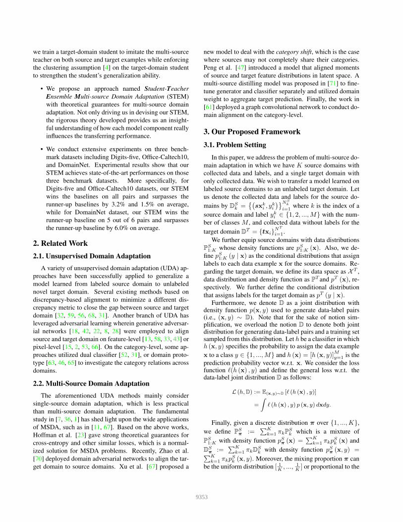
In Table 1, we report the performance of our STEM com-pared with the baselines. Our STEM outperforms the base-lines on all transfer tasks. As far as we know, LtC-MSDA[61] is the current state-of-the-art on Digits-five. Comparedto this baseline, our STEM significantly surpasses sometransfer tasks, i.e., →mm, →sv, and →sy by sizeable mar-gins of 4.1%, 6.7%, and 4.5% respectively and rank the firston average with a significant gap of 3.2%.

4.1.3 Experimental Results on Office-Caltech10

Office-Caltech10 [17] consists of four domains: Amazon(A), Caltech (C), DSLR (D), and Webcam (W). There areten categories in each domain, and the total number of im-ages is 2, 533. In this experiment, we split the training andtesting set with a ratio of 80% and 20%, respectively, anduse ResNet-101 [20] pre-trained on ImageNet as a back-bone.

In Table 2, we present the results of STEM and the base-lines. Overall, it can be seen that our STEM surpasses thebaselines in all four settings and achieves 98.2% on aver-age. Since the baselines already achieve impressive perfor-mances on all adaptation tasks, it is hard to gain significantimprovements. However, on two adaptation tasks (i.e., →Wand →D), our model yields impressive performances withtwo perfect scores of 100%, while STEM also achieves re-markable improvements on the other tasks.

Standard Methods →W →D →C →A AvgSource

CombineSource-only 99.0 98.3 87.8 86.1 92.8DAN [32] 99.3 98.2 89.7 94.8 95.5

Multi-Source

Source-only 99.1 98.2 85.4 88.7 92.9DAN [32] 99.5 99.1 89.2 91.6 94.8

DCTN [67] 99.4 99.0 90.2 92.7 95.3JAN [35] 99.4 99.4 91.2 91.8 95.5

MEDA [62] 99.3 99.2 91.4 92.9 95.7MCD [52] 99.5 99.1 91.5 92.1 95.6

M3SDA [47] 99.5 99.2 92.2 94.5 96.4CMSS [69] 99.6 99.3 93.7 96.6 97.2

STEM (ours) 100 100 94.2 98.4 98.2Table 2. Classification accuracy (%) on Office-Caltech10 dataset.

4.1.4 Experimental Results on DomainNet

DomainNet was first introduced in [47] and has become themost challenging dataset in MSDA. It consists of around0.6 million images of 345 categories from 6 domains: cli-part (clp), infograph (inf), quickdraw (qdr), real (rel) andsketch (skt). Prominently, the high number of classes andenormous noise in this dataset makes it challenging to gainsatisfactory performances even when training and testingfor supervised classification tasks in an individual domain,especially the infograph domain. Moreover, a significantdifference in the distribution of each domain causes the do-main shift problem when transferring knowledge. For allexperiments on this dataset, we utilize ResNet-101 [20] pre-trained on ImageNet as the backbone.

We compare STEM with the current state-of-the-artmethod which is LtC-MSDA [61]. As shown in Table 3,our STEM exceeds LtC-MSDA on 5 out of 6 transfer taskswith significant improvements of 8.9% on →clp task, 9.4%on →qdr task, and 6.5% on →rel task. Averagely, STEMalso yields an impressive improvement of 6.0%.

4.2. Ablation Study

4.2.1 Latent Space Visualization

The crucial factors for the success of our STEM include (i)the mix-up of target domain and the mixture of source do-mains in the latent space and (ii) the target examples arelocated in their matching classes in the source domains. Tovisually demonstrate why STEM can achieve good perfor-mances, we utilize t-SNE [60] to visualize the representa-tions of target and source examples in the latent space. It isnoticeable that in Figure 3, we visualize the case in whichthe target domain is USPS and the rest serves as source do-mains. As shown in Figure 3 (Left) wherein we visualizethe mixture of source domains and the target domain whenthe model is trained with source domains only. In Figure 3(Right), we show how accurately the target examples matchthe classes in the source domains when training the modelwith STEM approach. It is evident that our STEM forms

9358

Standard Methods →clp →inf →pnt →qdr →rel →skt Avg

Single Best

Source-only 39.6 8.2 33.9 11.8 41.6 23.1 26.4DAN [32] 39.1 11.4 33.3 16.2 42.1 29.7 28.6RTN [34] 35.3 10.7 31.7 13.1 40.6 26.5 26.3JAN [35] 35.3 9.1 32.5 14.3 43.1 25.7 26.7

DANN [14] 37.9 11.4 33.9 13.7 41.5 28.6 27.8ADDA [58] 39.5 14.5 29.1 14.9 41.9 30.7 28.4MCD [52] 42.6 19.6 42.6 3.8 50.5 33.8 32.2

SourceCombine

Source-only 47.6 13.0 38.1 13.3 51.9 33.7 32.9DAN [32] 45.4 12.8 36.2 15.3 48.6 34.0 32.1RTN [34] 44.2 12.6 35.3 14.6 48.4 31.7 31.1JAN [35] 40.9 11.1 35.4 12.1 45.8 32.3 29.6

DANN [14] 45.5 13.1 37.0 13.2 48.9 31.8 32.6ADDA [58] 47.5 11.4 36.7 14.7 49.1 33.5 32.2MCD [52] 54.3 22.1 45.7 7.6 58.4 43.5 38.5

Multi-Source

MDAN [70] 52.4 21.3 46.9 8.6 54.9 46.5 38.4DCTN [67] 48.6 23.5 48.8 7.2 53.5 47.3 38.2

M3SDA [47] 58.6 26.0 52.3 6.3 62.7 49.5 42.6MDDA [71] 59.4 23.8 53.2 12.5 61.8 48.6 43.2CMSS [69] 64.2 28.0 53.6 16.0 63.4 53.8 46.5

LtC-MSDA [61] 63.1 28.7 56.1 16.3 66.1 53.8 47.4STEM (ours) 72.0 28.2 61.5 25.7 72.6 60.2 53.4

Table 3. Classification accuracy (%) on DomainNet dataset.

Figure 3. The t-SNE visualization of the transfer task →up withlabel and domain information in two settings: Source-only (left)and our STEM (right). Each color denotes a class while the circleand triangle markers represent the mixture of source and targetdata respectively.

source domains and target domain into the same clustersand the target examples can find their matching classes inthe source domains, hence the label shift is mitigated. Thisexplains the qualified performances of our STEM.

4.2.2 Simplified and Theoretical-Oriented DomainDiscriminator C

We conduct an ablation study to compare two variants ofthe domain discriminator C: theoretical oriented and sim-plified versions (see Section 3.6.1). As shown in Table 4,the simplified variant performs better than the theoreticaloriented one. We conjecture that this is because the sim-plified variant still keeps the principal spirit of the theoret-ically oriented one, while much easier to train due to itssimplicity. Therefore, we select the simplified variant in allexperiments.

Method →mm →mtTheoretical C 86.8 99.1Simplified C 89.7 99.4

Table 4. Comparison of the theoretical oriented and simplified ver-sion of the proposed method

Lvat Lent →mm →up83.04 96.86

! 86.25 96.11! 86.82 97.11

! ! 89.71 98.42Table 5. Ablation study for the affection of VAT and entropy term.

4.2.3 Clustering Assumption Effect

We now speculate the effect of VAT and conditional entropyterms on our model performance. According to Table 5,adding Lvat (first row) or Lent (second row) alone improvesthe performance, while combining these two losses (thirdrow) even boosts the performance further.

Component Digit-five Office-Caltech10 DomainNethS 92.7 97.9 51.6hT 95.0 97.9 53.4

Table 6. The comparison of teacher and student performance.

4.2.4 Teacher and Student Performances

We observe that the performance of the student hT totallydepends on that of the teacher hS . In what follows, we com-pare the performance of the teacher and student on the targetdomain. We report the average of the teacher and student’saccuracy scores for all transfer tasks regarding each dataset.As shown in Table 6, the student outperforms its teacher ex-cept for Office-Caltech10 dataset. This totally makes sensebecause the student not only strictly imitates its teacher, butalso is strengthened the generalization ability by enforcingthe clustering assumption (see Section 3.6.2).

5. ConclusionIn this paper, we propose Student-Teacher Ensemble

Multi-source Domain Adaptation (STEM) for multi-sourcedomain adaptation. Our approach gives strong theoreti-cal guarantees and provides an insightful understanding ofhow each model component really influences the transfer-ring performance. Experiments conducted on three bench-mark datasets, including Digits-five, Office-Caltech10, andDomainNet, demonstrate that our STEM achieves state-of-the-art performances to the best of our knowledge.

AcknowledgementsThis work was supported by the US Air Force grantsFA2386-19-1-4040 and FA9550-19-S-0003.

9359

References[1] S. Ben-David, J. Blitzer, K. Crammer, A. Kulesza,

F. Pereira, and J. W. Vaughan. A theory of learningfrom different domains. Mach. Learn., 79(1-2):151–175, May 2010. 2.2

[2] K. Bousmalis, N. Silberman, D. Dohan, D. Erhan, andD. Krishnan. Unsupervised pixel-level domain adap-tation with generative adversarial networks. In Pro-ceedings of the IEEE conference on computer visionand pattern recognition, pages 3722–3731, 2017. 2.1

[3] Z. Cao, T. Simon, S. Wei, and Y. Sheikh. Real-time multi-person 2d pose estimation using part affin-ity fields. In Proceedings of the IEEE Conferenceon Computer Vision and Pattern Recognition (CVPR),July 2017. 1

[4] O. Chapelle and A. Zien. Semi-supervised classifica-tion by low density separation. In AISTATS, volume2005, pages 57–64. Citeseer, 2005. 1, 3.5, 3.6.2

[5] N. Courty, R. Flamary, A. Habrard, and A. Rakotoma-monjy. Joint distribution optimal transportation fordomain adaptation. In Advances in Neural Informa-tion Processing Systems, pages 3730–3739, 2017. 1

[6] N. Courty, R. Flamary, D. Tuia, and A. Rakotoma-monjy. Optimal transport for domain adaptation. IEEEtransactions on pattern analysis and machine intelli-gence, 39(9):1853–1865, 2017. 1

[7] K. Crammer, M. Kearns, and J. Wortman. Learningfrom multiple sources. In B. Scholkopf, J. C. Platt,and T. Hoffman, editors, Advances in Neural Infor-mation Processing Systems 19, pages 321–328. MITPress, 2007. 2.2

[8] N. Dam, Q. Hoang, T. Le, T. D. Nguyen, H. Bui,and D. Phung. Three-player wasserstein gan viaamortised duality. In Proceedings of the Twenty-Eighth International Joint Conference on Artificial In-telligence, IJCAI-19, pages 2202–2208. InternationalJoint Conferences on Artificial Intelligence Organiza-tion, 7 2019. 2.1

[9] B. B. Damodaran, B. Kellenberger, R. Flamary,D. Tuia, and N. Courty. Deepjdot: Deep joint dis-tribution optimal transport for unsupervised domainadaptation. In Computer Vision - ECCV 2018, pages467–483. Springer, 2018. 1

[10] T. P. Dinh and T. H. A. Le. Convex analysis approachto d.c. programming: Theory, algorithm and applica-tions. 1997. 3.3

[11] L. Duan, D. Xu, and S. Chang. Exploiting web imagesfor event recognition in consumer videos: A multi-ple source domain adaptation approach. In 2012 IEEEConference on Computer Vision and Pattern Recogni-tion, pages 1338–1345, 2012. 2.2

[12] G. French, M. Mackiewicz, and M. Fisher. Self-ensembling for visual domain adaptation. In Interna-tional Conference on Learning Representations, 2018.1

[13] Y. Ganin and V. Lempitsky. Unsupervised domainadaptation by backpropagation. In Proceedings of the32nd International Conference on International Con-ference on Machine Learning, 2015. 1, 2.1

[14] Y. Ganin, E. Ustinova, H. Ajakan, P. Germain,H. Larochelle, F. Laviolette, M. Marchand, andV. Lempitsky. Domain-adversarial training of neuralnetworks. J. Mach. Learn. Res., 17(1):2096–2030, jan2016. 4.1.2, 4.1.4

[15] M. Ghifary, W. B. Kleijn, M. Zhang, D. Balduzzi, andW. Li. Deep reconstruction-classification networks forunsupervised domain adaptation. In European Confer-ence on Computer Vision, pages 597–613. Springer,2016. 2.1

[16] B. Gong, K. Grauman, and F. Sha. Connecting the dotswith landmarks: Discriminatively learning domain-invariant features for unsupervised domain adapta-tion. In Proceedings of the 30th International Con-ference on Machine Learning, pages 222–230, 17–19Jun 2013. 1

[17] B. Gong, Y. Shi, F. Sha, and K. Grauman. Geodesicflow kernel for unsupervised domain adaptation.pages 2066–2073, 06 2012. 4.1.3

[18] I. Goodfellow, J. Pouget-Abadie, M. Mirza, B. Xu,D. Warde-Farley, S. Ozair, A. Courville, and Y. Ben-gio. Generative adversarial nets. In Advances in neu-ral information processing systems, pages 2672–2680,2014. 2.1, 3.2, 3.4, 3.5

[19] Y. Grandvalet and Y. Bengio. Semi-supervised learn-ing by entropy minimization. In L. K. Saul, Y. Weiss,and L. Bottou, editors, Advances in Neural Infor-mation Processing Systems 17, pages 529–536. MITPress, 2005. 3.6.2

[20] K. He, X. Zhang, S. Ren, and J. Sun. Deep residuallearning for image recognition. In 2016 IEEE Con-ference on Computer Vision and Pattern Recognition(CVPR), pages 770–778, 2016. 4.1.3, 4.1.4

9360

[21] G. Hinton, O. Vinyals, and J. Dean. Distilling theknowledge in a neural network. In NIPS Deep Learn-ing and Representation Learning Workshop, 2015.3.2, 3.5

[22] Q. Hoang, T. D. Nguyen, T. Le, and D. Phung. Multi-generator gernerative adversarial nets. arXiv preprintarXiv:1708.02556, 2017. 2.1

[23] J. Hoffman, M. Mohri, and N. Zhang. Algorithms andtheory for multiple-source adaptation. In Advancesin Neural Information Processing Systems 31. CurranAssociates, Inc., 2018. 1, 2.2, 3.3, 1, 3.3

[24] J. J. Hull. A database for handwritten text recognitionresearch. IEEE Transactions on Pattern Analysis andMachine Intelligence, 16(5):550–554, 1994. 4.1.2

[25] D. P. Kingma and J. Ba. Adam: A method for stochas-tic optimization. In Yoshua Bengio and Yann Le-Cun, editors, 3rd International Conference on Learn-ing Representations, ICLR 2015, San Diego, CA, USA,May 7-9, 2015, Conference Track Proceedings, 2015.4.1.1

[26] A. Krizhevsky, I. Sutskever, and G. E Hinton. Im-agenet classification with deep convolutional neuralnetworks. In Advances in neural information process-ing systems, pages 1097–1105, 2012. 1

[27] A. Kumar, P. Sattigeri, K. Wadhawan, L. Karlinsky,R. Feris, B. Freeman, and G. Wornell. Co-regularizedalignment for unsupervised domain adaptation. InAdvances in Neural Information Processing Systems31, pages 9345–9356. Curran Associates, Inc., 2018.3.6.2

[28] T. Le, Q. Hoang, H. Vu, T. D. Nguyen, H. Bui, andD. Phung. Learning generative adversarial networksfrom multiple data sources. In Proceedings of theTwenty-Eighth International Joint Conference on Ar-tificial Intelligence, IJCAI-19, pages 2823–2829. In-ternational Joint Conferences on Artificial IntelligenceOrganization, 7 2019. 2.1

[29] T. Le, T. Nguyen, N. Ho, H. Bui, and D. Phung.Lamda: Label matching deep domain adaptation. InICML, 2021. 1

[30] Y. Lecun, L. Bottou, Y. Bengio, and P. Haffner.Gradient-based learning applied to document recog-nition. Proceedings of the IEEE, 86(11):2278–2324,1998. 4.1.2

[31] C. Lee, T. Batra, M. H. Baig, and D. Ulbricht.Sliced wasserstein discrepancy for unsupervised do-main adaptation. In IEEE Conference on Computer

Vision and Pattern Recognition, CVPR, pages 10285–10295. Computer Vision Foundation / IEEE, 2019. 2.1

[32] M. Long, Y. Cao, J. Wang, and M. I. Jordan. Learningtransferable features with deep adaptation networks.In Proceedings of the 32nd International Conferenceon Machine Learning, volume 37 of Proceedings ofMachine Learning Research, pages 97–105, 2015. 1,2.1, 4.1.2, 4.1.3, 4.1.4

[33] M. Long, Z. Cao, J. Wang, and M. I. Jordan. Con-ditional adversarial domain adaptation. In Advancesin Neural Information Processing Systems 31, pages1640–1650. Curran Associates, Inc., 2018. 2.1

[34] M. Long, H. Zhu, J. Wang, and M. I. Jordan. Unsu-pervised domain adaptation with residual transfer net-works. In Advances in Neural Information ProcessingSystems 29, pages 136–144. 2016. 4.1.4

[35] M. Long, H. Zhu, J. Wang, and M. I. Jordan. Deeptransfer learning with joint adaptation networks. InProceedings of the 34th International Conference onMachine Learning - Volume 70, ICML’17, pages2208–2217, 2017. 4.1.2, 4.1.3, 4.1.4

[36] Y. Mansour, M. Mohri, and A. Rostamizadeh. Do-main adaptation with multiple sources. In D. Koller,D. Schuurmans, Y. Bengio, and L. Bottou, editors, Ad-vances in Neural Information Processing Systems 21,pages 1041–1048. 2009. 1, 2.2, 3.3, 1

[37] T. Miyato, S. Maeda, M. Koyama, and S. Ishii. Vir-tual adversarial training: A regularization method forsupervised and semi-supervised learning. IEEE Trans-actions on Pattern Analysis and Machine Intelligence,41(8):1979–1993, Aug 2019. 3.5, 3.6.2

[38] R. Muller, S. Kornblith, and G. E. Hinton. When doeslabel smoothing help? In Advances in Neural Infor-mation Processing Systems, pages 4694–4703, 2019.3.5

[39] Y. Netzer, T. Wang, A. Coates, A. Bissacco, B. Wu,and A. Y. Ng. Reading digits in natural images withunsupervised feature learning. In NIPS Workshop onDeep Learning and Unsupervised Feature Learning2011, 2011. 4.1.2

[40] T. Nguyen, T. Le, H. Zhao, H. Q. Tran, T. Nguyen,and D. Phung. Most: Multi-source domain adaptationvia optimal transport for student-teacher learning. InUAI, 2021. 1

[41] T. Nguyen, T. Le, H. Zhao, H. Q. Tran, T. Nguyen,and D. Phung. Tidot: A teacher imitation learning ap-proach for domain adaptation with optimal transport.In IJCAI, 2021. 1

9361

[42] T. D. Nguyen, T. Le, H. Vu, and D. Phung. Dual dis-criminator generative adversarial nets. In Advancesin Neural Information Processing Systems 29 (NIPS),2017. 2.1

[43] V. Nguyen, T. Le, O. De Vel, P. Montague, J. Grundy,and D. Phung. Dual-component deep domain adapta-tion: A new approach for cross project software vul-nerability detection. In PAKDD, 2020. 2.1

[44] V. Nguyen, T. Le, T. Le, K. Nguyen, O. De Vel,P. Montague, L. Qu, and D. Phung. Deep domainadaptation for vulnerable code function identification.In IJCNN, 2019. 3.6.2

[45] S. J. Pan, I. W. Tsang, J. T. Kwok, and Q. Yang. Do-main adaptation via transfer component analysis. InProceedings of the 21st International Jont Conferenceon Artifical Intelligence, IJCAI’09, pages 1187–1192,2009. 1

[46] Y. Pan, T. Yao, Y. Li, Y. Wang, C. Ngo, and T. Mei.Transferrable prototypical networks for unsuperviseddomain adaptation. In CVPR, pages 2234–2242, 2019.2.1

[47] X. Peng, Q. Bai, X. Xia, Z. Huang, K. Saenko, andB. Wang. Moment matching for multi-source domainadaptation. In Proceedings of the IEEE InternationalConference on Computer Vision, pages 1406–1415,2019. 2.2, 3.3, 4.1.2, 4.1.3, 4.1.4

[48] B. T. Polyak and A. B. Juditsky. Acceleration ofstochastic approximation by averaging. SIAM J. Con-trol Optim., 30(4):838–855, July 1992. 4.1.1

[49] J. Quionero-Candela, M. Sugiyama, A. Schwaighofer,and N. D. Lawrence. Dataset Shift in Machine Learn-ing. The MIT Press, 2009. 1

[50] S. Ren, K. He, R. Girshick, and J. Sun. Faster r-cnn:Towards real-time object detection with region pro-posal networks. In C. Cortes, N. D. Lawrence, D. D.Lee, M. Sugiyama, and R. Garnett, editors, Advancesin Neural Information Processing Systems 28, pages91–99. Curran Associates, Inc., 2015. 1

[51] K. Saito, Y. Ushiku, and T. Harada. Asymmetric tri-training for unsupervised domain adaptation. In Pro-ceedings of the 34th International Conference on Ma-chine Learning, pages 2988–2997. JMLR. org, 2017.1

[52] K. Saito, K. Watanabe, Y. Ushiku, and T. Harada.Maximum classifier discrepancy for unsupervised do-main adaptation. In CVPR, June 2018. 2.1, 4.1.2,4.1.3, 4.1.4

[53] S. Sankaranarayanan, Y. Balaji, Carlos D. Castillo,and R. Chellappa. Generate to adapt: Aligning do-mains using generative adversarial networks. 2018IEEE/CVF Conference on Computer Vision and Pat-tern Recognition, pages 8503–8512, 2018. 2.1

[54] E. Shelhamer, J. Long, and T. Darrell. Fully convo-lutional networks for semantic segmentation. IEEETransactions on Pattern Analysis and Machine Intelli-gence, 39(4):640–651, April 2017. 1

[55] R. Shu, H. H. Bui, H. Narui, and S. Ermon. A DIRT-t approach to unsupervised domain adaptation. InICLR, 2018. 1, 3.6.2

[56] B. Sun and K. Saenko. Deep coral: Correlation align-ment for deep domain adaptation. In Gang Hua andHerve Jegou, editors, Computer Vision – ECCV 2016Workshops, pages 443–450, Cham, 2016. Springer In-ternational Publishing. 2.1, 4.1.2

[57] Ilya Sutskever, James Martens, George Dahl, andGeoffrey Hinton. On the importance of initializa-tion and momentum in deep learning. volume 28of Proceedings of Machine Learning Research, pages1139–1147, Atlanta, Georgia, USA, 17–19 Jun 2013.PMLR. 4.1.1

[58] E. Tzeng, J. Hoffman, K. Saenko, and T. Darrell. Ad-versarial discriminative domain adaptation. In 2017IEEE Conference on Computer Vision and PatternRecognition (CVPR), pages 2962–2971, 2017. 2.1,4.1.2, 4.1.4

[59] E. Tzeng, J. Hoffman, N. Zhang, K. Saenko, andT. Darrell. Deep domain confusion: Maximizing fordomain invariance. CoRR, abs/1412.3474, 2014. 2.1

[60] L. van der Maaten and G. Hinton. Visualizing datausing t-SNE. Journal of Machine Learning Research,9:2579–2605, 2008. 4.2.1

[61] H. Wang, M. Xu, B. Ni, and W. Zhang. Learningto combine: Knowledge aggregation for multi-sourcedomain adaptation. In Computer Vision – ECCV,2020. 2.2, 4.1.1, 4.1.2, 4.1.4

[62] J. Wang, W. Feng, Y. Chen, H. Yu, M. Huang, and P. S.Yu. Visual domain adaptation with manifold embed-ded distribution alignment. Proceedings of the 26thACM international conference on Multimedia, 2018.4.1.3

[63] S. Xie, Z. Zheng, L. Chen, and C. Chen. Learn-ing semantic representations for unsupervised domainadaptation. In Proceedings of the 35th InternationalConference on Machine Learning, volume 80, pages5423–5432. PMLR, 10–15 Jul 2018. 2.1

9362

[64] K. Xu, J. Ba, R. Kiros, K. Cho, A. Courville,R. Salakhudinov, R. Zemel, and Y. Bengio. Show,attend and tell: Neural image caption generation withvisual attention. volume 37 of Proceedings of MachineLearning Research, pages 2048–2057, Lille, France,07–09 Jul 2015. PMLR. 1

[65] M. Xu, H. Wang, B. Ni, Q. Tian, and W. Zhang. Cross-domain detection via graph-induced prototype align-ment. In 2020 IEEE/CVF Conference on ComputerVision and Pattern Recognition, CVPR 2020, Seat-tle, WA, USA, June 13-19, 2020, pages 12352–12361.IEEE, 2020. 2.1

[66] M. Xu, J. Zhang, B. Ni, T. Li, C. Wang, Q. Tian, andW. Zhang. Adversarial domain adaptation with do-main mixup. In The Thirty-Fourth AAAI Conferenceon Artificial Intelligence, pages 6502–6509. AAAIPress, 2020. 2.1

[67] R. Xu, Z. Chen, W. Zuo, J. Yan, and L. Lin. Deepcocktail network: Multi-source unsupervised domainadaptation with category shift. In 2018 IEEE/CVFConference on Computer Vision and Pattern Recog-nition, pages 3964–3973, 2018. 2.2, 4.1.2, 4.1.3, 4.1.4

[68] H. Yan, Yukang Ding, P. Li, Qilong Wang, Yong Xu,and W. Zuo. Mind the class weight bias: Weightedmaximum mean discrepancy for unsupervised domainadaptation. 2017 IEEE Conference on Computer Vi-sion and Pattern Recognition (CVPR), pages 945–954,2017. 2.1

[69] L. Yang, Y. Balaji, S. Lim, and A. Shrivastava. Cur-riculum manager for source selection in multi-sourcedomain adaptation. In Andrea Vedaldi, Horst Bischof,Thomas Brox, and Jan-Michael Frahm, editors, Com-puter Vision – ECCV 2020, pages 608–624, Cham,2020. 4.1.2, 4.1.3, 4.1.4

[70] H. Zhao, S. Zhang, G. Wu, J. M. F. Moura, J. P.Costeira, and G. J Gordon. Adversarial multiplesource domain adaptation. In Advances in Neural In-formation Processing Systems 31, pages 8559–8570.Curran Associates, Inc., 2018. 1, 2.2, 4.1.2, 4.1.4

[71] S. Zhao, G. Wang, S. Zhang, Y. Gu, Y. Li, Z. Song,P. Xu, R. Hu, H. Chai, and K. Keutzer. Multi-sourcedistilling domain adaptation. Proceedings of the AAAIConference on Artificial Intelligence, 34(07):12975–12983, Apr. 2020. 2.2, 4.1.2, 4.1.4

9363