step by step tutorial about metabolomics analysis with ideom
TRANSCRIPT

IDEOM
IDEOM for LCMS-based metabolomics data
processing: A practical tutorial
Dr Darren Creek [email protected]
Prof Michael Barrett
Prof Rainer Brietling
Andris Jankevics
Dr Karl Burgess
...
http://mzmatch.sourceforge.net/ideom.php

IDEOM
Aim: To interpret LCMS metabolomics data in a biological context
1. Untargeted approach (hypothesis generating):
• Are there differences between samples?
• What are the metabolites that differ?
2. Targeted approach (hypothesis testing):
• What happens to metabolites X, Y and Z
Ideom is designed for untargeted analysis, but can be used for both...

Getting started
i. Open the Ideom_v19.xlsb file in Excel To skip the data processing steps, open IDEOM_v19_Demo.xlsb file. This is an average sized dataset with ~6000 features (peaks) imported. For larger datasets (or
slower computers) allow a few seconds for Excel to re-calculate formulas each time you do something. If it is particularly slow consider turning the ‘Calculation’ option to ‘Manual’. Formulas >> Calculation Options >> Manual
If you do this, remember to hit the ‘Calculate’ button each time you change something.
ii. Allow macros to run
(Security Warning>>Options>>Enable Macros)
Note: if the security warning doesn’t appear: click the Office button (i), go to ‘Excel Options’ >> Trust Centre >> Trust
Centre Settings >> Select ‘Disable all macros with notification’
Getting started
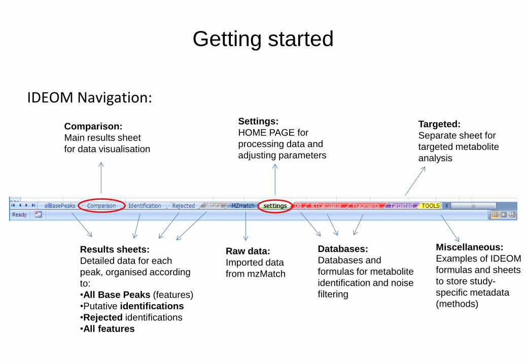
IDEOM Navigation:
Settings:
HOME PAGE for
processing data and
adjusting parameters
Comparison:
Main results sheet
for data visualisation
Results sheets:
Detailed data for each
peak, organised according
to:
•All Base Peaks (features)
•Putative identifications
•Rejected identifications
•All features
Raw data:
Imported data
from mzMatch
Databases:
Databases and
formulas for metabolite
identification and noise
filtering
Miscellaneous:
Examples of IDEOM
formulas and sheets
to store study-
specific metadata
(methods)
Targeted:
Separate sheet for
targeted metabolite
analysis

LCMS Pre-processing
Settings & automated data processing

Part 1
Using IDEOM (and
XCMS/mzMatch) for pre-
processing LCMS
metabolomics data
LCMS Pre-processing
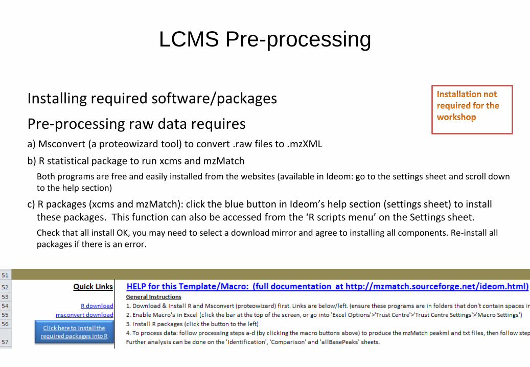
Installing required software/packages
Pre-processing raw data requires a) Msconvert (a proteowizard tool) to convert .raw files to .mzXML
b) R statistical package to run xcms and mzMatch
Both programs are free and easily installed from the websites (available in Ideom: go to the settings sheet and scroll down to the help section)
c) R packages (xcms and mzMatch): click the blue button in Ideom’s help section (settings sheet) to install these packages. This function can also be accessed from the ‘R scripts menu’ on the Settings sheet.
Check that all install OK, you may need to select a download mirror and agree to installing all components. Re-install all packages if there is an error.

LCMS Pre-processing
Raw Data Processing Go to the ‘Settings’ page of Ideom
LCMS Pre-processing
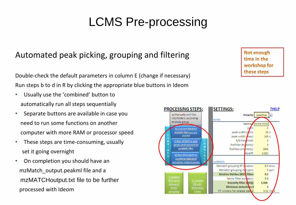
Automated peak picking, grouping and filtering
Double-check the default parameters in column E (change if necessary)
Run steps b to d in R by clicking the appropriate blue buttons in Ideom
• Usually use the ‘combined’ button to
automatically run all steps sequentially
• Separate buttons are available in case you
need to run some functions on another
computer with more RAM or processor speed
• These steps are time-consuming, usually
set it going overnight
• On completion you should have an
mzMatch_output.peakml file and a
mzMATCHoutput.txt file to be further
processed with Ideom
LCMS Pre-processing
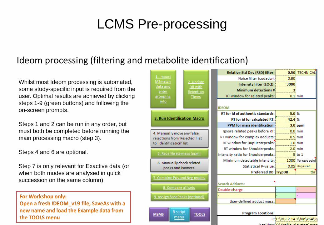
Ideom processing (filtering and metabolite identification)
Whilst most Ideom processing is automated,
some study-specific input is required from the
user. Optimal results are achieved by clicking
steps 1-9 (green buttons) and following the
on-screen prompts.
Steps 1 and 2 can be run in any order, but
must both be completed before running the
main processing macro (step 3).
Steps 4 and 6 are optional.
Step 7 is only relevant for Exactive data (or
when both modes are analysed in quick
succession on the same column)
LCMS Pre-processing
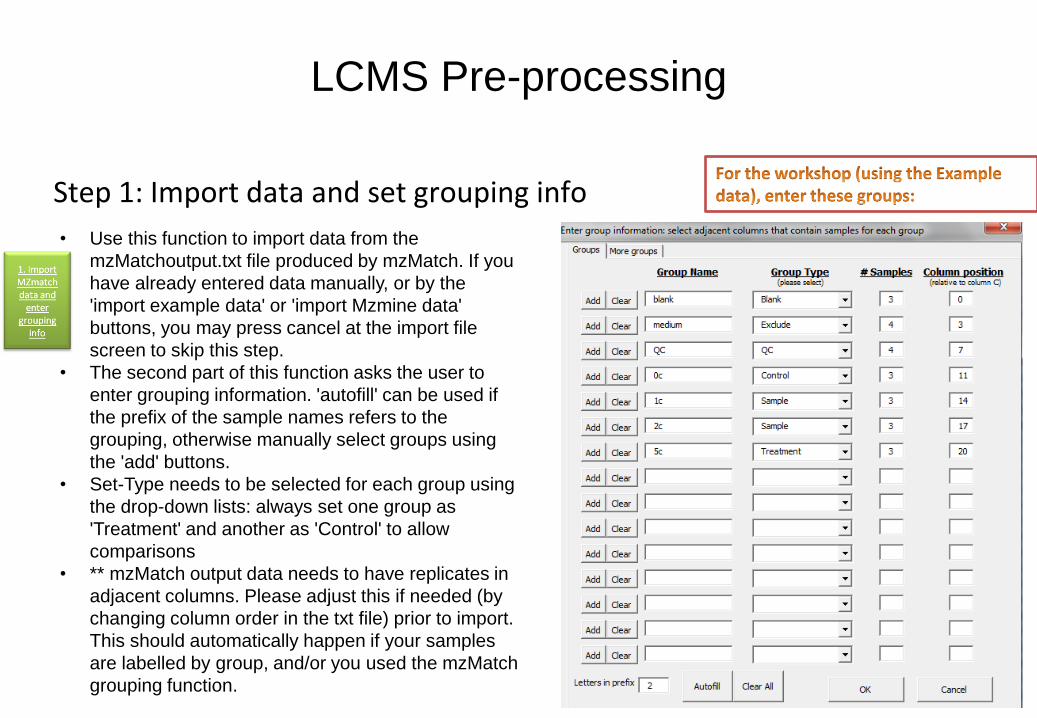
Step 1: Import data and set grouping info
• Use this function to import data from the
mzMatchoutput.txt file produced by mzMatch. If you
have already entered data manually, or by the
'import example data' or 'import Mzmine data'
buttons, you may press cancel at the import file
screen to skip this step.
• The second part of this function asks the user to
enter grouping information. 'autofill' can be used if
the prefix of the sample names refers to the
grouping, otherwise manually select groups using
the 'add' buttons.
• Set-Type needs to be selected for each group using
the drop-down lists: always set one group as
'Treatment' and another as 'Control' to allow
comparisons
• ** mzMatch output data needs to have replicates in
adjacent columns. Please adjust this if needed (by
changing column order in the txt file) prior to import.
This should automatically happen if your samples
are labelled by group, and/or you used the mzMatch
grouping function.
LCMS Pre-processing
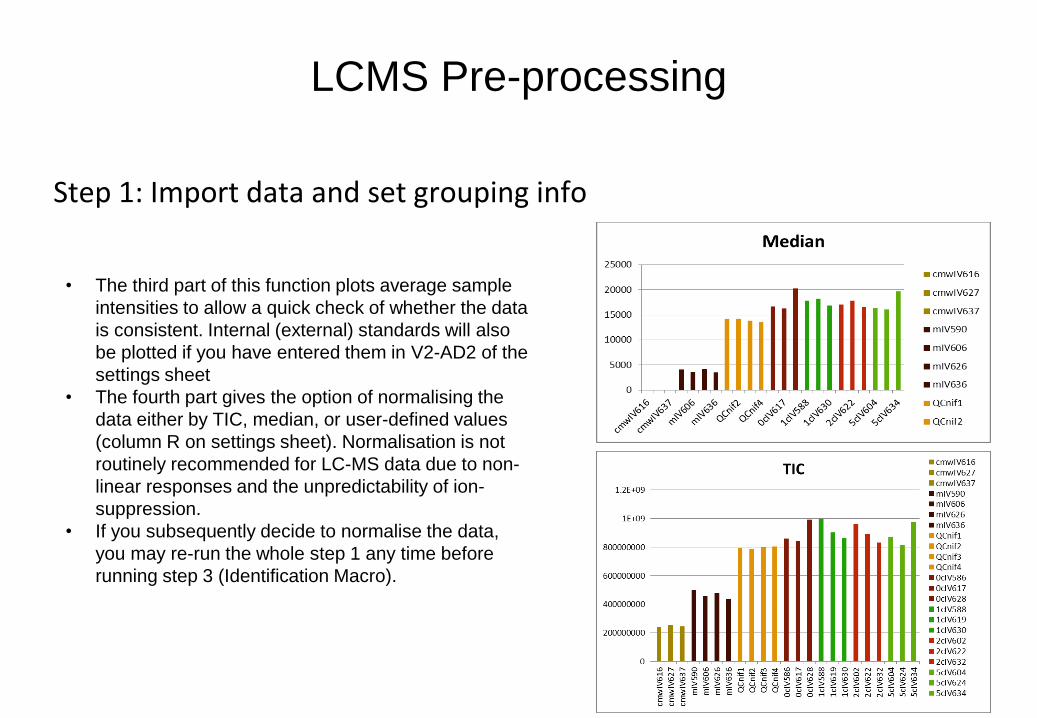
Step 1: Import data and set grouping info
• The third part of this function plots average sample
intensities to allow a quick check of whether the data
is consistent. Internal (external) standards will also
be plotted if you have entered them in V2-AD2 of the
settings sheet
• The fourth part gives the option of normalising the
data either by TIC, median, or user-defined values
(column R on settings sheet). Normalisation is not
routinely recommended for LC-MS data due to non-
linear responses and the unpredictability of ion-
suppression.
• If you subsequently decide to normalise the data,
you may re-run the whole step 1 any time before
running step 3 (Identification Macro).

LCMS Pre-processing
Step 2: Update DB with retention times
• This function enters standard retention times into the database (DB
sheet), and (optional) enters predicted retention times for other
metabolites.
• A list of retention times from authentic standards is required (create this
list either using the Targeted Sheet, or externally using ToxID, Xcalibur
or similar)
• The list of standard RTs may be either imported from any excel readable
file, or entered directly into columns A and B on the 'RTcalculator' sheet
• If importing .csv files of retention times: "_" in metabolite names will be
replaced with ","
• All authentic standards (column A on the 'RTcalculator' sheet) must have
names that exactly match those in the DB sheet.
• RT calculator uses physico-chemical properties in the DB sheet to
predict retention times based on a multiple linear regression model with
the authentic standards. (QSPR approach)
• The column (cell O8) and dead volume time (cell O9) should be entered
before running this macro. Other data in columns N-U show the
accuracy of the current RT prediction model.
• The mass range for application of the prediction model is defined in cells
O10 and Q10. The default QSPR model is accurate for the Formic
Acid:ZIC-HILIC method from MW 70-400

LCMS Pre-processing
Step 2: Update DB with retention times (cont)
• Columns W:X allow standard retention times to be uploaded to the database without being included in the
prediction model. (e.g. for large metabolites outside the validated mass range)
• Columns Z:AI allow predicted retention times to be uploaded to the database based on class properties,
according to specific annotations in the DB sheet (if no RT calculated by the prediction model)
• Prediction model variables (Headers E1:J1) can be adjusted to other phys-chem properties (from drop-down
menus) if you wish to attempt to apply RT prediction to different chromatography.
• You have the opportunity to check the model fit before annotating all metabolites in the database.
• If there is no good prediction model you can still use this function to upload standard retention times for
those metabolites where you have authentic standards.
• If you don't run this function then metabolite identification will only be based on exact mass (not retention
time) - hence you will get a lot more false-identifications.
LCMS Pre-processing
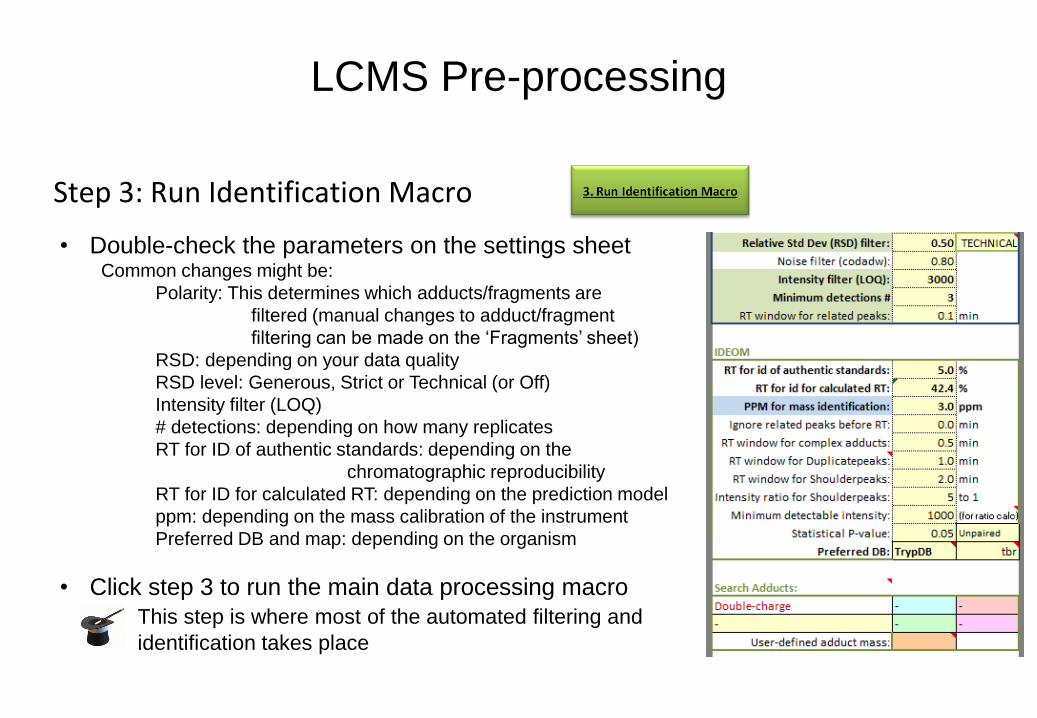
Step 3: Run Identification Macro
• Double-check the parameters on the settings sheet Common changes might be:
Polarity: This determines which adducts/fragments are
filtered (manual changes to adduct/fragment
filtering can be made on the ‘Fragments’ sheet)
RSD: depending on your data quality
RSD level: Generous, Strict or Technical (or Off)
Intensity filter (LOQ)
# detections: depending on how many replicates
RT for ID of authentic standards: depending on the
chromatographic reproducibility
RT for ID for calculated RT: depending on the prediction model
ppm: depending on the mass calibration of the instrument
Preferred DB and map: depending on the organism
• Click step 3 to run the main data processing macro
This step is where most of the automated filtering and
identification takes place

LCMS Pre-processing
Step 4: Manually retrieve False Rejections
• Check the rejected sheet for metabolites that you believe to be wrongly rejected
If you think a metabolite was wrongly rejected:
Check if the metabolite has already been identified (as another feature) by double-clicking the confidence level
(in column F)
If you can justify why a feature was incorrectly rejected: retrieve the metabolite by clicking the red ‘Retrieve
Row’ button at the top
E.g. In example data find Folate (which was rejected because it appears to be a dimer of another peak).

LCMS Pre-processing
Step 5: Recalibrate mass (ppm)
• Go to the Identification sheet or the settings page
• Run step 5 by clicking the green ‘re-calibrate mass (ppm
check)’ button • This will plot the relationship between mass and mass accuracy
(ppm error) for all 'identified' metabolites, with standards in red, and
fit a 5th order polynomial function. (this should allow for the
calibration errors observed on Thermo Orbitrap)
• If the polynomial function appears to fit your data, agree to re-
calibrate masses. If the curve is not a good fit, but you see a trend,
consider manual re-calibration efforts.
• After calibration, check the new plot of mass errors, and set a new
ppm window to remove outliers (false-identifications). In some cases
it is worth checking the rejected peaks (bottom of 'rejected' list) for
alternative identifications by clicking the 'altppm' column
LCMS Pre-processing
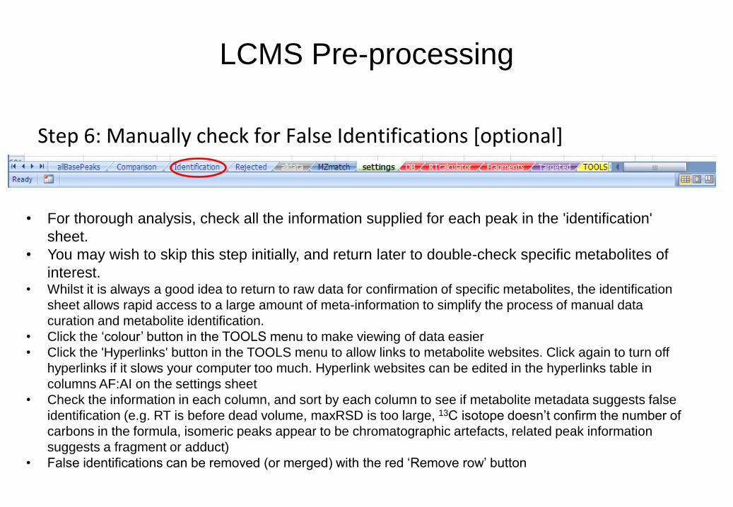
Step 6: Manually check for False Identifications [optional]
• For thorough analysis, check all the information supplied for each peak in the 'identification'
sheet.
• You may wish to skip this step initially, and return later to double-check specific metabolites of
interest. • Whilst it is always a good idea to return to raw data for confirmation of specific metabolites, the identification
sheet allows rapid access to a large amount of meta-information to simplify the process of manual data
curation and metabolite identification.
• Click the ‘colour’ button in the TOOLS menu to make viewing of data easier
• Click the 'Hyperlinks' button in the TOOLS menu to allow links to metabolite websites. Click again to turn off
hyperlinks if it slows your computer too much. Hyperlink websites can be edited in the hyperlinks table in
columns AF:AI on the settings sheet
• Check the information in each column, and sort by each column to see if metabolite metadata suggests false
identification (e.g. RT is before dead volume, maxRSD is too large, 13C isotope doesn’t confirm the number of
carbons in the formula, isomeric peaks appear to be chromatographic artefacts, related peak information
suggests a fragment or adduct)
• False identifications can be removed (or merged) with the red ‘Remove row’ button

LCMS Pre-processing
Add Chromatograms
• Add EICs to column A of the ‘Identification’ sheet by the ‘Add Chromatograms’ button
• This function requires access to the corresponding peakml file. NB: chromatograms are uploaded
based on the peakID number. Therefore, take care to use only the peakml file that corresponds to
the data matrix (mzMatchoutput.txt) uploaded to IDEOM.
• Alternatively (if your computer cannot load the peakml file) the chromatogram images can be
generated from a peakml file on any machine using the R script available on the ‘settings’ sheet
(this folder of chromatogram images is generated by the default script in step d)
• You may run this step on any results sheet at any time
(e.g. Identification, Comparison, allBasepeaks)
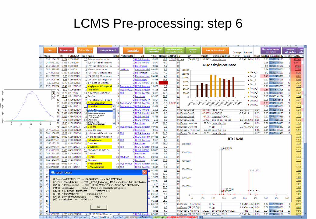
LCMS Pre-processing: step 6
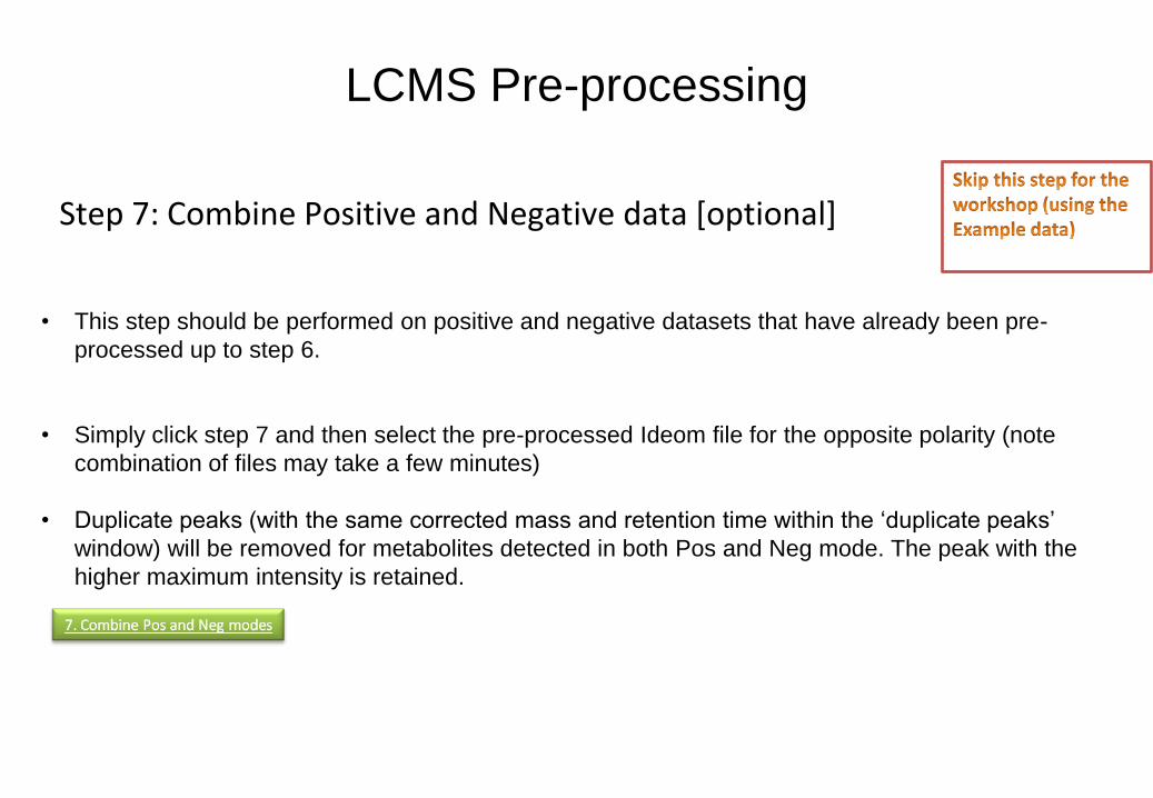
LCMS Pre-processing
Step 7: Combine Positive and Negative data [optional]
• This step should be performed on positive and negative datasets that have already been pre-
processed up to step 6.
• Simply click step 7 and then select the pre-processed Ideom file for the opposite polarity (note
combination of files may take a few minutes)
• Duplicate peaks (with the same corrected mass and retention time within the ‘duplicate peaks’
window) will be removed for metabolites detected in both Pos and Neg mode. The peak with the
higher maximum intensity is retained.

LCMS Pre-processing
Step 8: Compare all sets
Step 9: Assign Basepeaks [optional]
• Run this function to summarise data into the Comparison sheet
• You have the option to only include the identified peaks, or to also include all significant base
peaks (including unidentified and those with low identity confidence)
• This step can be repeated as required for different ‘control’ groups or with/without basepeaks
• Sometimes base peaks are actually a related peak (adduct/fragment) of a smaller peak. This
function takes all unidentified base peaks and annotates them if any related peaks have been
(putatively) identified.
• This step could be run before step 8 if you want this information in the Comparison sheet
Ideom Tutorial: Part 2
Data Interpretation/Visualization Tutorial plan • Getting Started
• Finding differences - sort
- filter
- graph
• Checking data integrity “Is it a real difference”
• Metabolite Identification
• Exporting to external programs or websites
• Changing groups for comparison

Getting started
Select the ‘Comparison’ sheet
Scroll up and down to see the list of metabolites
- Metabolites (column E) highlighted yellow have been identified with authentic standards, all other
metabolites are putatively identified from the database
- Red names (column E) indicate more than one peak has been identified as that metabolite
- Formula’s (column C) in red text indicate more than one peak is present with that formula (i.e. isomers... or shoulder peaks)
- Masses (column A) are highlighted according to the polarity mode of detection:
- Red = positive ionisation
- Blue = negative ionisation
- White = detected in both positive and negative modes
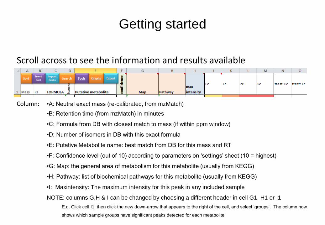
Getting started
Scroll across to see the information and results available
Column: •A: Neutral exact mass (re-calibrated, from mzMatch)
•B: Retention time (from mzMatch) in minutes
•C: Formula from DB with closest match to mass (if within ppm window)
•D: Number of isomers in DB with this exact formula
•E: Putative Metabolite name: best match from DB for this mass and RT
•F: Confidence level (out of 10) according to parameters on ‘settings’ sheet (10 = highest)
•G: Map: the general area of metabolism for this metabolite (usually from KEGG)
•H: Pathway: list of biochemical pathways for this metabolite (usually from KEGG)
•I: Maxintensity: The maximum intensity for this peak in any included sample
NOTE: columns G,H & I can be changed by choosing a different header in cell G1, H1 or I1
E.g. Click cell I1, then click the new down-arrow that appears to the right of the cell, and select ‘groups’. The column now
shows which sample groups have significant peaks detected for each metabolite.
Getting started
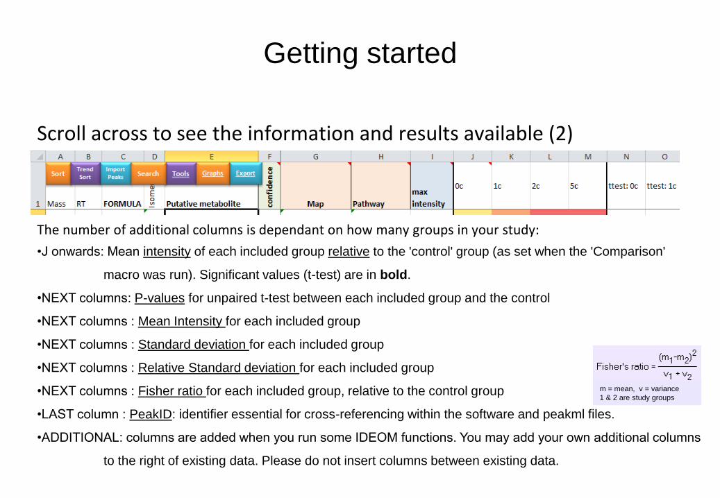
Scroll across to see the information and results available (2)
The number of additional columns is dependant on how many groups in your study:
•J onwards: Mean intensity of each included group relative to the 'control' group (as set when the 'Comparison'
macro was run). Significant values (t-test) are in bold.
•NEXT columns: P-values for unpaired t-test between each included group and the control
•NEXT columns : Mean Intensity for each included group
•NEXT columns : Standard deviation for each included group
•NEXT columns : Relative Standard deviation for each included group
•NEXT columns : Fisher ratio for each included group, relative to the control group
•LAST column : PeakID: identifier essential for cross-referencing within the software and peakml files.
•ADDITIONAL: columns are added when you run some IDEOM functions. You may add your own additional columns
to the right of existing data. Please do not insert columns between existing data.
m = mean, v = variance
1 & 2 are study groups
Ideom Tutorial: Part 2
Data Interpretation/Visualization Tutorial plan • Getting Started
• Finding differences - sort
- filter
- graph
• Checking data integrity “Is it a real difference”
• Metabolite Identification
• Exporting to external programs or websites
• Changing groups for comparison

Finding differences
Sort by specific columns to find the most changing metabolites
Fold-change 0c is currently set as the ‘control’.
To find the differences between 1c and 0c, sort by ‘1c’ (column K)
1. Sort using the orange ‘Sort’ button at the top-left and follow the instructions
(If using the inbuilt Excel sort or autofilter function please double-check that all data is selected)
1
Finding differences
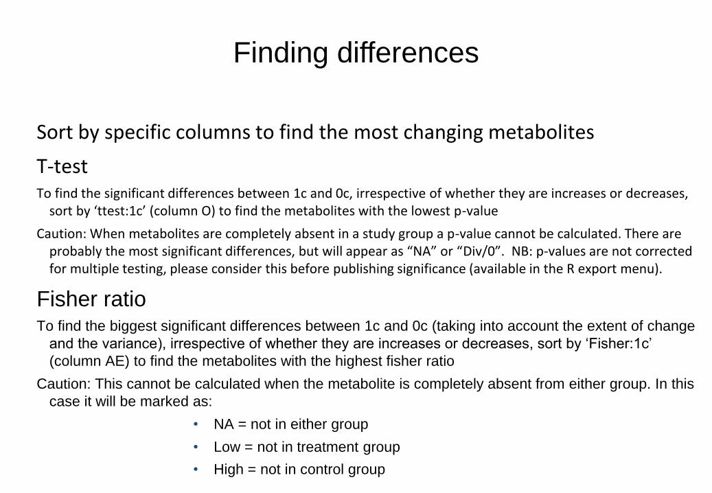
Sort by specific columns to find the most changing metabolites
T-test To find the significant differences between 1c and 0c, irrespective of whether they are increases or decreases,
sort by ‘ttest:1c’ (column O) to find the metabolites with the lowest p-value
Caution: When metabolites are completely absent in a study group a p-value cannot be calculated. There are probably the most significant differences, but will appear as “NA” or “Div/0”. NB: p-values are not corrected for multiple testing, please consider this before publishing significance (available in the R export menu).
Fisher ratio To find the biggest significant differences between 1c and 0c (taking into account the extent of change
and the variance), irrespective of whether they are increases or decreases, sort by ‘Fisher:1c’
(column AE) to find the metabolites with the highest fisher ratio
Caution: This cannot be calculated when the metabolite is completely absent from either group. In this
case it will be marked as:
• NA = not in either group
• Low = not in treatment group
• High = not in control group

Finding differences
Sort by specific columns to find the most changing metabolites
Other columns It is less meaningful to sort by the “mean” columns, because LCMS response is different for every metabolite.
For example, two metabolites with the same concentration could give 1000-fold different LCMS peak intensities due to their differing ionisation properties.
You may wish to combine sorting by differences with sorting by pathway (or other metabolite properties) to assist with interpretation.

Finding differences
Z-transformation
Z-transformation is performed on all samples to
express variance relative to the standard
deviations from the mean of the control group
Data will be added to columns to the right of
existing data
Finding differences
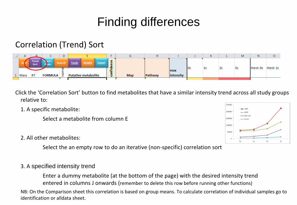
Correlation (Trend) Sort
Click the ‘Correlation Sort’ button to find metabolites that have a similar intensity trend across all study groups
relative to:
1. A specific metabolite:
Select a metabolite from column E
2. All other metabolites:
Select the an empty row to do an iterative (non-specific) correlation sort
3. A specified intensity trend
Enter a dummy metabolite (at the bottom of the page) with the desired intensity trend entered in columns J onwards (remember to delete this row before running other functions)
NB: On the Comparison sheet this correlation is based on group means. To calculate correlation of individual samples go to identification or alldata sheet.

Finding differences
Correlation Matrix
Click the ‘Correlation Matrix’ button in the TOOLS
menu to find the cross-correlation of intensities between metabolites.
Pearson correlation coefficients will be written to a new worksheet and coloured in a heatmap format.
CAUTION: Metabolites with very high correlation may actually be LCMS artefacts that escaped the filtering steps. Double-check these by analysis of retention times.

Filtering your list
Excel’s Autofilter function is a very useful way to tidy your dataset to optimise visualisation, graphing or export functions for your metabolites of interest
1. Activate the filter (if it is not already activated)
2. Click on the down-arrow for the column you wish to
filter by
3. Filter by selecting/deselecting the checkboxes, or set
a number, color or custom filter
Examples:
Filter by Confidence > 6 (to get more confident ID’s)
Filter by specific maps/pathways, or by “Text that contains”: Lipid
Filter by P-value < 0.01 for a specific study group
Filter by maxintensity > 10,000, or in Groups “text that contains”:
5c
Filter name by color to see only metabolites identified with
authentic standards
1
2
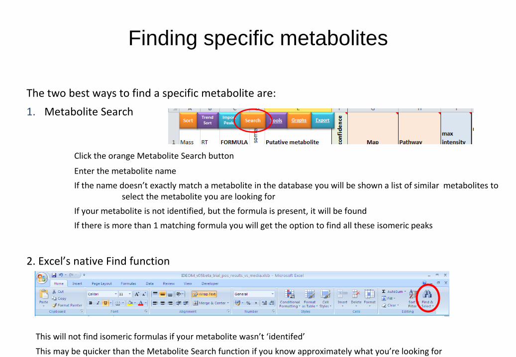
The two best ways to find a specific metabolite are:
1. Metabolite Search
Click the orange Metabolite Search button
Enter the metabolite name
If the name doesn’t exactly match a metabolite in the database you will be shown a list of similar metabolites to select the metabolite you are looking for
If your metabolite is not identified, but the formula is present, it will be found
If there is more than 1 matching formula you will get the option to find all these isomeric peaks
2. Excel’s native Find function
This will not find isomeric formulas if your metabolite wasn’t ‘identifed’
This may be quicker than the Metabolite Search function if you know approximately what you’re looking for
Finding specific metabolites
Graphing
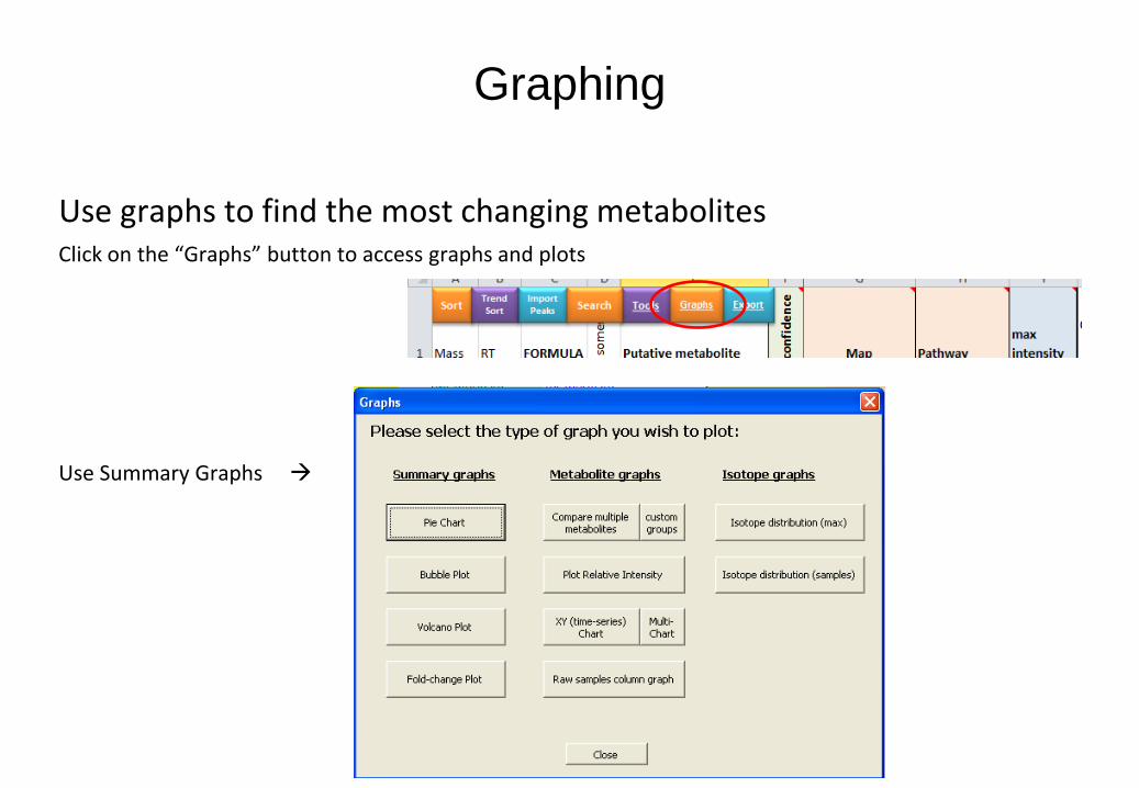
Use graphs to find the most changing metabolites Click on the “Graphs” button to access graphs and plots
Use Summary Graphs

Graphing
Summary graphs: Bubble plot Click the bubble plot to see the metabolites according to their detected masses and retention times. Larger
bubbles represent larger relative intensities (compared to the control group)
•Edit graph as you would for
any graph in Excel.
•If only interested in 0c and 5c,
delete the extra series (click on
the bubbles and press delete,
or right click and ‘Select Data’)
•Make it bigger/smaller to suit
•Hover mouse over any point
to get details of the retention
time, mass and relative
intensity
•Click the X in the corner to
close (or select the graph and
press delete)
Graphing
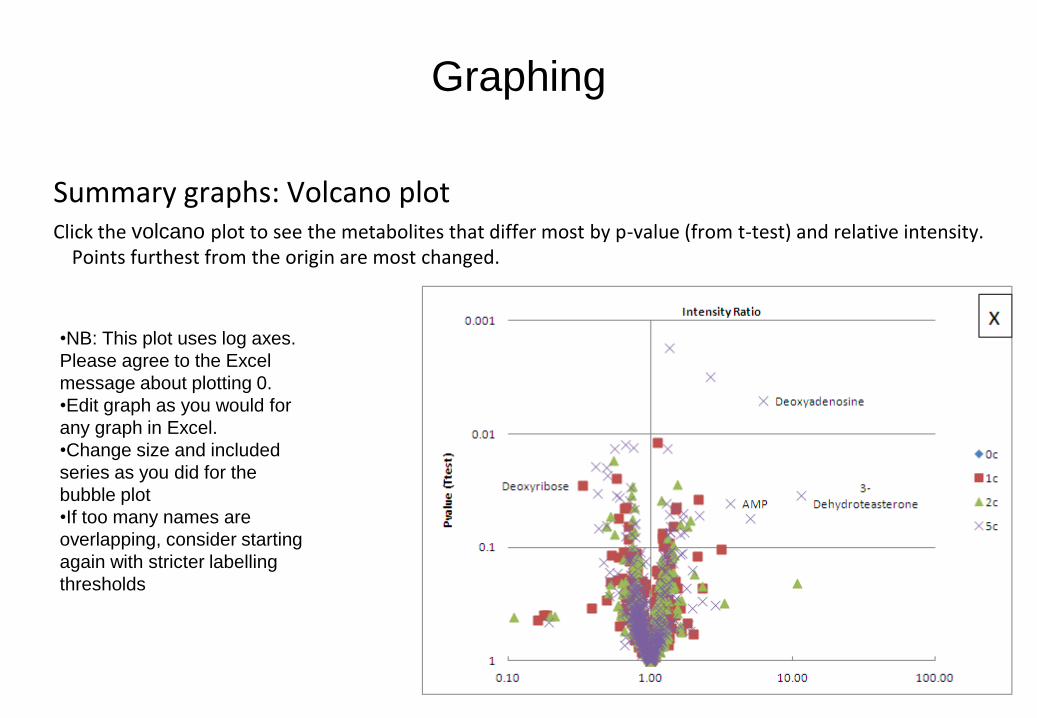
Summary graphs: Volcano plot Click the volcano plot to see the metabolites that differ most by p-value (from t-test) and relative intensity.
Points furthest from the origin are most changed.
•NB: This plot uses log axes.
Please agree to the Excel
message about plotting 0.
•Edit graph as you would for
any graph in Excel.
•Change size and included
series as you did for the
bubble plot
•If too many names are
overlapping, consider starting
again with stricter labelling
thresholds

Graphing
Summary graphs: Fold-change plot Click the Fold-change plot to see the relative intensity of all metabolites separately, or grouped by pathway.
This looks better if you have fewer metabolites.
•NB: This plot uses log axes.
Please agree to the Excel
message about plotting 0.
•Edit graph as you would for
any graph in Excel.
•Change size and included
series as you did for the
bubble plot
•If you grouped by pathway, try
again by plotting all
metabolites
•If too many names are
overlapping, consider filtering
the list beforehand

Graphing
Summary graphs Click the Pie chart button to see a distribution of your identified metabolites (this doesn’t give any information
about changing metabolite levels). (NOTE: the pie chart is the only graph in Ideom that cannot handle filtered data)

Ideom Tutorial: Part 2
Data Interpretation/Visualization Tutorial plan • Getting Started
• Finding differences - sort
- filter
- graph
• Checking data integrity “Is it a real difference”
• Metabolite Identification
• Exporting to external programs or websites
• Changing groups for comparison

Checking differences
Is the difference real? Means, standard deviations, t-tests and fisher ratios for each metabolite are available.
Graphs for individual metabolites are the best way to see differences:
• Double-click a metabolite name: this gives a column chart with mean peak intensity and standard deviations as error bars
• Double-click a specific cell in column I: this gives a column chart showing the peak intensity for every individual sample. Each sample is coloured according to it’s study group

Checking differences
Is the difference real? Additional graphs for individual metabolites are available from the ‘Graphing’ button:

Checking differences
Technical note on copying graphs It is often nice to copy Ideom charts to a Word or Powerpoint file for reports or presentation
Be careful… Office links charts, so that if you do further processing in Ideom (i.e. sorting or filtering) the chart in Word/Powerpoint will change without you knowing!!
Two ways to avoid this are:
1. After pasting the chart in Word/Powerpoint ‘break the link’ to the Excel chart
2007: Office button >> Prepare >> Edit links to files >> select chart and click ‘Break link’
2010: Office button >> File >> Edit links to files >> select chart and click ‘Break link’
2. Paste as a picture (however in this case you can’t edit it later)
Paste special >> picture (PNG)
Troubleshooting:
If you have trouble copying a chart, deselect it (by selecting another random cell), then select it again
and then copy.

Checking differences
Is the difference real…? Ion suppression? Occasionally in LCMS an intensity difference is apparent for one metabolite, which is actually due to altered
ionisation (enhanced or suppressed) caused by another chemical (metabolite, salt, solvent, or contaminant).
Internal standards
The best way to avoid this problem is to use isotope-labelled internal standards for every metabolite to normalise peak intensities. (see new features later in this tutorial)
External standards
Ideom currently supports inclusion of up to 9 external standards for quality control purposes (see Settings sheet). Intensities for these is plotted for each sample (if present) on the mzMatch page(s) after uploading data from mzMatch. Normalisation by these standards is not recommended (unless one of them co-elutes with your metabolite of interest).
Sort by retention time
Sort your results by retention time (column B), and if there are numerous co-eluting compounds (i.e. with similar retention times) that show the same intensity trend across sample groups then your differences may be due to ion suppression.

Checking differences
Is the difference real…? Show me the data! For absolute confirmation (i.e. before publishing a significant finding), double-check the peaks in raw data: (in
case the intensity difference is due to odd peak shapes, or a peak was missed or not grouped correctly in the data processing)
Mouse-over cells in column A to see the extracted chromatograms
Double-click the retention time for a specific metabolite (in column B):
This gives you a graph showing the retention time and intensities of all peaks with the same mass
Alternatively (not in tutorial):
• Ctrl-Shift-X : activates the macro to view a selected mass in Xcalibur (mass must be selected first)

Ideom Tutorial: Part 2
Data Interpretation/Visualization Tutorial plan • Getting Started
• Finding differences - sort
- filter
- graph
• Checking data integrity “Is it a real difference”
• Metabolite Identification
• Exporting to external programs or websites
• Changing groups for comparison
Metabolite Identification
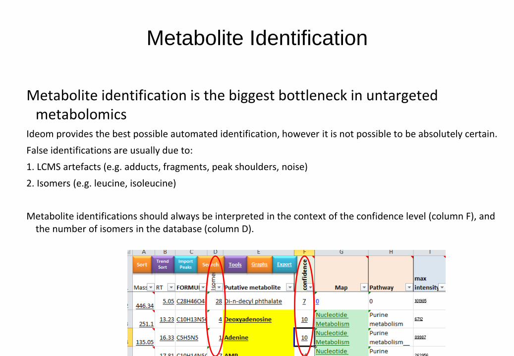
Metabolite identification is the biggest bottleneck in untargeted metabolomics
Ideom provides the best possible automated identification, however it is not possible to be absolutely certain.
False identifications are usually due to:
1. LCMS artefacts (e.g. adducts, fragments, peak shoulders, noise)
2. Isomers (e.g. leucine, isoleucine)
Metabolite identifications should always be interpreted in the context of the confidence level (column F), and the number of isomers in the database (column D).

Metabolite Identification
Identification verification
1. Confidence score and information box
2. Related Peaks (MS artefacts)
3. Isomers
4. EIC: Other peaks in the chromatogram
5. Alternate formulas (including adducts)
6. Sample intensities and reproducibility
7. Peak shape
8. Presence of associated metabolites (KEGG pathways)

Metabolite Identification
1. Confidence score and information box The confidence level (column F) gives an indication of the confidence of identification.
Double-click a cell in column F to get background information about each metabolite to help confirm or reject the identification (e.g. find L-Tyrosine and double-click on the 8 in column F)
This metabolite is identified as L-Tyrosine according to the formula, but there are 11
possible isomers.
L-Tyrosine is expected in these samples according to the KEGG Tbr annotations,
and this metabolite is in MetaCyc and HMDB.
The detected mass is correct for this formula within 0.75ppm and it was detected in
both pos and neg ionisation, predominantly as the protonated adduct.
The retention time is 3.3% earlier than the authentic standard RT.
mzMatch suggests this is related to L-Valine, but the mass difference is 63.9948,
which is not a likely adduct.
The C13 isotope confirms the presence of 9 carbon atoms (-0.4% error), and there is
also an O18 isotope (confirming oxygen atoms are present). Fragments for loss of
ammonium and loss of formic acid are consistent with this metabolite containing a
primary amine and carboxylic acid.
The maximum peak intensity is 12727400, which is large (i.e. it is not background
noise), and the maximum RSD is 0.47 (i.e. Some variability in some samples), but
the QC samples are reproducible (RSD: 0.08). This peak is found at significant
levels in all study groups (0c, 1c, 2c and 5c).
In summary, it is highly likely that this peak is indeed L-Tyrosine, but to be absolutely
certain you would need to rule out the 10 other possible isomers
NOTE: This information is stored in the ‘Identification’ sheet. Change the header in column I to access this information directly on the ‘comparison’ sheet.

Metabolite Identification
2. Check Related Peaks To see the mass spectra of all co-eluting peaks double-click the mass (column A)
The green peak is this peak. The red peaks are related (according to mzMatch). The blue peaks are co-eluting, but probably not related.
Example: Double-click the
mass for L-Tyrosine.
Hover over a mass in the
graph to see annotations
and click to go to the
‘alldata’ sheet to
interrogate these peaks in
detail
NOTE: This is the only Ideom graph
that cannot be easily re-sized. The
MS peaks do not move to scale with
the axes.
Metabolite Identification
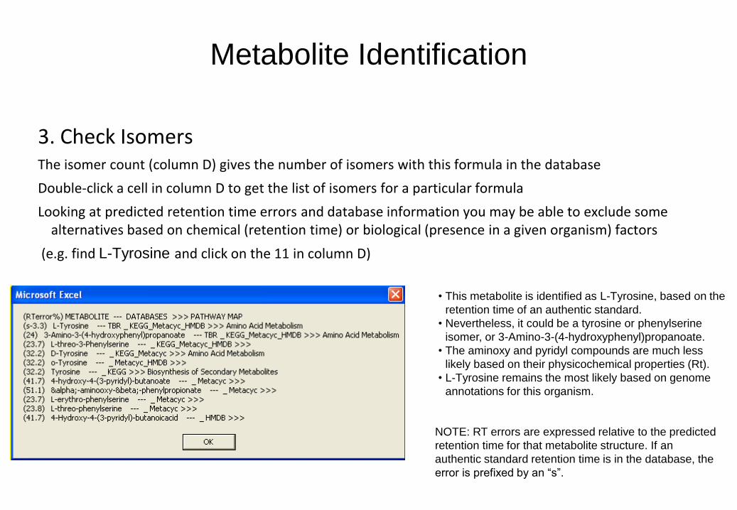
3. Check Isomers The isomer count (column D) gives the number of isomers with this formula in the database
Double-click a cell in column D to get the list of isomers for a particular formula
Looking at predicted retention time errors and database information you may be able to exclude some alternatives based on chemical (retention time) or biological (presence in a given organism) factors
(e.g. find L-Tyrosine and click on the 11 in column D)
• This metabolite is identified as L-Tyrosine, based on the
retention time of an authentic standard.
• Nevertheless, it could be a tyrosine or phenylserine
isomer, or 3-Amino-3-(4-hydroxyphenyl)propanoate.
• The aminoxy and pyridyl compounds are much less
likely based on their physicochemical properties (Rt).
• L-Tyrosine remains the most likely based on genome
annotations for this organism.
NOTE: RT errors are expressed relative to the predicted
retention time for that metabolite structure. If an
authentic standard retention time is in the database, the
error is prefixed by an “s”.
Metabolite Identification
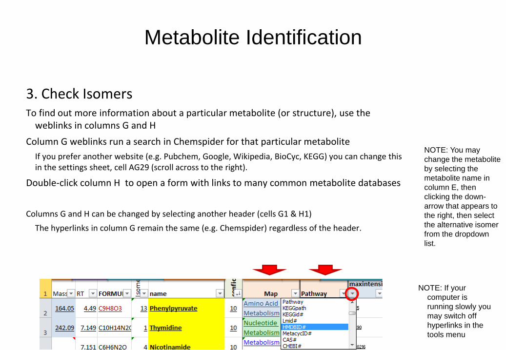
3. Check Isomers To find out more information about a particular metabolite (or structure), use the
weblinks in columns G and H
Column G weblinks run a search in Chemspider for that particular metabolite
If you prefer another website (e.g. Pubchem, Google, Wikipedia, BioCyc, KEGG) you can change this in the settings sheet, cell AG29 (scroll across to the right).
Double-click column H to open a form with links to many common metabolite databases
Columns G and H can be changed by selecting another header (cells G1 & H1)
The hyperlinks in column G remain the same (e.g. Chemspider) regardless of the header.
NOTE: If your
computer is
running slowly you
may switch off
hyperlinks in the
tools menu
NOTE: You may
change the metabolite
by selecting the
metabolite name in
column E, then
clicking the down-
arrow that appears to
the right, then select
the alternative isomer
from the dropdown
list.
Metabolite Identification
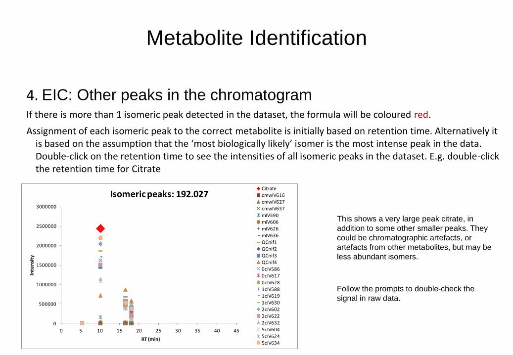
4. EIC: Other peaks in the chromatogram If there is more than 1 isomeric peak detected in the dataset, the formula will be coloured red.
Assignment of each isomeric peak to the correct metabolite is initially based on retention time. Alternatively it is based on the assumption that the ‘most biologically likely’ isomer is the most intense peak in the data. Double-click on the retention time to see the intensities of all isomeric peaks in the dataset. E.g. double-click the retention time for Citrate
This shows a very large peak citrate, in
addition to some other smaller peaks. They
could be chromatographic artefacts, or
artefacts from other metabolites, but may be
less abundant isomers.
0
500000
1000000
1500000
2000000
2500000
3000000
0 5 10 15 20 25 30 35 40 45
Inte
nsi
ty
RT (min)
Isomeric peaks: 192.027CitratecmwIV616cmwIV627cmwIV637mIV590mIV606mIV626mIV636QCnif1QCnif2QCnif3QCnif40cIV5860cIV6170cIV6281cIV5881cIV6191cIV6302cIV6022cIV6222cIV6325cIV6045cIV6245cIV634
Follow the prompts to double-check the
signal in raw data.
Metabolite Identification
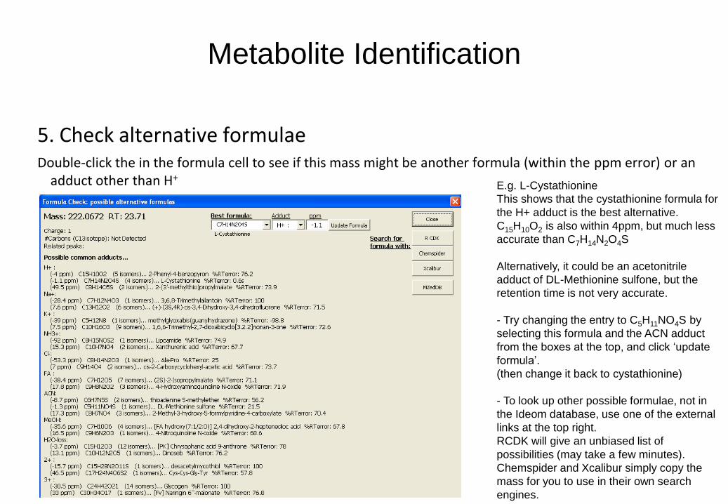
5. Check alternative formulae Double-click the in the formula cell to see if this mass might be another formula (within the ppm error) or an
adduct other than H+
E.g. L-Cystathionine
This shows that the cystathionine formula for
the H+ adduct is the best alternative.
C15H10O2 is also within 4ppm, but much less
accurate than C7H14N2O4S
Alternatively, it could be an acetonitrile
adduct of DL-Methionine sulfone, but the
retention time is not very accurate.
- Try changing the entry to C5H11NO4S by
selecting this formula and the ACN adduct
from the boxes at the top, and click ‘update
formula’.
(then change it back to cystathionine)
- To look up other possible formulae, not in
the Ideom database, use one of the external
links at the top right.
RCDK will give an unbiased list of
possibilities (may take a few minutes).
Chemspider and Xcalibur simply copy the
mass for you to use in their own search
engines.
Metabolite Identification
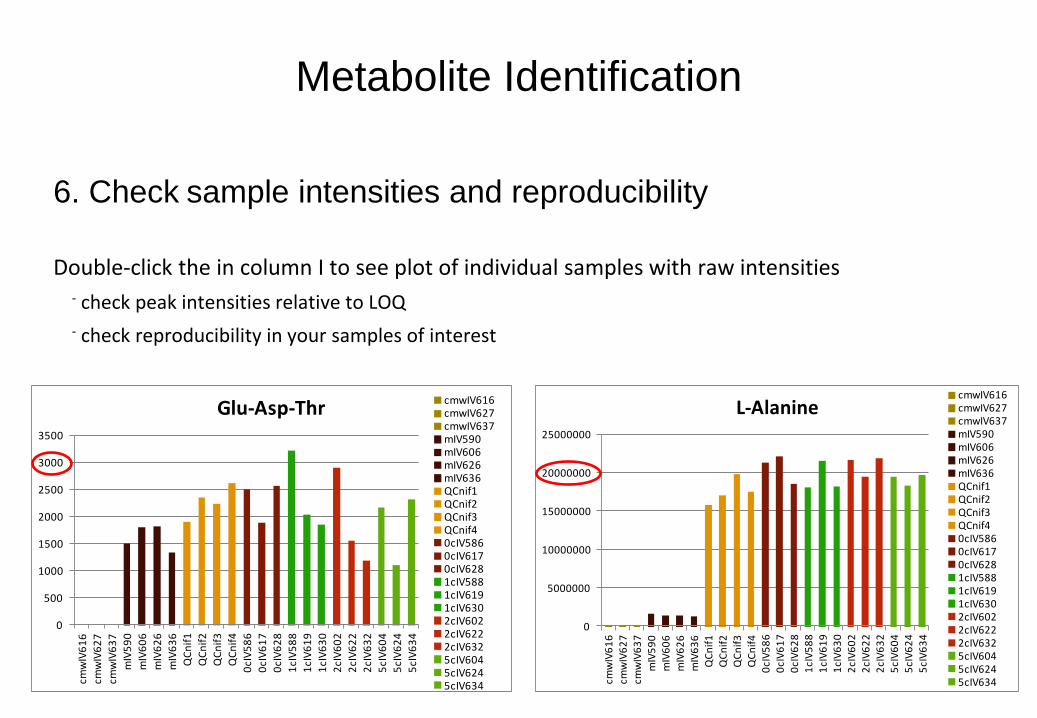
6. Check sample intensities and reproducibility
Double-click the in column I to see plot of individual samples with raw intensities - check peak intensities relative to LOQ
- check reproducibility in your samples of interest
0
500
1000
1500
2000
2500
3000
3500
cmw
IV6
16
cmw
IV6
27
cmw
IV6
37
mIV
59
0
mIV
60
6
mIV
62
6
mIV
63
6
QC
nif
1
QC
nif
2
QC
nif
3
QC
nif
4
0cI
V5
86
0cI
V6
17
0cI
V6
28
1cI
V5
88
1cI
V6
19
1cI
V6
30
2cI
V6
02
2cI
V6
22
2cI
V6
32
5cI
V6
04
5cI
V6
24
5cI
V6
34
Glu-Asp-ThrcmwIV616cmwIV627cmwIV637mIV590mIV606mIV626mIV636QCnif1QCnif2QCnif3QCnif40cIV5860cIV6170cIV6281cIV5881cIV6191cIV6302cIV6022cIV6222cIV6325cIV6045cIV6245cIV634
0
5000000
10000000
15000000
20000000
25000000
cmw
IV6
16
cmw
IV6
27
cmw
IV6
37
mIV
59
0
mIV
60
6
mIV
62
6
mIV
63
6
QC
nif
1
QC
nif
2
QC
nif
3
QC
nif
4
0cI
V5
86
0cI
V6
17
0cI
V6
28
1cI
V5
88
1cI
V6
19
1cI
V6
30
2cI
V6
02
2cI
V6
22
2cI
V6
32
5cI
V6
04
5cI
V6
24
5cI
V6
34
L-AlaninecmwIV616cmwIV627cmwIV637mIV590mIV606mIV626mIV636QCnif1QCnif2QCnif3QCnif40cIV5860cIV6170cIV6281cIV5881cIV6191cIV6302cIV6022cIV6222cIV6325cIV6045cIV6245cIV634

Metabolite Identification
7. Check peak shapes
Hover mouse over the mass in column A to see extracted peaks
- Ideally guassian peaks, some subjective judgement required
Glu-Asp-Thr L-Alanine
Metabolite Identification
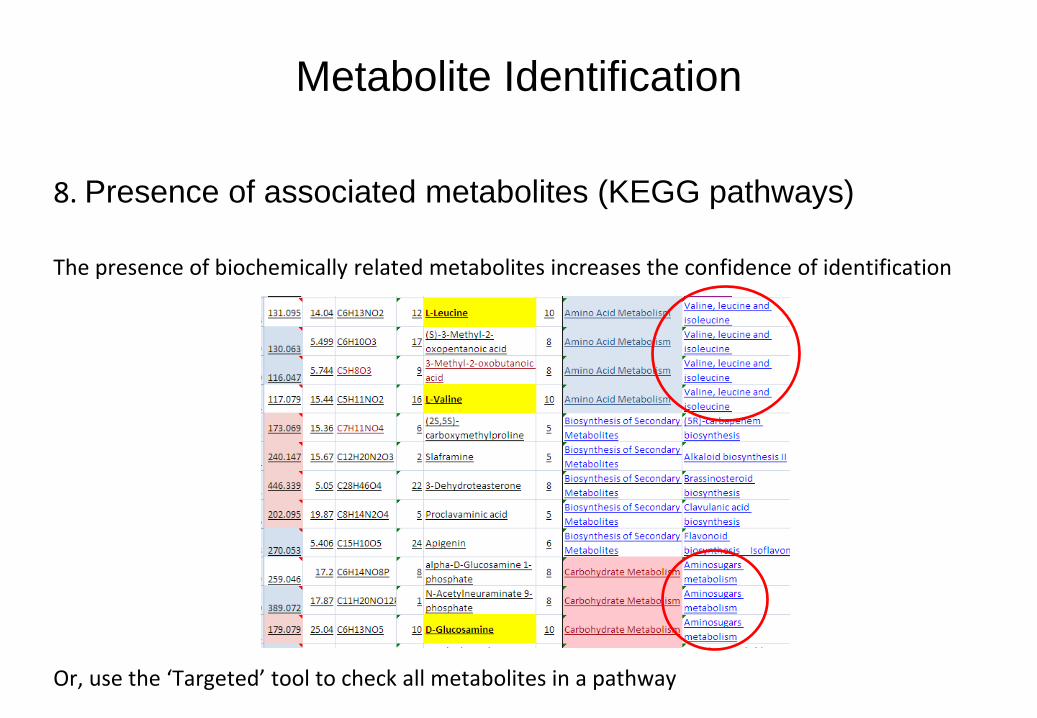
8. Presence of associated metabolites (KEGG pathways)
The presence of biochemically related metabolites increases the confidence of identification
Or, use the ‘Targeted’ tool to check all metabolites in a pathway
Metabolite Identification
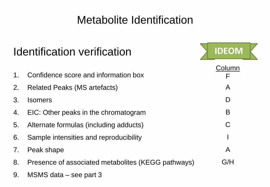
Identification verification
1. Confidence score and information box
2. Related Peaks (MS artefacts)
3. Isomers
4. EIC: Other peaks in the chromatogram
5. Alternate formulas (including adducts)
6. Sample intensities and reproducibility
7. Peak shape
8. Presence of associated metabolites (KEGG pathways)
9. MSMS data – see part 3
Column
F
A
D
B
C
I
A
G/H
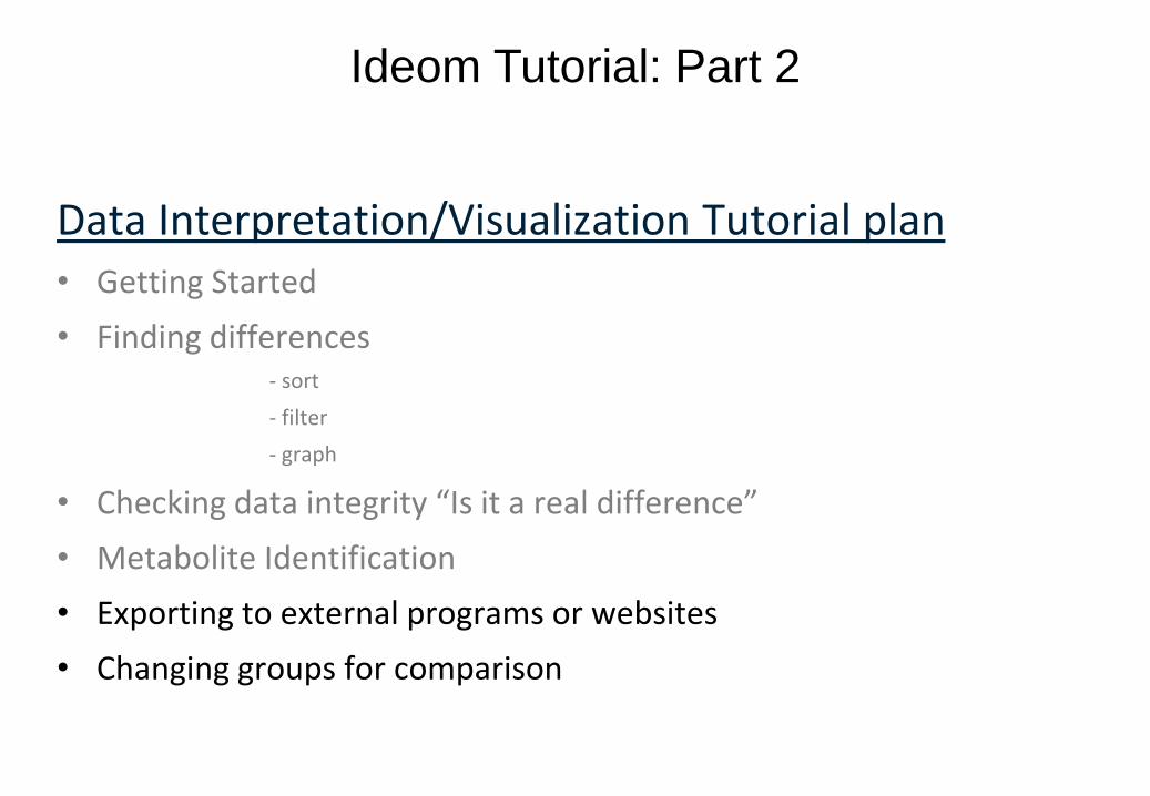
Ideom Tutorial: Part 2
Data Interpretation/Visualization Tutorial plan • Getting Started
• Finding differences - sort
- filter
- graph
• Checking data integrity “Is it a real difference”
• Metabolite Identification
• Exporting to external programs or websites
• Changing groups for comparison

Export data to use external metabolomics applications Click on the “Export for analysis” button to access export options
Export for analysis

Export for analysis
Export data to do multivariate statistics in R
If you are familiar with R you may do additional analyses: The peak intensity data are in “PeakTable”
Samples in rows
Metabolites in columns
Group names in “sampleclasses”
Export for analysis
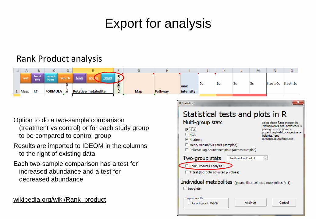
Rank Product analysis
Option to do a two-sample comparison
(treatment vs control) or for each study group
to be compared to control group
Results are imported to IDEOM in the columns
to the right of existing data
Each two-sample comparison has a test for
increased abundance and a test for
decreased abundance
wikipedia.org/wiki/Rank_product
Export for analysis
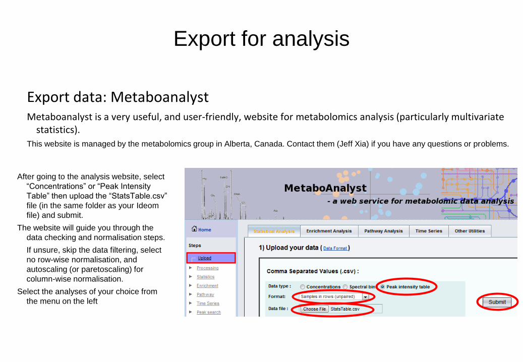
Export data: Metaboanalyst Metaboanalyst is a very useful, and user-friendly, website for metabolomics analysis (particularly multivariate
statistics).
This website is managed by the metabolomics group in Alberta, Canada. Contact them (Jeff Xia) if you have any questions or problems.
After going to the analysis website, select
“Concentrations” or “Peak Intensity
Table” then upload the “StatsTable.csv”
file (in the same folder as your Ideom
file) and submit.
The website will guide you through the
data checking and normalisation steps.
If unsure, skip the data filtering, select
no row-wise normalisation, and
autoscaling (or paretoscaling) for
column-wise normalisation.
Select the analyses of your choice from
the menu on the left
Export for analysis
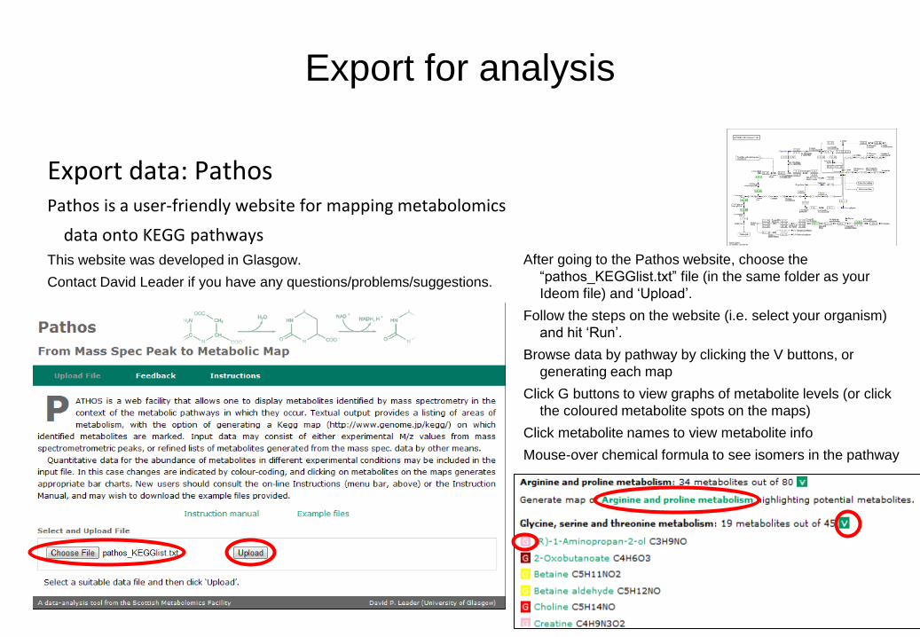
Export data: Pathos Pathos is a user-friendly website for mapping metabolomics
data onto KEGG pathways
This website was developed in Glasgow.
Contact David Leader if you have any questions/problems/suggestions.
After going to the Pathos website, choose the
“pathos_KEGGlist.txt” file (in the same folder as your
Ideom file) and ‘Upload’.
Follow the steps on the website (i.e. select your organism)
and hit ‘Run’.
Browse data by pathway by clicking the V buttons, or
generating each map
Click G buttons to view graphs of metabolite levels (or click
the coloured metabolite spots on the maps)
Click metabolite names to view metabolite info
Mouse-over chemical formula to see isomers in the pathway
Export for analysis
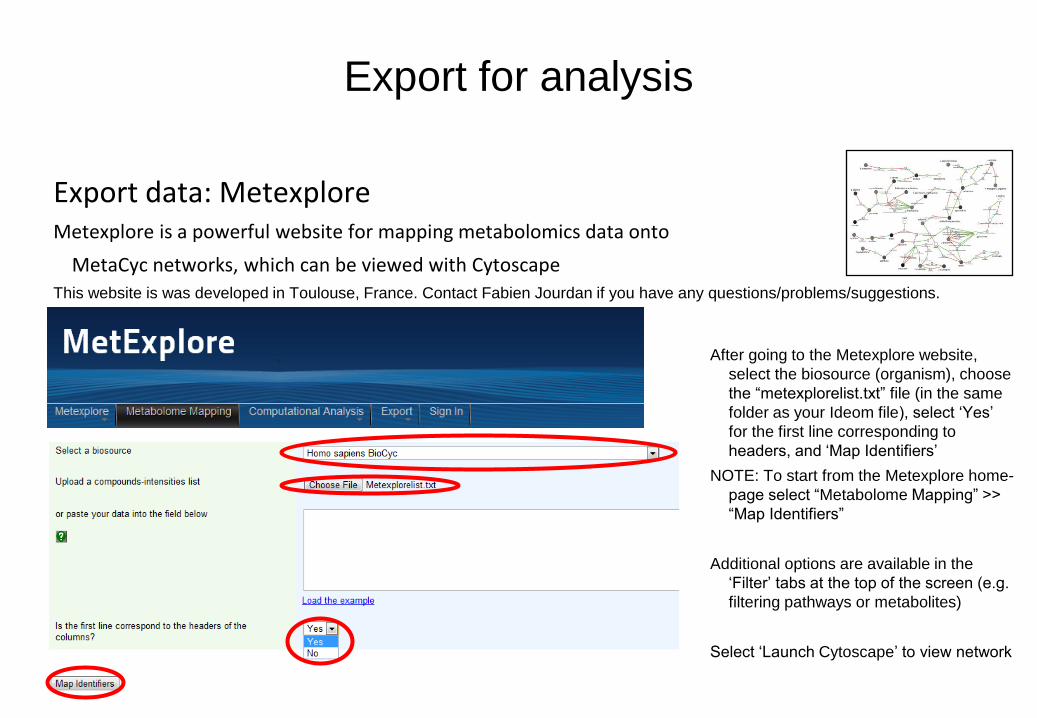
Export data: Metexplore Metexplore is a powerful website for mapping metabolomics data onto
MetaCyc networks, which can be viewed with Cytoscape
This website is was developed in Toulouse, France. Contact Fabien Jourdan if you have any questions/problems/suggestions.
After going to the Metexplore website,
select the biosource (organism), choose
the “metexplorelist.txt” file (in the same
folder as your Ideom file), select ‘Yes’
for the first line corresponding to
headers, and ‘Map Identifiers’
NOTE: To start from the Metexplore home-
page select “Metabolome Mapping” >>
“Map Identifiers”
Additional options are available in the
‘Filter’ tabs at the top of the screen (e.g.
filtering pathways or metabolites)
Select ‘Launch Cytoscape’ to view network

Ideom Tutorial: Part 2
Data Interpretation/Visualization Tutorial plan • Getting Started
• Finding differences - sort
- filter
- graph
• Checking data integrity “Is it a real difference”
• Metabolite Identification
• Exporting to external programs or websites
• Changing groups for comparison
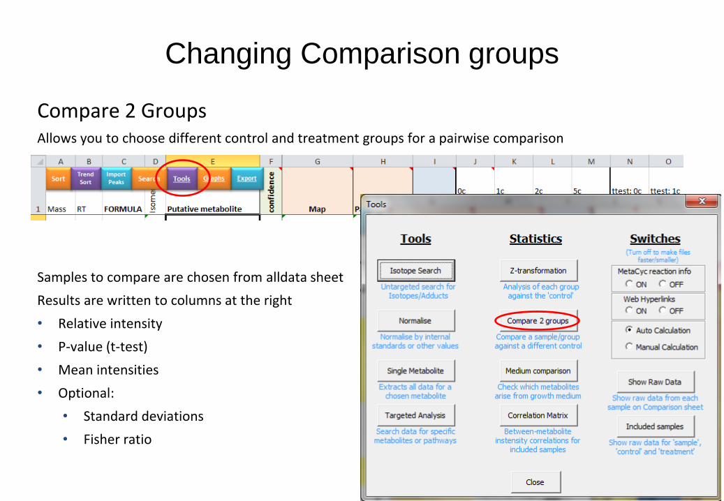
Changing Comparison groups
Compare 2 Groups Allows you to choose different control and treatment groups for a pairwise comparison
Samples to compare are chosen from alldata sheet
Results are written to columns at the right
• Relative intensity
• P-value (t-test)
• Mean intensities
• Optional:
• Standard deviations
• Fisher ratio

Changing Comparison groups
Compare all groups against another control group You may change the control group and re-run the ‘Comparison’ (step 8)
You may also include/exclude other groups from the new ‘Comparison’
1. Go to the ‘Settings’ sheet
2. In column H, change the set-type for each group You should always assign 1 ‘control’ group
NB: you cannot assign more than 1 ‘control’ group
Assign a ‘treatment’ group for two-group comparisons/exports
All other included groups should be assigned as ‘sample’
‘Exclude’ groups that you don’t wish to compare
Click step 8 ‘Compare all sets’ to re-calculate the comparison
sheet based on the new group settings
Caution: if you choose ‘yes’ to including all base peaks it will take much longer

Part 3
Additional features of IDEOM

Additional Features
New and additional IDEOM features
• Further Data Analysis
• Isotope search (for stable-isotope tracing)
• Single metabolite data extraction
• Medium comparison
• Heat maps in IDEOM
• Normalisation
• Fully labelled internal standards
• Signal based (eg. TIC)
• User-defined
• Targeted Analysis
• Standards (3 mixtures)
• Show all charts
• Calibration
• Quantification
• Pathway profile
• Reporting
• Metabolights export
• MSMS annotation
• General IDEOM tools
• Annotate DB
• Import experimental methods
• Import data from old IDEOM file
• General R Scripts
• TIC checker
• Get all chromatograms
• Filter peakml file (create pdf)
• XCMS processing
• Excel functions
• Function formulas
• Mass names
• New applications
• GCMS (low res)

Additional Features
Further Data Analysis
• Isotope search (for stable-isotope tracing)
• Untargeted search for all possible
isotopomers of a list of metabolites
(or unidentified features)
• Supports:
• 13C
• 15N
• 18O
• 2H
• User-defined mass difference
• User manually selects the samples or
groups of samples from mzMatch
sheet (imported peaks)
• Export menu allows targeted isotope
search in raw data through mzMatch.R

Additional Features
Further Data Analysis
• Isotope graphs (for stable-isotope tracing)
• Specific plots to view labelled isotope patterns

Additional Features
Further Data Analysis
• Single metabolite data extraction
• Extracts data for chosen metabolite onto a fresh sheet for you to edit/analyse/graph/etc

Additional Features
Further Data Analysis • Medium Comparison
Mostly the same as the ‘Compare 2 groups’ function
Additional feature annotates if lowest sample intensity is below the highest medium intensity
medium from
medium
not from
medium
Additional Features
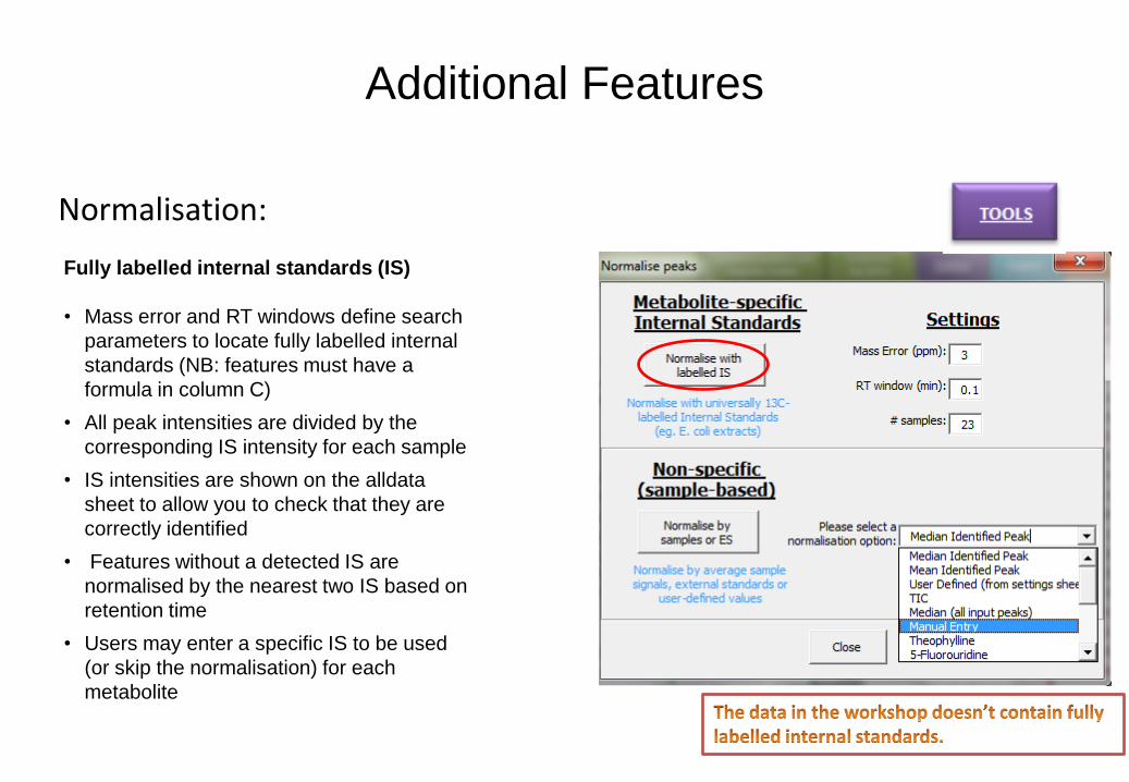
Normalisation:
Fully labelled internal standards (IS)
• Mass error and RT windows define search
parameters to locate fully labelled internal
standards (NB: features must have a
formula in column C)
• All peak intensities are divided by the
corresponding IS intensity for each sample
• IS intensities are shown on the alldata
sheet to allow you to check that they are
correctly identified
• Features without a detected IS are
normalised by the nearest two IS based on
retention time
• Users may enter a specific IS to be used
(or skip the normalisation) for each
metabolite

Additional Features
Normalisation:
Non-specific normalisation
NB: This normalisation is not recommended for
LCMS data except in unavoidable, well-defined
circumstances
• Median/mean identified peak, only uses
metabolites from the identification sheet (i.e. less
bias from noise)
• TIC and median uses all input peaks
• User-defined divides intensities by the values in
column R of the Settings sheet (e.g. enter cell
counts or protein content)
• Manual Entry allows you to enter values for each
sample on the fly
• Further normalisation options are based on the
external standards present in the Settings sheet
(columns U:AD)

Additional Features
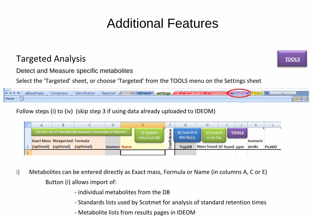
Targeted Analysis
Additional Features
Targeted Analysis Detect and Measure specific metabolites
Select the ‘Targeted’ sheet, or choose ‘Targeted’ from the TOOLS menu on the Settings sheet
Follow steps (i) to (iv) (skip step 3 if using data already uploaded to IDEOM)
i) Metabolites can be entered directly as Exact mass, Formula or Name (in columns A, C or E)
Button (i) allows import of:
- individual metabolites from the DB
- Standards lists used by Scotmet for analysis of standard retention times
- Metabolite lists from results pages in IDEOM
Additional Features
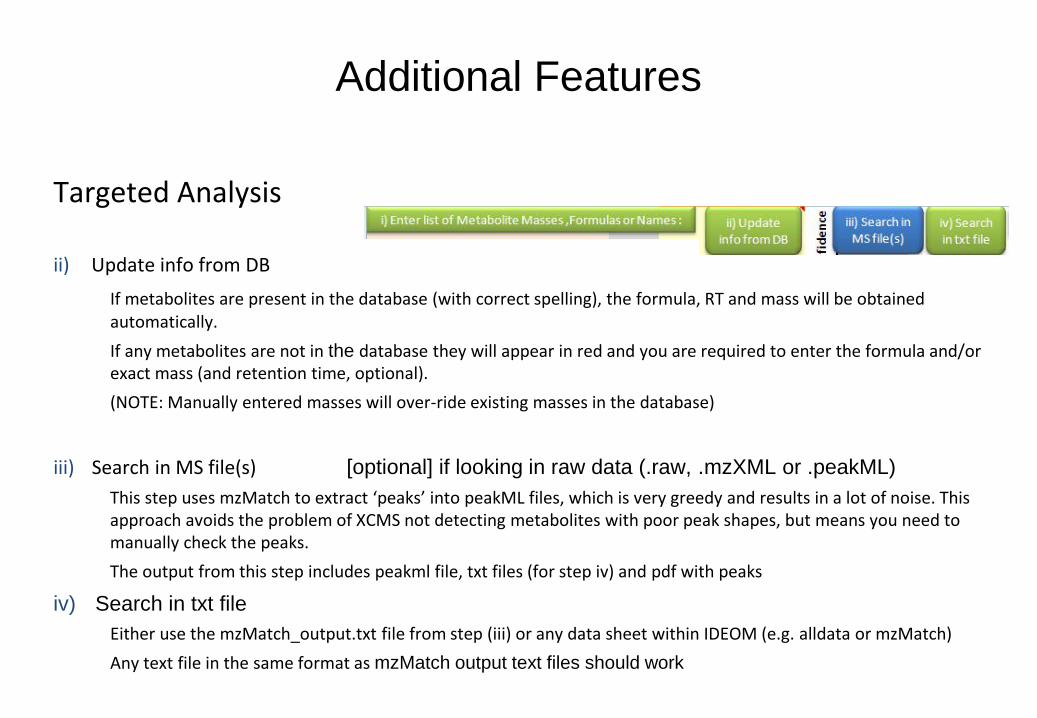
Targeted Analysis
ii) Update info from DB
If metabolites are present in the database (with correct spelling), the formula, RT and mass will be obtained automatically.
If any metabolites are not in the database they will appear in red and you are required to enter the formula and/or exact mass (and retention time, optional).
(NOTE: Manually entered masses will over-ride existing masses in the database)
iii) Search in MS file(s) [optional] if looking in raw data (.raw, .mzXML or .peakML)
This step uses mzMatch to extract ‘peaks’ into peakML files, which is very greedy and results in a lot of noise. This approach avoids the problem of XCMS not detecting metabolites with poor peak shapes, but means you need to manually check the peaks.
The output from this step includes peakml file, txt files (for step iv) and pdf with peaks
iv) Search in txt file
Either use the mzMatch_output.txt file from step (iii) or any data sheet within IDEOM (e.g. alldata or mzMatch)
Any text file in the same format as mzMatch output text files should work
Additional Features
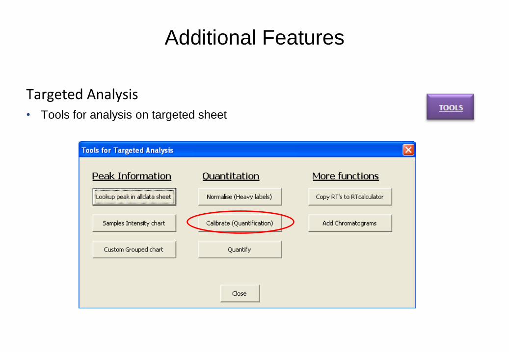
Targeted Analysis • Tools for analysis on targeted sheet

Additional Features
Targeted Analysis
• Calibration
• Generates calibration curves (linear or log-log) and equations for quantification
Quantification (UNDER DEVELOPMENT)
• Quantification of list of targeted metabolites
based on calibration standards

Additional Features
MSMS analysis
• Import and annotate MSMS data
• Convert Raw to mgf file format (with msconvert through R)
• Imports mgf file into fresh page in IDEOM
• Matches precursor ions with peaks in IDEOM data from untargeted analysis
• Lists fragment masses and neutral losses
• Lists likely formula for each fragment and neutral loss (if formula in fragment list)
• Plots MSMS spectra with peak annotation where available
• Links to Massbank and Metfrag for individual verification

Annotate DB
• Adds annotations to the database for new
organisms/studies
• This can also be used as a generic matching
algorithm between IDEOM and other Excel/txt/csv
files
Import IDEOM
• Allows upgrade of data from old IDEOM files (to
allow access to new automated functions).
Enter Study Methods / Sample Details
• Experimental metadata can be stored here
• These sheets are only for recording purposes and
don’t affect Ideom processing.
Additional Features
General IDEOM tools (settings sheet):
Additional Features
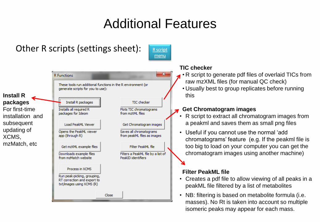
Other R scripts (settings sheet):
TIC checker
• R script to generate pdf files of overlaid TICs from
raw mzXML files (for manual QC check)
• Usually best to group replicates before running
this
Get Chromatogram images
• R script to extract all chromatogram images from
a peakml and saves them as small png files
• Useful if you cannot use the normal ‘add
chromatograms’ feature (e.g. If the peakml file is
too big to load on your computer you can get the
chromatogram images using another machine)
Filter PeakML file
• Creates a pdf file to allow viewing of all peaks in a
peakML file filtered by a list of metabolites
• NB: filtering is based on metabolite formula (i.e.
masses). No Rt is taken into account so multiple
isomeric peaks may appear for each mass.
Install R
packages
For first-time
installation and
subsequent
updating of
XCMS,
mzMatch, etc

Additional Features
Excel functions
‘User-Defined Formulas’ can be used in any
Excel cell
fx =ExactMass(formula, Clabels,Nlabels,Olabels,Dlabels)
• Calculates the exact mass from a formula
• Supports heavy isotope labelled metabolites
• Only common atoms supported: C,H,N,O,S,P,Cl,F,I,Br,Se
fx =ppmcalc(mass,theoreticalmass, formula)
• Calculates the mass difference (in ppm) between a given
mass and a theoretical formula or mass
fx =formulaMATCH(mass, ppm, masslist, formulalist)
• Finds a matching formula in a database of ascending
masses (e.g. the DB sheet).
• If two masses either side of the search mass are within
the allowable ppm error the answer is italicised
fx =Formulavalid(formula)
• Checks the validity of a proposed chemical formula
against 5 of Kind & Fiehn's 7 golden rules
fx =IsotopeAbundance(formula, atom)
• Calculates the theoretical natural isotope
abundance of a specified atom in a given formula
(relative to basepeak)
fx =Pos(pH, cation, pka1,pka2,pka3,...) & Neg
• Calculates the average number of charges on a
molecule at a given pH
fx =FormulaReactor(formula1,formula2,formulaloss)
• Adds the atoms of two formulas to give the formula
(e.g. for adduct prediction)
• Also allow subtraction of one formula from another
(e.g. for fragment prediction)
fx =proton & Naadduct & Kadduct & Cladduct
• Returns the exact mass (these are Excel names)

Additional Features
GCMS processing (low resolution)
• Automated identification of metabolites in standards
database
• Identified by quant ion and Rt
• Spectral match score provided (but not essential for
ID)
• Qual ions #1 & #2 relative intensity provided (but not
essential for ID)
• Links from individual metabolites (spectra) to Golm
metabolite DB for identification of unknowns

Acknowledgements
Andris Jankevics
Unni Chokkathukalam
Karl Burgess
Rainer Brietling & team
Mike Barrett & team
Dave Watson & team
(Gavin Blackburn, Alex Zhang, Leon Zheng)