Stepper motor vibrations

Introduction In this paper I am dealing with stepper motors from the point of an advanced hobbyist. It is supposed that the reader already has some understanding about what a stepper motors is. I promise that the math needed to understand ideas discussed in this paper is going to be undemanding. Stepper motors are popular among hobbyists as a cheap way to build positioning systems. A stepper motor position (that is, its rotor angle) can be controller cheaply and accurately. Other inexpensive electric motor types, like DC motors or asynchronous AC motors, might work for speed control or torque control, but suck if you try to use them for position control. On the other hand, servo motor systems can position even quicker and more accurate than stepper motors, but are also more expensive. Comparison between basic motor types Before we concentrate on stepper motors, let me make a short comparison between most common electric motor types to help us understand better what a stepper motor is: DC motors and universal motors These are 'soft voltage-to-speed' motors - depending on the voltage you feed to them, these motors will achieve some final speed when non-loaded. Higher the voltage, higher the final non-loaded speed, and the dependence is linear. At its non-loaded final speed, the motor consumes very little power and doesn't draw much current. If you then put some load to the motor, the speed will somewhat decrease, the current will increase and the power will be consumed. The torque generated by the motor (that is, the load you put to it) is proportional to the speed decrease. Because the speed decreases with increasing load, I call DC motors 'soft voltage-to-speed' motors. Of course, DC motors can act as generators – if you turn its shaft faster then its non-loaded-speed, the motor will start generating power, and you will feel this because faster you turn the shaft, more torque it will require. DC motors are also 'current-to-torque' motors – if you feed constant current to them, these motors will provide constant torque. If unloaded and feed with current, the DC motor will accelerate to ‘infinite’ speed (sure, there are loses that will limit this ‘infinite’ speed). DC motors can provide soft speed control (by feeding voltage to them), and torque control (by feeding current to them). They cannot provide position control unless you used some external position sensors and some loop-back method.

AC asynchronous motors These are ‘soft frequency-to-speed' motors with charming simplicity and reliability. You must feed AC voltage to them. The non-loaded motor will achieve a speed that directly depends on the frequency of the AC voltage. When you then put the load to the motor, its speed will somewhat decrease. This difference between the non-load speed (synchronous speed) and a loaded speed is called 'slip'. How much the speed will decrease with the increased load, depends on the current amplitude that motor is consuming (and the current amplitude, in turn, depends on the AC voltage amplitude you feed to the motor) – higher the current, the motor will resist to the speed decrease harder. Note that as the AC frequency increases, you also need to increase the voltage amplitude to keep the load-to-slip ratio about the same. Keeping frequency and voltage amplitude proportional is actually the way to keep the motor current amplitude constant… Unfortunately, the load-to-slip ratio (that is, the torque-to-slip ratio) of an asynchronous motor is not represented by a simple proportionality law – if the slip increases above some level, the torque will not rise any more, but will start decreasing, and the motor will quickly stall. AC asynchronous motors will act as generators if you turn their shaft faster than is their synchronous speed. AC asynchronous motors can provide soft speed control when feed with AC voltage of regulated frequency and amplitude. This requires an inverter circuit and a quite smart inverter control. If the inverter is smart enough, it can even provide sensorless torque control. However for position control you will need some external position sensors. AC synchronous motors These are 'hard frequency-to-speed' motors. Their speed depends only on to the frequency of the AC voltage (or current) that you feed to them. When you put some load to them their speed will not decrease, but their phase will retreat somewhat. Once you put too much load, the motor will jump out of synchronism and will suddenly stall (or become erratic). How much load you can put before it happens, generally depends on the AC voltage amplitude you feed to the motor (and on motor characteristics, of course). AC synchronous motors are the class of motors that is most interesting to us now because stepper motors (and most servo motors, by the way) are also members of this class. AC synchronous motors can be small motors used in watches, or large gigawatt units used as generators in electric power plants. Some have only two poles, while others, like stepper motors, might have hundred poles. What makes AC synchronous motors unique is the fact that this motor will not creep if you put some load to it – it will resist any continuous creeping and will always remain in a more-or-less the same phase as is the voltage that is feed to it. Thanks to this, it is possible to know the position of its rotor without having any position sensor (as long as you know its initial position and you are sure the load on the motor will never become too large to force the motor out of synchronism). Therefore, AC synchronous motors can provide position control without external position sensor.

Comparison between servo motors and stepper motors Servo motors (here we talk about AC servo motors with permanent magnet) and stepper motors (here we talk about stepper motors with permanent magnet) are the same class of motors and are thus quite similar. From construction point of view, the main difference is that a typical servo motor has low number of poles (P=2 to P=8), while a typical stepper motor has large number of poles (say, P=25 to P=100). An additional difference, but not very important, is that servo motors are most often built as three-phase motors (have three sets of windings) while stepper motors are usually built with two sets of windings. These two separate windings in a typical stepper motor allow for simpler motor driving than it is the case with three interconnected (star or delta) windings in a typical servo motor. When a torque is applied to either servo motor or stepper motor, its shaft will turn for some angle (but will not keep moving any further). At the maximum torque a motor can take, its shaft will move for about 180/P degrees in one direction. Any higher torque would kick the motor out of synchronism. For a positioning system it is undesirable to have large shaft movements when applied torque varies because this makes positioning inaccurate. As you can suspect, because servo motors have smaller number of poles ‘P’, a servo motor will keep its position less accurate than a stepper motor of the same rated torque. As a result, servo motors always have external position sensor (a rotary encoder or a resolver) and use a closed-loop control to achieve great positional accuracy. This makes servo motor systems more complex and more expensive. Stepper motors, on the other hand, are intentionally built with large number of poles so that they can achieve acceptable positional accuracy even without closed-loop control and external position sensors. Unfortunately, large number of poles makes them low-speed and low-power (for the equal size) solutions when compared to servo motors. One will typically use servo motors in demanding applications, while stepper motors are reserved for cheap, undemanding (low speed, low power, medium precision) applications and for, of course, hobbyist usage. One typically buys the servo motor driver, while stepper motor drivers are more often built from scratch. Although stepper motors can be used for position control in the open-loop mode, a hobbyist will quickly learn that deploying stepper motor drivers of simplest design would severely limit motor speed and may introduce nasty vibrations. More elaborated stepper motor drivers are needed to use the stepper motor to its fullest. Unfortunately, it is questionable if a complex stepper motor driver makes sense because many times it might just make more sense to buy a servo motor system instead. Making an elaborated stepper motor driver at home is fun, but the economic value of such endeavor is questionable.

Stepper motor basics Consider an electric motor as depicted on the picture below:

This motor has: stator (the hatched outside part), rotor (the gray central part), and two windings (red and green). Note that the rotor is actually a permanent magnet and has its south and north pole. Also note that, to make a symmetrical motor, both the green winding and the red windings are split into two equal parts (with the rotor in between). Windings, red and green, together with stator iron create electromagnets. The red winding creates a vertical electromagnet, while the green winding creates a horizontal electromagnet. As you can see on the picture below, magnetic flux lines (thin blue lines) from these two electromagnets runs through the rotor and close over the stator.

In this example we used some DC voltage on the green winding, while we keep the green winding unconnected. This creates the horizontal electromagnetic field across the rotor, and because the rotor is also a permanent magnet, the rotor will rotate and align itself with the horizontal magnetic field. Depending on how we connect the DC voltage to windings, we can control the position of the rotor, as shown on the following pictures.

But as you probably know already, we can do much more than the above. Instead of feeding DC voltages to one winding at a time, we can feed voltages to both windings simultaneously. The resulting magnetic field will be the vector sum of fields created by horizontal and vertical windings. Obviously then, if we want to generate the magnetic field at the angle of , we just need to generate following voltages at x and y windings.

Where vx and vy are voltages to be feed to the x (green) and y (red) windings. V0 is the ‘voltage amplitude’ and higher this value is, the stronger is the magnetic field we are generating inside the motor. If, for example, we feed AC voltages (described with two simple equations below) to our motor, the rotor should keep rotating smoothly and with constant speed (the rotational speed is , and its unit is radians per second).

In practice, however, the rotation will not be as smooth as we desire – considerable vibrations can be created especially when a stepper motor is driven by a square wave voltage. The reason I am writing this paper is to address these vibration problems. In practice, because of simplicity and other reasons, a stepper motor is often feed with square voltages instead of sine-wave voltages. However in this paper, unless otherwise noted, we are assuming sine-wave feeding to the motor. We learned now how we can orientate the stator magnetic field inside the motor to any desirable angle. The rotor orientation will then follow the stator magnetic field orientation pretty closely supposing that the rotor is not loaded. The AC voltage applied to the motor and the rotor magnetic field orientation will only be in the same phase if the AC voltage that is feed to motor has low frequency. But when a high-frequency AC voltage is applied to the motor in order to achieve high rotational speed, the current through motor windings will start getting late in phase compared to the voltage. Therefore, because the magnetic field is generated by the current, the magnetic field will also move behind the voltage phase (up to pi/2 radians at very high frequencies). This is normally not a big problem, but should be noted.

I also said that stepper motors usually have large number of poles, but our example motor at pictures above only has two poles. There is a charming trick to achieve large number of poles without introducing much complexity to the motor. At the picture below a 20-pole motor is depicted – notice that the rotor permanent magnet now has multiple poles and that stator now has some dents.

Further in this paper we won’t much discuss the number of poles (nor the number of steps per revolution) that a stepper motor has. Instead we are going to do math as if we are dealing with a 2-pole stepper motor (that is, a 4-step stepper motor). In this paper when we say that the rotor rotates for 2*pi radians, it actually means that the rotor rotated for one full step cycle (4 steps) – how many steps does it takes for the rotor to actually finish the full rotation, we don’t care. In the theoretical discussion that follows, results are relevant even if we are considering two-pole stepper motor – all we have to take care is to sufficiently reduce the rotor moment of inertia. (One full step cycle at the 200-step stepper motor will only produce 1/50-th rotor movement compared to a 4-step stepper motor. From mathematical point of view, a 200-step stepper motor is the same as 4-step stepper motor with rotor that has 50 times smaller moment of inertia – at least in the first approximation). One more point before I finish this chapter – if you slowly rotate the rotor of an unconnected stepper motor with your hand, you will feel ‘dents’. This is normal and is typical for a stepper motors with permanent magnets. These dents are felt because the rotor permanent magnet gets aligned with stator dents. In some cases this is desirable characteristics of a stepper motor as it allows the motor to keep its position even when not connected to a power supply (supposing that the holding torque needed is really small). In other cases this is undesirable because, as other people say, these dents generate some additional drag at high rotational speeds (this claim would deserve some mathematical background check, but in this paper I am not doing it). Stepper motor model In this chapter I am going to present a simplified model of a stepper motor. Hopefully we can better understand what is happening inside the stepper motor when we have the model at our hand. Most values present in my stepper motor model (voltages, currents, magnetic fields, rotor position…) are represented by two-dimensional vectors. In reality, for example, there exist x and y current components, but in the represented model the current is a single vector that has its angle and its length (and you can always disassemble it into x and y

components). In realty, you will feed x and y voltages to the motor, but in the model you feed voltage vector ‘u’ to the motor.

Motor’s windings (resistance ‘Rtot’ and inductivity ‘L’) are modeled using the ‘1/L’ gain in front of an integrator, the integrator itself, and using the ‘Rtot’ gain in the short feedback branch. The idea is that windings are composed of an ideal inductivity and a resistance in series. The current that flows through the resistance generates some voltage drop (=I*Rtot) and thus only the remaining voltage ‘uL’ drives the current through the ideal inductivity ‘L’. The current ‘i’ that flows through windings generates stator magnetic field vector ‘B’. To get the torque that is generated on the rotor, the stator magnetic field vector ‘B’ is multiplied (by vector product) with the rotor magnetic moment vector ‘m’. The produced torque ‘T’ is not a vector, but just a scalar value as we are working in the 2D space. Note also that the vector product element is a non-linear element. The torque generated by the magnetic field ‘T’ accelerates/decelerates the rotor – integration gives rotational speed ‘’, and further integration gives the rotor angular position ‘’(all scalars). The rotor angular position ‘’ is then transformed into the angular position vector ‘’ (the ‘’ vector has the length equal to one) and this transformation is represented by the ‘sin/cos’ block. The angular position vector is multiplied with the constant ‘IR*S’ to get the rotor magnetic moment vector ‘m’. The most important thing to understand from the above model is that the rotating rotor, being a permanent magnet, also generates some voltage in the motor windings. This voltage is called back-emf (back electromotive force) and in the model it is labeled as the ‘emf’ vector… The rotor magnetic moment vector ‘m’ generates the magnetic flux through motor windings that is represented by the vector ‘’. The changing of the magnetic flux vector ‘’ (that is, the derivation of ‘’) generates the voltage (the back-emf) in every turn of winding wire. The back-emf generally opposes to the input voltage – that is why in the model the ‘emf’ is subtracted from the input voltage vector.

For those of you that finished the school some time ago, just a reminder: When a vector signal gets integrated, the resulting vector signal is retarded in phase for pi/2. When a vector signal gets differentiated, the resulting vector signal is advanced in phase for pi/2. Of course, amplitudes also change – when integrated the amplitude gets divided by the signal frequency, and when differentiated the amplitude gets multiplied by the signal frequency. Sometimes we feed current to the stepper motor instead of the voltage. This simplifies our model greatly. Here is the model of a stepper motor that is current-fed (as you can see, nothing much is left):

When you feed the current to the motor, neither the winding resistance nor winding inductance has any effect. The same can be said about the back-emf. These things still exist and the current source that feeds the motor will feel them all, but as the power supply is capable (by definition) of forcing the needed current despite all this back-voltage that comes from the motor, we were able to drop these nasty things out of the model. The back-EMF Only someone very naive would not consider the back-emf created by the motor when the motor is running. The back-emf is nature’s way to keep things in order and is unavoidable in all electric motors. The back-emf spoils any romantic thought you had about electric motors when you were a child… In this chapter we are dealing with the back-emf in details, and this is the most intensive chapter in this whole paper. Let us make an experiment. Take a stepper motor; do not connect its winding wires to any voltage source – only connect voltmeters to winding wires. Set voltmeters to AC range.

Having this setup, we are now going to rotate the rotor of the stepper motor by hand (or some other mean). First we will rotate it slowly, and then faster and faster. Immediately we will see that voltmeters do show some voltage. Faster we rotate, higher voltage is generated by the motor – the generated voltage is directly proportional to the rotation speed. This voltage generated by rotor rotation is called the back-emf (the back-generated-electromotive-force). This back-emf voltage is the reason why the motor can be used as a generator. The back-emf is generated because the rotor permanent magnet moves (rotates) and this creates changeable magnetic flux through motor windings. The created voltage in the winding is given as

where ‘’ is the magnetic flux through the winding, and ‘N’ is the number of wire turns in the winding. The important thing here is to understand that the back-emf is generated always when the rotor rotates. It is generated as well when we turn the rotor by hand, as when the rotor is turned by supplied voltage. Of course, when we supply the voltage to the motor we will not be able to measure the back-emf as easily as in the above experiment because the supplied voltage and the current that runs through windings will interfere with our measurements, but the back-emf is still present. Just for exercise, let us examine our above experiment by using our stepper motor model. When I say ‘leave the wires unconnected’ it means that we must put some infinite resistance in serial to windings – in our model this is the same as if we increase ‘Rtot’ to infinite. There is no current through windings, no magnetic field generated by windings, no torque generated by magnetic field. In addition we are providing rotational speed directly by our hand… thus, our model degenerates into:

This is a very simple, straightforward model without loops. The thing to note is that the amplitude of the generated back-emf signal is proportional to the rotor speed ‘E’ (because the differentiator that differentiates the rotor magnetic flux vector will produce a vector whose amplitude (length) linearly increases with signal’s frequency).

In the second, much more complex experiment, we are going to short-circuit motor windings and then we will turn the rotor by hand.

First thing that you will notice is that now it is much harder to turn the rotor. Some torque (drag) is generated by the motor that tries to resist you as you are revolving the rotor. The reason is because the back-emf voltage now generates currents in the windings. It happens that those currents are arranged in the way that creates an opposing torque in the motor so that you feel it as a drag. In fact, if you put ammeters (set to AC range) into the circuit, you could measure these currents generated by the back-emf. Because, as we said, the back-emf amplitude rises linearly with the rotation speed (frequency) we can expect that the generated current will also rise with the increasing rotation speed. However because windings have both, resistance and inductance, we can expect that the current will only rise to some level and will then remain constant despite the further increase in rotation speed. You see, at very high frequencies it is the winding inductance that limits the current and an inductance doesn’t like to pass high frequency currents – so current amplitude remains constant. This indeed is what is happening. If you put some torque-meter between your hand and motor’s shaft, you will be able to measure the torque that is needed to rotate the rotor at various rotation speeds. Therefore you will be able to measure the torque (drag) generated by the back-emf. As rotation speed increases, the torque would also increase… but only up to some point. After that, surprisingly, any further speed increase reduces the needed torque… Hell! What is happening!?

The rough sketch above shows how the back-emf, the current, and the torque change with increasing rotor rotation speed in our experiment. To understand the reason why the torque starts decreasing toward zero at high rotational speeds, we will use our stepper motor model.

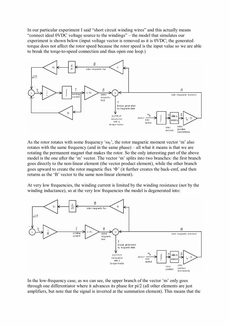
In our particular experiment I said “short circuit winding wires” and this actually means “connect ideal 0VDC voltage source to the windings” – the model that simulates our experiment is shown below (input voltage vector is removed as it is 0VDC; the generated torque does not affect the rotor speed because the rotor speed is the input value so we are able to break the torqe-to-speed connection and thus open one loop.)

As the rotor rotates with some frequency ‘E’, the rotor magnetic moment vector ‘m’ also rotates with the same frequency (and in the same phase) – all what it means is that we are rotating the permanent magnet that makes the rotor. So the only interesting part of the above model is the one after the ‘m’ vector. The vector ‘m’ splits into two branches: the first branch goes directly to the non-linear element (the vector product element), while the other branch goes upward to create the rotor magnetic flux ‘’ (it further creates the back-emf, and then returns as the ‘B’ vector to the same non-linear element). At very low frequencies, the winding current is limited by the winding resistance (not by the winding inductance), so at the very low frequencies the model is degenerated into:

In the low-frequency case, as we can see, the upper branch of the vector ‘m’ only goes through one differentiator where it advances its phase for pi/2 (all other elements are just amplifiers, but note that the signal is inverted at the summation element). This means that the

‘B’ field vector that enters the non-linear element is at pi/2 phase difference compared to the ‘m’ vector that enters the same non-liner element from the other side. The non-linear element produces torque by the formula:

Note also that the ‘B’ vector amplitude is proportional to ‘emf’ vector amplitude which is in turn proportional to the rotational speed (as we said earlier). Thus we can say that at low frequencies the torque rises proportionally with the increasing rotation speed.

At very high frequencies, the current is limited by the winding inductance, while the resistance does not have much effect. So, we can drop the winding resistance from our motor model:

Obviously at high frequencies, the ‘m’ vector that goes to the upper branch first meets one differentiator (advances signal phase for pi/2) and after that one integrator (hinders signal phase for pi/2) on its path to the non-liner element. As a result, the ‘m’ vector that enters the non-linear element from the right, and the ‘B’ vector that enters the non-linear element from the left are in exact anti-phase (that is, the phase difference is pi). As a result, the non-linear element produces zero torque.

We can conclude: At very low frequencies the torque generated by the back-emf rises proportionally as the frequency rises; somewhere at middle frequencies the torque reaches its peak value; as the frequency rises further, the torque slowly drops back toward zero. The reason why the torque starts decreasing is not because the back-emf decreases (the back-emf

actually continues to rise), nor is it because the current decreases (the current stays at some constant level), but because the phase difference between the current vector ‘i’ (and thus also the ‘B’ vector) and the rotor position vector ‘’ (and thus also the ‘m’ vector) approaches toward pi… At the picture below you can see the rotating vectors ‘m’ and ‘B’ in the motor at various frequencies. Note that B vectors changes its phase in comparison to ‘m’, and also increases in length as the frequency rises.

I spent lot of time explaining why the back-emf generated torque reduces at high speed because I hope that this understanding will be useful to us later. For those of you who are familiar with a typical torque curve shape of an asynchronous AC motor, the curve shape of a stepper motor is not a complete surprise. In an asynchronous AC motor the torque curve also tends toward zero as the slip becomes very large (and for the very similar reason). But I am still far from finishing this chapter. I want to compute the frequency at which this back-emf generated torque (drag) has its maximum. More formal math analysis follows… I will consider only the relevant part of our stepper motor model…

First, I will check how ‘B’ vector depends on ‘m’ vector… To make this simpler, I will join several amplifiers together. More importantly, I will only examine one (y) component of ‘m’ and ‘B’ vectors to make the computation using scalars instead of using vectors. (I can always suppose that the x vector component behaves the same as the y component, only it is phase is advanced by pi/2).

I am going solve the system equation by switching into the Laplace domain and then by doing some math gymnastics.

In the solution above we removed the exponential-decay part because we are not interested in a transient solution. We can now immediately write the x component of the ‘B’ vector because we know that it looks just like the y component, only with the phase difference of pi/2. Now we have following solutions for the ‘B’ vector in comparison to the ‘m’ vector:

The above two vectors ‘m’ and ‘B’ are rotating with the frequency ‘’. However we are not interested in how these vectors rotate – we are mostly interested in their lengths and the phase difference between them. Both of these two values, the vector length and the phase difference,

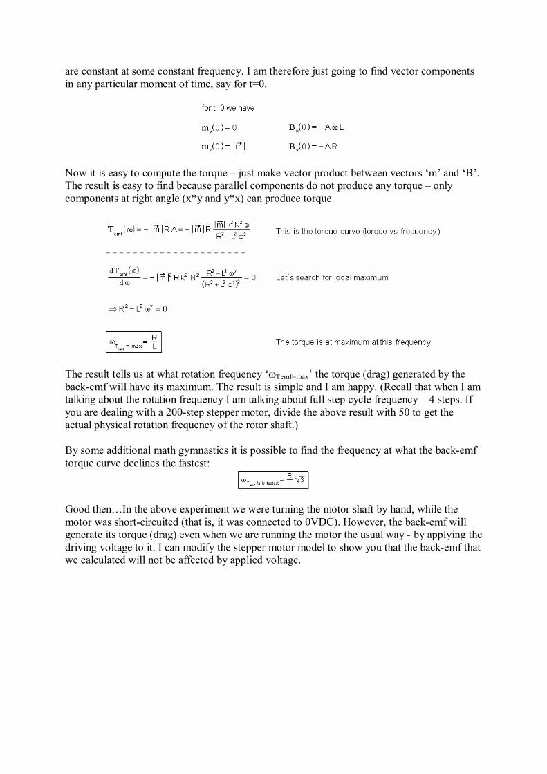
are constant at some constant frequency. I am therefore just going to find vector components in any particular moment of time, say for t=0.

Now it is easy to compute the torque – just make vector product between vectors ‘m’ and ‘B’. The result is easy to find because parallel components do not produce any torque – only components at right angle (x*y and y*x) can produce torque.

The result tells us at what rotation frequency ‘Temf=max’ the torque (drag) generated by the back-emf will have its maximum. The result is simple and I am happy. (Recall that when I am talking about the rotation frequency I am talking about full step cycle frequency – 4 steps. If you are dealing with a 200-step stepper motor, divide the above result with 50 to get the actual physical rotation frequency of the rotor shaft.) By some additional math gymnastics it is possible to find the frequency at what the back-emf torque curve declines the fastest:

Good then…In the above experiment we were turning the motor shaft by hand, while the motor was short-circuited (that is, it was connected to 0VDC). However, the back-emf will generate its torque (drag) even when we are running the motor the usual way - by applying the driving voltage to it. I can modify the stepper motor model to show you that the back-emf that we calculated will not be affected by applied voltage.

This is the same motor model, only now the input voltage vector ‘u’ path and the ‘emf’ vector path are separated to show that the back-emf generated torque ‘Temf’ only depends on the rotor rotation speed. The torques generated by the input voltage ‘Tv’ and by the back-emf ‘Temf’, both being simple scalar values, are then summed. Also note that in the above diagram I added the ‘Rv’ resistance in series to winding resistance making the total resistance Rtot=R+Rv. The ‘Rv’ resistance is usually the internal resistance of the voltage source used to drive the mtoro (because the voltage source we might be dealing with is not necessarily an ideal voltage source). We already calculated how the back-emf torque, Temf(), depends on the frequency. We also know at what frequency the torque has its maximum; we can now easily compute the maximal back-emf generated torque

Obviously we cannot change the ‘Temf max’ for a given stepper motor (neither ‘mA’, ‘k’, ‘N’ nor ‘L’ are configurable). We can however change the frequency at which the maximum torque (drag) is generated by changing the ‘Rtot‘ – more precisely, we can change the ‘Rv’ component of the ‘Rtot’.

As you can see, if we want to maximize the back-emf generated torque at some particular frequency ‘’, we can do this, within some limitations, by adjusting the ‘Rv’ resistance according to the above formula. Feeding a stepper motor You can feed either current or voltage to a stepper motor. You can also choose if you will feed sine wave, square wave or some other waveform to a stepper motor. Feeding current is simpler from theoretical point of view as you don’t have to take care about the back-emf generated by the motor. You directly feed the current to motor windings and any back-emf that might come from the motor is not able to change this current. Unfortunately, in practice, feeding current is not easily implemented, especially if you want your motor to run at high speeds. To feed current, you need to use some current source, and making a current source might not be a trivial task (If you build a simple current source without a feedback loop, it will make a lot of heat and waste a lot of energy. Or you can make more complex switching-mode current source that uses feedback loop to keep the current at the commanded level, but this is somewhat complex (although there are chips today that will do this) and you might need high voltages once you run your motor into high revs). Feeding current to the motor will wipe out stepper motor instabilities at high speeds. But, as I said, this comes with a price because at high speeds you will need highly capable current source to maintain the desired current at those high revs where the high level of back-emf is present. Feeding current, as I define it, does not only mean that you have to keep the current amplitude through the motor windings at desired level. It means that you also have to keep the current phase at the desired value. As a result, your current source will need to provide more and more voltage to the motor windings as the speed rises to counteract the back-emf. When you feed current, you will normally choose to keep the current amplitude constant across the whole speed range. This way the available torque from the motor is going to be approximately constant across the whole speed range. This also means that the available mechanical power will rise linearly with the speed (power=torque x rotational speed). In practice, at high revs more loses are expected by eddy currents and magnetization hysteresis. Also remember that motor winding insulation can only withstand so much voltage and at high revs your current source will provide a lot of it. Voltage feeding is another beast. In this case the motor will throw at you all kind of its back-emf garbage making theory more complex. But in practice, building a voltage source is easier than building a current source. When you feed voltage to the motor you must know that at low motor speeds (including the case when the motor is just held standing still) you need to reduce the voltage or otherwise the current might quickly rise to destructive levels. As the rotation speed increases, you will be increasing the voltage - this will, supposing that we run the motor still in the relatively low speed range, keep the current approximately constant and thus maintain the torque. Once you reach some medium revs, you will stop increasing the voltage amplitude any further as you continue to increase the frequency because you will reach the maximum voltage level

(it is either limited by your voltage source abilities or limited by your motor insulation abilities). Somewhere here your motor will run into an unstable region that we will discuss later in this paper.

The two cases of voltage feeding are displayed in diagrams above. In the first case the voltage amplitude is kept constant at all frequencies and this causes very high currents at low speeds (overheating). To compensate for this in the second case the voltage that we feed to the motor is reduced at low speeds so that the current is always kept at or below the motor nominal level. At very high frequencies the current is driven by the back-emf, and that is why the current changes its phase and why it reaches a constant level (recall that we already made that conclusion in the back-emf chapter). In the case that the frequency is high enough so that the back-emf amplitude is much larger than the feed voltage amplitude, we can see from the stepper motor model that the current will be constant and will only depend on physical motor characteristics (note that at very high frequency the back-emf and the feed voltage are in almost complete anti-phase, so it is really easy to compute):

The more interesting part is that the current curve has its minimum at some frequency. I find it difficult to analytically compute the frequency at which the current has its minimum (note that the current does not have to reach the zero - certainly not if the motor is under load). After that minimum, with increasing frequency, the current changes its phase for pi, and continues to the already explained stationary level. The reason why the current has its minimum is because at this frequency the back-emf voltage mostly cancels out the feed voltage (that is the back-emf amplitude is nearly equal to the feed voltage amplitude, while both vectors are in near anti-phase). The minimum current level, however, happens near (but not necessarily exactly at) the point where the back-emf amplitude is equal to the feed voltage amplitude. Therefore we could at least approximately compute the frequency where it happens. From our stepper motor model, we see that the ‘emf’ amplitude can be written as:

We see that the current will have its minimum on the frequency that linearly depends on the feed voltage amplitude. Larger the voltage amplitude we feed to the motor, later the current minimum will happen. This is all expected… The one thing to remember is that the frequency at which the current curve reaches its minimum is not related to the frequency at which the back-emf generated torque curve reaches its maximum (recall: emf max=Rtot/L). In most cases the frequency at which the minimum current is reached will be higher than the frequency at which the back-emf generated torque has its maximum. You might think that it is not possible to run the motor by feeding the voltage of smaller amplitude than it is the back-emf the motor will generate at some particular speed. But this is not the case. It is possible to obtain some useful torque from the motor even if you feed considerably lower voltage to it than the back-emf voltage generated by the motor at that speed. This way you can reach high rotation speeds without using high-voltage source (this is a major advantage compared to the current feeding). Unfortunately, when feeding voltage, at some medium revs the motor becomes unstable and special measures needs to be used to stabilize it (while with current feeding you don’t have the stability problem). I also said that you can feed sine wave or square wave to the motor. Making a motor driver that feeds the square waveform (either voltage or current) is simpler than making a sine-wave driver. A multistepper driver would be somewhere in between – neither creating perfect sine-wave, nor making the very bumpy square-wave. A non-chopping square wave voltage driver may be very simple to build, but its inability to adjust the voltage level is its major disadvantage – either not enough torque will be obtainable from the motor at higher revs, or high-current motor overheating will happen at low revs. For this reason, in practice, a more complex chopping driver is often used. A chopping driver will simulate variable voltage output by PWM. A well built chopping driver can simulate sine-wave feeding. For reasons most obvious even to me, the square-wave feeding will create much more jerking (vibrating) motor rotation. This is especially noticeable at low speeds. At low speeds we can benefit from sine-wave (or multistep) feeding a lot. At higher speed, vibration problems due to square-wave feeding are less problematic and in fact, the square-wave feeding at high speeds might even help us to get more torque from our motor (because the voltage amplitude you can deliver to motor is always limited by limited voltage source abilities, with a square-wave of some amplitude you will be able to push more current through the motor than with the sine wave of the same amplitude). One possible way how to voltage-feed the motor is displayed on the (greatly deformed) diagram below:

Here can be seen how a sine-wave is morphed into a square-wave with rising frequency. Torque and power We already computed the back-emf generated torque curve ‘Temf()’. In a sense, this back-emf generated torque (drag) can be considered as a parasitic torque that reduces the available mechanical torque the motor can give… But what is the maximal torque the motor can give?

As we can see from the stepper motor model, the torque is generated at the non-linear element (the vector product element) and this element provides the torque according to the equation:

The rotor magnetic moment vector length is a constant for a given motor. The stator magnetic field vector length is directly proportional to the winding current amplitude (by factor k*N). However there is a complex relationship between the stator magnetic field vector ‘B’ amplitude (length) and its phase compared to the ‘m’ vector. That’s why we cannot immediately tell what will be the maximum torque at some speed… To make computation easier we will proceed by separating the torque into two components.

We already mentioned that the torque generated in the motor can be divided into two separate components: the torque generated by the input voltage ‘Tv’, and the torque generated by the back-emf ‘Temf’. The torque generated by the input voltage decreases when frequency increases if we keep the feed-voltage amplitude constant (if we current-feed the motor, the torque generated by input current will remain constant at all frequencies). The torque generated by back-emf has it maximum and then decreases as we investigated earlier in the back-emf chapter.

To compute the maximal torque curve generated by the input voltage (supposing that the input voltage has the constant amplitude, which in practice is usually not the case at low frequencies) we use the similar procedure as when computing the back-emf generated torque curve.

From the torque that can be potentially obtained at the supplied voltage amplitude, we must subtract the torque caused by the back-emf (drag). Therefore the available torque is given as (supposing that no mechanical drag is present).

There is voltage amplitude of the voltage feed vector ‘u’ at which the available torque is always positive. This is the minimal voltage amplitude you must feed to the motor to at all hope the motor will run into the high speed range. It is given as:

The potential torque, the back-emf generated torque, and the available torque are sketched on the graph below. However, recall that this graph shows the case when the voltage amplitude is constant at all frequencies, while in reality we would decrease the voltage at low frequencies

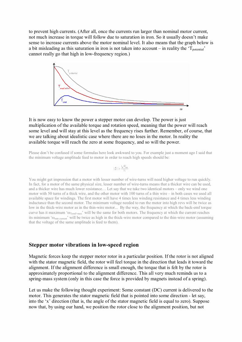
to prevent high currents. (After all, once the currents run larger than nominal motor current, not much increase in torque will follow due to saturation in iron. So it usually doesn’t make sense to increase currents above the motor nominal level. It also means that the graph below is a bit misleading as this saturation in iron is not taken into account – in reality the ‘Tpotential’ cannot really go that high in low-frequency region.)

It is now easy to know the power a stepper motor can develop. The power is just multiplication of the available torque and rotation speed, meaning that the power will reach some level and will stay at this level as the frequency rises further. Remember, of course, that we are talking about idealistic case where there are no loses in the motor. In reality the available torque will reach the zero at some frequency, and so will the power. Please don’t be confused if some formulas here look awkward to you. For example just a moment ago I said that the minimum voltage amplitude feed to motor in order to reach high speeds should be:

You might get impression that a motor with lesser number of wire-turns will need higher voltage to run quickly. In fact, for a motor of the same physical size, lesser number of wire-turns means that a thicker wire can be used, and a thicker wire has much lower resistance… Let say that we take two identical motors – only we wind one motor with 50 turns of a thick wire, and the other motor with 100 turns of a thin wire – in both cases we used all available space for windings. The first motor will have 4 times less winding resistance and 4 times less winding inductance than the second motor. The minimum voltage needed to run the motor into high revs will be twice as low in the thick-wire motor as in the thin-wire motor... By the way, the frequency at which the back-emf torque curve has it maximum ‘Temf=max’ will be the same for both motors. The frequency at which the current reaches its minimum ‘min current’ will be twice as high in the thick-wire motor compared to the thin-wire motor (assuming that the voltage of the same amplitude is feed to them). Stepper motor vibrations in low-speed region Magnetic forces keep the stepper motor rotor in a particular position. If the rotor is not aligned with the stator magnetic field, the rotor will feel torque in the direction that leads it toward the alignment. If the alignment difference is small enough, the torque that is felt by the rotor is approximately proportional to the alignment difference. This all very much reminds us to a spring-mass system (only in this case the force is provided by magnets instead of a spring). Let us make the following thought experiment: Some constant (DC) current is delivered to the motor. This generates the stator magnetic field that is pointed into some direction - let say, into the ‘x’ direction (that is, the angle of the stator magnetic field is equal to zero). Suppose now that, by using our hand, we position the rotor close to the alignment position, but not

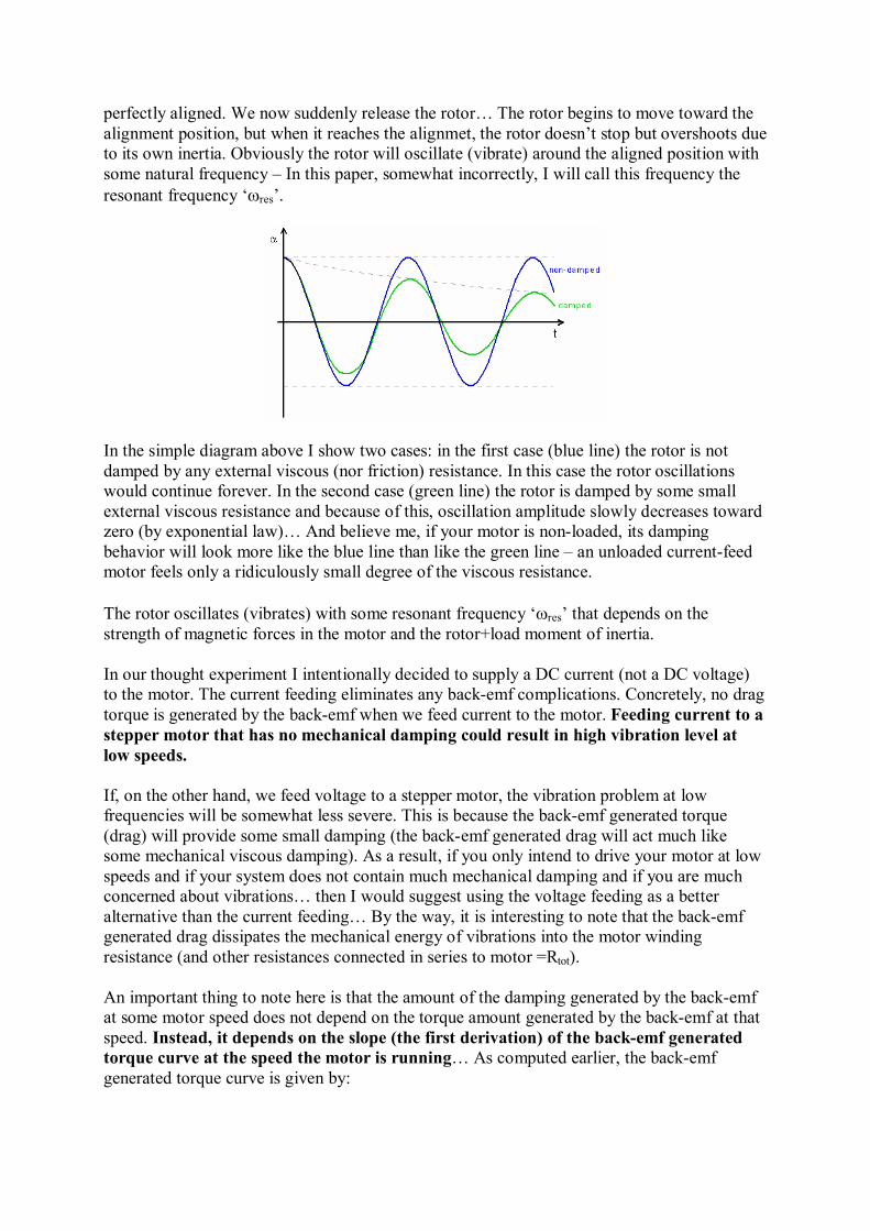
perfectly aligned. We now suddenly release the rotor… The rotor begins to move toward the alignment position, but when it reaches the alignmet, the rotor doesn’t stop but overshoots due to its own inertia. Obviously the rotor will oscillate (vibrate) around the aligned position with some natural frequency – In this paper, somewhat incorrectly, I will call this frequency the resonant frequency ‘res’.

In the simple diagram above I show two cases: in the first case (blue line) the rotor is not damped by any external viscous (nor friction) resistance. In this case the rotor oscillations would continue forever. In the second case (green line) the rotor is damped by some small external viscous resistance and because of this, oscillation amplitude slowly decreases toward zero (by exponential law)… And believe me, if your motor is non-loaded, its damping behavior will look more like the blue line than like the green line – an unloaded current-feed motor feels only a ridiculously small degree of the viscous resistance. The rotor oscillates (vibrates) with some resonant frequency ‘res’ that depends on the strength of magnetic forces in the motor and the rotor+load moment of inertia. In our thought experiment I intentionally decided to supply a DC current (not a DC voltage) to the motor. The current feeding eliminates any back-emf complications. Concretely, no drag torque is generated by the back-emf when we feed current to the motor. Feeding current to a stepper motor that has no mechanical damping could result in high vibration level at low speeds. If, on the other hand, we feed voltage to a stepper motor, the vibration problem at low frequencies will be somewhat less severe. This is because the back-emf generated torque (drag) will provide some small damping (the back-emf generated drag will act much like some mechanical viscous damping). As a result, if you only intend to drive your motor at low speeds and if your system does not contain much mechanical damping and if you are much concerned about vibrations… then I would suggest using the voltage feeding as a better alternative than the current feeding… By the way, it is interesting to note that the back-emf generated drag dissipates the mechanical energy of vibrations into the motor winding resistance (and other resistances connected in series to motor =Rtot). An important thing to note here is that the amount of the damping generated by the back-emf at some motor speed does not depend on the torque amount generated by the back-emf at that speed. Instead, it depends on the slope (the first derivation) of the back-emf generated torque curve at the speed the motor is running… As computed earlier, the back-emf generated torque curve is given by:

This curve has the steepest slope around the zero frequency (that is, zero speed) and this is where we can expect the most damping as a result of the back-emf. Unfortunately we cannot shape this curve any way we wish. The only parameter we can somewhat change is the ‘Rtot’. Adding a series resistor to motor winding is usually a bad idea – this would decrease the slope of the ‘Temf’ curve and thus it would decrease the damping effect. Furthermore, the resistor would dissipate lots of power. Still, under very rare circumstances adding a resistor could make some sense because it will push the ‘Temf’ curve maximum to higher frequencies thus extending the damping region toward higher frequencies and enabling your motor to reach a higher speed (at the expense of decreased torque) before high-frequency destructive vibrations develop. Can we decrease the ‘Rtot’ to create steepest curve and increase the damping effect? There is such a method, but it complicates the motor driver and thus the usability of this idea is questionable. The same method enables us to change the ‘Rtot’ to any value we want, and it can be done the following way: We continuously measure the current through windings; we then continuously adapt the voltage amplitude that we deliver to windings according to simple formula:

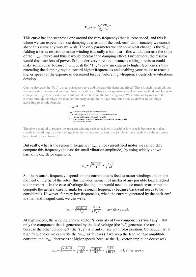
The above method to reduce the apparent winding resistance is only useful at low speeds because at higher speeds it would require more voltage than the voltage source can give (while at low speeds the voltage source has lots of reserve to give). But really, what is the resonant frequency ‘res’? For current feed motor we can quickly compute this frequency (at least for small vibration amplitude), by using widely known harmonic oscillator equations:

So, the resonant frequency depends on the current that is feed to motor windings and on the moment of inertia of the rotor (this includes moment of inertia of any possible load attached to the motor)… In the case of voltage feeding, one would need to use much smarter math to compute the general case formula for resonant frequency (because back-emf needs to be considered). However, for very low frequencies, when the current generated by the back-emf is small and insignificant, we can write:

At high speeds, the winding current vector ‘i’ consists of two components (‘i=iv+iemf’). But only the component that is generated by the feed voltage (the ‘iv’) generates the torque because the other component (the ‘iemf’) is in anti-phase with rotor position. Consequently, at high frequencies we can write the ‘res’ as follows (if we keep the feed voltage amplitude constant, the ‘res’ decreases at higher speeds because the ‘iv’ vector amplitude decreases).

As you can imagine, feeding voltage/current that has exactly the same frequency as the resonant frequency ‘res’ is going to provoke vibrations quickly. The same would also happen if you drive the motor with frequencies that are, say, one half or one third of the resonant frequency ‘res’. You can change the resonant frequency a bit by changing the current amplitude that you feed to the motor. Theoretically, if you need to drive the motor at some particular frequency and if it happens that this frequency is the resonant frequency, then you could avoid the resonance by either increasing or decreasing the current at that frequency. Well, I am not sure this could come good for any practical purpose because we are usually very limited about how much we can vary the current (we usually keep the current near the motor nominal current to get all the torque we can get). But it is good to know about it. The best way to keep away from vibrations at low frequencies is not to provoke them in the first place. That is, feed sine-wave (or microstep) to your motor instead of the square-wave. This way even some small damping, either mechanical or back-emf generated, should be enough to keep your motor performing acceptably. To recapitulate, you have several options to ease your low-frequency vibration problems:

- add some mechanical damping (Viscous type works better than friction type because the viscous damping can do the job even if the motor does not actually reverse its direction as it vibrates. You see, the friction damping type will not provide useful damping force because the friction force stays constant as long as the rotor moves in one direction regardless of its speed.)

- use sine-wave feeding or microstepping not to provoke vibrations - use voltage feeding to make use of the back-emf generated damping - never run the motor at frequencies that generate vibrations (jump over them) - carefully adjust current levels through motor windings to shift the resonant frequency

from particular frequencies you need to use (if you must run at exactly these speeds) - you can use simulated resistor ‘R*’ to increase the back-emf damping level by

increasing the slope of the back-emf generate torque curve (complex) - you can use more advanced regulators (even more complex)

At the end I must stress that the motor can and will vibrate with its resonant frequency at any rotation speed. Once you accelerate the motor over its resonant frequency, the driving voltage will not provoke much vibration any more, but any external disturbance will still cause vibrations at the resonant frequency. Stepper motor vibrations at medium frequency range While understanding low-frequency vibrations was easy, it took me some time to understand the instability that happens at the medium frequency range. In the lowest speed region motor vibrates because it is excited with signal whose frequency is close to the resonant frequency. However as frequency increases into the medium frequency region, if the motor is driven by voltage feeding, the motor again becomes unstable and is prone to lose steps.

Now, apparently out of blue, I made the above diagram. The diagram shows the back-emf generated torque curve (we discussed this curve in detail in the ‘back-emf’ chapter). I separated the frequency axis into four regions. The lowest region I call the “very low speed region” and I decided that this region ends at the frequency that matches the resonant frequency of the motor ‘res’. In this region the driving voltage signal is capable to provoke motor vibrations and we discussed these “low frequency vibrations” in the previous chapter. Once the driving voltage frequency increases over the resonant frequency it largely loses its ability to provoke low-frequency vibrations (but recall that the motor is always ready to vibrate at its resonant frequency if or when provoked by any other disturbance source). The next region I call the “low speed region” and here the motor mostly runs smoothly. This region ends at the frequency that matches the maximum of the back-emf generated torque curve. Note that in some rare cases the resonant frequency can be higher than the maximum back-emf torque frequency in which case this region would not exist. Next we have the portion I call the “medium speed region” where the back-emf generated curve has quite steep negative slope. This is where the motor will run unstable unless its load can provide enough viscous mechanical damping… At the end we reach the final region that I call the “high speed region”. The frequency at which the high speed region starts is not very strictly defined – in the high speed region the back-emf generated torque curve still has somewhat negative slope (but it is much more leveled now) and the motor that is running in this region regains its stability even if it is not purposely damped. Obviously, the instability of the medium speed region is caused by the strong negative slope of the back-emf generated torque curve. If you recall, we already discussed similar effect in the previous chapter were we said that at low frequency the large positive slope of the back-emf generated torque curve can assist us by creating viscous-like damping for our motor. In the medium frequency range exactly the same thing happens, only the viscous-like damping factor created by the back-emf is now negative. This means that in the medium speed range, instead of reducing vibrations (by exponential law), the back-emf will increase vibrations (also by exponential law). We calculated already the frequency where the back-emf generated torque curve has its maximum (that is, where the instability would start in the case of a totally non-damped motor). We also calculated the frequency where the back-emf generated torque curve has the steepest negative slope (that is where the motor will be the most unstable). If you recall, these frequencies are:

Practically there is noting that can be done to decrease the slope steepness of the back-emf generated torque curve. If your motor does not have enough external viscous damping it will become unstable. If you put some external mechanical viscous damping to the motor, very likely the damping agent will eat a major part of the motor available torque. Unpleasant… We can sometimes help ourselves a bit by adding some mass (moment of inertia) to the rotor. The added inertia might slow down the vibration development, and just maybe we will have the chance to speed up the motor into the high speed region where it can run continuously.

In the diagram above I wanted to depict what happens to a motor in the instability region. Motor’s actual speed, seemingly unprovoked, starts to oscillate around the commanded speed. The speed variations increase exponentially until the motor jumps out of synchronism, stalls or become erratic. The frequency at which motor’s speed oscillates is more or less equal to the motor resonant frequency ‘res’. The speed oscillation amplitude increases exponentially. (Oscillations will increase faster if the slope rate of the back-emf torque curve is more negative at this speed. If some external mechanical viscous damping is present, oscillations will increase slower – or not at all if enough viscous damping is present. Oscillations will also increase slower if more moment of inertia is attached to the rotor). Dense thin vertical lines represent step periods to make it clear that the frequency at which the speed oscillates is much lower than the stepping frequency. To get rid of the medium frequency range instability, you should not try to voltage-feed your motor in an open loop mode. Instead you should build a motor driver that uses current measurement feedback and a regulator that regulates the feed voltage accordingly. We will discuss briefly some techniques in the next chapter. Fighting medium frequency instabilities As we said, if you voltage-feed a stepper motor, you will not be able to fight instabilities in the medium frequency range unless you employ some feedback method. The easiest one to implement is to measure winding currents and then regulate the voltage accordingly… Below, I am again showing the stepper motor model (its ‘split’ version) so that we have it at our hand.

Here is one idea how to drive a motor and conquer the medium frequency vibrations… Our controller will compare the phase of the ‘Bv’ vector (see the above model) and compare it to the actual phase of the rotor position vector ‘’. The difference between these two positions (phases) is the ‘error’ value that our controller tries to minimize. Note that the actual rotor position ‘’ needs to be computed and we will do this from current measurements. Also note that the ‘Bv’ vector phase needs to be computed, but this computation is easier. Why did we choose such a regulator? In ideal conditions with no vibrations, the motor rotor vector ‘’ follow the ‘Bv’ vector. The rotor position might lag somewhat behind the ‘Bv’ vector phase depending on the load, but with a constant load and on constant speed this lag should remain constant. However when vibrations develop, the phase difference between the ‘Bv’ and ‘’ starts to oscillate with the resonant frequency ‘res’. We are going to oppose such oscillations; therefore our controller will not be sensitive to the absolute value of the phase difference between ‘Bv’ vector and ‘’ vector, but it will be sensitive to changes in the phase difference (that is, to the first derivation of the phase difference between ‘Bv’ and ‘’). The ‘Bv’ component of the stator magnetic field does not exist physically in the rotor. What really exist there is the compound stator magnetic field vector ‘B’ (B=Bv+Bemf). However, it is the ‘Bv’ component of this vector that mostly governs the rotor position. Recall that the ‘Bemf’ vector is small compared to the ‘Bv’ vector at low speeds. At high speeds, the ‘Bemf’ vector is mostly in anti-phase with the rotor position ‘’, so again its will only generate very small torque and not influence the rotor position much. The ‘Bemf’ vector has the greatest influence at the ‘Temf=max’ frequency where the back-emf torque curve has its maximum. But if we realistically presume that this frequency is much lower than the ‘min current’ frequency (this is where the ‘Bemf’ vector is approx. equal to the length as the ‘Bv’ vector) then we can safely say that across the whole frequency range it will be the ‘Bv’ vector that mostly influences the rotor position ‘’ and therefore our controller should work fine… Recall:

Now back to our controller… our controller will take rotation speed ‘ref’, which is an scalar, as an input value and will reproduce corresponding motor rotation (again, the ‘ref’ we are talking here is the motor full step-cycle frequency, 4 steps, not the actual shaft rotation speed). Our controller is depicted below (as you can se, it is somewhat complex – one part of its complexity is because it awkwardly mixes vector and scalar values, but even without that artificially introduced complexity, it would still be somewhat complex).

From the motor speed reference ‘ref’ (which is our leading value) we are computing the voltage phase reference ‘’ by simple integration. The voltage phase reference ‘’ is then used when computing the voltage reference vector ‘uref’. (The voltage reference vector ‘uref’ is further used to directly govern the voltage driver - not shown on the picture above). The voltage reference ‘uref’ vector has x and y components that can be computed as:

(Recall that the amplitude of the voltage reference vector must be adjusted at low frequencies to keep the motor current under the motor nominal current. However we are not investigating this detail here, we are just mentioning it. Here we are interested in the voltage reference vector phase: =+corr.) As you can see, when computing the reference voltage vector ‘uref’, we corrected its phase a bit by adding some small ‘corr’ parameter to the ‘’. This correction parameter is computed by our controller to keep the motor stable at the medium frequency range.

From the speed reference ‘ref’ we are also computing the phase of the ‘Bv’ vector (which is, by the way, the same as the phase of the ‘iv’ vector – refer to the stepper motor model at the beginning of this chapter). The phase of the ‘Bv’ vector can be computed using arctan function as:

Why do we compute the ‘Bv’ vector phase this way? The ‘Bv’ vector is directly under control of our feed voltage vector ‘u’ (refer to the stepper motor model) and the phase of the ‘Bv’ vector always follows the phase of the ‘u’ vector, that is, ‘’, only it is a bit retarded (up to pi/2 radians at high frequencies). How much it is retarded at some frequency only depends on the frequency and motor winding parameters, ‘R’ and ‘L’. Using some simple math we can obtain the above arctan formula. To show what I am talking about, I am extracting below this winding-related part from the stepper motor model:

Okay, this is how we computed the ‘Bv’ vector phase. Now we also need to compute the actual rotor position ‘’, and this is a bit harder task. As said, we are going to compute the rotor position from our current measurements. We would also need voltage measurements, but in practice no actual voltage measurements are necessary – almost always we already know internally what voltage we are supplying to the motor (this is actually equal to the ‘uref’ vector, if we suppose that our voltage driver does its job properly). To determine the rotor position ‘’, we must first compute the ‘emf’ vector. From our current measurements, we can compute the ‘emf’ vector’s x and y components the following way:

How did I obtain those formulas? From the stepper motor model we can see how the ‘u’, ‘emf’ and ‘i’ vectors are related. Just look again at the motor model and everything will be clear to you:

What I must stress is that current measurements should not contain too much noise! Fortunately, the next step to do is to integrate the ‘emf’ vector and this should somewhat reduce any present measurement noise. The notable exception is the offset error that would be slaughtering our chickens if present in the measured values. Major care should be taken about the offset error (bias) and therefore our next step, integrating the ‘emf’ vector, is not trivial. Instead of the pure integration, maybe a better choice would be passing the ‘emf’ vector through a low-pass filter that has the cutoff frequency much lower than the motor resonant frequency ‘res’. Such low-pass filter should take care about any small measurement bias, while still acting as an integrator at relevant frequencies. Unfortunately, even then we might have problems when motor is standing still or rotating very slowly because in this case the ‘emf’ vector will be zero or very near to zero and the low-pass filter that we are using for integration will drop to zero and the information about rotor position ‘a’ will be lost. Therefore, I would suggest considering the correction value ‘corr’ produced by our controller to be unreliable at very low frequencies and at stand still… Anyway, we integrate (or low-pass filter) the ‘emf’ vector:

The resulting vector ‘m*’ has the same phase as the rotor magnetic moment vector ‘m’, but does not necessarily has the same amplitude. We don’t care about its amplitude – we only care about its phase. The phase of the ‘m*’ vector is the same as the motor rotor phase ‘’ (refer to the motor model). Therefore our next step is to extract that phase from the ‘m*’ vector. We do this by using arctan function. However the standard arctan function would only give the result in –pi/2 to +pi/2 range, while we are interested in the –pi to +pi range.

The resulting computed phase of the rotor, ‘c’, has one big disadvantage – it is not a continuous phase, but a wrapped phase. This means that the computed phase will have discontinuities at –pi and +pi and will not be a continuous signal. We can try to unwrap the phase by signal tracking, but I would not recommend this. Instead, I would use the computed ‘c’ value despite the fact it is wrapped and compute the ‘error’.

The resulting ‘error’ signal is also going to be discontinued. I can now do several things with this discontinued error signal to prepare it for differentiation:

- I can make it continuous by applying sine function to it. We are ok to do this because the phase difference between the ‘Bv’ vector and the rotor position vector ‘’ should never exit the –pi to +pi range. In fact, treating the ‘error’ signal with the sine function my somehow smoother the error signal and the controller might behave better under high noise measurement conditions. Therefore, I can make:

- Or I can only make sure that the error value is within –pi to +pi range (by adding or by

subtracting 2*pi amounts until it is adjusted into the said range). Because the phase difference between the ‘Bv’ vector and the rotor position vector ‘’ is always somewhere within this range, we should not have problems with discontinuities.

- Or I do nothing and postpone the discontinuity problem into the next step, supposing that the next step is the pure differentiation (as shown on the controller model).

The next step, as shown in our controller model, is to make the ‘error’ signal differentiation. But you might also decide to use a full PID regulation here instead of a simple differentiation. If you ensured continuity of the ‘error’ signal you should not have problems with employing PID regulation, but I guess that your efforts might not show much improvement over a simple differentiator. The P component of a PID regulator might help at lower speeds (at frequencies lower than ‘min current’), but basically the D component is the one that is doing the real job here.

Using the differentiator-only regulation has one additional advantage – it is possible to use it even if the error signal is still discontinued: we compute the differential value as the current value minus previous value, and if the difference is larger than pi, we will subtract 2*pi; and if the difference is smaller than –pi, we will add 2*pi… If we implement our differentiator this way, we don’t have to ensure that the ‘error’ signal is always within the –pi to +pi range. This means that the ‘error’ signal does not have to be computed as the difference between rotor phase ‘’ and the ‘Cv’ vector phase; instead we could compute the ‘error’ signal as the difference between the rotor phase ‘’ and the voltage vector reference phase ‘’. This way we would not have to compute the ‘Cv’ vector phase. It is now time to low-pass-filter our differentiated ‘error’ signal. (We could, as an alternative, make the low-pass-filtering before we did the differentiation but only if we somehow ensured the continuity of the ‘error’ signal.) This low-pass filter cutoff frequency should be considerably higher (say 2 to 5 times higher) than the resonant frequency of the motor ‘res’. The purpose of this filtering is to reduce the measurement noise as much as possible wile not influencing the regulation abilities… Note that it is more effective to make noise filtration in the ‘error’ signal (or in its derivation) than to make noise filtration earlier, on the measured current signal. The reason is that currents change fast (with the stepping frequency), while the ‘error’ signal changes slowly (with the resonant frequency of the motor ‘res’). That’s why the cutoff frequency of the low-pass filter can be much lower if we filter the ‘error’ signal (or its derivation) than if we filter current measurements. At last, we multiply our differentiated-and-low-pass-filtered ‘error’ signal with a small constant (gain ‘Gd’) and we obtained our correction value ‘corr’ that is used to make correction to the voltage reference vector ‘uref’ phase. Note that very high ‘Gd’ gains could produce bad results, especially if high noise is present in measured currents. Aim for some reasonable gain. The correction value ‘corr’ may also be additionally conditioned:

- decreased or completely removed at low speeds due to low back-emf (low signal-to-noise ratios are therefore expected in the computed ‘emf’ signal at low speeds)

- increased at speeds that cause low-level vibrations because the described regulator can also fight low-level vibrations to some degree (if the differentiated ‘error’ signal is gained enough).

- decreased at speeds where the motor is naturally stable and does not need special care. We spent several pages describing our controller, but the question is can it be made simpler… We already said that if we implement the ‘error’ signal differentiator with some care so that it can differentiate also the wrapped phase signal, then we don’t need to compute the ‘Cv’ vector phase. Therefore:

Many of you immediately saw the opportunity to remove the integrator (or low-pass filter) that is integrating the ‘emfc’ vector. This is theoretically possible because all this integrator does is to phase-shift the signal 90 degrees behind. However, in practice this integrator is useful to control measurement noise, so removing it is only recommended if you can ensure that the current measurement has low noise. You certainly noticed that we are only interested in the phase of the ‘emfc’ signal (not in its amplitude) – this phase is related to the rotor position and this is what we want to stabilize. When you look more closely at the ‘emfc’ vector, you see that it is made of three components: ‘um’, ‘im * Rtot’ and ‘(dim/dt) * L’. The first component ‘um’ is actually more-or-less constant and does not carry any information about rotor vibrations. The second component ‘Im * Rtot’ would be an important component at low speeds, however at the problematic medium speed range (where >Rtot/L), the third component ‘(dim/dt) * L’ is more significant. We can, therefore, hope that the controller will still work at the medium speed range if we only include the third component of the ‘emfc’ vector. This enormously simplifies our controller because the current differentiator and the ‘emfc’ integrator cancels out. We get:

The simplified controller above can provide some stabilization at frequencies lower than ‘min

current’. What happens at the ‘min current’ is that the current here changes its phase for pi. What really happens at frequencies higher than ‘min current’ is that any change in rotor position phase will change the current vector phase in the opposite direction than it would be the case at frequencies lower than ‘min current’. Therefore, to compensate we should change the sign of the ‘Gd’ gain at frequencies higher than ‘min current’. Even this would not solve the problem how to pass the region where frequency is near the ‘min current’ and where motor currents are low (some fine tuning might help, I suppose)… This simplified controller could reach high speeds if the ‘min current’ is high enough so that at this frequency the motor already accelerated through the medium speed range and is now in the stable high-speed range. In any case I would suggest decreasing the gain ‘Gd’ toward zero as the frequency approaches toward ‘min current’. I would also suggest decreasing the gain ‘Gd’ toward zero at low frequencies (lower than ‘Temf=max’) where this simplified controller is ineffective. In our controller example we assumed continuous current measurements (taking the current sample as often as possible so that the later filter can reduce the noise effectively). But if current measurements are precise, then you might decide to take only one or two samples per step. This should work fine especially if the resonant frequency ‘res’ is relatively low (this is true if your motor is loaded with some significant inertial mass) compared to the stepping frequency. In fact, you might decide not to measure the winding current at all – you might only check, using a comparator circuit, the moment when the current in one winding crosses zero. Then, by observing the voltage reference phase ‘’ in that exact moment, you can directly find the phase difference (no need to use the nasty atan2 function). If you put two comparators (to monitor both winding currents) and if you trigger them at both, upward and downward current directions across the zero, then you can compare the phase four times in one cycle (that is, once per step). I probably missed something interesting and I probably made some mistakes in this paper. If you found anything like this, please write to me at: Danijel Gorupec, 2014 This document was prepared with help of the Math-o-mir software.