sticky swedes and flexible finns labour markets during the great
TRANSCRIPT
Sticky Swedes and Flexible Finns
Labour Markets during the Great Depression in Finland and Sweden
Sakari Heikkinen* and Christer Lundh
†
Paper presented at the European Historical Economics Society Conference, London 6th and 7th September 2013
ABSTRACT
Wage stickiness is a popular explanation for the greatness of the Great Depression. According to the sticky-wage explanation the slow adjustment of wages raised real wages above the market-clearing level causing reduction of output and labour, thus increasing unemployment. Explanations for wage stickiness are usually sought in the labour market institutions and their changes after the First World War. The complexity of the Great Depression makes it difficult to identify the role of the labour market institutions in cross-country comparisons. This paper examines the role of labour market institutions by comparing Finland and Sweden. The design of the study builds on the comparison of two countries with great similarity with respect to the economic structure and trade pattern, monetary policy, but with two kinds of industrial relations systems; the study thereby has the form of a natural experiment. Results indicate that stronger trade unions and collective bargaining made wages stickier in Sweden, while in Finland where collective agreements did not exist and unions were weaker wage adjustment was more flexible.
* Department of Political and Economic Studies, University of Helsinki, Finland e-mail: [email protected]. † Department of Economy and Society, University of Gothenburg, Sweden e-mail: [email protected].
2
1. Introduction
The role of labour markets in the Great Depression has been debated a lot. Sticky nominal wages is
an explanation that has been often listed among the major causes of the greatness of the depression
– both its depth and its length. According to the sticky-wage explanation the slow adjustment of
wages raised real wages above the market-clearing level, to which employers responded by cutting
their labour force. Explanations for wage stickiness, again, are usually sought in the labour market
institutions and their changes after the First World War. The growth of membership in trade unions,
the spread of collective bargaining and the increasing coverage of unemployment benefits are key
themes in the discussion.
The complexity of the Great Depression makes it difficult to identify the role of the labour
market institutions in cross-country comparisons, since the course of the depression depended on
several other factors, e.g. the differing decisions made in monetary and exchange-rate policy. In this
respect Finland and Sweden offer us an interesting case for comparison since the countries were in
many respects similar during the Great Depression. Both were small open economies with high
exports/GDP ratio and the UK as the main export market. Furthermore, both countries followed
Britain in autumn 1931 and left the gold standard. Yet there was one major difference between
Finland and Sweden – the labour market institutions influencing wage formation were quite
different. In Sweden collective bargaining was predominant in the industrial labour market, whereas
there were no collective agreements in Finland, where trade unions were very weak compared to
Sweden. Since the collective agreements typically were valid for longer periods, the collective
bargaining system constrained rapid wage reduction in Sweden, while in Finland there were no
similar obstacles for a rapid wage adjustment. When it comes to unemployment benefits, neither
country had publicly financed unemployment insurances during the depression (it was introduced in
Sweden in the beginning of 1935). Yet there were trade-union-based unemployment benefit
schemes in both countries. Since the unionization rate was notably higher in Sweden and unions
stronger than in Finland, it could be assumed that also in this respect labour markets were – from
the employer point of view – more flexible in Finland than in Sweden.
Finland and Sweden, thus, provide us with a natural experiment on the effect of labour market
institutions on the course of the Great Depression. The paper compares the development of nominal
and real wages in manufacturing industries in Finland and Sweden. It is organised as follows. First
we outline the discussion on wage stickiness in the Great Depression literature. Thereafter (section
3) we compare the labour market institutions of Finland and Sweden. Section 4 outlines the
development of Finnish and the Swedish manufacturing industries over the Great Depression.
3
Section 5 compares the development of labour-market quantities – employment and working hours.
Thereafter we examine prices: the development of nominal wages (section 6) and real wages
(section 7) in Finnish and Swedish manufacturing industries. Section 8 puts quantities and prices
together and compares labour market dynamics in depression and recovery. Section 9 concludes the
paper.
2. Wage stickiness and the Great Depression: approaches and puzzles
Sticky wages loom large in the literature of the Great Depression. Yet, despite its popularity of the
as an explanation for the gravity of the depression the stickiness of nominal wages is still quite a
puzzle. According to Ben S. Bernanke “the incomplete adjustment of nominal wages to price
changes” is difficult to reconcile “with the postulate of economic rationality”. He states that “[w]e
cannot claim to understand the Depression until we can provide a rationale for this paradoxical
behavior of wages”.1
Explanations for this paradox have been sought by applying various approaches. First, there
are studies focusing on individual economies, especially on USA (e.g. Bernanke 1986; Bordo et al.
2000) and UK (e.g. Dimsdale et al. 1989) but also on Sweden (Fregert 2000). Second, many cross-
country comparisons have measured the extent and effects of wage stickiness (e.g. Eichengreen &
Sachs 1985; Bernanke & James 1991; Bernanke & Carey 1996; Madsen 2004).2 Between these
approaches there is a trade-off between depth and breadth: it is difficult to generalize on the basis of
a one-country study, whereas it may be hard to take into account the complexities of the depression
in a multi-country study.3 The third approach is the middle way between these: a two-country
comparison. This has been applied recently by Timothy J. Hatton and Mark Thomas (2013) in their
comparative study on labour markets in the UK and USA in the 1920s and 1930s. They have argued
“that labour market outcomes are the result of the interaction between shocks and institutions”.4
This is also our approach: we compare labour markets in manufacturing industries in Finland and
Sweden from 1926 to 1938. In one important respect our pair of countries is different from the one
used by Hatton and Thomas. Since the decisions of UK and USA were different during the
depression in monetary and exchange-rate policy, the role of labour market institutions might be
1 Bernanke 1995, p. 2. 2 Both Finland and Sweden are included in the samples of Eichengreen & Sachs and Madsen, whereas only Sweden belongs to data sets of Bernanke & James and Bernanke & Carey. 3 Exceptions normally end up categorized as outliers as Finland in both Eichengreen’s and Sachs’ and Madsen’s regressions. 4 Hatton & Thomas 2013, p. 344.
4
harder to identify than in the case of Finland and Sweden, both leaving the gold standard and
depreciating their currencies already in the autumn 1931.
The sticky-wage literature involves many measurement problems. The comparability of wage
data in cross-country studies is a potential problem, since it is not always clear that the definitions
of available wage statistics are similar from one country to another. Nominal “wage” can mean at
least two different things: tariff wage or the actual average wage. Different wage systems – hourly
of piecework pay – complicate the picture further. When we move from nominal to real wages the
choice of deflator is crucial. The best solution should be the use of consumer price indices (CPI) for
calculating real consumption wages and industry-specific producer price indices (PPI) for real
product wages. Much of the literature has, though, relied on wholesale price indices (WPI),
although they – as Madsen (2004) has pointed out – are biased for the purpose. A further limitation
of some of the studies, as Bernanke (1986) has noted, is the use of highly aggregated data and
ignoring such an important variable as the length of the workweek.
We have aimed at avoiding the data problems mentioned above. We have collected from both
countries data that is so far as possible comparable. We are convinced that our data on wages for
Finland and Sweden is of better quality than data of any of the former studies.5 We have
disaggregated manufacturing into same six major industries in both countries representing over 80%
of the total. Disaggregation is important, since demand shock was quite different in export- and
home-market oriented industries. We have constructed series of nominal wages as well as on both
real consumption wages and real product wages. Our labour input data consists of series of
employment and average working hours.
All in all, our data set on six manufacturing industries consists of following variables: 1)
output (Q), 2) employment, i.e. the number of workers (N), 7) average annual working hours (H), 4)
nominal hourly wages (W), 5) producer prices (P), 6) real consumption wages (RCW=W/CPI), 7)
real product wages (RPW=W/P). Furthermore, from these variables we have derived 8) labour input
(L=E∙N), 9) real annual earnings (RAE=RCW∙H) and 10) labour productivity (Q/L).
3. Labour market institutions in Finland and in Sweden in the 1920s and the 1930s
In Sweden local trade unions were formed from the late 1860s, nation-wide trade unions from the
1880s, and the national confederation of trade unions (Landsorganisationen, LO) in 1898.6 As a
response to workers’ unionism employers’ associations were organized nationally by trade and in a
5 However, we have to content ourselves on annual data since there is no more frequent data on all the variables. 6 The description of the Swedish labour market is based on Lundh 2008 and 2010.
5
joint confederation (Svenska Arbetsgivareföreningen, SAF) in 1902. In the 1890s and early 1900s,
employers’ organizations, e.g. in the sawmill industry, opposed the right of trade unions to negotiate
and make agreements on behalf of the workers. However, after a period of conflicts the institution
of collective bargaining and agreements was finally accepted by the Swedish employers’
associations in the big industry. Its final adoption was confirmed by a nation-wide collective
agreement in the engineering industry in 1905 and a general agreement on industrial relations
between the LO and the SAF in 1906. From then conflicts between organized labour and employers
concerned wages and working conditions for the next contract period, disputes over how
agreements that were in force should be interpreted, and issues of prospective violation of valid
agreements; the principle of collective bargaining itself was not questioned.
Collective bargaining was adopted typically at the national level in the interwar period, and
agreements were made between nation-wide trade unions and employers associations. Local trade
unions controlled negotiations though. Proposal of national agreements had to be circulated for
ballot in the local trade unions, and once accepted the national agreement had to be adapted to firm
specific situation in negotiations between the firm and the local trade union. This system made it
difficult for labour leaders taking part in the bargaining to back off from aggressive union demands
and take a more moderate stand when new facts were shown on rising production costs or
increasing trading problems; they knew that they would risk being outvoted. In the latter half of the
1930s the ballot system was gradually abandoned and replaced by a system of more centralized
bargaining.7
How to handle a dispute over the interpretation or violation of an agreement, including a
blockade, strike or lockout during the contract period, was partly regulated in the general agreement
between the LO and the SAF, and partly in the early labour legislation on voluntary state mediation.
In 1928 a new and more forceful labour legislation was adopted by the Swedish parliament. A
national labour court was implemented with representatives of the trade unions, employers’
associations and the state (jurists), which should mediate in disputes over the content or
interpretation of an agreement in force. The court could decide to fine the party that had violated the
agreement (by abandoning what it stipulated or by starting a conflict before the contract period had
ended).8 The system invented in 1928 mainly aimed at reducing the number of strikes which was
high in the 1920s; however it also made it more costly for employers to make changes in wages or
working conditions that may have been made necessary due to external economic shocks like the
Great Depression.
7 Lundh 2008, pp. 60, 107; Lundh 2012, pp.190–91. 8 Lundh 2010, pp. 132–34, Göransson 1988, pp. 201–09.
6
The length of contracts periods varied over time and trades, and the endpoints/starting points
of contract periods were not synchronized between industries. In 1908–1917 contract periods were
on average quite long, about half being valid for two years or more.9 As a result of the depression in
the early 1920s periods became shorter. In 1918–1927 the proportion of one-year contracts was
82% and of two-year contracts 15%. In the late 1920s contract periods started to become longer
again, peaking in 1930 when about 50% of the collective agreements were due for one year, 40%
for two years, and the rest for three years. The Great Depression had the same effect on contract
periods as the depression in the 1920s, length of the periods shrank. In 1933 80% of the collective
agreement were in force for one year (or less), and 15% for 1–2 years. As the Depression gave way,
duration of contracts grew. In 1938 52% of the contracts were for one year (or less), and 45% for 1–
2 years. Thus, in the interwar period we find a clear pro-cyclical pattern: contract periods were
longer when business was busy and shorter in times of economic crisis.
In the 1920s, about one third of blue collar workers in industry were union members, a
proportion that increased to half in the mid-1930s and two thirds in 1940. Unions tried to enforce
collective agreements in trades were they were strongly organized, both with enterprises that were
members of an employer association and with those who were not yet organized. In this way, the
organization of employers increased. Also, the large number of strikes and some big lockouts in the
1920s and early 1930s encouraged workers to become union members (in order to get strike
allowances) and unorganized employers to take up membership in an employers association (in
order to get subsidies during strikes). Great union density and a large number of workers in firms
that were members of an employer association is thus one part of the background of the large
coverage of the collective agreement in Sweden in the interwar period.10 In addition, both parties
were of one opinion that the collective agreements should be valid for all workers of the trade who
were working in the firm in question, not only for the trade union members. Therefore collective
agreements set the standard of wage level and working conditions for a larger number of workers
than those who were unionized. During the period 1926–1938, about 8–14% of the workers covered
by collective agreements (made by a trade union belonging to the LO) we unorganized.11
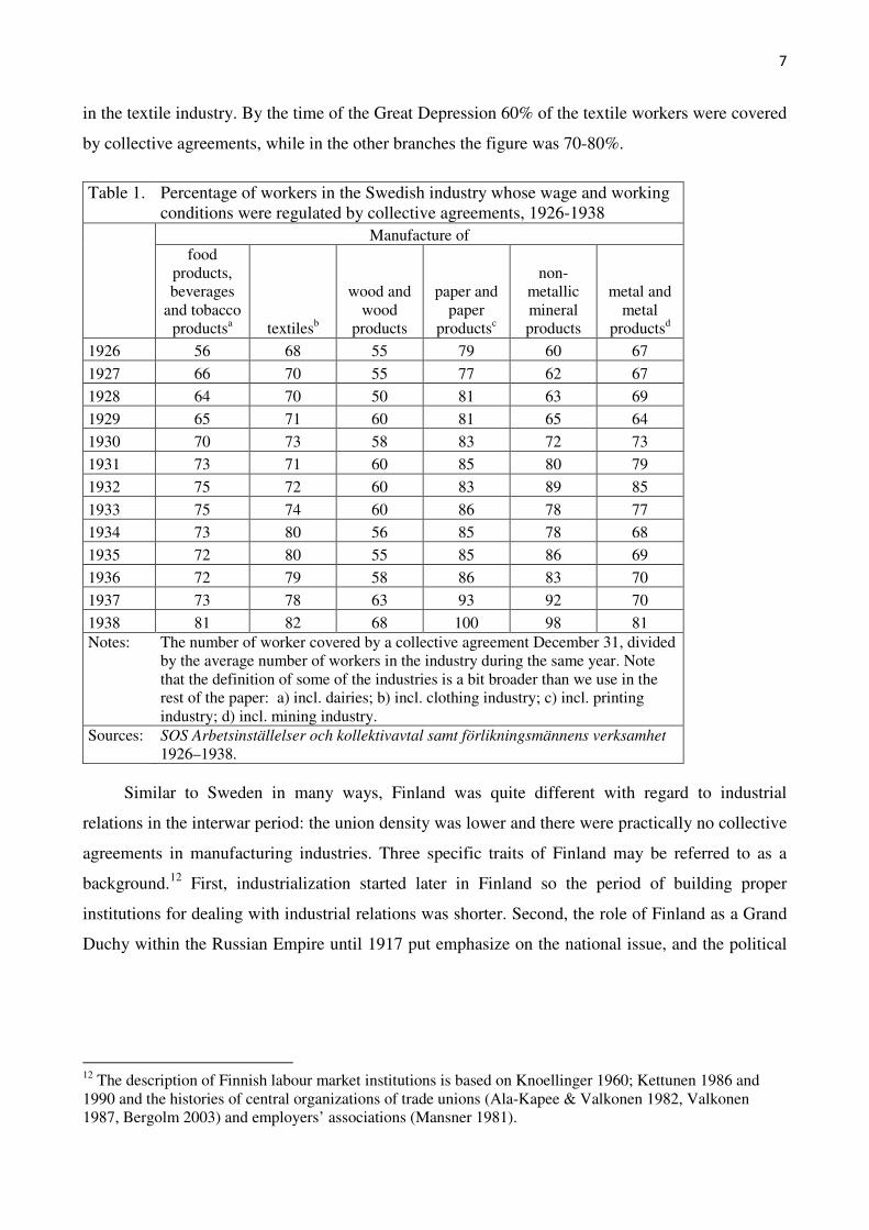
It has been estimated that the coverage of collective agreements in Swedish industry were on
average over 70% in 1930 and more than 80% in 1938. As can be seen in Table 1 the variation in
coverage was substantial. The greatest coverage could be found in the paper industry and the least
9 Arbetsinställelser och kollektivavtal samt förlikningsmännens verksamhet 1938: 31. 10 Lundh 2008, pp. 81–85, 140–41. 11 LO:s verksamhetsberättelse, 1926–1938.
7
in the textile industry. By the time of the Great Depression 60% of the textile workers were covered
by collective agreements, while in the other branches the figure was 70-80%.
Table 1. Percentage of workers in the Swedish industry whose wage and working conditions were regulated by collective agreements, 1926-1938
Manufacture of
food products, beverages
and tobacco productsa textilesb
wood and wood
products
paper and paper
productsc
non-metallic mineral products
metal and metal
productsd
1926 56 68 55 79 60 67
1927 66 70 55 77 62 67
1928 64 70 50 81 63 69
1929 65 71 60 81 65 64
1930 70 73 58 83 72 73
1931 73 71 60 85 80 79
1932 75 72 60 83 89 85
1933 75 74 60 86 78 77
1934 73 80 56 85 78 68
1935 72 80 55 85 86 69
1936 72 79 58 86 83 70
1937 73 78 63 93 92 70
1938 81 82 68 100 98 81
Notes: The number of worker covered by a collective agreement December 31, divided by the average number of workers in the industry during the same year. Note that the definition of some of the industries is a bit broader than we use in the rest of the paper: a) incl. dairies; b) incl. clothing industry; c) incl. printing industry; d) incl. mining industry.
Sources: SOS Arbetsinställelser och kollektivavtal samt förlikningsmännens verksamhet 1926–1938.
Similar to Sweden in many ways, Finland was quite different with regard to industrial
relations in the interwar period: the union density was lower and there were practically no collective
agreements in manufacturing industries. Three specific traits of Finland may be referred to as a
background.12 First, industrialization started later in Finland so the period of building proper
institutions for dealing with industrial relations was shorter. Second, the role of Finland as a Grand
Duchy within the Russian Empire until 1917 put emphasize on the national issue, and the political
12 The description of Finnish labour market institutions is based on Knoellinger 1960; Kettunen 1986 and 1990 and the histories of central organizations of trade unions (Ala-Kapee & Valkonen 1982, Valkonen 1987, Bergolm 2003) and employers’ associations (Mansner 1981).
8
part of the labour movement was in Finland more important than the trade unions.13 Third, and the
most important cause, were the repercussions of the Finnish Civil War in 1918.
Local trade unions appeared in Finland in the late 19th century, and nation-wide unions were
formed in the early 20th century including a federation of trade unions (Suomen Ammattijarjestö,
SAJ) in 1907. In the same year also employers founded their own central confederation (Suomen
Tyonantajain Keskusliitto, STK), preceded by the formation of trade-based national employer
associations. Organizational foundations for collective bargaining were thus created, and Finland
seemed to follow the example of e.g. Sweden in the evolution of labour market institutions.
Printers’ union succeeded in 1900 getting a nation-wide collective agreement starting a practice that
continued until 1935. Printers’ agreement was the only nation-wide, but there were important local
collective agreements e.g. in the metal industry in 1906 and the paper industry in 1907.14
Trade union movement in Finland grew during periods of revolution in Russia, e.g. in 1905,
but shrank as the Russian state became stronger again. In 1917, after the February revolution, the
number of union members increased rapidly and the union density in manufacturing industries
peaked at 27% in 1920.15 Although the number of members had increased there were several factors
eroding the power of trade unions – both from the inside and the outside. The troubles of the trade
unions stemmed from the Finnish Civil War in 1918, which ended in the defeat of the “reds”. Since
trade unions had a close relationship with the political labour movement also their position was
undermined.
Employers’ associations representing the big industry were after the Civil War against
collective bargaining even more unflinchingly than before. They opposed seeing trade unions as a
representative for the collective of workers, instead they were in favour of firm-specific industrial
relations between the industrialist and the individual workers. Trade unions they considered as a
third party without legal rights to intervene. Despite labour conflicts on the matter in 1927–1929,
big industry withheld its resistance towards collective bargaining; no new collective agreements
were made in the manufacturing industries in the interwar period leaving printing industry the
exception proving the rule. Collective bargaining was practised in other industries (e.g. building) on
an irregular basis depending on the strength of the trade unions and the needs of the employers. A
wave of collective agreements appeared in 1919–1920 and another one in 1926–1927. In
manufacturing industries, however, employers did not back down.
13 The relative weakness of trade unions, however, can be interpreted also as a relative strength of the political labour movement; see Kettunen 1990, p. 135. 14 Ala-Kapee & Valkonen 1982, pp. 79–177; Bergholm 2003. 15 Kettunen 1986, p. 142.
9
A result of the Civil War was the split of the Finnish labour party into Social Democrats and
Communists. The rivalry between the two parties was very intense within the trade unions in the
1920s. As communist gained power in trade unions employers’ attitude towards unions became
harsher. Finally these inner and outer pressures broke the Finnish federation of trade unions (SAJ)
in 1929–1930. First social democrats left SAJ in 1929 and one year later the government dissolved
SAJ on political grounds, as a communist organization. Social democrats founded in October 1930
a new federation of trade unions (Suomen Ammattiyhdistysten Keskusliitto, SAK).16
At the onset of the Great Depression Finnish trade unions were at a historically low point. In
1928, the union density in manufacturing industry was 26% but in 1930 only 8%.17 The share of
those covered by collective agreements was only a few percents (i.e. workers of printing industry).
After the depression the membership of trade unions increased rapidly, but collective bargaining
remained to the end of the decade an unattainable goal.18 However, as public opinion grew more
positive towards collective agreements, employers’ central organization (STK) considered it
necessary in the end of the 1930s to defend its negative attitude towards collective agreements by
publishing pamphlets on the question. One central reason for opposing collective agreements
presented was that they prohibited business life from flexibly adjusting to business cycles.19 During
the Great Depression there were no such institutional obstructions for “flexible adjustment” in
Finland, whereas in Sweden they were notable.
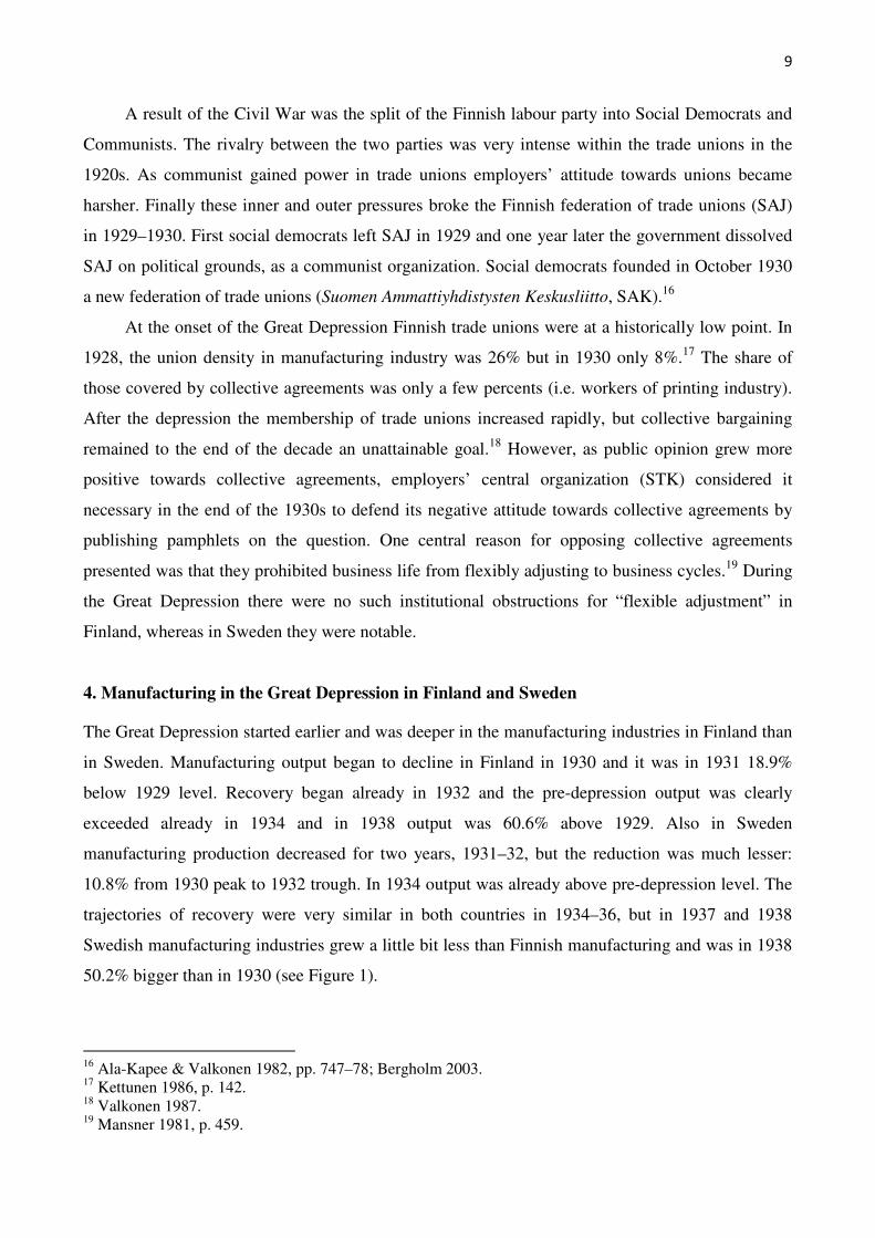
4. Manufacturing in the Great Depression in Finland and Sweden
The Great Depression started earlier and was deeper in the manufacturing industries in Finland than
in Sweden. Manufacturing output began to decline in Finland in 1930 and it was in 1931 18.9%
below 1929 level. Recovery began already in 1932 and the pre-depression output was clearly
exceeded already in 1934 and in 1938 output was 60.6% above 1929. Also in Sweden
manufacturing production decreased for two years, 1931–32, but the reduction was much lesser:
10.8% from 1930 peak to 1932 trough. In 1934 output was already above pre-depression level. The
trajectories of recovery were very similar in both countries in 1934–36, but in 1937 and 1938
Swedish manufacturing industries grew a little bit less than Finnish manufacturing and was in 1938
50.2% bigger than in 1930 (see Figure 1).
16 Ala-Kapee & Valkonen 1982, pp. 747–78; Bergholm 2003. 17 Kettunen 1986, p. 142. 18 Valkonen 1987. 19 Mansner 1981, p. 459.
10
The depression was longer in manufacturing employment than in output in both countries.
The number of manufacturing workers in Finland diminished by 24.6% from the 1928 peak to the
1932 trough. In Sweden the manufacturing workforce decreased by 13.1% from 1930 to 1933.
Measured in employment the depression was in Finland, relative to Sweden, even deeper than when
measured by output. The rebound of employment began (in annual figures) a year later than of
output – in 1933 in Finland and in 1934 in Sweden. The pre-depression employment was surpassed
both in Finland and in Sweden in 1935. The number of workers grew along with the output but at a
slower rate implying that also productivity grew. In 1938 the number workers employed in
manufacturing industries was in Finland 27.8% and in Sweden 19.5% above pre-depression level.20
20 We have applied the definition of manufacturing used in contemporary Finnish and Swedish manufacturing statistics (very similar in both countries). The statistics don’t include industrial handicraft, which is counted in historical national accounts (HNA) of Finland (Hjerppe 1989) and Sweden (Schön & Krantz 2012). According these statistics the total of manufacturing (i.e. handicraft included) output diminished in the depression 16.5% in Finland and 11.5% in Sweden. Employment contracted 18.4% in Finland and 9.5% in Sweden. Part of the differences in employment figures is explained also by the fact that we examine only production workers, whereas HNA figures include also salaried employees. We have used the narrower definitions of manufacturing industry and employment for three reasons. First, our wage and working-hours data concern only production workers in manufacturing industry proper. Second, even if there
50
60
70
80
90
100
110
120
130
140
150
160
170
1926 1928 1930 1932 1934 1936 1938
1929=100
Note: White-collar employees are not included.
Sources: see Appendix 1.
Figure 1. Manufacturing output and employment in
Finland and Sweden, 1926–1938
Sweden, output Sweden, workers
Finland, output Finland, workers
11
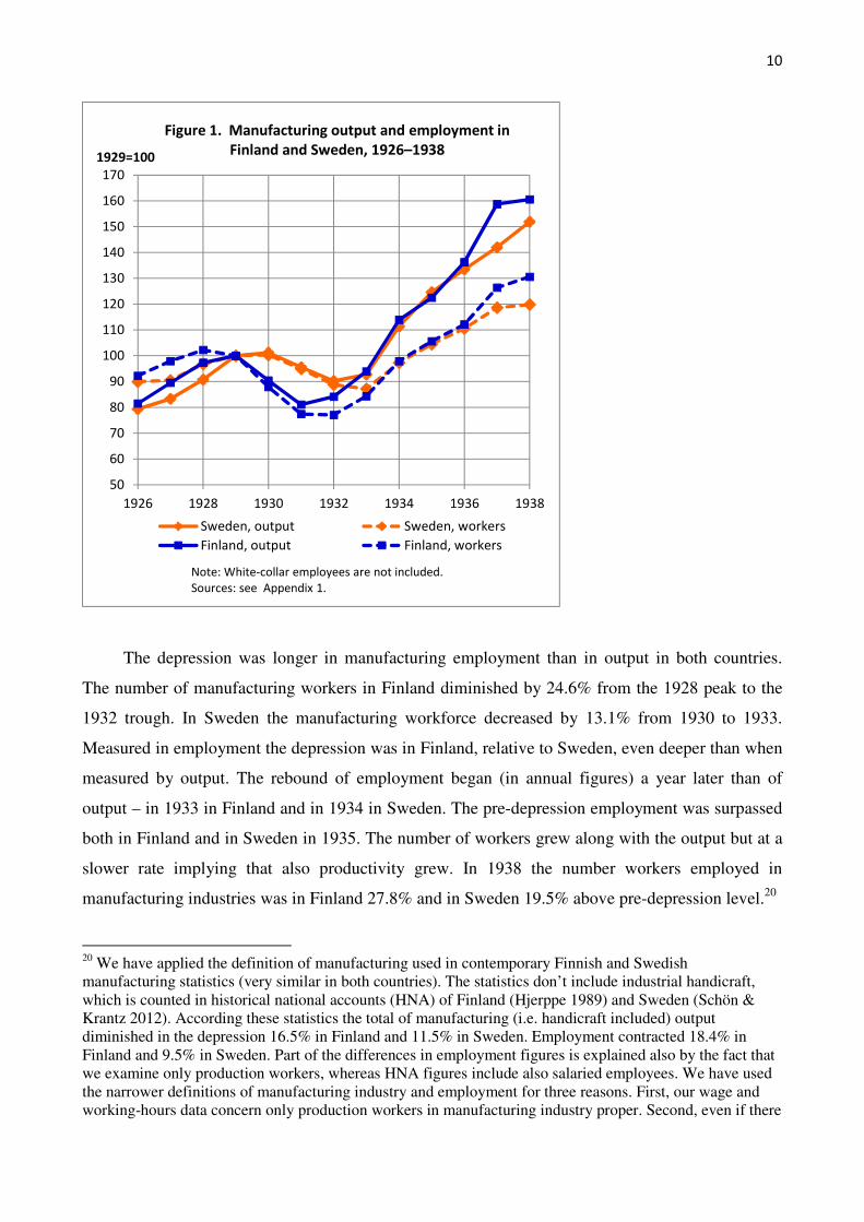
There were, thus, many similarities in the development of the Finnish and Swedish
manufacturing industries during the Great Depression. Yet there was also a significant difference in
that the depression was notably milder in the Swedish manufacturing compared to the Finnish one.
Partly this difference could be explained by differences in the structure of manufacturing industries
(see Table 1). Wood and paper product industries were the dominating industries in Finland. They,
furthermore, were the only notable export industries; all the other manufacturing industries sold
their products in practice solely to the domestic market. In Sweden metal manufacturing was the
major industry. It was also, in contrast to Finland, an important export industry, besides of which
wood and paper industries were export-oriented too. Therefore, the declining demand of sawmill
products from 1929 onwards hit much harder the Finnish than Swedish manufacturing (employment
shares of wood manufacturing being 31.3% and 15.4% respectively in 1928). The other three major
manufacturing industries (textile manufacturing; food, drink and tobacco industries; the
manufacture non-metallic mineral products, e.g. glass, cement and porcelain) were in both countries
domestic-market industries. These six industries made more than 80% of the total employment of
manufacturing in both countries (see Table 2). The analysis in the following focuses on these six.
Table 2. The structure of manufacturing workforce in Finland and in Sweden 1928, 1932 and 1938, %
Finland Sweden
1928 1932 1936 1928 1932 1936
Manufacture of food products, beverages and tobacco products (FOOD) 7.0 8.1 7.1 9.2 9.7 8.4
Manufacture of textiles (TEXTILE) 9.8 11.2 11.3 10.3 11.2 10.6
Manufacture of wood and wood products (WOOD) 31.3 24.5 25.2 15.4 13.2 12.8
Manufacture of paper and paper products (PAPER) 11.0 13.4 11.4 10.1 10.4 8.8
Manufacture on non-metallic mineral products (MINERAL) 6.5 5.7 6.5 10.0 8.8 7.8
Manufacture of metal and metal products (METAL) 17.4 18.0 19.3 28.8 28.9 34.2
Other manufacturing industries* 17.0 17.5 17.3 16.1 17.7 17.4
ALL MANUFACTURING INDUSTRIES 100.0 100.0 100.0 100.0 100.0 100.0
Note: Salaried employees and proprietors are not included. * Mining and electricity, gas and water services are not included.
Sources: See Appendix 1.
were comparable data on salaried employees, they constituted in the interwar years a group economically and socially were different from workers. Third, handicraft data are poorer quality than the contemporary manufacturing statistics. Therefore handicraft series in HNA are to a great extent based on estimations, which weakens their usability for the cyclical analysis of production and employment.
12
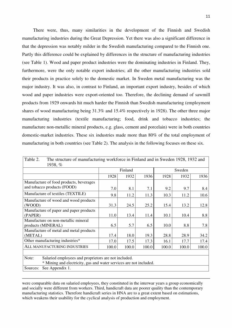
Figure 2. Output of six major manufacturing industries in Finland and in Sweden, 1926–1938 (1929=100)
50
60
70
80
90
100
110
120
130
140
150
160
170
180
1926 1928 1930 1932 1934 1936 1938
Food
Sweden Finland
5060708090
100110120130140150160170180190200210220
1926 1928 1930 1932 1934 1936 1938
Textile
Sweden Finland
50
60
70
80
90
100
110
120
130
140
1926 1928 1930 1932 1934 1936 1938
Wood
Sweden Finland
5060708090
100110120130140150160170180190200210
1926 1928 1930 1932 1934 1936 1938
Paper
Sweden Finland
50
60
70
80
90
100
110
120
130
140
150
160
170
180
1926 1928 1930 1932 1934 1936 1938
Mineral
Sweden Finland
50
60
70
80
90
100
110
120
130
140
150
160
170
180
190
1926 1928 1930 1932 1934 1936 1938
Metal
Sweden Finland

13
A quick comparison by industry (see Figure 2) shows that with the exception of paper
industry manufacturing output diminished during the depression more in Finland than in Sweden.
The recovery trajectories were also quite similar, although paper industry was again an exception:
the growth of output was in Finland significantly quicker than in Sweden. Also food21, textile and
mineral industries production grew in Finland somewhat quicker than in Sweden, whereas the
Swedish metal industry clearly outperformed the Finnish. Recovery was quite modest in wood
industry of both countries: output barely reached the pre-depression level in the end of the 1930s.
5. Employment and working hours
As output diminished manufacturing industries needed less labour input than before (assuming that
labour productivity did not change). This could be done either by cutting workforce or reducing
working hours per worker – or by combining both methods. How did employment (number of
workers) adjust to the decline of output? This has been displayed industry by industry and over the
years in Figure 3 and from peak to trough relative to the decline of output in the left-hand graph of
Figure 5.
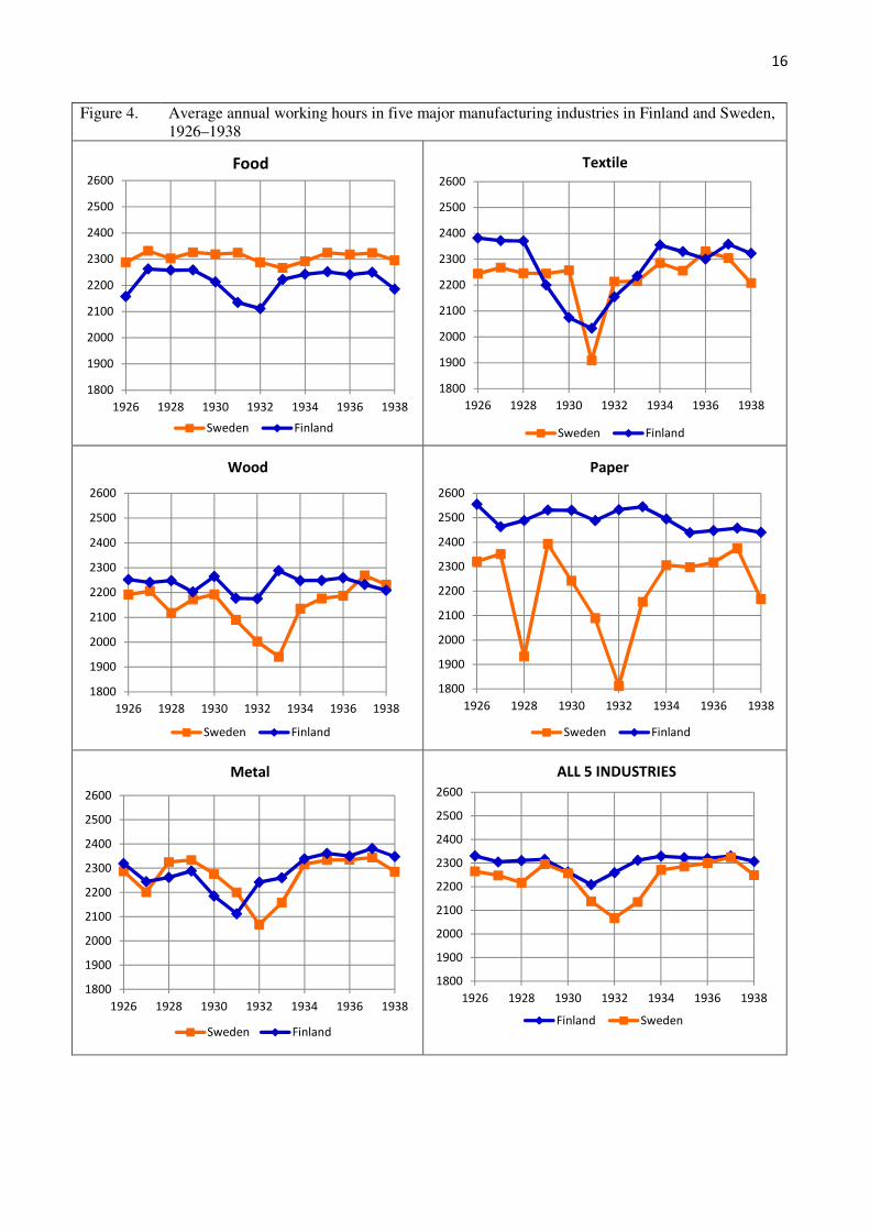
Figure 3 shows that there were no systematic difference between Finland and Sweden in
reducing labour force, given the differences in output (Figure 2). This conclusion is confirmed by
the left-hand panel of Figure 5, which plots the number of workers (vertical axis) against the output
(horizontal axis) in the six major manufacturing industries. The diagonal shows the line, where
employment diminished in step with output – below it the number of workers decreased more than
output and above it the cutback in employment was lesser than in output. First observation to be
made is that Swedish manufacturing industries were in general closer than the Finnish industries to
the diagonal, i.e. the reduction in manufacturing employment did not differ significantly from the
decline in output. Secondly, the variation between industries was greater in Finland than in Sweden.
In some industries (e.g. wood manufacturing) employment was cut much more than in Sweden
relative to output decline, but the reverse was true in some other industries (e.g. metal
manufacturing). All in all, the figure implies that there was no systematic difference between
Finland and Sweden in the industrial labour market “flexibility” in this respect: the number of
workers was reduced in both countries on average in step with the declining output. The similarity
of employment contracts is the natural explanation for this, since the normal term of notice was two
weeks in Finland and about the same in Sweden,
21 The growth of Finnish food, beverage and tobacco industries since 1933 resulted from the rapid growth of manufacture of beverages, which again was is to be credit to the abolishment of alcohol prohibition in 1932. The output of food and tobacco industry was in 1938 only 30% above 1929 level, much less than 67% growth of the total with manufacturing of beverages included.

14
Figure 3. Employment in six major manufacturing industries in Finland and in Sweden, 1926–1938 (1929=100)
50
60
70
80
90
100
110
120
130
140
150
1926 1928 1930 1932 1934 1936 1938
1929=100 Food
Sweden Finland
50
60
70
80
90
100
110
120
130
140
150
1926 1928 1930 1932 1934 1936 1938
Textile
Sweden Finland
50
60
70
80
90
100
110
120
130
140
150
1926 1928 1930 1932 1934 1936 1938
Wood
Sweden Finland
50
60
70
80
90
100
110
120
130
140
150
1926 1928 1930 1932 1934 1936 1938
1929=100 Paper
Sweden Finland
50
60
70
80
90
100
110
120
130
140
150
1926 1928 1930 1932 1934 1936 1938
1929=100 Mineral
Sweden Finland
60
70
80
90
100
110
120
130
140
150
160
1926 1928 1930 1932 1934 1936 1938
Metal
Sweden Finland
15
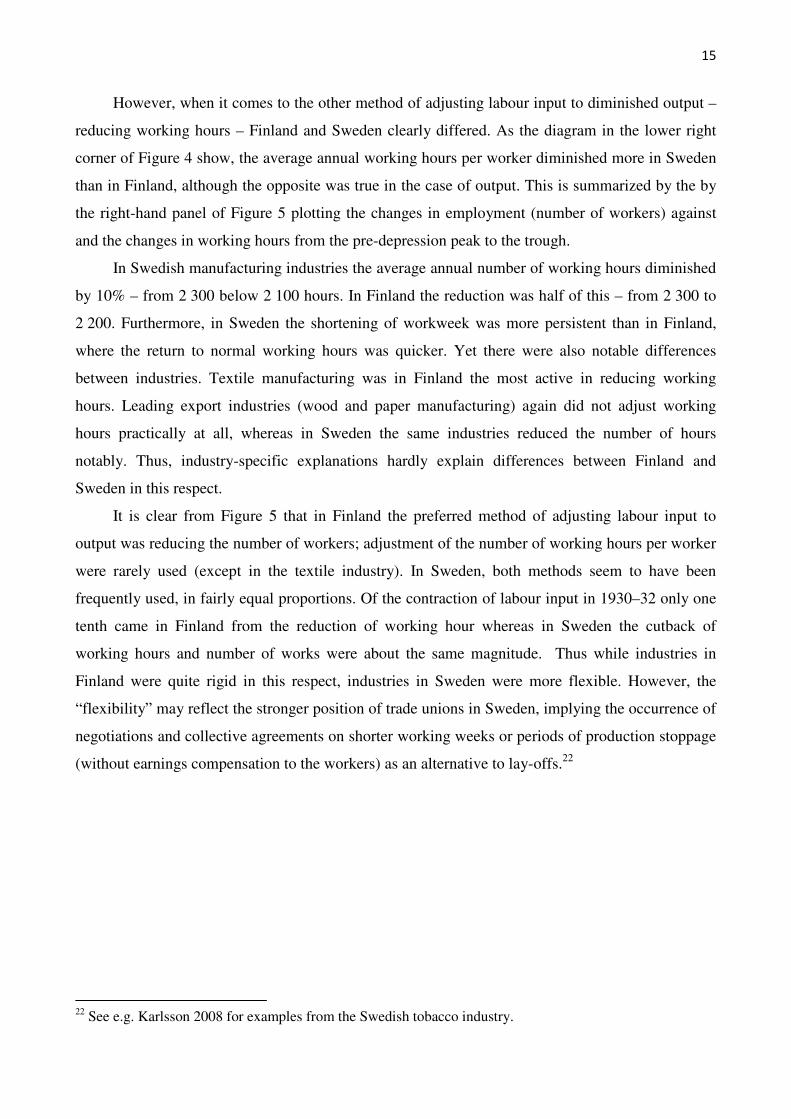
However, when it comes to the other method of adjusting labour input to diminished output –
reducing working hours – Finland and Sweden clearly differed. As the diagram in the lower right
corner of Figure 4 show, the average annual working hours per worker diminished more in Sweden
than in Finland, although the opposite was true in the case of output. This is summarized by the by
the right-hand panel of Figure 5 plotting the changes in employment (number of workers) against
and the changes in working hours from the pre-depression peak to the trough.
In Swedish manufacturing industries the average annual number of working hours diminished
by 10% – from 2 300 below 2 100 hours. In Finland the reduction was half of this – from 2 300 to
2 200. Furthermore, in Sweden the shortening of workweek was more persistent than in Finland,
where the return to normal working hours was quicker. Yet there were also notable differences
between industries. Textile manufacturing was in Finland the most active in reducing working
hours. Leading export industries (wood and paper manufacturing) again did not adjust working
hours practically at all, whereas in Sweden the same industries reduced the number of hours
notably. Thus, industry-specific explanations hardly explain differences between Finland and
Sweden in this respect.
It is clear from Figure 5 that in Finland the preferred method of adjusting labour input to
output was reducing the number of workers; adjustment of the number of working hours per worker
were rarely used (except in the textile industry). In Sweden, both methods seem to have been
frequently used, in fairly equal proportions. Of the contraction of labour input in 1930–32 only one
tenth came in Finland from the reduction of working hour whereas in Sweden the cutback of
working hours and number of works were about the same magnitude. Thus while industries in
Finland were quite rigid in this respect, industries in Sweden were more flexible. However, the
“flexibility” may reflect the stronger position of trade unions in Sweden, implying the occurrence of
negotiations and collective agreements on shorter working weeks or periods of production stoppage
(without earnings compensation to the workers) as an alternative to lay-offs.22
22 See e.g. Karlsson 2008 for examples from the Swedish tobacco industry.
16
Figure 4. Average annual working hours in five major manufacturing industries in Finland and Sweden, 1926–1938
1800
1900
2000
2100
2200
2300
2400
2500
2600
1926 1928 1930 1932 1934 1936 1938
Food
Sweden Finland
1800
1900
2000
2100
2200
2300
2400
2500
2600
1926 1928 1930 1932 1934 1936 1938
Textile
Sweden Finland
1800
1900
2000
2100
2200
2300
2400
2500
2600
1926 1928 1930 1932 1934 1936 1938
Wood
Sweden Finland
1800
1900
2000
2100
2200
2300
2400
2500
2600
1926 1928 1930 1932 1934 1936 1938
Paper
Sweden Finland
1800
1900
2000
2100
2200
2300
2400
2500
2600
1926 1928 1930 1932 1934 1936 1938
Metal
Sweden Finland
1800
1900
2000
2100
2200
2300
2400
2500
2600
1926 1928 1930 1932 1934 1936 1938
ALL 5 INDUSTRIES
Finland Sweden
17
Figure 5. Output, employment and average working hours per worker in six major manufacturing industries in Finland and Sweden during the Great Depression, trough-to-peak
Note * Output of Finnish paper industry grew also
during the depression years, i.e. trough/peak
ratio was actually above 1.
Note There is no data on working hours in
manufacturing of non-metallic mineral products
in Sweden.
Note: Peak and trough years are variable specific.
6. Nominal wages
The nominal wage indices we have constructed describe the actual total hourly wages or earnings –
not wage rates, not wages paid by hour, not wages for “normal work time” but including also the
pay for overtime. The Swedish nominal wage indices have been calculated as weighted averages of
indices for male, female and under-aged workers. Finnish indices are calculated, always when
possible, as weighted average of men’s and women’s wages.23
23 There is almost no data on wages for under-aged workers, but in Finland their share was much smaller than in Sweden.
METAL
MINERAL
TEXTILE
PAPER
WOOD
FOOD
Metal
Mineral
Textile
Paper*
Wood
Food
0,5
0,6
0,7
0,8
0,9
1
0,5 0,6 0,7 0,8 0,9 1,0
Nu
mb
er
of
wo
rke
rs
Output
Employment and output
Sweden Finland
METAL
TEXTILE
PAPER
WOOD
FOOD
Metal
Mineral
Textile
Paper
Wood
Food
0,5
0,6
0,7
0,8
0,9
1
0,5 0,6 0,7 0,8 0,9 1,0
Nu
mb
er
of
wo
rke
rs
Hours per worker
Employment and working hours
Sweden Finland
18
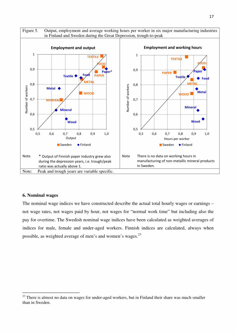
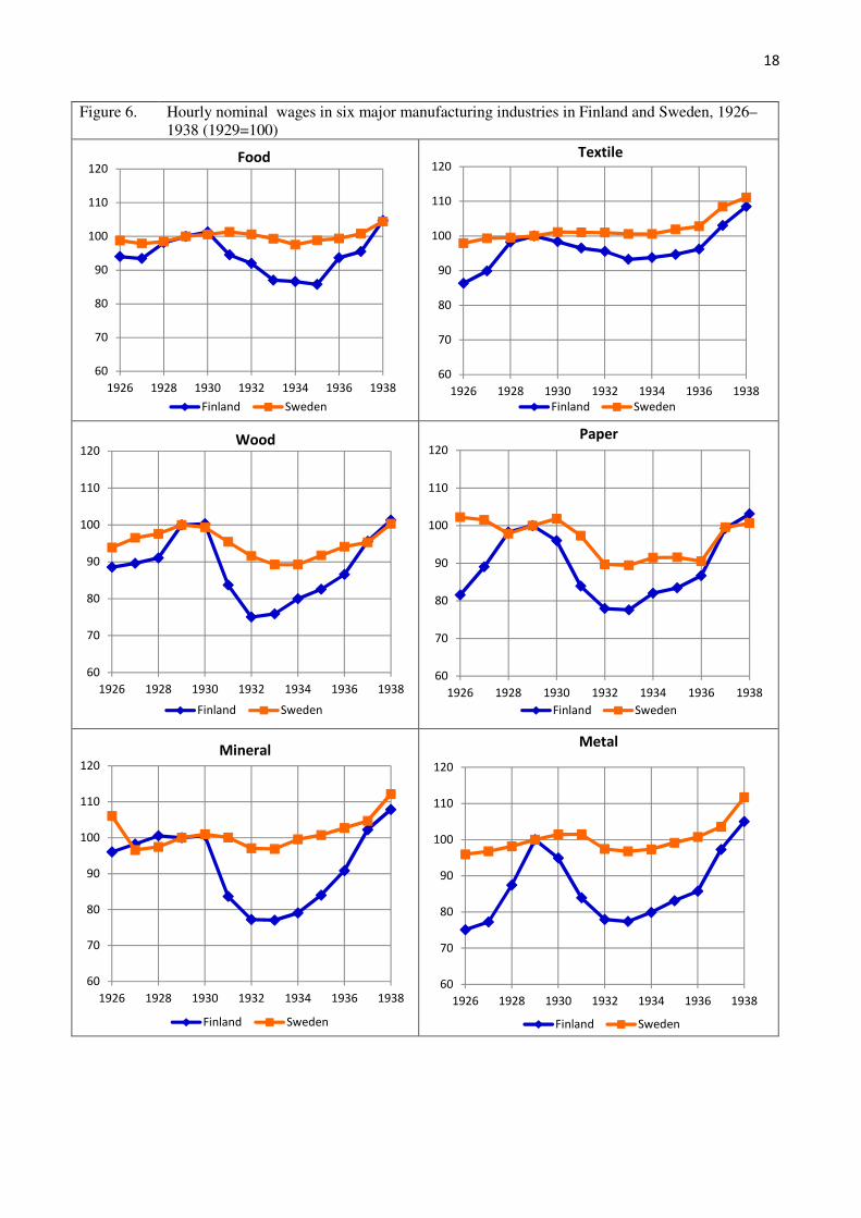
Figure 6. Hourly nominal wages in six major manufacturing industries in Finland and Sweden, 1926–1938 (1929=100)
60
70
80
90
100
110
120
1926 1928 1930 1932 1934 1936 1938
Food
Finland Sweden
60
70
80
90
100
110
120
1926 1928 1930 1932 1934 1936 1938
Textile
Finland Sweden
60
70
80
90
100
110
120
1926 1928 1930 1932 1934 1936 1938
Wood
Finland Sweden
60
70
80
90
100
110
120
1926 1928 1930 1932 1934 1936 1938
Paper
Finland Sweden
60
70
80
90
100
110
120
1926 1928 1930 1932 1934 1936 1938
Mineral
Finland Sweden
60
70
80
90
100
110
120
1926 1928 1930 1932 1934 1936 1938
Metal
Finland Sweden
19
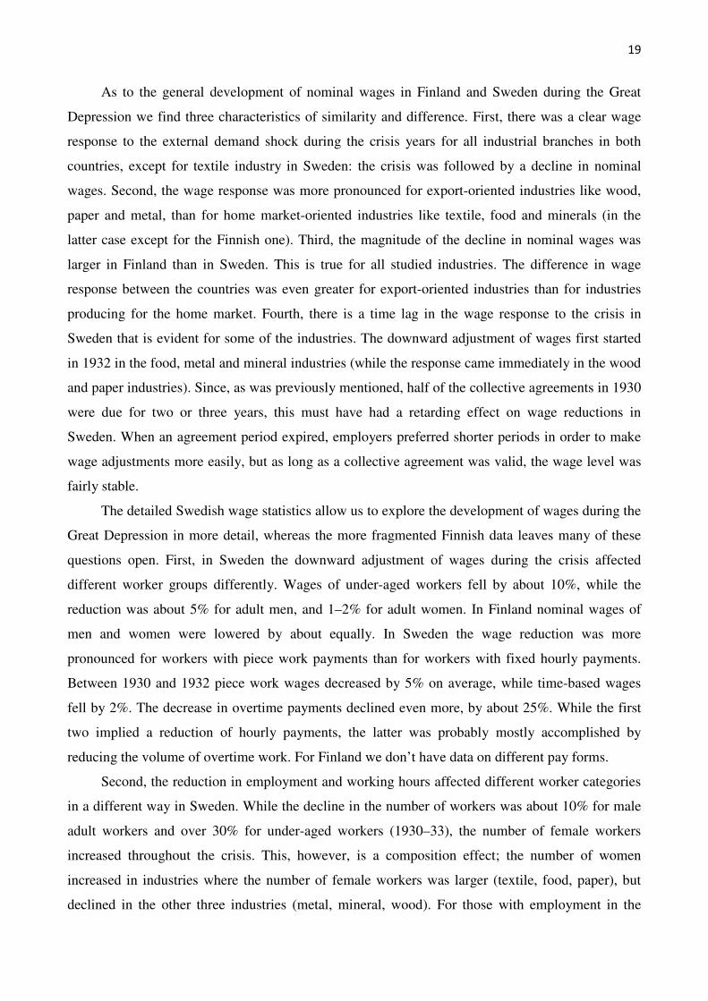
As to the general development of nominal wages in Finland and Sweden during the Great
Depression we find three characteristics of similarity and difference. First, there was a clear wage
response to the external demand shock during the crisis years for all industrial branches in both
countries, except for textile industry in Sweden: the crisis was followed by a decline in nominal
wages. Second, the wage response was more pronounced for export-oriented industries like wood,
paper and metal, than for home market-oriented industries like textile, food and minerals (in the
latter case except for the Finnish one). Third, the magnitude of the decline in nominal wages was
larger in Finland than in Sweden. This is true for all studied industries. The difference in wage
response between the countries was even greater for export-oriented industries than for industries
producing for the home market. Fourth, there is a time lag in the wage response to the crisis in
Sweden that is evident for some of the industries. The downward adjustment of wages first started
in 1932 in the food, metal and mineral industries (while the response came immediately in the wood
and paper industries). Since, as was previously mentioned, half of the collective agreements in 1930
were due for two or three years, this must have had a retarding effect on wage reductions in
Sweden. When an agreement period expired, employers preferred shorter periods in order to make
wage adjustments more easily, but as long as a collective agreement was valid, the wage level was
fairly stable.
The detailed Swedish wage statistics allow us to explore the development of wages during the
Great Depression in more detail, whereas the more fragmented Finnish data leaves many of these
questions open. First, in Sweden the downward adjustment of wages during the crisis affected
different worker groups differently. Wages of under-aged workers fell by about 10%, while the
reduction was about 5% for adult men, and 1–2% for adult women. In Finland nominal wages of
men and women were lowered by about equally. In Sweden the wage reduction was more
pronounced for workers with piece work payments than for workers with fixed hourly payments.
Between 1930 and 1932 piece work wages decreased by 5% on average, while time-based wages
fell by 2%. The decrease in overtime payments declined even more, by about 25%. While the first
two implied a reduction of hourly payments, the latter was probably mostly accomplished by
reducing the volume of overtime work. For Finland we don’t have data on different pay forms.
Second, the reduction in employment and working hours affected different worker categories
in a different way in Sweden. While the decline in the number of workers was about 10% for male
adult workers and over 30% for under-aged workers (1930–33), the number of female workers
increased throughout the crisis. This, however, is a composition effect; the number of women
increased in industries where the number of female workers was larger (textile, food, paper), but
declined in the other three industries (metal, mineral, wood). For those with employment in the
20
manufacturing industry, the number of working hours per worker and year diminished by 11% for
male workers, 6% for under-aged workers, and 3% for female workers in 1929–1932. This may
reflect the decline in overtime work and experiments with shorter working weeks or periods of non-
production during the crisis years. The proportion of working hours at piece work payment peaked
in 1929, and then fell with about 10% in two, three years (from 59% in 1929 to 54% in 1932).
Thus it seems that the manufacturing labour market in Sweden was to a large extent
segmented by gender, so that male and female workers did not compete over employment and
payments. For the male labour market, it could be assumed that the crisis induced selectivity in
employment and payments. In order to reduce wage costs, employers chose to lay off unskilled
workers (under-aged helpers, workers receiving piece work payments) and keep the skilled ones
(adult with fixed hourly wages). Also it could be assumed that under-aged workers had a weaker
position and could more easily be subject to wage cuts and lay-offs. The situation was in Finland
different in the respect that the share of women in manufacturing labour forces was double (38%)
that of Sweden (19%), whereas the share of under-aged workers was smaller (5% and 9%
respectively). So the share of adult male worker was in Finland clearly smaller (57%) than in
Sweden (72%).24
7. Real wages
While money wages are the same from both workers’ and employers’ point of view the real wages
are not. For workers it is the consumption real wage, i.e. nominal wages deflated with consumption
prices, that matters, whereas from employers’ point of view the key variable is the real product
wage, i.e. nominal wage divided by output price.25 In the following we examine the development of
both kinds of real wages. Real consumption wages have been calculated by deflating nominal prices
with consumer price indices.26
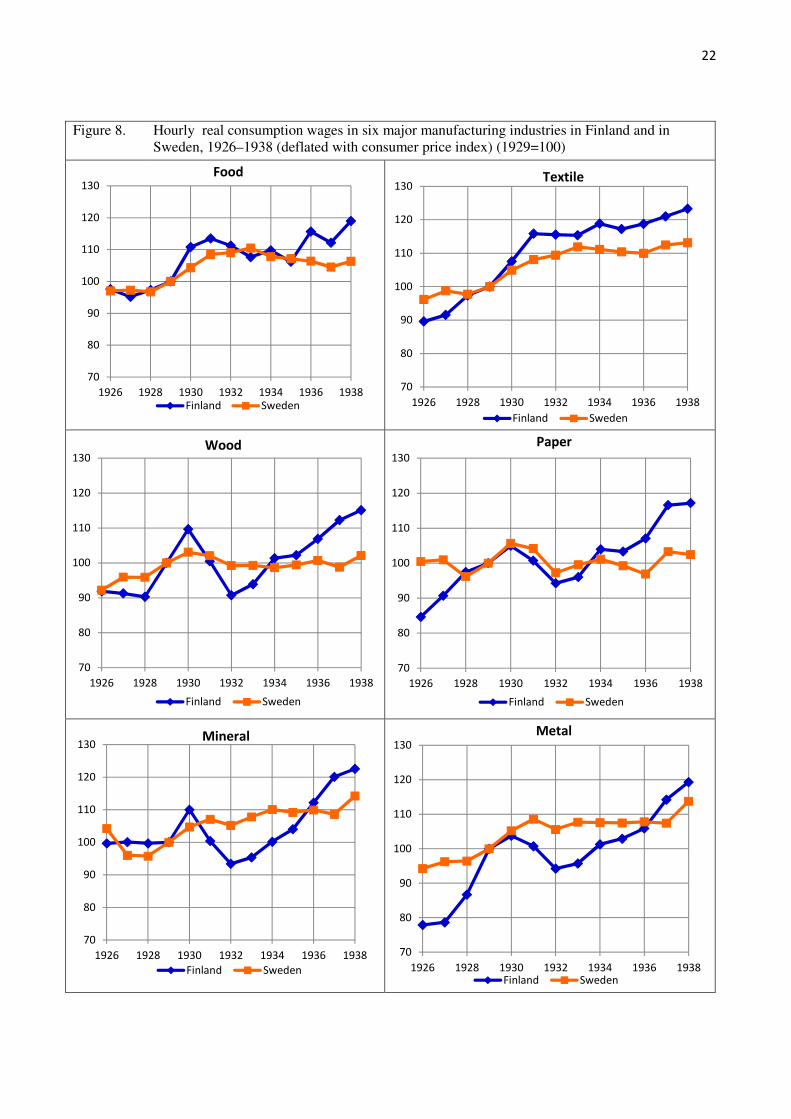
Figure 8 displays the development of real consumption wages in Finland and Sweden. Since
both wages and consumer prices were pressed down during the Great Depression, the real wage
pattern differs somewhat from the pattern of nominal wages; but still we find clear similarities. For
instance, we find signs of real wage reduction in almost all industries across countries, and the wage
response was more pronounced in industries that were export-oriented. However, the difference
24 All manufacturing averages in 1926–38 (averages of annual percentages). 25 See e.g. Backhouse 1991, p. 121. 26 The official Finnish consumer price index basket included direct taxes, weheres in Sweden there were indices with or without taxes. We have used indices without taxes, i.e. the Finnish index has been recalculated leaving out taxes.
21
between Finland and Sweden in the magnitude of wage response becomes smaller as measured as
consumption wages (compared to nominal wages), but the difference tend to remain.
Thus, there is a clear downward adjustment of real wages for five industries in Finland: food,
wood, paper, mineral and metal industries. In the textile industry real wages declined somewhat
between 1931 and 1933, but were more or less stable. As to the Swedish manufacturing we find a
much weaker wage reduction of real wages for most of the industries. Only in the paper industry
real wages were reduced to the same extent that in Finland.
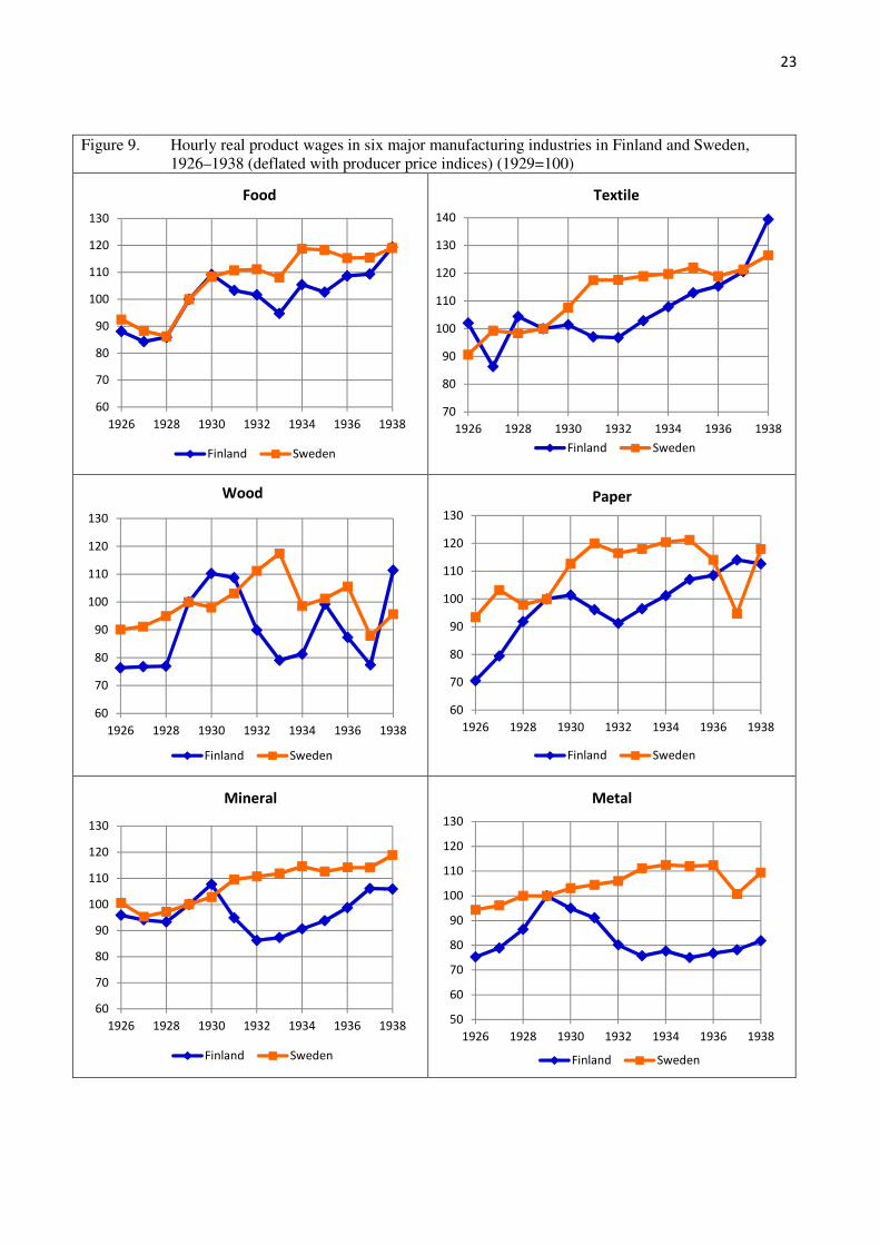
While real consumption wages indicate the standard of living of manufacturing workers in
different industries, real product wages indicate the relative cost of labour (compared the product
prices) for enterprises in the specific industries. Figure 9 displays the real product wages in the
studied six industries in Finland and Sweden. The main impression from comparing real
consumption wages remains and is even strengthened: Downward real wage adjustment as a
response to the economic crisis was made in Finland but hardly in Sweden. In three Finnish
manufacturing industries real product wages declined by 20–30% (wood, mineral, metal), and in
two by 10–15% (food, paper); the decline started immediately after the outbreak of the economic
crisis. There is no equivalent to this in the Swedish case. In four of the industries (food, textile,
mineral, metal) real product wages tended to increase throughout the crisis years. Only in the wood
and paper industries real product wages were reduced, but it happened long after the outbreak of the
economic crises. In the wood industry real product wages were subject to downward adjustment in
1933–37, and in the paper industry there was a very weak adjustment in 1931 and a more
pronounced starting in 1936. As was previously mentioned, it could be hypothesized that the lag in
the Swedish response was due to binding collective agreement that prevented employers to enforce
a more rapid response the necessity to cut labour costs.
22
Figure 8. Hourly real consumption wages in six major manufacturing industries in Finland and in Sweden, 1926–1938 (deflated with consumer price index) (1929=100)
70
80
90
100
110
120
130
1926 1928 1930 1932 1934 1936 1938
Food
Finland Sweden
70
80
90
100
110
120
130
1926 1928 1930 1932 1934 1936 1938
Textile
Finland Sweden
70
80
90
100
110
120
130
1926 1928 1930 1932 1934 1936 1938
Wood
Finland Sweden
70
80
90
100
110
120
130
1926 1928 1930 1932 1934 1936 1938
Paper
Finland Sweden
70
80
90
100
110
120
130
1926 1928 1930 1932 1934 1936 1938
Mineral
Finland Sweden
70
80
90
100
110
120
130
1926 1928 1930 1932 1934 1936 1938
Metal
Finland Sweden
23
Figure 9. Hourly real product wages in six major manufacturing industries in Finland and Sweden, 1926–1938 (deflated with producer price indices) (1929=100)
60
70
80
90
100
110
120
130
1926 1928 1930 1932 1934 1936 1938
Food
Finland Sweden
70
80
90
100
110
120
130
140
1926 1928 1930 1932 1934 1936 1938
Textile
Finland Sweden
60
70
80
90
100
110
120
130
1926 1928 1930 1932 1934 1936 1938
Wood
Finland Sweden
60
70
80
90
100
110
120
130
1926 1928 1930 1932 1934 1936 1938
Paper
Finland Sweden
60
70
80
90
100
110
120
130
1926 1928 1930 1932 1934 1936 1938
Mineral
Finland Sweden
50
60
70
80
90
100
110
120
130
1926 1928 1930 1932 1934 1936 1938
Metal
Finland Sweden
24
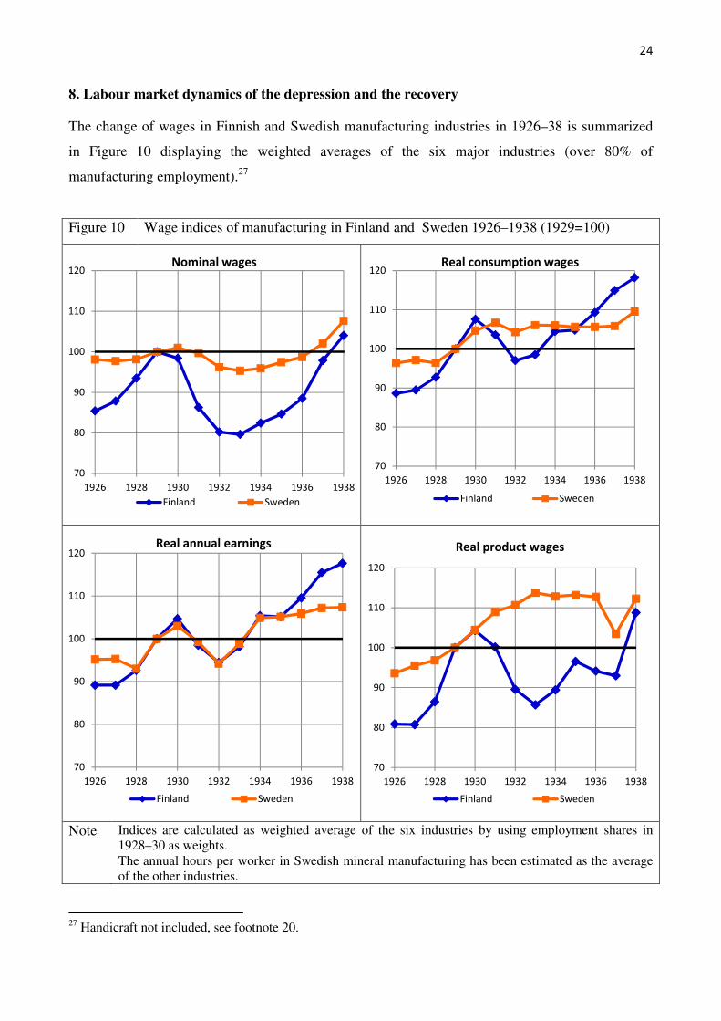
8. Labour market dynamics of the depression and the recovery
The change of wages in Finnish and Swedish manufacturing industries in 1926–38 is summarized
in Figure 10 displaying the weighted averages of the six major industries (over 80% of
manufacturing employment).27
Figure 10 Wage indices of manufacturing in Finland and Sweden 1926–1938 (1929=100)
Note Indices are calculated as weighted average of the six industries by using employment shares in 1928–30 as weights. The annual hours per worker in Swedish mineral manufacturing has been estimated as the average of the other industries.
27 Handicraft not included, see footnote 20.
70
80
90
100
110
120
1926 1928 1930 1932 1934 1936 1938
Nominal wages
Finland Sweden
70
80
90
100
110
120
1926 1928 1930 1932 1934 1936 1938
Real consumption wages
Finland Sweden
70
80
90
100
110
120
1926 1928 1930 1932 1934 1936 1938
Real annual earnings
Finland Sweden
70
80
90
100
110
120
1926 1928 1930 1932 1934 1936 1938
Real product wages
Finland Sweden
25
Nominal wages fell dramatically in Finland during the depression (20% on average), whereas
in Sweden money wages were quite rigid (falling by 5%). In Sweden nominal inertia was greater
for wages than for consumer prices resulting in rising real consumption wages in the depression.
Also in Finland real consumption wages were counter-cyclical in the beginning of the depression
(1930) but in the trough they went slightly below the pre-depression level. Thus, prices were less
sticky in relation to consumer price in Finland than in Sweden. Compared to the wage level in 1929,
hourly real consumption wages were in Sweden notably higher than in Finland during the
depression but in the recovery Finnish real wages caught up and passed by in 1936–38. And if we
take into account also the changes in working hours and estimate real annual earnings Finnish and
Swedish curves practically merge in the depression and the beginning of the recovery (1928–35),
but also this variable indicates more favourable development for Finnish than for Swedish workers.
However, part of this is, of course, to be explained by the fact that that Finnish manufacturing
workers toiled more than their Swedish brothers and sisters.
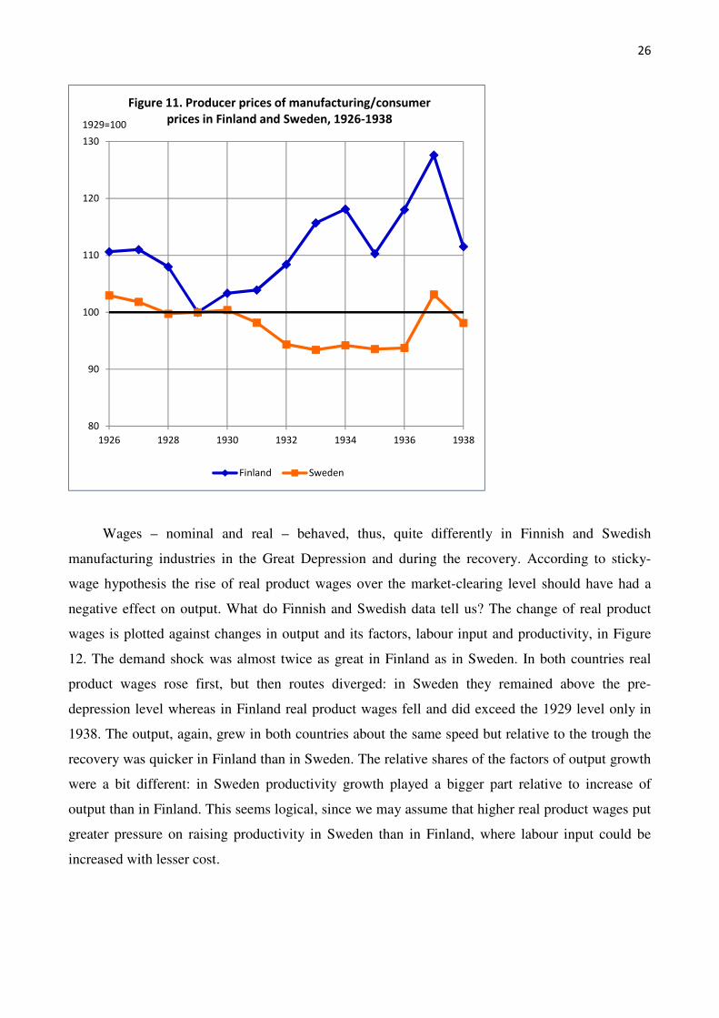
When we change the point of view from workers’ living standard, i.e. from real consumption
wages to real product wages relevant for labour demand the differences between Finland and
Sweden become much greater. In Sweden real product wages rose in 1933 by 14% above the 1929
level, whereas in Finland they were below that level by equal amount! In Sweden real product
wages were as clearly counter-cyclical as they were pro-cyclical in Finland. This was result of two
factors: first, the greater flexibility of Finnish nominal wages, and second, different development of
producer prices to consumer prices. In Finland product prices of manufacturing rose notably in
relation to consumer prices, whereas in Sweden they declined (until 1936) (se Figure 11). This
“price wedge” made the adjustment of the labour market of manufacturing easier in Finland than in
Sweden, since the profitability of firms and real earnings of workers could increase simultaneously.
26
Wages – nominal and real – behaved, thus, quite differently in Finnish and Swedish
manufacturing industries in the Great Depression and during the recovery. According to sticky-
wage hypothesis the rise of real product wages over the market-clearing level should have had a
negative effect on output. What do Finnish and Swedish data tell us? The change of real product
wages is plotted against changes in output and its factors, labour input and productivity, in Figure
12. The demand shock was almost twice as great in Finland as in Sweden. In both countries real
product wages rose first, but then routes diverged: in Sweden they remained above the pre-
depression level whereas in Finland real product wages fell and did exceed the 1929 level only in
1938. The output, again, grew in both countries about the same speed but relative to the trough the
recovery was quicker in Finland than in Sweden. The relative shares of the factors of output growth
were a bit different: in Sweden productivity growth played a bigger part relative to increase of
output than in Finland. This seems logical, since we may assume that higher real product wages put
greater pressure on raising productivity in Sweden than in Finland, where labour input could be
increased with lesser cost.
80
90
100
110
120
130
1926 1928 1930 1932 1934 1936 1938
1929=100
Figure 11. Producer prices of manufacturing/consumer
prices in Finland and Sweden, 1926-1938
Finland Sweden
27
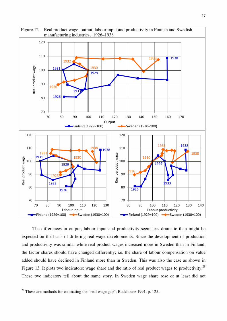
Figure 12. Real product wage, output, labour input and productivity in Finnish and Swedish manufacturing industries, 1926–1938
The differences in output, labour input and productivity seem less dramatic than might be
expected on the basis of differing real-wage developments. Since the development of production
and productivity was similar while real product wages increased more in Sweden than in Finland,
the factor shares should have changed differently; i.e. the share of labour compensation on value
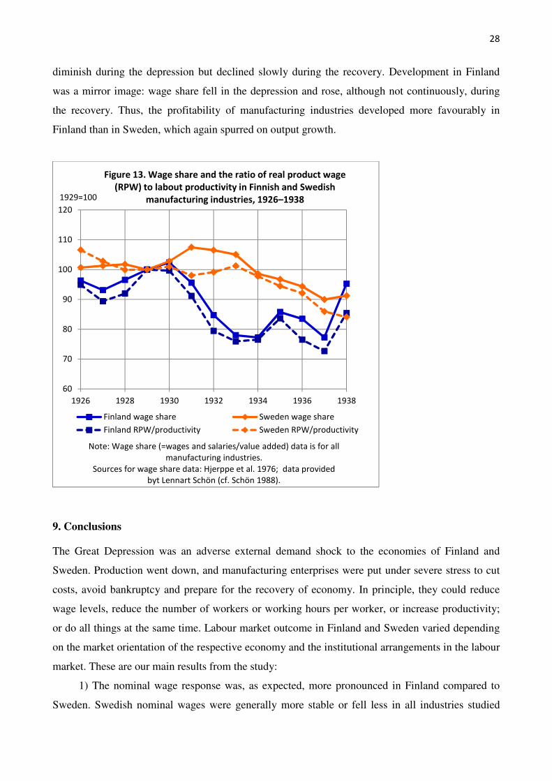
added should have declined in Finland more than in Sweden. This was also the case as shown in
Figure 13. It plots two indicators: wage share and the ratio of real product wages to productivity.28
These two indicators tell about the same story. In Sweden wage share rose or at least did not
28 These are methods for estimating the “real wage gap”; Backhouse 1991, p. 125.
1926
1929
1931
1933
1938
1926
1930
19321938
70
80
90
100
110
120
70 80 90 100 110 120 130 140 150 160 170
Re
al
pro
du
ct w
ag
e
OutputFinland (1929=100) Sweden (1930=100)
1926
1929
1931
1933
1938
1926
19301932
1938
70
80
90
100
110
120
70 80 90 100 110 120 130
Re
al
pro
du
ct w
ag
e
Labour input
Finland (1929=100) Sweden (1930=100)
1926
1929
1933
1938
1926
1930
1933
1938
70
80
90
100
110
120
80 90 100 110 120 130 140
Re
al
pe
rod
uct
wa
ge
Labour productivity
Finland (1929=100) Sweden (1930=100)
28
diminish during the depression but declined slowly during the recovery. Development in Finland
was a mirror image: wage share fell in the depression and rose, although not continuously, during
the recovery. Thus, the profitability of manufacturing industries developed more favourably in
Finland than in Sweden, which again spurred on output growth.
9. Conclusions
The Great Depression was an adverse external demand shock to the economies of Finland and
Sweden. Production went down, and manufacturing enterprises were put under severe stress to cut
costs, avoid bankruptcy and prepare for the recovery of economy. In principle, they could reduce
wage levels, reduce the number of workers or working hours per worker, or increase productivity;
or do all things at the same time. Labour market outcome in Finland and Sweden varied depending
on the market orientation of the respective economy and the institutional arrangements in the labour
market. These are our main results from the study:
1) The nominal wage response was, as expected, more pronounced in Finland compared to
Sweden. Swedish nominal wages were generally more stable or fell less in all industries studied
60
70
80
90
100
110
120
1926 1928 1930 1932 1934 1936 1938
1929=100
Note: Wage share (=wages and salaries/value added) data is for all
manufacturing industries.
Sources for wage share data: Hjerppe et al. 1976; data provided
byt Lennart Schön (cf. Schön 1988).
Figure 13. Wage share and the ratio of real product wage
(RPW) to labout productivity in Finnish and Swedish
manufacturing industries, 1926–1938
Finland wage share Sweden wage share
Finland RPW/productivity Sweden RPW/productivity
29
than the corresponding nominal wages in Finland. As to the real wage response, results confirm the
above mentioned basic difference between Finnish and Swedish economies. While we find no real
wage response to external shock in Sweden except for the paper industry, real wages decreased for
all studied Finnish industries. Our results thus support the overall hypothesis that wages in Sweden
were stickier due to higher union density, larger collective agreement coverage and better
unemployment insurances.
2) The wage response varied across industries depending on the market orientation of the
industry in question, and in a similar way in Finland and Sweden. Wage reductions were greater in
export-oriented industries while it was less in industries producing for the home market; two
Swedish home market-oriented industries (food, textile) experienced no reduction in wages at all.
3) Results indicate that labour productivity in the manufacturing industry of Finland and
Sweden stagnated during the Great Depression and increased on average after the depression.
Differences between countries were minor relative to remarkably different development of real
product wages. Consequently the share of wages on value added declined more rapidly in Finland
than in Sweden.
4) We hypothesized the employment response to be of greater importance in Sweden than in
Finland because we expected wages to be stickier in Sweden. An alternative way of reducing wage
costs when wage cuts were not possible because of institutional reasons was reducing the number of
workers or the number of working hours per worker. Our results indicate that in both Finland and
Sweden the number of workers was reduced in step with the declining production output, although
the variation across industrial branches was greater in Finland. With regards to the choice between
the reduction of the number of workers or the number of working hours per worker, results indicate
that manufacturing industries in Sweden were flexible on both dimensions while the Finnish
industries were more prone to cut the number of workers but rarely elaborated on the number of
working hours.
5) The comparison of Finnish and Swedish manufacturing industries supports the conclusion
of Hatton and Thomas that the recovery from a macroeconomic shock “is conditioned both by the
scale of the shock and by the structure of labour market institutions”29 Yet our results also point out
that the economic outcomes during and after depression do not straightforwardly depend on
flexibility or stickiness of wages.
29 Hatton & Thomas 2013, p. 351.
30
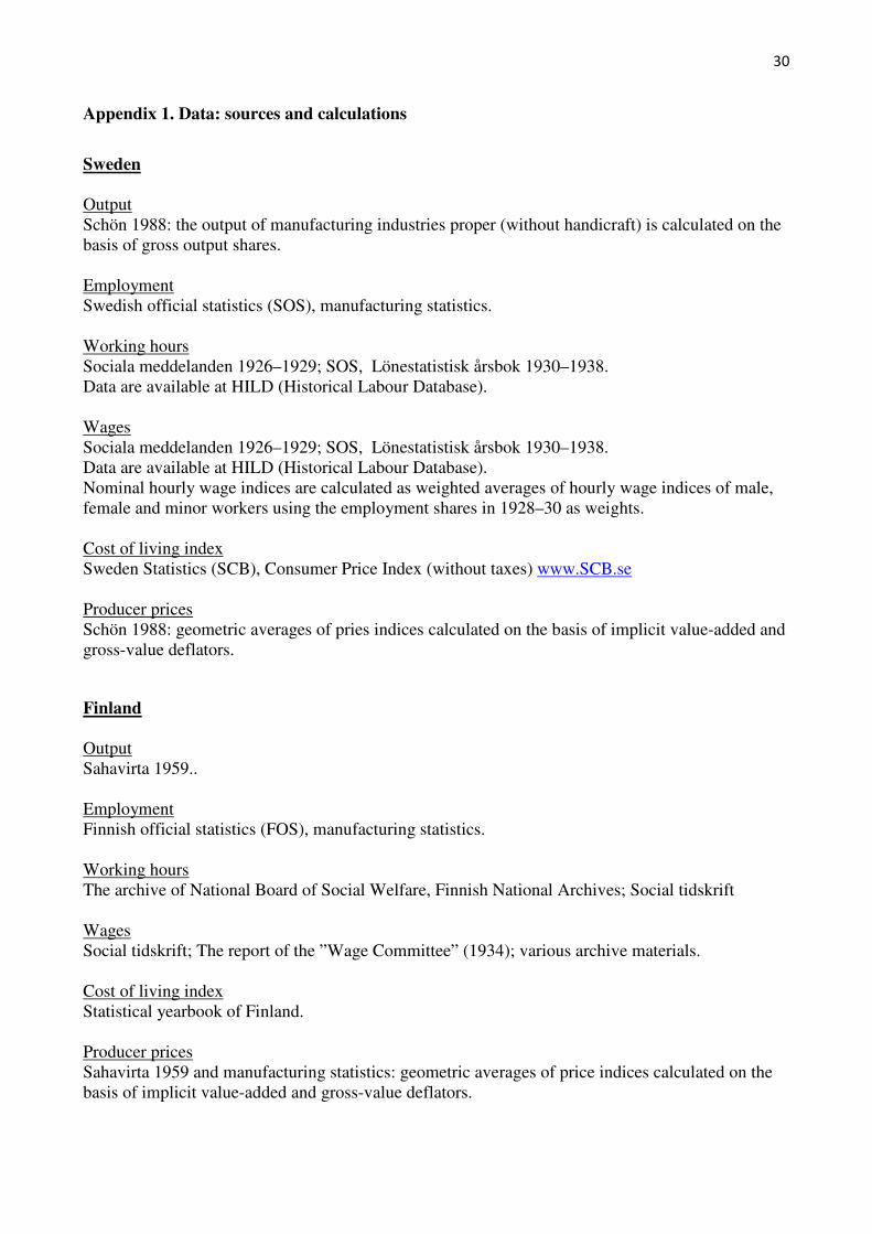
Appendix 1. Data: sources and calculations
Sweden Output Schön 1988: the output of manufacturing industries proper (without handicraft) is calculated on the basis of gross output shares. Employment Swedish official statistics (SOS), manufacturing statistics. Working hours Sociala meddelanden 1926–1929; SOS, Lönestatistisk årsbok 1930–1938. Data are available at HILD (Historical Labour Database). Wages Sociala meddelanden 1926–1929; SOS, Lönestatistisk årsbok 1930–1938. Data are available at HILD (Historical Labour Database). Nominal hourly wage indices are calculated as weighted averages of hourly wage indices of male, female and minor workers using the employment shares in 1928–30 as weights. Cost of living index Sweden Statistics (SCB), Consumer Price Index (without taxes) www.SCB.se Producer prices Schön 1988: geometric averages of pries indices calculated on the basis of implicit value-added and gross-value deflators.
Finland Output Sahavirta 1959.. Employment Finnish official statistics (FOS), manufacturing statistics. Working hours The archive of National Board of Social Welfare, Finnish National Archives; Social tidskrift Wages Social tidskrift; The report of the ”Wage Committee” (1934); various archive materials. Cost of living index Statistical yearbook of Finland. Producer prices Sahavirta 1959 and manufacturing statistics: geometric averages of price indices calculated on the basis of implicit value-added and gross-value deflators.
31
References
Ala-Kapee & Valkonen (1982): Yhdessä elämä turvalliseksi. SAK I. SAK-laisen
ammattiyhdistysliikkeen kehitys vuoteen 1930, Helsinki: SAK. Backhouse, Roger (1991): Applied United Kingdom Macroeconomics, Wiley-Blackwell. Bergolm, Tapio (2003): A Short History of SAK – the Cnetral Organisation of Finnish Trade
Unions. Valkeala: Painokarelia. Bernanke, Ben S. (1986): ‘Employment, Hours and Earnings in the Depression: An Analysis of
Eight Manufacturing Industries’, The American Economic Review, 76, 82–109. Bernanke, Ben S. (1995): ‘The Macroeconomics of the Great Depression: A Comparative
Approach’, Journal of Money, Credit and Banking, 27, 1–28. Bernanke, Ben S. & Harold James (2000 [1991]): ‘The gold standard, deflation and financial crisis
in the Great Depression: an international comparison’, in Ben S. Bernanke: Essays on the Great
Depression, Princeton: Princeton University Press, 70–107 Bernanke, Ben S. & Kevin Carey (1996): ‘Nominal Wage Stickiness and Aggregate Supply in the
Great Depression’, The Quarterly Journal of Economics, 111, 853–883. Bordo, Michael D. & Christopher J. Erceg & Charles L. Evans (2000): ‘Money, Sticky Wages, and
the Great Depression’, The American Economic Review, 90, 1447–63 Dimsdale, N. H., Nickell, S. J., & Horsewood, N. (1989): ‘Real Wages and Unemployment in
Britain during the 1930s’, Economic Journal, 99, 271–92. Eichengreen, Barry & Jeffrey Sachs (1985): ‘Exchange rates and recovery in the 1930s’, Journal of
Economic History, 44, 925–46. Fregert, Klas (2000): ‘The Great Depression in Sweden as a wage coordination failure’, European
Review of Economic History, 4, 341–60. Göransson, Håkan (1988), Kollektivavtalet som fredspliktsinstrument. De grundläggande förbuden
mot stridsåtgärder i historisk och internationell belysning. Stockholm: Juristförlaget. Hjerppe, Reino et al. (1976): Suomen teollisuus ja teollinen käsityö 1900–1965 [Industry and
Industrial Handicraft in Finland 1900–1965], Helsinki: Suomen Pankki. Hjerppe, Riitta (1989): The Finnish Economy 1860-1985. Growth and Structural Change, Helsinki:
Bank of Finland. Karlsson, Tobias. Downsizing: personnel reductions at the Swedish Tobacco Monopoly, 1915-1939.
Lund, 2008. Kettunen, Pauli (1986): Poliittinen liike ja sosiaalinen kollektiivisuus. Tutkimus
sosialidemokratiasta ja ammattiyhdistysliikkeestä Suomessa 1918-1930, Helsinki : Suomen historiallinen seura.
Kettunen, Pauli (1990): ‘Hur legitimerades arbetsgivarnas politik i “första republikens” Finland?’ in Industriell demokrati i Norden ed. by Daniel Fleming, Lund: Arkiv förlag, 129–90.
Knoellinger, Carl Erik (1960): Labor in Finland, Camridge (Mass): Harvard University Press Lundh, Christer (2008): Arbetsmarknadens karteller. Nya perspektiv på det svenska
kollektivavtalssystemets historia. Stockholm: Norstedts Akademiska Förlag. Lundh, Christer (2010): Spelets regler. Institutioner och lönebildningen på den svenska
arbetsmarknaden, 2. upplagan, Stockholm: SNS. Madsen, Jakob B. (2004): Price and wage stickiness during the Great Depression, European Review
of Economic History, 263–295. Mansner, Markku (1981): Suomalaista yhteiskuntaa rakentamassa. Suomen Työnantajain
Keskusliitto 1907–1940, Jyväskylä. Sahavirta, Margit (1959): Teollisuustuotannon volyymi-indeksi vuosina 1925–1958,
Tilastokatsauksia 1959:10, 39–46. Schön, Lennart (1988): Historiska nationalräkenskaperna för Sverige. Industri och hantverk 1800–
1980 Lund: Ekonomisk-historiska föreningen I Lund.

32
Schön, Lennart (1998): ‘Industrial crises in a model of long cycles. Sweden in an international perspective’, Economic crises and restructuring in history ed. by Timo Myllyntaus, St Katharinen: Scripta Mercature Verlag, 397–413.
Schön, Lennart & Olle Krantz (2012): Swedish Historical National Accounts 1560–2010.
http://www.ekh.lu.se/en/research/shna1560-2010 Valkonen, Marjaana (1987): Yhdessä elämä turvalliseksi. SAK II. Suomen Ammattiyhdistysten
Keskusliitto 1930–1947, Helsinki: SAK.