STOCHASTIC BLOCK MIRROR DESCENT METHODS FORNONSMOOTH AND STOCHASTIC OPTIMIZATION ∗

CONG D. DANG † AND GUANGHUI LAN ‡

Abstract. In this paper, we present a new stochastic algorithm, namely the stochastic block mirror descent (SBMD) methodfor solving large-scale nonsmooth and stochastic optimization problems. The basic idea of this algorithm is to incorporate theblock-coordinate decomposition and an incremental block averaging scheme into the classic (stochastic) mirror-descent method,in order to significantly reduce the cost per iteration of the latter algorithm. We establish the rate of convergence of the SBMDmethod along with its associated large-deviation results for solving general nonsmooth and stochastic optimizaiton problems. Wealso introduce different variants of this method and establish their rate of convergence for solving strongly convex, smooth, andcomposite optimization problems, as well as certain nonconvex optimization problems. To the best of our knowledge, all thesedevelopments related to the SBMD methods are new in the stochastic optimization literature. Moreover, some of our results alsoseem to be new for block coordinate descent methods for deterministic optimization.

Keywords. Stochastic Optimization, Mirror Descent, Block Coordinate Descent, Nonsmooth Optimization, Stochastic Compos-ite Optimization, Metric Learning

AMS subject classifications. 62L20, 90C25, 90C15, 68Q25

1. Introduction. The basic problem of interest in the paper is the stochastic programming (SP) problemgiven by

f∗ := minx∈X{f(x) := E[F (x, ξ)]}. (1.1)

Here X ∈ Rn is a closed convex set, ξ is a random variable with support Ξ ⊆ Rd and F (·, ξ) : X → R iscontinuous for every ξ ∈ Ξ. In addition, we assume that X has a block structure, i.e.,

X = X1 ×X2 × · · · ×Xb, (1.2)

where Xi ⊆ Rni , i = 1, . . . , b, are closed convex sets with n1 + n2 + . . .+ nb = n.The last few years have seen a resurgence of interest in the block coordinate descent (BCD) method for

solving problems with X given in the form of (1.2). In comparision with regular first-order methods, eachiteration of these methods updates only one block of variables. In particular, if each block consists of onlyone variable (i.e., ni = 1, i = 1, . . . , b), then the BCD method becomes the simplest coordinate descent (CD)method. Although simple, these methods are found to be effective in solving huge-scale problems with n as bigas 108−1012 (see, e.g., [28, 19, 29, 33, 4]), and hence are very useful for dealing with high-dimensional problems,especially those from large-scale data analysis applications. While earlier studies on the BCD method werefocused on their asymptotical convergence behaviour (see, e.g., [22, 38] and also [39, 40]), much recent efforthas been directed to the complexity analysis of these types of methods (see [28, 19, 35, 33, 4]. In particular,Nesterov [28] was among the first (see also Leventhal and Lewis [19], and Shalev-Shwartz and Tewari [35]) toanalyze the iteration complexity of a randomized BCD method for minimizing smooth convex functions. Morerecently, the BCD methods were further enhanced by Richtarik and Takac [33], Beck and Tetruashvili [4], Luand Xiao [21], etc. We refer to [33] for an excellent review on the earlier developments of BCD methods.

However, to the best of our knowledge, most current BCD methods were designed for solving determinisitcoptimization problems. One possible approach for solving problem (1.1), based on existing BCD methods andthe sample average approximation (SAA) [36], can be described as follows. For a given set of i.i.d. samples

(dataset) ξk, k = 1, . . . , N , of ξ, we first approximate f(·) in (1.1) by f(x) := 1N

∑Nk=1 F (x, ξk) and then apply

the BCD methods to minx∈X f(x). Since ξk, k = 1, . . . , N , are fixed a priori, by recursively updating the(sub)gradient of f (see [28, 29]), the iteration cost of the BCD method can be considerably smaller than that

∗September, 2013. This research was partially supported by NSF grants CMMI-1000347, CMMI-1254446, DMS-1319050, andONR grant N00014-13-1-0036.†Department of Industrial and Systems Engineering, University of Florida, Gainesville, FL, 32611. (email: congdd@ufl.edu).‡Department of Industrial and Systems Engineering, University of Florida, Gainesville, FL, 32611. (email: glan@ise.ufl.edu).

1

of the gradient descent methods. However, the above SAA approach is also known for the following drawbacks:a) the high memory requirement to store ξk, k = 1, . . . , N ; b) the high dependence (at least linear) of theiteration cost on the sample size N , which can be expensive when dealing with large datasets; and c) thedifficulty to apply the approach to the on-line setting where one needs to update the solution whenever a newpiece of data ξk is collected.

A different approach to solve problem (1.1) is called stochastic approximation (SA), which was initiallyproposed by Robbins and Monro [34] in 1950s for solving strongly convex SP problems (see also [31, 32]). TheSA method has also attracted much interest recently (see, e.g., [24, 14, 30, 7, 8, 20, 9, 23, 10, 11, 13, 27, 41]).In particular, Nemirovski et. al. [24] presented a properly modified SA approach, namely, the mirror descentSA for solving general nonsmooth convex SP problems. Lan [14] introduced a unified optimal SA method forsmooth, nonsmooth and stochastic optimization (see also [7, 8] for a more general framework). Ghadimi andLan [9] presented novel SA methods for nonconvex optimization (see also [10]). Related methods, based ondual averaging, have been studied in [11, 13, 27, 41]. Note that all these SA algorithms only need to accessone single ξk at each iteration, and hence does not require much memory. In addition, their iteration costis independent of the sample size N . However, since these algorithms need to update the whole vector x ateach iteration, their iteration cost can strongly depend on n unless the problem is very sparse (see, e.g., [30]).In addition, it is unclear whether the SA methods can benefit from the recursive updating as in the BCDmethods, since the samples ξk used in different iterations are supposed to be independent.

Our main goal in this paper is to present a new class of stochastic methods, referered to as the stochasticblock mirror descent (SBMD) methods, by incorporating the aforementioned block-coordinate decompositioninto the classic (stochastic) mirror descent method ([25, 3, 24]). Our study has been mainly motivated bysolving an important class of SP problems with F (x, ξ) = ψ(Bx, ξ), where B is a certain linear operator andψ is a relatively simple function. These problems arise from many machine learning applications, where ψis a loss function and B denotes a certain basis (or dictionary) obtained by, e.g., metric learning (e.g., [42]).Each iteration of existing SA methods would require O(n2) arithmetic operations to compute Bx and becomesprohibitive if n exceeds 106. On the other hand, by using block-coordinate decomposition with ni = 1, theiteration cost of the SBMD algorithms can be significantly reduced to O(n), which can be further reduced ifB and ξk are sparse (see Subsection 2.1 for more discussions). Our development has also been motivated bythe situation when the bottleneck of the mirror descent method exists in the projection (or prox-mapping)subproblems (see (2.5)). In this case, we can also significantly reduce the iteration cost by using the block-coordinate decomposition, since each iteration of the SBMD method requires only one projection over Xi forsome 1 ≤ i ≤ b, while the mirror descent method needs to perform the projectons over Xi for all 1 ≤ i ≤ b.

Our contribution in this paper mainly lies in the following aspects. Firstly, we introduce the block de-compsition into the classic mirror descent method for solving general nonsmooth optimization problems. Eachiteration of this algorithm updates one block of the search point along a stochastic (sub)gradient Gik(xk, ξk).Here, the index ik is randomly chosen and G(x, ξ) is an unbiased estimator of the subgradient of f(·), i.e.,

E[G(x, ξ)] = g(x) ∈ ∂f(x), ∀x ∈ X. (1.3)

In addition, in order to compute the output of the algorithm, we introduce an incremental block averagingscheme, which updates only one block of the weighted sum of the search points in each iteration. We demon-strate that if f(·) is a general nonsmooth convex function, then the number of iterations performed by theSBMD method to find an ε-solution of (1.1), i.e., a point x ∈ X such that (s.t.) E[f(x) − f∗] ≤ ε, can bebounded by O(b/ε2). Here the expectation is taken w.r.t. the random elements {ik} and {ξk}. In addition,if f(·) is strongly convex, then the number of iterations performed by the SBMD method (with a differentstepsize policy and averaging scheme) to find an ε-solution of (1.1) can be bounded by O(b/ε). We also derivethe large-deviation results associated with these rates of convergence for the SBMD algorithm. Secondly, weconsider a special class of convex stochastic composite optimization problems given by

φ∗ := minx∈X{φ(x) := f(x) + χ(x)} . (1.4)

Here χ(·) is a relatively simple convex function and f(·) defined in (1.1) is a smooth convex function with

2

Lipschitz-continuous gradients g(·). We show that, by properly modifying the SBMD method, we can signifi-cantly improve the aforementioned complexity bounds in terms of their dependence on the Lipchsitz constantsof g(·). We show that the complexity bounds can be further improved if f(·) is strongly convex. Thirdly, wegeneralize our study to a class of nonconvex stochastic composite optimization problems in the form of (1.4),but with f(·) being possibly nonconvex. Instead of using the aforementioned incremental block averaging, weincorporate a certain randomization scheme to compute the output of the algorithm. We also establish thecomplexity of this algorithm to generate an approximate stationary point for solving problem (1.4).

While this paper focuses on stochastic optimization, it is worth noting that some of our results alsoseem to be new in the literature for the BCD methods for deterministic optimization. Firstly, currently theonly BCD-type methods for solving general nonsmooth CP problems are based on the subgradient methodswithout involving averaging, e.g., those by Polak and a constrained version by Shor (see Nesterov [29]). Ourdevelopment shows that it is possible to develop new BCD type methods involving different averaging schemesfor convex optimization. Secondly, the large-deviation result for the BCD methods for general nonsmoothproblems and the O(b/ε) complexity result for the BCD methods for general nonsmooth strongly convexproblems are new in the literature. Thirdly, it appears to us that the complexity for solving nonconvexoptimization by the BCD methods has not been studied before in the literature.

This paper is organized as follows. After reviewing some notations in Section 1.1, we present the basicSBMD algorithm for general nonsmooth optimization and discuss its convergence properties in Section 2.A variant of this algorithm for solving convex stochastic composite optimization problems, along with itscomplexity analysis are developed in Section 3. A generalization of this algorithm for solving nonconvexstochastic composite optimization is presented in Section 4. Finally some brief concluding remarks are givenin Section 5.

1.1. Notation and terminology. Let Rni , i = 1, . . . , b, be Euclidean spaces equipped with innerproduct 〈·, ·〉 and norm ‖ · ‖i (‖ · ‖i,∗ be the congugate) such that

∑bi=1 ni = n. Let In be the identity

matrix in Rn and Ui ∈ Rn×ni , i = 1, 2, . . . , b, be the set of matrices satisfying

(U1, U2, . . . , Ub) = In.

For a given x ∈ Rn, we denote its i-th block by x(i) = UTi x, i = 1, . . . , b. Note that

x = U1x(1) + . . .+ Ubx

(b).

Moreover, we define

‖x‖2 = ‖x(1)‖21 + . . .+ ‖x(b)‖2b .

and denote its conjugate by ‖y‖2∗ = ‖y(1)‖21,∗ + . . .+ ‖y(b)‖2b,∗.Let X be defined in (1.2) and f : X → R be a closed convex function. For any x ∈ X, let G(x, ξ) be a

stochastic subgradient of f(·) such that (1.3) holds. We denote the partial stochastic subgradient of f(·) byGi(x, ξ) = UTi G(x, ξ), i = 1, 2, ..., b.

2. The SBMD methods for nonsmooth convex optimization. In this section, we present thestochastic block coordinate descent method for solving stochastic nonsmooth convex optimization problemsand discuss its convergence properties. More specifically, we present the basic scheme of the SBMD methodin Subsection 2.1 and discuss its convergence properties for solving general nonsmooth and strongly convexnonsmooth problems in Subsections 2.2 and 2.3, respectively.

Throughout this section, we assume that f(·) in (1.1) is convex and its stochastic subgradients satisfy, inaddition to (1.3), the following condition:

E[‖Gi(x, ξ)‖2i,∗] ≤M2i , i = 1, 2, ..., b. (2.1)

Clearly, by (1.3) and (2.1), we have

‖gi(x)‖2i,∗ = ‖E[Gi(x, ξ)]‖2i,∗ ≤ E[‖Gi(x, ξ)‖2i,∗] ≤M2i , i = 1, 2, ..., b, (2.2)

3

and

‖g(x)‖2∗ =

b∑i=1

‖gi(x)‖2i,∗ ≤b∑i=1

M2i . (2.3)

2.1. The SBMD algorithm for nonsmooth problems. We present a general scheme of the SBMDalgorithm, based on Bregman’s divergence, to solve stochastic convex optimization problems.

Recall that a function ωi : Xi → R is a distance generating function [24] with modulus αi with respect to‖ · ‖i, if ω is continuously differentiable and strongly convex with parameter αi with respect to ‖ · ‖i. Withoutloss of generality, we assume throughout the paper that αi = 1 for any i = 1, . . . , b. Therefore, we have

〈x− z,∇ωi(x)−∇ωi(z)〉 ≥ ‖x− z‖2i ∀x, z ∈ Xi.

The prox-function associated with ωi is given by

Vi(z, x) = ωi(x)− [ωi(z) + 〈ω′i(z), x− z〉] ∀x, z ∈ Xi. (2.4)

The prox-function Vi(·, ·) is also called the Bregman’s distance, which was initially studied by Bregman [5]and later by many others (see [1, 2, 37] and references therein). For a given x ∈ Xi and y ∈ Rni , we definethe prox-mapping as

Pi(v, y, γ) = arg minu∈Xi

〈y, u〉+1

γVi(u, v). (2.5)

Suppose that the set Xi is bounded, the distance generating function ωi also gives rise to the followingcharacteristic entity that will be used frequently in our convergence analysis:

Di ≡ Dωi,Xi :=

(maxx∈Xi

ωi(x)− minx∈Xi

ωi(x)

) 12

. (2.6)

Let x(i)1 = argminx∈Xi

ωi(x), i = 1, . . . , b. We can easily see that for any x ∈ X,

Vi(x(i)1 , x(i)) = ωi(x

(i))− ωi(x(i)1 )− 〈∇ωi(x(i)

1 ), x(i) − x(i)1 〉 ≤ ωi(x(i))− ωi(x(i)

1 ) ≤ Di, (2.7)

which, in view of the strong convexity of ωi, also implies that ‖x(i)1 − x(i)‖2i /2 ≤ Di. Therefore, for any

x, y ∈ X, we have

‖x(i) − y(i)‖i ≤ ‖x(i) − x(i)1 ‖i + ‖x(i)

1 − y(i)‖i ≤ 2√

2Di, (2.8)

‖x− y‖ =

√√√√ b∑i=1

‖x(i) − y(i)‖2i ≤ 2

√√√√2

b∑i=1

Di. (2.9)

With the above definition of the prox-mapping, we can formally describe the stochastic block mirror

4

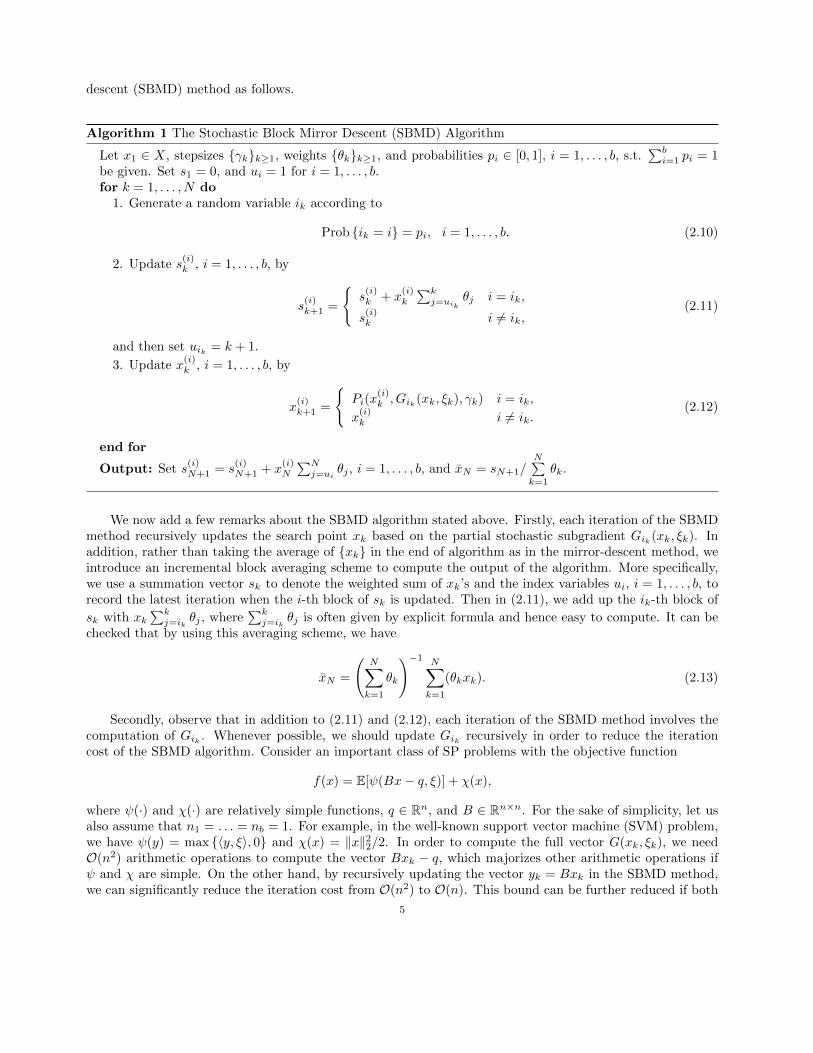
descent (SBMD) method as follows.

Algorithm 1 The Stochastic Block Mirror Descent (SBMD) Algorithm

Let x1 ∈ X, stepsizes {γk}k≥1, weights {θk}k≥1, and probabilities pi ∈ [0, 1], i = 1, . . . , b, s.t.∑bi=1 pi = 1

be given. Set s1 = 0, and ui = 1 for i = 1, . . . , b.for k = 1, . . . , N do

1. Generate a random variable ik according to

Prob {ik = i} = pi, i = 1, . . . , b. (2.10)

2. Update s(i)k , i = 1, . . . , b, by

s(i)k+1 =

{s

(i)k + x

(i)k

∑kj=uik

θj i = ik,

s(i)k i 6= ik,

(2.11)

and then set uik = k + 1.

3. Update x(i)k , i = 1, . . . , b, by

x(i)k+1 =

{Pi(x

(i)k , Gik(xk, ξk), γk) i = ik,

x(i)k i 6= ik.

(2.12)

end for

Output: Set s(i)N+1 = s

(i)N+1 + x

(i)N

∑Nj=ui

θj , i = 1, . . . , b, and xN = sN+1/N∑k=1

θk.

We now add a few remarks about the SBMD algorithm stated above. Firstly, each iteration of the SBMDmethod recursively updates the search point xk based on the partial stochastic subgradient Gik(xk, ξk). Inaddition, rather than taking the average of {xk} in the end of algorithm as in the mirror-descent method, weintroduce an incremental block averaging scheme to compute the output of the algorithm. More specifically,we use a summation vector sk to denote the weighted sum of xk’s and the index variables ui, i = 1, . . . , b, torecord the latest iteration when the i-th block of sk is updated. Then in (2.11), we add up the ik-th block of

sk with xk∑kj=ik

θj , where∑kj=ik

θj is often given by explicit formula and hence easy to compute. It can bechecked that by using this averaging scheme, we have

xN =

(N∑k=1

θk

)−1 N∑k=1

(θkxk). (2.13)

Secondly, observe that in addition to (2.11) and (2.12), each iteration of the SBMD method involves thecomputation of Gik . Whenever possible, we should update Gik recursively in order to reduce the iterationcost of the SBMD algorithm. Consider an important class of SP problems with the objective function

f(x) = E[ψ(Bx− q, ξ)] + χ(x),

where ψ(·) and χ(·) are relatively simple functions, q ∈ Rn, and B ∈ Rn×n. For the sake of simplicity, let usalso assume that n1 = . . . = nb = 1. For example, in the well-known support vector machine (SVM) problem,we have ψ(y) = max {〈y, ξ〉, 0} and χ(x) = ‖x‖22/2. In order to compute the full vector G(xk, ξk), we needO(n2) arithmetic operations to compute the vector Bxk − q, which majorizes other arithmetic operations ifψ and χ are simple. On the other hand, by recursively updating the vector yk = Bxk in the SBMD method,we can significantly reduce the iteration cost from O(n2) to O(n). This bound can be further reduced if both

5

ξk and B are sparse (i.e., the vector ξk and each row vector of B contain just a few nonzeros). The aboveexample can be generalized to the case when B has r × b blocks denoted by Bi,j ∈ Rmi×nj , 1 ≤ i ≤ r and1 ≤ j ≤ b, and each block row Bi = (Bi,1, . . . , Bi,b), i = 1, . . . , r, is block-sparse (see [29] for some relateddiscussion).

Thirdly, observe that the above SBMD method is conceptual only because we have not yet specified theselection of the stepsizes {γk}, the weights {θk}, and the probabilities {pi}. We will specify these parametersafter establishing some basic convergence properties of this method.

2.2. Convergence properties of SBMD for nonsmooth problems. In this subsection, we discussthe main convergence properties of the SBMD method for solving general nonsmooth convex problems.

Theorem 2.1. Let xN be the output of the SBMD algorithm and suppose that

θk = γk, k = 1, . . . , N. (2.14)

Then we have, for any N ≥ 1 and x ∈ X,

E[f(xN )− f(x)] ≤

(N∑k=1

γk

)−1 [ b∑i=1

p−1i Vi(x

(i)1 , x(i)) +

1

2

N∑k=1

γ2k

b∑i=1

M2i

], (2.15)

where the expectation is taken with respect to (w.r.t.) {ik} and {ξk}.Proof. For simplicity, let us denote Vi(z, x) ≡ Vi(z

(i), x(i)), gik ≡ g(ik)(xk) (c.f. (1.3)) and V (z, x) =b∑i=1

p−1i Vi(z, x). Also let us denote ζk = (ik, ξk) and ζ[k] = (ζ1, . . . , ζk). By the optimality condition of (2.5)

(e.g., Lemma 1 of [24]) and the definition of x(i)k in (2.12), we have

Vik(xk+1, x) ≤ Vik(xk, x) + γk⟨Gik(xk, ξk), UTik(x− xk)

⟩+

1

2γ2k ‖Gik(xk, ξk)‖2ik,∗.

Using this observation, we have, for any k ≥ 1 and x ∈ X,

V (xk+1, x) =∑i 6=ik

p−1i Vi(xk, x) + p−1

ikVik(xk+1, x)

≤∑i 6=ik

p−1i Vi(xk, x) + p−1

ik

[Vik(xk, x) + γk

⟨Gik(xk, ξk), UTik(x− xk)

⟩+ 1

2γ2k ‖Gik(xk, ξk)‖2ik,∗

]= V (xk, x) + γkp

−1ik〈UikGik(xk, ξk), x− xk〉+ 1

2γ2kp−1ik‖Gik(xk, ξk)‖2ik,∗

= V (xk, x) + γk〈g(xk), x− xk〉+ γkδk + 12γ

2k δk,

(2.16)

where

δk := 〈p−1ikUikGik(xk, ξk)− g(xk), x− xk〉 and δk := p−1

ik‖Gik(xk, ξk)‖2ik,∗ . (2.17)

It then follows from (2.16) and the convexity of f(·) that, for any k ≥ 1 and x ∈ X,

γk[f(xk)− f(x)] ≤ γk〈g(xk), xk − x〉 ≤ V (xk, x)− V (xk+1, x) + γkδk +1

2γ2k δk.

By using the above inequalities, the convexity of f(·), and the fact that xN =∑Nk=1(γkxk)/

∑Nk=1 γk due to

(2.13) and (2.14), we conclude that for any N ≥ 1 and x ∈ X,

f(xN )− f(x) ≤(

N∑k=1

γk

)−1∑Nk=1 γk [f(xk)− f(x)]

≤(

N∑k=1

γk

)−1 [V (x1, x) +

N∑k=1

(γkδk + 1

2γ2k δk)].

(2.18)

6

Now, observe that by (1.3) and (2.10),

Eζk[p−1ik〈UikGik , x− xk〉|ζ[k−1]

]=

∑bi=1 Eξk

[〈UiGi(xk, ξk), x− xk〉|ζ[k−1]

]=

∑bi=1〈Uigi(xk), x− xk〉 = 〈g(xk), x− xk〉,

and hence that

E[δk|ζk−1] = 0. (2.19)

Also, by (2.10) and (2.1),

E[p−1ik‖Gik(xk, ξk)‖2ik,∗

]=

b∑i=1

pip−1i ‖Gi(xk, ξk)‖2i,∗ ≤

b∑i=1

M2i . (2.20)

Our result in (2.15) then immediately follows by taking expectation on both sides of (2.18), and using theprevious observations in (2.19) and (2.20).

Below we provide a few specialized convergence results for the SBMD algorithm after properly selecting{pi}, {γk}, and {θk}.

Corollary 2.2. Suppose that {θk} in Algorithm 1 are set to (2.14).a) If X is bounded, and {pi} and {γk} are set to

pi =

√Di

b∑i=1

√Di, i = 1, . . . , b, and γk = γ ≡

√2

b∑i=1

√Di√

Nb∑i=1

M2i

, k = 1, . . . , N, (2.21)

then

E[f(xN )− f(x)] ≤√

2

N

b∑i=1

√Di

√√√√ b∑i=1

M2i ∀x ∈ X. (2.22)

b) If {pi} and {γk} are set to

pi =1

b, i = 1, . . . , b, and γk = γ ≡

√2bD√

Nb∑i=1

M2i

, k = 1, . . . , N, (2.23)

for some D > 0, then

E[f(xN )− f(x)] ≤

√√√√ b∑i=1

M2i

(∑bi=1 Vi(x

(i)1 , x

(i)∗ )

D+ D

) √b√

2N∀x ∈ X. (2.24)

Proof. We show part a) only, since part b) can be proved similarly. Note that by (2.7) and (2.21), we have

b∑i=1

p−1i Vi(x

(i)1 , x(i)) ≤

b∑i=1

p−1i Di ≤

(b∑i=1

√Di

)2

.

Using this observation, (2.15), and (2.21), we have

E[f(xN )− f(x∗)] ≤ (Nγ)−1

( b∑i=1

√Di

)2

+Nγ2

2

b∑i=1

M2i

=

√2

N

b∑i=1

√Di

√√√√ b∑i=1

M2i .

7

A few remarks about the results obtained in Theorem 2.1 and Corollary 2.2 are in place. First, theparameter setting in (2.21) only works for the case when X is bounded, while the one in (2.23) also applies tothe case when X is unbounded or when the bounds Di, i = 1, . . . , b, are not available. It can be easily seen

that the optimal choice of D in (2.24) would be

√∑bi=1 Vi(x

(i)1 , x

(i)∗ ). In this case, (2.24) reduces to

E[f(xN )− f(x)] ≤

√√√√2

b∑i=1

M2i

√√√√ b∑i=1

Vi(x(i)1 , x

(i)∗ )

√b√N≤

√√√√2

b∑i=1

M2i

√√√√ b∑i=1

Di√b√N, (2.25)

where the second inequality follows from (2.7). It is interesting to note the difference between the abovebound and (2.22). Specifically, the bound obtained in (2.22) by using a non-uniform distribution {pi} alwaysminorizes the one in (2.25) by the Cauchy-Schwartz inequality.

Second, observe that in view of (2.22), the total number of iterations required by the SBMD method tofind an ε-solution of (1.1) can be bounded by

2

(b∑i=1

√Di

)2( b∑i=1

M2i

)1

ε2. (2.26)

Also note that the iteration complexity of the mirror-descent SA algorithm employed with the same ωi(·),i = 1, . . . , b, is given by

2

b∑i=1

Di

(b∑i=1

M2i

)1

ε2. (2.27)

Clearly, the bound in (2.26) can be larger, up to a factor of b, than the one in (2.27). Therefore, the totalarithmetic cost of the SBMD algorithm will be comparable to or smaller than that of the mirror descent SA,if its iteration cost is smaller than that of the latter algorithm by a factor of O(b).

Third, in Corollary 2.2 we have used a constant stepsize policy where γ1 = . . . = γN . However, it shouldbe noted that variable stepsize policies, e.g., those similar to [24], can also be used in the SBMD method.

2.3. Convergence properties of SBMD for nonsmooth strongly convex problems. In this sub-section, we assume that the objective function f(·) in (1.1) is strongly convex, i.e., ∃ µ > 0 s.t.

f(y) ≥ f(x) + 〈g(x), y − x〉+µ

2‖y − x‖2 ∀x, y ∈ X. (2.28)

In order to establish the convergence of the SBMD algorithm for solving strongly convex problems, we needto assume that the prox-functions Vi(·, ·), i = 1, . . . , b, satisfy a quadratic growth condition (e.g., [12, 7, 8]):

Vi(z(i), x(i)) ≤ Q

2‖z(i) − x(i)‖2i ∀z(i), x(i) ∈ Xi, (2.29)

for some Q > 0. In addition, we need to assume that the probability distribution of ik is uniform, i.e.,

p1 = p2 = . . . = pb =1

b. (2.30)

Before proving the convergence of the SBMD algorithm for solving strongly convex problems, we firststate a simple technical result obtained by slightly modifying Lemma 3 of [15].

Lemma 2.3. Let ak ∈ (0, 1], k = 1, 2, . . ., be given. Also let us denote

Ak :=

{1 k = 1(1− ak)Ak−1 k ≥ 2.

(2.31)

8

Suppose that Ak > 0 for all k ≥ 2 and that the sequence {∆k} satisfies

∆k+1 ≤ (1− ak)∆k +Bk, k = 1, 2, . . . . (2.32)

Then, we have ∆k+1/Ak ≤ (1− a1)∆1 +∑ki=1(Bi/Ai).

We are now ready to describe the main convergence properties of the SBMD algorithm for solving nons-mooth strongly convex problems.

Theorem 2.4. Suppose that (2.28), (2.29), and (2.30) hold. If

γk ≤bQ

µ(2.33)

and

θk =γkΓk

with Γk =

{1 k = 1

Γk−1(1− γkµbQ ) k ≥ 2,

(2.34)

then, for any N ≥ 1 and x ∈ X, we have

E[f(xN )− f(x)] ≤

(N∑k=1

θk

)−1 [(b− γ1µ

Q)

b∑i=1

Vi(x(i)1 , x(i)) +

1

2

N∑k=1

γkθk

b∑i=1

M2i

]. (2.35)

Proof. For simplicity, let us denote Vi(z, x) ≡ Vi(z(i), x(i)), gik ≡ g(ik)(xk), and V (z, x) =

b∑i=1

p−1i Vi(z, x).

Also let us denote ζk = (ik, ξk) and ζ[k] = (ζ1, . . . , ζk), and let δk and δk be defined in (2.17). By (2.29) and(2.30), we have

V (z, x) = b

b∑i=1

Vi(z(i), x(i)) ≤ bQ

2

b∑i=1

‖z(i) − x(i)‖2i =bQ

2‖z − x‖2. (2.36)

Using this observation, (2.16), and (2.28), we obtain

V (xk+1, x) ≤ V (xk, x) + γk〈g(xk), x− xk〉+ γkδk +1

2γ2k δk

≤ V (xk, x) + γk

[f(x)− f(xk)− µ

2‖x− xk‖2

]+ γkδk +

1

2γ2k δk

≤(

1− γkµ

bQ

)V (xk, x) + γk [f(x)− f(xk)] + γkδk +

1

2γ2k δk,

which, in view of Lemma 2.3 (with ak = 1− γkµ/(bQ) and Ak = Γk), then implies that

1

ΓNV (xN+1, x) ≤

(1− γ1µ

bQ

)V (x1, x) +

N∑k=1

Γ−1k γk

[f(x)− f(xk) + δk +

1

2γ2k δk

]. (2.37)

Using the fact that V (xN+1, x) ≥ 0 and (2.34), we conclude from the above relation that

N∑k=1

θk[f(xk)− f(x)] ≤(

1− γ1µ

bQ

)V (x1, x) +

N∑k=1

θkδk +1

2

N∑k=1

γkθk δk. (2.38)

Taking expectation on both sides of the above inequality, and using relations (2.19) and (2.20), we obtain

N∑k=1

θkE[f(xk)− f(x)] ≤(

1− γ1µ

bQ

)V (x1, x) +

1

2

N∑k=1

γkθk

b∑i=1

M2i ,

9

which, in view of (2.13), (2.30) and the convexity of f(·), then clearly implies (2.35).

Below we provide a specialized convergence result for the SBMD method to solve nonsmooth stronglyconvex problems after properly selecting {γk}.

Corollary 2.5. Suppose that (2.28), (2.29) and (2.30) hold. If {θk} are set to (2.34) and {γk} are setto

γk =2bQ

µ(k + 1), k = 1, . . . , N, (2.39)

then, for any N ≥ 1 and x ∈ X, we have

E[f(xN )− f(x)] ≤ 2bQ

µ(N + 1)

b∑i=1

M2i . (2.40)

Proof. It can be easily seen from (2.34) and (2.39) that

Γk =2

k(k + 1), θk =

γkΓk

=bkQ

µ, b− γ1µ

Q= 0, (2.41)

N∑k=1

θk =bQN(N + 1)

2µ,

N∑k=1

γkθk ≤2b2Q2N

µ2, (2.42)

and

N∑k=1

θ2k =

b2Q2

µ2

N(N + 1)(2N + 1)

6≤ b2Q2

µ2

N(N + 1)2

3. (2.43)

Hence, by (2.35),

E[f(xN )− f(x)] ≤ 1

2

(N∑k=1

θk

)−1 N∑k=1

γkθk

b∑i=1

M2i ≤

2bQ

µ(N + 1)

b∑i=1

M2i .

In view of (2.40), the number of iterations performed by the SBMD method to find an ε-solution fornonsmooth strongly convex problems can be bound by

2b

µε

b∑i=1

M2i ,

which is comparable to the optimal bound obtained in [12, 7, 23] (up to a constant factor b). To the best ofour knowledge, no such complexity results have been obtained before for BCD type methods in the literature.

2.4. Large-deviation properties of SBMD for nonsmooth problems. Our goal in this subsectionis to establish the large-deviation results associated with the SBMD algorithm under the following “light-tail”assumption about the random variable ξ:

E{

exp[‖Gi(x, ξ)‖2i,∗ /M

2i

]}≤ exp(1), i = 1, 2, ..., b. (2.44)

It can be easily seen that (2.44) implies (2.1) by Jensen’s inequality. It should be pointed out that the above“light-tail” assumption is alway satisified for determinisitc problems with bounded subgradients.

For the sake of simplicity, we only consider the case when the random variables {ik} in the SBMD agorithmare uniformly distributed, i.e., relation (2.30) holds. The following result states the large-deviation propertiesof the SBMD algorithm for solving general nonsmooth problems without assuming strong convexity.

Theorem 2.6. Suppose that Assumptions (2.44) and (2.30) holds. Also assume that X is bounded.

10

a) For solving general nonsmooth CP problems (i.e., (2.14) holds), we have

Prob

{f(xN )− f(x) ≥ b

(N∑k=1

γk

)−1 [ b∑i=1

Vi(x(i)1 , x(i)) + M2

N∑k=1

γ2k

+λM2

(N∑k=1

γ2k + 32 b

b∑i=1

Di

√N∑k=1

γ2k

)]}≤ exp

(−λ2/3

)+ exp(−λ),

(2.45)

for any N ≥ 1, x ∈ X and λ > 0, where M = maxi=1,...,b

Mi.

b) For solving strongly convex problems (i.e., (2.28), (2.29), (2.33), and (2.34) hold), we have

Prob

{f(xN )− f(x) ≥ b

(N∑k=1

θk

)−1 [(b− γ1µ

Q )b∑i=1

Vi(x(i)1 , x(i)) + M2

N∑k=1

γkθk

+λM2

(N∑k=1

γkθk + 32bb∑i=1

Di

√N∑k=1

θ2k

)]}≤ exp

(−λ2/3

)+ exp(−λ),

(2.46)

for any N ≥ 1, x ∈ X and λ > 0.

Proof. We first show part a). Note that by (2.44), the concavity of φ(t) =√t for t ≥ 0 and the Jensen’s

inequality, we have, for any i = 1, 2, ..., b,

E{

exp[‖Gi(x, ξ)‖2i,∗ /(2M

2i )]}≤√E{

exp[‖Gi(x, ξ)‖2i,∗ /M2

i

]}≤ exp(1/2). (2.47)

Also note that by (2.19), δk, k = 1, . . . , N , is the martingale-difference. In addition, denoting M2 ≡32 b2M2

∑bi=1Di, we have

E[exp(M−2δ2

k

)] ≤

b∑i=1

piE[exp

(M−2‖x− xk‖2 ‖p−1

i UTi Gi − g(xk)‖2∗)]

(by (2.10), (2.17))

≤b∑i=1

piE{

exp[2M−2‖x− xk‖2

(b2‖Gi‖2∗ + ‖g(xk)‖2∗

)]}(by definition of Ui and (2.30))

≤b∑i=1

piE

{exp

[16M−2

(b∑i=1

Di

)(b2‖Gi‖2∗ +

b∑i=1

M2i

)]}(by (2.3) and (2.9))

≤b∑i=1

piE

{exp

[b2‖Gi‖2∗ +

∑bi=1M

2i

2b2M2

]}(by definition of M)

≤b∑i=1

piE{

exp

[‖Gi‖2∗2M2

i

+1

2

]}≤ exp(1). (by (2.47))

Therefore, by the well-known large-deviation theorem on the Martingale-difference (see, e.g., Lemma 2 of [18]),we have

Prob

N∑k=1

γkδk ≥ λM

√√√√ N∑k=1

γ2k

≤ exp(−λ2/3). (2.48)

11

Also observe that under Assumption (2.44),

E[exp

(δk/(bM

2))]≤

b∑i=1

piE[exp

(‖Gi(xk, ξk)‖2i,∗ /M

2)]

(by (2.10), (2.17), (2.30))

≤b∑i=1

piE[exp

(‖Gi(xk, ξk)‖2i,∗ /M

2i

)](by definition of M)

≤b∑i=1

pi exp(1) = exp(1). (by (2.1))

Setting πk = γ2k/∑Nk=1 γ

2k, we have exp

{∑Nk=1 πk δk/(bM

2)}≤∑Nk=1 πk exp{δk/(bM2)}. Using these previous

two inequalities, we have

E

[exp

{N∑k=1

γ2k δk/(bM

2N∑k=1

γ2k)

}]≤ exp{1}.

It then follows from Markov’s inequality that

∀λ ≥ 0 : Prob

{N∑k=1

γ2k δk > (1 + λ)(bM2)

N∑k=1

γ2k

}≤ exp{−λ}. (2.49)

Combining (2.18), (2.48) and (2.49), we obtain (2.45).The probabilistic bound in (2.46) follows from (2.38) and an argument similar to the one used in the proof

of (2.45), and hence the details are skipped.

We now provide some specialized large-deviation results for the SBMD algorithm with different selectionsof {γk} and {θk}.

Corollary 2.7. Suppose that (2.44) and (2.30) hold. Also assume that X is bounded.a) If {θk} and {γk} are set to (2.14) and (2.23) for general nonsmooth problems, then we have

Prob

{f(xN )− f(x) ≥ b

√∑bi=1M

2i√

2NbD2

(2bD2 +

∑bi=1Di + 2λbD2

)+

32λb52 M2 ∑b

i=1Di√NbD2

}≤ exp

(−λ2/3

)+ exp(−λ)

(2.50)

for any x ∈ X and λ > 0.b) If {θk} and {γk} are set to (2.34) and (2.39) for strongly convex problems, then we have

Prob{f(xN )− f(x) ≥ 4(1+λ)b2M2Q

(N+1)µ +64λb2M2 ∑b

i=1Di√3N

}≤ exp

(−λ2/3

)+ exp(−λ) (2.51)

for any x ∈ X and λ > 0.

Proof. Note that by (2.7), we haveb∑i=1

Vi(x(i)1 , x(i)) ≤

∑bi=1Di. Also by (2.23), we have

N∑k=1

γk =

(2NbD2∑bi=1M

2i

) 12

and

N∑k=1

γ2k =

2bD2∑bi=1M

2i

.

Using these identities and (2.45), we conclude that

Prob

{f(xN )− f(x) ≥ b

(∑bi=1M

2i

2NbD2

) 12

[b∑i=1

Di + 2bD2M2

(b∑i=1

M2i

)−1

+λM2

(2bD2

(b∑i=1

M2i

)−1

+ 32√

2 b32 D

b∑i=1

Di(

b∑i=1

M2i

)− 12

)]}≤ exp

(−λ2/3

)+ exp(−λ).

12

Using the fact that M2 ≤∑bi=1M

2i and simplifying the above relation, we obtain (2.50). Similarly, relation

(2.51) follows directly from (2.46) and a few bounds in (2.41), (2.42) and (2.43).

We now add a few remarks about the results obtained in Theorem 2.6 and Corollary 2.7. Firstly, observethat by (2.48), the number of iterations required by the SBMD method to find an (ε, λ)-solution of (1.1), i.e.,a point x ∈ X s.t. Prob{f(x)− f∗ ≥ ε} ≤ λ can be bounded by

O(

log2(1/λ)

ε2

)

after disregarding a few constant factors. To the best of our knowledge, now such large-deviation results havebeen obtained before for the BCD methods for solving general nonsmooth CP problems, although similarresults have been established for solving smooth problems or some composite problems [28, 33].

Secondly, it follows from (2.46) that the number of iterations performed by the SBMD method to findan (ε, λ)-solution for nonsmooth strongly convex problems, after disregarding a few constant factors, can bebounded by O

(log2(1/λ)/ε2

), which is about the same as the one obtained for solving nonsmooth problems

without assuming convexity. It should be noted, however, that this bound can be improved to O (log(1/λ)/ε) ,for example, by incorporating a domain shrinking procedure [8].

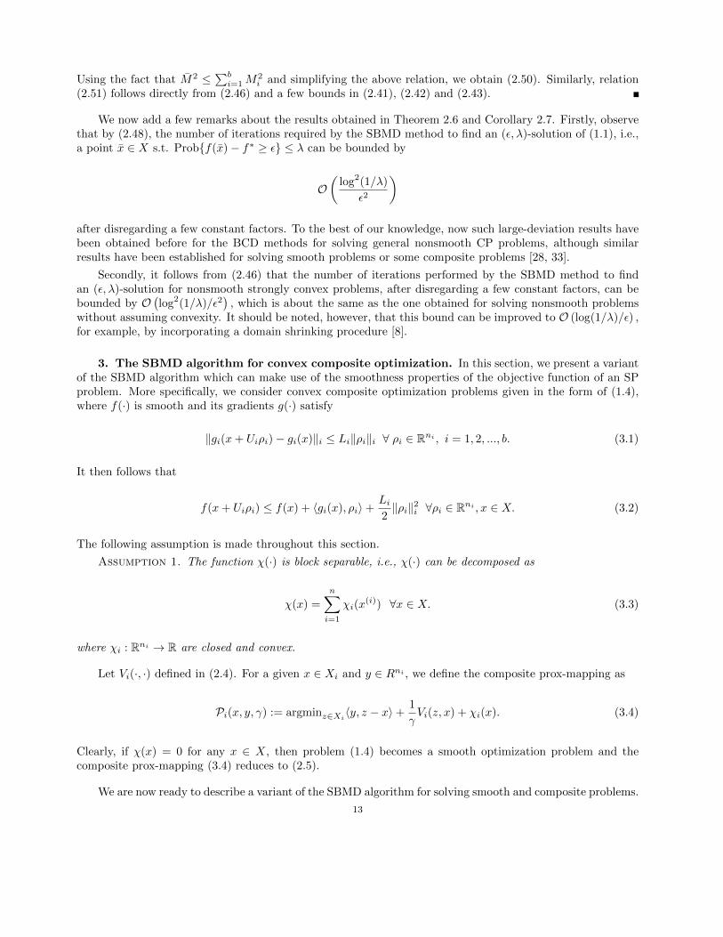
3. The SBMD algorithm for convex composite optimization. In this section, we present a variantof the SBMD algorithm which can make use of the smoothness properties of the objective function of an SPproblem. More specifically, we consider convex composite optimization problems given in the form of (1.4),where f(·) is smooth and its gradients g(·) satisfy

‖gi(x+ Uiρi)− gi(x)‖i ≤ Li‖ρi‖i ∀ ρi ∈ Rni , i = 1, 2, ..., b. (3.1)

It then follows that

f(x+ Uiρi) ≤ f(x) + 〈gi(x), ρi〉+Li2‖ρi‖2i ∀ρi ∈ Rni , x ∈ X. (3.2)

The following assumption is made throughout this section.

Assumption 1. The function χ(·) is block separable, i.e., χ(·) can be decomposed as

χ(x) =

n∑i=1

χi(x(i)) ∀x ∈ X. (3.3)

where χi : Rni → R are closed and convex.

Let Vi(·, ·) defined in (2.4). For a given x ∈ Xi and y ∈ Rni , we define the composite prox-mapping as

Pi(x, y, γ) := argminz∈Xi〈y, z − x〉+

1

γVi(z, x) + χi(x). (3.4)

Clearly, if χ(x) = 0 for any x ∈ X, then problem (1.4) becomes a smooth optimization problem and thecomposite prox-mapping (3.4) reduces to (2.5).

We are now ready to describe a variant of the SBMD algorithm for solving smooth and composite problems.

13

Algorithm 2 A variant of SBMD for convex stochastic composite optimization

Let x1 ∈ X, stepsizes {γk}k≥1, weights {θk}k≥1, and probabilities pi ∈ [0, 1], i = 1, . . . , b, s.t.∑bi=1 pi = 1

be given. Set s1 = 0, ui = 1 for i = 1, . . . , b, and θ1 = 0.for k = 1, . . . , N do

1. Generate a random variable ik according to (2.10).

2. Update s(i)k , i = 1, . . . , b, by (2.11) and then set uik = k + 1.

3. Update x(i)k , i = 1, . . . , b, by

x(i)k+1 =

{Pik(x

(i)k , Gik(xk, ξk), γk) i = ik,

x(i)k i 6= ik.

(3.5)

end for

Output: Set s(i)N+1 = s

(i)N+1 + x

(i)N+1

∑N+1j=ui

θj , i = 1, . . . , b, and xN = sN+1/N+1∑k=1

θk.

A few remarks about the above variant of SBMD algorithm for composite convex problem in place. Firstly,similar to Algorithm 1, G(xk, ξk) is an unbiased estimator of g(xk) (i.e., (1.3) holds). Moreover, in order toknow exactly the effect of stochastic noises in G(xk, ξk), we assume that for some σi ≥ 0,

E[‖Gi(x, ξ)− gi(x)‖2i,∗] ≤ σ2i , i = 1, . . . , b. (3.6)

Clearly, if σi = 0, i = 1, . . . , b, then the problem is deterministic. For notational convenience, we also denote

σ :=( b∑i=1

σ2i

) 12

. (3.7)

Secondly, observe that the way we compute the output xN in Algorithm 2 is slightly different fromAlgorithm 1. In particular, we set θ1 = 0 and compute xN of Algorithm 2 as a weighted average of the searchpoints x2, ..., xN+1, i.e.,

xN =

(N+1∑k=2

θk

)−1

sN+1 =

(N+1∑k=2

θk

)−1 N+1∑k=2

(θkxk), (3.8)

while the output of Algorithm 1 is taken as a weighted average of x1, ..., xN .

Thirdly, it can be easily seen from (2.7), (3.1), and (3.6) that if X is bounded, then

E[‖Gi(x, ξ)‖2i,∗] ≤ 2‖gi(x)‖2i,∗ + 2E‖Gi(x, ξ)− gi(x)‖2i,∗] ≤ 2‖gi(x)‖2i,∗ + 2σ2i

≤ 2[2‖gi(x)− gi(x1)‖2i,∗ + 2‖gi(x1)‖2i,∗

]+ 2σ2

i

≤ 4L2i ‖x− x1‖2i,∗ + 4‖gi(x1)‖2i,∗ + 2σ2

i

≤ 8L2iDi + 4‖gi(x1)‖2i,∗ + 2σ2

i , i = 1, . . . , b. (3.9)

Hence, we can directly apply Algorithm 1 in the previous section to problem (1.4), and its rate of convergenceis readily given by Theorem 2.1 and 2.4. However, in this section we will show that by properly selecting {θk},{γk}, and {pi} in the above variant of the SBMD algorithm, we can significantly improve the dependence ofthe rate of convergence of the SBMD algorithm on the Lipschitz constants Li, i = 1, . . . , b.

We first discuss the main convergence properties of Algorithm 2 for convex stochastic composite optimiza-tion without assuming strong convexity.

14

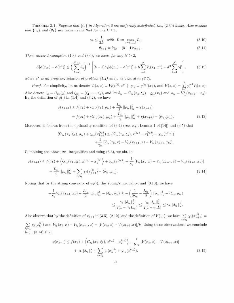
Theorem 3.1. Suppose that {ik} in Algorithm 2 are uniformly distributed, i.e., (2.30) holds. Also assumethat {γk} and {θk} are chosen such that for any k ≥ 1,

γk ≤1

2Lwith L := max

i=1,...,bLi, (3.10)

θk+1 = bγk − (b− 1)γk+1. (3.11)

Then, under Assumption (1.3) and (3.6), we have, for any N ≥ 2,

E[φ(xN )− φ(x∗)] ≤(N+1∑k=2

θk

)−1[

(b− 1)γ1[φ(x1)− φ(x∗)] + b

b∑i=1

Vi(x1, x∗) + σ2

N∑k=1

γ2k

], (3.12)

where x∗ is an arbitrary solution of problem (1.4) and σ is defined in (3.7).

Proof. For simplicity, let us denote Vi(z, x) ≡ Vi(z(i), x(i)), gik ≡ g(ik)(xk), and V (z, x) =

b∑i=1

p−1i Vi(z, x).

Also denote ζk = (ik, ξk) and ζ[k] = (ζ1, . . . , ζk), and let δik = Gik(xk, ξk)− gik(xk) and ρik = UTik(xk+1 − xk).By the definition of φ(·) in (1.4) and (3.2), we have

φ(xk+1) ≤ f(xk) + 〈gik(xk), ρik〉+Lik2‖ρik‖

2ik

+ χ(xk+1)

= f(xk) + 〈Gik(xk), ρik〉+Lik2‖ρik‖

2ik

+ χ(xk+1)− 〈δik , ρik〉. (3.13)

Moreover, it follows from the optimality condition of (3.4) (see, e.g., Lemma 1 of [14]) and (3.5) that

〈Gik(xk, ξk), ρik〉+ χik(x(ik)k+1) ≤ 〈Gik(xk, ξk), x(ik) − x(ik)

k 〉+ χik(x(ik))

+1

γk[Vik(xk, x)− Vik(xk+1, x)− Vik(xk+1, xk)] .

Combining the above two inequalities and using (3.3), we obtain

φ(xk+1) ≤ f(xk) +⟨Gik(xk, ξk), x(ik) − x(ik)

k

⟩+ χik(x(ik)) +

1

γk[Vik(xk, x)− Vik(xk+1, x)− Vik(xk+1, xk)]

+Lik2‖ρik‖

2ik

+∑i 6=ik

χi(x(i)k+1)− 〈δik , ρik〉. (3.14)

Noting that by the strong convexity of ωi(·), the Young’s inequality, and (3.10), we have

− 1

γkVik(xk+1, xk) +

Lik2‖ρik‖

2ik− 〈δik , ρik〉 ≤ −

(1

2γk− Lik

2

)‖ρik‖

2ik− 〈δik , ρik〉

≤γk ‖δik‖

2∗

2(1− γkLik)≤

γk ‖δik‖2∗

2(1− γkL)≤ γk ‖δik‖

2∗ .

Also observe that by the definition of xk+1 in (3.5), (2.12), and the definition of V (·, ·), we have∑i 6=ik

χi(x(i)k+1) =∑

i6=ikχi(x

(i)k ) and Vik(xk, x)− Vik(xk+1, x) = [V (xk, x)− V (xk+1, x)]/b. Using these observations, we conclude

from (3.14) that

φ(xk+1) ≤ f(xk) +⟨Gik(xk, ξk), x(ik) − x(ik)

k

⟩+

1

bγk[V (xk, x)− V (xk+1, x)]

+ γk ‖δik‖2∗ +

∑i 6=ik

χi(x(i)k ) + χik(x(ik)). (3.15)

15

Now noting that

Eζk[⟨Gik(xk, ξk), x(ik) − x(ik)

k

⟩|ζ[k−1]

]=

1

b

b∑i=1

Eξk[⟨Gi(xk, ξk), x(i) − x(i)

k

⟩|ζ[k−1]

]=

1

b〈g(xk), x− xk〉 ≤

1

b[f(x)− f(xk)], (3.16)

Eζk[‖δik‖

2∗ |ζ[k−1]

]=

1

b

b∑i=1

Eξk[‖Gi(xk, ξk)− gi(xk)‖2i,∗|ζ[k−1]

]≤ 1

b

b∑i=1

σ2i =

σ2

b, (3.17)

Eζk

∑i 6=ik

χi(x(i)k )|ζ[k−1]

=1

b

b∑j=1

∑i 6=j

χi(x(i)k ) =

b− 1

bχ(xk), (3.18)

Eζk[χik(x(ik))|ζ[k−1]

]=

1

b

b∑i=1

χi(x(i) =

1

bχ(x), (3.19)

we conclude from (3.15) that

Eζk[φ(xk+1) +

1

bγkV (xk+1, x)|ζ[k−1]

]≤ f(xk) +

1

b[f(x)− f(xk)] +

1

bχ(x) +

1

bγk[V (xk, x)]

+γkbσ2 +

b− 1

bχ(xk) +

1

bχ(x)

=b− 1

bφ(xk) +

1

bφ(x) +

1

bγk[V (xk, x)− V (xk+1, x)] +

γkbσ2,

which implies that

bγkE[φ(xk+1)− φ(x)] + E[V (xk+1, x)] ≤ (b− 1)γkE[φ(xk)− φ(x)] + E [V (xk, x)] + γ2kσ

2. (3.20)

Now, summing up the above inequalities (with x = x∗) for k = 1, . . . , N , and noting that θk+1 = bγk − (b−1)γk+1, we obtain

N∑k=2

θkE[φ(xk)−φ(x∗)]+bγNE[φ(xN+1)−φ(x∗)]+E[V (xN+1, x)] ≤ (b−1)γ1[φ(x1)−φ(x∗)]+V (x1, x∗)+σ2

N∑k=1

γ2k,

Using the above inequality and the facts that V (·, ·) ≥ 0 and φ(xN+1) ≥ φ(x∗), we conclude

N+1∑k=2

θkE[φ(xk)− φ(x∗)] ≤ (b− 1)γ1[φ(x1)− φ(x∗)] + V (x1, x∗) + σ2

N∑k=1

γ2k,

which, in view of (3.7), (3.8) and the convexity of φ(·), clearly implies (3.12).

The following corollary describes a specialized convergence result of Algorithm 2 for solving convex stochas-tic composite optimization problems after properly selecting {γk}.

Corollary 3.2. Suppose that {pi} in Algorithm 2 are set to (2.30). Also assume that {γk} are set to

γk = γ = min

{1

2L,D

σ

√b

N

}(3.21)

for some D > 0, and {θk} are set to (3.11). Then, under Assumptions (1.3) and (3.6), we have

E [φ(xN )− φ(x∗)] ≤ (b− 1)[φ(x1)− φ(x∗)]

N+

2bL∑bi=1 Vi(x1, x

∗)

N

+σ√b√N

[∑bi=1 Vi(x1, x

∗)

D+ D

]. (3.22)

16

where x∗ is the optimal solution of problem (1.4).Proof. It follows from (3.11) and (3.21) that θk = γk = γ, k = 1, . . . , N . Using this observation and

Theorem 3.1, we obtain

E [φ(xN )− φ(x∗)] ≤ (b− 1)[φ(x1)− φ(x∗)]

N+b∑bi=1 Vi(x1, x

∗)

Nγ+ γσ2,

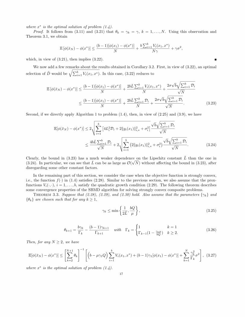
which, in view of (3.21), then implies (3.22).

We now add a few remarks about the results obtained in Corollary 3.2. First, in view of (3.22), an optimal

selection of D would be√∑b

i=1 Vi(x1, x∗). In this case, (3.22) reduces to

E [φ(xN )− φ(x∗)] ≤ (b− 1)[φ(x1)− φ(x∗)]

N+

2bL∑bi=1 Vi(x1, x

∗)

N+

2σ√b√∑b

i=1Di√N

≤ (b− 1)[φ(x1)− φ(x∗)]

N+

2bL∑bi=1DiN

+2σ√b√∑b

i=1Di√N

. (3.23)

Second, if we directly apply Algorithm 1 to problem (1.4), then, in view of (2.25) and (3.9), we have

E[φ(xN )− φ(x∗)] ≤ 2

√√√√ b∑i=1

[4L2

iDi + 2‖gi(x1)‖2i,∗ + σ2i

]√b√∑bi=1Di√N

≤4bL

∑bi=1Di√N

+ 2

√√√√ b∑i=1

(2‖gi(x1)‖2i,∗ + σ2

i

)√b√∑bi=1Di√N

. (3.24)

Clearly, the bound in (3.23) has a much weaker dependence on the Lipschitz constant L than the one in(3.24). In particular, we can see that L can be as large as O(

√N) without affecting the bound in (3.23), after

disregarding some other constant factors.

In the remaining part of this section, we consider the case when the objective function is strongly convex,i.e., the function f(·) in (1.4) satisfies (2.28). Similar to the previous section, we also assume that the prox-functions Vi(·, ·), i = 1, . . . , b, satisfy the quadratic growth condition (2.29). The following theorem describessome convergence properties of the SBMD algorithm for solving strongly convex composite problems.

Theorem 3.3. Suppose that (2.28), (2.29), and (2.30) hold. Also assume that the parameters {γk} and{θk} are chosen such that for any k ≥ 1,

γk ≤ min

{1

2L,bQ

µ

}, (3.25)

θk+1 =bγkΓk− (b− 1)γk+1

Γk+1with Γk =

{1 k = 1

Γk−1(1− γkµbQ ) k ≥ 2.

(3.26)

Then, for any N ≥ 2, we have

E[φ(xN )− φ(x∗)] ≤

[N+1∑k=2

θk

]−1 [(b− µγ1Q

) b∑i=1

Vi(x1, x∗) + (b− 1)γ1[φ(x1)− φ(x∗)] +

N∑k=1

γ2k

Γkσ2

], (3.27)

where x∗ is the optimal solution of problem (1.4).

17

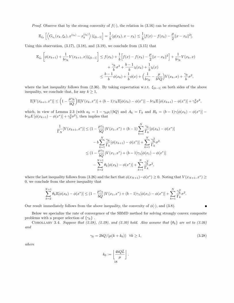
Proof. Observe that by the strong convexity of f(·), the relation in (3.16) can be strengthened to

Eζk[⟨Gik(xk, ξk), x(ik) − x(ik)

k

⟩|ζ[k−1]

]=

1

b〈g(xk), x− xk〉 ≤

1

b[f(x)− f(xk)− µ

2‖x− xk‖2].

Using this observation, (3.17), (3.18), and (3.19), we conclude from (3.15) that

Eζk[φ(xk+1) +

1

bγkV (xk+1, x)|ζ[k−1]

]≤ f(xk) +

1

b

[f(x)− f(xk)− µ

2‖x− xk‖2

]+

1

bγkV (xk, x)

+γkbσ2 +

b− 1

bχ(xk) +

1

bχ(x)

≤ b− 1

bφ(xk) +

1

bφ(x) +

( 1

bγk− µ

b2Q

)V (xk, x) +

γkbσ2,

where the last inequality follows from (2.36). By taking expectation w.r.t. ξ[k−1] on both sides of the aboveinequality, we conclude that, for any k ≥ 1,

E[V (xk+1, x∗)] ≤

(1− µγk

bQ

)E[V (xk, x

∗)] + (b− 1)γkE[φ(xk)− φ(x∗)]− bγkE [φ(xk+1)− φ(x∗)] + γ2kσ

2,

which, in view of Lemma 2.3 (with ak = 1 − γkµ/(bQ) and Ak = Γk and Bk = (b − 1)γ[φ(xk) − φ(x∗)] −bγkE [φ(xk+1)− φ(x∗)] + γ2

kσ2), then implies that

1

ΓN[V (xk+1, x

∗)] ≤ (1− µγ1

bQ)V (x1, x

∗) + (b− 1)

N∑k=1

γkΓk

[φ(xk)− φ(x∗)]

− bN∑k=1

γkΓk

[φ(xk+1)− φ(x∗)] +

N∑k=1

γ2k

Γkσ2

≤ (1− µγ1

bQ)V (x1, x

∗) + (b− 1)γ1[φ(x1)− φ(x∗)]

−N+1∑k=2

θk[φ(xk)− φ(x∗)] +

N∑k=1

γ2k

Γkσ2,

where the last inequality follows from (3.26) and the fact that φ(xN+1)−φ(x∗) ≥ 0. Noting that V (xN+1, x∗) ≥

0, we conclude from the above inequality that

N+1∑k=2

θkE[φ(xk)− φ(x∗)] ≤ (1− µγ1

bQ)V (x1, x

∗) + (b− 1)γ1[φ(x1)− φ(x∗)] +

N∑k=1

γ2k

Γkσ2.

Our result immediately follows from the above inequality, the convexity of φ(·), and (3.8).

Below we specialize the rate of convergence of the SBMD method for solving strongly convex compositeproblems with a proper selection of {γk} .

Corollary 3.4. Suppose that (2.28), (2.29), and (2.30) hold. Also assume that {θk} are set to (3.26)and

γk = 2bQ/(µ(k + k0)) ∀k ≥ 1, (3.28)

where

k0 :=

⌊4bQL

µ

⌋.

18

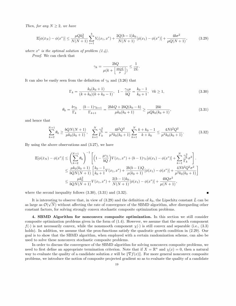
Then, for any N ≥ 2, we have

E[φ(xN )− φ(x∗)] ≤ µQk20

N(N + 1)

b∑i=1

Vi(x1, x∗) +

2Q(b− 1)k0

N(N + 1)[φ(x1)− φ(x∗)] +

4bσ2

µQ(N + 1), (3.29)

where x∗ is the optimal solution of problem (1.4).

Proof. We can check that

γk =2bQ

µ(k +⌊

4bQLµ

⌋)≤ 1

2L.

It can also be easily seen from the definition of γk and (3.26) that

Γk =k0(k0 + 1)

(k + k0)(k + k0 − 1), 1− γ1µ

bQ=k0 − 1

k0 + 1, ∀k ≥ 1, (3.30)

θk =bγkΓk− (b− 1)γk+1

Γk+1=

2bkQ+ 2bQ(k0 − b)µk0(k0 + 1)

≥ 2bk

µQk0(k0 + 1), (3.31)

and hence that

N+1∑k=2

θk ≥bQN(N + 1)

µk0(k0 + 1),

N∑k=1

γ2k

Γk=

4b2Q2

µ2k0(k0 + 1)

N∑k=1

k + k0 − 1

k + k0≤ 4Nb2Q2

µ2k0(k0 + 1). (3.32)

By using the above observations and (3.27), we have

E[φ(xN )− φ(x∗)] ≤

(N+1∑k=2

θk

)−1 [(1− µγ1

bQ

)V (x1, x

∗) + (b− 1)γ1[φ(x1)− φ(x∗)] +

N∑k=1

γ2k

Γkσ2

].

≤ µk0(k0 + 1)

bQN(N + 1)

[k0 − 1

k0 + 1V (x1, x

∗) +2b(b− 1)Q

µ(k0 + 1)[φ(x1)− φ(x∗)] +

4Nb2Q2σ2

µ2k0(k0 + 1)

]≤ µk2

0

bQN(N + 1)V (x1, x

∗) +2(b− 1)k0

N(N + 1)[φ(x1)− φ(x∗)] +

4bQσ2

µ(N + 1),

where the second inequality follows (3.30), (3.31) and (3.32).

It is interesting to observe that, in view of (3.29) and the definition of k0, the Lipschitz constant L can beas large as O(

√N) without affecting the rate of convergence of the SBMD algorithm, after disregarding other

constant factors, for solving strongly convex stochastic composite optimization problems.

4. SBMD Algorithm for nonconvex composite optimization. In this section we still considercomposite optimization problems given in the form of (1.4). However, we assume that the smooth componentf(·) is not necessarily convex, while the nonsmooth component χ(·) is still convex and separable (i.e., (3.3)holds). In addition, we assume that the prox-functions satisfy the quadratic growth condition in (2.29). Ourgoal is to show that the SBMD algorithm, when employed with a certain randomization scheme, can also beused to solve these nonconvex stochastic composite problems.

In order to discuss the convergence of the SBMD algorithm for solving nonconvex composite problems, weneed to first define an appropriate termination criterion. Note that if X = Rn and χ(x) = 0, then a naturalway to evaluate the quality of a candidate solution x will be ‖∇f(x)‖. For more general nonconvex compositeproblems, we introduce the notion of composite projected gradient so as to evaluate the quality of a candidate

19

solution (see [26, 16, 17, 6, 10] for some related discussions). More specifically, for a given x ∈ X, y ∈ Rn anda constant γ > 0, we define G(x, y, γ) ≡ (G1(x, y, γ), . . . ,Gb(x, y, γ)) by

Gi(x, y, γ) :=1

γ[UTi x− Pi(UTi x, UTi y, γ)], i = 1, . . . , b, (4.1)

where Pi is defined in (3.4). In particular, if y = g(x), then we call G(x, g(x), γ) the composite projectedgradient of x w.r.t. γ. It can be easily seen that G(x, g(x), γ) = g(x) when X = Rn and χ(x) = 0. Proposi-tion 4.1 below relates the composite projected gradient to the first-order optimality condition of the compositeproblem under a more general setting.

Proposition 4.1. Let x ∈ X be given and G(x, y, γ) be defined as in (4.1) for some γ > 0. Also let usdenote x+ := x− γG(x, g(x), γ). Then there exists pi ∈ ∂χi(UTi x+) s.t.

UTi g(x+) + pi ∈ −NXi(UTi x

+) + Bi ((Li +Qγ)‖G(x, g(x), γ)‖i) , i = 1, . . . , b, (4.2)

where Bi(ε) := {v ∈ Rni : ‖v‖i,∗ ≤ ε} and NXidenotes the normal cone of Xi at UTi x.

Proof. By the definition of x+, (3.4), and (4.1), we have UTi x+ = Pi(UTi x, UTi g(x), γ). Using the above

relation and the optimality condition of (3.4), we conclude that there exists pi ∈ ∂χi(UTi x+) s.t.

〈UTi g(x) +1

γ

[∇ωi(UTi x+)−∇ωi(UTi x)

]+ pi, u− UTi x+〉 ≥ 0, ∀u ∈ Xi.

Now, denoting ζ = UTi [g(x) − g(x+) + 1γ

[∇ωi(UTi x+)−∇ωi(UTi x+)

], we conclude from the above relation

that UTi g(x+) + pi + ζ ∈ −NXi(UTi x

+). Also noting that, by ‖UTi [g(x+)− g(x)]‖i,∗ ≤ Li‖UTi (x+ − x)‖i and‖∇ωi(UTi x+)−∇ωi(UTi x+)‖i,∗ ≤ Q‖UTi (x+ − x)‖i,

‖ζ‖i,∗ ≤(Li +

Q

γ

)‖UTi (x+ − x)‖i =

(Li +

Q

γ

)γ‖UTi G(x, g(x), γ)‖i

= (Li +Qγ)‖UTi G(x, g(x), γ)‖i.

Relation (4.2) then immediately follows from the above two relations.

A common practice in the gradient descent methods for solving nonconvex problems (for the simple casewhen X = Rn and χ(x) = 0) is to choose the output solution xN so that

‖g(xN )‖∗ = mink=1,...,N

‖g(xk)‖∗, (4.3)

where xk, k = 1, . . . , N , is the trajectory generated by the gradient descent method (see, e.g., [26]). However,such a procedure requires the computation of the whole vector g(xk) at each iteration and hence can beexpensive if n is large. In this section, we address this problem by introducing a randomization schemeinto the SBMD algorithm as follows. Instead of taking the best solution from the trajectory as in (4.3), werandomly select xN from x1, . . . , xN according to a certain probability distribution. The basic scheme of thisalgorithm is described as follows.

20

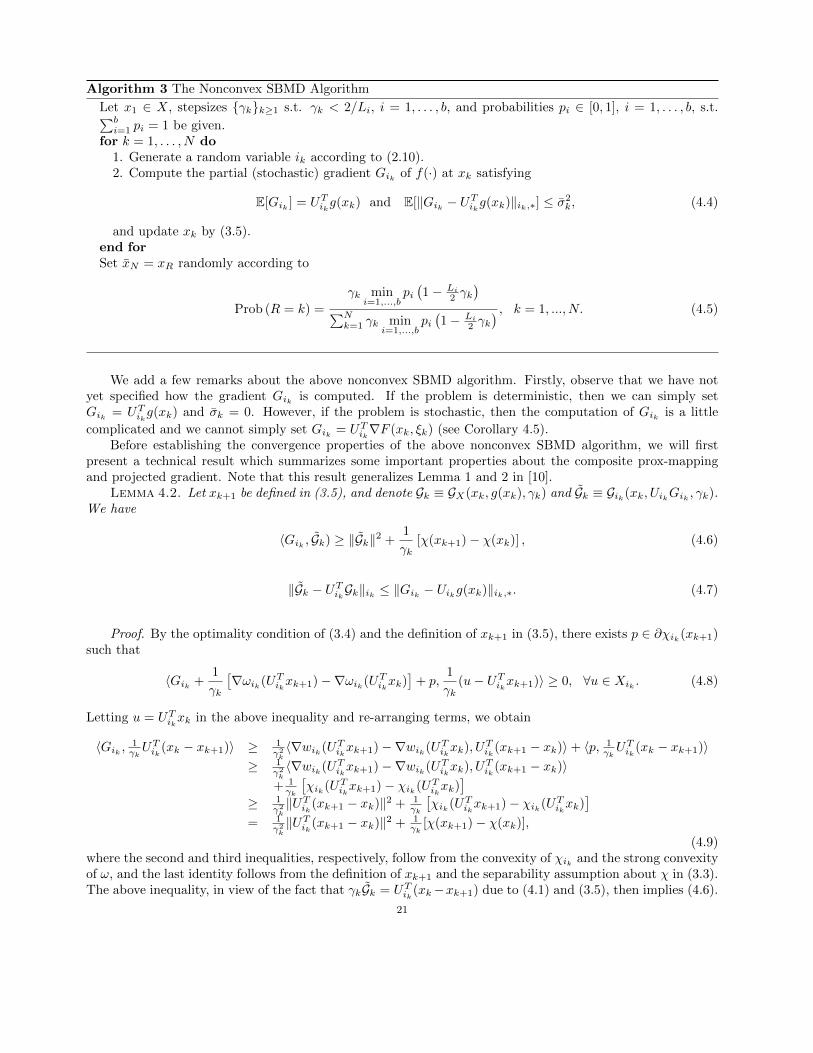
Algorithm 3 The Nonconvex SBMD Algorithm

Let x1 ∈ X, stepsizes {γk}k≥1 s.t. γk < 2/Li, i = 1, . . . , b, and probabilities pi ∈ [0, 1], i = 1, . . . , b, s.t.∑bi=1 pi = 1 be given.

for k = 1, . . . , N do1. Generate a random variable ik according to (2.10).2. Compute the partial (stochastic) gradient Gik of f(·) at xk satisfying

E[Gik ] = UTikg(xk) and E[‖Gik − UTikg(xk)‖ik,∗] ≤ σ2k, (4.4)

and update xk by (3.5).end forSet xN = xR randomly according to

Prob (R = k) =

γk mini=1,...,b

pi(1− Li

2 γk)

∑Nk=1 γk min

i=1,...,bpi(1− Li

2 γk) , k = 1, ..., N. (4.5)

We add a few remarks about the above nonconvex SBMD algorithm. Firstly, observe that we have notyet specified how the gradient Gik is computed. If the problem is deterministic, then we can simply setGik = UTikg(xk) and σk = 0. However, if the problem is stochastic, then the computation of Gik is a little

complicated and we cannot simply set Gik = UTik∇F (xk, ξk) (see Corollary 4.5).Before establishing the convergence properties of the above nonconvex SBMD algorithm, we will first

present a technical result which summarizes some important properties about the composite prox-mappingand projected gradient. Note that this result generalizes Lemma 1 and 2 in [10].

Lemma 4.2. Let xk+1 be defined in (3.5), and denote Gk ≡ GX(xk, g(xk), γk) and Gk ≡ Gik(xk, UikGik , γk).We have

〈Gik , Gk) ≥ ‖Gk‖2 +1

γk[χ(xk+1)− χ(xk)] , (4.6)

‖Gk − UTikGk‖ik ≤ ‖Gik − Uikg(xk)‖ik,∗. (4.7)

Proof. By the optimality condition of (3.4) and the definition of xk+1 in (3.5), there exists p ∈ ∂χik(xk+1)such that

〈Gik +1

γk

[∇ωik(UTikxk+1)−∇ωik(UTikxk)

]+ p,

1

γk(u− UTikxk+1)〉 ≥ 0, ∀u ∈ Xik . (4.8)

Letting u = UTikxk in the above inequality and re-arranging terms, we obtain

〈Gik , 1γkUTik(xk − xk+1)〉 ≥ 1

γ2k〈∇wik(UTikxk+1)−∇wik(UTikxk), UTik(xk+1 − xk)〉+ 〈p, 1

γkUTik(xk − xk+1)〉

≥ 1γ2k〈∇wik(UTikxk+1)−∇wik(UTikxk), UTik(xk+1 − xk)〉

+ 1γk

[χik(UTikxk+1)− χik(UTikxk)

]≥ 1

γ2k‖UTik(xk+1 − xk)‖2 + 1

γk

[χik(UTikxk+1)− χik(UTikxk)

]= 1

γ2k‖UTik(xk+1 − xk)‖2 + 1

γk[χ(xk+1)− χ(xk)],

(4.9)where the second and third inequalities, respectively, follow from the convexity of χik and the strong convexityof ω, and the last identity follows from the definition of xk+1 and the separability assumption about χ in (3.3).The above inequality, in view of the fact that γkGk = UTik(xk−xk+1) due to (4.1) and (3.5), then implies (4.6).

21

Now we show that (4.7) holds. Let us denote x+k+1 = xk − γkGk. By the optimality condition of (3.4) and

the definition of Gk, we have, for some q ∈ ∂χik(x+k+1),

〈UTikg(xk) +1

γk

[∇ωik(UTikx

+k+1)−∇ωik(UTikxk)

]+ q,

1

γk(u− UTikx

+k+1)〉 ≥ 0, ∀u ∈ Xik . (4.10)

Letting u = UTikx+k+1 in (4.8) and using an argument similar to (4.9), we have

〈Gik , 1γkUTik(x+

k+1 − xk+1)〉 ≥ 1γ2k〈∇wik(UTikxk+1)−∇wik(UTikxk), UTik(xk+1 − x+

k+1)〉+ 1γk

[χik(UTikxk+1)− χik(UTikx

+k+1)

].

Similarly, letting u = UTikxk+1 in (4.10), we have

〈UTikg(xk), 1γkUTik(xk+1 − x+

k+1)〉 ≥ 1γ2k〈∇wik(UTikx

+k+1)−∇wik(UTikxk), UTik(x+

k+1 − xk+1)〉+ 1γk

[χik(UTikx

+k+1)− χik(UTikxk+1)

].

Summing up the above two inequalities, we obtain

〈Gik − UTikg(xk), UTik(x+k+1 − xk+1)〉 ≥ 1

γk〈∇wik(UTikxk+1)−∇wik(UTikx

+k+1), UTik(xk+1 − x+

k+1)〉≥ 1

γk‖UTik(xk+1 − x+

k+1)‖2ik ,

which, in view of the Cauchy-Schwarz inequality, then implies that

1

γk‖UTik(xk+1 − x+

k+1)‖ik ≤ ‖Gik − UTikg(xk)‖ik,∗.

Using the above relation and (4.1), we have

‖Gk − UTikGk‖ik = ‖ 1γkUTik(xk − xk+1)− 1

γkUTik(xk − x+

k+1)‖ik= 1

γk‖UTik(x+

k+1 − xk+1)‖ik ≤ ‖Gik − UTikg(xk)‖ik,∗.

We are now ready to describe the main convergence properties of the nonconvex SBMD algorithm.Theorem 4.3. Let xN = xR be the output of the nonconvex SBMD algorithm. We have

E[‖GX(xR, g(xR), γR)‖2] ≤φ(x1)− φ∗ + 2

∑Nk=1 γkσ

2k∑N

k=1 γk mini=1,...,b

pi(1− Li

2 γk) (4.11)

for any N ≥ 1, where the expectation is taken w.r.t. ik, Gik , and R.Proof. Denote gk ≡ g(xk), δk ≡ Gik − UTikgk, Gk ≡ GX(xk, gk, γk), and Gk ≡ Gik(xk, UikGik , γk) for any

k ≥ 1. Note that by (3.5) and (4.1), we have xk+1 − xk = −γkUik Gk. Using this observation and (3.2), wehave, for any k = 1, . . . , N ,

f(xk+1) ≤ f(xk) + 〈gk, xk+1 − xk〉+Lik2‖xk+1 − xk‖2

= f(xk)− γk〈gk, Uik Gk〉+Lik2γ2k‖Gk‖2ik

= f(xk)− γk〈Gik , Gk〉+Lik2γ2k‖Gk‖2ik + γk〈δk, Gk〉.

Using the above inequality and Lemma 4.2, we obtain

f(xk+1) ≤ f(xk)−[γk‖Gk‖2ik + χ(xk+1)− χ(xk)

]+Lik2γ2k‖Gk‖2ik + γk〈δk, Gk〉,

22

which, in view of the fact that φ(x) = f(x) + χ(x), then implies that

φ(xk+1) ≤ φ(xk)− γk(

1− Lik2γk

)‖Gk‖2ik + γk〈δk, Gk〉. (4.12)

Also observe that by (4.7), the definition of Gk, and the fact UTikGk = GXik(xk, U

Tikgk, γk),

‖Gk − UTikGk‖ik ≤ ‖Gik − UTikgk‖ik,∗ = ‖δk‖ik,∗,

and hence that

‖UTikGk‖2ik

= ‖Gk + UTikGk − Gk‖2ik≤ 2‖Gk‖2ik + 2‖UTikGk − Gk‖ik

≤ 2‖Gk‖2 + 2‖δk‖2ik,∗,〈δk, Gk〉 = 〈δk, UTikGk〉+ 〈δk, Gk − UTikGk〉 ≤ 〈δk, U

TikGk〉+ ‖δk‖ik,∗‖Gk − UTikGk‖ik

≤ 〈δk, UTikGk〉+ ‖δk‖2ik,∗.

By using the above two bounds and (4.12), we obtain

φ(xk+1) ≤ φ(xk)− γk(

1− Lik2γk

)(1

2‖UTikGk‖

2 − ‖δk‖2)

+ γk〈δk, UTikGk〉+ γk‖δk‖2ik,∗

for any k = 1, . . . , N . Summing up the above inequalities and re-arranging the terms, we obtain∑Nk=1

γk2

(1− Lik

2 γk

)‖UTikGk‖

2 ≤ φ(x1)− φ(xk+1) +∑Nk=1

[γk〈δk, UTikGk〉+ γk‖δk‖2ik,∗

]+∑Nk=1 γk

(1− Lik

2 γk

)‖δk‖2ik,∗

≤ φ(x1)− φ∗ +∑Nk=1

[γk〈δk, UTikGk〉+ 2γk‖δk‖2ik,∗

],

where the last inequality follows from the facts that φ(xk+1) ≥ φ∗ and Likγ2k‖δk‖2ik,∗ ≥ 0. Now denoting

ζk = Gik , ζ[k] = {ζ1, . . . , ζk} and i[k] = {i1, . . . , ik}, taking expectation on both sides of the above inequalityw.r.t. ζ[N ] and i[N ], and noting that by (2.30) and (4.4),

Eζk[〈δk, UTikGk〉|i[k], ζ[k−1]

]= Eζk

[〈Gik − UTikgk, U

TikGk〉|i[k], ζ[k−1]

]= 0,

Eζ[N],i[N][‖δk‖2ik,∗] ≤ σ

2k,

Eik[(

1− Lik2γk

)‖UTikGk‖

2|ζ[k−1],i[k−1]

]=

b∑i=1

pi

(1− Li

2γk

)‖UTi Gk‖2

≥b∑i=1

‖UTi Gk‖2 mini=1,...,b

pi

(1− Li

2γk

)= ‖Gk‖2 min

i=1,...,bpi

(1− Li

2γk

),

we conclude that

N∑k=1

γk mini=1,...,b

pi

(1− Li

2γk

)Eξ[N],i[N]

[‖Gk‖2

]≤ φ(x1)− φ∗ + 2

N∑k=1

γkσ2k.

Dividing both sides of the above inequality by∑Nk=1 min

i=1,...,bpi(1− Li

2 γk), and using the probability distribu-

tion of R given in (4.5), we obtain (4.11).

We now discuss some consequences for Theorem 4.3. More specifically, we discuss the rate of conver-gence of the nonconvex SBMD algorithm for solving deterministic and stochastic problems, respectively, inCorollaries 4.4 and 4.5.

23

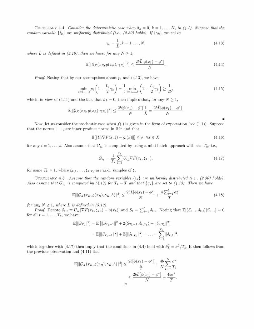
Corollary 4.4. Consider the deterministic case when σk = 0, k = 1, . . . , N , in (4.4). Suppose that therandom variable {ik} are uniformly distributed (i.e., (2.30) holds). If {γk} are set to

γk =1

L, k = 1, . . . , N, (4.13)

where L is defined in (3.10), then we have, for any N ≥ 1,

E[‖GX(xR, g(xR), γR)‖2] ≤ 2bL[φ(x1)− φ∗]N

. (4.14)

Proof. Noting that by our assumptions about pi and (4.13), we have

mini=1,...,b

pi

(1− Li

2γk

)=

1

bmin

i=1,...,b

(1− Li

2γk

)≥ 1

2b, (4.15)

which, in view of (4.11) and the fact that σk = 0, then implies that, for any N ≥ 1,

E[‖GX(xR, g(xR), γR)‖2] ≤ 2b[φ(x1)− φ∗]N

1

L=

2bL[φ(x1)− φ∗]N

.

Now, let us consider the stochastic case when f(·) is given in the form of expectation (see (1.1)). Supposethat the norms ‖ · ‖i are inner product norms in Rni and that

E[‖Ui∇F (x, ξ)− gi(x)‖] ≤ σ ∀x ∈ X (4.16)

for any i = 1, . . . , b. Also assume that Gik is computed by using a mini-batch approach with size Tk, i.e.,

Gik =1

Tk

Tk∑t=1

Uik∇F (xk, ξk,t), (4.17)

for some Tk ≥ 1, where ξk,1, . . . , ξk,Tkare i.i.d. samples of ξ.

Corollary 4.5. Assume that the random variables {ik} are uniformly distributed (i.e., (2.30) holds).Also assume that Gik is computed by (4.17) for Tk = T and that {γk} are set to (4.13). Then we have

E[‖GX(xR, g(xR), γR, h)‖2] ≤ 2bL[φ(x1)− φ∗]N

+4∑bi=1 σ

2i

T(4.18)

for any N ≥ 1, where L is defined in (3.10).Proof. Denote δk,t ≡ Uik [∇F (xk, ξk,t) − g(xk)] and St =

∑ti=1 δk,i. Noting that E[〈St−1, δk,t〉|St−1] = 0

for all t = 1, . . . , Tk, we have

E[‖STk‖2] = E

[‖STk−1‖2 + 2〈STk−1, δk,Tk

〉+ ‖δk,Tk‖2]

= E[‖STk−1‖2] + E[‖δk,Tk‖2] = . . . =

Tk∑t=1

‖δk,t‖2,

which together with (4.17) then imply that the conditions in (4.4) hold with σ2k = σ2/Tk. It then follows from

the previous observation and (4.11) that

E[‖GX(xR, g(xR), γR, h)‖2] ≤ 2b[φ(x1)− φ∗]NL

+4b

N

N∑k=1

σ2

Tk

≤ 2bL[φ(x1)− φ∗]N

+4bσ2

T.

24

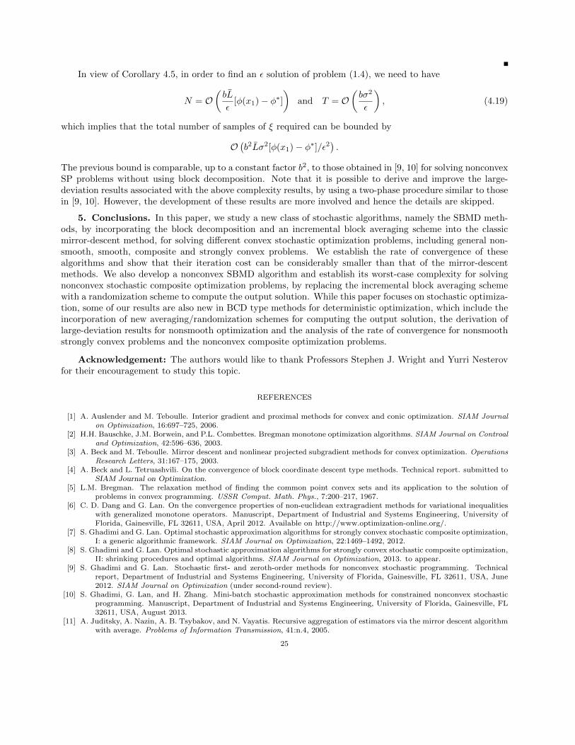
In view of Corollary 4.5, in order to find an ε solution of problem (1.4), we need to have

N = O(bL

ε[φ(x1)− φ∗]

)and T = O

(bσ2

ε

), (4.19)

which implies that the total number of samples of ξ required can be bounded by

O(b2Lσ2[φ(x1)− φ∗]/ε2

).

The previous bound is comparable, up to a constant factor b2, to those obtained in [9, 10] for solving nonconvexSP problems without using block decomposition. Note that it is possible to derive and improve the large-deviation results associated with the above complexity results, by using a two-phase procedure similar to thosein [9, 10]. However, the development of these results are more involved and hence the details are skipped.

5. Conclusions. In this paper, we study a new class of stochastic algorithms, namely the SBMD meth-ods, by incorporating the block decomposition and an incremental block averaging scheme into the classicmirror-descent method, for solving different convex stochastic optimization problems, including general non-smooth, smooth, composite and strongly convex problems. We establish the rate of convergence of thesealgorithms and show that their iteration cost can be considerably smaller than that of the mirror-descentmethods. We also develop a nonconvex SBMD algorithm and establish its worst-case complexity for solvingnonconvex stochastic composite optimization problems, by replacing the incremental block averaging schemewith a randomization scheme to compute the output solution. While this paper focuses on stochastic optimiza-tion, some of our results are also new in BCD type methods for deterministic optimization, which include theincorporation of new averaging/randomization schemes for computing the output solution, the derivation oflarge-deviation results for nonsmooth optimization and the analysis of the rate of convergence for nonsmoothstrongly convex problems and the nonconvex composite optimization problems.

Acknowledgement: The authors would like to thank Professors Stephen J. Wright and Yurri Nesterovfor their encouragement to study this topic.

REFERENCES

[1] A. Auslender and M. Teboulle. Interior gradient and proximal methods for convex and conic optimization. SIAM Journalon Optimization, 16:697–725, 2006.

[2] H.H. Bauschke, J.M. Borwein, and P.L. Combettes. Bregman monotone optimization algorithms. SIAM Journal on Controaland Optimization, 42:596–636, 2003.

[3] A. Beck and M. Teboulle. Mirror descent and nonlinear projected subgradient methods for convex optimization. OperationsResearch Letters, 31:167–175, 2003.

[4] A. Beck and L. Tetruashvili. On the convergence of block coordinate descent type methods. Technical report. submitted toSIAM Journal on Optimization.

[5] L.M. Bregman. The relaxation method of finding the common point convex sets and its application to the solution ofproblems in convex programming. USSR Comput. Math. Phys., 7:200–217, 1967.

[6] C. D. Dang and G. Lan. On the convergence properties of non-euclidean extragradient methods for variational inequalitieswith generalized monotone operators. Manuscript, Department of Industrial and Systems Engineering, University ofFlorida, Gainesville, FL 32611, USA, April 2012. Available on http://www.optimization-online.org/.

[7] S. Ghadimi and G. Lan. Optimal stochastic approximation algorithms for strongly convex stochastic composite optimization,I: a generic algorithmic framework. SIAM Journal on Optimization, 22:1469–1492, 2012.

[8] S. Ghadimi and G. Lan. Optimal stochastic approximation algorithms for strongly convex stochastic composite optimization,II: shrinking procedures and optimal algorithms. SIAM Journal on Optimization, 2013. to appear.

[9] S. Ghadimi and G. Lan. Stochastic first- and zeroth-order methods for nonconvex stochastic programming. Technicalreport, Department of Industrial and Systems Engineering, University of Florida, Gainesville, FL 32611, USA, June2012. SIAM Journal on Optimization (under second-round review).

[10] S. Ghadimi, G. Lan, and H. Zhang. Mini-batch stochastic approximation methods for constrained nonconvex stochasticprogramming. Manuscript, Department of Industrial and Systems Engineering, University of Florida, Gainesville, FL32611, USA, August 2013.

[11] A. Juditsky, A. Nazin, A. B. Tsybakov, and N. Vayatis. Recursive aggregation of estimators via the mirror descent algorithmwith average. Problems of Information Transmission, 41:n.4, 2005.

25

[12] A. Juditsky and Y. E. Nesterov. Primal-dual subgradient methods for minimizing uniformly convex functions. Manuscript.[13] A. Juditsky, P. Rigollet, and A. B. Tsybakov. Learning by mirror averaging. Annals of Statistics, 36:2183–2206, 2008.[14] G. Lan. An optimal method for stochastic composite optimization. Mathematical Programming, 133(1):365–397, 2012.[15] G. Lan. Bundle-level type methods uniformly optimal for smooth and non-smooth convex optimization. Manuscript,

Department of Industrial and Systems Engineering, University of Florida, Gainesville, FL 32611, USA, January 2013.Revision submitted to Mathematical Programming.

[16] G. Lan and R. D. C. Monteiro. Iteration-complexity of first-order penalty methods for convex programming. MathematicalProgramming, 138:115–139, 2013.

[17] G. Lan and R. D. C. Monteiro. Iteration-complexity of first-order augmented lagrangian methods for convex programming.Manuscript, School of Industrial and Systems Engineering, Georgia Institute of Technology, Atlanta, GA 30332, USA,May 2009. Mathematical Programming (under revision).

[18] G. Lan, A. S. Nemirovski, and A. Shapiro. Validation analysis of mirror descent stochastic approximation method. Mathe-matical Programming, 134:425–458, 2012.

[19] D. Leventhal and A. S. Lewis. Randomized methods for linear constraints: Convergence rates and conditioning. Mathematicsof Operations Research, 35:641–654, 2010.

[20] Q. Lin, X. Chen, and J. Pena. A sparsity preserving stochastic gradient method for composite optimization. Manuscript,Carnegie Mellon University, PA 15213, April 2011.

[21] Z. Lu and L. Xiao. On the complexity analysis of randomized block-coordinate descent methods. Manuscript, 2013.[22] Z.Q. Luo and P. Tseng. On the convergence of a matrix splitting algorithm for the symmetric monotone linear complemen-

tarity problem. SIAM Journal on Control and Optimization, 29:037 – 1060, 1991.[23] A. Nedic. On stochastic subgradient mirror-descent algorithm with weighted averaging. 2012.[24] A. S. Nemirovski, A. Juditsky, G. Lan, and A. Shapiro. Robust stochastic approximation approach to stochastic program-

ming. SIAM Journal on Optimization, 19:1574–1609, 2009.[25] A. S. Nemirovski and D. Yudin. Problem complexity and method efficiency in optimization. Wiley-Interscience Series in

Discrete Mathematics. John Wiley, XV, 1983.[26] Y. E. Nesterov. Introductory Lectures on Convex Optimization: a basic course. Kluwer Academic Publishers, Massachusetts,

2004.[27] Y. E. Nesterov. Primal-dual subgradient methods for convex problems. Mathematical Programming, 120:221–259, 2006.[28] Y. E. Nesterov. Efficiency of coordinate descent methods on huge-scale optimization problems. Technical report, Center for

Operations Research and Econometrics (CORE), Catholic University of Louvain, Feburary 2010.[29] Y. E. Nesterov. Subgradient methods for huge-scale optimization problems. Technical report, Center for Operations Research

and Econometrics (CORE), Catholic University of Louvain, Feburary 2012.[30] F. Niu, B. Recht, C. Re, and S. J. Wright. Hogwild!: A lock-free approach to parallelizing stochastic gradient descent.

Manuscript, Computer Sciences Department, University of Wisconsin-Madison, 1210 W Dayton St, Madison, WI 53706,2011.

[31] B.T. Polyak. New stochastic approximation type procedures. Automat. i Telemekh., 7:98–107, 1990.[32] B.T. Polyak and A.B. Juditsky. Acceleration of stochastic approximation by averaging. SIAM J. Control and Optimization,

30:838–855, 1992.[33] P. Richtarik and M. Takac. Iteration complexity of randomized block-coordinate descent methods for minimizing a composite

function. Mathematical Programming, 2012. to appear.[34] H. Robbins and S. Monro. A stochastic approximation method. Annals of Mathematical Statistics, 22:400–407, 1951.[35] S. Shalev-Shwartz and A. Tewari. Stochastic methods for l1 regularized loss minimization. Manuscript, 2011. Submitted to

Journal of Machine Learning Research.[36] A. Shapiro, D. Dentcheva, and A. Ruszczynski. Lectures on Stochastic Programming: Modeling and Theory. SIAM,

Philadelphia, 2009.[37] M. Teboulle. Convergence of proximal-like algorithms. SIAM Journal on Optimization, 7:1069–1083, 1997.[38] P. Tseng. Convergence of a block coordinate descent method for nondifferentiable minimization. Journal of Optimization

Theory and Applications, 109:475494, 2001.[39] P. Tseng and S. Yun. A coordinate gradient descent method for nonsmooth separable minimization. Mathematical Pro-

gramming, 117:387–423, 2009.[40] S. J. Wright. Accelerated block-coordinate relaxation for regularized optimizations. Manuscript, University of Wisconsin-

Madison, Madison, WI, 2010.[41] L. Xiao. Dual averaging methods for regularized stochastic learning and online optimization. J. Mach. Learn. Res., pages

2543–2596, 2010.[42] E. P. Xing, A. Y. Ng, M. I. Jordan, and S. Russell. Distance metric learning, with application to clustering with side-

information. In Advances in Neural Information Processing Systems 15, pages 505–512. MIT Press, 2002.

26