stochastic characterization of the two band two player
TRANSCRIPT

HAL Id: hal-00766448https://hal.inria.fr/hal-00766448
Submitted on 18 Dec 2012
HAL is a multi-disciplinary open accessarchive for the deposit and dissemination of sci-entific research documents, whether they are pub-lished or not. The documents may come fromteaching and research institutions in France orabroad, or from public or private research centers.
L’archive ouverte pluridisciplinaire HAL, estdestinée au dépôt et à la diffusion de documentsscientifiques de niveau recherche, publiés ou non,émanant des établissements d’enseignement et derecherche français ou étrangers, des laboratoirespublics ou privés.
Stochastic characterization of the two band two playerspectrum sharing game
Ilaria Malanchini, Steven Weber, Matteo Cesana
To cite this version:Ilaria Malanchini, Steven Weber, Matteo Cesana. Stochastic characterization of the two band twoplayer spectrum sharing game. WiOpt’12: Modeling and Optimization in Mobile, Ad Hoc, andWireless Networks, May 2012, Paderborn, Germany. pp.343-348. �hal-00766448�

Stochastic characterization of the two band two
player spectrum sharing game
Ilaria Malanchini∗†, Steven Weber† and Matteo Cesana∗
∗ Politecnico di Milano, DEI† Drexel University, Dept. of ECE
Email: [email protected], [email protected], [email protected]
Abstract—We consider two pairs of communicating users shar-ing two bands of spectrum under a sum band power constraint.Our earlier work proposed a natural spectrum sharing gamefor this problem and characterized the Nash equilibria as afunction of the signal and interference distances, when thepositions of the four nodes were assumed fixed. In this work,we derive i) the joint distribution of the interference distancesconditioned on the transmitter separation distance, as well asii) the unconditioned interference distance distribution when weplace one transmitter at the origin and the second uniformly atrandom over a disk. This allows us to compute the distributionof the random Nash equilibria and random prices of anarchyand stability as a function of the random interference distances.We leverage the analysis to give an asymptotic expression for thecoupling probability in a game where the transmitter positionsform a (low density) Poisson process, which may be interpretedas the fraction of players essentially playing a two player game.
I. INTRODUCTION
In this paper, we analyze the dynamics among multiple
pairs of users that want to communicate sharing the same
portion of the spectrum. We model this interaction using
game theory, since, in general, the quality perceived by a
user strictly depends on the behavior of other entities. We
consider a Gaussian Interference Game (GIG) [1], where two
transmitter and receiver pairs have to decide how to split the
total power budget P across two orthogonal channels of the
spectrum with equal bandwidths B, maximizing the sum of the
Shannon rate achieved on each band. Non–cooperative game
theory is suitable in distributed networks, where control and
management are decentralized. For this reason, we model the
problem as a non–cooperative game, in which selfish users
aim to maximize their achieved throughput.
In our previous work [2], the game is characterized an-
alytically assuming that the positions of the two transmit-
ter/receiver couples are known. In this scenario, we derive
the quality/number of the Nash equilibria, highlighting the
dependence on the parameters that define the topology (in-
terference distances x1, x2 and signal distance d) and the
propagation model (pathloss exponent α and noise power η).
Since the wireless network performance is strongly influenced
by the spatial distribution of the communicating/interfering
nodes, a natural objective is to analyze the dependence of the
equilibria distribution on the node positions. Therefore, we fix
one transmitter at the origin and place the second transmitter
uniformly at random in a disk of radius L. The two receivers
are placed uniformly at random along the circles of radius d
centered at the corresponding transmitter. Basic stochastic
geometry is used to characterize the joint distribution of the
interference distances x1, x2, and to compute the distribution
of the random equilibria.
The stochastic characterization of the 2–player game can be
leveraged as a starting point to tackle the more general N–
player game. Namely, the analysis of large networks game
can be simplified, identifying couples of pairs in the N–
player game that play small 2–player sub–games. The key
result of this paper is to provide, for the low–density regime,
the fraction of nodes whose game can be characterized using
the stochastic analysis of the 2–player game. The complete
analysis of the N–player game is part of the ongoing work and
the results of this paper are fundamental in order to assess the
network performance of large networks with game theoretic
dynamics.
The paper is organized as follows: §II reviews prior work
on spectrum sharing games; §III sets the reference scenario
and recalls previous results for the spectrum sharing game;
§IV provides a stochastic analysis of the 2–player game; and
§V shows how these results can be used to evaluate the
performance in large N–player networks.
II. RELATED WORK
Spectrum sharing games have been widely studied in the
literature. In [1], the authors propose a spectrum sharing game
for multiple players that share the same portion of spectrum.
In particular, they introduce self-enforcing rules that allow
users to reach an efficient and fair solution. In [3], the authors
consider a power control problem with SINR as objective
function, in both the selfish and the cooperative scenario. In
contrast, non–cooperative games among operators that share
the spectrum are proposed in [4] and [5]. Both these papers
characterize the Nash equilibria of the system. Games based
on the water–filling algorithm are proposed in [6] and [7]. The
authors consider a scenario composed by two contending com-
municating systems and study the existence and uniqueness
of the Nash equilibrium. The water–filling algorithm is used
also in [8] and [9]. A unified view of main results presented
in the literature is proposed in [10]. This work shows how
the different approaches proposed in the literature can be
unified following a unique interpretation of the waterfilling
solution. Furthermore, a unified set of sufficient conditions
that guarantee the uniqueness of the equilibrium is derived.
8th International Workshop on Spatial Stochastic Models for Wireless Networks, 14 May 2012
978-1-61284-824-2/2012 - Copyright is with IFIP 343

Power control games in the context of cognitive radio
networks are considered in [11] and [12]. Existence and
properties of the Nash equilibria are investigated assuming
the interference temperature model. Furthermore, the channel
competition is studied in [13] and [14]. The authors charac-
terize the equilbria of the game and assess their quality with
respect to the optimal solution. In [15], the power allocation
game is modeled as a potential game that is shown to possess
a unique equilibrium. When the channels are assumed to
fluctuate stochastically over time, stochastic approximation
theory is used to show convergence to equilibrium.
There exist other few works that propose a stochastic anal-
ysis of games in the context of wireless networks. In [16], the
authors propose a stochastic game that models the interactions
among users that compete for the available spectrum opportu-
nities. In particular, users make bids for the required resources.
A best–response algorithm is proposed in order to improve the
users’ bidding policy. A random access game is proposed also
in [17], where the authors characterize the Nash equilibria of
the random access game and analyze the asymptotic properties
of the system as the number of users goes to infinity. [18]
provides a useful tutorial on different techniques based on
stochastic geometry and the theory of random geometric
graphs. Different from previous work, we introduce the use
of stochastic geometry in order to characterize the equilibria
of the game in terms of probability distribution over the set
of possible equilibria.
III. REFERENCE SCENARIO
We consider the spectrum sharing game, where two trans-
mitter and receiver pairs (the players) have to decide how
to split the total power budgets over two available bands
(the actions), maximizing the sum of the achievable Shannon
rates over the two bands (the payoffs). Namely, the reference
topology is reported in Fig. 1. We label the distance between
the two transmitters t and assume that the corresponding
receivers are placed uniformly around the transmitters at a
fixed distance d, i.e., a and b are uniform angles in the range
[0, 2π]. (Note that in this section we assume a and b to be fixed,
whereas we will treat them as random variables in the next
section.) Let x1 and x2 be the distance between receiver 1and transmitter 2 and the distance between receiver 2 and
transmitter 1, respectively. The strategy space of the generic
transmitter i is Pi ∈ [0, 1]. Namely, Pi is the fraction of Pthat pair i uses in the left band and Pi = 1 − Pi is the
fraction of power in the right band. The utility function of
each player is defined as the sum achievable Shannon rate over
the two bands when the interference from the other player
is treated as noise. We assume a channel model with pure
pathloss attenuation, where α > 2 is the pathloss exponent.
Assuming a noise power of η on each band, the utility function
of player 1 (and symmetrically of player 2) for transmission
powers P ≡ (P1, P2) ∈ [0, 1]2 is:
U1(P ) = log2
(
1 +P1d
−α
η + P2x−α1
)
+log2
(
1 +P1d
−α
η + P2x−α1
)
.
(1)
Fig. 1. 2–player topology.
The characterization of pure Nash equilibria derived in [2] is
reported in Fig. 2, where β±i = 0.5
(
1± x−αi /d−α
)
. Note that
there exist four regions. When x1x2 < d2, the game admits
three equilibria and the optimum is in (0, 1) and (1, 0). In
particular, when both x1 and x2 are smaller than d, the PoS is
one, since the best equilibrium and the optimum coincide. In
contrast, when x1 (or x2) is greater than d, the best equilibrium
is worse than the optimum, then the PoS is greater than one.
The PoA is in both the two cases greater than one. When
x1x2 > d2 and x−α1 x−α
2 + ηx−α1 + ηx−α
2 − ηd−α < 0 the
game admits a unique equilibrium, that does not coincide with
the optimum, then PoS and PoA coincide and are greater than
one. In contrast, when
x−α1 x−α
2 + ηx−α1 + ηx−α
2 − ηd−α > 0 (2)
the optimal solution and the unique equilibrium coincide.
Finally, along the curve x1x2 = d2 the two best responses
coincide and there exists an infinite number of equilibria.
Fig. 2. Nash equilibria and optimal allocations as a function of x1 and x2
(for d = 25).
From this analysis, we can conclude that the equilibrium
chosen by the two players (as well as the correspond-
ing PoS/PoA) depends upon the two interference distances
(x1, x2). When node positions are random, it follows that
(x1, x2) are random, and thus the equilibrium is random. In
short, we compute probabilities of being in the various regions
in Fig. 2.
344

IV. STOCHASTIC ANALYSIS OF THE 2–PLAYER GAME
We use standard probabilistic notation: sans-serif letters
(e.g., x) denote random variables (RV) and italic characters
denote their corresponding value (e.g., x). The cumulative
distribution function (cdf), its complement (ccdf), and prob-
ability density function (pdf) are denoted Fx(x), Fx(x) =1 − Fx(x), fx(x), respectively, with the natural notational
extensions for conditional and joint distributions.
A. Conditional joint pdf of the interference distances
We suppose the two transmitters are placed at random and
we condition on the distance separating them t. We further
suppose each receiver is placed uniformly at random on the
circle of radius d centered at the corresponding transmitter. It
follows that the interference distances x1, x2 are conditionally
independent given t:
Fx1,x2|t(x1, x2|t) ≡ P(x1 ≤ x1, x2 ≤ x2|t) == P(x1 ≤ x1|t)P(x2 ≤ x2|t). (3)
Using the law of cosines x21 = d2 + t2 − 2dt cos a:
P(x1 ≤ x1|t) = P(d2 + t2 − 2dt cos a ≤ x21|t) =
= P
(
cos a ≥ (d2 + t2)− x21
2dt
∣
∣
∣
∣
t
)
. (4)
The following proposition is elementary.
Proposition IV.1. The random variable w, cosine of a uni-
formly distributed angle, has the following distribution:
fw(w) =1
π√1− w2
, Fw(w) =1
2+
1
πsin−1 w, w ∈ [−1, 1].
Using this result, we can now state the following theorem.
Theorem IV.2. The joint cdf and pdf of x1, x2 conditioned
on t are given by Eq. (5) and Eq. (6) (reported on page 4),
respectively, where Fw(w) is given in Prop. IV.1.
Proof: For the sake of brevity, we only report some
mathematical steps. From Eq. (4) and Prop. IV.1:
P
(
cos a ≥ (d2 + t2)− x21
2dt
∣
∣
∣
∣
t
)
= Fw
(
(d2 + t2)− x21
2dt
∣
∣
∣
∣
t
)
.
(7)
From Eq. (3):
Fx1,x2|t(x1, x2|t)=Fw
(
(d2 + t2)− x21
2dt
)
Fw
(
(d2 + t2)− x22
2dt
)
.
(8)
Eq. (5) follows by requiring the argument of the cdf Fw(w)to be between −1 and 1. Eq. (6) follows directly from taking
the double partial derivative with respect to x1 and x2:
fx1,x2|t(x1, x2|t) =∂2
∂x1∂x2Fx1,x2|t(x1, x2|t). (9)
Fig. 3 shows the conditional joint pdf and cdf when d = 1and t = 3. Note that we obtain a function different from zero
only in the region {(x1, x2) : |d − t| ≤ x1 ≤ d + t, |d −t| ≤ x2 ≤ d + t}, consistent with the topology constraints
mentioned at the beginning of this section.
B. Joint pdf of the mutual interference distances
For any distribution on the random distance t separating the
transmitters, we obtain the joint (unconditioned) distribution
for (x1, x2) by the total probability theorem:
fx1,x2(x1, x2) =
∫ ∞
0
fx1,x2|t(x1, x2|t)ft(t)dt. (10)
We will henceforth assume the random transmitter separation
distance t is determined by placing one of the transmitters
at the origin of a disk of radius L, and placing the second
transmitter uniformly at random in the disk. We emphasize,
however, that Eq. (10) holds for any distribution on t, and our
assumption is merely for the purpose of concreteness. Under
this assumption, the RV t has cdf and pdf:
Ft(t) =
(
t
L
)2
, ft(t) =2t
L2, 0 ≤ t ≤ L. (11)
The RVs x1, x2 are not (unconditionally) independent. Due to
the geometry of the problem (the sum of any two sides of
a triangle must be greater than the third side), the following
inequalities must hold:
|d− t| ≤ x1 ≤ d+ t (12)
|d− t| ≤ x2 ≤ d+ t
max{|d− x1|, |d− x2|} ≤ t ≤ min{d+ x1, d+ x2}We can now state the following theorem.
Theorem IV.3. Suppose the distance t between the two
transmitters has the distribution in Eq. (11). Then the joint
pdf of x1, x2 is given by Eq. (13) (reported on page 5) and the
support of (x1, x2) is given by Eq. (12).
Proof: Substitute Eq. (11) for ft(t) and Eq. (6) for
fx1,x2|t(x1, x2|t) in Eq. (10), using the constraints in Eq. (12).
Note that, in general, it is not possible to provide close form
expression of the integral in Eq. (13). Numerical evaluation,
however, is straightforward.
C. Distribution on the Nash equilibria
We can now use the joint distribution in Thm. IV.3 to
compute the distribution of the equilibria in Fig. 2. Each
equilibria’s probability can be evaluated via:∫
P
fx1,x2(x1, x2)dx1dx2 (14)
where P is the set of points that defines that region. Table I
summaries the different cases, which are illustrated in Fig. 4.
Namely, unique refers to the probability that the equilibrium is
unique. When the equilibrium is not unique, we consider two
cases. The case in which the three equilibria are (0.5, 0.5),(0, 1) and (1, 0), i.e., (0.5,0.5)-(0,1)-(1,0), and the case in
which the equilibria depend on the parameter β, (mixed). For
completeness, we also provide the probability that there is
an infinite number of equilibria (infinite). Finally, we evaluate
the probability that the unique equilibrium and the optimal
solution coincide (coincide w/opt).
345

Fx1,x2|t(x1, x2|t) =
=
0 x1 < |d− t| or x2 < |d− t|[
1− Fw
(
(d2+t2)−x21
2dt
)] [
1− Fw
(
(d2+t2)−x22
2dt
)]
|d− t| ≤ x1 ≤ d+ t and |d− t| ≤ x2 ≤ d+ t[
1− Fw
(
(d2+t2)−x21
2dt
)]
|d− t| ≤ x1 ≤ d+ t and x2 > d+ t[
1− Fw
(
(d2+t2)−x22
2dt
)]
x1 > d+ t and |d− t| ≤ x2 ≤ d+ t
1 x1 > d+ t and x2 > d+ t
(5)
fx1,x2|t(x1, x2|t) =
=
x1x2
π2d2t2
√
[
1−
(
d2+t2−x21
2dt
)
2][
1−
(
d2+t2−x22
2dt
)
2]
|d− t| ≤ x1 ≤ d+ t and |d− t| ≤ x2 ≤ d+ t
0 else
(6)
Fig. 3. Conditional joint pdf (left) and cdf (right) of x1 and x2 when d = 1and t = 3.
TABLE IDIFFERENT EVENTS THAT ARE CONSIDERED IN THE STOCHASTIC
ANALYSIS OF THE GAME.
“event” P
unique x1x2 > d2
(0.5,0.5)-(0,1)-(1,0) x1 < d ∧ x2 < d
mixed x1x2 < d2 ∧ (x1 > d ∨ x2 > d)infinite x1x2 = d2
coincide w/opt (x1x2)−α + η(x−α
1+ x−α
2− d−α) > 0
Numerical results for all these probabilities are reported in
Fig. 5. We consider four different values of d, with L varying
from 0.1 to 50. We assume η = 10−3 and α = 4. Clearly, the
probability of having a unique equilibrium, that corresponds
to the case in which players decide to use the whole spectrum,
increases with L. This is reasonable since increasing L, also
the average distance between the interfering pairs increases
(x1 and x2), then, for a fixed d, the probability of x1x2 > d2
increases. This corresponds to the case in which users share
the same spectrum since the interfere is small. In particular, we
can see that when L < d that probability is around 50% and
then starts increasing, approaching 1 when L ≃ 5d. Note that
the probability of having an infinite number of Nash equilibria
is very close to zero, as expected (sometimes it is slightly
different from zero for numerical issues in the evaluation of
the integral). Furthermore, the probability that the optimum
and the unique equilibrium coincide has a similar behavior of
the probability of uniqueness, but it is lower. This is obvious,
since when the equilibrium and the optimum coincide, the
equilibrium is also unique, but the opposite is not always true.
Moreover, when L = 0, the two transmitters coincide, then
x1 = x2 = d, that corresponds to the case in which there exists
an infinite number of Nash equilibria. In contrast, when L = ǫ,for any small ǫ > 0, each x can be a little bit greater or a little
bit smaller than d (remember that x2 = d2 + ǫ2 − 2dǫ cos a).
We can see this in Fig. 6 (left).
In particular, the zoom reported in Fig. 6 (right) explains
why when L approaches zero, the probability of unique
equilibrium is equal to 0.5 (given by the probability that both
the xs are greater than d). Therefore, also the probability of
having three equilibria is 0.5. In particular, this is half split
between having {(0, 1), (1, 0), (0.5, 0.5)} (both x’s are less
than d and this happens with probability 0.25) and the mixed
case (when only one x is greater than d, but both below the
curve x1x2 = d2).
Finally, note that when L goes to zero the optimum never
coincides with the equilibrium in (0.5, 0.5). In fact, the optimal
solution always corresponds to split and use different portions
of the spectrum. The reason why, when L = ǫ, with ǫ small,
this probability approaches zero is clear also from Fig. 6
(right). In fact, when L = ǫ, the two x’s are both close to dand they do not satisfy the condition given by Eq. (2).
V. COUPLING PROBABILITY
In the previous section we provided a stochastic character-
ization of the 2–player game. We now illustrate the value of
this analysis in the corresponding N -player game. Consider
the Binomial Point Process (BPP) ΠN = {u1, . . . , uN} where
N transmitters are positioned independently and uniformly
at random in a compact set A ⊂ R2 with N/|A| = λ; we
refer to λ as the density. The N receivers {v1, . . . , vN} are
each positioned independently and uniformly at random on the
circle of radius d centered at the corresponding transmitter.
The sum and maximum (shot noise) interference processes
seen at receiver vj under BPP ΠN are:
ΣΠN(vj) ≡
∑
ui∈ΠN\{uj}
‖ui−vj‖−α, MΠN(vj) ≡ max
ui∈ΠN\{uj}‖ui−vj‖−α.
(15)
346

fx1,x2(x1, x2) =2x1x2
π2d2L2
∫ min{d+x1,d+x2}
max{|d−x1|,|d−x2|}
1
t
√
[
1−(
d2+t2−x21
2dt
)2] [
1−(
d2+t2−x22
2dt
)2]
dt. (13)
unique (0.5,0.5)-(0,1)-(1,0)
mixed coincide w/opt
Fig. 4. Regions of Fig. 2 that we are considering in Table I .
As discussed in [19] (§2.5), the sum interference RV Σ is
subexponential, meaning
limz→∞
P(ΣΠN(vj) > z)
P(MΠN(vj) > z)
= 1. (16)
That is, the sum interference is large when the maximum
interference term is large, i.e., intuitively approximating the
sum interference by the maximum is a valid approximation.
The key insight is that under the approximation Σ ≈ M
the N -player game will decouple into subgames, described in
what follows. We introduce the following definition:
Definition V.1 (Coupled users). Users (ui, vi) and (uj , vj) are
coupled if the nearest interfering transmitter of receiver vj is
ui and the nearest interfering transmitter of receiver vi is uj .
Under the approximation Σ ≈ M, a pair of coupled users in
the N–player game are playing a 2–player game. We define
the probability of a typical user being coupled:
Definition V.2 (Coupling probability). The coupling probabil-
ity Pc(λ) is the probability that a typical user, say (ui, vi), is
coupled with the user whose transmitter, say uj , is the closest
interferer to vi, i.e., the probability that ui is in fact also the
closest interferer to vj:
Pc(λ) = P(i = argmink 6=j
‖uk − vj‖ | j = argmink 6=i
‖uk − vi‖).(17)
Refer to Fig. 1. Assume that TX2 is the nearest interferer
for RX1. Note that this means that there is no other transmitter
in the circle (say, C1) of radius x1 with center RX1, i.e.,
ΠN (C1) = 0. The probability that TX1 is the nearest interferer
for RX2 is Pc(λ) = P(ΠN (C2) = 0|ΠN (C1) = 0), where
C2 is the circle of radius x2 with center RX2. Although
occupancy counts of disjoint regions are dependent in a BPP,
the dependence vanishes in the limit as the BPP becomes
a Poisson Point Process (PPP), i.e., as N, |A| → ∞ with
N/|A| → λ. Under this approximation we have
Pc(λ) ≈ P(Πλ(∆) = 0) = e−λ|∆|, (18)
i.e., the coupling probability is approximately the void proba-
bility for a PPP Πλ of intensity λ on the lune ∆ ≡ C2 \ C1.
Theorem V.3. The value for the coupling probability when λgoes to 0 is the following constant:
limλ→0
Pc(λ) = Ccp ,6π
3√3 + 8π
≈ 0.6215.
Proof: In the low density (small λ) regime the BPP
behaves like the PPP since |A| must be large. Recall that the
average distance to a nearest neighbor in a PPP with density
λ is 1/√λ, and thus for small λ the average distance is large.
To obtain the value of the coupling probability in the low
density regime, we can assume that x1 ≫ d and x2 ≫ d.
Thus as λ → 0, d can be neglected and we can assume that
x1 = x2. In this scenario, reported in Fig. 7, we have two
circles with the same radius, whose centers are separated by
a distance equal to the radius itself. Therefore, the area of the
lune depends only on the parameter x1. In particular, using
the formula of the area of the lune, we obtain that in this case
the area of the lune is the following:
∆ =
(
π
3+
√3
2
)
x21. (19)
Applying the total probability theorem:
Pc(λ) =
∫ ∞
0
Pc|x1(λ, x1)fx1(x1)dx1. (20)
The distribution of the nearest interferer is:
fx1(x1) = 2πλx1e−πλx2
1 x1 ≥ 0. (21)
Substituting the expression for fx1(x1) in Eq. (21) and the
void probability over the area in Eq. (19), we obtain:
Pc(λ) =
∫ ∞
0
e−λ
(
π3+
√
3
2
)
x212πλx1e
−πλx21dx1 = Ccp. (22)
Fig. 8 reports different curves for the coupling probability
Pc(λ) vs. λ. The black point is Ccp. Thus, in the low density
regime, under approximation that the sum interference equals
the max interference, 62% of the nodes play a 2–player game,
for which the analysis in §IV applies. Note the sum/max
347
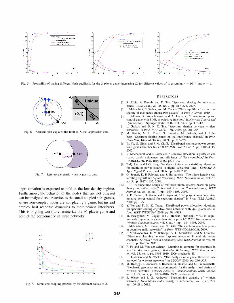
Fig. 5. Probability of having different Nash equilibria for the 2–player game, increasing L, for different values of d, assuming η = 10−3 and α = 4.
Fig. 6. Scenario that explains the limit as L that approaches zero.
Fig. 7. Reference scenario when λ goes to zero.
approximation is expected to hold in the low density regime.
Furthermore, the behavior of the nodes that are not coupled
can be analyzed as a reaction to the small coupled sub–games,
where non-coupled nodes are not playing a game, but instead
employ best response dynamics to their nearest interferers.
This is ongoing work to characterize the N–player game and
predict the performance in large networks.
Fig. 8. Simulated coupling probability for different values of d.
REFERENCES
[1] R. Etkin, A. Parekh, and D. Tse, “Spectrum sharing for unlicensedbands,” IEEE JSAC, vol. 25, no. 3, pp. 517–528, 2007.
[2] I. Malanchini, S. Weber, and M. Cesana, “Nash equilibria for spectrumsharing of two bands among two players,” in Proc. Allerton, 2010.
[3] E. Altman, K. Avrachenkov, and A. Garnaev, “Transmission powercontrol game with SINR as objective function,” in Network Control and
Optimization. Springer Berlin, 2009, vol. 5425, pp. 112–120.[4] L. Grokop and D. N. C. Tse, “Spectrum sharing between wireless
networks,” in Proc. IEEE INFOCOM, 2008, pp. 201–205.[5] M. Bennis, M. L. Treust, S. Lasaulce, M. Debbah, and J. Lille-
berg, “Spectrum sharing games on the interference channel,” in Proc.
GameNets, Istanbul, Turkey, 2009, pp. 515–522.[6] W. Yu, G. Ginis, and J. M. Cioffi, “Distributed multiuser power control
for digital subscriber lines,” IEEE JSAC, vol. 20, no. 5, pp. 1105–1115,2002.
[7] R. Mochaourab and E. Jorswieck, “Resource allocation in protected andshared bands: uniqueness and efficiency of Nash equilibria,” in Proc.
GAMECOMM, Pisa, Italy, 2009, pp. 1–10.[8] Z.-Q. Luo and J.-S. Pang, “Analysis of iterative waterfilling algorithm
for multiuser power control in digital subscriber lines,” EURASIP J.
Appl. Signal Process., vol. 2006, pp. 1–10, 2005.[9] G. Scutari, D. P. Palomar, and S. Barbarossa, “The mimo iterative wa-
terfilling algorithm,” Signal Processing, IEEE Transactions on, vol. 57,no. 5, pp. 1917–1935, 2009.
[10] ——, “Competitive design of multiuser mimo systems based on gametheory: A unified view,” Selected Areas in Communications, IEEE
Journal on, vol. 26, no. 7, pp. 1089–1103, 2008.[11] R. D. Taranto, H. Yomo, and P. Popovski, “Two players non-cooperative
iterative power control for spectrum sharing,” in Proc. IEEE PIMRC,2008, pp. 1–5.
[12] Y. Wu and D. H. K. Tsang, “Distributed power allocation algorithmfor spectrum sharing cognitive radio networks with QoS guarantee,” inProc. IEEE INFOCOM, 2009, pp. 981–989.
[13] M. Felegyhazi, M. Cagalj, and J. Hubaux, “Efficient MAC in cogni-tive radio systems: a game-theoretic approach,” IEEE Transactions on
Wireless Communications, vol. 8, no. 4, pp. 1984–1995, 2009.[14] I. Malanchini, M. Cesana, and N. Gatti, “On spectrum selection games
in cognitive radio networks,” in Proc. IEEE GLOBECOM, 2009.[15] P. Mertikopoulos, E. V. Belmega, A. L. Moustakas, and S. Lasaulce,
“Distributed learning policies forpower allocation in multiple accesschannels,” Selected Areas in Communications, IEEE Journal on, vol. 30,no. 1, pp. 96–106, 2012.
[16] F. Fu and M. Van der Schaar, “Learning to compete for resources inwireless stochastic games,” Vehicular Technology, IEEE Transactions
on, vol. 58, no. 4, pp. 1904–1919, 2009, stochastic SI.[17] H. Inaltekin and S. Wicker, “The analysis of a game theoretic mac
protocol for wireless networks,” in SECON, 2006, pp. 296–305.[18] M. Haenggi, J. Andrews, F. Baccelli, O. Dousse, and M. Franceschetti,
“Stochastic geometry and random graphs for the analysis and design ofwireless networks,” Selected Areas in Communications, IEEE Journal
on, vol. 27, no. 7, pp. 1029–1046, 2009, stochastic SI.[19] S. Weber and J. G. Andrews, “Transmission capacity of wireless
networks,” Foundations and Trends R© in Networking, vol. 5, no. 2–3,pp. 109–281, 2012.
348