stochastic k-neighborhood selection for supervised and ...dtarlow/tarswercharsutzem_icml2013.pdf ·...

Stochastic k-Neighborhood Selection for Supervised andUnsupervised Learning

Daniel Tarlow† [email protected] Research CambridgeKevin Swersky, Laurent Charlin {kswersky, lcharlin}@cs.toronto.eduUniversity of TorontoIlya Sutskever† [email protected] Inc.Richard S. Zemel [email protected] of Toronto

Abstract

Neighborhood Components Analysis (NCA)is a popular method for learning a distancemetric to be used within a k-nearest neigh-bors (kNN) classifier. A key assumption builtinto the model is that each point stochasti-cally selects a single neighbor, which makesthe model well-justified only for kNN withk = 1. However, kNN classifiers with k >1 are more robust and usually preferred inpractice. Here we present kNCA, which gen-eralizes NCA by learning distance metricsthat are appropriate for kNN with arbitraryk. The main technical contribution is show-ing how to efficiently compute and optimizethe expected accuracy of a kNN classifier. Weapply similar ideas in an unsupervised settingto yield kSNE and kt-SNE, generalizationsof Stochastic Neighbor Embedding (SNE, t-SNE) that operate on neighborhoods of sizek, which provide an axis of control over em-beddings that allow for more homogeneousand interpretable regions. Empirically, weshow that kNCA often improves classificationaccuracy over state of the art methods, pro-duces qualitative differences in the embed-dings as k is varied, and is more robust withrespect to label noise.

1. IntroductionDistance metrics are used extensively in machinelearning, both as an essential part of an algorithm likein k-means or k-nearest neighbors (kNN) algorithms,

Proceedings of the 30 th International Conference on Ma-chine Learning, Atlanta, Georgia, USA, 2013. JMLR:W&CP volume 28. Copyright 2013 by the author(s).

and as a regularizer in, e.g., semi-supervised learning.An obvious problem is that the space in which datais collected is not always suitable for the target task(e.g., nearest neighbor classification); the choice of pa-rameters like the scale of each dimension can signif-icantly impact performance of algorithms. Thus, along-standing goal is to learn the distance metric so asto maximize performance on the target task.

Neighborhood Component Analysis (NCA) is amethod that aims at doing precisely this, adapting thedistance metric to optimize a smooth approximationto the accuracy of the kNN classifier. A shortcomingof the NCA model is that it assumes k = 1, and in-deed, all of the experiments in (Goldberger et al., 2004)and many in follow-up applications are performed withk = 1. This choice appears to be made for the sake ofcomputational convenience: generalizing NCA for arbi-trary k requires computing expected accuracies over allpossible ways of choosing k neighbors from N points,which appears to be difficult when k is large. But sincekNN with k > 1 tends to perform better in practice,it seems desirable to formulate an NCA method thatdirectly optimizes the performance of kNN for k > 1.

The primary method we present, kNCA, is a strictgeneralization of NCA, which optimizes the distancemetric for expected accuracy of kNN for any choiceof k, and is equivalent to NCA when k is set to 1.The main algorithmic contribution of our work is aconstruction that allows the expected accuracy to becomputed and differentiated exactly and efficiently.We also show that similar techniques can be appliedto other problems related to the stochastic selectionof k-neighborhoods, such as is required when extend-

† Work done primarily while authors were at the Uni-versity of Toronto.

Stochastic k-Neighborhood Selection

ing Stochastic Neighbor Embedding (SNE) methodsto their k-neighbor analogs.

Thus, we make several contributions. The primarycontribution is the extension of NCA so that it is ap-propriate when we wish to use a kNN classifier at testtime with k > 1. Secondary contributions are the tech-niques for computing expected accuracy and the exten-sion of SNE to the k-neighborhood setting. We explorethe methods empirically: quantitatively, by comparingperformance to several popular baselines on a rangeof illustrative problems, and qualitatively, by visualiz-ing the learned embeddings by (supervised) kNCA and(unsupervised) kSNE.

2. BackgroundWe begin with some basic notation. Input vectors aredenoted by x ∈ RD. In supervised settings, the classlabel for a vector is denoted y ∈ {1, . . . , C}. A data setD is made up of N tuples (xi, yi)N

i=1, and X ∈ RD×N

is the concatenation of all xi as column vectors. Sim-ilarly, Y is the vector of all the labels yi. We usezi ∈ RP to represent a point in the transformed spacethat is associated with xi, and Z to represent the con-catenation of all zi as column vectors. We use [·] asthe indicator function.2.1. Neighborhood Components AnalysisAt a high level, the goal of NCA is to optimize a dis-tance metric under the objective of performance ofkNN algorithms. There are many ways to parameter-ize a distance metric, and this choice is not fundamen-tal to the approach (for example, a non-linear exten-sion like in Salakhutdinov & Hinton (2007) would bestraightforward). For simplicity, we follow NCA andframe the presentation under the assumption that thedistance between two vectors x and x′ is defined as

dA(x, x′) = (x− x′)>A>A(x− x′). (1)

This choice has the interpretation that we are first lin-early projecting points x ∈ RD into P -dimensionalspace via the matrix A ∈ RP×D, then comput-ing Euclidean distances in the P -dimensional space.NCA also gives us the ability to visualize the learnedmetric by setting P to be small and plotting trans-formed points Z = AX.

Optimizing the entries of A requires the specificationof a learning objective. A first attempt might be theaccuracy of a kNN classifier. This approach is notfeasible, because as a function of A, the performanceof a kNN classifier is a piecewise constant function,which is not possible to optimize with gradient meth-ods (note that any change in A that does not changethe neighbor set of any point will not affect this ob-jective). However, even if this approach were feasible,

we still might prefer a smooth objective for the sakeof robustness to noise in the data. For example, if apoint has a neighbor of the proper class at a distanceof b away, and many neighbors of other classes at a dis-tance of b+ε away, the kNN accuracy where k = 1 willattain the maximum objective. This clearly is not arobust solution, though, since a slight perturbation ofthe data would likely lead to an error on this example.

These considerations lead to the central NCA ideaof casting kNN in a probabilistic light. Specifically,(Goldberger et al., 2004) define a probability of select-ing each point as its 1-nearest neighbor, which is afunction of distance in transformed space. The learn-ing objective is then the expected accuracy of a 1-nearest neighbor classifier under this probability dis-tribution:

L(A) =∑

i

∑j 6=i

pi(j) [yi = yj ] , (2)

where pi(j) ∝ exp{−‖Axi −Axj‖22

}is the proba-

bility that i selects j as its (single) neighbor. Thissmooth objective has a nice interpretation as max-imizing the expected accuracy of a 1-nearest neigh-bor classifier. Note that (Goldberger et al., 2004) alsoproposes an alternative objective, which can be inter-preted as the (log) probability of obtaining an errorfree classification on the entire training set, L(A) =∑

i log∑

j 6=i pi(j) [yi = yj ], and note that performanceis similar between the two objectives. Our generaliza-tion applies to either objective, and we similarly foundperformance to be similar between the two methods.

2.2. Stochastic Neighbor EmbeddingStochastic Neighbor Embedding (SNE) (Hinton &Roweis, 2002) is an unsupervised dimensionality re-duction method that attempts to reproduce the lo-cal structure of high-dimensional data in a low-dimensional space. While this approach to dimen-sionality reduction is taken by popular methods suchas Locally Linear Embedding (LLE) (Roweis & Saul,2000) and Isomap (Balasubramanian et al., 2002), theSNE method differs from these methods because ituses a fundamentally smooth objective that is basedon matching distances between distributions.

Given a set of high-dimensional points, {x1, . . . , xn},SNE defines a distribution pi(j) for each point i thatassigns a greater probability to its closer neighbors:

pi(j) ∝ exp{−‖xi − xj‖2

2σ2i

}(3)

This distribution depends strongly on the length-scaleσ2

i , which is chosen in order to bring the entropy of pi

to a certain user-specified value (in experiments we set


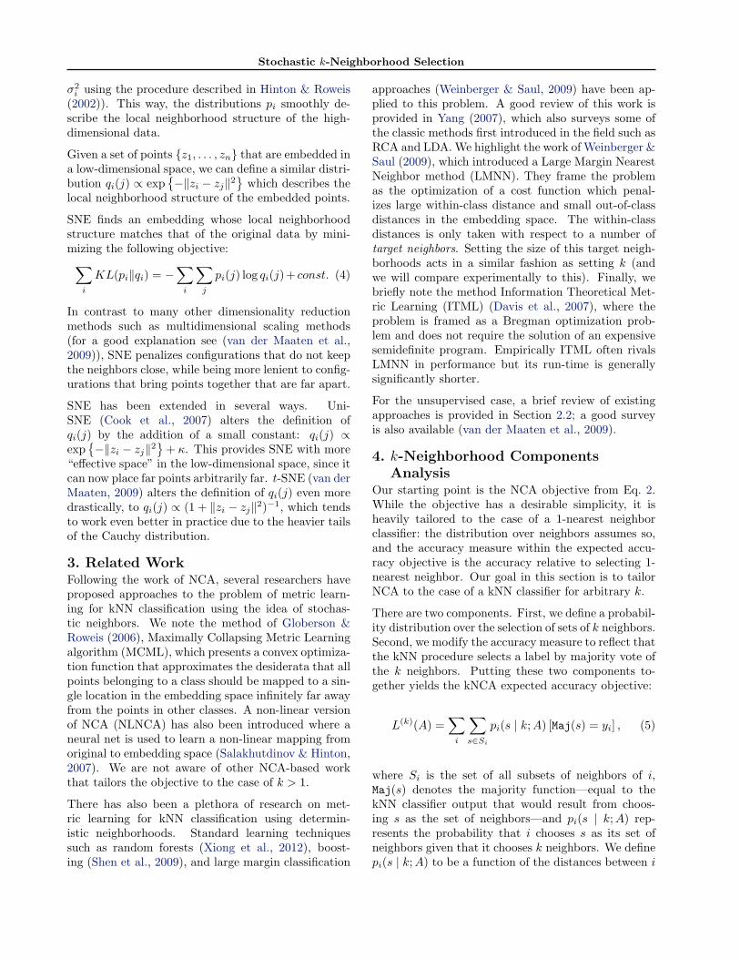
σ2i using the procedure described in Hinton & Roweis

(2002)). This way, the distributions pi smoothly de-scribe the local neighborhood structure of the high-dimensional data.

Given a set of points {z1, . . . , zn} that are embedded ina low-dimensional space, we can define a similar distri-bution qi(j) ∝ exp

{−‖zi − zj‖2

}which describes the

local neighborhood structure of the embedded points.

SNE finds an embedding whose local neighborhoodstructure matches that of the original data by mini-mizing the following objective:∑

i

KL(pi‖qi) = −∑

i

∑j

pi(j) log qi(j) + const. (4)

In contrast to many other dimensionality reductionmethods such as multidimensional scaling methods(for a good explanation see (van der Maaten et al.,2009)), SNE penalizes configurations that do not keepthe neighbors close, while being more lenient to config-urations that bring points together that are far apart.

SNE has been extended in several ways. Uni-SNE (Cook et al., 2007) alters the definition ofqi(j) by the addition of a small constant: qi(j) ∝exp

{−‖zi − zj‖2

}+ κ. This provides SNE with more

“effective space” in the low-dimensional space, since itcan now place far points arbitrarily far. t-SNE (van derMaaten, 2009) alters the definition of qi(j) even moredrastically, to qi(j) ∝ (1 + ‖zi − zj‖2)−1, which tendsto work even better in practice due to the heavier tailsof the Cauchy distribution.

3. Related WorkFollowing the work of NCA, several researchers haveproposed approaches to the problem of metric learn-ing for kNN classification using the idea of stochas-tic neighbors. We note the method of Globerson &Roweis (2006), Maximally Collapsing Metric Learningalgorithm (MCML), which presents a convex optimiza-tion function that approximates the desiderata that allpoints belonging to a class should be mapped to a sin-gle location in the embedding space infinitely far awayfrom the points in other classes. A non-linear versionof NCA (NLNCA) has also been introduced where aneural net is used to learn a non-linear mapping fromoriginal to embedding space (Salakhutdinov & Hinton,2007). We are not aware of other NCA-based workthat tailors the objective to the case of k > 1.

There has also been a plethora of research on met-ric learning for kNN classification using determin-istic neighborhoods. Standard learning techniquessuch as random forests (Xiong et al., 2012), boost-ing (Shen et al., 2009), and large margin classification

approaches (Weinberger & Saul, 2009) have been ap-plied to this problem. A good review of this work isprovided in Yang (2007), which also surveys some ofthe classic methods first introduced in the field such asRCA and LDA. We highlight the work of Weinberger &Saul (2009), which introduced a Large Margin NearestNeighbor method (LMNN). They frame the problemas the optimization of a cost function which penal-izes large within-class distance and small out-of-classdistances in the embedding space. The within-classdistances is only taken with respect to a number oftarget neighbors. Setting the size of this target neigh-borhoods acts in a similar fashion as setting k (andwe will compare experimentally to this). Finally, webriefly note the method Information Theoretical Met-ric Learning (ITML) (Davis et al., 2007), where theproblem is framed as a Bregman optimization prob-lem and does not require the solution of an expensivesemidefinite program. Empirically ITML often rivalsLMNN in performance but its run-time is generallysignificantly shorter.

For the unsupervised case, a brief review of existingapproaches is provided in Section 2.2; a good surveyis also available (van der Maaten et al., 2009).

4. k-Neighborhood ComponentsAnalysis

Our starting point is the NCA objective from Eq. 2.While the objective has a desirable simplicity, it isheavily tailored to the case of a 1-nearest neighborclassifier: the distribution over neighbors assumes so,and the accuracy measure within the expected accu-racy objective is the accuracy relative to selecting 1-nearest neighbor. Our goal in this section is to tailorNCA to the case of a kNN classifier for arbitrary k.

There are two components. First, we define a probabil-ity distribution over the selection of sets of k neighbors.Second, we modify the accuracy measure to reflect thatthe kNN procedure selects a label by majority vote ofthe k neighbors. Putting these two components to-gether yields the kNCA expected accuracy objective:

L(k)(A) =∑

i

∑s∈Si

pi(s | k;A) [Maj(s) = yi] , (5)

where Si is the set of all subsets of neighbors of i,Maj(s) denotes the majority function—equal to thekNN classifier output that would result from choos-ing s as the set of neighbors—and pi(s | k;A) rep-resents the probability that i chooses s as its set ofneighbors given that it chooses k neighbors. We definepi(s | k;A) to be a function of the distances between i


k = 1 k > 1

Figure 1. An illustration of the effect of k on the kNCA ob-jective. (left) When k = 1, two points can be isolated fromothers in their class and have no pressure to seek out largerclusters. (right) When k is greater than 1, small clusters ofpoints have greater pressure to join larger clusters, leadingthe objective to favor larger consistent groups of points.

and the points j ∈ s as follows:

pi(s | k;A) ={ 1

Z(A) exp{−∑

j∈s dij(A)} if |s| = k

0 otherwise,

where we use the shorthand dij = dij(A) = ||Axi −Axj ||22. While it is not yet obvious that Eq. 5 can beoptimized efficiently, as the normalization Z = Z(A)entails considering all subsets of size k, it should beclear that it is the expected accuracy of a kNN clas-sifier in the same way that the NCA objective is theexpected accuracy of a 1NN classifier. Indeed, withk = 1 we recover NCA.

5. Efficient Computation

The main computational observation in this work isthat Eq. 5 can be computed and optimized efficiently.To describe how, we begin by rewriting the inner sum-mation from Eq. 5 (throughout this section, we willfocus on the objective for a single point i, and willdrop dependencies on i in the notation):∑

s:|s|=k exp{−∑

j∈s dij} [Maj(s) = yi]∑s∈S:|s|=k exp{−

∑j∈s dij}

, (6)

Our strategy is to formulate a set of factor graphs torepresent the components of this problem such that theobjective can be expressed as a sum of ratios of parti-tion functions. Afterwards, we will show how efficientexact inference can be done on these factor graphs.

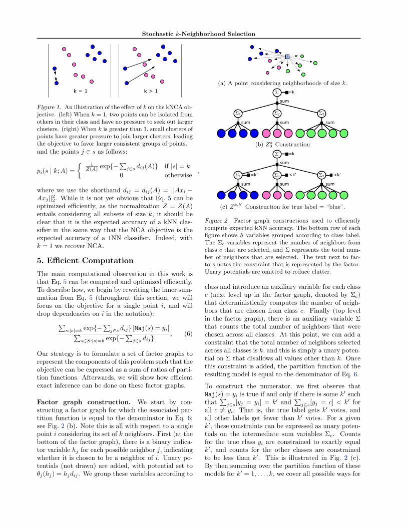
Factor graph construction. We start by con-structing a factor graph for which the associated par-tition function is equal to the denominator in Eq. 6;see Fig. 2 (b). Note this is all with respect to a singlepoint i considering its set of k neighbors. First (at thebottom of the factor graph), there is a binary indica-tor variable hj for each possible neighbor j, indicatingwhether it is chosen to be a neighbor of i. Unary po-tentials (not drawn) are added, with potential set toθj(hj) = hjdij . We group these variables according to

?

(a) A point considering neighborhoods of size k.

sum sum sum

=k

sum

!1 !2 !3

!

(b) Zk0 Construction

<k'<k'=k'

sum sum sum

=k

sum

!1 !2 !3

!

(c) Zk,k′

1 Construction for true label = “blue”.

Figure 2. Factor graph constructions used to efficientlycompute expected kNN accuracy. The bottom row of eachfigure shows h variables grouped according to class label.The Σc variables represent the number of neighbors fromclass c that are selected, and Σ represents the total num-ber of neighbors that are selected. The text next to fac-tors notes the constraint that is represented by the factor.Unary potentials are omitted to reduce clutter.

class and introduce an auxiliary variable for each classc (next level up in the factor graph, denoted by Σc)that deterministically computes the number of neigh-bors that are chosen from class c. Finally (top levelin the factor graph), there is an auxiliary variable Σthat counts the total number of neighbors that werechosen across all classes. At this point, we can add aconstraint that the total number of neighbors selectedacross all classes is k, and this is simply a unary poten-tial on Σ that disallows all values other than k. Oncethis constraint is added, the partition function of theresulting model is equal to the denominator of Eq. 6.

To construct the numerator, we first observe thatMaj(s) = yi is true if and only if there is some k′ suchthat

∑j∈s[yj = yi] = k′ and

∑j∈s[yj = c] < k′ for

all c 6= yi. That is, the true label gets k′ votes, andall other labels get fewer than k′ votes. For a givenk′, these constraints can be expressed as unary poten-tials on the intermediate sum variables Σc. Countsfor the true class yi are constrained to exactly equalk′, and counts for the other classes are constrainedto be less than k′. This is illustrated in Fig. 2 (c).By then summing over the partition function of thesemodels for k′ = 1, . . . , k, we cover all possible ways for


Maj(s) = yi to be true, and thus recover the numer-ator of Eq. 6. Specifically, Eq. 6 can be rewritten asfollows:

=

∑kk′=1

∑s:|s|=k exp{−

∑j∈s dij}[φk′(s)]∑

s∈S:|s|=k exp{−∑

j∈s dij}(7)

=∑k

k′=1 Zk,k′

1

Zk0

, where (8)

φk′(s)=(∑j∈s

[yj =yi]=k′) ∧ (∀c 6=yi,∑j∈s

[yj = c]<k′).

Efficient inference. At this point, we have reducedthe difficulty of the kNCA objective to computationof partition functions in the models constructed inthe previous section. If these partition functions canbe efficiently computed and differentiated, then thekNCA objective can be optimized.

The key observation is that the models in Fig. 2(b) and (c) are special cases of Recursive Cardinal-ity (RC) models (Tarlow et al., 2012). An RC modeldefines a probability distribution over binary vectorsh = (h1, . . . , hN ) based on an energy function of theform E(h) =

∑i θi(hi) +

∑s∈S fs(

∑j∈s hj), where S

is a set of subsets of {1, . . . , N} that must obey a nest-edness constraint: for all s, s′ ∈ S, either s ∩ s′ = ∅ ors ⊂ s′ or s′ ⊂ s. The fs(·) functions are arbitrary func-tions of the number of variables within the associatedsubset that take on value 1 and can be different foreach s. Given this energy function, an RC model de-fines the probability of a binary vector h as a standardGibbs distribution: p(h) = 1

Z exp{−E(h)}, where Zis the partition function that ensures the distributionsums to 1. The key utility of RC models is that thepartition function (and marginal distributions over allhi variables) can be computed efficiently. Briefly, in-ference works by constructing a binary tree that hashi variables at the leaves, and variables representingcounts of progressively larger subsets at internal nodes,then doing fast sum-product updates up and down thetree. See Tarlow et al. (2012) for more details.

For all applications of RC models considered here, thiscomputation of each partition function and associatedmarginals would take O(N log2N) time. Below, wealternatively show how to implement the same com-putations in O(Nk+Ck2) time (where recall N is thetotal number of points considered as neighbors, k is thenumber of neighbors to select, and C is the number ofclasses). For our purposes where k is typically small,and due to the smaller constant factors, an efficientC++ implementation of this algorithm outperformeda generic implementation from (Tarlow et al., 2012),so we used the special-purpose algorithm throughout.

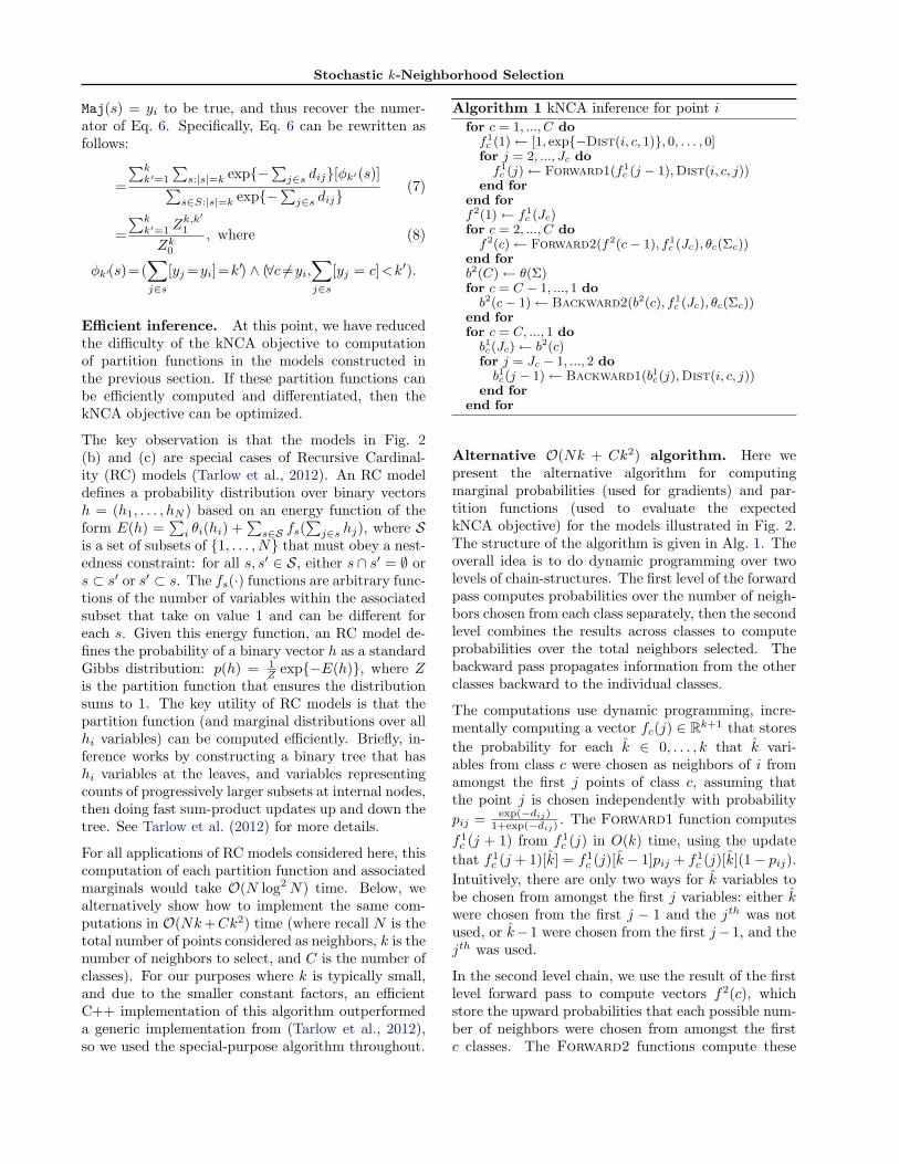
Algorithm 1 kNCA inference for point ifor c = 1, ..., C dof1

c (1)← [1, exp{−Dist(i, c, 1)}, 0, . . . , 0]for j = 2, ..., Jc dof1

c (j)← Forward1(f1c (j − 1),Dist(i, c, j))

end forend forf2(1)← f1

c (Jc)for c = 2, ..., C dof2(c)← Forward2(f2(c− 1), f1

c (Jc), θc(Σc))end forb2(C)← θ(Σ)for c = C − 1, ..., 1 dob2(c− 1)← Backward2(b2(c), f1

c (Jc), θc(Σc))end forfor c = C, ..., 1 dob1c(Jc)← b2(c)for j = Jc − 1, ..., 2 dob1c(j − 1)← Backward1(b1c(j),Dist(i, c, j))

end forend for

Alternative O(Nk + Ck2) algorithm. Here wepresent the alternative algorithm for computingmarginal probabilities (used for gradients) and par-tition functions (used to evaluate the expectedkNCA objective) for the models illustrated in Fig. 2.The structure of the algorithm is given in Alg. 1. Theoverall idea is to do dynamic programming over twolevels of chain-structures. The first level of the forwardpass computes probabilities over the number of neigh-bors chosen from each class separately, then the secondlevel combines the results across classes to computeprobabilities over the total neighbors selected. Thebackward pass propagates information from the otherclasses backward to the individual classes.

The computations use dynamic programming, incre-mentally computing a vector fc(j) ∈ Rk+1 that storesthe probability for each k̂ ∈ 0, . . . , k that k̂ vari-ables from class c were chosen as neighbors of i fromamongst the first j points of class c, assuming thatthe point j is chosen independently with probabilitypij = exp(−dij)

1+exp(−dij). The Forward1 function computes

f1c (j + 1) from f1

c (j) in O(k) time, using the updatethat f1

c (j + 1)[k̂] = f1c (j)[k̂ − 1]pij + f1

c (j)[k̂](1− pij).Intuitively, there are only two ways for k̂ variables tobe chosen from amongst the first j variables: either k̂were chosen from the first j − 1 and the jth was notused, or k̂−1 were chosen from the first j−1, and thejth was used.

In the second level chain, we use the result of the firstlevel forward pass to compute vectors f2(c), whichstore the upward probabilities that each possible num-ber of neighbors were chosen from amongst the firstc classes. The Forward2 functions compute these


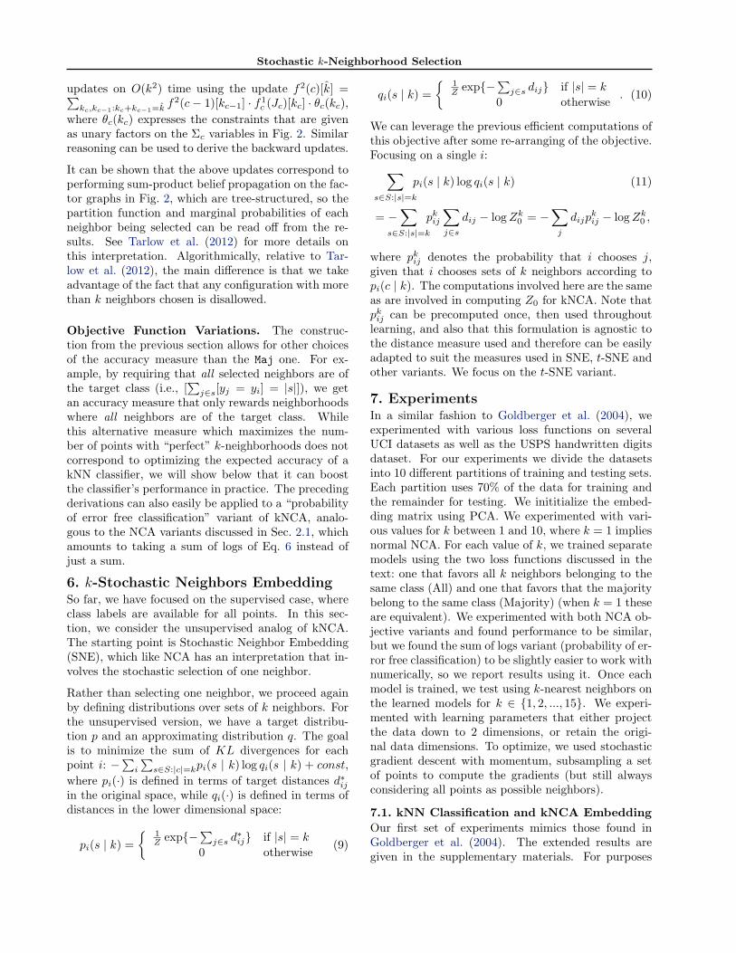
updates on O(k2) time using the update f2(c)[k̂] =∑kc,kc−1:kc+kc−1=k̂ f

2(c− 1)[kc−1] · f1c (Jc)[kc] · θc(kc),

where θc(kc) expresses the constraints that are givenas unary factors on the Σc variables in Fig. 2. Similarreasoning can be used to derive the backward updates.

It can be shown that the above updates correspond toperforming sum-product belief propagation on the fac-tor graphs in Fig. 2, which are tree-structured, so thepartition function and marginal probabilities of eachneighbor being selected can be read off from the re-sults. See Tarlow et al. (2012) for more details onthis interpretation. Algorithmically, relative to Tar-low et al. (2012), the main difference is that we takeadvantage of the fact that any configuration with morethan k neighbors chosen is disallowed.

Objective Function Variations. The construc-tion from the previous section allows for other choicesof the accuracy measure than the Maj one. For ex-ample, by requiring that all selected neighbors are ofthe target class (i.e., [

∑j∈s[yj = yi] = |s|]), we get

an accuracy measure that only rewards neighborhoodswhere all neighbors are of the target class. Whilethis alternative measure which maximizes the num-ber of points with “perfect” k-neighborhoods does notcorrespond to optimizing the expected accuracy of akNN classifier, we will show below that it can boostthe classifier’s performance in practice. The precedingderivations can also easily be applied to a “probabilityof error free classification” variant of kNCA, analo-gous to the NCA variants discussed in Sec. 2.1, whichamounts to taking a sum of logs of Eq. 6 instead ofjust a sum.

6. k-Stochastic Neighbors EmbeddingSo far, we have focused on the supervised case, whereclass labels are available for all points. In this sec-tion, we consider the unsupervised analog of kNCA.The starting point is Stochastic Neighbor Embedding(SNE), which like NCA has an interpretation that in-volves the stochastic selection of one neighbor.

Rather than selecting one neighbor, we proceed againby defining distributions over sets of k neighbors. Forthe unsupervised version, we have a target distribu-tion p and an approximating distribution q. The goalis to minimize the sum of KL divergences for eachpoint i: −

∑i

∑s∈S:|c|=kpi(s | k) log qi(s | k) + const,

where pi(·) is defined in terms of target distances d∗ijin the original space, while qi(·) is defined in terms ofdistances in the lower dimensional space:

pi(s | k) ={

1Z exp{−

∑j∈s d

∗ij} if |s| = k

0 otherwise(9)

qi(s | k) ={

1Z exp{−

∑j∈s dij} if |s| = k

0 otherwise. (10)

We can leverage the previous efficient computations ofthis objective after some re-arranging of the objective.Focusing on a single i:∑s∈S:|s|=k

pi(s | k) log qi(s | k) (11)

= −∑

s∈S:|s|=k

pkij

∑j∈s

dij − logZk0 = −

∑j

dijpkij − logZk

0 ,

where pkij denotes the probability that i chooses j,

given that i chooses sets of k neighbors according topi(c | k). The computations involved here are the sameas are involved in computing Z0 for kNCA. Note thatpk

ij can be precomputed once, then used throughoutlearning, and also that this formulation is agnostic tothe distance measure used and therefore can be easilyadapted to suit the measures used in SNE, t-SNE andother variants. We focus on the t-SNE variant.

7. ExperimentsIn a similar fashion to Goldberger et al. (2004), weexperimented with various loss functions on severalUCI datasets as well as the USPS handwritten digitsdataset. For our experiments we divide the datasetsinto 10 different partitions of training and testing sets.Each partition uses 70% of the data for training andthe remainder for testing. We inititialize the embed-ding matrix using PCA. We experimented with vari-ous values for k between 1 and 10, where k = 1 impliesnormal NCA. For each value of k, we trained separatemodels using the two loss functions discussed in thetext: one that favors all k neighbors belonging to thesame class (All) and one that favors that the majoritybelong to the same class (Majority) (when k = 1 theseare equivalent). We experimented with both NCA ob-jective variants and found performance to be similar,but we found the sum of logs variant (probability of er-ror free classification) to be slightly easier to work withnumerically, so we report results using it. Once eachmodel is trained, we test using k-nearest neighbors onthe learned models for k ∈ {1, 2, ..., 15}. We experi-mented with learning parameters that either projectthe data down to 2 dimensions, or retain the origi-nal data dimensions. To optimize, we used stochasticgradient descent with momentum, subsampling a setof points to compute the gradients (but still alwaysconsidering all points as possible neighbors).

7.1. kNN Classification and kNCA EmbeddingOur first set of experiments mimics those found inGoldberger et al. (2004). The extended results aregiven in the supplementary materials. For purposes


1-NCA (train) 5-NCA (train) 10-NCA (train)

1-NCA (test) 5-NCA (test) 10-NCA (test)

(a) Embeddings for Majority

1-NCA (train) 5-NCA (train) 10-NCA (train)

1-NCA (test) 5-NCA (test) 10-NCA (test)

(b) Embeddings for All

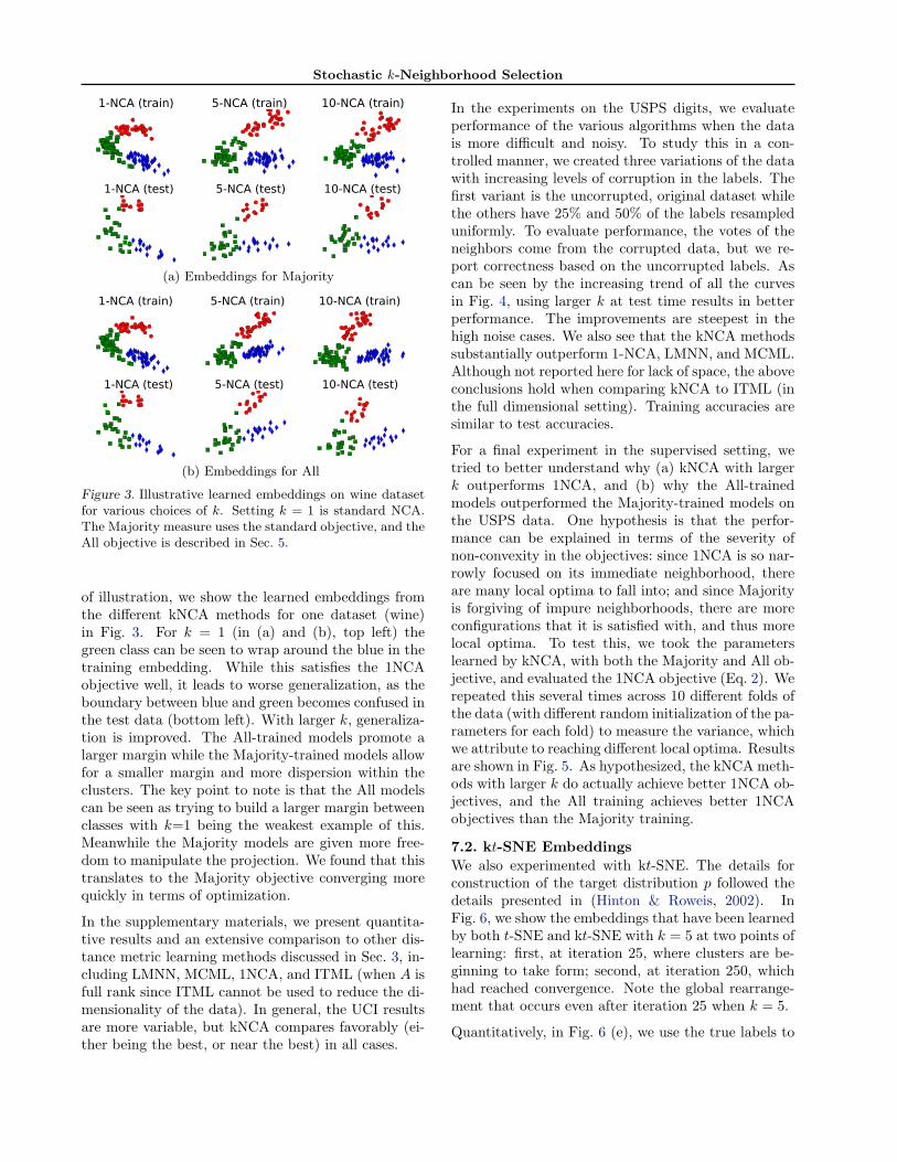
Figure 3. Illustrative learned embeddings on wine datasetfor various choices of k. Setting k = 1 is standard NCA.The Majority measure uses the standard objective, and theAll objective is described in Sec. 5.

of illustration, we show the learned embeddings fromthe different kNCA methods for one dataset (wine)in Fig. 3. For k = 1 (in (a) and (b), top left) thegreen class can be seen to wrap around the blue in thetraining embedding. While this satisfies the 1NCAobjective well, it leads to worse generalization, as theboundary between blue and green becomes confused inthe test data (bottom left). With larger k, generaliza-tion is improved. The All-trained models promote alarger margin while the Majority-trained models allowfor a smaller margin and more dispersion within theclusters. The key point to note is that the All modelscan be seen as trying to build a larger margin betweenclasses with k=1 being the weakest example of this.Meanwhile the Majority models are given more free-dom to manipulate the projection. We found that thistranslates to the Majority objective converging morequickly in terms of optimization.

In the supplementary materials, we present quantita-tive results and an extensive comparison to other dis-tance metric learning methods discussed in Sec. 3, in-cluding LMNN, MCML, 1NCA, and ITML (when A isfull rank since ITML cannot be used to reduce the di-mensionality of the data). In general, the UCI resultsare more variable, but kNCA compares favorably (ei-ther being the best, or near the best) in all cases.

In the experiments on the USPS digits, we evaluateperformance of the various algorithms when the datais more difficult and noisy. To study this in a con-trolled manner, we created three variations of the datawith increasing levels of corruption in the labels. Thefirst variant is the uncorrupted, original dataset whilethe others have 25% and 50% of the labels resampleduniformly. To evaluate performance, the votes of theneighbors come from the corrupted data, but we re-port correctness based on the uncorrupted labels. Ascan be seen by the increasing trend of all the curvesin Fig. 4, using larger k at test time results in betterperformance. The improvements are steepest in thehigh noise cases. We also see that the kNCA methodssubstantially outperform 1-NCA, LMNN, and MCML.Although not reported here for lack of space, the aboveconclusions hold when comparing kNCA to ITML (inthe full dimensional setting). Training accuracies aresimilar to test accuracies.

For a final experiment in the supervised setting, wetried to better understand why (a) kNCA with largerk outperforms 1NCA, and (b) why the All-trainedmodels outperformed the Majority-trained models onthe USPS data. One hypothesis is that the perfor-mance can be explained in terms of the severity ofnon-convexity in the objectives: since 1NCA is so nar-rowly focused on its immediate neighborhood, thereare many local optima to fall into; and since Majorityis forgiving of impure neighborhoods, there are moreconfigurations that it is satisfied with, and thus morelocal optima. To test this, we took the parameterslearned by kNCA, with both the Majority and All ob-jective, and evaluated the 1NCA objective (Eq. 2). Werepeated this several times across 10 different folds ofthe data (with different random initialization of the pa-rameters for each fold) to measure the variance, whichwe attribute to reaching different local optima. Resultsare shown in Fig. 5. As hypothesized, the kNCA meth-ods with larger k do actually achieve better 1NCA ob-jectives, and the All training achieves better 1NCAobjectives than the Majority training.

7.2. kt-SNE EmbeddingsWe also experimented with kt-SNE. The details forconstruction of the target distribution p followed thedetails presented in (Hinton & Roweis, 2002). InFig. 6, we show the embeddings that have been learnedby both t-SNE and kt-SNE with k = 5 at two points oflearning: first, at iteration 25, where clusters are be-ginning to take form; second, at iteration 250, whichhad reached convergence. Note the global rearrange-ment that occurs even after iteration 25 when k = 5.

Quantitatively, in Fig. 6 (e), we use the true labels to


1 3 5 7 9 11 13 15k used in evaluation

0.3

0.5

0.7

kNN

acc

ura

cy

1-NCA

3-NCA (Maj)

5-NCA (Maj)

10-NCA (Maj)

3-NCA (All)

5-NCA (All)

10-NCA (All)

LMNN (1)

LMNN (3)

LMNN (5)

LMNN (10)

MCML


0.3

0.5

0.7

kNN

acc

ura

cy

Test, 0 noise Test, 0.5 noise

Figure 4. Test accuracies on USPS digits data for projec-tions to 2 dimensions with varying levels of noise. 0.25noise is omitted for space but interpolated 0 and 0.5.

1 3 5 10k used at training time

0.34

0.36

0.38

0.40

0.42

0.44

0.46

0.48

NC

A o

bje

ctiv

e


0.16

0.17

0.18

0.19

0.20

0.21

0.22

NC

A o

bje

ctiv

e


0.120

0.125

0.130

0.135

0.140

NC

A o

bje

ctiv

e

0% noise 25% noise 50% noise

Figure 5. Mean and standard deviations of training 1-NCA objectives achieved by optimizing kNCA objectivesfor varying k (higher is better). Legend follows Fig. 4.

measure the leave-one-out accuracy for a kNN classi-fier applied to the points output by t-SNE and kt-SNE.t-SNE performs better on 1-nearest neighbor accuracy,but when k is increased, 5t-SNE overtakes t-SNE. Thisfurther illustrates the myopic nature of using k = 1in t-SNE. In the supplementary material, we provideanimations illustrating the evolution of kSNE embed-dings on USPS digits for various choices of k. In theseanimations, qualitative differences are visible, where t-SNE exhibits the myopic behavior illustrated in Fig. 1.

8. Discussion

There are several desirable properties of kNCA. First,it provides a proper methodology for doing NCA-likelearning when the desire is to use kNN with k > 1at test time. Our work here derives the NCA-like ob-jective that is properly matched to using kNN at testtime. kNN classifiers are ubiquitous, and a choice ofk > 1 is nearly always used, so the method has wideapplicability. Second, it provides robustness in twoways: first, the majority objective is relatively uncon-cerned with outliers, so long as the majority of neigh-bors in a region have the correct label; second, theobjective optimizes an expectation over the selectionof all sets of k neighbors, so we do not expect smallperturbations in the data to have a significant effecton the learning objective. Robustness is not achieved

(a) t-SNE iter 25 (b) t-SNE iter 250

(c) 5t-SNE iter 25 (d) 5t-SNE iter 250

k = 1 k = 5 k = 9 k = 13t-SNE 0.934 0.925 0.916 0.914

5t-SNE 0.928 0.946 0.953 0.949(e) kNN accuracy after unsupervised learning.

Figure 6. Unsupervised USPS digits results.

by the methods we compare to, which we attribute toeither their global or non-probabilistic nature.

Curiously, in most cases, the All objective outper-formed the Majority objective. The argument canbe made that All is like a margin-enhanced version ofMajority, which inherits robustness due to the prob-abilistic formulation, but generalizes well due to itsmargin-enforcing tendencies. We believe this to be aninteresting result for those people wishing to designbetter learning objectives; it challenges the commonintuition that the best learning objective is to mini-mize expected loss. However, our final supervised ex-periments suggest that the story may be more com-plicated, and that we might need to find better waysof initializing and optimizing the two methods beforehaving a clear answer.

One disadvantage of NCA (and thus also kNCA) isthe inherently quadratic nature of the algorithm thatcomes from basing it on pairwise distances. We be-lieve the method to still have desirable properties whenthe set of potential neighbors is restricted (either ran-domly or deterministically) but a fuller exploration ofthe tradeoffs involved require further investigation.

Finally, we believe the general technique used to com-pute the expected majority function to be of interestbeyond just for kNN classifiers and for kNCA learning.It would be interesting to find further applications.


References

Balasubramanian, M., Shwartz, E. L., Tenenbaum, J. B.,de Silva, V., and Langford, J. C. The isomap algorithmand topological stability. Science, 2002.

Cook, JA, Sutskever, I., Mnih, A., and Hinton, GE. Visual-izing similarity data with a mixture of maps. Proceedingsof the International Conference on Artificial Intelligenceand Statistics (AISTATS), 2007.

Davis, Jason V., Kulis, Brian, Jain, Prateek, Sra, Suvrit,and Dhillon, Inderjit S. Information-theoretic metriclearning. In Proceedings of the International Conferenceon Machine Learning (ICML), 2007.

Globerson, Amir and Roweis, Sam T. Metric learning bycollapsing classes. In Advances in Neural InformationProcessing Systems (NIPS), 2006.

Goldberger, Jacob, Roweis, Sam T., Hinton, Geoffrey E.,and Salakhutdinov, Ruslan. Neighbourhood componentsanalysis. In Advances in Neural Information ProcessingSystems (NIPS), 2004.

Hinton, Geoffrey E. and Roweis, Sam T. Stochastic neigh-bor embedding. In Advances in Neural Information Pro-cessing Systems (NIPS), 2002.

Roweis, Sam T. and Saul, Lawrence K. Nonlinear dimen-sionality reduction by locally linear embedding. Science,290, 2000.

Salakhutdinov, Ruslan and Hinton, Geoffrey. Learning anonlinear embedding by preserving class neighbourhoodstructure. In Proceedings of the International Conferenceon Artificial Intelligence and Statistics (AISTATS), vol-ume 11, 2007.

Shen, Chunhua, Kim, Junae, Wang, Lei, and van den Hen-gel, Anton. Positive semidefinite metric learning withboosting. In Advances in Neural Information ProcessingSystems (NIPS). 2009.

Tarlow, Daniel, Swersky, Kevin, Zemel, Richard S.,Adams, Ryan P., and Frey, Brendan J. Fast exact infer-ence for recursive cardinality models. In Uncertainty inArtificial Intelligence (UAI), 2012.

van der Maaten, Laurens. Learning a parametric embed-ding by preserving local structure. In Proceedings of theInternational Conference on Artificial Intelligence andStatistics (AISTATS), 2009.

van der Maaten, L.J.P., Postma, E.O., and van den Herik,H.J. Dimensionality reduction: A comparative review.Technical Report TiCC-TR 2009-005, Tilburg Univer-sity, 2009.

Weinberger, K.Q. and Saul, L.K. Distance metric learningfor large margin nearest neighbor classification. Journalof Machine Learning Research (JMLR), 2009.

Xiong, Caiming, Johnson, David, Xu, Ran, and Corso,Jason J. Random forests for metric learning with im-plicit pairwise position dependence. In Proceedings of theInternational Conference on Knowledge Discovery andData Mining (SIGKDD), New York, NY, USA, 2012.ACM.

Yang, Liu. Distance metric learning: A comprehensivesurvey. Technical report, Carnegie Mellon University,2007.


Supplementary Materials for“Stochastic k-Neighborhood Selectionfor Supervised and UnsupervisedLearning”

Daniel Tarlow, Kevin Swersky, Laurent Char-lin, Ilya Sutskever, and Richard S. Zemel

On the following pages we provide the full quantitativeresults comparing kNCA to NCA, LMNN, MCML, and(when applicable) ITML on 7 datasets (4 UCI, plus USPSwith 3 noise levels).


0 2 4 6 8 10 12 14 16k used in evaluation

0.85

0.90

0.95

1.00

kNN

acc

ura

cy


0.78

0.81

0.84

0.87

0.90

kNN

acc

ura

cy0 2 4 6 8 10 12 14 16

k used in evaluation

0.85

0.90

0.95

1.00

kNN

acc

ura

cy


0.800

0.825

0.850

0.875

0.900

kNN

acc

ura

cy

Ion Train (dim 2) Ion Test (dim 2) Ion Train (dim full) Ion Test (dim full)


0.976

0.984

0.992

1.000

kNN

acc

ura

cy


0.94

0.96

0.98

kNN

acc

ura

cy


0.92

0.94

0.96

0.98

1.00

kNN

acc

ura

cy0 2 4 6 8 10 12 14 16

k used in evaluation

0.925

0.950

0.975

kNN

acc

ura

cy

Wine Train (dim 2) Wine Test (dim 2) Wine Train (dim full) Wine Test (dim full)


0.86

0.88

0.90

0.92

kNN

acc

ura

cy


0.86

0.88

0.90

0.92

kNN

acc

ura

cy


0.80

0.88

0.96

kNN

acc

ura

cy


0.80

0.88

0.96

kNN

acc

ura

cy

Balance Train (dim 2) Balance Test (dim 2) Balance Train (dim full) Balance Test (dim full)


0.960

0.975

0.990

kNN

acc

ura

cy


0.945

0.960

0.975

0.990

kNN

acc

ura

cy


0.960

0.975

0.990

kNN

acc

ura

cy


0.945

0.960

0.975

0.990

kNN

acc

ura

cy

Iris Train (dim 2) Iris Test (dim 2) Iris Train (dim full) Iris Test (dim full)


0.3

0.5

0.7

kNN

acc

ura

cy


0.3

0.5

0.7

kNN

acc

ura

cy


0.91

0.92

0.93

0.94

0.95

0.96

0.97

0.98

0.99

kNN

acc

ura

cy

1-NCA

3-NCA (Maj)

5-NCA (Maj)

10-NCA (Maj)

3-NCA (All)

5-NCA (All)

10-NCA (All)

ITML

LMNN (1)

LMNN (3)

LMNN (5)

LMNN (10)

MCML


0.90

0.91

0.92

0.93

0.94

0.95

0.96

0.97

kNN

acc

ura

cy

USPS 0% noise Train (dim 2) USPS 0% noise Test (dim 2) USPS 0% noise Train (dim full) USPS 0% noise Test (dim full)



0.3

0.5

0.7

kNN

acc

ura

cy


0.3

0.5

0.7

kNN

acc

ura

cy


0.70

0.75

0.80

0.85

0.90

0.95

1.00

kNN

acc

ura

cy


0.70

0.75

0.80

0.85

0.90

0.95

kNN

acc

ura

cy



0.3

0.5

0.7

kNN

acc

ura

cy


0.3

0.5

0.7

kNN

acc

ura

cy


0.50

0.55

0.60

0.65

0.70

0.75

0.80

0.85

0.90

0.95

kNN

acc

ura

cy


0.50

0.55

0.60

0.65

0.70

0.75

0.80

0.85

0.90

0.95

kNN

acc

ura

cy

1-NCA

3-NCA (Maj)

5-NCA (Maj)

10-NCA (Maj)

3-NCA (All)

5-NCA (All)

10-NCA (All)

ITML

LMNN (1)

LMNN (3)

LMNN (5)

LMNN (10)

MCML


stochastic k-neighborhood selection for supervised and ...dtarlow/tarswercharsutzem_icml2013.pdf ·...

Documents