“usepackageamstex12beta.

Stochastic Modeling in Operations Research(incomplete classnotes)

version 1/17/2007

1

Contents

1 What is Operations Research ? 3

2 Review of Probability Theory and Random Variables 6

1 Probability Theory . . . . . . . . . . . . . . . . . . . . . . . . . . . . . . . . . . . 6

2 Discrete Random Variables . . . . . . . . . . . . . . . . . . . . . . . . . . . . . . 9

3 Continuous Random Variables . . . . . . . . . . . . . . . . . . . . . . . . . . . . . 10

4 Review of Probability Distributions . . . . . . . . . . . . . . . . . . . . . . . . . . 11

3 Markov Chains 16

1 Stochastic Processes . . . . . . . . . . . . . . . . . . . . . . . . . . . . . . . . . . 16

2 Markov Chains . . . . . . . . . . . . . . . . . . . . . . . . . . . . . . . . . . . . . 16

3 More M.C. Examples . . . . . . . . . . . . . . . . . . . . . . . . . . . . . . . . . . 25

4 Long-run Properties of M.C. . . . . . . . . . . . . . . . . . . . . . . . . . . . . . . 28

4.1 Gambler’s Ruin Problem (absorbing states) . . . . . . . . . . . . . . . . . 30

4.2 Sums of Independent, Identically Distributed, Random Variables . . . . . 37

4 Poisson and Markov Processes 42

1 The Poisson Process . . . . . . . . . . . . . . . . . . . . . . . . . . . . . . . . . . 42

2 Markov Process . . . . . . . . . . . . . . . . . . . . . . . . . . . . . . . . . . . . . 44

2.1 Rate Properties of Markov Processes . . . . . . . . . . . . . . . . . . . . . 45

5 Queueing Models I 48

1 Terminology . . . . . . . . . . . . . . . . . . . . . . . . . . . . . . . . . . . . . . . 48

2 The Birth-Death Process . . . . . . . . . . . . . . . . . . . . . . . . . . . . . . . . 50

3 Models Based on the B-D Process . . . . . . . . . . . . . . . . . . . . . . . . . . 52

4 M/M/1 Model . . . . . . . . . . . . . . . . . . . . . . . . . . . . . . . . . . . . . 52

5 M/M/c/∞/∞ . . . . . . . . . . . . . . . . . . . . . . . . . . . . . . . . . . . . . . 58

6 Finite Buffer Models) . . . . . . . . . . . . . . . . . . . . . . . . . . . . . . . . . 62

7 M/M/c/c Erlang Loss Model . . . . . . . . . . . . . . . . . . . . . . . . . . . . . 68

8 M/M/∞/∞ Unlimited Service Model . . . . . . . . . . . . . . . . . . . . . . . . 69

2

9 Finite Population Models . . . . . . . . . . . . . . . . . . . . . . . . . . . . . . . 70

10 System Availability . . . . . . . . . . . . . . . . . . . . . . . . . . . . . . . . . . . 74

11 Double Ended Queue . . . . . . . . . . . . . . . . . . . . . . . . . . . . . . . . . . 77

6 System Reliability 80

1 Introduction . . . . . . . . . . . . . . . . . . . . . . . . . . . . . . . . . . . . . . . 80

2 Types of Systems . . . . . . . . . . . . . . . . . . . . . . . . . . . . . . . . . . . . 81

3 System Reliability . . . . . . . . . . . . . . . . . . . . . . . . . . . . . . . . . . . 81

4 Reliability Using Failure Rates . . . . . . . . . . . . . . . . . . . . . . . . . . . . 83

7 Appedix 87

1 Final Project Guidelines . . . . . . . . . . . . . . . . . . . . . . . . . . . . . . . . 88

3

Chapter 1

What is Operations Research ?

Contents.

Definitions

Phases of an OR study

Principles of Modeling

Two definitions.

(1) O.R. is concerned with scientifically deciding how best to design and operate systems,

usually under conditions requiring the allocation of scarce resources.

(2) O.R. is a scientific approach to decision making.

Modern Definition. (suggested but not adopted yet)

Operations research (OR) is the application of scientific methods to improve the effectiveness

of operations, decisions and management. By means such as analyzing data, creating math-

ematical models and proposing innovative approaches, Or professionals develop scientifically

based information that gives insight and guides decision making. They also develop related

software, systems, services and products.

Clarification.

Or professionals collaborate with clients to design and improve operations, make better

decisions, solve problems and advance other managerial functions including policy formulation,

planning, forecasting and performance measurement. Clients may be executive, managerial or

non-managerial.

These professionals develop information to improve valuable insight and guidance. They

apply the most appropriate scientific techniques-selected from mathematics, any of the sciences

including social and management sciences, and any branch of engineering. their work normally

entails collecting and analyzing data, creating and testing mathematical models, proposing

approaches not previously considered, interpreting information, making recommendations, and

helping implement the initiatives that result.

Moreover, they develop and help implement software, systems, services and products related

to their methods and applications. The systems include strategic decisions-support systems,

4

which play vital role in many organizations. (Reference: Welcome to OR territory by Randy

Robinson, ORMS today,pp40-43.)

System. A collection of parts, making up a coherent whole.

Examples. Stoplights, city hospital, telephone switch board, etc.

Problems that are amenable to OR methodologies

(1) Water dams, business decisions like what product to introduce in the market, packaging

designs (Markov chains).

(2) Telephone systems, stoplights, communication systems, bank tellers (queueing theory).

(3) Inventory control: How much to stock?

(4) What stocks to buy? When to sell your house? When to perform preventive Mainte-

nance? (Markov decision processes)

(5) How reliable a system is? Examples: car, airplane, manufacturing process.

What is the probability that a system would not fail during a certain period of time?

How to pick a system design that improves reliability?

(6) Simulation

∗ Complex systems

∗ Example. How to generate random numbers using computers? How to simulate the

behavior of a complex communications system?

(7) Linear Programming: How is a long-distance call routed from its origin to its destination?

Phases of an O.R. study

(1) Formulating the problem: Parameters; decisions variables or unknowns; constraints;

objective function.

(2) Model construction: Building a mathematical model

(3) Performing the Analysis: (i) solution of the model (analytic, numerical,approximate,

simulation,...,etc.) (ii) sensitivity analysis.

(4) Model evaluation: Are the answers realistic?

(5) Implementation of teh findings and updating of the Model

Types of Models

(1) Deterministic (Linear programming, integer programming, network analysis,...,etc)

(2) Probabilistic (Queueing models, systems reliability, simulation, ...etc)

(3) Axiomatic: Pure mathematical fields (measure theory, set theory, probability theory, ...

etc)

The Modeling Process.

Real system

Model

Model conclusions

Real conclusions

5

Principles of Modeling.

(1) All models are approximate; however some are better than others (survival of the fittest).

(2) Do not build a complicated model when a simple one will suffice.

(3) Do not model a problem merely to fit the technique.

(4) The deduction stage must be conducted rigorously.

(5) Models should be validated before implementation.

(6) A model should never be taken too literally (models should not replace reality.

(7) A model cannot be any better than the information that goes into it (GIGO).

6

Chapter 2

Review of Probability Theory andRandom Variables

Contents.

Probability Theory

Discrete Distributions

Continuous Distributions

1 Probability Theory

Definitions

Random experiment: involves obtaining observations of some kind

Examples Toss of a coin, throw a die, polling, inspecting an assembly line, counting arrivals

at emergency room, etc.

Population: Set of all possible observations. Conceptually, a population could be generated

by repeating an experiment indefinitely.

Outcome of an experiment:

Elementary event (simple event): one possible outcome of an experiment

Event (Compound event): One or more possible outcomes of a random experiment

Sample space: the set of all sample points for an experiment is called a sample space; or set

of all possible outcomes for an experiment

Notation:

Sample space : Ω

Sample point: ω

Event: A, B, C, D, E etc. (any capital letter).

Example. Ω = wi, i = 1, · · ·6, where wi = i. That is Ω = 1, 2, 3, 4, 5, 6. We may think of

Ω as representation of possible outcomes of a throw of a die.

More definitions

7

Union, Intersection and Complementation

Mutually exclusive (disjoint) events

Probability of an event:

Consider a random experiment whose sample space is Ω. For each event E of the sample

space Ω define a number P (E) that satisfies the following three axioms (conditions):

(i) 0 ≤ P (E) ≤ 1

(ii) P (Ω) = 1

(iii) For any sequence of mutually exclusive (disjoint) events E1, E2, . . .,

P (∪∞i=1Ei) =

∞∑

i=1

P (Ei).

We refer to P (E) as the probability of the event E.

Examples. Let Ω = E1, . . . , E10. It is known that P (Ei) = 1/20, i = 1, . . . , 5 and P (Ei) =

1/5, i = 7, . . . , 9 and P (E10) = 3/20.

Q1: Do these probabilities satisfy the axioms?

A: Yes

Q2: Calculate P (A) where A = Ei, i ≥ 6.A: P (A) = P (E6)+P (E7)+P (E8)+P (E9)+P (E10) = 1/20+1/5+1/5+1/5+3/20 = 0.75

Interpretations of Probability

(i) Relative frequency interpretation: If an experiment in repeated a large number, n, of

times and the event E is observed nE times, the probability of E is

P (E) ≃ nE

n

By the SLLN , P (E) = limn→∞nE

n .

(ii) In real world applications one observes (measures) relative frequencies, one cannot mea-

sure probabilities. However, one can estimate probabilities.

(iii) At the conceptual level we assign probabilities to events. The assignment, however,

should make sense. (e.g. P (H) = .5, p(T ) = .5 in a toss of a fair coin).

(iv) In some cases probabilities can be a measure of belief (subjective probability). This

measure of belief should however satisfy the axioms.

(v) Typically, we would like to assign probabilities to simple events directly; then use the

laws of probability to calculate the probabilities of compound events.

Laws of Probability

(i) Complementation law

P (Ec) = 1 − P (E)

(ii) Additive law

P (E ∪ F ) = P (E) + P (F ) − P (E ∩ F )

8

Moreover, if E and F are mutually exclusive

P (E ∪ F ) = P (E) + P (F )

Conditional Probability

Definition If P (B) > 0, then

P (A|B) =P (A ∩ B)

P (B)

(iii) Multiplicative law (Product rule)

P (A ∩ B) = P (A|B)P (B)

Definition. Any collection of events that is mutually exclusive and collectively exhaustive is

said to be a partition of the sample space Ω.

(iv) Law of total probability

Let the events A1, A2, . . . , An be a partition of the sample space Ω and let B denote an

arbitrary event. Then

P (B) =

n∑

i=1

P (B|Ai)P (Ai).

Theorem 1.1 (Bayes’ Theorem) Let the events A1, A2, . . . , An be a partition of the sample

space Ω and let B denote an arbitrary event, P (B) > 0. Then

P (Ak|B) =P (B|Ak)P (Ak)

∑ni=1 P (B|Ai)P (Ai)

.

Special case. Let the events A, Ac be a partition of the sample space Ω and let B denote an

arbitrary event, P (B) > 0. Then

P (A|B) =P (B|A)P (A)

P (B|A)P (A) + P (B|Ac)P (Ac).

Remarks.

(i) The events of interest here are Ak, P (Ak) are called prior probabilities, and P (Ak|B)

are called posterior probabilities.

(ii) Bayes’ Theorem is important in several fields of applications.

Independence

(i) Two events A and B are said to be independent if

P (A ∩ B) = P (A)P (B).

(ii) Two events A and B that are not independent are said to be dependent.

9

Random Sampling

Definition. A sample of size n is said to be a random sample if the n elements are selected

in such a way that every possible combination of n elements has an equal probability of being

selected.

In this case the sampling process is called simple random sampling.

Remarks. (i) If n is large, we say the random sample provides an honest representation of the

population.

(i) Tables of random numbers may be used to select random samples.

2 Discrete Random Variables

A random variable (r.v.) X is a real valued function defined on a sample space Ω. That

is a random variable is a rule that assigns probabilities to each possible outcome of a random

experiment.

Probability mass function (pmf)

For a discrete r.v., X , the function f(x) defined by f(x) = P (X = x) for each possible x is

said to be a Probability mass function (pmf)

Probability distribution function (cdf)

The cdf , F (x), of a discrete r.v., X , is the real valued function defined by the equation

F (x) = P (X ≤ x).

Proposition 2.1 Let X be a discrete r.v. with pmf f(x). Then

(i) 0 ≤ f(x) ≤ 1, and

(ii)∑

x f(x) = 1

where the summation is over all possible values of x.

Relations between pmf and cdf

(i) F (x) =∑

y≤x f(y) for all x

(ii)f(x) = F (x) − F (x−) for all x .

(iii)

P (a < X ≤ b) = F (b) − F (a).

Properties of Distribution Functions

(i) F is a non-decreasing function; that is if a < b, then F (a) ≤ F (b).

(ii) F (∞) = 1 and F (−∞) = 0.

(iii) F is right-continuous.

Expected Value and Variance

10

E[X ] =∑

x

xP (X = x)

=∑

x

xf(x).

E[g(X)] =∑

x

g(x)f(x)

µk = E[Xk] =∑

x

xkf(x), k = 1, 2, . . . .

Variance.

V (X) = E[(X − µ)2] =∑

x

(x− µ)2f(x)

A short cut for the variance is

V (X) = E[X2] − (E[X ])2

Notation: Sometimes we use σ2 = V (X).

σX =√

V (X) =√

E[(X − µ)2] =

√

∑

x

(x − µ)2f(x)

3 Continuous Random Variables

Probability distribution function (cdf)

A random variable X is said to be continuous if its cdf is a continuous function such that

FX(x) = P (X ≤ x) =

∫ x

−∞

fX(t)dt ;

fX(t) ≥ 0 ;∫ ∞

−∞

fX(t)dt = 1 .

For a continuous r.v., X , the function fX(x) is said to be a probability density function (pdf)

Proposition 3.1 Let X be a continuous r.v. with pdf f(x). Then

(i) 0 ≤ f(x) ≤ 1, and

(ii)∫

x f(x)dx = 1

where the integral is over the range of possible values of x.

11

Useful Relationships

(i)

P (a ≤ X ≤ b) = F (b) − F (a).

(ii)P (X = x) = F (x) − F (x−) = 0 for all x .

(iii) f(x) = F ′(x) for all x at which f is continuous.

Properties of Distribution Function

(i) F is a non-decreasing function; that is if a < b, then F (a) ≤ F (b).

(ii) F (∞) = 1 and F (−∞) = 0.

(iii) F is continuous.

Expected Value and Variance

µ = E[X ] =

∫ +∞

−∞

xf(x)dx

E[g(X)] =

∫ +∞

−∞

g(x)f(x)dx

µk = E[Xk] =

∫ +∞

−∞

xkf(x)dx, k = 1, 2, . . . .

Variance.

V (X) = E[(X − µ)2] =

∫ +∞

−∞

(x − µ)2f(x)dx

Shortcut Formula

V (X) = E[X2] − E[X ]2 = E[X2] − µ2

σX =√

V (X) =√

E[(X − µ)2]

4 Review of Probability Distributions

Contents.

Poisson distribution

Geometric distribution

Exponential distribution

Poisson.

The Poisson pmf arises when counting the number of events that occur in an interval of

time when the events are occurring at a constant rate; examples include number of arrivals at

an emergency room, number of items demanded from an inventory; number of items in a batch

of a random size.

12

A rv X is said to have a Poisson pmf with parameter λ > 0 if

f(x) = e−λλx/x!, x = 0, 1, . . . .

Mean: E[X ] = λ

Variance: V (X) = λ, σX =√

λ

Example. Suppose the number of typographical errors on a single page of your book has a

Poisson distribution with parameter λ = 1/2. Calculate the probability that there is at least

one error on this page.

Solution. Letting X denote the number of errors on a single page, we have

P (X ≥ 1) = 1 − P (X = 0) = 1− e−0.5 ≃ 0.395

Geometric

The geometric distribution arises in situations where one has to wait until the first success.

For example, in a sequence of coin tosses (with p =P(head)), the number of trials, X , until the

first head is thrown is a geometric rv.

A random variable X is said to have a geometric pmf with parameter p, 0 < p < 1, if

P (X = n) = qn−1p (n = 1, 2, . . . ; p > 0, q = 1− p) .

Properties.

(i)∑∞

n=1 P (X = n) = p∑∞

n=1 qn−1 = p/(1 − q) = 1.

(ii) Mean: E[X ] = 1p

(iii) Second Moment: E[X2] = 2p2 − 1

p

(iv) Variance: V (X) = qp2

(v) CDF Complement: P (X ≥ k) = qk−1

(iv) Memoryless Property: P (X = n + k|X > n) = P (X = k); k=1,2,. . . .

Modified Geometric Distribution

For example, in a sequence of coin tosses (with p =P(head)), the number of tails, X , until

the first head is thrown is a geometric rv. A random variable X is said to have a geometric

pmf with parameter p, 0 < p < 1, if

P (X = n) = qnp (n = 0, 1, . . . ; p > 0, q = 1 − p) .

Properties.

(i)∑∞

n=0 P (X = n) = p∑∞

n=0 qn = p/(1 − q) = 1.

(ii) Mean. E[X ] = qp

(iii) Second Moment. E[X2] = qp2 + q2

p2

13

(iv) Variance. V (X) = qp2

(v) CDF Complement. P (X ≥ k) = qk

(iv) Memoryless Property. P (X = n + k|X > n) = P (X = k).

Exponential.

The exponential pdf often arises, in practice, as being the distribution of the amount of

time until some specific event occurs. Examples include time until a new car breaks down, time

until an arrival at emergency room, ... etc.

A rv X is said to have an exponential pdf with parameter λ > 0 if

f(x) = λe−λx , x ≥ 0

= 0 elsewhere

Example. Suppose that the length of a phone call in minutes is an exponential rv with

parameter λ = 1/10. If someone arrives immediately ahead of you at a public telephone booth,

find the probability that you will have to wait (i) more than 10 minutes, and (ii) between 10

and 20 minutes.

Solution Let X be the be the length of a phone call in minutes by the person ahead of you.

(i)

P (X > 10) = F (10) = e−λx = e−1 ≃ 0.368

(ii)

P (10 < X < 20) = F (10)− F (20) = e−1 − e−2 ≃ 0.233

Properties

(i) Mean: E[X ] = 1/λ

(ii) Variance: V (X) = 1/λ2, σ = 1/λ

(iii) CDF: F (x) = 1− e−λx.

(iv) Memoryless Property

Definition 4.1 A non-negative random variable is said to be memoryless if

P (X > h + t|X > t) = P (X > h) for all h, t ≥ 0.

Proposition 4.2 The exponential rv has the memoryless property

Proof. The memoryless property is equivalent to

P (X > h + t; X > t)

P (X > t)= P (X > h)

14

or

P (X > h + t) = P (X > h)P (X > t)

or

F (h + t) = F (h)F (t)

For the exponential distribution,

F (h + t) = e−λ(h+t) = e−λhe−λt = F (h)F (t) .

Converse The exponential distribution is the only continuous distribution with the memoryless

property.

Proof. Omitted.

(v) Hazard Rate

The hazard rate (sometimes called the failure rate) function is defined by

h(t) =f(t)

1 − F (t)

For the exponential distribution

h(t) =f(t)

1 − F (t)

=λe−λt

e−λt

= λ .

(vi) Transform of the Exponential Distribution

Let E[e−θX ] be the Laplace-Stieltjes transform of X , θ > 0. Then

E[e−θX ] :=

∫ ∞

0

e−θxdF (x)

=

∫ ∞

0e−θxf(x)dx

=λ

λ + θ

(vii) Increment Property of the Exponential Distribution

Definition 4.3 The function f is said to be o(h) (written f = o(h)) if

limh→0

f(h)

h= 0.

15

Examples

(i) f(x) = x is not o(h), since

limh→0

f(h)

h= lim

h→0

h

h= 1 6= 0

(ii) f(x) = x2 is o(h), since

limh→0

f(h)

h= lim

h→0

h2

h= 0

Recall:

ex = 1 + x +x2

2!+

x3

3!+ · · ·

FACT.

P (t < X < t + h|X > t) = λh + o(h)

Proof.

P (t < X < t + h|X > t) = P (X < t + h|X > t)

= 1 − P (X > t + h|X > t)

= 1 − e−λh

= 1 − (1 − λh +(λh)2

2!

−(λh)3

3!+ · · · )

= λh + o(h).

(viii) Minimum of exponential r.v.s

FACT. Let X1, . . .Xk be independent exp (αi) rvs. Let X = minX1, X2, . . . , Xk, and α =

α1 + . . . + αk. Then X has an exponential distribution with parameter α.

Proof.

P (X > t) = P (X1 > t, . . . , Xk > t)

= P (X1 > t) · · ·P (Xk > t)

= e−α1t · · ·e−αkt

= e−(α1+...αk)t

= e−αt.

16

Chapter 3

Markov Chains

Contents.

Stochastic Processes

Markov Chains

Long-run Properties of M.C.

1 Stochastic Processes

A stochastic process, Xt; t ∈ T, T an index set, is a collection (family) of random variables;

where T is an index set and for each t, X(t) is a random variable.

Let S be the state space of Xt; t ∈ T. Assume S is countable.

Interpretation. A stochastic process is a representation of a system that evolved over time.

Examples. Weekly inventory levels, demands.

∗ At this level of generality, stochastic processes are difficult to analyze.

Index set T

T = [0,∞) continuous timeor T = [0, 1, 2, 3, · · · ) discrete time

Remarks.

(i) We interpret t as time, and call X(t) the state of the process at time t.

(ii) If the index set T a countable set, we call X a discrete-time stochastic process.

(iii) If T is continuous, we call we call X a continuous-time stochastic process.

(iv) Any realization of X is called a sample path. (i.e. the number of customers waiting to

be served).

2 Markov Chains

Definition. A discrete-time stochastic process Xn, n = 0, 1, . . . with integer state space is

said to be a Markov chain (M.C.) if it satisfies the Markovian property, i.e.

17

P (Xn+1 = j|X0 = x0, . . . , Xn−1 = xn−1, Xn = i)

= P (Xn+1 = j|Xn = i)

for every choice of the non-negative integer n and the numbers x0, . . .xn−1, i, j in S = I .

Interpretation. Future is independent of the past, it only depends on the present.

Better statement Future depends on the Past only through the Present (indirectly).

Notation. pij(n) = P (Xn+1 = j|Xn = i) are called the one-step transition probabilities.

Definition. A Markov chain Xn, n = 0, 1, . . . is said to have stationary (time-homogeneous)

transition probabilities if

P (Xn+1 = j|Xn = i) = P (X1 = j|X0 = i) ≡ pij

for all n = 0, 1, . . ..

Remarks.

(i) A rv is characterized by its distribution.

(ii) A stochastic process is, typically, characterized by its finite dimensional distributions.

(iii) A M.C. is characterized by its initial distribution and its one-step transition matrix.

P =

p00 p01 p02 . . .

p10 p11 p12 . . ....

......

Note that all entries in P are non-negative, and all rows add up to 1.

(iv) Chapman-Kolmogorov (C-K) equations.

Let p(m)ij be the m-step transition probability, i.e.

p(m)ij = P (Xm = j|X0 = i)

Then the C-K equations are

p(m)ij =

∑

r

p(m−k)ir p

(k)rj , (0 < k < m)

OR in matrix notation

P (m) = P (m−k)P (k)

FACT. P (m) = Pm

Exercise. Write the C-K equations both in algebraic and matrix notation for the following

cases: (i) k = 1, (ii) k = m − 1.

18

(v) Stationary Solution.

Let π = (π0, π1, . . .). The solution of π = πP,∑

πi = 1 if it exists is called the stationary

distribution of the M.C. Xn, n = 0, 1, . . ..Interpretation: πj represents the long-run fraction of time the process spends in state j.

(vi) Transient Solution.

Let πnj = P (Xn = j) be the unconditional probability that the process is in state j at time

n.

Let πn = (πn0 , πn

1 , . . .) be the unconditional distribution at time n. (Note that π0 is called

the inital distribution. Then

πn = πn−1P

Also, we have

πn = π0Pn

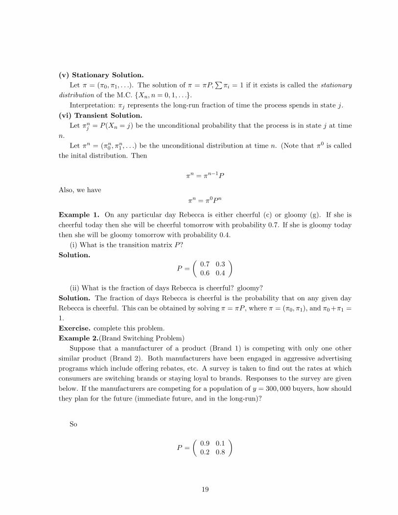
Example 1. On any particular day Rebecca is either cheerful (c) or gloomy (g). If she is

cheerful today then she will be cheerful tomorrow with probability 0.7. If she is gloomy today

then she will be gloomy tomorrow with probability 0.4.

(i) What is the transition matrix P?

Solution.

P =

(

0.7 0.3

0.6 0.4

)

(ii) What is the fraction of days Rebecca is cheerful? gloomy?

Solution. The fraction of days Rebecca is cheerful is the probability that on any given day

Rebecca is cheerful. This can be obtained by solving π = πP , where π = (π0, π1), and π0 +π1 =

1.

Exercise. complete this problem.

Example 2.(Brand Switching Problem)

Suppose that a manufacturer of a product (Brand 1) is competing with only one other

similar product (Brand 2). Both manufacturers have been engaged in aggressive advertising

programs which include offering rebates, etc. A survey is taken to find out the rates at which

consumers are switching brands or staying loyal to brands. Responses to the survey are given

below. If the manufacturers are competing for a population of y = 300, 000 buyers, how should

they plan for the future (immediate future, and in the long-run)?

So

P =

(

0.9 0.10.2 0.8

)

19

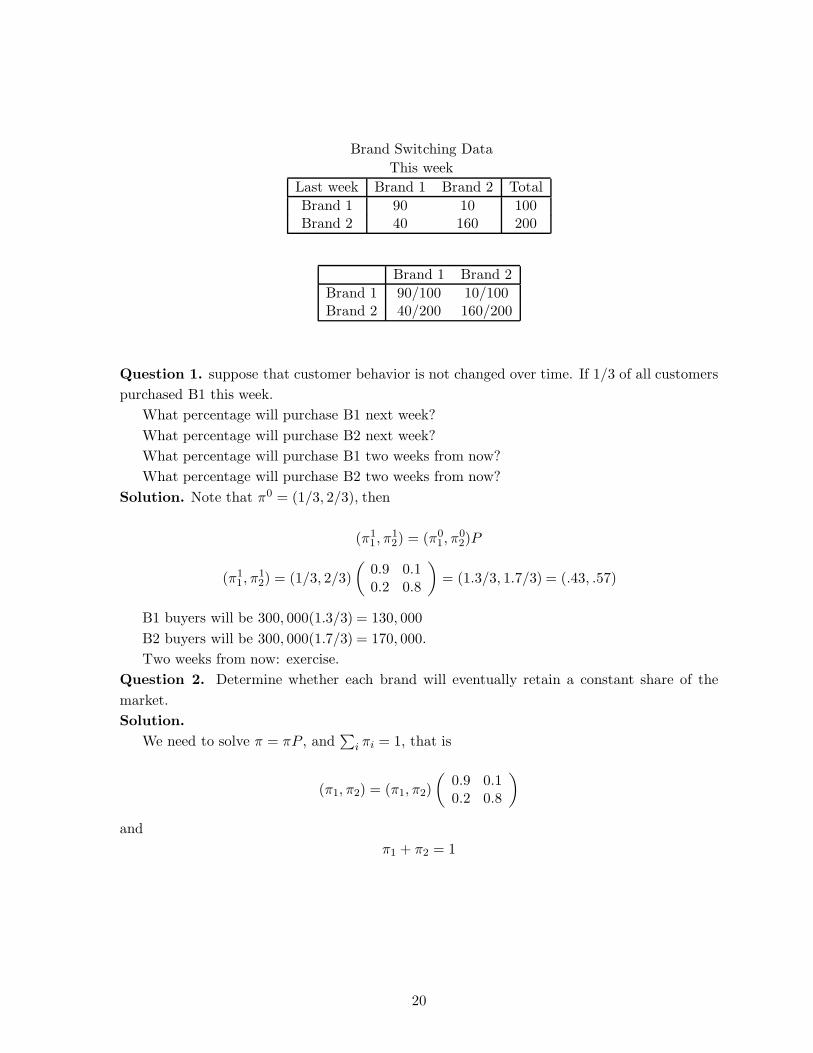
Brand Switching Data

This week

Last week Brand 1 Brand 2 Total

Brand 1 90 10 100Brand 2 40 160 200

Brand 1 Brand 2

Brand 1 90/100 10/100Brand 2 40/200 160/200

Question 1. suppose that customer behavior is not changed over time. If 1/3 of all customers

purchased B1 this week.

What percentage will purchase B1 next week?

What percentage will purchase B2 next week?

What percentage will purchase B1 two weeks from now?

What percentage will purchase B2 two weeks from now?

Solution. Note that π0 = (1/3, 2/3), then

(π11, π

12) = (π0

1, π02)P

(π11, π

12) = (1/3, 2/3)

(

0.9 0.10.2 0.8

)

= (1.3/3, 1.7/3) = (.43, .57)

B1 buyers will be 300, 000(1.3/3) = 130, 000

B2 buyers will be 300, 000(1.7/3) = 170, 000.

Two weeks from now: exercise.

Question 2. Determine whether each brand will eventually retain a constant share of the

market.

Solution.

We need to solve π = πP , and∑

i πi = 1, that is

(π1, π2) = (π1, π2)

(

0.9 0.10.2 0.8

)

and

π1 + π2 = 1

20

Matrix multiplication gives

π1 = 0.9π1 + 0.2π2

π2 = 0.1π1 + 0.8π2

π1 + π2 = 1

One equation is redundant. Choose the first and the third. we get

0.1π1 = 0.2π2 and π1 + π2 = 1

which gives

(π1, π2) = (2/3, 1/3)

Brand 1 will eventually capture two thirds of the market (200, 000) customers.

Camera Store Example (textbook)

Scenario. Suppose D1, D2, D3, . . . represent demands for weeks 1, 2, 3, . . .. Let X0 be

the # of cameras on hand at the end of week 0, i.e. beginning of week 1; and X1, X2, X3 = be

the # of cameras on hand at the end of week 1, 2, 3, . . . .

On Saturday night, the store places an order that is delivered on time Monday morning.

Ordering policy: (s,S) policy, i.e. order up to S if inventory level drops below s;

otherwise, do not order. In this example we have a (1, 3) policy.

Suppose D1, D2, D3 are iid

Xn+1 =

max (3− Dn+1), 0 if Xn < 1,max (Xn − Dn+1), 0, if Xn ≥ 1,

for all n = 0, 1, 2, . . ..

21

For n = 0, 1, 2, . . .,

(i) Xn = 0 or 1 or 2 or 3.

(ii) Integer state process

(iii) Finite state process

Remarks

(1) Xn+1 depends on Xn

(2) Xn+1 does not depend on Xn−1 directly i.e. it depends on Xn−1 only through Xn.

(3) If Dn+1 is known, Xn gives us enough information to determine Xn+1. (Markovian

Property).

RECALL: Markov Chains

A discrete time stochastic process is said to be a Markov chain if

PXn+1 = j|X0 = x0, X1 = x1, . . . , Xn−1 = xn−1, Xn = i= PXn+1 = j|Xn = i = PX1 = j|X0 = i,

for n = 0, 1, . . . and every sequence i, j, x0, x1, . . . , xn−1.

Definition. A stochastic process Xn (n = 0, 1, . . .) is said to be a finite state Markov chain

if it has

(1) A finite # of states

(2) The Markovian property

(3) Stationary transition probabilities

(4) A set of initial probabilities

π(0)i = PX0 = i for all i = 0, 1, . . . , m.

Example. (Inventory example)

One-step transition matrix (Stochastic Matrix)

P =

p00 p01 p02 p03

p10 p11 p12 p13

p20 p21 p22 p23

p30 p31 p32 p33

In general

P =

p00 p01 p0m

p10 p11 · · · p1m...

pm0 pm1 · · · pmm

pi,j ≥ 0 for all i, j = 0, 1, . . . , m.

22

m∑

j=0

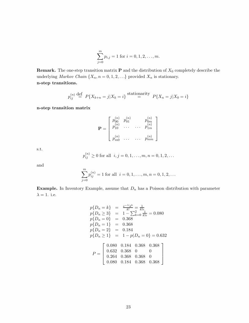
pi,j = 1 for i = 0, 1, 2, . . . , m.

Remark. The one-step transition matrix P and the distribution of X0 completely describe the

underlying Markov Chain Xn, n = 0, 1, 2, . . . provided Xn is stationary.

n-step transitions.

p(n)ij

def= PXk+n = j|Xk = i stationarity

= PXn = j|X0 = i

n-step transition matrix

P =

p(n)00 p

(n)01 p

(n)0m

p(n)10 . . . . . . p

(n)1m

p(n)m0 . . . . . . p

(n)mm

s.t.

p(n)ij ≥ 0 for all i, j = 0, 1, . . . , m, n = 0, 1, 2, . . .

andm

∑

j=0

p(n)ij = 1 for all i = 0, 1, . . . , m, n = 0, 1, 2, . . .

Example. In Inventory Example, assume that Dn has a Poisson distribution with parameter

λ = 1. i.e.

pDn = k = e−λλk

k! = 1k!e

pDn ≥ 3 = 1 − ∑2k=0

1k!e = 0.080

pDn = 0 = 0.368

pDn = 1 = 0.368pDn = 2 = 0.184

pDn ≥ 1 = 1 − p(Dn = 0 = 0.632

P =

0.080 0.184 0.368 0.368

0.632 0.368 0 00.264 0.368 0.368 00.080 0.184 0.368 0.368

23

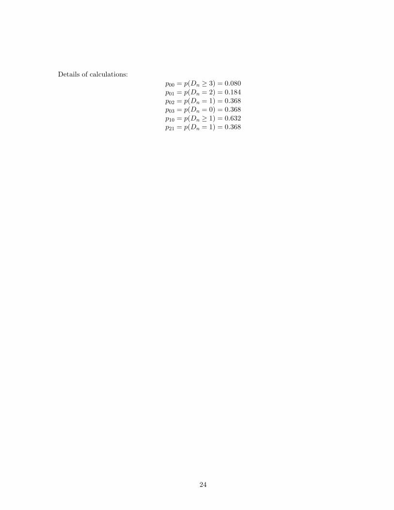
Details of calculations:

p00 = p(Dn ≥ 3) = 0.080

p01 = p(Dn = 2) = 0.184p02 = p(Dn = 1) = 0.368p03 = p(Dn = 0) = 0.368

p10 = p(Dn ≥ 1) = 0.632p21 = p(Dn = 1) = 0.368

24

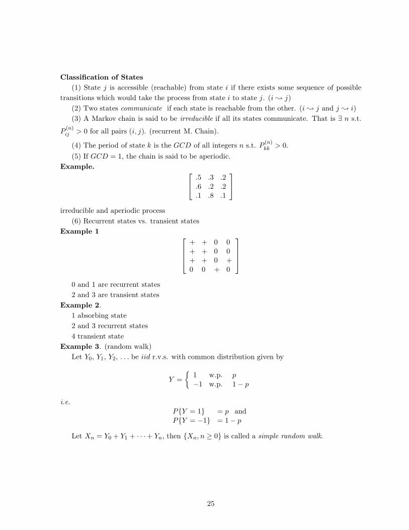
Classification of States

(1) State j is accessible (reachable) from state i if there exists some sequence of possible

transitions which would take the process from state i to state j. (i ; j)

(2) Two states communicate if each state is reachable from the other. (i ; j and j ; i)

(3) A Markov chain is said to be irreducible if all its states communicate. That is ∃ n s.t.

P(n)ij > 0 for all pairs (i, j). (recurrent M. Chain).

(4) The period of state k is the GCD of all integers n s.t. P(n)kk > 0.

(5) If GCD = 1, the chain is said to be aperiodic.

Example.

.5 .3 .2

.6 .2 .2

.1 .8 .1

irreducible and aperiodic process

(6) Recurrent states vs. transient states

Example 1

+ + 0 0

+ + 0 0+ + 0 +

0 0 + 0

0 and 1 are recurrent states

2 and 3 are transient states

Example 2.

1 absorbing state

2 and 3 recurrent states

4 transient state

Example 3. (random walk)

Let Y0, Y1, Y2, . . . be iid r.v.s. with common distribution given by

Y =

1 w.p. p

−1 w.p. 1 − p

i.e.

PY = 1 = p and

PY = −1 = 1 − p

Let Xn = Y0 + Y1 + · · ·+ Yn, then Xn, n ≥ 0 is called a simple random walk.

25

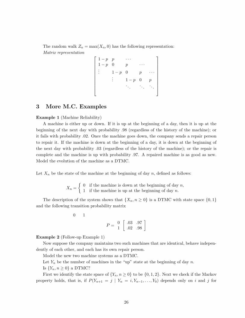
The random walk Zn = max(Xn, 0) has the following representation:

Matrix representation

1 − p p · · ·1 − p 0 p · · ·... 1− p 0 p · · ·

... 1 − p 0 p. . .

. . .. . .

3 More M.C. Examples

Example 1 (Machine Reliability)

A machine is either up or down. If it is up at the beginning of a day, then it is up at the

beginning of the next day with probability .98 (regardless of the history of the machine); or

it fails with probability .02. Once the machine goes down, the company sends a repair person

to repair it. If the machine is down at the beginning of a day, it is down at the beginning of

the next day with probability .03 (regardless of the history of the machine); or the repair is

complete and the machine is up with probability .97. A repaired machine is as good as new.

Model the evolution of the machine as a DTMC.

Let Xn be the state of the machine at the beginning of day n, defined as follows:

Xn =

0 if the machine is down at the beginning of day n,1 if the machine is up at the beginning of day n.

The description of the system shows that Xn, n ≥ 0 is a DTMC with state space 0, 1and the following transition probability matrix

0 1

P =01

[

.03 .97

.02 .98

]

Example 2 (Follow-up Example 1)

Now suppose the company maintains two such machines that are identical, behave indepen-

dently of each other, and each has its own repair person.

Model the new two machine systems as a DTMC.

Let Yn be the number of machines in the “up” state at the beginning of day n.

Is Yn, n ≥ 0 a DTMC?

First we identify the state space of Yn, n ≥ 0 to be 0, 1, 2. Next we check if the Markov

property holds, that is, if P (Yn+1 = j | Yn = i, Yn−1, . . . , Y0) depends only on i and j for

26

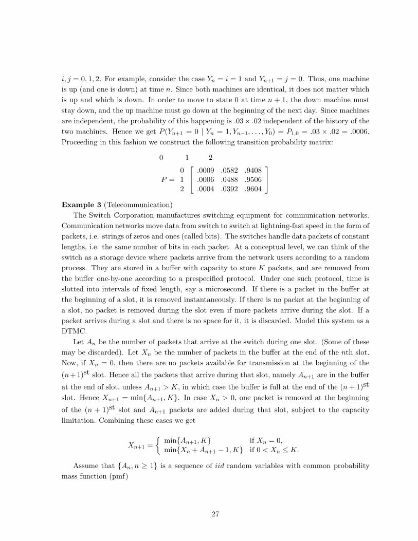
i, j = 0, 1, 2. For example, consider the case Yn = i = 1 and Yn+1 = j = 0. Thus, one machine

is up (and one is down) at time n. Since both machines are identical, it does not matter which

is up and which is down. In order to move to state 0 at time n + 1, the down machine must

stay down, and the up machine must go down at the beginning of the next day. Since machines

are independent, the probability of this happening is .03× .02 independent of the history of the

two machines. Hence we get P (Yn+1 = 0 | Yn = 1, Yn−1, . . . , Y0) = P1,0 = .03 × .02 = .0006.

Proceeding in this fashion we construct the following transition probability matrix:

0 1 2

P =01

2

.0009 .0582 .9408

.0006 .0488 .9506

.0004 .0392 .9604

Example 3 (Telecommunication)

The Switch Corporation manufactures switching equipment for communication networks.

Communication networks move data from switch to switch at lightning-fast speed in the form of

packets, i.e. strings of zeros and ones (called bits). The switches handle data packets of constant

lengths, i.e. the same number of bits in each packet. At a conceptual level, we can think of the

switch as a storage device where packets arrive from the network users according to a random

process. They are stored in a buffer with capacity to store K packets, and are removed from

the buffer one-by-one according to a prespecified protocol. Under one such protocol, time is

slotted into intervals of fixed length, say a microsecond. If there is a packet in the buffer at

the beginning of a slot, it is removed instantaneously. If there is no packet at the beginning of

a slot, no packet is removed during the slot even if more packets arrive during the slot. If a

packet arrives during a slot and there is no space for it, it is discarded. Model this system as a

DTMC.

Let An be the number of packets that arrive at the switch during one slot. (Some of these

may be discarded). Let Xn be the number of packets in the buffer at the end of the nth slot.

Now, if Xn = 0, then there are no packets available for transmission at the beginning of the

(n+1)st slot. Hence all the packets that arrive during that slot, namely An+1 are in the buffer

at the end of slot, unless An+1 > K, in which case the buffer is full at the end of the (n + 1)st

slot. Hence Xn+1 = minAn+1, K. In case Xn > 0, one packet is removed at the beginning

of the (n + 1)st slot and An+1 packets are added during that slot, subject to the capacity

limitation. Combining these cases we get

Xn+1 =

minAn+1, K if Xn = 0,

minXn + An+1 − 1, K if 0 < Xn ≤ K.

Assume that An, n ≥ 1 is a sequence of iid random variables with common probability

mass function (pmf)

27

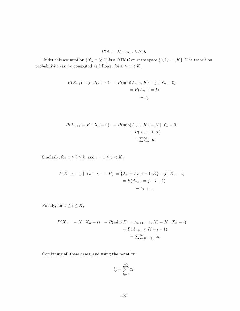
P (An = k) = ak, k ≥ 0.

Under this assumption Xn, n ≥ 0 is a DTMC on state space 0, 1, . . . , K. The transition

probabilities can be computed as follows: for 0 ≤ j < K,

P (Xn+1 = j | Xn = 0) = P (min(An+1, K = j | Xn = 0)

= P (An+1 = j)

= aj

P (Xn+1 = K | Xn = 0) = P (min(An+1, K = K | Xn = 0)

= P (An+1 ≥ K)

=∑∞

k=K ak

Similarly, for a ≤ i ≤ k, and i − 1 ≤ j < K,

P (Xn+1 = j | Xn = i) = P (minXn + An+1 − 1, K = j | Xn = i)

= P (An+1 = j − i + 1)

= aj−i+1

Finally, for 1 ≤ i ≤ K,

P (Xn+1 = K | Xn = i) = P (minXn + An+1 − 1, K) = K | Xn = i)

= P (An+1 ≥ K − i + 1)

=∑∞

k=K−i+1 ak

Combining all these cases, and using the notation

bj =

∞∑

k=j

ak

28

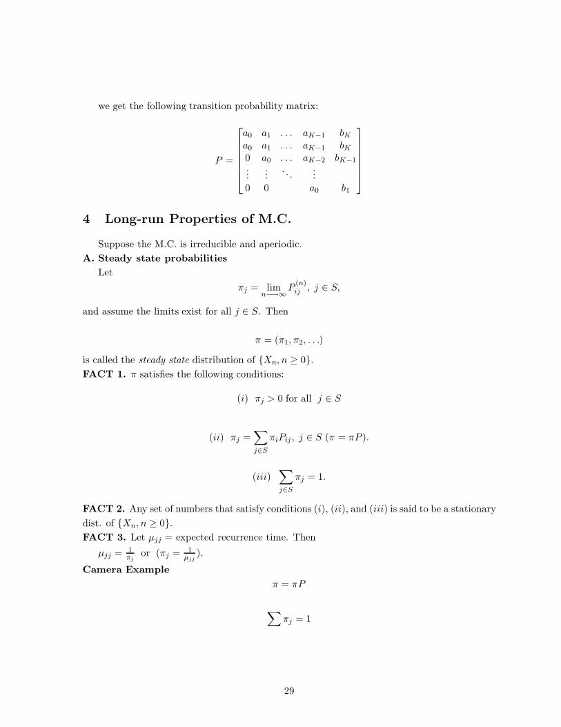
we get the following transition probability matrix:

P =

a0 a1 . . . aK−1 bK

a0 a1 . . . aK−1 bK

0 a0 . . . aK−2 bK−1...

.... . .

...

0 0 a0 b1

4 Long-run Properties of M.C.

Suppose the M.C. is irreducible and aperiodic.

A. Steady state probabilities

Let

πj = limn−→∞

P(n)ij , j ∈ S,

and assume the limits exist for all j ∈ S. Then

π = (π1, π2, . . .)

is called the steady state distribution of Xn, n ≥ 0.FACT 1. π satisfies the following conditions:

(i) πj > 0 for all j ∈ S

(ii) πj =∑

j∈S

πiPij , j ∈ S (π = πP ).

(iii)∑

j∈S

πj = 1.

FACT 2. Any set of numbers that satisfy conditions (i), (ii), and (iii) is said to be a stationary

dist. of Xn, n ≥ 0.FACT 3. Let µjj = expected recurrence time. Then

µjj = 1πj

or (πj = 1µjj

).

Camera Example

π = πP

∑

πj = 1

29

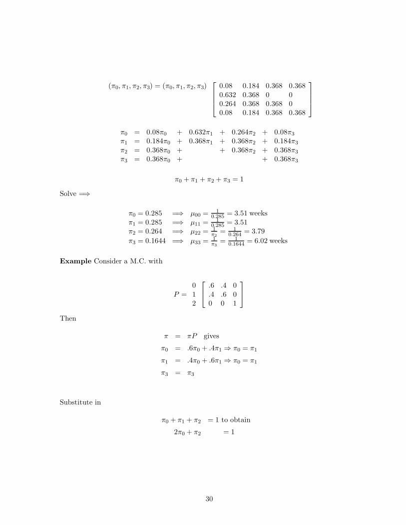
(π0, π1, π2, π3) = (π0, π1, π2, π3)

0.08 0.184 0.368 0.368

0.632 0.368 0 00.264 0.368 0.368 00.08 0.184 0.368 0.368

π0 = 0.08π0 + 0.632π1 + 0.264π2 + 0.08π3

π1 = 0.184π0 + 0.368π1 + 0.368π2 + 0.184π3

π2 = 0.368π0 + + 0.368π2 + 0.368π3

π3 = 0.368π0 + + 0.368π3

π0 + π1 + π2 + π3 = 1

Solve =⇒

π0 = 0.285 =⇒ µ00 = 10.285 = 3.51 weeks

π1 = 0.285 =⇒ µ11 = 10.285 = 3.51

π2 = 0.264 =⇒ µ22 = 1π2

= 10.264 = 3.79

π3 = 0.1644 =⇒ µ33 = 1π3

= 10.1644 = 6.02 weeks

Example Consider a M.C. with

P =

0

12

.6 .4 0

.4 .6 00 0 1

Then

π = πP gives

π0 = .6π0 + .4π1 ⇒ π0 = π1

π1 = .4π0 + .6π1 ⇒ π0 = π1

π3 = π3

Substitute in

π0 + π1 + π2 = 1 to obtain

2π0 + π2 = 1

30

Let π2 = α

2π0 = 1 − α

π0 =1 − α

2

Then

π =

(

1 − α

2,1− α

2, α

)

(valid for any 0 ≤ α ≤ 1.)

Therefore, the stationary distribution is not unique.

FACT If the steady state distribution exists, then it is unique and it satisfies

π = πP∑

πi = 1.

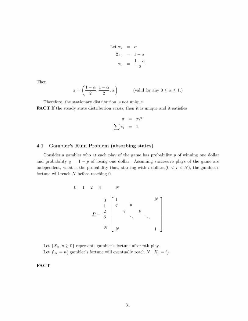
4.1 Gambler’s Ruin Problem (absorbing states)

Consider a gambler who at each play of the game has probability p of winning one dollar

and probability q = 1 − p of losing one dollar. Assuming successive plays of the game are

independent, what is the probability that, starting with i dollars,(0 < i < N ), the gambler’s

fortune will reach N before reaching 0.

0 1 2 3 N

P =

0

123

N

1 N

q pq p

. . .. . .

N 1

Let Xn, n ≥ 0 represents gambler’s fortune after nth play.

Let fiN = p gambler’s fortune will eventually reach N | X0 = i.

FACT

31

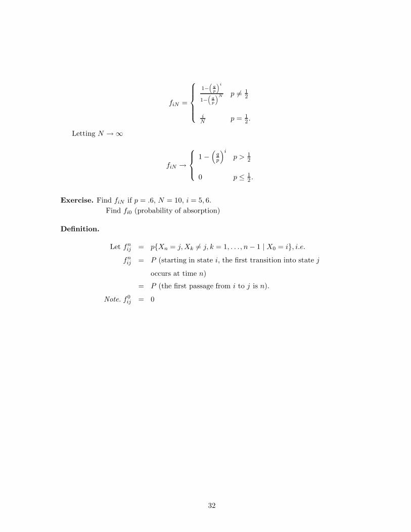
fiN =

1−(

q

p

)i

1−(

q

p

)N p 6= 12

iN p = 1

2 .

Letting N → ∞

fiN →

1 −(

qp

)ip > 1

2

0 p ≤ 12 .

Exercise. Find fiN if p = .6, N = 10, i = 5, 6.

Find fi0 (probability of absorption)

Definition.

Let fnij = pXn = j, Xk 6= j, k = 1, . . . , n − 1 | X0 = i, i.e.

fnij = P (starting in state i, the first transition into state j

occurs at time n)

= P (the first passage from i to j is n).

Note. f0ij = 0

32

Remark.

Let Yijr.v.= # of transitions made by the M.C. in going from state i to state j for the first

time

fnij = P(starting in state i, the first transition into state j occurs at time n)

(= first passage time from i to j)

Yii =recurrence time of state i .

Then fnij = PYij = n.

Definition.

Let fij =

∞∑

n=1

fnij

be the P (of ever making a transition into state j | given that the M.C. starts in i )

FACT.

fij > 0 (i 6= j) iff i → j.

33

Definition.

− state j is said to be recurrent if fjj =∞∑

n=1

fnjj = 1.

− state j is said to be transient if fjj =

∞∑

n=1

fnjj < 1.

− state j is said to be absorbing if fnjj = 1.

Remarks.

1. Suppose the M.C. starts in state i and i is recurrent. Then the M.C. will eventually

re-enter state i with prob. 1. It can be shown that state i will be visited infinitely often

(fij = 1).

2. Suppose state i is transient. Then

1− fii = Prob. state i will never be visited again.

fii = Prob. state i will be visited again.

=⇒ Starting in state i, the # of visits to state i is a random variable with a geometric

distribution, f(n) = fnii(1− fii) with a finite mean = 1

1−fii.

3. Let

In =

1 if Xn = i0 if Xn 6= i, then

∞∑

n=0

In = # of periods the M.C. is in state i.

E

[

∞∑

n=0

In | X0 = i

]

=

∞∑

n=0

E [In | X0 = i]

=

∞∑

n=0

P (Xn = i | X0 = i)

=

∞∑

n=0

pnii

34

Proposition

− state j is recurrent iff

∞∑

n=0

pnjj = ∞.

− state j is transient iff

∞∑

n=1

pnjj < ∞.

− state j is absorbing iff pnjj = 1.

Corollary

1. A transient state can be visited only a finite number of times.

2. A finite state M.C. cannot have all its states transients.

Calculating f(n)ij recursively

Note that

p(n)ij =

n∑

k=1

f(k)ij p

(n−k)jj

=

n−1∑

k=1

f(k)ij p

(n−k)jj + f

(n)ij p

(0)jj (note: p

(0)jj = 1 )

FACT

f(n)ij = p

(n)ij −

n−1∑

k=1

f(k)ij p

(n−k)jj

Example 1

f(1)ij = p

(1)ij = pij

f(2)ij = p

(2)ij − f

(1)ij pjj

...

f(n)ij = p

(n)ij − f

(1)ij p

(n−1)jj − f

(2)ij p

(n−2)jj · · · − f

(n−1)ij pjj

35

Example 2 for i = j

f(1)jj = pjj

f(2)jj = p

(2)jj − f

(1)jj pjj

...

f(n)jj = p

(n)jj − f

(1)jj p

(n−1)jj − f

(2)jj p

(n−2)jj − · · · − f

(n−1)jj pjj

Corollary

If i is recurrent, and i ⇐⇒ j, then state j is recurrent.

Proof

Since i ⇐⇒ j, there exists k and m s.t.

pkij > 0 and pm

ij > 0. Now, for any n (integer)

pm+n+kij ≥ pm

jipniip

kij

∞∑

n=1

pm+n+kjj ≥

∞∑

n=1

pmjip

niip

kij

= pmjip

kij

∞∑

n=1

pnii

= ∞

because i is recurrent, pmji > 0 and pk

ij > 0.

Therefore j is also recurrent.

Recall.

Yij = first passage time from i to j

Yii = recurrence time of state i

D.F. of Yij is given by fnij = P (Yij = n)

(we also defined fij =

∞∑

n=1

fnij).

36

Now, let

µij = E[Yij] =

∞∑

n=1

nf(n)ij

= expected first passage time from i to j

µjj = mean recurrence time

= expected number of transitions to return to state j

FACT

µjj =

∞ if j is transient (fjj < 1)

∑∞n=1 nfn

jj if j is recurrent (fjj = 1)

Definition

Let j be a recurrent state (equiv. fjj = 1), then

state j is positive recurrent if µjj < +∞, andstate j is null recurrent if µjj = ∞.

FACT Suppose all states are recurrent. Then

µij satisfies the following equations

µij = 1 +∑

k 6=j

pikµkj

Flow Balance Equations

π = πP ⇐⇒πj =

∑

i

πipij ⇐⇒

πj

∑

k

pjk =∑

i

πipij

Prob. flow out = Prob. flow in

37

πj

∑

k

pjk =∑

i

πipij

πj =∑

i

πipij (∗)

verification of (*).

Let

C(i, j; n) = number of transition from i to j during [0,n]

Y (i, n) = time in state i during [0, n].

pij = limn→∞

C(i, j; n)

Y (i, n)

πi = limn→∞

Y (i, n)

n∑

i

πipij =∑

i

limn→∞

Y (i, n)

n

C(i, j; n)

Y (i, n)

= limn→∞

∑

i

C(i, j; n)

n

= limn→∞

∑

i C(i, j; n)

n

= limn→∞

Y (j, n)

n= πj

Note.

πipij = limn→∞

Y (i, n)

n

C(i, j; n)

Y (i, n)= lim

n→∞

C(i, j; n)

n= rate from i to j.

4.2 Sums of Independent, Identically Distributed, Random Variables

Let Yi, i = 1, 2, . . . , be iid with

PYi = j = aj , j ≥ 0

∞∑

j=0

aj = 1.

38

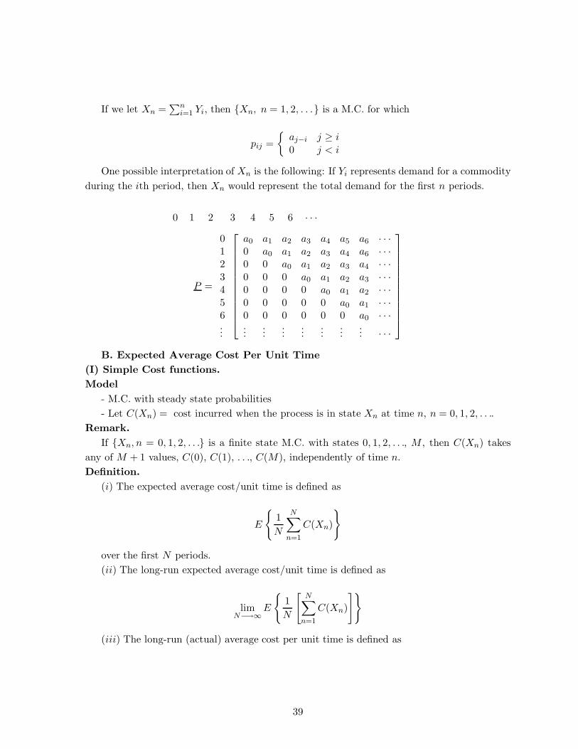
If we let Xn =∑n

i=1 Yi, then Xn, n = 1, 2, . . . is a M.C. for which

pij =

aj−i j ≥ i

0 j < i

One possible interpretation of Xn is the following: If Yi represents demand for a commodity

during the ith period, then Xn would represent the total demand for the first n periods.

0 1 2 3 4 5 6 · · ·

P =

012

34

56...

a0 a1 a2 a3 a4 a5 a6 · · ·0 a0 a1 a2 a3 a4 a6 · · ·0 0 a0 a1 a2 a3 a4 · · ·0 0 0 a0 a1 a2 a3 · · ·0 0 0 0 a0 a1 a2 · · ·0 0 0 0 0 a0 a1 · · ·0 0 0 0 0 0 a0 · · ·...

......

......

...... · · ·

B. Expected Average Cost Per Unit Time

(I) Simple Cost functions.

Model

- M.C. with steady state probabilities

- Let C(Xn) = cost incurred when the process is in state Xn at time n, n = 0, 1, 2, . . ..

Remark.

If Xn, n = 0, 1, 2, . . . is a finite state M.C. with states 0, 1, 2, . . ., M , then C(Xn) takes

any of M + 1 values, C(0), C(1), . . ., C(M), independently of time n.

Definition.

(i) The expected average cost/unit time is defined as

E

1

N

N∑

n=1

C(Xn)

over the first N periods.

(ii) The long-run expected average cost/unit time is defined as

limN−→∞

E

1

N

[

N∑

n=1

C(Xn)

]

(iii) The long-run (actual) average cost per unit time is defined as

39

limN−→∞

1

N

N∑

n=1

C(Xn)

FACT. For almost all paths of the M.C.

(ii) = (iii) =

M∑

j=0

πjC(j).

i.e.

limN−→∞

E

[

1

N

N∑

n=1

C(Xn)

]

= limN−→∞

1

N

N∑

n=1

C(Xn) =

M∑

j=0

C(j)πj

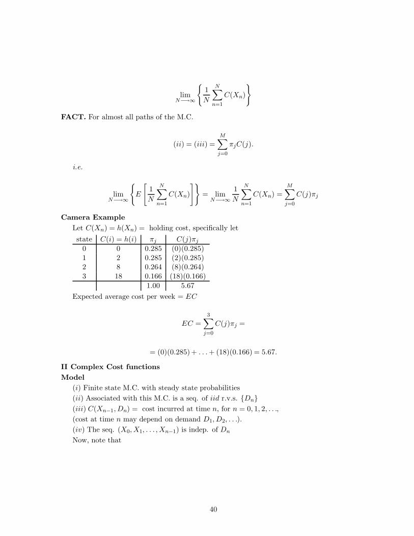
Camera Example

Let C(Xn) = h(Xn) = holding cost, specifically let

state C(i) = h(i) πj C(j)πj

0 0 0.285 (0)(0.285)

1 2 0.285 (2)(0.285)2 8 0.264 (8)(0.264)

3 18 0.166 (18)(0.166)

1.00 5.67

Expected average cost per week = EC

EC =

3∑

j=0

C(j)πj =

= (0)(0.285)+ . . . + (18)(0.166) = 5.67.

II Complex Cost functions

Model

(i) Finite state M.C. with steady state probabilities

(ii) Associated with this M.C. is a seq. of iid r.v.s. Dn(iii) C(Xn−1, Dn) = cost incurred at time n, for n = 0, 1, 2, . . .,

(cost at time n may depend on demand D1, D2, . . .).

(iv) The seq. (X0, X1, . . . , Xn−1) is indep. of Dn

Now, note that

40

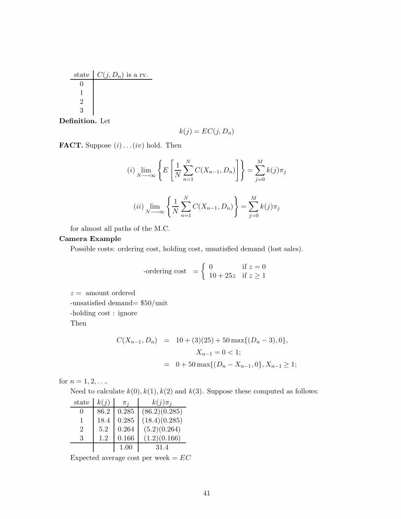
state C(j, Dn) is a rv.

01

23

Definition. Let

k(j) = EC(j, Dn)

FACT. Suppose (i) . . .(iv) hold. Then

(i) limN−→∞

E

[

1

N

N∑

n=1

C(Xn−1, Dn)

]

=

M∑

j=0

k(j)πj

(ii) limN−→∞

1

N

N∑

n=1

C(Xn−1, Dn)

=

M∑

j=0

k(j)πj

for almost all paths of the M.C.

Camera Example

Possible costs: ordering cost, holding cost, unsatisfied demand (lost sales).

-ordering cost =

0 if z = 010 + 25z if z ≥ 1

z = amount ordered

-unsatisfied demand= $50/unit

-holding cost : ignore

Then

C(Xn−1, Dn) = 10 + (3)(25) + 50 max(Dn − 3), 0,Xn−1 = 0 < 1;

= 0 + 50 max(Dn − Xn−1, 0, Xn−1 ≥ 1;

for n = 1, 2, . . ..

Need to calculate k(0), k(1), k(2) and k(3). Suppose these computed as follows:

state k(j) πj k(j)πj

0 86.2 0.285 (86.2)(0.285)

1 18.4 0.285 (18.4)(0.285)2 5.2 0.264 (5.2)(0.264)

3 1.2 0.166 (1.2)(0.166)

1.00 31.4

Expected average cost per week = EC

41

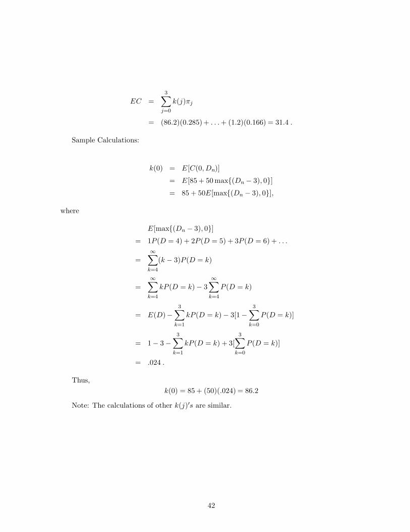
EC =

3∑

j=0

k(j)πj

= (86.2)(0.285)+ . . . + (1.2)(0.166) = 31.4 .

Sample Calculations:

k(0) = E[C(0, Dn)]

= E[85 + 50 max(Dn − 3), 0]= 85 + 50E[max(Dn − 3), 0],

where

E[max(Dn − 3), 0]= 1P (D = 4) + 2P (D = 5) + 3P (D = 6) + . . .

=

∞∑

k=4

(k − 3)P (D = k)

=

∞∑

k=4

kP (D = k)− 3

∞∑

k=4

P (D = k)

= E(D)−3

∑

k=1

kP (D = k)− 3[1−3

∑

k=0

P (D = k)]

= 1− 3 −3

∑

k=1

kP (D = k) + 3[

3∑

k=0

P (D = k)]

= .024 .

Thus,

k(0) = 85 + (50)(.024) = 86.2

Note: The calculations of other k(j)′s are similar.

42

Chapter 4

Poisson and Markov Processes

Contents.

The Poisson Process

The Markov Process

The Birth-Death Process

1 The Poisson Process

A stochastic process is a collection of random variables that describes the evolution of some

system over time.

A stochastic process N (t), t ≥ 0 is said to be a counting process if N (t) represents the

total number of events that have occurred up to time t. A counting process must satisfy:

(i) N (t) ≥ 0

(ii) N (t) is integer valued.

(iii) If s < t, then N (s) ≤ N (t).

(iv) For s < t, N (t)− N (s) counts the number of events that have occurred in the interval

(s, t].

Definition 1.

(i) A counting process is said to have independent increments if the number of events that

occur in disjoint time intervals are independent. For example, N (t + s) − N (t) and N (t) are

independent.

(ii) A counting process is said to have stationary increments if the distribution of the number

of events that occur in any time interval depends only on the length of that interval. For

example, N (t + s) − N (t) and N (s) have the same distribution.

Definition 2. The counting process N (t), t ≥ 0 is said to be a Poisson process having rate

λ, λ > 0, if:

(i) N (0) = 0.

(ii) The process has independent increments.

43

(iii) The number of events in any interval of length t is Poisson distributed with mean λt.

That is for all s, t ≥ 0,

PN (t + s) − N (s) = n =e−λt(λt)n

n!, n = 0, 1, . . . .

Interevents: Consider a Poisson process. Let X1 be the time of the first event. For n ≥ 1, let

Xn denote the time between the (n − 1)st and nth event. The sequence Xn, n ≥ 1 is called

the sequence of interarrival times.

Proposition 1.1 The rvs Xn, n = 1, 2, . . . are iid exponential rvs having mean 1/λ.

Remark. A process N (t), t ≥ 0 is said to be a renewal process if the interevent rvs Xn, n =

1, 2, . . . are iid with some distribution function F .

Definition 3. The counting process N (t), t ≥ 0 is said to be a Poisson process having rate

λ, λ > 0, if:

(i) N (0) = 0;

(ii) N (t), t ≥ 0 has stationary indepedent increments

(iii) P (N (h) = 1) = λh + o(h)

(iv) P (N (h) ≥ 2) = o(h)

Remark. The above fact implies that P (N (h) = 0) = 1 − λh + o(h)

FACT. Definitions 2 and 3 are equivalent.

Proof. Omitted.

Properties

(i) The Poisson process has stationary increments.

(ii) E[N (t)] = λt

(iii) For s ≤ t

PX1 < s|N (t) = 1 =s

t.

That is the conditional time until the first event is uniformly distributed.

(iv) The Poisson process possesses the lack of memory property

(v) For a Poisson Process N (t), t ≥ 0 with rate λ,

P (N (t) = 0) = e−λt; and

P (N (t) = k) =e−λt(λt)k

k!, k = 0, 1, . . . .

(vi) Merging two independent Poisson processes with rates λ1 and λ2 results is a Poisson

process with rate λ1 + λ2.

44

(vii) Splitting a Poisson process with rate λ where the splitting mechanism is memoryless

(Bernoulli) with parameter p , results in two independent Poisson processes with rates λp and

λ(1− p) respectively.

Example Customers arrive in a certain store according to a Poisson process with mean rate

λ = 4 per hour. Given that the store opens at 9 : 00am,

(i) What is the probability that exactly one customer arrives by 9 : 30am?

Solution. Time is measured in hours starting at 9 : 00am.

P (N (0.5) = 1) = e−4(0.5)4(0.5)/1! = 2e−2

(ii) What is the probability that a total of five customers arrive by 11 : 30am?

Solution.

P (N (2.5) = 5) = e−4(2.5)[4(2.5)]5/5! = 104e−10/12

(iii) What is the probability that exactly one customer arrives between 10 : 30am and

11 : 00am?

Solution.

P (N (2)− N (1.5) = 1) = P (N (0.5) = 1)

= e−4(0.5)4(0.5)/1! = 2e−2

2 Markov Process

Definition. A continuous-time stochastic process X(t), t ≥ 0 with integer state space is said

to be a Markov process (M.P.) if it satisfies the Markovian property, i.e.

P (X(t + h) = j|X(t) = i, X(u) = x(u), 0 ≤ u < t)

= P (X(t + h) = j|X(t) = i)

for all t, h ≥ 0, and non-negative integers i, j, x(u)0 ≤ u < t.

Definition. A Markov process X(t), t ≥ 0 is said to have stationary (time-homogeneous)

transition probabilities if P (X(t + h) = j|X(t) = i) is independent of t, i.e.

P (X(t + h) = j|X(t) = i) = P (X(h) = j|X(0) = i) ≡ pij(h) .

Remarks A MP is a stochastic process that moves from one state to another in accordance

with a MC, but the amount of time spent in each state is exponentially distributed.

Example. Suppose a MP enters state i at some time, say 0, and suppose that the process does

not leave state i (i.e. a transition does not occur) during the next 10 minutes. What is the

probability that the process will not leave state i during the next 5 minutes?

45

Answer. Since the MP is in state i at time 10, it follows by the Markovian property, that

P (Ti > 15|Ti > 10) = P (Ti > 5) = e−5αi ,

where αi is the transition rate out of state i.

FACT. Ti is exponentially distributed with rate, say αi. That is P (Ti > t) = e−αit.

Remarks.

(i) pij(h) are called the transition probabilities for the MP.

(ii) In a MP, times between transitions are exponentially distributed, possibly with different

parameters.

(iii) A M.P. is characterized by its initial distribution and its transition matrix.

FACT. Let Ti be the time that the MP stays in state i before making a transition into a

different state. Then

P (Ti > t + h|Ti > t) = P (Ti > h) .

Proof. Follows from the Markovian property.

2.1 Rate Properties of Markov Processes

Recall

pij(h) = P (X(t + h) = j | X(t) = i)

Lemma

The transition rates (intensities) are given by

(i) qij = limh−→0

pij(h)

h, i 6= j

(ii) qi = limh−→0

1 − pij(h)

h, i ∈ S.

Remarks

(i) qi =∑

i6=j

qij

(ii) pij =qij

∑

j 6=i qij

46

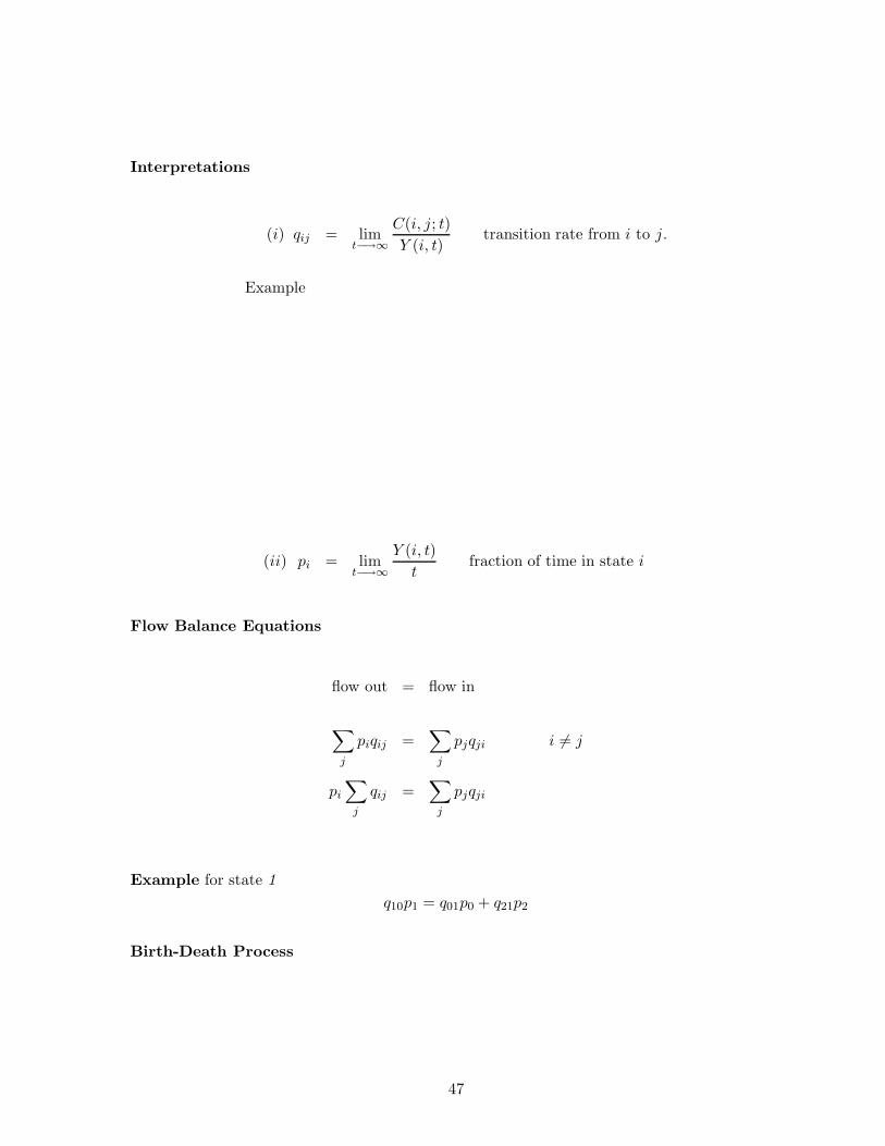
Interpretations

(i) qij = limt−→∞

C(i, j; t)

Y (i, t)transition rate from i to j.

Example

(ii) pi = limt−→∞

Y (i, t)

tfraction of time in state i

Flow Balance Equations

flow out = flow in

∑

j

piqij =∑

j

pjqji i 6= j

pi

∑

j

qij =∑

j

pjqji

Example for state 1

q10p1 = q01p0 + q21p2

Birth-Death Process

47

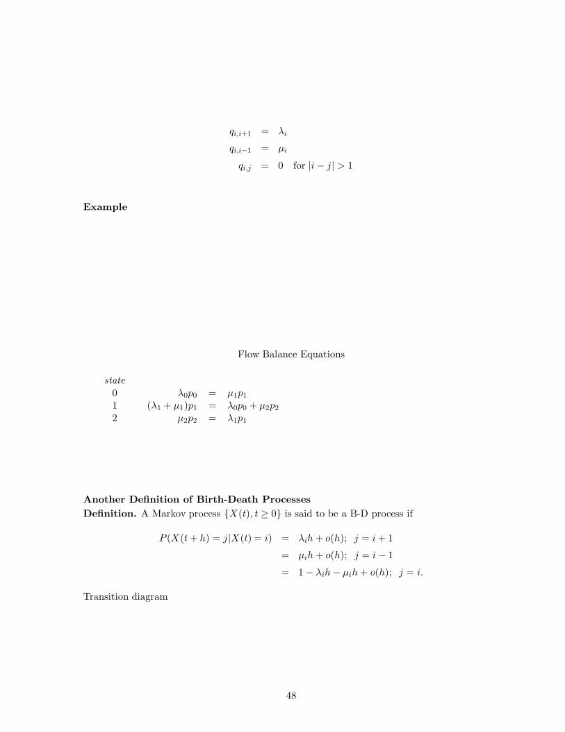
qi,i+1 = λi

qi,i−1 = µi

qi,j = 0 for |i − j| > 1

Example

Flow Balance Equations

state

0 λ0p0 = µ1p1

1 (λ1 + µ1)p1 = λ0p0 + µ2p2

2 µ2p2 = λ1p1

Another Definition of Birth-Death Processes

Definition. A Markov process X(t), t ≥ 0 is said to be a B-D process if

P (X(t + h) = j|X(t) = i) = λih + o(h); j = i + 1

= µih + o(h); j = i − 1

= 1 − λih − µih + o(h); j = i.

Transition diagram

48

Chapter 5

Queueing Models I

Contents.

Terminology

The Birth-Death Process

Models Based on the B-D Process

1 Terminology

Calling population. Total number of distinct potential arrivals (The size of the calling

population may be assumed to be finite (limited) or infinite (unlimited).

Arrivals. Let

A(t) := # of arrivals during [0, t]

λ := limt→∞A(t)

t (Mean arrival rate)1λ = Mean time between arrivals

Service times. Time it takes to process a job. Let distribution of service times has mean 1/µ,

i.e. µ is the mean service rate.

Queue discipline. FCFS, LCFS, Processor sharing (PS), Round robin (RR), SIRO, SPT,

priority rules, etc.

Number of servers. single or multiple servers (c = # of servers)

Waiting room. Finite vs infinite (Use K for finite waiting room)

Notation.

A/B/c/K/N (Kendall’s notation)

A: describes the arrival process

B: describes the service time distribution

c: number of servers

K: buffer size

N: size of the calling population

49

* A and B may be replaced by

M: Markovian or memoryless

D: Deterministic

Ek : Erlang distribution

G: General (usually the mean and variance are known)

Examples.

M/M/1;

M/M/2/5/20;

M/E3/1;

G/G/1.

M/M/1 queue.

(i) Time between arrivals are iid and exponential, i.e.

f(t) = λe−λt λ, t > 0;

= 0 otherwise.

(ii) Service times are iid and exponential, i.e.

g(t) = µe−µt µ, t > 0 ;

= 0 otherwise.

(iii) There is one server, infinite waiting room, and infinite calling population.

(iv) System is in statistical equilibrium (steady state) and stable

(v) Stability condition: ρ = λµ < 1.

Steady State Conditions.

Let X(t) = # of customers in system at time t. Then X(t), t ≥ 0 is a stochastic process.

We are interested in X(t), t ≥ 0 when

(i) it is a birth-death process

(ii) it has reached steady state (or stationarity) (i.e. the process has been evolving for a

long time)

Performance measures.

L = expected (mean) number of customers in the system

Lq = expected (mean) queue length (excluding customers in service)

W = expected (mean) time in system per arrival

Wq = expected (mean) time in queue per arrival

I = expected (mean) idle time per server

B = expected (mean) busy time per server

Pn, n ≥ 0 = distribution of number of customers in system

T = waiting time is system (including service time) for each arrival (random variable)

50

Tq = waiting time is queue , excluding service time, (delay) for each arrival (random variable)

P (T ≥ t) = distribution of waiting times

Percentiles

General Relations.

(i) Little’s formula:

L = λW

Lq = λWq

(ii)

W = Wq +1

µ

(iii) For systems that obey Little’s law

L = Lq +λ

µ

(iv) Single server

L = Lq + (1− P0)

Example. If λ is the arrival rate in a transmission line, Nq is the average number of packets

waiting in queue (but not under transmission), and Wq is the average time spent by a packet

waiting in queue (not including transmission time), Little’s formula gives

Nq = λWq .

Moreover, if S is the average transmission time, then Little’s formula gives the average number

of packets under transmission as

ρ = λS .

Since at most one packet can be under transmission, ρ is also the line’s utilization factor, i.e.,

the proportion of time that the line is busy transmitting packets.

2 The Birth-Death Process

Flow balance diagram

Flow Balance Equations.

First we write the global balance equations using the principle of flow balance.

Probability Flow out = Probability Flow in

51

Flow out = Flow in

λ0P0 = µ1P1

λ1P1 + µ1P1 = λ0P0 + µ2P2

λ2P2 + µ2P2 = λ1P1 + µ3P3

...

λkPk + µkPk = λk−1Pk−1 + µk+1Pk+1

...

Rewrite as

λ0P0 = µ1P1

λ1P1 = µ2P2

λ2P2 = µ3P3

...

λkPk = µk+1Pk+1

...

More compactly,

λnPn = µn+1Pn+1 , n = 0, 1, 2 . . . . (5.1)

Equations (5.1) are called local (detailed) balance equations.

Solve (5.1) recursively to obtain

P1 =λ0

µ1P0

P2 =λ1

µ2P1 =

λ0λ1

µ1µ2P0

P3 =λ2

µ3P2 =

λ0λ1λ2

µ1µ2µ3P0

...

So that

Pn =λ0λ1 · · ·λn−1

µ1µ2 · · ·µnP0 , (5.2)

for all n = 0, 1, 2 . . ..

Assumption. Pn, n = 0, 1, 2 . . . exist and∑∞

n=0 Pn = 1.

52

Let Cn =λ0λ1···λn−1

µ1µ2···µn, then (5.2) may be written as

Pn = CnP0 , n = 0, 1, 2 . . . .

Therefore, P0 + P1 + P2 + . . . = 1 imply

[1 + C1 + C2 + . . .]P0 = 1

P0 =1

1 +∑∞

k=1 Ck

=1

1 +∑∞

k=1

∏kj=1

λj−1

µj

Stability. A queueing system (B-D process) is stable if P0 > 0 (What happens if P0 = 0?) or

1 +

∞∑

k=1

k∏

j=1

λj−1

µj< ∞

Assuming stability,

P0 =1

1 +∑∞

k=1

∏kj=1

λj−1

µj

(5.3)

Pn = (

n∏

j=1

λj−1

µj)P0 , n = 1, 2 . . . . (5.4)

3 Models Based on the B-D Process

4 M/M/1 Model

Here we consider an M/M/1 single server Markovian model.

λj = λ , j = 0, 1, 2 . . .

µj = µ , j = 1, 2 . . .

Stability. Let ρ = λµ . Then

1 +

∞∑

k=1

ρk =

∞∑

k=0

ρk

=1

1− ρif ρ < 1 .

53

Therefore P0 = 1 − ρ and Pn = ρn(1− ρ). That is

Pn = ρn(1 − ρ) , n = 0, 1, 2 . . . (5.5)

Remark. (i) ρ is called the traffic intensity or utilization factor.

(ii) ρ < 1 is called the stability condition.

Measures of Performance.

L :=

∞∑

n=0

nPn =ρ

1 − ρ=

λ

µ − λ

Lq :=

∞∑

n=1

(n − 1)Pn =ρ2

1 − ρ=

λ2

µ(µ − λ)

W =1

µ − λ

Wq =λ

µ(µ − λ)

U = 1 − P0 = ρ

I = 1 − ρ

P (X ≥ k) = ρk

Barbershop Example.

- One barber, no appointments, FCFS

- Busy hours or Saturdays

- Arrivals follow a Poisson process with mean arrival rate of 5.1 customers per hour

- Service times are exponential with mean service time of 10 minutes.

(i) Can you model this system as an M/M/1 queue?

Solution. Yes, with

λ = 5.1 arrivals per hour1µ = 10 min, i.e µ = 1/10 per min = 6 per hour

54

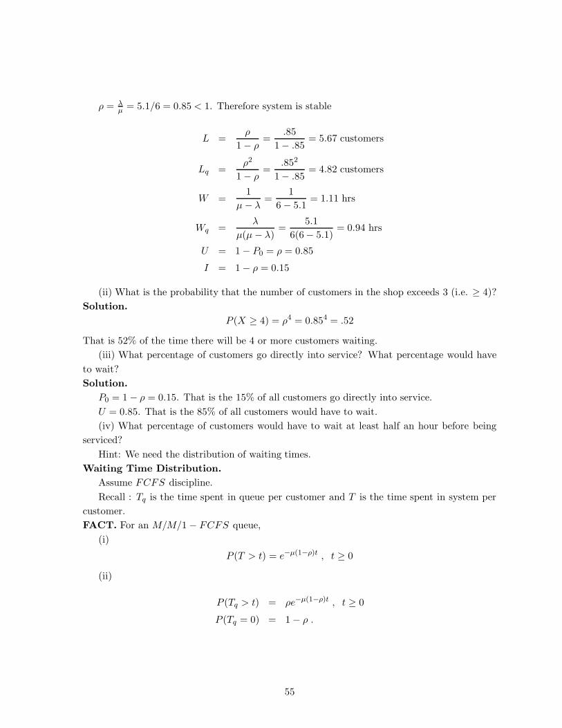
ρ = λµ = 5.1/6 = 0.85 < 1. Therefore system is stable

L =ρ

1 − ρ=

.85

1− .85= 5.67 customers

Lq =ρ2

1 − ρ=

.852

1− .85= 4.82 customers

W =1

µ − λ=

1

6 − 5.1= 1.11 hrs

Wq =λ

µ(µ − λ)=

5.1

6(6− 5.1)= 0.94 hrs

U = 1 − P0 = ρ = 0.85

I = 1 − ρ = 0.15

(ii) What is the probability that the number of customers in the shop exceeds 3 (i.e. ≥ 4)?

Solution.

P (X ≥ 4) = ρ4 = 0.854 = .52

That is 52% of the time there will be 4 or more customers waiting.

(iii) What percentage of customers go directly into service? What percentage would have

to wait?

Solution.

P0 = 1 − ρ = 0.15. That is the 15% of all customers go directly into service.

U = 0.85. That is the 85% of all customers would have to wait.

(iv) What percentage of customers would have to wait at least half an hour before being

serviced?

Hint: We need the distribution of waiting times.

Waiting Time Distribution.

Assume FCFS discipline.

Recall : Tq is the time spent in queue per customer and T is the time spent in system per

customer.

FACT. For an M/M/1 − FCFS queue,

(i)

P (T > t) = e−µ(1−ρ)t , t ≥ 0

(ii)

P (Tq > t) = ρe−µ(1−ρ)t , t ≥ 0

P (Tq = 0) = 1 − ρ .

55

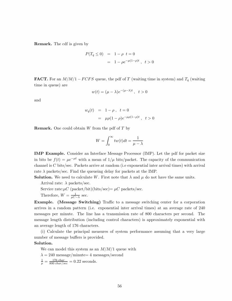
Remark. The cdf is given by

P (Tq ≤ 0) = 1 − ρ t = 0

= 1 − ρe−µ(1−ρ)t , t > 0

FACT. For an M/M/1−FCFS queue, the pdf of T (waiting time in system) and Tq (waiting

time in queue) are

w(t) = (µ − λ)e−(µ−λ)t , t > 0

and

wq(t) = 1− ρ , t = 0

= µρ(1− ρ)e−µρ(1−ρ)t , t > 0

Remark. One could obtain W from the pdf of T by

W =

∫ ∞

0tw(t)dt =

1

µ − λ

IMP Example. Consider an Interface Message Processor (IMP). Let the pdf for packet size

in bits be f(t) = µe−µt with a mean of 1/µ bits/packet. The capacity of the communication

channel is C bits/sec. Packets arrive at random (i.e exponential inter arrival times) with arrival

rate λ packets/sec. Find the queueing delay for packets at the IMP.

Solution. We need to calculate W . First note that λ and µ do not have the same units.

Arrival rate: λ packets/sec.

Service rate:µC (packet/bit)(bits/sec)= µC packets/sec.

Therefore, W = 1µC−λ sec.

Example. (Message Switching) Traffic to a message switching center for a corporation

arrives in a random pattern (i.e. exponential inter arrival times) at an average rate of 240

messages per minute. The line has a transmission rate of 800 characters per second. The

message length distribution (including control characters) is approximately exponential with

an average length of 176 characters.

(i) Calculate the principal measures of system performance assuming that a very large

number of message buffers is provided.

Solution.

We can model this system as an M/M/1 queue with

λ = 240 message/minute= 4 messages/second1µ = 176 char

800 char/sec= 0.22 seconds.

56

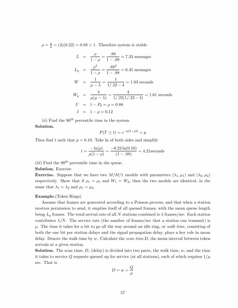
ρ = λµ = (4)(0.22) = 0.88 < 1. Therefore system is stable

L =ρ

1 − ρ=

.88

1 − .88= 7.33 messages

Lq =ρ2

1 − ρ=

.882

1 − .88= 6.45 messages

W =1

µ − λ=

1

1/.22− 4= 1.83 seconds

Wq =λ

µ(µ − λ)=

4

1/.22(1/.22− 4)= 1.61 seconds

U = 1 − P0 = ρ = 0.88

I = 1 − ρ = 0.12

(ii) Find the 90th percentile time in the system.

Solution.

P (T ≥ t) = e−µ(1−ρ)t = p

Then find t such that p = 0.10. Take ln of both sides and simplify

t =− ln(p)

µ(1 − ρ)=

−0.22 ln(0.10)

(1 − .88)= 4.21seconds

(iii) Find the 90th percentile time in the queue.

Solution. Exercise

Exercise. Suppose that we have two M/M/1 models with parameters (λ1, µ1) and (λ2, µ2)

respectively. Show that if ρ1 = ρ1 and W1 = W2, then the two models are identical, in the

sense that λ1 = λ2 and µ1 = µ2.

Example.(Token Rings)

Assume that frames are generated according to a Poisson process, and that when a station

receives permission to send, it empties itself of all queued frames, with the mean queue length

being Lq frames. The total arrival rate of all N stations combined is λ frames/sec. Each station

contributes λ/N . The service rate (the number of frames/sec that a station can transmit) is

µ. The time it takes for a bit to go all the way around an idle ring, or walk time, consisting of

both the one bit per station delays and the signal propagation delay, plays a key role in mean

delay. Denote the walk time by w. Calculate the scan time,D, the mean interval between token

arrivals at a given station.

Solution. The scan time, D, (delay) is divided into two parts, the walk time, w, and the time

it takes to service Q requests queued up for service (at all stations), each of which requires 1/µ

sec. That is

D = w +Q

µ

57

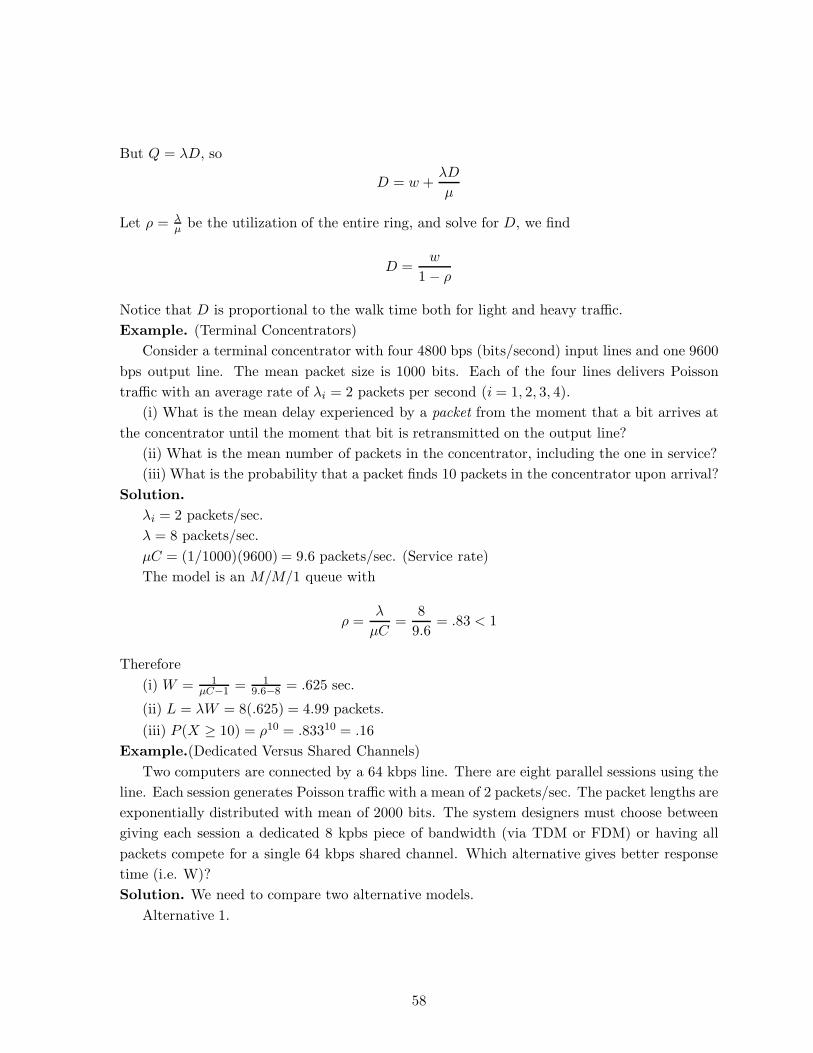
But Q = λD, so

D = w +λD

µ

Let ρ = λµ be the utilization of the entire ring, and solve for D, we find

D =w

1 − ρ

Notice that D is proportional to the walk time both for light and heavy traffic.

Example. (Terminal Concentrators)

Consider a terminal concentrator with four 4800 bps (bits/second) input lines and one 9600

bps output line. The mean packet size is 1000 bits. Each of the four lines delivers Poisson

traffic with an average rate of λi = 2 packets per second (i = 1, 2, 3, 4).

(i) What is the mean delay experienced by a packet from the moment that a bit arrives at

the concentrator until the moment that bit is retransmitted on the output line?

(ii) What is the mean number of packets in the concentrator, including the one in service?

(iii) What is the probability that a packet finds 10 packets in the concentrator upon arrival?

Solution.

λi = 2 packets/sec.

λ = 8 packets/sec.

µC = (1/1000)(9600) = 9.6 packets/sec. (Service rate)

The model is an M/M/1 queue with

ρ =λ

µC=

8

9.6= .83 < 1

Therefore

(i) W = 1µC−1 = 1

9.6−8 = .625 sec.

(ii) L = λW = 8(.625) = 4.99 packets.

(iii) P (X ≥ 10) = ρ10 = .83310 = .16

Example.(Dedicated Versus Shared Channels)

Two computers are connected by a 64 kbps line. There are eight parallel sessions using the

line. Each session generates Poisson traffic with a mean of 2 packets/sec. The packet lengths are

exponentially distributed with mean of 2000 bits. The system designers must choose between

giving each session a dedicated 8 kpbs piece of bandwidth (via TDM or FDM) or having all

packets compete for a single 64 kbps shared channel. Which alternative gives better response

time (i.e. W)?

Solution. We need to compare two alternative models.

Alternative 1.

58

For the TDM or FDM , each 8 kbps operates as an independent M/M/1 queue with λ = 2

packets/sec and µ = 4 packets/sec. Therefore

W =1

µ − λ=

1

4 − 2= 0.5 sec. = 500 msec.

Alternative 2.

The single 64 kbps is modeled as an M/M/1 queue with λ = 16 packets/sec and µ = 32

packets/sec. Therefore

W =1

µ − λ=

1

32 − 16= 0.0625 sec = 62.5 msec.

Splitting up a single channel into 4 fixed size pieces makes the response time worse. The

reason is that it frequently happens that several of the smaller channels are idle, while other

ones are processing work at the reduced

Exercise. Suppose that we have two M/M/1 models with parameters (λ1, µ1) and (λ2, µ2)

respectively. Show that if ρ1 = ρ2 and W1 = W2, then the two models are identical, (i.e. in

λ1 = λ2 and µ1 = µ2.)

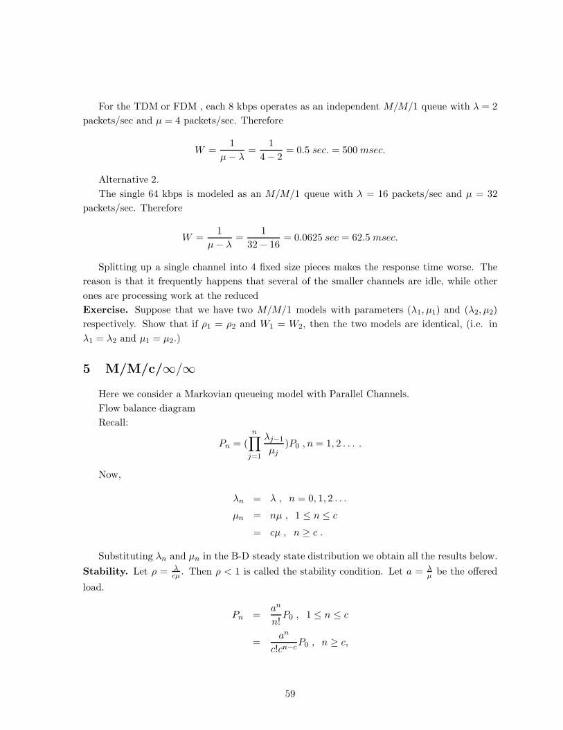
5 M/M/c/∞/∞Here we consider a Markovian queueing model with Parallel Channels.

Flow balance diagram

Recall:

Pn = (

n∏

j=1

λj−1

µj)P0 , n = 1, 2 . . . .

Now,

λn = λ , n = 0, 1, 2 . . .

µn = nµ , 1 ≤ n ≤ c

= cµ , n ≥ c .

Substituting λn and µn in the B-D steady state distribution we obtain all the results below.

Stability. Let ρ = λcµ . Then ρ < 1 is called the stability condition. Let a = λ

µ be the offered

load.

Pn =an

n!P0 , 1 ≤ n ≤ c

=an

c!cn−cP0 , n ≥ c,

59

where

P0 = [

c−1∑

n=0

an

n!+

∞∑

n=c

an

c!cn−c]−1

= [

c−1∑

n=0

an

n!+

ac

c!

∞∑

n=c

an−c

cn−c]−1

= [

c−1∑

n=0

an

n!+

ac

c!(1− ρ)]−1 .

Measures of Performance.

Lq :=

∞∑

n=c

(n − c)Pn =acρ

c!(1− ρ)2P0

Wq =Lq

λ= [

ac

c!(cµ)(1− ρ)2]P0

W = Wq +1

µ=

1

µ+ [

ac

c!(cµ)(1− ρ)2]P0

L = λW = Lq +λ

µ= a +

acρ

c!(1− ρ)2P0

U = ρ

Also the mean number of busy servers is given by

B = a =λ

µ.

FACT.

P (X ≥ c) =∞∑

n=c

Pn =ac

c!(1− ρ)P0 =

Pc

1 − ρ

=ac/c!

ac/c! + (1 − ρ)∑c−1

n=0 an/n!.

Remark. The relation P (X ≥ c) = Pc

1−ρ is called the Erlang second (delay) formula. It

represents the probability that customers would have to wait. (Or percentage of customers

that wait)

FACT. For an M/M/c − FCFS queue,

60

(i)

P (Tq = 0) =c−1∑

n=0

Pn = 1 − acp0

c!(1− ρ);

P (Tq > t) = (1− P (Tq = 0))e−cµ(1−ρ)t

=acp0

c!(1− ρ)e−cµ(1−ρ)t , t ≥ 0

(ii)

P (Tq > t|Tq > 0) = e−cµ(1−ρ)t , t > 0

(iii)

P (T > t) = e−µt[1 +ac(1− e−µt(c−1−a)

c!(1− ρ)(c− 1 − a)P0] , t ≥ 0

Proof. Let Wq(t) = P (Tq ≤ t)

Proof.

Wq(0) = P (Tq = 0) = P (X ≤ c− 1)

=

c−1∑

n=c

pn

= 1 −∞∑

n=0

pn

= 1 −∞

∑

n=c

an

c!cn−cp0

= 1 − ac

c!

∞∑

n=c

(a

c

)n−cp0

= 1 − ac

c!(1− p)p0

61

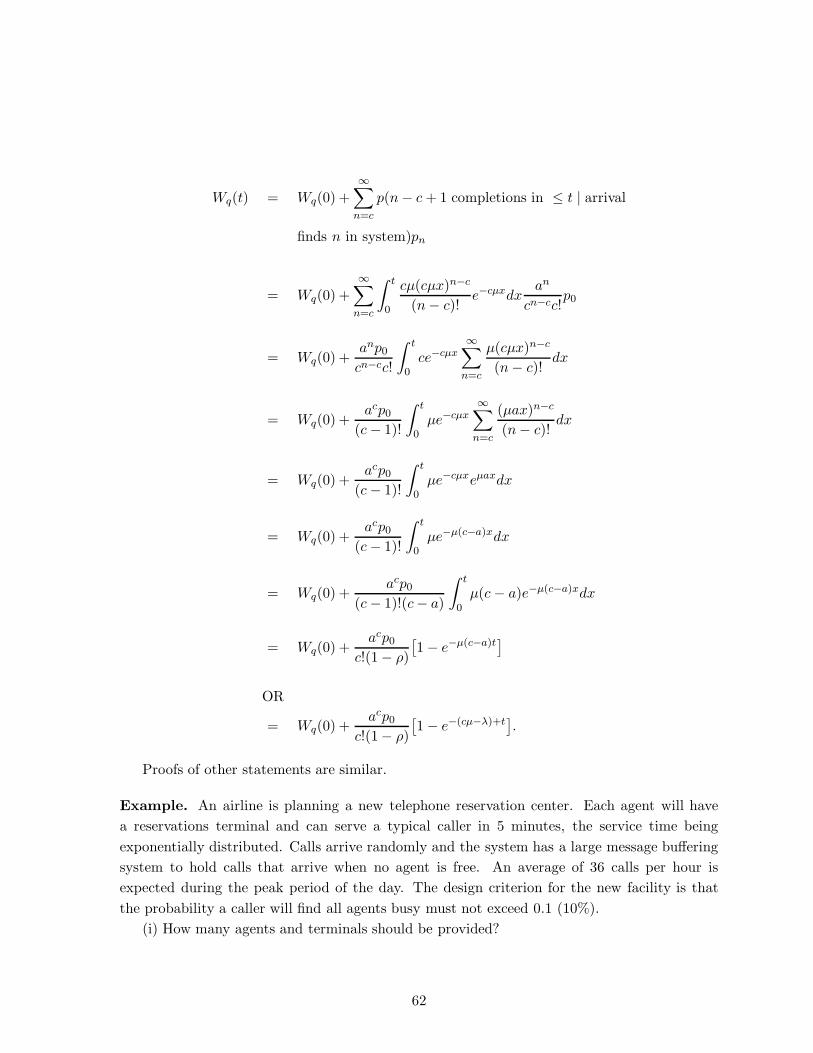
Wq(t) = Wq(0) +

∞∑

n=c

p(n − c + 1 completions in ≤ t | arrival

finds n in system)pn

= Wq(0) +

∞∑

n=c

∫ t

0

cµ(cµx)n−c

(n − c)!e−cµxdx

an

cn−cc!p0

= Wq(0) +anp0

cn−cc!

∫ t

0ce−cµx

∞∑

n=c

µ(cµx)n−c

(n − c)!dx

= Wq(0) +acp0

(c − 1)!

∫ t

0µe−cµx

∞∑

n=c

(µax)n−c

(n − c)!dx

= Wq(0) +acp0

(c − 1)!

∫ t

0µe−cµxeµaxdx

= Wq(0) +acp0

(c − 1)!

∫ t

0µe−µ(c−a)xdx

= Wq(0) +acp0

(c − 1)!(c− a)

∫ t

0

µ(c − a)e−µ(c−a)xdx

= Wq(0) +acp0

c!(1− ρ)

[

1 − e−µ(c−a)t]

OR

= Wq(0) +acp0

c!(1− ρ)

[

1 − e−(cµ−λ)+t]

.

Proofs of other statements are similar.

Example. An airline is planning a new telephone reservation center. Each agent will have

a reservations terminal and can serve a typical caller in 5 minutes, the service time being

exponentially distributed. Calls arrive randomly and the system has a large message buffering

system to hold calls that arrive when no agent is free. An average of 36 calls per hour is

expected during the peak period of the day. The design criterion for the new facility is that

the probability a caller will find all agents busy must not exceed 0.1 (10%).

(i) How many agents and terminals should be provided?

62

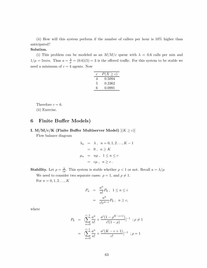
(ii) How will this system perform if the number of callers per hour is 10% higher than

anticipated?

Solution.

(i) This problem can be modeled as an M/M/c queue with λ = 0.6 calls per min and

1/µ = 5min. Thus a = λµ = (0.6)(5) = 3 is the offered traffic. For this system to be stable we

need a minimum of c = 4 agents. Now

c P (X ≥ c)

4 0.5094

5 0.23626 0.0991

Therefore c = 6.

(ii) Exercise.

6 Finite Buffer Models)

I. M/M/c/K (Finite Buffer Multiserver Model) [(K ≥ c)]

Flow balance diagram

λn = λ , n = 0, 1, 2 . . . , K − 1

= 0 , n ≥ K

µn = nµ , 1 ≤ n ≤ c

= cµ , n ≥ c .

Stability. Let ρ = λcµ . This system is stable whether ρ < 1 or not. Recall a = λ/µ

We need to consider two separate cases: ρ = 1, and ρ 6= 1.

For n = 0, 1, 2 . . . , K

Pn =an

n!P0 , 1 ≤ n ≤ c

=an

c!cn−cP0 , n ≥ c,

where

P0 = [

c−1∑

n=0

an

n!+

ac(1 − ρK−c+1)

c!(1− ρ)]−1 ; ρ 6= 1

= [

c−1∑

n=0

an

n!+

ac(K − c + 1)

c!]−1 ; ρ = 1

63

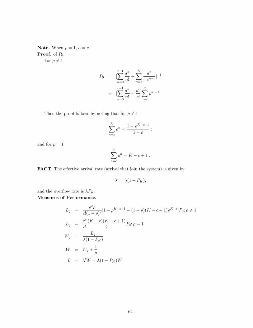
Note. When ρ = 1, a = c.

Proof. of P0.

For ρ 6= 1

P0 = [

c−1∑

n=0

an

n!+

K∑

n=c

an

c!cn−c]−1

= [

c−1∑

n=0

an

n!+

ac

c!

K∑

n=c

ρn]−1

Then the proof follows by noting that for ρ 6= 1

K∑

n=c

ρn =1 − ρK−c+1

1 − ρ;

and for ρ = 1K

∑

n=c

ρn = K − c + 1 .

FACT. The effective arrival rate (arrival that join the system) is given by

λ′ = λ(1− PK),

and the overflow rate is λPK .

Measures of Performance.

Lq =acρ

c!(1− ρ)2[1− ρK−c+1 − (1− ρ)(K − c + 1)ρK−c]P0; ρ 6= 1

Lq =cc

c!

(K − c)(K − c + 1)

2P0; ρ = 1

Wq =Lq

λ(1− PK)

W = Wq +1

µ

L = λ′W = λ(1− PK)W

64

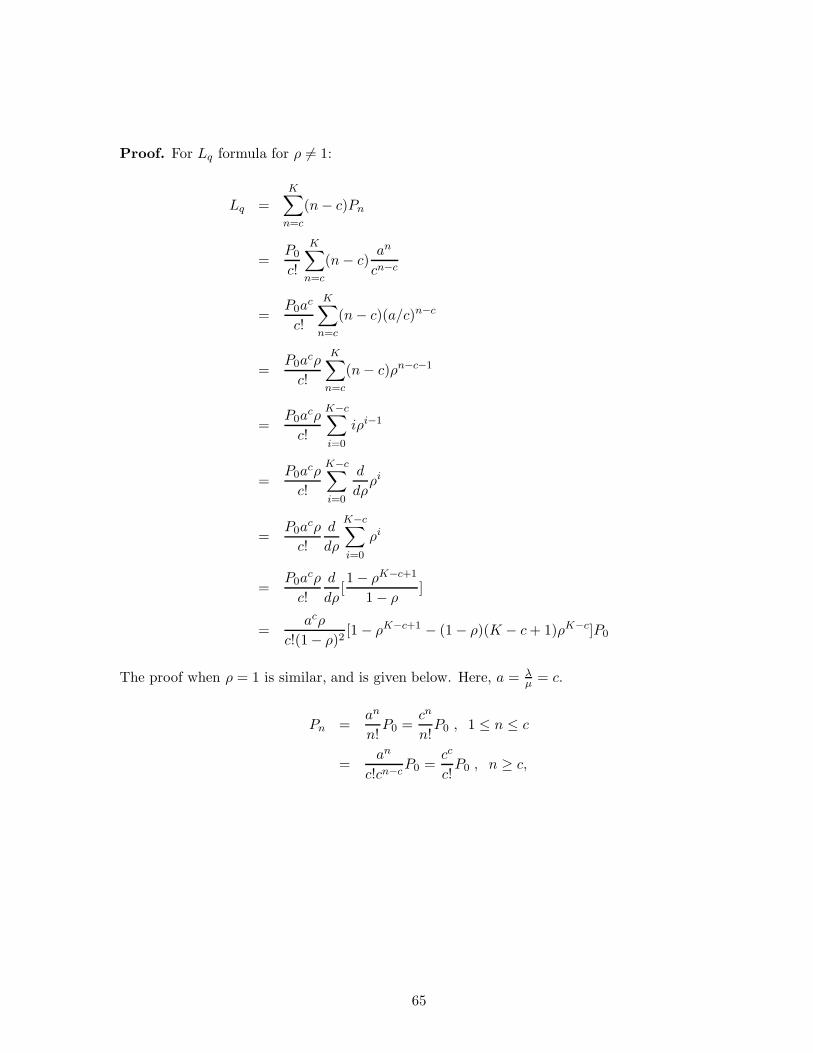
Proof. For Lq formula for ρ 6= 1:

Lq =

K∑

n=c

(n − c)Pn

=P0

c!

K∑

n=c

(n − c)an

cn−c

=P0a

c

c!

K∑

n=c

(n − c)(a/c)n−c

=P0a

cρ

c!

K∑

n=c

(n − c)ρn−c−1

=P0a

cρ

c!

K−c∑

i=0

iρi−1

=P0a

cρ

c!

K−c∑

i=0

d

dρρi

=P0a

cρ

c!

d

dρ

K−c∑

i=0

ρi

=P0a

cρ

c!

d

dρ[1 − ρK−c+1

1 − ρ]

=acρ

c!(1− ρ)2[1 − ρK−c+1 − (1 − ρ)(K − c + 1)ρK−c]P0

The proof when ρ = 1 is similar, and is given below. Here, a = λµ = c.

Pn =an

n!P0 =

cn

n!P0 , 1 ≤ n ≤ c

=an

c!cn−cP0 =

cc

c!P0 , n ≥ c,

65

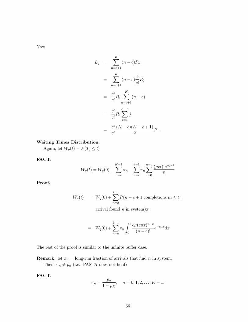
Now,

Lq =

K∑

n=c+1

(n − c)Pn

=

K∑

n=c+1

(n − c)cc

c!P0

=cc

c!P0

K∑

n=c+1

(n − c)

=cc

c!P0

K−c∑

j=1

j

=cc

c!

(K − c)(K − c + 1)

2P0 .

Waiting Times Distribution.

Again, let Wq(t) = P (Tq ≤ t)

FACT.

Wq(t) = Wq(0) +

K−1∑

n=c

πn −k−1∑

n=c

πn

n−c∑

i=0

(µct)ie−µct

i!

Proof.

Wq(t) = Wq(0) +

k−1∑

n=c

P (n − c + 1 completions in ≤ t |

arrival found n in system)πn

= Wq(0) +

k−1∑

n=c

πn

∫ t

0

cµ(cµx)n−c

(n − c)!e−cµxdx

The rest of the proof is similar to the infinite buffer case.

Remark. let πn = long-run fraction of arrivals that find n in system.

Then, πn 6= pn (i.e., PASTA does not hold)

FACT.

πn =pn

1 − pK, n = 0, 1, 2, . . . , K − 1.

66

Proof. For a birth/death process

λπj = λjpj (∗)

Now, sum over all j =⇒ λ =∑

λjpj

Therefore (*) =⇒ πj =λjpj

∑

λjpj

Recall

λj = λ, j ≤ k − 1

0, otherwise =⇒

πj =λpj

λ∑k−1

j=0 pj

=pj

1 − pK.

II. M/M/1/K (Finite Buffer Single Server Model)

Flow balance diagram

λn = λ , n = 0, 1, 2 . . . , K − 1

= 0 , n ≥ K

µn = µ , n = 1, 2 . . . , K.

Stability. Let ρ = λµ . This system is stable whether ρ < 1 or not.

We need to consider two separate cases: ρ = 1, and ρ 6= 1.

For n = 0, 1, 2 . . . , K, Pn = ρnP0. That is

Pn =ρn(1 − ρ)

1− ρK+1, ρ 6= 1

=1

K + 1, ρ = 1,

Remarks. (i) The stationary probabilities could be obtained directly from the stationary

probabilities of the M/M/1 model using truncation when ρ < 1. That is

Pn =ρn(1− ρ)∑K

n=0 ρn=

ρn(1 − ρ)

1 − ρK+1

(ii)

P0 =1 − ρ

1 − ρK+1, ρ 6= 1

=1

K + 1, ρ = 1,

67

FACT. The effective arrival rate (arrivals that join the system) is given by

λ′ = λ(1− PK) = µ(1− p0) .

In particular, if ρ 6= 1

λ′ =λ(1− ρK)

1 − ρK+1

and if ρ = 1

λ′ =λK

K + 1.

The rate at which customers are blocked (lost) is λPK.

Measures of Performance.

Case 1:ρ = 1 L = K/2

Case 2: ρ 6= 1

L :=

K∑

n=0

nPn =ρ

1− ρ− (K + 1)ρK+1

1 − ρK+1

U = 1 − P0 =λ′

µ=

ρ(1− ρK)

1 − ρK+1

Lq = L − (1 − P0) = L − λ′

µ= L − ρ(1− ρK)

1 − ρK+1

W =L

λ(1− PK)

Wq =Lq

λ(1− PK)

I = P0 =1 − ρ

1 − ρK+1

Example (Message Switching) Suppose the Co. has the same arrival pattern, message

length distribution, and line speed as described in the example. Suppose, however, that it

is desired to provide only a minimum number of message buffers required to guarantee that

PK < 0.005.

(i) How many buffers should be provided?

Solution. Need to find K such that

ρK(1− ρ)

1 − ρK+1= 0.005

where ρ = 0.88. Therefore K = 25.142607, i.e. K = 26. Thus we need 25 buffers.

68

(ii) For this number of buffers calculate L, Lq, W , and Wq.

Solution.

L = 6.44 messages

Lq = 5.573 messages

W = 1.62 seconds

Wq = 1.40 seconds

Exercise. Check these calculations using the formulas. Then compute λ0 := λpk, the overflow

rate.

7 M/M/c/c Erlang Loss Model

Flow balance diagram

For n = 0, 1, 2 . . . , c

Pn =an

n!P0 =

an/n!∑c

j=0 aj/j!.

Pc =ac/c!

∑cj=0 aj/j!

.

Remark.

B(c, a) = Pc, is called the Erlang loss probability

= P(all servers are busy)

= P(an arrival will be rejected)

= overflow probability

FACT. The effective arrival rate (arrivals that join the system) is given by λ′ = λ(1−Pc), and

the overflow rate is λPc.

Measures of Performance.

W =1

µ

L = λ′W = λ(1− Pc)/µ = a(1− Pc)

U = ρ(1 − Pc)

Note that Lq = Wq = 0 (why?).

69

Example. What is the minimal number of servers needed, in an M/M/c Erlang loss system,

to handle an offered load a = λ/µ = 2 erlangs, with a loss no higher than 2%?

Solution. Need to find c such that B(c, a = 2) ≤ 0.02.

B(0, 2) = 1

B(1, 2) = 2/3

B(2, 2) = 2/5

B(3, 2) = 4/19

B(4, 2) = 2/21 ≈ .095

B(5, 2) = 4/109 ≈ .037

B(6, 2) = 4/381 ≈ .01 < 0.02.

Therefore c = 6.

Applications. In many computer systems, there is a maximum number of connections that can

be established at any one time. Companies that subscribe to certain networks may only have a

certain number of virtual circuits open at any one instant, the number being determined when

the company subscribes to the service. ATM switches allow for a fixed number of outgoing

lines, so here too a fixed number of connections can coexist.

In all these and other cases, it is interesting to be able to compute the probability that

an attempt to establish a new connection fails because the maximum number of connections

already exists. We can model this environment by the Erlang loss model.

8 M/M/∞/∞ Unlimited Service Model

Flow balance diagram

For n = 0, 1, 2 . . . ,

Pn =ane−a

n!

Measures of Performance.

W =1

µ

L = λW =λ

µ

Note that Lq = Wq = 0 (why?).

Example. Calls in a telephone system arrive randomly at an exchange at the rate of 140 per

hour. If there is a very large number of lines available to handle the calls, that last an average

of 3 minutes,

70

(i) What is the average number of lines, L, in use? What is the standard deviation?

(ii) Estimate the 90th and 95th percentile of the number of lines in use.

Solution.

(i) This problem can be modeled as an M/M/∞ queue with λ = 140/60 arrivals per min

and 1/µ = 3min. Thus L = λµ = (14/6)(3) = 7

σ =√

L =√

7

(ii) Use the normal distribution as an estimate of percentile values.

90th percentile = 7 + 1.28√

7 = 10.38 or 10 lines.

95th percentile = 7 + 1.645√

7 = 11.35 or 11 lines.

9 Finite Population Models

I. M/M/1//N (Finite Population Single Server Model)(N ≥ 1)

Flow balance diagram

λn = (N − n)λ , n = 0, 1, 2 . . . , N

= 0 , n ≥ N

µn = µ , 1 ≤ n ≤ N .

Stability. This system is always stable. Recall a = λ/µ is called offered load per idle source.

For n = 0, 1, 2 . . . , N

Pn = [N !an

(N − n)!]P0 ,

where

P0 = [

N∑

n=0

N !an

(N − n)!]−1

Measures of Performance.

Lq :=

N∑

n=0

(n − 1)Pn = N − λ + µ

λ(1 − P0)

L :=

N∑

n=0

nPn = Lq + (1 − P0) = N − µ

λ(1− P0)

W =L

λ(N − L)=

N

µ(1 − p0)− 1

λ

Wq =Lq

λ(N − L)

71

FACT. The effective arrival rate (arrivals that join the system) is given by

λ′ =N

∑

n=0

λnPn = λ(N − L) = µ(1 − p0) .

Remarks. (i) Equating the effective arrival rate and effective departure rate gives

λ(N − L) = µ(1 − p0)

which leads to

L = N − µ

λ(1 − P0)

With this argument, the above formula is valid for non-exponential service times as well.

(ii) Note that W ≥ 1/u and W ≥ Nµ − 1

λ which is the case when p0 = 0. Thus we have the

following inequality

W ≥ max(N

µ− 1

λ,1

µ) .

Example. An OR analyst believes he can model the word processing and electronic mail

activities in his executive office as an M/M/1//4 queueing system. He generates so many

letters, memos, and email messages each day that four secretaries ceaselessly type away at their

workstations that are connected to a large computer system over an LAN . Each secretary works

on average, for 40 seconds before she makes a request for service to the computer system. A

request for service is processed in one second on average (processing times being exponentially

distributed). The analyst has measured the mean response time using his electronic watch (he

gets 1.05 seconds) and estimates the throughput as 350 requests per hour. The OR analyst

has decided to hire two additional secretaries to keep up with his productivity and will connect

their workstations to the same LAN if the M/M/1//6 model indicates a mean response time

of less than 1.5 seconds. Should he hire the two secretaries?

Solution.

First examine the current system. Here 1/λ = 40 sec/job, 1/µ = 1 sec/job.

With N = 4,

P0 = [

N∑

n=0

N !an

(N − n)!]−1 = 0.90253

L := N − µ

λ(1 − P0) = 4− 40(1− .90253) = .1012

λ′ = λ(N − L) = 0.09747 jobs/sec = 350.88 jobs/hr

W =L

λ′= 1.038

72

With N = 6, P0 = 0.85390, λ′ = 525.95 requests/hr and W = 1.069 seconds.

The OR analyst can add two workstations without seriously degrading the performance of

his office staff.

Exercise. Verify all calculations.

II. M/M/c//N (Finite Population Multiserver Model) (N ≥ c)

Flow balance diagram

λn = (N − n)λ , n = 0, 1, 2 . . . , N

= 0 , n ≥ N

µn = nµ , 1 ≤ n ≤ c

= cµ , n ≥ c .

Stability. This system is always stable. Recall a = λ/µ is the offered load per idle source.

For n = 0, 1, 2 . . . , N

Pn =N !an

(N − n)!n!P0 , 1 ≤ n ≤ c

=N !an

(N − n)!c!cn−cP0 , n ≥ c,

where

P0 = [

c−1∑

n=0

N !an

(N − n)!n!+

N∑

n=c

N !an

(N − n)!c!cn−c]−1

Measures of Performance.

L :=N

∑

n=0

nPn

λ′ = λ(N − L)

Lq = L − λ′

µ= (a + 1)L− aN

W =L

λ(N − L)

Wq =Lq

λ(N − L)

FACTS.

73

(i)The effective arrival rate (arrivals that join the system) is given by

λ′ =

N∑

n=0

λnPn = (N − L)λ

(ii) Arrival point (customer-average) probabilities are equal to the time-average probabilities

with one customer removed from the system. That is,

πn(N ) = pn(N − 1)

III. M/M/c/c/N (Finite Population Loss Model) (N ≥ c)

Flow balance diagram

λn = (N − n)λ , n = 0, 1, 2 . . . , c

= 0 , n ≥ c

µn = nµ , 1 ≤ n ≤ c

= 0 , n ≥ c .

Stability. This system is always stable. Recall a = λ/µ is the offered load per idle source.

For n = 0, 1, 2 . . . , c

Pn =N !an

(N − n)!n!P0 , 1 ≤ n ≤ c

=

(

Nn

)

an

∑ck=0

(

Nk

)

ak, 1 ≤ n ≤ c .

Note Pc is called Engest loss formula.

Remark. Let p = a1+a , i.e. a = p

1−p . Then an = pn

(1−p)n implies that for all n

an(1 − p)N = pn(1 − p)N−n

Now, multiplying the denominator and numerator of pn by (1 − p)N , we obtain

pn =

(

Nn

)

pn(1 − p)N−n

∑ck=0

(

Nk

)

pk(1 − p)N−k, 0 ≤ n ≤ c .

74

which is recognized as a truncated binomial probability distribution. Note also that if c = N ,

the distribution is binomial.

Measures of Performance.

L :=

c∑

n=0

nPn

λ′ = λ(N − L)

W =L

λ′

Lq = Wq = 0 .

FACTS. (i) πn(N ) = pn(N − 1) =(N−1

n )an

∑ck=0(

N−1

k )ak, for all values of n.

(ii) The stationary distribution pn is the same for non-exponential service times. (Insensi-

tivity)

10 System Availability

Consider a K-out-of-N system with repair.

- system functions if at least K components function

- i.e. system fails if N − K + 1 components fail

System states. 0, 1, . . . , N − K + 1, i.e. # of down components/machines

System Probabilities. p0, p1, . . . , pN−K+1

Objective. Compute system availiability, i.e.

P (system is available)

= long-run fraction of time the system is available

=

N−K∑

n=0

pn

= 1 − pN−K+1

Note.

pN−K+1 = unavailability of the system

= Prob.(system is unavailable)

Assumptions.

75

1. Time to failure is exp (λ)

2. Repair times are exp (µ).

3. # of servers, 1 ≤ c ≤ N − K + 1.

Notation. Let a =λ

µ

Flow Balance Diagram. (Birth-Death process)

Note. 1-out-of-N system (K = 1) is a usual finite population model.

Flow Balance Equations. (Global balance equations)

λ0p0 = µ1p1

λnpn + µnpn = λn−1pn−1 + µn+1pn+1, n = 1, 2, . . . , N − K + 1

where

λn = (N − n)λ, n = 0, 1, . . . , N − K + 1

µn = nµ n ≤ c

= cµ c ≤ n ≤ N − K + 1.

These equations lead to the detailed balance equations (DBE)

76

λnpn = µn+1pn+1 n = 0, 1, . . . , N − K

Solving the DBE, we get

p1 =Nλ

µp0 = Nap0

p2 =(N )(N − 1)

1 × 2a2p0

In general

pn =N !

(N − n)!n!anp0, 1 ≤ n ≤ c

pn =N !

(N − n)!c!cn−canp0, c ≤ n ≤ N − K + 1

p0 =

[

c−1∑

n=0

(

N

n

)

an +

N−K+1∑

n=c

N !

(N − n)!c!cn−1an

]−1

Remark. If each component has its own server, i.e. c = N − K + 1, then we get

pn =

(

N

n

)

an/

N−K+1∑

n=0

(

N

n

)

an, n = 0, 1, . . . , N − K + 1

In this case, the system is denoted by M/G//(

NK

)

, and probabilities pn are valid for any

service time distribution (insensitivity phenomenon).

Performance Measures.

− pN−K+1 =(N − K + 1)!

(K − 1)!c!cN−K+1−caN−K+1p0

is the unavailability of the system.

− System availability = 1 − pN−K+1 =

N−K∑

n=0

pn.

77

Exercise. Find the system availability when N = 5, λ = 3, µ = 5 and K = 3, K = 2, K = 1,

i.e. (3 systems, 3-out-of-5, 2-out-of-5, and 1-out-of-5).

11 Double Ended Queue

This model is also called synchronization queue, fork/join station, or kitting process.

Consider a queueing model consisting of two finite input buffers, B1 and B2, fed by arrivals

from two finite populations of sizes K1 and K2. The first population feeds the first buffer and

the second population feeds the second buffer. As soon as there is one part in each buffer, two

parts one from each buffer are joined and exit immediately. Therefore, at least one buffer has

no parts at all times and parts in the other buffer wait until one part is available in each buffer.

This model can be descibed by the well known taxi-cab problem where taxis and passengers

form two different queues, say the taxi queue and the passenger queue respectively. A passenger

(taxi) who arrives at the taxi stand without finding taxis(passengers) in the taxi (passenger)

queue has to wait in the passenger (taxi) queue and leaves as soon as a taxi (passenger) comes

to the stand. This model has many applications in various areas. Examples include paral-

lel processing, database concurrency control, flexible manufacturing systems, communication

protocols and so on.

Typically one is interestred in computing the mean number of jobs in each buffer, system

throughput, and characterization of the departure process, i.e. the distribution of time between

inter-departures.

Let the time until each member in population K1(K2) requests service i.e. joins the buffer is

exponential with parameter λ1(λ2). In this case the times between requests are exponential with

parameters niλi , where ni is the number of active elements in population (Ki−#inBi), i = 1, 2.

Note that a variation of this model is to consider two Poisson input processes and finite

buffers. It can be shown that the system with two Poisson input processes and infinite buffers

is unstable.

Model Analysis.

Let Xi(t) be the number of units in buffer Bi; i = 1, 2. Note that X(t) = X1(t)−X2(t) is a

birth-death process with state space S = −K2, . . . , 0, . . . , K1. The transition rates are given

by

q(i, i + 1) = K1λ1,−K2 ≤ i ≤ 0

= (K1 − i)λ1, 0 ≤ i ≤ K1 − 1

q(i, i− 1) = (K2 − i)λ2,−K2 + 1 ≤ i ≤ 0

= K2λ2, 0 ≤ i ≤ K1

78

Graph: State: −K2, . . . , K1.Now, we solve the birth death balance equations to compute pn, −K2 ≤ n ≤ K1.

Performance Measures.

Let L1 and L2 be the mean number of units in buffer B1 and B2 respectively. Moreover, let

λe be the effective arrival rate which is equal to the system throughput.

L1 =

K1∑

n=0

npn

L2 =

−1∑

n=−K2

−npn =

K2∑

n=1

np(−n)

λe =

K1∑

n=−K2

(q(n, n + 1) + q(n, n − 1))pn

Modified State Description.

In stead of above let X(t) = X1(t)−X2(t)+K2 which give a birth death process with state

space S = 0, . . . , K1 + K2. Using the birth death model, the transition rates are given by

λi = q(i, i + 1) and µi = q(i, i− 1), where

λn = K1λ1, 0 ≤ n ≤ K2

= (K2 + K1 − n)λ1, K2 ≤ n ≤ K2 + K1 − 1

µn = nλ2, 1 ≤ n ≤ K2

= K2λ2, K2 ≤ i ≤ K2 + K1 .

Remark. Because we have a finite stae process, this B/D process is stable. Recall that the

stationary distribution for any stable birth death process is given by

P0 =1

1 +∑∞

k=1

∏kj=1

λj−1

µj

(5.6)

Pn = (

n∏

j=1

λj−1

µj)P0 , n = 1, 2 . . . . (5.7)

Substituting λn and µn in the stationary equation formulas, we obtain

79

pn =Kn

1

n!(λ1

λ2)np0, 0 ≤ n ≤ K2

=KK2

1

∏ni=1(K2 + i)

K2!Kn−K2

2

(λ1

λ2)np0, K2 ≤ n ≤ K2 + K1

P0 = [

K2∑

n=0

n∏

j=1

Kj1

j!(λ1

λ2)n +

K2+K1+1∑

n=K2+1

KK2

1

∏ni=1(K2 + i)

K2!Kn−K2

2

(λ1

λ2)n]−1 (5.8)

Performance Measures with the Modified Model.

Let L1 and L2 be the mean number of units in buffer B1 and B2 respectively. Moreover, let

λe be the effective arrival rate which is equal to the system throughput.

L1 =

K2∑

n=0

(K2 − n)pn

L2 =

K1∑

n=0

np(K2 + n)

λe =

K2+K1∑

n=0

(λn + µn)pn

80

Chapter 6

System Reliability

Contents.

Reliability Theory

1 Introduction

Definition. Reliability, R(t), is usually defined as the probability that a device (system)

performs adequately over the interval [0, t].

Remark. R(t) means adequate performance over [0, t] not just at time t.

A system is a collection of components.

Examples: airplane, engines, brakes, etc.

Components can be independent or dependent (very complex).

Example: Automobile parts: wiring joints, brakes, transmission, exhaust, body, etc.

Structural function of a system.

Consider a system that is made up of n components (subsystems). Let the rv Xi represent

the performance of component i, i.e.

Xi = 1, if component i performs adequately during [0, t],

= 0, if component i fails during [0, t]

Let X be the performance of the system, i.e.

X = 1, if system performs adequately during [0, t],

= 0, if system fails during [0, t]

Remarks.

(i) X is called the structure function of the system.

(ii) One can think of X as the result of a random experiment. (e.g. toss n coins and let

X = 1 if at least k coins turn up heads, and 0 otherwise)

81

2 Types of Systems

Series Systems.

System fails if one component fails, equivalently, the system works iff all components work,

in which case

X = X1X2 . . .Xn = min(X1, . . .Xn)

Parallel Systems.

System functions if at least one component functions, equivalently, the system fails iff all

components fail. The structure function is given by

X = max(X1, . . .Xn) = 1 − (1 − X1)(1 − X2) . . . (1 − Xn)

k out of n Systems.

System works if at least k out of n components function properly. The system function is

given by

X = 1,n

∑

i=1

Xi ≥ k

= 0,

n∑

i=1

Xi < k

For a 2 out of 3 system, we have

X = X1X2X3 + X1X2(1− X3) + X1(1− X2)X3 + (1− X1)X2X3

Remark.

(i) A series system is k out of n system with k = n.

(ii) A parallel system is k out of n system with k = 1.

3 System Reliability

Consider a system made up of n mutually independent components. Let P (Xi = 1) = pi.

Note that E(Xi) = pi.

Definition. The system reliability r is defined as

r = P (X = 1) = E(X)

Series Systems.

82

The reliability of the system is given by

r = E(X) = E(X1X2 . . .Xn)

= E(X1)E(X2) . . .E(Xn)

= p1p2 . . . pn

Example. Suppose a system consists of n = 4 identical components linked in series. What

must be the value of p so that r = 0.95?

Solution. We have to solve the following equation

p4 = 0.95

which gives

p = 0.951/4 = 0.987 .

Parallel Systems.

The reliability of the system is given by

r = E(X) = E[1− (1− X1)(1 − X2) . . . (1 − Xn)]

= 1− E[(1− X1)(1− X2) . . . (1− Xn)]

= 1− (1− p1)(1 − p2) . . .(1 − pn)

If the system is homogeneous, then

r = 1 − (1 − p)n .

Example. Suppose p = 0.95. How many components must be linked in parallel so that the

system reliability r = 0.99?

Solution. We must have

0.99 = 1 − (1 − 0.95)n

that is

0.01 = 0.05n

Taking logarithms

n = ln0.01/ ln0.05 = 1.5372

So n = 2.

83

Example. Suppose a system consists of n = 3 components linked in parallel. What must be

the value of p so that r = 0.99?

Solution. We have to solve the following equation

1− (1− p)3 = 0.99

which gives

p = 1 − 0.011/3 = 0.7846 .

k out of n Systems.

For the 2 out of 3 system, we have

r = E[X ] = p1p2p3 + p1p2(1− p3) + p1(1 − p2)p3 + (1− p1)p2p3 .

More generally,

r = P (

n∑

i=1

Xi ≥ k)

Suppose all components are identical, i.e. p1 = p2 = . . . = pn. Then

r =

n∑

i=k

(n

i

)

pi(1− p)n−i

Example. Suppose a system consists of n = 8 iid components with p = 0.95. The system fails

if at least 4 components failed. What is the reliability of this system?

Solution.

r =

8∑

i=4

(

8

i

)

0.95i(0.05)8−i = 0.9999

Remark. For systems that are non of the above the system function can be represented as a

directed graph.

4 Reliability Using Failure Rates

Consider a single component. Let T be a rv that denotes the time to failure of the compo-

nent. Suppose T has a pdf f(t) and a df F (t) = P (T ≤ t).

The structure function X is then given by

X = 1, T ≥ t

= 0, T < t.

84

Therefore,

R(t) := P (X = 1) = P (T ≥ t) = 1 − F (t).

Hazard rate: Let the hazard rate (failure rate) be given by

h(t) =f(t)

1 − F (t)

Interpretation: h(t)dt is the probability that the system will fail in (t, t + dt) given that it

has survived until t.

Types of systems:

(i) systems with increasing failure rate (IFR)

(ii) systems with decreasing failure rate (DFR)

Remark. A system with exponential failure distribution is both IFR and DFR (why?)

FACT. Let T with df F (t) be the time to failure of a system. Then

R(t) := 1 − F (t) = e−∫ t

0h(u)du

Proof. Note that

h(t) =f(t)

1 − F (t)= − d

dtln(1− F (t))

That isd

dtln(1− F (t)) = −h(t)

That is

ln(R(t)) = −∫ t

0h(u)du

Thus

R(t) := 1 − F (t) = e−∫ t

0h(u)du

Corollary 4.1

f(t) = −dR(t)

dt= h(t)e−

∫ t

0h(u)du

(Called generalized exponential form)

Bounds for IFR Distributions.

FACTS.

(i) For exponential distributions

R(t) = e−λt

85

(ii) Lower bound:

R(t) ≥ e−λt, t < 1/λ

0, t ≥ 1/λ

(iii) Upper bound

R(t) ≤ 1, t ≤ 1/λ

e−wt, t > 1/λ,

where w is the solution of 1 − wλ = e−wt.

Having calculated (estimated) R(t) for each component, we use the results of previous

section to calculate the reliability of the whole system.

Sometimes we do not want to calculate a numerical value of reliability, but rather assess the

effect of different component designs on total (system) reliability.

FACTS.

(i) Series structures of independent IFR components (not necessarily identical) are also IFR.

(ii) Series structures of independent DFR components (not necessarily identical) are also

DFR.

(iii) K out of n systems of independent IFR identical components are also IFR.

(iv) Parallel structures of independent IFR identical components are also IFR.

Example. Find the failure rate and reliability for the Weibull df.

Solution. Recall the Weibull df.

F (t) = 1 − exp(−(t/α)β)

Now,

h(t) = λtβ−1

where λ is a constant given in terms of α and β.

Exercise.

Find the value of λ in terms of α and β.

R(t) = exp(−(t/α)β)

Mean life time =∫ ∞

0 tf(t)dt =∫ ∞

0 R(t)dt.

Example. An aircraft has four identical engines each of which has a failure rate λ. For a

successful flight at least two engines should be operating.

(i) What is the probability (reliability) that the aircraft will make a t hours successful flight?

Solution.

p = 1 − F (t) = e−∫ t

0λdu = e−λt

86

R(t) =

4∑

k=2

(

4

k

)

(e−λt)k(1 − e−λt)4−k

Simplify (exercise),

R(t) = 3e−4λt − 8e−3λt + 6e−2λt

(ii) What is the expected life-time, L, of the aircraft?

Solution.

E(L) =

∫ ∞

0

R(t)dt

=3

4λ− 8

3λ+

6

2λ

=13

12λ

Example. Suppose the aircraft is such that it needs at least one engine on each side for a

successful flight.

(i) Find new R(t).

Graph

Solution.

First, note that

X = [1 − (1 − X1)(1− X2)]2

EX = [1 − (1 − p)(1− p)]2 .

Therefore,

R(t) = [1 − (1 − e−λt)2]2

= [2e−λt − e−2λt]2

= e−4λt − 4e−3λt + 4e−2λt

(ii) Find the new expected life-time.

Solution.

exercise

Remark. For k out of n system with p = e−λt

R(t) =

n∑

i=k

(n

i

)

(e−λt)i(1− e−λt)n−i

87

Chapter 7

Appedix

Contents.

88

1 Final Project Guidelines

Abstract (one page)

1. Model description2. Results, findings

3. Significance

Project Details

1. Introduction2. Problem statement (show pictorially)

3. Sources of randomness, input data (distributions)4. Assumptions

5. Resulting model6. Objective, justification

7. Analysis (show all details)8. Validation and verification

9. Model results/Conclusions10. Sensitivity Analysis/ “What” if analysis11. Real Problem Conclusions

12. Recommendations13. Possible extensions

89