stochastic modelling of the spatial spread of influenza in germany

AUSTRIAN JOURNAL OF STATISTICS

Volume 35 (2006), Number 1, 5–20

Stochastic Modelling of the Spatial Spread of Influenza inGermany

Christiane Dargatz, Vera Georgescu, Leonhard HeldLudwig-Maximilians-University, Munich

Abstract: In geographical epidemiology, disease counts are typically avail-able in discrete spatial units and at discrete time-points. For example, surveil-lance data on infectious diseases usually consists of weekly counts of new in-fections in pre-defined geographical areas. Similarly, but on a different time-scale, cancer registries typically report yearly incidence or mortality countsin administrative regions.

A major methodological challenge lies in building realistic models for space-time interactions on discrete irregular spatial graphs. In this paper we willdiscuss an observation-driven approach, where past observed counts in neigh-boring areas enter directly as explanatory variables, in contrast to the parameter-driven approach through latent Gaussian Markov random fields (Rue andHeld, 2005) with spatio-temporal structure. The main focus will lie on thedemonstration of the spread of influenza in Germany, obtained through thedesign and simulation of a spatial extension of the classical SIR model (Huf-nagel et al., 2004).

Zusammenfassung: In der raumlichen Epidemiologie liegen Fallzahlen typ-ischerweise fur diskrete Gebiete und diskrete Zeitpunkte vor. Bei der Er-fassung infektioser Krankheiten beispielsweise zahlt man die wochentlichenInzidenzen in vorgegebenen Regionen. Ahnlich, aber auf einer anderen Zeit-skala, werden Krebsfalle jahrlich registriert.

Eine besondere Herausforderung liegt darin, eine Methode zur realistischenModellierung von raumlich-zeitlichen Zusammenhangen auf diskreten, un-regelmaßigen raumlichen Graphen zu entwickeln. In diesem Artikel beschafti-gen wir uns mit einem Ansatz, der bereits erfasste Falle in angrenzendenGebieten direkt als erklarende Variablen einbezieht, im Gegensatz zur Mod-ellierung durch latente Gauß-Markov-Zufallsfelder (Rue and Held, 2005) mitraumlich-zeitlicher Struktur. Dazu stellen wir die Ausbreitung von Influenzain Deutschland mittels einer raumlichen Erweiterung des klassichen SIR-Modells (Hufnagel et al., 2004) in Computersimulationen nach.

Keywords: Space-Time Interaction, Gaussian Markov Random Fields, Epi-demic Modelling, Stochastic Differential Equations, Global SIR Model, In-fluenza.

1 IntroductionThere has been much recent interest in space-time models for disease counts collectedin discrete spatial units and discrete time points. While most of the work has mainly fo-cused on non-infectious diseases, in particular on cancer, recently models for infectious

6 Austrian Journal of Statistics, Vol. 35 (2006), No. 1, 5–20

disease data have been developed. For non-infectious diseases, hierarchical Bayesian ap-proaches have been proposed, where latent parameters follow Gaussian Markov randomfield (GMRF) models (Waller et al., 1997, Knorr-Held and Besag, 1998, Knorr-Held,2000a, Lagazio et al., 2001, Lagazio et al., 2003, Schmid and Held, 2004). Common tothese models is the assumption that the observed counts are conditionally independent,given the latent parameters.

However, the allowance for realistic space-time interaction in GMRFs is non-trivial,one approach that dates back to Clayton (1996) is to use Kronecker product structures(see also Rue and Held, 2005, Section 3.4.3) for interaction parameters while keepingmain effects for overall spatial and temporal trends.

In this paper we will focus on a different modelling strategy, where past counts enterexplicitly in the disease rate and hence the conditional independence assumption is lost.This class of models, called observation-driven (Cox, 1981), is motivated by the fact thatparameter-driven models, such as the GMRF models mentioned above, are not able tocapture the epidemic trends observable in data on infectious diseases. Indeed, epidemicmodels have used such observation-driven models for decades; in particular the class ofSIR models (susceptible-infected-removed) has been extensively studied. However, thishas been done mainly in a purely temporal and simplistic context, ignoring the fact thatglobal epidemics spread in a spatio-temporal fashion.

A recent approach described in Hufnagel et al. (2004) fills this gap, proposing aspatio-temporal model on two scales (local and global) to describe the spread of the SARSepidemic based on stochastic differential equation models. Watts et al. (2005) developeda metapopulation model which incorporates mixing even at multiple scales. We adopt andextend the model of Hufnagel et al. (2004) and use it to investigate if it is able to describean influenza epidemic in Germany 2005.

A major requirement in SIR models is knowledge of the number of susceptibles. Insurveillance applications, often the whole population is considered as susceptible, dueto the lack of available data (e.g. Knorr-Held and Richardson, 2003). An alternativeapproach is to use a branching process model as an approximation to the SIR model. Thisclass of models has the advantage that it does not require knowledge of the number ofsusceptibles, however, some form of stationarity is needed to ensure that the stochasticprocess, describing the number of counts at each time point, does not explode to infinity.Held, Hohle, and Hofmann (2005) have used an extended version of this model in aseries of applications from surveillance data. In particular, they showed that maximumlikelihood estimation is straightforward and extended the model to the space-time domainusing a multivariate branching process formulation. However, the application of this classof model to highly infectious diseases such as influenza is perhaps not suitable, due to theunderlying assumption of stationarity.

In the next section, we will start with the classical SIR model and then describe theapproach by Hufnagel et al. (2004) to model the spatio-temporal spread of infectious dis-eases. In Section 3, we develop an algorithm for simulating this model. A central featureof the formulation is that the dispersal of infected cases in space is not necessarily solelylocal but also global, if necessary. For example, infected cases might travel through airtraffic large distances in a small amount of time. Based on data on air and train traffic inGermany, we define such a dispersal rate matrix for administrative regions in Germany

C. Dargatz et al. 7

and investigate whether simulations from such a model show similar patterns as an in-fluenza epidemic in Germany in 2005. Model parameters are chosen based on externalknowledge.

2 From the Standard Deterministic to a Global Stochas-tic SIR Model

2.1 Standard SIR ModelIn the SIR model, we divide a population into three categories: Those who are susceptibleto the disease (S), those who are infected and infectious (I), and those who are removedfrom the system because they are recovered and immune, or quarantined, or dead (R).With s, j, and r we denote the fractions of susceptible, infectious, and removed individu-als of the total population N . Transitions from one category to another happen accordingto

S + Iα−→ 2I , I

β−→ R ,

where α is the rate of an individual’s contacts per day which are sufficient to spread thedisease, and β−1 is the average infectious period. The infection dynamics in the standarddeterministic SIR model is given by the set of differential equations

ds/dt = −αsj , dj/dt = αsj − βj . (1)

Hence, while recovery follows a linear process, infections occur on high rate only whenboth the numbers of susceptibles and infectives are sufficiently large. Since we assumea closed population, i.e. ignoring births, non-related deaths, and migration during therelatively short duration of an influenza epidemic, we expect the size of the populationto be constant. The fraction of recovered individuals thus reads r = 1 − s − j. Theratio ρ = α/β is called the basic reproduction number and states a decisive parameter forthe course of the epidemic: When ρ−1 is greater than the initial fraction of susceptibles s0,no epidemic will develop. Otherwise, the epidemic will fall off as soon as the decreasingfunction s(t) drops below ρ−1.

In case of influenza, an infected individual acquires immunity to the strain he wasaffected by and can hence not become susceptible during the same wave of flu again.Therefore, there is no need for a transition from state R back to S. However, there aresteadily new antigen mutants of the influenza virus coming up, which is why at the begin-ning of the next epidemic the whole population will be susceptible again.

2.2 Stochastic SIR ModelBearing in mind that the infection and recovery processes are of rather stochastic thandeterministic character, we write (1) in terms of stochastic Langevin equations:

ds

dt= −αsj +

1√N

√αsj ξ1(t)

dj

dt= αsj − βj − 1√

N

√αsj ξ1(t) +

1√N

√βj ξ2(t),


where ξ1(t) and ξ2(t) are independent Gaussian white noise forces, modelling fluctuationsin transmission and recovery matters. These are of particular importance during the initialphase when the number of infected individuals is relatively small.

The above equations can be derived as a Gaussian approximation to the general stochas-tic epidemic model (see e.g. Daley and Gani, 1999, Section 3.3, and Andersson and Brit-ton, 2000, Section 5.5) in which the total population size tends to infinity.

2.3 Excursus: SLIR ModelIt is possible to also incorporate a latent status in our considerations, which yields thefollowing transitions, the so-called SLIR model:

S + Iα−→ L + I , L

ε−→ I , Iβ−→ R ,

where ε−1 is the average latent period. Let l denote the fraction of latent individuals ofthe total population. The differential equations then read

ds/dt = −αsj , dl/dt = αsj − εl , dj/dt = εl − βj

in the deterministic case and

ds

dt= −αsj +

1√N

√αsj ξ1(t)

dl

dt= αsj − εl − 1√

N

√αsj ξ1(t) +

1√N

√εl ξ3(t)

dj

dt= εl − βj − 1√

N

√εl ξ3(t) +

1√N

√βj ξ2(t)

in the stochastic model, where ξ3(t) accounts for noise in the duration of the latent period.Since our objective is the modelling of the spread of influenza, where an individual can

normally pass on the virus from the moment of infection, we from now on suppress theconsideration of latency. Nevertheless, the following observations can easily be adjustedto the SLIR model (cf. http://www.statistik.lmu.de/ dargatz/publications).

2.4 Global SIR ModelSo far, our model describes the spread of a disease in a single closed population under theassumption of homogeneous mixing. But this condition applies only as long as individualscover relatively short distances–an assumption that is not given in our fully connectedworld anymore, even if we restrict our focus to a comparatively small area like Germany.As suggested in Hufnagel et al. (2004), we introduce a network of subregions 1, . . . , n ofthe primarily observed area, each region i having a population size Ni being composed ofSi, Ii, and Ri susceptible, infectious and removed individuals. Whilst the local infectiondynamics within a subregion is given by the stochastic SIR model as introduced above,the global dispersal between the knots of the network is rated in a connectivity matrix γ =(γij)ij:

Si + Iiα−→ 2Ii , Ii

β−→ Ri , Siγij−→ Sj , Ii

γij−→ Ij .

C. Dargatz et al. 9

The system of stochastic differential equations now changes todsi

dt= −αsiji −

∑

k

γiksi +∑

k

γkisk +1√Ni

√αsiji ξ

(i)1 (t)

+1√Ni

√∑

k

γiksi ξ(i)4 (t)− 1√

Ni

√∑

k

γkisk ξ(i)5 (t)

dji

dt= αsiji − βji −

∑

k

γikji +∑

k

γkijk − 1√Ni

√αsiji ξ

(i)1 (t) +

1√Ni

√βji ξ

(i)2 (t)

+1√Ni

√∑

k

γikji ξ(i)4 (t)− 1√

Ni

√∑

k

γkijk ξ(i)5 (t) (2)

dri

dt= βji − 1√

Ni

√βji ξ

(i)2 (t).

for i = 1, . . . , n. Here, ξ1(t) = (ξ(1)1 (t), . . . , ξ

(n)1 (t)), ξ2(t), ξ4(t), and ξ5(t) are inde-

pendent vector-valued white noise forces which stand for fluctuations in transmission,recovery, and outbound and inbound traffic, respectively.

Since in the global model the single populations are not closed anymore due to mi-gration, the property si + ji + ri = 1, i = 1, . . . , n, does not necessarily hold. Instead,si, ji, and ri indicate the fractions of susceptible, infectious and removed individuals asmeasured by the original population Ni. That is why in (2) we also declared the formulafor ri.

3 Implementation

3.1 Keeping the System ClosedLet us focus on the Gaussian white noises ξj. The components of ξ1(t) and ξ2(t) (andalso of ξ3(t)) are all stochastically independent of each other, but we have to introducea weak form of dependence to the components of ξ4(t) and ξ5(t) due to the following:Since we assume the area of our n regions to be closed, we have to require

n∑i=1

(dsi

dt+

dji

dt+

dri

dt

)= 0 .

The left hand side of this equation reads

∑i

(−

∑

k

γiksi +∑

k

γkisk

)+

∑i

(−

∑

k

γikji +∑

k

γkijk

)(3)

+∑

i

1√Ni

√∑

k

γiksi +

√∑

k

γikji

ξ

(i)4 (t) (4)

+∑

i

1√Ni

√∑

k

γkisk +

√∑

k

γkijk

ξ

(i)5 (t) . (5)


Obviously, the two sums over i in (3) both equal 0. In order to also let rows (4) and (5)disappear, we correlate the components of ξ4(t) and those of ξ5(t) among each other suchthat equality with zero holds almost surely.

For the components of ξ4, we proceed as follows (see Knorr-Held, 2000b): Define

xi(t) :=1√Ni

√∑

k

γiksi(t) +

√∑

k

γikji(t)

.

We hence seekn∑

i=1

xi(t)ξ(i)4 (t) = 0 a.s. for all t. (6)

Define the n× n-matrices

M := In − 1

n1n1

′n =

n−1n− 1

n· · · − 1

n

− 1n

n−1n· · · − 1

n...

... . . . ...− 1

n− 1

n· · · n−1

n

,

where In ∈ Rn×n denotes the identity matrix and 1n = (1, . . . , 1)′ ∈ Rn×1. Furthermore,

Σ(t) := diag(x2

1(t), . . . , x2n(t)

)

and

Q(t) := MΣ(t)M =(qij(t)

)ij

with

qii =

(1

n2

∑

k 6=i

x2k(t) +

(n− 1

n

)2

x2i (t)

),

qij =

(1

n2

∑

k 6=i,j

x2k(t)−

n− 1

n2

(x2

i (t) + x2j(t)

))

for i 6= j,

and letu(t) :=

(x1(t)ξ

(1)4 (t), . . . , xn(t)ξ

(n)4 (t)

)′ ∼ N(0,Q(t)

), (7)

i.e. Q(t) is the covariance matrix of u(t). Then, as required,

var(xi(t)ξ

(i)4 (t)

)= qii(t) ≈ x2

i (t) for n large and i = 1, . . . , n

(xi(t) remains constant for t fixed, hence var(xi(t) ξ(i)4 (t))

!= x2

i (t)). Moreover,

E

(n∑

i=1

xi(t)ξ(i)4 (t)

)= 0 and var

(n∑

i=1

xi(t)ξ(i)4 (t)

)= 1′

nQ(t)1n = 0 ,

C. Dargatz et al. 11

yielding (6). Unfortunately, the desired property∑

i,j qij(t) = 0 yields the drawbackthat Q(t) is not positive definite and hence unsuitable as covariance matrix. Insteadof u(t), we hence consider a linear transformation Lu(t) with

L :=

(In−1 −1n−1

1′n−1 1

)∈ Rn×n ,

whose first n− 1 components have dispersion

P(t) := diag(x2

1(t), . . . , x2n−1(t)

)+ x2

n(t)1n−11′n−1 ∈ R(n−1)×(n−1) .

Draw π(t) = (π1(t), . . . , πn−1(t), 0)′ with

(π1(t), . . . , πn−1(t)

)′ ∼ N(0,P(t)

)

and retransform u(t) = (u1(t), . . . , un(t))′ = Mπ(t). We obtain

ξ(i)4 (t) =

ui(t)

xi(t), i = 1, . . . , n .

Note that, for any i, we have xi(t) > 0 as long as ri(t) < 1, since for all i ∈ {1, . . . , n}there is a k ∈ {1, . . . , n} with γik > 0 (i.e. each district is directly connected to at leastone other). However, if xi(t) = 0, the value of ξ

(i)4 (t) does not matter since in (4) it will

be multiplied by xi(t).Obtain ξ5 in the same way as ξ4, replacing xi(t) by

yi(t) :=1√Ni

√∑

k

γiksk(t) +

√∑

k

γikjk(t)

.

3.2 Numerical Scheme

Given initial conditions si(0), ji(0), and ri(0), i = 1, . . . , n, as well as fixed values forthe transmission rate α and the reciprocal average infectious period β, we simulate theepidemic process at discrete, equidistant instants in the time domain [0, tmax]. Definefunctions ap and bpk, p ∈ {s, j, r}, 1 ≤ k ≤ 5, such that the system of SDEs (2) becomes

dsi

(t)

dt= as

(t, si(t)

)+

5∑

k=1

bsk

(t, si(t)

)ξ

(i)k (t)

dji

(t)

dt= aj

(t, ji(t)

)+

5∑

k=1

bjk

(t, ji(t)

)ξ

(i)k (t) (8)

dri

(t)

dt= ar

(t, ri(t)

)+

5∑

k=1

brk

(t, ri(t)

)ξ

(i)k (t)


for i = 1, . . . , n. Let δ be the (suitably small) time step. For the approximation of thedifferential equations (8), we apply the Euler-Maruyama approximation scheme

si

(tm) = si

(tm−1

)+ as

(tm−1, si(tm−1)

)δ +

5∑

k=1

bsk

(tm−1, si(tm−1)

)4ξ(i)k (m)

√δ

ji

(tm) = ji

(tm−1

)+ aj

(tm−1, ji(tm−1)

)δ +

5∑

k=1

bjk

(tm−1, ji(tm−1)

)4ξ(i)k (m)

√δ (9)

ri

(tm) = ri

(tm−1

)+ ar

(tm−1, ri(tm−1)

)δ +

5∑

k=1

brk

(tm−1, ri(tm−1)

)4ξ(i)k (m)

√δ,

for m ≥ 1 and i = 1, . . . , n, where tm = mδ and 4ξ(i)k (m) = ξ

(i)k (tm) − ξ

(i)k (tm−1) (cf.

Kloeden and Platen, 1999).

3.3 Algorithm

After having fixed the parameters α, β, and γ, the time step δ and initial values for si,ji, and ri, i = 1, . . . , n, the proceeding for each instant of time now reads as follows(m = 0, . . . , btmax/δc − 1):

1. For i = 1, . . . , n, calculate

µi := α si(tm) ji(tm), νi := β ji(tm),

and

ηi :=n∑

k=1

γiksi(tm), ζi :=n∑

k=1

γkisk(tm), ρi :=n∑

k=1

γikji(tm), τi :=n∑

k=1

γkijk(tm).

2. For i = 1, . . . , n, compute xi = mi(√

ηi +√

ρi ) and yi = mi(√

ζi +√

τi ), wheremi :=

√Ni

−1.

3. Set P4 = diag(x2

1, . . . , x2n−1

)+ x2

n1n−11′n−1 and P5 = diag

(y2

1, . . . , y2n−1

)+

y2n1n−11

′n−1.

4. Generate π(j) =(π

(j)1 , . . . , π

(j)n

), j = 4, 5, with

(π

(j)1 , . . . , π

(j)n−1

) ∼ N(0,Pj)

and π(j)n = 0.

5. Compute u = (u1, . . . , un)′ = Mπ(4) and v = (v1, . . . , vn) = Mπ(5)with M =In − n−11n1

′n.

6. Evaluate ξ1, ξ2 ∼ N(0, In) and ξ4, ξ5 with ξ(i)4 = ui/xi, ξ

(i)5 = vi/yi, i = 1, . . . , n.

7. For i = 1, . . . , n, calculate


as(i) = −µi − ηi + ζi aj(i) = µi − νi − ρi + τi ar(i) = νi

bs1(i) = mi√

µi bj1(i) = −mi√

µi br1(i) = 0bs2(i) = 0 bj2(i) = mi

√νi br2(i) = −mi

√νi

bs3(i) = 0 bj3(i) = 0 br3(i) = 0bs4(i) = mi

√ηi bj4(i) = mi

√ρi br4(i) = 0

bs5(i) = −mi

√ζi bj5(i) = −mi

√τi br5(i) = 0.

8. Approximate si(tm+1), ji(tm+1), and ri(tm+1), i = 1, . . . , n, with Euler-Maruyamaformula (9).

9. For i = 1, . . . , n, correct approximation errors by setting negative values of si, ji,and ri equal to zero.

10. (Optional step.) Rescale si, ji, and ri, i = 1, . . . , n, via

si

(tm+1

) ← si

(tm+1

)(si

(tm+1

)+ ji

(tm+1

)+ ri

(tm+1

))−1

ji

(tm+1

) ← ji

(tm+1

)(si

(tm+1

)+ ji

(tm+1

)+ ri

(tm+1

))−1

ri

(tm+1

) ← ri

(tm+1

)(si

(tm+1

)+ ji

(tm+1

)+ ri

(tm+1

))−1.

With this transformation, we constantly adjust the fractions of susceptible, infected,and recovered individuals to the current population size of the respective region.

4 Initialization

We use our simulation program for the demonstration of spread of influenza in Germanyfor varying resolutions: for districts (”Landkreise/Stadtkreise”), counties (”Regierungs-bezirke”), and states (”Bundeslander”).

4.1 Dataset

The underlying data about incidences of influenza in Germany is taken from the RobertKoch Institute (RKI): SurvStat, http://www3.rki.de/SurvStat, deadline: 8 July 2005.We only consider cases categorized as A or A/B (i.e. no further differentiation), since itis the influenza A virus that is most responsible for national epidemics of the flu. Un-fortunately, the data suffers from underreporting. According to estimations of the Fed-eral Ministry of Health and Women, Austria (http://www.bmgf.gv.at), and the RobertKoch Institute (http://www.rki.de), the annual number of influenza cases is approx-imately 4.5% of the total population. However, only one out of 500 of these cases isreported to the RKI. Moreover, the number of announced cases depends on the numberof medical examinations induced and does hence not reflect the actual geographical dis-tribution. In particular, affections will be more clustered in the dataset than in reality.


4.2 Connectivity Matrix

The connectivity matrix γ describes the strength of traffic between the subunits of Ger-many. For its design we take into account the dispersal between adjacent regions, causede.g. by commuters, and the domestic train and air traffic. Each of these three componentsis provided with a weight regulating its influence.

At district level, we assume that the major part of the traffic between regions arisesfrom commuters. Data from the Federal Statistical Office (http://www.destatis.de/e home.htm) about the lengths of ways to work lead us to the assumption that about 30%of the employees work in a different district than their home town. Adding private traffic,we obtain an estimated fraction of 16% of the total population that is migrating betweendistricts every day, which is reflected by γ having an average row total of 0.16. We choosethe weights of the train and of the flight network to be 1/20 and 1/80 of the traffic betweenneighbored districts according to the annual amounts of travellers, which are about 200million in the inter urban rail services and 50 million in the domestic flight connections.Certainly, these weights depend on the kind of disease and time period under observation.For example, the influence of the flight network will be less when considering children’sdiseases, and during school terms an increasing national mixing rate should be considered.

Within the matrix γ, the strength of migration between two adjacent districts is mea-sured by their densities and numbers of surrounding districts. Our rail network modelconsists of 57 cities which are served by ICE trains. Data about flight connections wasobtained from the OAGflights database (http://www.oagflights.com) and composedas in Hufnagel et al. (2004).

For counties and states, we assume the migration between parts of Germany to bemore uniform than in the case of districts. For more details, see the supporting material.

4.3 Transmission Rate and Infectious Period

Before being able to run the simulation, we need an estimate of the parameters α and β.Recall that α is the daily number of contacts sufficient for infection an individual haswith other individuals, and β−1 is the average infectious period of the disease. Due tothese meanings, it is easy to estimate β, but more complicated to guess α. We hence tryto estimate the basic reproduction number ρ = α/β. For that, we return to the standarddeterministic SIR: Divide the second equation of (1) by the first one and obtain the time-independent differential equation

dj

ds= −1 +

1

ρs,

which has the explicit solution

j(t) = −s(t) +1

ρlog s(t) + c

with a constant c. At the very beginning of an influenza epidemic, almost all individuals ofthe considered population are susceptible, whilst the number of infected should be about


zero. With these assumptions, i.e. s0 = 1 and i0 = 0, we obtain c = 1. Consequently,

ρ =log s(t)

j(t) + s(t)− 1for all t ≥ 0. (10)

Certainly, the term on the right is not constant for the available data. Moreover, as timegoes by and safety measures like vaccination or isolation are increased, the reproductionnumber is going to fall. However, we assume ρ to be constant in time, but varying in space.From the application of formula (10) to our district-level data and limt→∞ s(t) = 0.955(compare Section 4.1) and limt→∞ j(t) = 0, we set

ρ(di) = 10−5di + 1.0179 ,

where di is the population density of region i. This relation reflects the intuitively clearfact that the disease is more likely to spread in areas with high population densities. Sincethe infectious period of influenza usually lasts for four to five days, we assume β = 2/9and calculate αi via βρ(di), i = 1, . . . , n.

5 Simulation ResultsIn this section we want to present the results of our simulations. We run the programfor different starting scenarios for both the deterministic and stochastic model and try theeffects of the parameters on the outcomes. Although we draw comparisons between the(highly under-)reported and the simulated data, we want to emphasize that the objectiveof this paper is neither to predict the future nor to exactly repeat former data, but to givean idea of the spatio-temporal spread of influenza and the effect of stochastic fluctuationson its outbreak.

Results of the simulations are returned as animated maps of Germany, which are avail-able at http://www.statistik.lmu.de/ dargatz/publications.

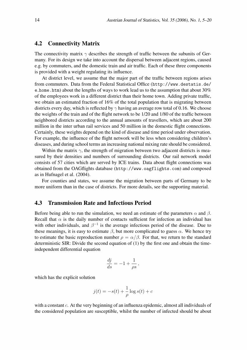
5.1 Long-Term SimulationsWe repeatedly run our simulation at district level with α and β as estimated in Section 4.3and with an initial number of infectious individuals according to week 5/2005 in ourdataset (Section 4.1). Though being probabilistic, the simulations generally yield the samepattern (see also Figure 1): From South Germany, where an increased level of prevalencewas observed in week 5, the disease bounces to Bremen and at the same time moves viaFrankfurt to North Rhine-Westphalia and Lower Saxony, from where it spreads to theEastern part of Germany and finally affects the whole nation. This shows surprisinglygood agreement with the actual course of the influenza epidemic in 2005 as demonstratedat http://influenza.rki.de. In the last graphic of Figure 1, we interpret the increasedmorbidity at the national borders, especially in North and East Germany, as edge effects.

As mentioned in Section 4.1, cases in our dataset appear more concentrated in oneregion than they probably are, which might be due to different reporting behavior. Incontrast to that, our simulation does not leave any district unaffected. The final size ofthe epidemic, which is the fraction of individuals that have been affected by the disease


0 0.02021129 0 0.02021129 0 0.02021129

0 0.02021129 0 0.02021129 0 0.02021129

Figure 1: Stochastic simulation of the spread of influenza in Germany. The initial situationcorresponds to week 5/2005 in the dataset. Displayed are the fractions of infectives atdays 50, 70, 85, 110, 133, and 150 after the starting point.

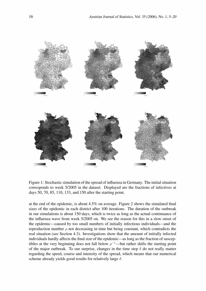
at the end of the epidemic, is about 4.5% on average. Figure 2 shows the simulated finalsizes of the epidemic in each district after 100 iterations. The duration of the outbreakin our simulations is about 150 days, which is twice as long as the actual continuance ofthe influenza wave from week 5/2005 on. We see the reason for this in a slow onset ofthe epidemic—caused by too small numbers of initially infectious individuals—and thereproduction number ρ not decreasing in time but being constant, which contradicts thereal situation (see Section 4.3). Investigations show that the amount of initially infectedindividuals hardly affects the final size of the epidemic—as long as the fraction of suscep-tibles at the very beginning does not fall below ρ−1—but rather shifts the starting pointof the major outbreak. To our surprise, changes in the time step δ do not really matterregarding the speed, course and intensity of the spread, which means that our numericalscheme already yields good results for relatively large δ.


Average final sizes of the epidemic in each region

districts

size

0.00

0.02

0.04

0.06

0.08

0.10

0.12

0.14

Figure 2: Average final sizes of the epidemic in the 438 German districts after 100 itera-tions, started at week 5/2005. The horizontal line indicates the mean of all bars.

5.2 One Week’s Forecasts

We initialize the computer program with data from various weeks of our dataset and sim-ulate the following week’s spread of the epidemic repeatedly. Figure 3 compares the dis-tributions of the proportions of infected individuals of the total population in week 7/2005for 2000 simulations of the stochastic model with the respective deterministic result andactual data for the three considered divisions of Germany and δ ∈ { 0.1, 1} (measuredin days). It turns out that the deterministic outcomes are similar for all resolutions andboth values of δ, but do not agree with the dataset, which is not surprising due to thehigh level of underreporting mentioned in Section 4.1. On county and state level, thestochastic results seem to be normally distributed with the deterministic value as mean,where the variance is smaller for δ = 0.1 than for δ = 1. In contrast to that, the prob-abilistic modelling on district level yields results that are larger than in the deterministiccase (for δ = 1 much more clearly than for δ = 0.1), though apparently also normallydistributed. We suspect the reason for this offset in the starting distribution of infectiousindividuals: While there are reported affections in almost all counties and states, preva-lences are concentrated on relatively few districts. When in our simulation the epidemicspreads to those districts with the initial fraction of infectives being zero, the stochasticfluctuations in this dynamics are kind of bounded to one side (compare with step 9 ofthe algorithm in Section 3). Obviously, this effect is deeper for larger values of δ. If wefocus on those few districts where morbidity was already present at the beginning of thesimulation, we obtain rather satisfying results already for δ = 1 (see Figure 4). For these


x

Den

sity

5.0 e−06 6.0 e−06 7.0 e−06 8.0 e−06 9.0 e−06 1.0 e−05 1.1 e−05

0 e

+00

2 e

+05

4 e

+05

6 e

+05

8 e

+05

x

Den

sity

5.0 e−06 6.0 e−06 7.0 e−06 8.0 e−06 9.0 e−06 1.0 e−05 1.1 e−05

0 e

+00

2 e

+05

4 e

+05

6 e

+05

8 e

+05

x

Den

sity

5.0 e−06 6.0 e−06 7.0 e−06 8.0 e−06 9.0 e−06 1.0 e−05 1.1 e−05

0 e

+00

1 e

+05

2 e

+05

3 e

+05

4 e

+05

5 e

+05

6 e

+05

x

Den

sity

5.0 e−06 6.0 e−06 7.0 e−06 8.0 e−06 9.0 e−06 1.0 e−05 1.1 e−05

050

0000

1000

000

1500

000

2000

000

2500

000

x

Den

sity

5.0 e−06 6.0 e−06 7.0 e−06 8.0 e−06 9.0 e−06 1.0 e−05 1.1 e−05

050

0000

1000

000

1500

000

2000

000

2500

000

x

Den

sity

5.0 e−06 6.0 e−06 7.0 e−06 8.0 e−06 9.0 e−06 1.0 e−05 1.1 e−05

050

0000

1000

000

1500

000

Figure 3: Distributions of the fractions of infectives after 2000 stochastic simulationsof one week’s spreads. The starting scenario corresponds to week 6/2005. The verticalmarks display the respective deterministic (bold line) and actual (thin line) outcomes ac-cording to the dataset. Simulations were performed on state, county, and district level(from the left to the right). The first row shows the results for δ = 1, the second onefor δ = 0.1.

x

Den

sity

0.0 e+00 5.0 e−06 1.0 e−05 1.5 e−05 2.0 e−05 2.5 e−05 3.0 e−05 3.5 e−05

0 e

+00

2 e

+04

4 e

+04

6 e

+04

8 e

+04

1 e

+05

x

Den

sity

0 e+00 1 e−05 2 e−05 3 e−05 4 e−05 5 e−05

010

000

2000

030

000

4000

050

000

x

Den

sity

0.00000 0.00005 0.00010 0.00015 0.00020 0.00025 0.00030

020

0040

0060

0080

0010

000

Figure 4: Distributions of the fractions of infectives in Berlin, Boblingen, and Bremer-haven (from the left to the right) after 2000 simulations with δ = 1. The starting sce-nario corresponds to week 6/2005. The vertical marks display the respective deterministic(thick line) and actual (thin line) outcomes.

districts, the actual data lies within the range of the stochastic results. We conclude thatthe stochastic simulation at district level is rather inappropriate as long as we considerrelatively short terms or cannot improve the quality of the underlying data.

6 Conclusion and Outlook

In this paper, we presented a global extension of the classical SIR model as well as techni-cal details for its implementation and initialization. Computer simulations provided quiterealistic demonstrations of the spread of diseases in Germany. The model assumes thatsome percentage of susceptibles and infectives of one region move to another region and


become part of the population in the other region. Since most trips considered here areday trips, a possible alternative model would be to keep the populations in each regionfixed and to assume that susceptibles and infectives have contacts between regions.

In future work, we will further refine the model both by considering this modificationand e.g. by involving time-dependent parameters (cf. Sections 4.3 and 5.1). Furthermore,we intend to deal with the question of finding surveillance strategies in case of a suddenoutbreak of an epidemic, like specific isolation, vaccination or observation of migration.One main purpose of our research will certainly involve the application of more formalstatistical inference techniques for estimating the model parameters based on availabledata from surveillance databases.

Acknowledgements

The authors are grateful to an unknown referee for insightful and encouraging comments.

References

Anderson, R., and May, R. (1991). Infectious Diseases of Humans. Oxford: OxfordUniversity Press.

Andersson, H., and Britton, T. (2000). Stochastic Epidemic Models and Their StatisticalAnalysis (Vol. 151). New York: Springer.

Clayton, D. (1996). Generalized linear mixed models. In W. Gilks, S. Richardson,and D. Spiegelhalter (Eds.), Markov Chain Monte Carlo in Practice (p. 275-301).London: Chapman & Hall.

Cox, D. (1981). Statistical analysis of time series. Some recent developments. Scandina-vian Journal of Statistics, 8, 93-115.

Daley, D., and Gani, J. (1999). Epidemic Modelling: An Introduction (Vol. 15). Cam-bridge: Cambridge University Press.

Held, L., Hohle, M., and Hofmann, M. (2005). A statistical framework for the analysis ofmultivariate infectious disease surveillance counts. Statistical Modelling, 5, 187-199.

Hufnagel, L., Brockmann, D., and Geisel, T. (2004). Forecast and control of epidemics ina globalized world. Proceedings of the National Academy of Sciences, 101, 15124-15129.

Kloeden, P., and Platen, E. (1999). Numerical Solution of Stochastic Differential Equa-tions (3rd ed.). Berlin, Heidelberg, New York: Springer.

Knorr-Held, L. (2000a). Bayesian modelling of inseperable space-time variation in dis-ease risk. Statistics in Medicine, 19, 2555-2567.

Knorr-Held, L. (2000b). Dynamic rating of sports teams. Journal of the Royal StatisticalSociety, Series D (The Statistician), 49, 261-276.

Knorr-Held, L., and Besag, J. (1998). Modelling risk from a disease in time and space.Statistics in Medicine, 17, 2045-2060.

Knorr-Held, L., and Richardson, S. (2003). A hierarchical model for space-time surveil-lance data on meningococcal disease incidence. Applied Statistics, 52, 169-183.


Lagazio, C., Biggeri, A., and Dreassi, E. (2003). Age-period-cohort models and diseasemapping. Environmetrics, 14, 475-490.

Lagazio, C., Dreassi, E., and Biggeri, A. (2001). A hierarchical Bayesian model forspace-time variation of disease risk. Statistical Modelling, 1, 17-29.

Rue, H., and Held, L. (2005). Gaussian Markov Random Fields: Theory and Applications(Vol. 104). London: Chapman & Hall.

Schmid, V., and Held, L. (2004). Bayesian extrapolation of space-time trends in cancerregistry data. Biometrics, 60, 1034-1042.

Waller, L., Carlin, B., Xia, H., and Gelfand, A. (1997). Hierarchical spatio-temporalmapping of disease rates. Journal of the American Statistical Association, 92, 607-617.

Watts, D., Muhamad, R., Medina, D., and Dodds, P. (2005). Multiscale, resurgentepidemics in a hierarchical metapopulation model. Proceedings of the NationalAcademy of Sciences, 102, 11157-11162.

Author’s addresses:

Christiane DargatzDepartment of StatisticsLudwig-Maximilians-University MunichLudwigstraße 3380539 MunichGermanyTel: +49 89 2180-2232Fax: +49 89 2180-5040E-mail: [email protected]: http://www.stat.uni-muenchen.de/ dargatz/index en.html

Vera GeorgescuE-mail: [email protected]

Leonhard HeldDepartment of StatisticsLudwig-Maximilians-University MunichLudwigstraße 3380539 MunichGermanyTel: +49 89 2180-6407Fax: +49 89 2180-5040E-mail: [email protected]: http://www.stat.uni-muenchen.de/ leo/index e.html

stochastic modelling of the spatial spread of influenza in germany

Documents