stochastic solvency testing in life insurance · stochastic solvency testing methods have existed...
TRANSCRIPT

Stochastic Solvency Testing in Life Insurance
Prepared by Genevieve Hayes
Presented to the Institute of Actuaries of Australia 2009 Biennial Convention, 19-22 April 2009
Sydney, New South Wales
This paper has been prepared for the Institute of Actuaries of Australia’s (Institute) 2009 Biennial Convention The Institute Council wishes it to be understood that opinions put forward herein are not necessarily those of the Institute and
the Council is not responsible for those opinions.
© Genevieve Hayes 2009
The Institute will ensure that all reproductions of the paper acknowledge the Author/s as the author/s, and include the above copyright statement:
The Institute of Actuaries of Australia Level 7 Challis House 4 Martin Place
Sydney NSW Australia 2000 Telephone: +61 2 9233 3466 Facsimile: +61 2 9233 3446
Email: [email protected] Website: www.actuaries.asn.au

Stochastic Solvency Testing in Life Insurance
1
Stochastic Solvency Testing in Life Insurance
Genevieve Hayes
Abstract
Stochastic solvency testing methods have existed for more than 20 years, yet there has been little research conducted in this area, particularly in Australia. This is for a number of reasons, the most pertinent of which being the lack of computing capabilities available in the past to implement more sophisticated techniques. However, recent advances in computing have made stochastic solvency testing possible in practice and have resulted in a trend towards this being done in advanced studies. The purpose of this paper is to present a realistic solvency testing model that could potentially be used by Australian Life Insurers. The model has been developed in anticipation that the Australian insurance regulator, APRA, will ultimately follow the world trend, requiring stochastic solvency testing to be carried out in Australia; and is constructed from three interconnected stochastic sub-models used to describe the economic environment and the mortality and lapsation experience of the portfolio of policies under consideration: (i) a modified CAS/SOA economic sub-model; (ii) either a Poisson or negative binomial (NB1) distribution (depending on the policy type considered) as the mortality sub-model; and (iii) a normal-Poisson lapsation sub-model. Based on tests carried out using this model, it is demonstrated that, for portfolios of level and yearly-renewable term insurance business, the current deterministic solvency capital requirements provide little protection against insolvency. Key words: stochastic; solvency testing; life insurance; mortality; lapsation; asset models; capital; value at risk; simulation.
1 Introduction One of the most important goals of any business is to remain solvent, as it can no longer continue its operations if it becomes insolvent, except in special circumstances where the government bails out the company by injecting capital. In the case of financial services institutions, such as banks and insurance companies, continued solvency is of importance, not just to the institution, but also to account/policyholders who could potentially face economic hardship if such an institution were to collapse. The 2001 collapse of Australian General Insurer HIH Insurance illustrates the adverse consequences to the public of such an event. As a result, the financial services industry is one of the most highly regulated industries, and all advanced economies have in place legislation designed to minimise the risk of a financial services institution going bankrupt. The legislation generally requires such institutions to hold capital greater than a specified minimum amount, often referred to as the solvency capital requirement, at all points in time. This paper focuses on the calculation of this quantity in the context of the Australian Life Insurance industry. Currently, Australian Life Insurers are required to calculate their solvency capital requirements on a deterministic basis using formulae set out in Life Insurance Prudential Standards LPS2.04 and LPS3.04. However, recently there has been a trend in advanced economies, such as Switzerland and the European Union countries, towards calculating insurer solvency capital requirements using stochastic techniques, thereby requiring insurers

Stochastic Solvency Testing in Life Insurance
2
to hold a capital amount that satisfies a probability-based criterion. For example, insurers might be required to hold an amount of capital sufficiently large so that there is a 99.5% chance that, in one year's time, the insurer's assets will exceed its liabilities. In order to satisfy such a criterion, the insurer must attempt to determine the probability distributions of the values of its assets and liabilities, or sometimes just of its capital holdings, at future points in time. These distributions usually need to be determined using computer-intensive simulation techniques. It was due to the unavailability of inexpensive, high-speed computers in the past that deterministic solvency testing techniques were used almost exclusively in all countries, and it is because of the easier access to such computers in recent years that stochastic solvency testing techniques have suddenly come to prominence. It is possible that, in keeping with this trend, the Australian insurance regulator, APRA, will ultimately require Australian Life Insurers to calculate their solvency capital requirements using stochastic methods. Such being the case, there is a need to develop a realistic asset-liability model that can be used for this purpose. In this paper, such a model is presented and the model is then used to assess whether the current Australian deterministic solvency capital criteria are appropriate, based on four commonly used stochastic solvency criteria: the 99.5% Value at Risk (VaR) and Tail Value at Risk (TVaR) of the change in capital distribution over a one year time horizon, and the 95% VaR and TVaR of the change in capital distribution over a three year time horizon. The presented model is a simulation model comprising three interconnected stochastic sub-models used to describe the economic environment and the mortality and lapsation experience. It is demonstrated, using Australian economic and Life Insurance data, that the “best” sub-model in each case (out of the range of models under consideration) is a modified CAS/SOA1 economic sub-model, a Poisson or negative binomial (depending on the policy type considered) mortality sub-model, and a normal-Poisson lapsation sub-model. Tests conducted in this paper demonstrate that, although the current deterministic requirements are sufficiently high for portfolios of investment-linked or “traditional” (endowment insurance) policies, they provide very little protection against insolvency for portfolios of “traditional” term insurance or for portfolios of “modern” yearly-renewable term insurance under some of the solvency criteria. Sensitivity tests conducted in association with these investigations show that the (stochastic) total asset requirements calculated using the solvency testing model are virtually unaffected by ignoring the over-dispersion that was found to be present in the mortality and lapsation data used in this paper, or dependency relationships that were found to exist between the economy and mortality rates, and the economy and lapsation rates. However, for some policy types, the requirements are significantly affected by changing the sub-model used to forecast the economic variables, or simplifying the formulae used to determine the mean mortality and lapsation rates in the sub-models used to forecast future mortality and lapsation experience. The implication of this latter result is that, if APRA is to require Life Insurers to calculate their solvency capital requirements using stochastic methods, then, in order to ensure consistency between insurers, some guidance should be provided with regard to the nature of the solvency testing model used. The structure of this paper is as follows: Section 2 provides an overview of what is meant by stochastic solvency testing, as well as providing a review of the current solvency legislation in place in Australia and in several other countries throughout the world. In Section 3, the main data sets used in this paper are described. The stochastic solvency testing model used in this paper is described in Section 4 and the method of implementation of the model is set out in Section 5. Section 6 summarises the results of comparing the solvency capital requirements calculated using the stochastic solvency model with those calculated under LPS2.04 and LPS3.04, and provides a sensitivity analysis of these results; and Section 7 concludes this paper by discussing its limitations and suggesting possibilities for future research.
1 Casualty Actuarial Society/Society of Actuaries

Stochastic Solvency Testing in Life Insurance
3
2 Life Insurance Solvency Testing: A Review
2.1 Stochastic Solvency Testing In the context of accounting, a business is considered to be solvent if it can pay its debts as they fall due. Thus, a business is generally considered to be solvent if its assets exceed its liabilities. The difference between assets and liabilities is referred to as capital. In the context of insurance, however, the values of the insurer’s assets and liabilities are uncertain (that is, they are stochastic quantities) and this uncertainty should be allowed for in any insurer solvency calculations. In spite of this, traditionally an insurer's solvency position has been evaluated using prescribed formulae that ignore the random nature of these amounts, that is, on a deterministic basis. An insurer was considered to be solvent if, at the valuation date, its assets were greater in value than its liabilities (both policy liabilities and non-policy liabilities), with policy liabilities valued using deterministic techniques and conservative valuation assumptions enforced so as to include an implicit risk margin in the estimate (more recently, an explicit deterministic risk margin was added to the best estimate of the policy liabilities instead of an implicit margin). Deterministic methods were used to evaluate solvency primarily due to the lack of computational capabilities required to implement more advanced techniques. However, stochastic asset and liability valuation techniques have existed for the past 25 years and in recent years, due to advances in computing, there has been a trend towards stochastic solvency testing. Stochastic solvency testing involves determining probability distributions for the insurer’s assets at time t and liabilities at time t, denoted A(t) and L(t) respectively, or sometimes, just for the insurer's capital at time t, C(t), where C(t) = A(t) – L(t) and using these to determine the amount of capital the insurer must hold at the solvency testing date such that a probability-based solvency criterion is satisfied. An insurer is then considered to be solvent if the amount of capital that it is currently holding is greater than this amount. Two commonly used probability-based solvency criterion or risk measures are the Value at Risk (VaR) and Tail Value at Risk (TVaR). The VaR risk measure is commonly used in banking and referred to in Basel II (BIS (2006)), the second Basel Accord produced by the Bank for International Settlements (BIS), which makes recommendations for bank capital regulations. The 100(1 - α)% VaR of an insurer’s capital distribution is defined as the minimum amount of capital that the insurer must hold at the solvency testing date so that the probability that the insurer’s capital holdings at some future point or points in time will be greater than 0 is greater than or equal to 100(1 - α)%, where 0 < α < 1 and α is specified in advance, often in the legislation of the country that the insurer operates in. The TVaR risk measure is an extension of the VaR. The 100(1 - α)% TVaR of an insurer’s capital distribution is equal to the expected shortfall in capital given that one of the worst 100(1 - α)% of scenarios has occurred. That is, the expected shortfall of capital given that the 100(1 - α)% VaR capital requirement is insufficient to ensure solvency at the specified future point or points in time. The TVaR capital requirement will always be greater than the VaR capital requirement (for the same value of α). Additional risk margins may also be added to this minimum capital amount, as in the deterministic case. Specifically, risk margins are also often added to allow for “the hypothetical cost of regulatory capital necessary to run off all the insurance liabilities, following financial distress of the company” (Sandström (2006, p.149)). These are referred to as Cost of Capital risk margins and are included so as to provide adequate risk compensation for a hypothetical insurer who may take over the portfolio in the future. CEA (2006) and FOPI (2006) give methodologies for calculating such risk margins.

Stochastic Solvency Testing in Life Insurance
4
2.2 Solvency Legislation In Australia, three actuarial standards exist that set out the statutory requirements for the valuation of policy liabilities for realistic profit reporting, solvency and capital adequacy purposes. These standards were made by the Life Insurance Actuarial Standards Board (LIASB), and reissued by the Australian Prudential Regulatory Authority (APRA) in 2008. All Life Insurers with operations in Australia are obligated to comply with these standards. LPS1.04 requires the realistic valuation of the life policies of the insurer, providing for the emergence of profit from life policies as it is earned, while LPS2.04 and LPS3.04 require the determination of policy liabilities using prescribed assumptions that are more conservative than best estimate assumptions and also outline the statutory capital requirements for Australian Life Insurers. The amounts calculated under LPS2.04 and LPS3.04, the solvency requirement and capital adequacy (cap. ad.) requirement, respectively, are the amounts the insurer must hold so as to be considered, by APRA, to be solvent in the short term (in the case of the solvency requirement) and likely to remain solvent in the long term (in the case of the capital adequacy requirement). By definition, the capital adequacy requirement is always at least as great as the solvency requirement, and for regulatory purposes an insurer must hold assets greater than its capital adequacy requirement, although it is not considered to be insolvent for statutory purposes unless its assets fall below its solvency requirement. If an insurer’s assets fall below its capital adequacy requirement, this serves as an early warning signal to APRA, allowing it the opportunity to intervene in order to prevent the insurer from becoming insolvent, if at all possible. The difference between the insurer's solvency requirement and its best estimate liabilities (both policy and non-policy liabilities) can be thought of as its solvency capital requirement, with the insurer's capital adequacy capital requirement similarly defined. No requirement is made for the actuary to use stochastic assumptions under any of these three standards, and in practice, most actuaries use deterministic assumptions. Since the solvency and capital adequacy requirements are calculated deterministically, the probabilities of adequacy of these requirements are unknown, as is whether these probabilities are consistent between different policy types and between different insurers, although according to Karp (2002), “the capital adequacy risk criterion was set at a 2% probability of assets falling below the required solvency level at the next annual balance date” and “the solvency risk criterion was set at a 5% probability of assets falling below liabilities within any of the next three annual balance dates” (p. 5). To determine whether this is true, it is necessary to use stochastic solvency testing methods. Stochastic reserving methods are currently mandated in Australia for General Insurers under APRA Prudential Standard GPS 310. Under this standard, the insurer must hold a risk margin above the central estimate of the value of its liabilities such that the liabilities are valued at the 75% level of sufficiency (or at the central estimate plus one half of the coefficient of variation, if this amount is greater than the 75% level of sufficiency). In addition, the insurer must hold capital greater than its minimum capital requirement, as specified under APRA Prudential Standard GPS 110. The insurer's minimum capital requirement may be calculated using a prescribed (deterministic) method or the insurer may develop its own internal capital measurement model and use that to calculate its minimum capital requirement (subject to APRA's approval of the model). If the internal model based approach is used, the insurer must hold sufficient capital such that the insurer's probability of default over a one year time horizon is reduced to 0.5% or below. In 2004, the International Actuarial Association (IAA) published a report (IAA (2004)) making recommendations on insurer solvency assessment. Three recommendations of this report (p. 5) were:
• “A reasonable period for the solvency assessment time horizon, for purposes of determining an insurer's current financial position is about one year;”
• “The amount of required capital must be sufficient with a high level of confidence, such as 99%, to meet all obligations for the time horizon as well as the present value

Stochastic Solvency Testing in Life Insurance
5
• The most appropriate risk measure for solvency assessment is the Tail Value at Risk as it requires insurers to hold an additional capital amount, above the Value at Risk capital amount, which is greater for insurers with more positively skewed loss distributions (that is, insurers who are more likely to experience catastrophic losses, must hold a greater amount of capital).
Some major countries are already in the process of introducing the requirement of stochastic solvency testing into their Life Insurance legislation. The European Commission is currently in the process of reviewing the existing European Union (EU) solvency regime (Solvency I) with the objective of establishing “a solvency system that is better matched to the true risks of an insurance company” (CEA and Mercer Oliver Wyman (2005, p.1)). This new system is referred to as Solvency II and it is anticipated that it will come into effect in the EU member states by the end of 2010. At the time of writing this, the requirements of Solvency II have yet to be finalised. However, a recent press release issued by the European Union (EU (2007)) stated that under Solvency II “insurers must have available resources sufficient to cover a Solvency Capital Requirement (SCR)… based on a Value at Risk measure calibrated to a 99.5% confidence level over a 1-year time horizon… . The SCR may be calculated using either a new European Standard Formula or an internal model validated by the supervisory authorities… . The technical provisions under the new framework should be equivalent to the amount another insurer would be expected to pay in order to take over and meet the insurer's obligations to policyholders.” That is, the policy liability risk margin is calculated using the Cost of Capital method. Switzerland, not a member of the European Union, has recently developed the Swiss Solvency Test. Development of the Swiss Solvency Test started in 2003 and it will become mandatory for all insurers by the end of 2010. The Swiss Solvency Test sets out methods for calculating the Minimum Solvency requirement and Target Capital that must be held by an insurer. These can be viewed as being analogous to the Australian solvency and capital adequacy requirements. Target Capital is used as an early warning sign by the Swiss regulator. If the insurer's capital falls below Target Capital, the insurer is not yet considered insolvent, but the regulator is likely to initiate measures to correct the situation. It is only if capital falls below the Minimum Solvency level that the insurer is considered to be insolvent. The Minimum Solvency requirement is calculated deterministically, while the Target Capital is calculated using “a hybrid stochastic-scenario model” (FOPI (2004, p. 27)). Target Capital under the Swiss Solvency Test is calculated as the sum of:
• The 99% TVaR of the change of risk-bearing capital over 1 year; • the liability risk margin, calculated using the Cost of Capital method; and • a credit risk margin calculated (deterministically) using the Basel II standardised
approach, with operational risk excluded.
The distribution of the change of risk-bearing capital, denoted ΔC(1), is determined by combining a set of standard asset and liability risk models. These models all involve probability distributions, which are specified by the Swiss Federal Office of Private Insurance (FOPI). The distribution of ΔC(1) based on these standard models is combined with the results of a number of scenario tests that “portray additional losses due to adverse and rare events” (FOPI (2004, p.34)), and this resulting distribution is used to determined the required TVaR. In light of the trend in developed countries towards stochastic insurer solvency testing and the fact that stochastic solvency testing is already required in General Insurance (albeit, only under the internal model based approach), it is likely that APRA will ultimately require Life

Stochastic Solvency Testing in Life Insurance
6
Insurers to calculate their solvency capital using stochastic methods. In anticipation of this requirement, it is desirable to build a realistic stochastic solvency testing model for use in the context of the Australian Life Insurance industry. It is the purpose of this paper to present such a model and to compare the solvency capital requirements calculated using this model with those calculated under LPS2.04 and LPS3.04, to assess the adequacy of the existing deterministic requirements. Based on the current General Insurance legislation and precedents from other countries, it would be reasonable to assume that APRA will require insurers to calculate their minimum capital requirement at the 99.5% sufficiency level over a one year time horizon, although according to Karp (2002), the current Australian Life Insurance solvency requirement is set at a 95% sufficiency level over a three year time horizon (that is, there is a “5% probability of assets falling below liabilities within any of the next 3 annual balance dates”). Both of these confidence levels shall be considered throughout this paper.
3 Data Two sets of insurance data were used to develop and calibrate the stochastic solvency testing model presented in this paper. One was supplied by the Institute of Actuaries of Australia Mortality Committee (this is referred to as the IAAust Data Set). A second smaller data set was supplied by a major Australian Life Insurer, the Single Insurer Data Set. The IAAust Data Set comprises data collected from a large number of Australian Life Insurers over the period from 1995 to 1999. The 1995 to 1997 portion of this data set was used by the Institute Mortality Committee to develop the latest Australian insured life mortality tables, IA95-97 M and F. The data set gives central exposures to risk and numbers of deaths, subdivided by year, age last birthday, sex, policy type and duration band2. The data relates to “standard” lives only (that is, lives that were not considered to be impaired during the initial underwriting process) and the policy types represented in the data set are as follows3:
• Type 1: Whole of life/endowment insurance, both with and without term insurance riders;
• Type 2: Unbundled policies, both capital guaranteed and investment-linked, carrying
significant death risk;
• Type 3: Temporary insurances where premiums are fully guaranteed, and the sums insured may be level or reducing; and
• Type 4: Temporary insurances where the premium rate may be reviewed.
The Single Insurer Data Set was supplied by a major Australian Life Insurer. It comprises two data sets: the first set (which is referred to as the Single Insurer Mortality Data) gives unit record exposure and claims data for the years 1998 to 2004, while the second data set (which is referred to as the Single Insurer Lapsation Data) gives central exposures to risk and numbers of withdrawals, subdivided by year, curtate duration and policy type, for the years 1997 to 2004. The Single Insurer Mortality Data was also supplied to the Institute of Actuaries of Australia Mortality Committee for use in their investigations. Although both of these data sets were provided by the same insurer, the two data sets are not directly comparable, and it is not possible to combine them into a single larger data set.
2 The duration bands used in the raw data set are: < 3 months; 3 – 6 months; 6 – 12 months; 1 – 2 years; 2 – 3 years; 3 – 4 years; 4 – 5 years; 5 – 10 years; and 10+ years. 3 IAAust Mortality Committee (2001, p.4).

Stochastic Solvency Testing in Life Insurance
7
e .
The Single Insurer Mortality Data Set, of unit record exposure and claims data for the years 1998 to 2004, comprises only Type 1 and 4 policies and is considerably smaller than the IAAust Data Set, but it has the advantage that exact durations can be calculated for each policy and the number of non-death policy discontinuances each year can be indirectly inferred. This data set also gives the sum insured for each unit record. Sum insured information is not provided in any of the other data sets. The Single Insurer Lapsation Data Set is less detailed than either of the other two data sets, but is specifically designed for the calculation and analysis of withdrawal rates. It is a grouped data set which gives the numbers of withdrawals and the central exposures to risk, subdivided by year, policy type and curtate duration. Economic time series data sets were also used in the development and calibration of the model. These data sets were obtained from the Reserve Bank of Australia (RBA) website4 and the Property Council of Australia websit 5
4 A Stochastic Solvency Testing Model for Use in Australia A stochastic asset-liability model is “a stochastic model of the main financial factors of an insurance company (and) a good model should simulate stochastically the asset elements, the liability elements and also the relationships between both types of random factors” (Kaufmann et al. (2001, p. 214)).
A stochastic asset-liability (or stochastic solvency testing) model for use by Australian Life Insurers was developed in Hayes (2008). The main features of this model are outlined below. For full details see Hayes (2008).
4.1 A Framework for Stochastic Solvency Testing It is desirable that a stochastic solvency testing model intended for use in Australia be compatible with the existing Australian valuation philosophy wherever possible. Even though some elements of the existing valuation philosophy clearly must change, this is not the case with principles such as the realistic valuation of policy liabilities, which is one of the main objectives of the current Australian Life Insurance policy valuation standard, LPS1.04. Consequently, the model we outline in this section is based on many of the principles prescribed in LPS1.04, LPS2.04 and LPS3.04. The main principles that have been retained are as follows:
• Policy liabilities are calculated using the methodology given in LPS1.04, but making no allowance for future shareholder profits (as is done in LPS2.04 and LPS3.04).
• Realistic valuation assumptions are used in the calculation of the policy liabilities and
all significant cash-flows are allowed for in the calculation; and
• Projection techniques are used in calculating the policy liabilities6. Assets are also assumed to be valued realistically (at market value) in accordance with standard Australian accounting practices.
4 www.rba.gov.au (downloaded on 24th September, 2007). 5 www.propertyoz.com.au (downloaded on 24th September, 2007). 6 Note that LPS1.04 does not “prescribe a single methodology for the valuation of policy liabilities.” However, it states that “the principles of the Standard will normally be achieved by adopting a projection methodology” (p.8).

Stochastic Solvency Testing in Life Insurance
8
Even though it is necessary to consider both policy and non-policy liabilities in solvency testing, non-policy liabilities (such as borrowings and accounts payable) are typically considered to be under the insurer's control and assumed to be deterministic in nature, and have generally been ignored in existing solvency testing models. Non-policy liabilities differ greatly in nature between insurers (so it is difficult to construct a “typical” non-policy liability portfolio) and usually comprise a relatively small proportion of an insurer's total liabilities. Data obtained from annual returns submitted by Australian Life Insurers to APRA7 show that, at the end of 2006, non-policy liabilities comprised only 10% of the total liabilities of all Australian Life Insurers. Consequently, non-policy liabilities are not as important as policy liabilities, from a solvency perspective, and they shall be ignored in this paper. Note that this is the same as assuming that the assets backing the non-policy liabilities are perfectly matched with these liabilities and so cancel out at all times. LPS1.04 specifically lists seven factors that should be considered in calculating the policy liabilities:
• investment earnings; • inflation; • taxation; • expenses; • mortality and morbidity; • policy discontinuance; and • reinsurance.
These are the main factors to be considered in a Life Insurance policy valuation, and the parameters associated with these factors are usually assumed to be known and not subject to variability. In the case of the stochastic solvency testing model, some or all of these parameters are assumed to be stochastic. Investment earnings, inflation, policy discontinuance and mortality and morbidity are generally considered to be stochastic processes, so stochastic interest rates (or investment yields) and inflation rates, and lapse and mortality table parameters are used in our stochastic solvency testing model. Note that insurance classes for which morbidity is a valuation assumption (for example, disability income insurance) are not considered in this paper, as data relating to these classes of business could not be obtained. Consequently, morbidity is not considered further. Tax and real expenses (that is, inflation-adjusted expenses), on the other hand, are assumed to be non-random in the stochastic solvency testing model. The tax rate paid by insurers is usually constant from year to year (it would only change following changes to the corporate tax system, which would be uncommon, although during economic hardships, tax incentives may be provided to stimulate the economy); and real expenses are usually assumed to be under the control of the insurer and not random. Nominal expenses increase over time due to inflation and the stochastic nature of these expenses is modelled by allowing inflation to be stochastic. Reinsurance arrangements entered into by insurers are determined at the discretion of the insurer itself. As is the case with non-policy liablities, reinsurance arrangements also differ greatly by policy type and by insurer, making it difficult to construct a “typical” set of reinsurance arrangements. For this reason, although required under LPS1.04, reinsurance is not treated in this paper. A major step in the development of our stochastic solvency testing model is, therefore, the construction of stochastic (i) mortality, (ii) lapsation and (iii) economic sub-models to describe the mortality experience, lapse experience and the economic environment (that is, the investment yields and inflation rates), respectively.
7 Supplied by APRA for the purposes of this research.

Stochastic Solvency Testing in Life Insurance
9
4.2 Dependency Relationships With the exception of the interrelationship between interest rates and inflation, dependency relationships between variables have generally been ignored in previously proposed stochastic solvency testing and valuation models (for example, see Daykin et al. (1994)). However, lapse rates are commonly believed to be influenced by the economy; mortality rates are often believed to depend on past lapse rates; and a number of studies have suggested that fluctuations in the economy can cause fluctuation in mortality rates. The theory of selective lapsation (described in Albert and Bragg (1996), Jones (1998) and Valdez (2001)) suggests that there is a direct relationship between mortality rates and lapse rates due to healthy lives being more likely to withdraw from a Life Insurance policy than those who believe themselves to be in poor health; while there are several theories which imply that lapse rates are affected by economic factors such as interest rates or unemployment rates (see, for example, Outreville (1990), Kuo et al. (2003), or Kim (2005)). Furthermore, Ruhm (2000), Laporte (2004), Neumayer (2004) and Tapia Granados (2005), among others, conducted research into the relationship between the economy and mortality in industrialised countries and all concluded that a statistically significant relationship exists between economic variables, such as the gross domestic product (GDP) and unemployment rates, and mortality (although the exact nature of this relationship is the subject of much contention). Consequently, if realism is desired in the solvency testing model, then the possibility of interconnected sub-models should be considered, as we do. In Hayes (2008), GLM-based tests were conducted to determine whether significant relationships exist between lapsation rates and mortality; mortality and the economy (specifically, the unemployment rate, and the short-term interest rate); and lapsation rates and the economy. In these tests, it was assumed that fluctuations in lapsation rates can potentially impact mortality rates, but not vice versa; and that fluctuations in economic variables can potentially impact mortality and lapsation rates, but not vice versa (it is unlikely that the mortality and lapsation rates among a relatively small proportion of the population would affect the economy as a whole). The results of these tests are summarized below:
• There is some evidence to indicate the presence of selective lapsation. However, this evidence is inconclusive. Even if selective lapsation is occurring in the data set, which is uncertain, it is a small effect that does not consistently occur in all years.
• There is evidence to suggest a significant relationship exists between fluctuations in
the short-term interest rate and mortality rates, but not between fluctuations in the unemployment rate and mortality rates.
• There is evidence to suggest that significant relationships exist between fluctuations
in the short-term interest rate and the unemployment rate, on the one hand, and fluctuations in lapsation rates on the other, with the nature of this relationship varying by policy type, age, sex and duration.
Consequently, allowances should be made for the relationships between economic fluctuations and mortality, and between economic fluctuations and lapsation, in the stochastic solvency testing model. Specifically, the stochastic economic sub-model should be connected with both the stochastic mortality sub-model and the stochastic lapsation sub-model. These allowances were made when developing the solvency testing model. Due to the fact that the evidence in favour of selective lapsation was inconclusive, it was decided to assume, for modelling purposes, that mortality and lapsation are independent of each other.
4.3 The Stochastic Solvency Testing Model As has been previously stated, the stochastic solvency testing model described in this paper comprises three interconnected stochastic sub-models to describe mortality experience, lapsation experience and the economic environment. These three sub-models can be

Stochastic Solvency Testing in Life Insurance
connected using a cascade structure, as is illustrated by Figure 1, with outputs from the economic sub-model acting as inputs to the mortality and lapsation sub-models (the arrows in this diagram indicate flow of information).
Mortality Sub-Model
Lapsation Sub-Model
Economic Sub-Model
Figure 1: A Simplified Pictorial View of the Stochastic Sub-Model Cascade Structure
In Hayes (2008), tests were conducted to determine the “best” model to use as each of the three sub-models, taking into account the dependency relationships observed in Section 4.2 in the selection process. The parameters of these models were estimated using the data described in Section 3 (the fitted values of these parameters can be found in Hayes (2008)). From these interconnected stochastic sub-models, economic and insured life random variates can be simulated and these simulated values can act as inputs to the solvency testing calculations. The solvency testing calculations are discussed further in Section 5. We now briefly outline the selected models.
4.3.1 The Economic Sub-Model The earliest attempts to allow for stochastic assumptions in Life Insurance reserving and solvency testing models involved replacing the deterministic interest rate assumption with a stochastic interest rate model. These models were frequently simple univariate time series models and are now generally considered to be overly simplistic. According to Wilkie (1986), the minimum model that might be used to describe the total investments of a Life Office “requires us to consider inflation, ordinary shares and fixed interest securities” (p.342). Over the past 30 years, however, a large number of more complex stochastic economic models (also referred to as stochastic asset models) have been proposed in the actuarial literature. These more complex models typically model more than one economic variable and allow for the interrelationships between these variables. Many such models have been proposed, and it is not feasible to compare all of them. Instead, three asset models that are considered to be typical of asset models currently used by actuaries in practice and prescribed in solvency legislation, were selected for comparison:
• the Kemp random walk model (described in Smith (1995, 1996)); • the Wilkie (1995) model; and • the CAS/SOA model (Ahlgrim et al. (2004)).
The simplest stochastic economic model is a random walk model. Such models have been criticised for being overly simplistic and unrealistic. However, a random walk model is used as the asset model in the Swiss Solvency Test, and the widely used RiskMetrics methodology (J.P. Morgan/Reuters (1996)) also takes a (modified) random walk approach to modelling asset returns. There are a number of variations on the basic random walk model in existence, of which the Kemp random walk model is just one. Many existing random walk models merely model asset returns but ignore related economic variables, such as inflation. The Kemp model allows for inflation using a Wilkie-style inflation model.
10

Stochastic Solvency Testing in Life Insurance
The Wilkie model was selected because this is one of the best known stochastic asset models and it is widely used in actuarial research and in practice. In fact, the Wilkie model (and its variants) is the most widely used stochastic asset model for actuarial use in the UK. The recently proposed CAS/SOA model has not come into common use, at the time of writing. This model was proposed following a request by the (US) Casualty Actuarial Society (CAS) and the Society of Actuaries (SOA) for “a working model of economic series, coordinated with interest rates, that could be made public and used by actuaries via the CAS/SOA websites to project future economic scenarios” (Ahlgrim et al, (2004)). Given the origin of this model, it is anticipated that this model will come into wide use in the US in the future. Each of these models was fitted to the economic data described in Section 3 and a number of tests were conducted to compare these models on the basis of several goodness of fit criteria including the Akaike Information Criterion (AIC), the autocorrelation of the model residuals at lag one, the Jarque-Bera statistic and the standard error of the model residuals. Of these three models, the CAS/SOA model was found to provide the best fit to the data. However, this model is not without flaws. Specifically, the residuals of the CAS/SOA short-term interest rate and unemployment rate models exhibit evidence of lag one autocorrelation and there is evidence that the assumption of normally distributed errors is violated in the price inflation model. Consequently, a fourth stochastic economic model was devised, based on the CAS/SOA model, in order to correct these problems. Under this new model, which is subsequently referred to as the modified CAS/SOA model, the economic variables evolve stochastically according to the following series of equations. Price Inflation: 1 + Δ ln Q(t) is assumed to follow a gamma distribution with mean μQ and standard deviation σQ, for t = 1, 2, … , where Q(t) denotes the price inflation index (CPI) at time t, and Δ is the backwards difference operator, defined by Δ X(t) = X(t) – X(t – 1). Share Dividend Yield:
ln(1 + Y(t)) = μY(1 – αY) + αY ln(1 + Y(t – 1)) + εY(t), t = 1, 2, …; (1) where Y(t) denotes the share dividend yield at time t. Long-Term Interest Rates: ln(1 + C(t)) = μC(1 – αC) + αC ln(1 + C(t – 1)) + εC(t), t = 1, 2, …; (2) where C(t) denotes the nominal long-term interest rate at time t. Short-Term Interest Rates:
ln(1 + B(t)) = μB(1 – αB,1 – αB,2) + αB,1 ln(1 + B(t – 1)) + αB,2 ln(1 + B(t – 2))+ εB(t), t = 1, 2, …; (3)
where B(t) denotes the nominal short-term interest rate at time t. Share Price Index: Δ ln P(t) = φP + ln(1 + ( )B̂ t ) + εP(t), t = 1, 2, …; (4) where P(t) denotes the share price index at time t and ( )B̂ t denotes the fitted value of B(t) based on the short-term interest rate model given in Equation (3). Property Yield:
11

Stochastic Solvency Testing in Life Insurance
12
Δ ln Z*(t) = μZ + εZ(t), t = 1, 2, …; (5) where Z*(t) = Z(t) – Z(t – 4) and Z(t) denotes the property performance index at time t. Unemployment Rate:
ln(1 + U(t)) = μU(1 – αU,1 – αU,2) + αU,1 ln(1 + U(t – 1)) + αU,2 ln(1 + U(t – 2))+ εU(t), t = 1, 2, …; (6)
where U(t) denotes the unemployment rate at time t. In Equations (1) to (6) (and in the abovementioned price inflation model), the α’s, β’s, μ’s, φ and σ are all parameters to be estimated, and ε(t) with a subscript denotes the white noise error process associated with the process denoted by the subscript (for example, εY(t) denotes the white noise error process associated with the share dividend yield process). All four of the economic models previously discussed, the Kemp, Wilkie, CAS/SOA and modified CAS/SOA models, are considered and compared again in Section 6.
4.3.2 The Mortality Sub-Model “The assumption of binomial or Poisson type randomness is the basis of (most) grouped mortality analyses” (Alho (2005), p.33). Appropriateness of the Poisson (or binomial) distribution for the observed number of deaths is based on a number of assumptions, including that the lives under observation all have the same probability of dying during the year of observation (that is, the lives are homogeneous) and that occurrences of deaths are mutually independent. The assumption of equal probabilities of death is made more tenable by dividing the lives under observation into groups possessing similar characteristics (such as sex and policy type) and allowing different mortality rates for each group. However, in spite of the efforts of insurers, it is still not always the case that the homogeneity assumption will hold, in which case heterogeneity is said to be present in the data. If all of the lives under consideration in a mortality investigation are truly homogeneous, then a binomial or Poisson assumption may be seen to be reasonable. If, however, despite stratification in an attempt to achieve homogeneity, there remains heterogeneity between the lives within the sub-classes, then the underlying mean mortality rate is not constant for all of the lives under investigation, and this will lead to over-dispersion in both the binomial and the Poisson mortality models. It is common practice among actuaries to assume that different Life Insurance contracts are independent. This is done for simplicity. However, there are many cases where the independence assumption clearly does not hold. For example, policies written on the same life will be dependent. Consequently, there are several situations where the Poisson/binomial assumptions may be violated and which may give rise to over-dispersion. In such situations, it is inappropriate to use a Poisson/binomial error GLM to model the number of deaths and an alternative model that allows for over-dispersion should be used. In Hayes (2008), the null hypothesis of Poisson type randomness of our mortality data (the IAAust data set) was tested (with the mortality data divided into subsets based on sex and policy type). The tests conducted provided strong evidence to suggest the presence of over-dispersion in the Type 1 Males and Type 1 Females data subsets, and minimal evidence to suggest over-dispersion in any of the other data subsets. Based on these test results, a number of over-dispersion models, including the two types of negative binomial models (NB1 and NB2) described in Cameron and Trivedi (1986), a zero-inflated Poisson (ZIP) model (see Mullahy (1986) and Lambert (1992)), and the normal-Poisson mixture model described in Rabe-Hesketh and Skrondal (2005), were fitted to the
Stochastic Solvency Testing in Life Insurance
Type 1 mortality data. Of these models, an NB1 model was found to provide the best fit to both the male and female subsets. Therefore, for male and female Type 1 policyholders, it is assumed that the number of deaths observed among lives aged x in year t follows a negative binomial distribution with mean ( )ln 1 eημ = − − s c
x ,t x ,tq E and variance , where (1μ + δ)( )ln 1− − s c
x ,t x ,tq E is the expected number of deaths among lives aged x in year t based on a
standard mortality table (IA95-97), sx ,tq is the mortality rate for lives aged x in year t based on
a standard mortality table, cx ,tE is the central exposure to risk for lives aged x in year t, η is
the linear predictor and δ is the over-dispersion parameter (to be estimated). For Type 2, 3 and 4 policyholders, on the other hand, it is assumed that the number of deaths observed among lives aged x in year t follows a Poisson distribution with mean ( )ln 1 eη− − s c
x ,t x ,tq E .
Generalised linear modeling techniques were used to determine the means of these distributions. In each case, a linear predictor of the following form was used:
η = β0 + β1Age + β2Duration + β3Age × Duration + β4STI + β5STI × Age + β6STI × Duration; (7)
where STI denotes the short-term interest rate and the β’s are parameters to be fitted. However, in calibrating these models, many of the β’s were not found to be significantly different from zero, so were set equal to zero. The linear predictors of the final models are given below. Type 1 Males:
η = β0 + β1Age + β2I(d ≥ 10) + β3Age × I(d ≥ 10) + β4STI + β5STI × Age; (8) where I(d ≥ 10) is an indicator variable that equals 1 if the policy duration is greater than or equal to 10 years, and 0 otherwise. Type 1 Females: η = β0 + β1Age + β2I(d ≥ 10) + β3Age × I(d ≥ 10). (9) Type 2, 3 and 4 Males and Females: η = β0 + β1I(Type 3) + β2Duration. (10) where I(Type 3) is an indicator variable that equals 1 for Type 3 policies and 0 otherwise. It should be noted that, although a significant relationship was observed between mortality and the short-term interest rate for the whole IAAust data set (see in Section 4.2), a significant relationship between mortality and the short-term interest rate was only detected for the Type 1 Males data subset. Mortality is, therefore, assumed to be independent of the economy for all other policy type/sex combinations.
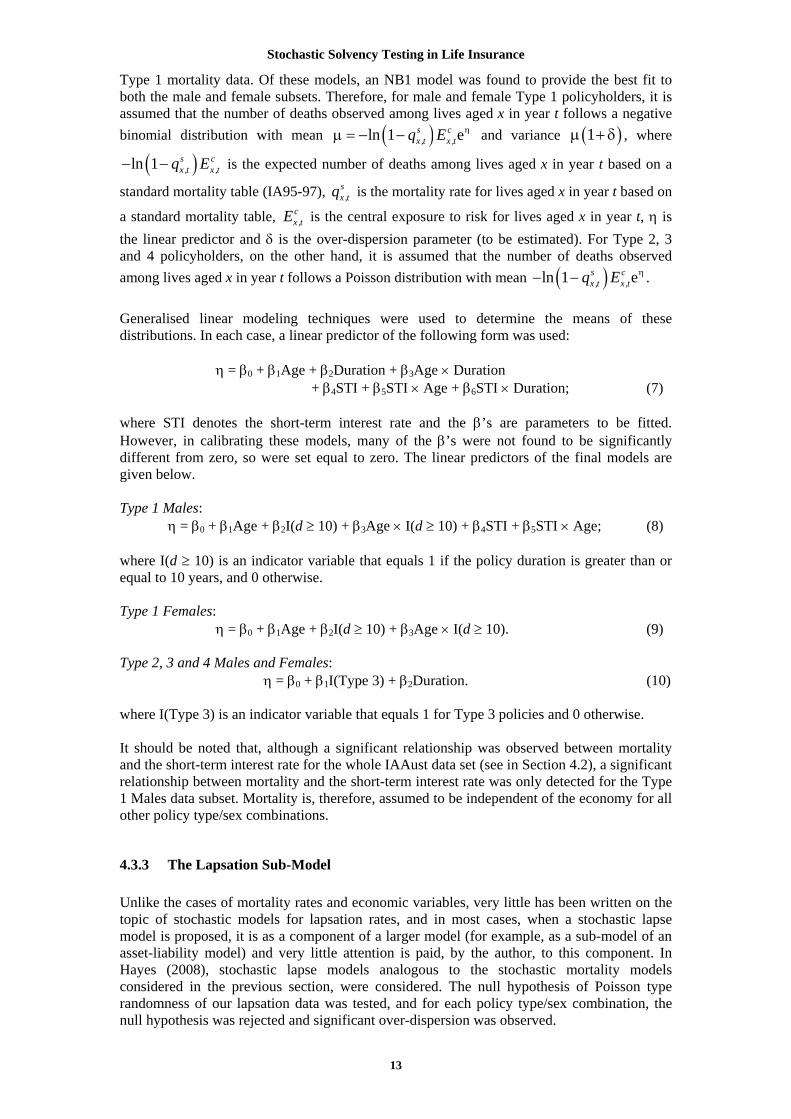
4.3.3 The Lapsation Sub-Model Unlike the cases of mortality rates and economic variables, very little has been written on the topic of stochastic models for lapsation rates, and in most cases, when a stochastic lapse model is proposed, it is as a component of a larger model (for example, as a sub-model of an asset-liability model) and very little attention is paid, by the author, to this component. In Hayes (2008), stochastic lapse models analogous to the stochastic mortality models considered in the previous section, were considered. The null hypothesis of Poisson type randomness of our lapsation data was tested, and for each policy type/sex combination, the null hypothesis was rejected and significant over-dispersion was observed.
13

Stochastic Solvency Testing in Life Insurance
A range of over-dispersion models were then considered for modelling the number of lapses at duration d in year t. It was subsequently decided to use a normal-Poisson model to model policy lapses for all policy type/sex combinations. That is, the number of policy lapses is assumed to follow a Poisson distribution with mean e es c
d ,t d ,tw E η ςμ = , where sd ,tw denotes the
lapsation rate at duration d in year t based on a “standard table” constructed in Hayes (2008) and c
d ,tE is the central exposure to risk among policies at duration d in year t, and ζ is a linear combination of normally distributed random coefficients. After removing any insignificant covariates from the model, the final version of the linear predictor was of the form:
η = β0 + β1Age + β2Duration + β3Sex + β4Type + β5Age × Duration + β6Age × Sex + β7Age × Type + β8Duration × Sex + β9Duration × Type + β10Sex × Type + β11U + β12U × Age + β13U × Duration + β14U × Type + β15STI + β16STI × Age + β17STI × Duration + β18STI × Sex + β19STI × Type; (11)
where U denotes the unemployment rate and Sex and Type were both fitted as categorical covariates. The linear combination of random coefficients was of the form: ζ = ψ0 + ψ1Sex + ψ2Type (12) where ( )2
i ~ N 0,ψ iσ , Cov(ψi, ψj) = σi,j, and the σ’s are parameters to be fitted.
5 Solvency Testing Methodology
5.1 Methodology In Section 4, we described three interconnected stochastic sub-models: an economic model, a mortality model and a lapsation model. These models are required in order to simulate input values to the solvency testing calculations. Once these models have been specified and calibrated, observations can be simulated and the insurer's capital at some future point in time can be found. Repeating this procedure a large number of times produces many estimates of the capital value which can be used to calculate an empirical distribution of the capital amount. From this distribution, solvency capital requirements can be found. This simulation-based approach was also used in Daykin et al. (1994), Lee (2000) and Tsai et al. (2001). The capital distribution, once estimated, is used to calculate target solvency capital amounts which can be compared with those calculated deterministically under the current Australian standards, as we do in Section 6. As mentioned in Section 2.1, a number of different methods can be used to determine solvency capital and there is no general consensus as to which of these methods is the most suitable. Consequently, we will consider two versions of the model, in which solvency capital is calculated using either the VaR or the TVaR method. The capital distribution can also be used to calculate the minimum value of assets that an insurer must hold at a particular point in time so that it satisfies its solvency capital requirement, holds sufficient funds so that its liabilities can be met, and could provide adequate risk compensation to a hypothetical insurer that may take over the portfolio in the future. This amount, which is referred to as the stochastic minimum asset requirement (SMAR), is calculated as:
SMAR = Best estimate liability + Cost of capital risk margin + Solvency capital requirement. (13)
This quantity is similar to the minimum asset requirement under the Swiss Solvency Test, although in this case, a credit margin is not included. 14

Stochastic Solvency Testing in Life Insurance
Solvency capital in the model is calculated using a 99.5% confidence level over a one year time horizon, in keeping with the recommendations of IAA (2004) and with precedents throughout the world8, and using a 95% confidence level over a three year time horizon, as this is the level of sufficiency that the current Australian Solvency standard is calibrated to (according to Karp (2002)). Below we describe the algorithm used to determine the 99.5% VaR and TVaR of –ΔC(1) and the 95% VaR and TVaR of –ΔCmin(0,3), where ΔC(1) denotes the increase in the insurer’s capital over a one year time horizon and ΔCmin(0,3) = min(ΔC(1), ΔC(0,2), and ΔC(0,3)). ΔC(0, t) denotes the increase in the insurer’s capital between time 0 (the valuation date) and time t (where t is given in years). It can be demonstrated (as was done in Hayes (2008)) that the 99.5% VaR of the distribution of –ΔC(1) is the amount of capital required at time t = 0 such that there is a 99.5% probability that the assets exceed the liability after one year (that is, at time t = 1). Similarly, it can be demonstrated that the 95% VaR of the distribution of –ΔCmin(0,3) is the amount of capital required at time t = 0 such that there is a 95% probability that the assets exceed the liabilities at each of the three times t = 1, 2 and 3. The algorithm is as follows:
1. (Deterministically) determine the value of the insurer's policy liabilities at time t = 0, denoted PL(0), using the methodology outlined in LPS1.04, but making no allowance for future shareholder profits.
2. Simulate the mortality, lapsation and economic experience over the period from t = 0
to t = 3 using the stochastic sub-models described in Section 4. 3. Assuming the experience simulated in Step 2, determine the value of the insurer's
policy liabilities at times t = 1, 2 and 3, denoted PL(1), PL(2) and PL(3) respectively, and the value of the insurer's net cash inflows at the beginning and the end of each year within the time period, CFboy(0,1), CFeoy(0,1), CFboy(1,2), CFeoy(1,2), CFboy(2,3), and CFeoy(2,3); and determine the rate of return on the insurer's assets between each of the balance dates in the period from time 0 to time 3, R(0,1), R(1,2) and R(2,3).
4. Using the results of Step 3, calculate ΔC(1), ΔC(0,2), and ΔC(0,3) using the
following formulae:
eoyboy
(0,1) (1)(1) (0) (0,1)
1 (0,1)CF PL
C PL CFR
−Δ = + +
+; (14)
eoyboy
(0,1) (1,2)(0,2) (0) (0,1)
1 (0,1)boyCF CF
C PL CFR−
Δ = + ++
eoy (1,2) (2)1 (0,2)
CF PLR
−+
+; (15)
and
eoyboy
(0,1) (1,2)(0,3) (0) (0,1)
1 (0,1)boyCF CF
C PL CFR−
Δ = + ++
eoy eoy(1,2) (2,3) (2,3) (3)1 (0,2) 1 (0,3)
boyCF CF CF PLR R− −
+ ++ +
; (16)
15
8 These were discussed in Section 2.2.

Stochastic Solvency Testing in Life Insurance
16
where
1 + R(0,2) = (1 + R (0,1))(1 + R (1,2)); (17)
and
1 + R(0,3) = (1 + R (0,1))(1 + R (1,2))(1 + R (2,3)). (18)
5. Determine ΔCmin(0,3) = min(ΔC(1), ΔC(0,2), and ΔC(0,3)). 6. Repeat Steps 2 – 5 a “large number” of times and from these simulated values of
ΔC(1) and ΔCmin(0,3), determine empirical probability distributions of –ΔC(1) and –ΔCmin(0,3) respectively.
7. Using the empirical distribution of –ΔC(1) determined in Step 6, calculate the 99.5%
VaR and the 99.5% TVaR, and similarly, using the empirical distribution of –ΔCmin(0,3), calculate the 95% VaR and the 95% TVaR.
In the above-given algorithm, it is necessary to simulate the mortality, lapsation and economic experience over the three year period under consideration; that is, to simulate numbers of deaths and withdrawals and values of each of the economic variables. This is done using the stochastic sub-models described in Section 4 and Latin Hypercube sampling (implemented using the @Risk simulation add-on for Microsoft Excel). In Step 6 of the algorithm, it is also required that Steps 2 – 5 of the algorithm be performed a “large number” of times (each repetition of these steps is referred to as an iteration). What is meant by this is that iterations should be performed until @Risk deems that “convergence” has occurred (that is, when the mean, standard deviation and selected percentile values of the output values of –ΔC(1) and –ΔCmin(0,3) do not change by more than 1% between calculations, where these statistics are recalculated every 100 iterations) and the number of iterations performed is large enough so that the statistics about the tails of the distribution can be calculated with a high level of accuracy (the 99.5% quantile of the distribution of –ΔC(1) is estimated within ± 5% of its true value with 95% confidence and similarly for the 95% quantile of the distribution of –ΔCmin(0,3)). Most of the calculations performed in determining –ΔC(1) and –ΔCmin(0,3) are performed using cash-flow projection techniques, implemented using spreadsheet models (for example, the calculation of PL(1) in Step 3 of the algorithm). All spreadsheet models required for this paper were built using Microsoft Excel and are described in detail in Hayes (2008).
5.2 Assumptions In implementing the spreadsheet models referred to in Section 5.1, it is necessary to make a number of deterministic input assumptions. The assumptions were chosen to represent a typical Australian Life Insurer and the most pertinent assumptions are discussed below.
5.2.1 Portfolio Specifications The results of the analysis carried out in this paper may potentially change, depending on the composition of the insurance portfolio under consideration. That is, the policy type represented in the portfolio; the durations and sums insured of the policies; and the age and sex distribution of the policyholders. We do not attempt to consider every possible age/sex/type/sum insured/duration combination in this paper. Instead, a small number of model portfolios have been constructed, each containing policies that fit into one of a relatively small number of groups defined by age, sex, type, sum insured and duration.

Stochastic Solvency Testing in Life Insurance
Four model portfolios were constructed, each containing policies of only a single type, with the age and sex composition of each portfolio determined by reference to what was observed in the IAAust data set. Table 1 gives the composition of each portfolio. It is assumed that within each age band all policies are held by policyholders of an age equal to the mid-point of the age band under consideration, rounded to the nearest integer. For example, all lives in the 15 – 24 year age band are assumed to be exactly 20 years of age (for the 75+ years age band, all policyholders are assumed to be exactly 80 years old).
Table 1: Model Portfolio Compositions
Type 1 Type 2 Type 3 Type 4Males 15 - 24 3.00% 2.72% 0.55% 0.62%
25 - 34 9.00% 17.00% 7.70% 10.54%35 - 44 16.50% 25.84% 17.60% 22.94%45 - 54 22.50% 18.36% 21.45% 21.70%55 - 64 15.00% 4.08% 7.70% 6.20%65 - 74 5.25% 0.00% 0.00% 0.00%75+ 3.75% 0.00% 0.00% 0.00%
Females 15 - 24 2.00% 1.60% 0.45% 0.76%25 - 34 4.25% 8.00% 8.10% 9.12%35 - 44 6.75% 12.48% 21.15% 16.72%45 - 54 6.75% 8.64% 13.05% 9.88%55 - 64 3.00% 1.28% 2.25% 1.52%65 - 74 1.25% 0.00% 0.00% 0.00%75+ 1.00% 0.00% 0.00% 0.00%
Total 100.00% 100.00% 100.00% 100.00%
All Type 1 policies are assumed to be (non-participating) endowment insurance policies with terms of length such that the policies mature on the policyholder's 100th birthday, if the policy is still in force at that date (this is effectively the same as a whole of life insurance policy, but ignores ages greater than 100, for which mortality rates are not tabulated); Type 2 policies are assumed to be investment-linked policies, all surrendered at age 65 exact, provided prior surrender or death has not already occurred; and all Type 3 and 4 policies (level term insurance and yearly renewable term insurance respectively) are also assumed to expire on the policyholder's 65th birthday. A policy expiry age of 65 was selected for Type 2, 3 and 4 policies because an analysis of the IAAust Data Set shows that there is a marked decrease in the exposures for these policy types at ages greater than 65. For each of these policy types, less than 1% of all policies are held by lives aged 65 or above. APRA(2007) shows that most Type 1, 3 and 4 policies are paid for by regular premiums (that is, premiums that are payable at regular intervals throughout the life of the policy), while, for investment-linked business, the majority of policies are single premium policies. Thus, in this paper, Type 1, 3 and 4 policies are all assumed to be regular premium policies, while Type 2 policies are assumed to be single premium policies. The policy duration for each age/sex/policy type combination is assumed to be equal to the average duration (rounded to the nearest integer) for the age band, sex and policy type under consideration, based on the Single Insurer Mortality data set (this is the only data set for which sufficient information is given to make such assumptions). As the Single Insurer data does not include Type 2 or 3 policies, the same duration assumptions were made for Type 1 and 3 policies (both of which are “traditional” policy types) and for Type 2 and 4 policies (both of which are “modern” policy types). These duration assumptions are given in Table 2. For all policy types, policyholders' birthdays are assumed to coincide with the policy 17

Stochastic Solvency Testing in Life Insurance
anniversaries, which are assumed to coincide with the solvency testing date. Note that no allowance is made for new policies that the insurer might sell during the solvency testing time period, since no such allowance is made in LPS2.04 and new business is only allowed for in LPS3.04 via the new business reserve. New business is also ignored in the Swiss Solvency Test, upon which the stochastic solvency testing model developed in this paper is largely based.
Table 2: Duration Assumptions (Years) by Age Band, Sex and Policy Type
Types 1 & 3 Types 2 & 4 Types 1 & 3 Types 2 & 415 - 24 17 4 17 425 - 34 22 3 22 335 - 44 22 5 20 545 - 54 26 7 22 755 - 64 30 8 25 865 - 74 36 - 29 -75+ 43 - 35 -
Males Females
For consistency, all Type 1, 3 and 4 policies are assumed to have the same sum insured. The average sum insured of policies in the Single Insurer Mortality data set is $116,217.32. This value was rounded to the nearest $10,000 to get the sum insured assumption of $120,000. For investment-linked (Type 2) policies, premiums are used to purchase units in a managed fund and death benefits depend on the value of these units at the time of the policyholder's death (that is, the accumulated value of premiums received to date at the investment earnings rate, less fees and tax on investment earnings). In the Type 2 policy cases the single premium is set such that the expected policy benefit at age 65 is $120,000.
5.2.2 Asset Mix The composition of the portfolio of assets backing an insurer's liabilities depends on a number of factors including, among other things, the insurer's attitude to risk, solvency considerations, the nature of the liabilities and any promises made in the policy documentation. Typically, however, risk-based insurance policies (including Type 3 and 4 policies) will be backed by cash (that is, short-term (less than one year) fixed interest investments, such as 90 day Commonwealth Government bills) and (long-term) fixed interest securities, while traditional savings-based insurance policies (Type 1 policies) will be backed by a mixture of long-term growth assets and fixed interest securities (and some cash, for liquidity purposes). For Type 2 policies, policyholders will generally be given a choice of investment options at policy inception and the assets backing a portfolio of Type 2 policies will reflect this choice. For the purposes of this paper, four model asset portfolios (which are subsequently referred to as Portfolios 1, 2, 3 and 4) were constructed based on the “typical” investment fund mixes suggested in Choice (2007) and with reference to the investment options offered by Australia's five largest Life Insurers9 for their investment-linked business (as stated on their respective internet sites). Table 3 gives the percentage weightings for each of the four main asset classes (equities, property, fixed interest securities and cash) in each of these portfolios. Portfolio 1 is an example of a very low risk, bond, portfolio; Portfolio 2 is an example of a low risk, “capital stable”, portfolio; Portfolio 3 is an example of a medium risk, “balanced”, portfolio; and Portfolio 4 is an example of a high risk, “growth”, portfolio. In this paper, it is assumed that Type 3 and 4 policies are backed by a Portfolio 1 asset mix and Type 1 policies
18
9 According to APRA (2007), Australia’s five largest Life Insurers by statutory fund assets are: AMP, National Australia Bank/MLC, ING/ANZ, Colonial/Commonwealth Bank of Australia, and National Mutual/AXA.

Stochastic Solvency Testing in Life Insurance
are backed by a Portfolio 3 asset mix. Type 2 policyholders are assumed to have been given a choice between the four different investment options proposed in Table 3, and all Type 2 policy calculations were repeated four times, once for each of these asset mixes.
Table 3: Composition of each of the Model Asset Portfolios
Portfolio 1 Portfolio 2 Portfolio 3 Portfolio 4Equity 0% 25% 55% 75%
Property 0% 5% 5% 5%Fixed Interest 70% 45% 30% 15%
Cash 30% 25% 10% 5%Total 100% 100% 100% 100%
5.3 Sensitivity Analysis Throughout this paper, every effort has been made to devise the most realistic sub-models and assumptions possible. However, determining these is a time consuming process, and in practice, an insurer might not have the time or expertise necessary to make such decisions. Sensitivity testing is, therefore, conducted to investigate the impact on the model outputs and the resulting solvency capital requirements of using different stochastic sub-models, being simplified versions of those previously described. Thus, in addition to comparing the impact of using different economic sub-models, the impact on the results of each of the following model variants is also investigated:
1. Assume that deaths follow a Poisson distribution, instead of a negative binomial distribution, for Type 1 policies, with the mean of the Poisson distribution set equal to the mean of the negative binomial distribution in each case.
2. Assume that lapses follow a Poisson distribution, instead of modelling them using the
normal-Poisson model, with the mean of the Poisson distribution set equal to the mean under the normal-Poisson model.
3. Assume both Variants 1 and 2 at the same time, in the case of Type 1 policies.
4. Assume that deaths and lapses are both Poisson distributed and that the means of
these distributions do not vary with fluctuations in the economic variables. In this case, the latter is achieved by calculating those means from the formulae used to calculate them under the best-fitting model scenarios, but replacing the values of the economic variables at time t with the averages of the forecast values of those quantities for the first 10 years after the solvency testing date, forecast using the economic sub-model under consideration in each case. This is done to keep the functional relationships used to relate the means of the mortality rates and lapsation rates with the economic variables similar to those used in Variants 1 to 3.
5. Assume that, for each policy type/sex combination, deaths and lapses are both
Poisson distributed with means equal to ( )ln 1 s cx ,t x ,t dq E− − α and s c
d ,
respectively, where αd and αw are constants that vary only by policy type and sex, but not by age, duration or with fluctuations in the economy.
t d ,t ww E α
All five of these variants are considered in order to investigate the impact on the results of ignoring the existence of over-dispersion in the mortality and/or lapsation sub-models, and Variants 4 and 5 are considered in order to investigate the impact of ignoring dependencies between the three stochastic sub-models. Variant 5 is considered because many insurers simply assume that the mean mortality rates used in insurance calculations are a constant 19

Stochastic Solvency Testing in Life Insurance
multiple of the rates given in a standard mortality table (such as IA95-97 M and F), where the constant varies only by policy type and sex, and that lapsation rates vary only by policy type and duration (lapsation rates are, here, also allowed to vary by sex for consistency with the mortality model). Variant 5 allows the impact of making such simple mean assumptions to be investigated. Note that, because αd and αw do not depend on any of the economic variables, no allowance is made for the previously observed (and allowed for) dependencies between the mortality rates and economic variables, and between the lapse rates and economic variables. Suitable values of αd and αw were estimated by fitting Poisson GLMs to the IAAust Mortality Data (for αd) and the Single Insurer Mortality Data (for αw) respectively, in each case with a linear predictor of the form:
η = β0 + β1Type + β2Sex + β3Type × Sex; (19)
where (policy) type and sex are treated as categorical covariates and the β's are model parameters to be estimated. The values of αd and αw are then set equal to , where is the fitted value of the linear predictor for the model under consideration.
ˆeη η̂
6 Results In Section 5, we described a simulation-based solvency testing methodology. This methodology was implemented using the assumptions specified in Section 5 and using the stochastic sub-models described in Section 4, including the modified CAS/SOA economic sub-model (which was found to provide the best fit to the economic data). This process was then repeated, assuming each of the other economic sub-models previously considered and using different mortality and lapsation sub-models, as outlined in Section 5.3, in order to perform sensitivity analyses of the results. The purpose of this analysis is to determine how the solvency and capital adequacy requirements calculated deterministically under LPS2.04 and LPS3.04, respectively, compare with the solvency capital requirements calculated using the stochastic solvency testing model; how these deterministic requirements compare with the stochastic minimum asset requirements; and whether these results are affected by sensitivity changes to the stochastic solvency testing model. The results of this analysis are presented and discussed in this section.
6.1 Base Case Simulation Results The variables we focus on are the change in capital over a one year time horizon, ΔC(1), and ΔCmin(0,3) = min(ΔC(1), ΔC(0,2), and ΔC(0,3)), the smallest increase in capital over a three year time horizon. In the stochastic solvency model, these variables are assumed random with the distributions for the stochastic sub-models that were, in Hayes (2008), shown to best describe the mortality, lapsation and economic data (that is, the NB1 or Poisson mortality models for mortality, the normal-Poisson lapsation model for lapsation and the modified CAS/SOA economic model for economic variables such as interest rates, inflation, etc). Values of ΔC(1), and ΔCmin(0,3) were simulated for each liability portfolio/asset portfolio combination as described in Section 5. This scenario is subsequently referred to as the “Base Case”. Based on the simulation outputs, the 99.5% VaR and TVaR per policy of –ΔC(1), and the 95% VaR and TVaR per policy of –ΔCmin(0,3) were calculated empirically for each of the portfolios under consideration. As a basis for comparison, the LPS2.04 solvency capital requirement per policy and LPS3.04 capital adequacy capital requirement per policy10, for
20
10 Recall that the solvency capital requirement was defined in Section 2.2 as the difference between the LPS2.04 solvency requirement and the best estimate liability; and the capital

Stochastic Solvency Testing in Life Insurance
each portfolio, were also calculated. These quantities are compared in Figure 2. Note that in this graph, Portfolio 2.1 refers to the Type 2 liability portfolio backed by a Type 1 asset portfolio, and similarly for Portfolios 2.2, 2.3 and 2.4. Note also that, in all but one case, there is no difference between the LPS2.04 solvency capital requirement and the LPS3.04 capital adequacy capital requirement. This is because the LPS3.04 capital adequacy requirement is equal to the maximum of the LPS2.04 solvency requirement and the amount calculated in Item (f) of the LPS3.04 methodology plus the new business reserve. Under the assumptions made in performing these simulations, in all cases the new business reserve is zero, and in most cases the LPS2.04 solvency reserve is greater than the amount calculated in Item (f) of the LPS3.04 methodology. Thus, in each of these cases, the LPS3.04 capital adequacy requirement is equal to the LPS2.04 solvency requirement, and the capital adequacy capital requirement is equal to the solvency capital requirement.
-2000
0
2000
4000
6000
8000
10000
12000
1 2.1 2.2 2.3 2.4 3 4
Portfolio
99.5% VaR99.5% TVaR95% VaR95% TVaRLPS 2.04 Cap. Req.LPS 3.04 Cap. Req.
Figure 2: Capital Requirements per Policy for the Base Case Scenarios ($)
From Figure 2, it can be seen that, in all cases, as expected, the 100(1 – α)% TVaR is greater than the corresponding 100(1 – α)% VaR. However, for all portfolios containing Type 1 or Type 2 policies, the 99.5% VaR of the distribution of –ΔC(1) is greater than the 95% VaR of the distribution of –ΔCmin(0,3), and the the 99.5% TVaR of the distribution of –ΔC(1) is greater than the 95% TVaR of the distribution of –ΔCmin(0,3), which is a more surprising result. In the Type 2 policy cases, this arises from the fact that, for each asset portfolio scenario, ΔC(1) = ΔCmin(0,3) at every iteration, resulting in the empirical distributions of –ΔC(1) and –ΔCmin(0,3) being identical. For any given probability distribution, the 95th percentile will always be less than the 99.5th percentile. For the Type 3 and 4 policy portfolios, however, the 99.5% VaR of the distribution of –ΔC(1) is much less than the 95% VaR of the distribution of –ΔCmin(0,3) and similarly for the TVaRs. For several of the Type 2 policy cases, the VaR and/or the TVaR capital amounts shown in Figure 2 are negative, particularly when a more conservative asset allocation is employed. This implies that, in these cases, even if an insurer held no capital at time 0, it is almost certain that the insurer will remain solvent into the future. This reflects the extremely low risk to the insurer associated with investment-linked insurance policies. Comparing the VaR and TVaR capital amounts with the LPS2.04 and LPS3.04 capital amounts (the Solvency Capital Requirement and the Capital Adequacy Capital Requirement respectively), it can be seen that for Type 1 and 2 policies, the LPS2.04 and LPS3.04 amounts are much greater than the corresponding VaR and TVaR amounts, while for Type 3 policies,
21
adequacy capital requirement was similarly defined as the difference between the LPS3.04 capital adequacy requirement and the best estimate liability.

Stochastic Solvency Testing in Life Insurance
the LPS2.04 and LPS3.04 amounts are less than the VaR and TVaR amounts. For Type 4 policies, the LPS2.04 and LPS3.04 amounts are greater than the 99.5% VaR and TVaR amounts, but less than the 95% values. The levels of sufficiency (on a VaR basis) of each of the LPS2.04 and LPS3.04 capital amounts are given in Table 4. For portfolios containing Type 1 or 2 policies, this level is greater than 99.99%, when compared to either the empirical distribution of –ΔC(1) or –ΔCmin(0,3). In the cases of portfolios containing Type 3 or 4 policies, however, the levels of sufficiency (on a VaR basis) are often much lower, and are less than 5% in all cases when solvency is considered over a three year time horizon. Note that, if calculated on a TVaR basis, the sufficiency levels would be slightly lower than those calculated on a VaR basis.
Table 4: Levels of Sufficiency (on a VaR Basis) of the LPS2.04 and LPS3.04 Capital Requirements for the Base Case Scenarios
Liability AssetPortfolio Portfolio LPS2.04 LPS3.04 LPS2.04 LPS3.04
1 3 >99.99% >99.99% >99.99% >99.99%2 1 >99.99% >99.99% >99.99% >99.99%2 2 >99.99% >99.99% >99.99% >99.99%2 3 >99.99% >99.99% >99.99% >99.99%2 4 >99.99% >99.99% >99.99% >99.99%3 1 1.36% 72.45% 0.00% 1.19%4 1 >99.99% >99.99% 0.00% 0.00%
−ΔC(1) −ΔCmin(0,3)
The implication of these results is that the current Australian solvency and capital adequacy requirements do not provide the same level of protection against insolvency for all types of life insurance business, and for some classes of business, provide very little long term protection against insolvency at all. We set the (stochastic) minimum asset requirement for an insurer equal to the 100(1 – α)% VaR (or TVaR) plus the corresponding cost of capital (CoC) risk margin (calculated using the methodology set out in CEA (2006) and FOPI (2006) and using the assumptions set out in Hayes (2008)) plus the best estimate liability. Table 5 gives the ratios of the LPS2.04 and LPS3.04 solvency and capital adequacy requirements (that is, the LPS2.04 and LPS3.04 capital requirements plus the best estimate liabilities) to each of these quantities. From this table, it can be seen that the existing deterministic solvency and capital adequacy legislation requires insurers to hold 12 – 34% more assets for Type 1 and 2 policies than would be required under the hypothetical stochastic scenario, but for Type 3 and 4 policies, the deterministic requirements are less than 80% of the stochastic requirements (and for the Type 4, three year time horizon cases, less than 10%). Note that the negative ratios in this table arise from the fact that, for Type 4 policies, the LPS2.04 and LPS3.04 requirements are positive, while the stochastic asset requirements calculated based on the empirical distribution of –ΔC(1) are negative. In each of these cases, the LPS2.04 and LPS3.04 requirements are, needless to say, more than adequate.
22

Stochastic Solvency Testing in Life Insurance
Table 5: Ratios of the LPS2.04 and LPS3.04 Solvency and Capital Adequacy Requirements to the Stochastic Minimum Asset Requirements for the Base Case Scenarios
Liability AssetPortfolio Portfolio 99.5% VaR 99.5% TVaR 95% VaR 95% TVaR
Solvency Requirement (LPS2.04) Ratios1 3 126% 123% 131% 126%2 1 112% 112% 113% 113%2 2 121% 121% 122% 122%2 3 126% 125% 130% 128%2 4 130% 129% 134% 132%3 1 54% 53% 41% 40%4 1 -8% -9% 6% 6%
Capital Adequacy Requirement (LPS3.04) Ratios1 3 126% 123% 131% 126%2 1 112% 112% 113% 113%2 2 121% 121% 122% 122%2 3 126% 125% 130% 128%2 4 130% 129% 134% 132%3 1 79% 76% 60% 58%4 1 -8% -9% 6% 6%
−ΔC(1) −ΔCmin(0,3)
6.2 Sensitivity Analysis
6.2.1 Economic Sub-Model Sensitivities In determining the “most appropriate” economic sub-model to include in the stochastic solvency testing model, four different economic sub-models were compared: the Kemp model, the Wilkie model, the CAS/SOA model and the modified CAS/SOA model. Ultimately, it was concluded that the modified CAS/SOA model provided the best fit to the data, and consequently, this economic model was used in the Base Case tests described in the previous section. In this section, we consider the impact on the results of using either the Kemp, Wilkie or CAS/SOA economic models in place of the modified CAS/SOA model, all other things being equal. As in the Base Case scenarios, values of –ΔC(1) and –ΔCmin(0,3) were simulated for each economic model/liability portfolio/asset portfolio combination. After enough iterations had been performed for the summary statistics of these quantities to converge as per the @Risk algorithm, two-sample Kolmogorov-Smirnov tests were conducted to test the null hypothesis that these samples were drawn from the same probability distributions as the Base Case samples for the same liability portfolio/asset portfolio combination. The p-values of these tests are given in Table 6. In all but four cases, the null hypothesis is rejected at the 5% significance level for both the simulated values of –ΔC(1) and of –ΔCmin(0,3). This is strong evidence that using a different economic sub-model does have a significant impact on the distribution of the simulation outputs.
23

Stochastic Solvency Testing in Life Insurance
Table 6: p-values for the Two-Sample Kolmogorov-Smirnov Tests for the Economic Sub-Model Sensitivity Scenarios
Liability Asset EconomicPortfolio Portfolio Model
1 3 Kemp 0.000* 0.000*1 3 Wilkie 0.000* 0.000*1 3 CAS/SOA 0.000* 0.000*2 1 Kemp 0.000* 0.000*2 1 Wilkie 0.701 0.7012 1 CAS/SOA 0.000* 0.000*2 2 Kemp 0.000* 0.000*2 2 Wilkie 0.007* 0.007*2 2 CAS/SOA 0.039* 0.039*2 3 Kemp 0.000* 0.000*2 3 Wilkie 0.000* 0.000*2 3 CAS/SOA 0.000* 0.000*2 4 Kemp 0.000* 0.000*2 4 Wilkie 0.000* 0.000*2 4 CAS/SOA 0.000* 0.000*3 1 Kemp 0.000* 0.000*3 1 Wilkie 0.000* 0.000*3 1 CAS/SOA 0.000* 0.000*4 1 Kemp 0.000* 0.000*4 1 Wilkie 0.727 0.8474 1 CAS/SOA 0.000* 0.000*
−ΔC(1) −ΔCmin(0,3)
Note: * indicates significance at the 5% significance level.
Where necessary, additional simulation runs were performed to ensure that the accuracy criteria for the quantiles were met, and based on these final sets of simulated outputs, the VaR and TVaR per policy were calculated for each scenario under consideration. Figures 3 to 5 show these quantities, plotted alongside the LPS2.04 and LPS3.04 capital requirements for each economic sub-model.
-2000
0
2000
4000
6000
8000
10000
12000
1 2.1 2.2 2.3 2.4 3 4
Portfolio
99.5% VaR99.5% TVaR95% VaR95% TVaRLPS 2.04 Cap. Req.LPS 3.04 Cap. Req.
Figure 3: Capital Requirements per Policy Using a Kemp Economic Sub-Model ($)
24

Stochastic Solvency Testing in Life Insurance
-2000
0
2000
4000
6000
8000
10000
12000
1 2.1 2.2 2.3 2.4 3 4
Portfolio
99.5% VaR99.5% TVaR95% VaR95% TVaRLPS 2.04 Cap. Req.LPS 3.04 Cap. Req.
Figure 4: Capital Requirements per Policy Using a Wilkie Economic Sub-Model ($)
-2000
0
2000
4000
6000
8000
10000
12000
1 2.1 2.2 2.3 2.4 3 4
Portfolio
99.5% VaR99.5% TVaR95% VaR95% TVaRLPS 2.04 Cap. Req.LPS 3.04 Cap. Req.
Figure 5: Capital Requirements per Policy Using a CAS/SOA Economic Sub-Model ($) Comparing the VaR and TVaR amounts to the LPS2.04 and LPS3.04 solvency and capital adequacy capital requirement amounts, it can be seen that, again, the Type 1 and 2 policy LPS2.04 and LPS3.04 capital requirements are greater than the corresponding VaR and TVaR amounts; the Type 3 LPS2.04 and LPS3.04 capital requirements are, in most cases, less than the VaR and TVaR amounts; and the Type 4 LPS2.04 and LPS3.04 capital requirements are greater than the 99.5% VaR and TVaR amounts, but less than the 95% quantities. In all cases, the LPS2.04 and LPS3.04 capital amounts are greater than the 99.99% sufficiency level (on a VaR basis) for Type 1 and 2 policies, but the sufficiency levels are, again, generally much lower for Type 3 and 4 policies. The CoC risk margins were calculated for each scenario, using each of the solvency capital requirements under consideration and these risk margins were then added to the best estimate liabilities and VaR or TVaR values, as was done in Section 6.1, to get the stochastic asset requirements. Although, as has been previously mentioned, the use of different economic sub-models, in most cases, gives rise to simulated values of –ΔC(1) and –ΔCmin(0,3) that follow significantly different distributions from their Base Case equivalents, when the best estimate liabilities, CoC risk margins and VaR (or TVaR) values are combined to give the stochastic asset requirements, for most liability portfolio/asset portfolio combinations, varying the 25

Stochastic Solvency Testing in Life Insurance
economic sub-model used has very little impact on the results. Table 7 gives the ratios of the sensitivity analysis asset requirements to the Base Case requirements for the same portfolio, and in all but 15 out of the 84 cases considered, the ratio is between 95% and 105%. All of the scenarios for which the ratio falls outside the 95 – 105% range relate to Type 3 or 4 policies, and mostly to Type 3 policies (12 out of the 15 cases where the ratio falls outside this range). In 13 of these 15 cases, the ratios are greater than 100%, implying higher minimum asset requirements than under the Base Case scenarios; and in the two remaining cases, although the ratios in these cases are less than 100%, because the minimum asset requirements are negative, the ratios also imply higher minimum asset requirements than under the Base Case scenarios.
Table 7: Ratios of the Economic Sub-Model Sensitivity Analysis Stochastic Minimum Asset Requirements to the Base Case Requirements for the Same Portfolio
Liability Asset EconomicPortfolio Portfolio Model 99.5% VaR 99.5% TVaR 95% VaR 95% TVaR
1 3 Kemp 103% 103% 102% 101%1 3 Wilkie 102% 102% 100% 99%1 3 CAS/SOA 100% 100% 97% 96%2 1 Kemp 102% 102% 102% 102%2 1 Wilkie 100% 100% 100% 100%2 1 CAS/SOA 101% 101% 100% 100%2 2 Kemp 102% 102% 103% 102%2 2 Wilkie 100% 100% 100% 100%2 2 CAS/SOA 100% 99% 100% 100%2 3 Kemp 102% 101% 102% 102%2 3 Wilkie 100% 100% 100% 100%2 3 CAS/SOA 99% 99% 99% 99%2 4 Kemp 101% 101% 102% 102%2 4 Wilkie 99% 99% 100% 100%2 4 CAS/SOA 98% 98% 99% 99%3 1 Kemp 112% 109% 119% 116%3 1 Wilkie 118% 118% 115% 115%3 1 CAS/SOA 138% 139% 125% 126%4 1 Kemp 85% 85% 98% 97%4 1 Wilkie 99% 99% 100% 100%4 1 CAS/SOA 96% 95% 105% 106%
−ΔC(1) −ΔCmin(0,3)
When the LPS2.04 and LPS3.04 solvency and capital adequacy requirements are compared to the stochastic minimum asset requirements, similar observations are made to those that were made in Section 6.1. Thus, regardless of which economic sub-model is used, it still remains the case that for Type 1 and 2 policies, the LPS2.04 and LPS3.04 requirements are more than adequate and for Type 3 and 4 policies, in many cases, the LPS2.04 and LPS3.04 requirements are less than adequate.
6.2.2 Mortality Sub-Model Sensitivities In Hayes (2008), evidence was found to indicate the presence of over-dispersion in the Type 1 policy mortality data, and it was concluded that the best way of allowing for this over-dispersion in the mortality sub-model is by assuming that the number of deaths follows a negative binomial (NB1) distribution instead of the traditional Poisson distribution. In this section, we consider the impact of assuming that Type 1 policy mortality does, in fact, follow a Poisson distribution (with mean equal to the mean of the NB1 distribution), that is, of 26

Stochastic Solvency Testing in Life Insurance
27
making no allowance for over-dispersion. This is done assuming each of the four economic sub-models, not just the Base Case, modified CAS/SOA, model. Values of –ΔC(1) and –ΔCmin(0,3) for the Type 1 policy portfolio were once again simulated for each economic model scenario until enough iterations had been performed for the summary statistics of these quantities to converge as per the @Risk algorithm. Two-sample Kolmogorov-Smirnov tests were then conducted to test the null hypothesis that these samples were drawn from the same probability distributions as the samples simulated in Section 6.2.1 (the scenarios considered in Section 6.2.1 are subsequently referred to as the “Economic Base Case Scenarios”). In none of these tests is the null hypothesis that the two samples were drawn from the same probability distribution rejected at the 5% significance level. Consequently, it is concluded that ignoring the presence of over-dispersion in the mortality sub-model does not have a significant effect on the overall results.
6.2.3 Lapsation Sub-Model Sensitivities Similarly to what was done in Section 6.2.2, in this section we consider the impact on the results of assuming that lapses follow a Poisson distribution (with mean equal to the mean of the normal-Poisson lapsation model), instead of the normal-Poisson model that was shown, in Hayes (2008), to best describe the lapse data. Values of –ΔC(1) and –ΔCmin(0,3) were simulated for each economic model/liability portfolio/asset portfolio combination until convergence was achieved with the @Risk algorithm, and two-sample Kolmogorov-Smirnov tests were conducted to compare the distributions of these values with those of the Economic Base Case outputs. p-values of these tests are given in Table 8. From Table 8, it can be seen that, in most cases (50 out of the 56 cases considered) there is no significant evidence to suggest that the outputs simulated in this section are drawn from different distributions than their Economic Base Case counterparts. In 50 independent tests at the 5% significance level, we would expect 2.5 significant results by chance, even if the null hypothesis were correct. The six cases with p-values less than 0.05 exceed this, however, so we consider them further. Five out of these six cases assume a Kemp economic sub-model, suggesting that, if this economic sub-model is used, the results are more sensitive to the choice of lapsation sub-model than if an alternative sub-model is used. In none of these cases was it necessary to perform additional simulation trials in order to meet the accuracy criteria for the quantiles. For each of these, significantly different, cases, the VaR and TVaR values were calculated and the ratios of these quantities to their Economic Base Case counterparts are presented in Table 9. In some cases, particularly the Type 2 policy cases, the stochastic capital requirements do change substantially, in percentage terms, when the Poisson lapsation sub-model is used. For each of the six cases where the output distribution is believed to significantly differ from the equivalent Economic Base Case output distribution, the level of sufficiency of the LPS2.04 and LPS3.04 capital requirements was calculated (on a VaR basis). The sufficiency levels are all within ±2% of their Economic Base Case counterparts. The stochastic asset requirements were also calculated for each of the six cases under consideration. Comparing these values to the equivalent Economic Base Case values, in all cases the lapsation sub-model sensitivity values are within ±5% of the Economic Base Case values.
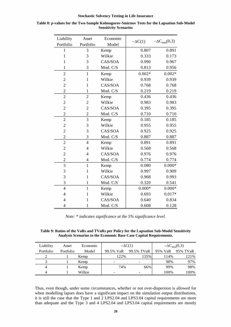
Stochastic Solvency Testing in Life Insurance
Table 8: p-values for the Two-Sample Kolmogorov-Smirnov Tests for the Lapsation Sub-Model Sensitivity Scenarios
Liability Asset EconomicPortfolio Portfolio Model
1 3 Kemp 0.807 0.8911 3 Wilkie 0.333 0.1731 3 CAS/SOA 0.990 0.9671 3 Mod. C/S 0.813 0.9562 1 Kemp 0.002* 0.002*2 1 Wilkie 0.939 0.9392 1 CAS/SOA 0.768 0.7682 1 Mod. C/S 0.219 0.2192 2 Kemp 0.436 0.4362 2 Wilkie 0.983 0.9832 2 CAS/SOA 0.395 0.3952 2 Mod. C/S 0.710 0.7102 3 Kemp 0.185 0.1852 3 Wilkie 0.955 0.9552 3 CAS/SOA 0.925 0.9252 3 Mod. C/S 0.887 0.8872 4 Kemp 0.891 0.8912 4 Wilkie 0.568 0.5682 4 CAS/SOA 0.976 0.9762 4 Mod. C/S 0.774 0.7743 1 Kemp 0.080 0.000*3 1 Wilkie 0.997 0.9093 1 CAS/SOA 0.968 0.9933 1 Mod. C/S 0.320 0.5414 1 Kemp 0.000* 0.000*4 1 Wilkie 0.693 0.017*4 1 CAS/SOA 0.640 0.8344 1 Mod. C/S 0.608 0.128
−ΔC(1) −ΔCmin(0,3)
Note: * indicates significance at the 5% significance level.
Table 9: Ratios of the VaRs and TVaRs per Policy for the Lapsation Sub-Model Sensitivity Analysis Scenarios to the Economic Base Case Capital Requirements.
Liability Asset EconomicPortfolio Portfolio Model 99.5% VaR 99.5% TVaR 95% VaR 95% TVaR
2 1 Kemp 122% 135% 114% 121%3 1 Kemp - - 98% 97%4 1 Kemp 74% 66% 99% 98%4 1 Wilkie - - 100% 100%
−ΔC(1) −ΔCmin(0,3)
Thus, even though, under some circumstances, whether or not over-dispersion is allowed for when modelling lapses does have a significant impact on the simulation output distributions, it is still the case that the Type 1 and 2 LPS2.04 and LPS3.04 capital requirements are more than adequate and the Type 3 and 4 LPS2.04 and LPS3.04 capital requirements are mostly
28

Stochastic Solvency Testing in Life Insurance
29
less than adequate; and in spite of the differences in the output distributions, there is little difference in the minimum assets that must be held under these scenarios compared to the Economic Base Case requirements.
6.2.4 Mortality and Lapsation Sub-Model Sensitivities Combining the sensitivity tests carried out in the previous two sections, in this section we investigate the impact on the results of assuming that both deaths and lapses follow Poisson distributions (with means equal to the means of the Base Case NB1 mortality model and the normal-Poisson lapse model respectively), for Type 1 policies. Values of –ΔC(1) and –ΔCmin(0,3) were simulated until convergence was reached with the @Risk algorithm for each economic model under this new scenario, and two-sample Kolmogorov-Smirnov tests were conducted to compare the distributions of these ouputs with those of the Economic Base Case outputs. This time, none of the tests lead to the rejection of the null hypothesis at the 5% significance level, providing strong evidence that, for Type 1 policies, ignoring the existence of any over-dispersion present in either the mortality or lapsation data has little effect on capital requirements.
6.2.5 Dependency Sensitivities In this section, we extend the sensitivity tests carried out in the previous three sections to investigate the impact of ignoring the existence of any dependency relationships between the economic variables, mortality and lapsation rates, in addition to assuming that mortality and lapses follow Poisson distributions. The functional relationships used to relate the means of the mortality and lapsation Poisson distributions with the economic variables remain similar in shape to those used to describe the means of the Base Case mortality and lapsation distributions (which are the same as those used to describe the means of the distributions used in Sections 6.2.2 to 6.2.4) but without allowing them to change as the economic variables change (the methodology used for doing this is described in Section 5.3). Values of –ΔC(1) and –ΔCmin(0,3) were simulated until convergence was reached with the @Risk algorithm for each economic model/liability portfolio/asset portfolio combination, and two-sample Kolmogorov-Smirnov tests were conducted to compare the distributions of the outputs to those of the Economic Base Case Scenarios, with p-values given in Table 10. In 21 of the 56 cases presented, the null hypothesis is rejected at the 5% significance level, with most of these cases reflecting Type 1, 3 or 4 policies. This suggests that, for these policy types, allowing for the existence of dependency relationships between mortality, lapsation and the economy may have a significant effect on the simulation output distributions. Six of these 21 cases are identical to those “significantly different” cases identified in Section 6.2.3. In both this current section and Section 6.2.3, lapsation is assumed to follow a Poisson distribution, so it is possible that, in some of these cases, the differences between the distributions of the two samples are due to assuming a Poisson lapsation distribution, rather than because we are ignoring the existence of dependency relationships, which is what we are interested in here. To determine whether or not this is what is being observed, a second set of two-sample Kolmogorov-Smirnov tests were conducted to compare the distributions of the outputs simulated in this section with those simulated in Section 6.2.3, for each of these six cases. In each case, the p-value of the test was less than 0.01, except for the two Type 2, Asset Portfolio 1, Kemp economic model cases (referred to as the Type 2-1 Kemp cases), where both p-values equalled 0.395. Thus, for the two Type 2-1 Kemp cases, it was concluded that ignoring the existence of dependency relationships does not have a significant effect on the distribution of the simulated output values, but for the remaining 19 of the 21 cases previously identified, the opposite conclusion is reached. These 19 cases are now considered further. For each of these 19 cases, additional simulation runs were conducted, where necessary, in order to satisfy the accuracy criteria for the quantiles.

Stochastic Solvency Testing in Life Insurance
Table 10: p-values for the Two-Sample Kolmogorov-Smirnov Tests for the Dependencies Sensitivity Scenarios
Liability Asset EconomicPortfolio Portfolio Model
1 3 Kemp 0.637 0.6851 3 Wilkie 0.003* 0.3891 3 CAS/SOA 0.000* 0.8931 3 Mod. C/S 0.000* 0.6212 1 Kemp 0.016* 0.016*2 1 Wilkie 0.055 0.0552 1 CAS/SOA 0.628 0.6282 1 Mod. C/S 0.003* 0.003*2 2 Kemp 0.538 0.5382 2 Wilkie 0.509 0.5092 2 CAS/SOA 0.793 0.7932 2 Mod. C/S 0.830 0.8302 3 Kemp 0.981 0.9812 3 Wilkie 0.752 0.7522 3 CAS/SOA 0.461 0.4612 3 Mod. C/S 0.411 0.4112 4 Kemp 0.830 0.8302 4 Wilkie 0.510 0.5102 4 CAS/SOA 0.442 0.4422 4 Mod. C/S 0.748 0.7483 1 Kemp 0.000* 0.000*3 1 Wilkie 0.000* 0.000*3 1 CAS/SOA 0.846 0.3563 1 Mod. C/S 0.000* 0.000*4 1 Kemp 0.000* 0.000*4 1 Wilkie 0.000* 0.000*4 1 CAS/SOA 0.010* 0.000*4 1 Mod. C/S 0.000* 0.000*
−ΔC(1) −ΔCmin(0,3)
Note: * indicates significance at the 5% significance level.
Table 11 gives the ratios of the empirically calculated VaR and TVaR values to the Economic Base Case VaR and TVaR values for each of the 19 cases for which the output distributions are believed to be significantly different from the Economic Base Case (and Section 6.2.3) output distributions. As with the economic sub-model sensitivity analysis, the ratios deviate further from 100% for Type 2 policies than for Type 1, 3 or 4 policies. Values of the LPS2.04 and LPS3.04 capital requirements were compared to the output distributions to determine their levels of sufficiency (on a VaR basis) and similar levels were observed to those given in Table 4.
30

Stochastic Solvency Testing in Life Insurance
Table 11: Ratios of the VaRs and TVaRs per Policy for the Dependencies Sensitivity Analysis Scenarios to the Economic Base Case Capital Requirements.
Liability Asset EconomicPortfolio Portfolio Model 99.5% VaR 99.5% TVaR 95% VaR 95% TVaR
1 3 Kemp 100% 102% - -1 3 Wilkie 100% 102% - -1 3 Mod. C/S 100% 103% - -2 1 Mod. C/S -627% 751% 55% 2%3 1 Kemp 106% 108% 95% 96%3 1 Wilkie 104% 104% 98% 99%3 1 Mod. C/S 91% 95% 96% 97%4 1 Kemp 67% 60% 99% 98%4 1 Wilkie 132% 127% 100% 101%4 1 CAS/SOA 113% 111% 100% 100%4 1 Mod. C/S 124% 123% 100% 100%
−ΔC(1) −ΔCmin(0,3)
Finally, the stochastic asset requirements were calculated, this time for the 19 “different” cases under consideration in this section, along with the ratios of the LPS2.04 solvency requirements and LPS3.04 capital adequacy requirements to these amounts. In this case, all but one of the stochastic asset requirement values are within ±5% of the corresponding Economic Base Case asset requirements, and the value that is not within this range is within ±6% of the corresponding Economic Base Case asset requirement. The ratios of the LPS2.04 and LPS3.04 requirements to the asset requirements are all within ±4% of the values calculated in Section 6.2.1. Thus, similarly to what was concluded in the lapsation sub-model sensitivity analysis (Section 6.2.3), although ignoring the existence of dependency relationships between the different stochastic sub-models does, in many cases, have a significant impact on the simulation output distributions and on the stochastic capital requirements calculated empirically from these outputs, it has very little impact on the (stochastic) minimum assets that should be held by an insurer, as compared to the Economic Base Case asset requirements.
6.2.6 Distributional Mean Sensitivities For the sensitivity tests discussed in Sections 6.2.2 to 6.2.4, the means of the mortality and lapsation sub-models were left unchanged and only the distributional assumptions were altered, and for the sensitivity tests discussed in Section 6.2.5, no allowance was made for the means to vary with fluctuations in the economic variables. The formulae used to calculate the mean numbers of deaths and lapses in this paper (given in Sections 4.3.2 and 4.3.3) are quite complex and relate these quantities to a wide range of factors, including age, policy duration, interest rates and the unemployment rate. In practice, few insurers use formulae as complex as these, and, in fact, most simply estimate future mortality rates as a constant proportion of those rates given in a standard mortality table. In this section, we investigate the impact both of ignoring mortality and lapsation over-dispersion, and of making simplistic assumptions in describing the means of the mortality and lapsation sub-models, that is, of assuming that both the mean number of deaths and withdrawals are constant multiples of the expected numbers of deaths and withdrawals given in the standard mortality and lapsation tables, with the constants varying only by policy type and sex (the selection of these constants was discussed in Section 5.3). The existence of any dependency relationships between mortality rates, lapsation rates and the economy is also ignored. Assuming this set-up, values of –ΔC(1) and –ΔCmin(0,3) were simulated until convergence was reached with the @Risk algorithm, and two-sample Kolmogorov-Smirnov tests were conducted to compare the distributions of these simulated values with those of the values 31

Stochastic Solvency Testing in Life Insurance
32
simulated for the Economic Base Case scenarios. The p-values of these tests are given in Table 12. This time, in 30 of the 56 cases considered, the null hypothesis is rejected at the 5% significance level, with most of these cases corresponding to portfolios containing Type 3 or 4 policies. For 19 of these 30 cases, the null hypothesis was also rejected in the two-sample Kolmogorov-Smirnov tests conducted in Section 6.2.5 (see Table 10). Since lapsation is assumed to follow a Poisson distribution and the existence of dependency relationships are ignored in both this section and in Section 6.2.5, it is possible that some of the results observed here are, again, due to making these assumptions, and do not reflect the impact of simplifying the distributional mean assumptions. To isolate the impact of using the simplified mean assumptions, from those of ignoring the dependency relationships and of making no allowance for over-dispersion, additional Kolmogorov-Smirnov tests were conducted to compare the distributions of the values simulated in this section with those simulated in Section 6.2.5, for each of these 19 cases. In all cases, except for the Type 1 policy, CAS/SOA economic sub-model case (for which the p-value was equal to 0.338), the p-value of the test was equal to 0 to at least five decimal places. Consequently, for the Type 1 CAS/SOA portfolio, it was concluded that simplifying the distribution mean assumptions does not have a significant effect on the distribution of the simulated output values, but for the remaining 29 of the 30 cases previously identified, it does. These 29 cases are now considered further. For each of these cases, additional simulation runs were conducted, where necessary, in order to satisfy the accuracy criteria for the quantiles. Table 13 gives the ratios of the VaR and TVaR values for each of the 29 cases under consideration, calculated empirically using the values simulated in this section, to the equivalent Economic Base Case capital requirements. In the previous sensitivity analyses, significantly different output distributions tended to lead to large percentage changes in the VaR and TVaR values for Type 2 policies, but to smaller changes for Type 3 and 4 policies. For the simulations conducted in this section, however, significant differences in the output distributions lead to large percentage changes in the VaR and TVaR values for Type 3 and 4 policies (at least when –ΔC(1) is considered), as well as for Type 2 policies. For the Type 1 case considered, however, capital requirements differ by only 2%. When compared to the output distributions, all LPS2.04 and LPS3.04 capital requirements for the simplified mean scenarios have levels of sufficiency greater than 99.99% (on a VaR basis), except for those for Type 3 and 4 policies, when the empirical distributions of the simulated values of –ΔCmin(0,3) are considered, and for the Type 3 LPS2.04 solvency capital requirements, when the empirical distributions of the simulated values of –ΔC(1) are considered. The exceptions all have a level of sufficiency of less than 0.005%. This is a broadly consistent, but more extreme, version of what has already been observed for the other sensitivity analysis cases. The stochastic asset requirements were calculated and the ratios of the stochastic asset requirements for the Distributional Mean sensitivity scenarios to those for the Economic Base Case scenarios are given in Table 14. Unlike in the previous sensitivity analyses, where the stochastic asset requirements were generally very close to the Economic Base Case requirements, in this part of the analysis, for Type 3 policies, the asset requirements are, in all but two cases, at least 10% less than the corresponding Economic Base Case asset requirements, and for Type 4 policies, the asset requirements are, in all cases, at least 30% less than the Economic Base Case requirements. Note that, although the Type 4 ratios are all greater than 100% when the capital requirements are based on the distribution of –ΔC(1), in these cases, this is associated with a decrease in the asset requirements because the Type 4 asset requirements are negative. For Type 1 and 2 policies, the asset requirements are all within ±2% of the Economic Base Case requirements.
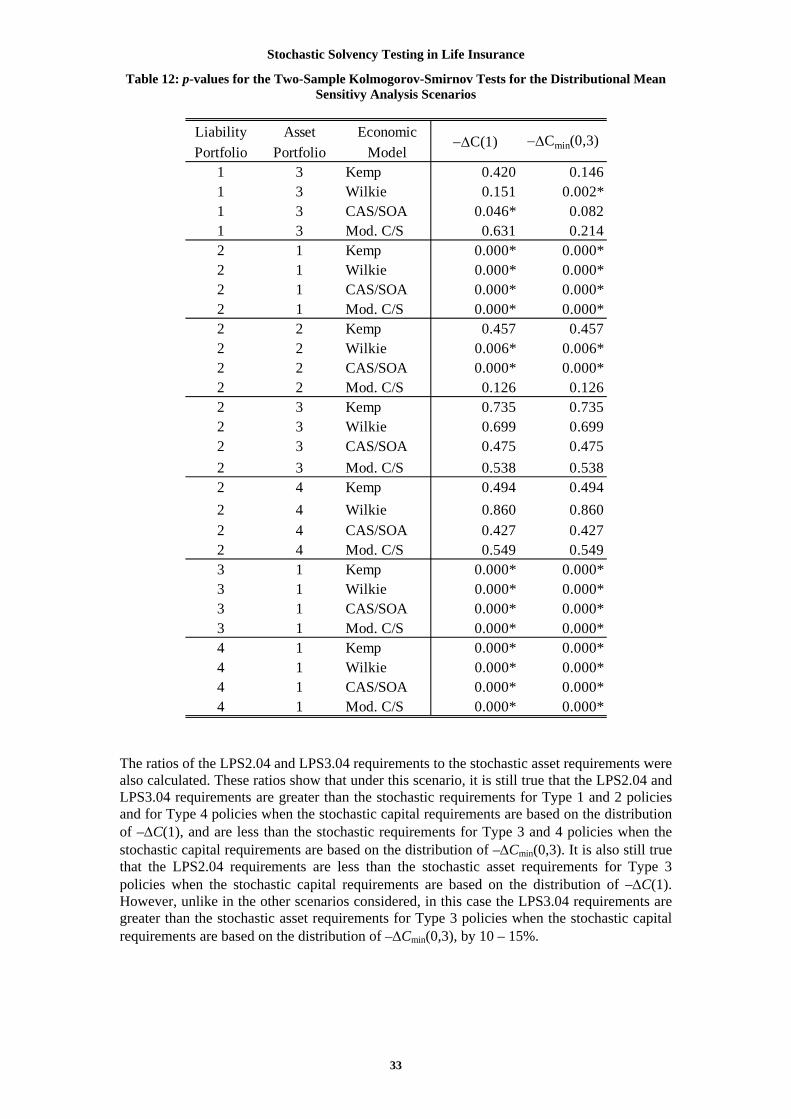
Stochastic Solvency Testing in Life Insurance
Table 12: p-values for the Two-Sample Kolmogorov-Smirnov Tests for the Distributional Mean Sensitivy Analysis Scenarios
Liability Asset EconomicPortfolio Portfolio Model
1 3 Kemp 0.420 0.1461 3 Wilkie 0.151 0.002*1 3 CAS/SOA 0.046* 0.0821 3 Mod. C/S 0.631 0.2142 1 Kemp 0.000* 0.000*2 1 Wilkie 0.000* 0.000*2 1 CAS/SOA 0.000* 0.000*2 1 Mod. C/S 0.000* 0.000*2 2 Kemp 0.457 0.4572 2 Wilkie 0.006* 0.006*2 2 CAS/SOA 0.000* 0.000*2 2 Mod. C/S 0.126 0.1262 3 Kemp 0.735 0.7352 3 Wilkie 0.699 0.6992 3 CAS/SOA 0.475 0.4752 3 Mod. C/S 0.538 0.5382 4 Kemp 0.494 0.4942 4 Wilkie 0.860 0.8602 4 CAS/SOA 0.427 0.4272 4 Mod. C/S 0.549 0.5493 1 Kemp 0.000* 0.000*3 1 Wilkie 0.000* 0.000*3 1 CAS/SOA 0.000* 0.000*3 1 Mod. C/S 0.000* 0.000*4 1 Kemp 0.000* 0.000*4 1 Wilkie 0.000* 0.000*4 1 CAS/SOA 0.000* 0.000*4 1 Mod. C/S 0.000* 0.000*
−ΔC(1) −ΔCmin(0,3)
The ratios of the LPS2.04 and LPS3.04 requirements to the stochastic asset requirements were also calculated. These ratios show that under this scenario, it is still true that the LPS2.04 and LPS3.04 requirements are greater than the stochastic requirements for Type 1 and 2 policies and for Type 4 policies when the stochastic capital requirements are based on the distribution of –ΔC(1), and are less than the stochastic requirements for Type 3 and 4 policies when the stochastic capital requirements are based on the distribution of –ΔCmin(0,3). It is also still true that the LPS2.04 requirements are less than the stochastic asset requirements for Type 3 policies when the stochastic capital requirements are based on the distribution of –ΔC(1). However, unlike in the other scenarios considered, in this case the LPS3.04 requirements are greater than the stochastic asset requirements for Type 3 policies when the stochastic capital requirements are based on the distribution of –ΔCmin(0,3), by 10 – 15%.
33
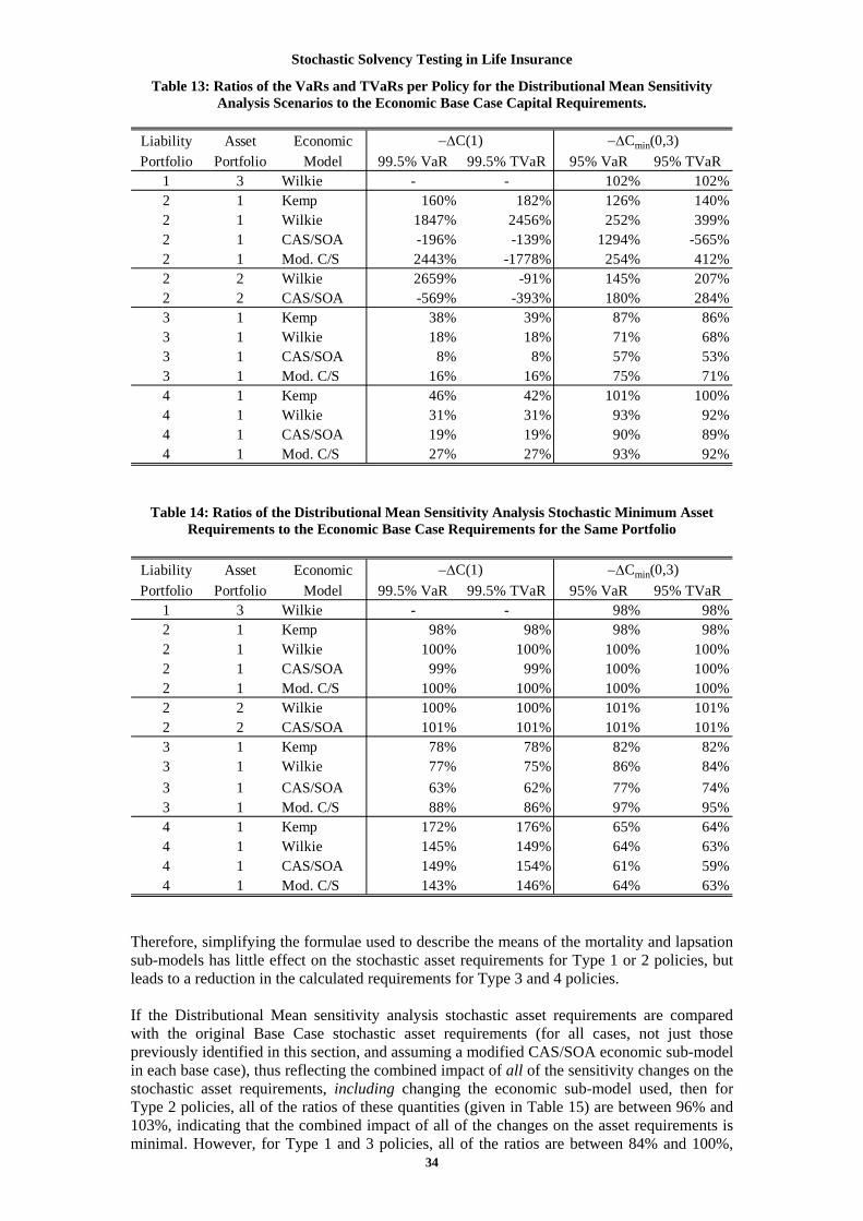
Stochastic Solvency Testing in Life Insurance
Table 13: Ratios of the VaRs and TVaRs per Policy for the Distributional Mean Sensitivity Analysis Scenarios to the Economic Base Case Capital Requirements.
Liability Asset EconomicPortfolio Portfolio Model 99.5% VaR 99.5% TVaR 95% VaR 95% TVaR
1 3 Wilkie - - 102% 102%2 1 Kemp 160% 182% 126% 140%2 1 Wilkie 1847% 2456% 252% 399%2 1 CAS/SOA -196% -139% 1294% -565%2 1 Mod. C/S 2443% -1778% 254% 412%2 2 Wilkie 2659% -91% 145% 207%2 2 CAS/SOA -569% -393% 180% 284%3 1 Kemp 38% 39% 87% 86%3 1 Wilkie 18% 18% 71% 68%3 1 CAS/SOA 8% 8% 57% 53%3 1 Mod. C/S 16% 16% 75% 71%4 1 Kemp 46% 42% 101% 100%4 1 Wilkie 31% 31% 93% 92%4 1 CAS/SOA 19% 19% 90% 89%4 1 Mod. C/S 27% 27% 93% 92%
−ΔC(1) −ΔCmin(0,3)
Table 14: Ratios of the Distributional Mean Sensitivity Analysis Stochastic Minimum Asset Requirements to the Economic Base Case Requirements for the Same Portfolio
Liability Asset EconomicPortfolio Portfolio Model 99.5% VaR 99.5% TVaR 95% VaR 95% TVaR
1 3 Wilkie - - 98% 98%2 1 Kemp 98% 98% 98% 98%2 1 Wilkie 100% 100% 100% 100%2 1 CAS/SOA 99% 99% 100% 100%2 1 Mod. C/S 100% 100% 100% 100%2 2 Wilkie 100% 100% 101% 101%2 2 CAS/SOA 101% 101% 101% 101%3 1 Kemp 78% 78% 82% 82%3 1 Wilkie 77% 75% 86% 84%3 1 CAS/SOA 63% 62% 77% 74%3 1 Mod. C/S 88% 86% 97% 95%4 1 Kemp 172% 176% 65% 64%4 1 Wilkie 145% 149% 64% 63%4 1 CAS/SOA 149% 154% 61% 59%4 1 Mod. C/S 143% 146% 64% 63%
−ΔC(1) −ΔCmin(0,3)
Therefore, simplifying the formulae used to describe the means of the mortality and lapsation sub-models has little effect on the stochastic asset requirements for Type 1 or 2 policies, but leads to a reduction in the calculated requirements for Type 3 and 4 policies.
34
If the Distributional Mean sensitivity analysis stochastic asset requirements are compared with the original Base Case stochastic asset requirements (for all cases, not just those previously identified in this section, and assuming a modified CAS/SOA economic sub-model in each base case), thus reflecting the combined impact of all of the sensitivity changes on the stochastic asset requirements, including changing the economic sub-model used, then for Type 2 policies, all of the ratios of these quantities (given in Table 15) are between 96% and 103%, indicating that the combined impact of all of the changes on the asset requirements is minimal. However, for Type 1 and 3 policies, all of the ratios are between 84% and 100%,

Stochastic Solvency Testing in Life Insurance
indicating a moderate decrease in the asset requirements in these cases, and for Type 4 policies, more substantial decreases in the asset requirements are suggested (note that, again, although some of the ratios are greater than 100%, these ratios indicate a decrease in the asset requirements, because they correspond to situations with negative asset requirements). In summary, the overall effect of all of the model changes made in the sensitivity analyses is either very small, for Type 2 policies, or for other policy types, the effect is to decrease the requirements, with the greatest percentage decreases being for Type 4 policies.
Table 15: Ratios of the Distributional Mean Sensitivity Analysis Stochastic Minimum Asset Requirements to the (Original) Base Case Requirements for the Same Portfolio
Liability Asset EconomicPortfolio Portfolio Model 99.5% VaR 99.5% TVaR 95% VaR 95% TVaR
1 3 Kemp 88% 86% 92% 88%1 3 Wilkie 88% 86% 99% 98%1 3 CAS/SOA 86% 84% 89% 86%1 3 Mod. C/S 86% 84% 89% 86%2 1 Kemp 100% 100% 100% 100%2 1 Wilkie 100% 100% 101% 100%2 1 CAS/SOA 100% 100% 100% 100%2 1 Mod. C/S 100% 100% 100% 100%2 2 Kemp 101% 101% 103% 102%2 2 Wilkie 100% 101% 101% 101%2 2 CAS/SOA 100% 100% 101% 101%2 2 Mod. C/S 101% 101% 103% 102%2 3 Kemp 99% 98% 101% 100%2 3 Wilkie 99% 98% 101% 100%2 3 CAS/SOA 99% 98% 101% 100%2 3 Mod. C/S 99% 98% 101% 100%2 4 Kemp 97% 96% 100% 99%2 4 Wilkie 97% 96% 100% 99%2 4 CAS/SOA 97% 96% 100% 99%2 4 Mod. C/S 97% 96% 100% 99%3 1 Kemp 88% 85% 97% 95%3 1 Wilkie 91% 89% 99% 97%3 1 CAS/SOA 88% 86% 96% 94%3 1 Mod. C/S 88% 86% 97% 95%4 1 Kemp 146% 150% 64% 63%4 1 Wilkie 144% 147% 64% 63%4 1 CAS/SOA 143% 147% 64% 63%4 1 Mod. C/S 143% 146% 64% 63%
−ΔC(1) −ΔCmin(0,3)
7 Conclusion
7.1 Summary of Results In this paper we presented a stochastic solvency testing model, originally developed by Hayes (2008), in the context of the Australian Life Insurance environment, in anticipation that APRA will ultimately require Australian Life Insurers to calculate their solvency capital requirements using stochastic methods. The model is a simulation model which comprises three stochastic sub-models used to describe the economic environment and the mortality and lapsation experience of the portfolio of policies under consideration: (i) a modified CAS/SOA
35

Stochastic Solvency Testing in Life Insurance
36
economic sub-model; (ii) a Poisson or negative binomial (NB1) distribution as the mortality sub-model; and (iii) a normal-Poisson lapsation sub-model. Allowance was made for observed dependency relationships between short-term interest rates and mortality, and between economic variables and lapsation rates, throughout. The model was then used to conduct tests to determine the adequacy of Australia’s current deterministic solvency capital requirements. Results show that for Type 1 and 2 policies, the LPS2.04 solvency capital requirement and the LPS3.04 capital adequacy capital requirement are much greater than the 99.5% VaR and TVaR values and 95% VaR and TVaR values. However, for Type 4 policies, the LPS2.04 and LPS3.04 capital requirements are greater than the 99.5% VaR and TVaR values of –ΔC(1), and much less than the 95% VaR and TVaR values of –ΔCmin(0,3); while for Type 3 policies, the LPS2.04 and LPS3.04 capital requirements are generally less than all of the stochastic capital requirements. Similarly, the LPS2.04 and LPS3.04 requirements are generally greater than the stochastic asset requirements, with the exception of the Type 3 policy cases, and the Type 4 policy cases when solvency is considered over a three year time horizon, in which case the opposite is true. Tests conducted in Hayes (2008) show that the stochastic solvency testing model described in this paper is the “most suitable” model (out of a specified selection of models) for use by an Australian Life Insurer. However, sensitivity analysis conducted, in this paper, to determine the impact on the results of using alternative sub-models to the “best” sub-models (including ignoring the dependency relationships previously mentioned and simplifying the formulae used to calculate the model means) show that using a Poisson distribution in place of the NB1 sub-model has no significant effect on the overall results. They also show that, although using a Poisson distribution in place of the normal-Poisson lapsation sub-model or ignoring the observed dependency relationships does, in some cases, have a significant effect on the distributions of the simulation outputs, these changes have virtually no effect on the minimum assets that the insurer must hold under each of the stochastic solvency criteria. On the other hand, if an alternative economic sub-model is used, or if the simplified mean structure described in Section 5.3 is used, these changes not only have a significant impact on the simulation output distributions, but also impact the results of the (stochastic) minimum asset requirement calculations for some policy types. If either the Kemp, Wilkie or CAS/SOA economic model is used in place of the modified CAS/SOA model, this leads to higher total asset requirements for Type 3 policies, while if the simplified mean structure is used, this leads to lower minimum asset requirements for Type 3 and 4 policies. The overall effect on the minimum asset requirements of making all of these changes together is to lower the requirements for Type 1, 3 and 4 policies, with little effect on the requirements for Type 2 policies.
7.2 Implications According to Karp (2002), the current Australian Life Insurance solvency requirement is set at a 95% sufficiency level over a three year time horizon, while many other insurance regulators throughout the world set their solvency requirements at a 99.5% sufficiency level over a one year time horizon. The results of this paper demonstrate that, for a typical Australian Life Insurer, although both of these criteria are more than met by the deterministic LPS2.04 and LPS3.04 requirements, if a portfolio of either Type 1 or Type 2 policies is held, the LPS2.04 and LPS3.04 requirements for a typical portfolio of Type 3 policies do not meet either of the above criteria, and although the LPS2.04 and LPS3.04 requirements for a typical portfolio of Type 4 policies meet the 99.5% sufficiency level over a one year time horizon, they do not meet the 95% sufficiency level over a three year time horizon, claimed by APRA. The implications of these results are that the current Australian Life Insurance requirements do not provide the same level of protection against insolvency for all insurers, and, especially when solvency is considered over a three year time horizon, provide little protection against insolvency for insurers who primarily write Type 3 and 4 insurance business, that is,
Stochastic Solvency Testing in Life Insurance
37
“mortality risk” insurance policies. Despite this, few solvency problems have resulted from the current solvency and capital adequacy requirements. According to Davis (2004), in the period from 1901 to 200311, only “11 (Australian) Life Insurers entered liquidation, with the majority of these occurring during the late 1920's and early 1930's, and one in 1954. … The most recent cases of (Life Insurer) failure are that of Occidental Life and Regal Life”, which occurred in 1990. This low frequency of problems is probably because most insurers hold diverse liability portfolios not primarily comprised of Type 3 and 4 policies (so there would be some offsetting of the capital requirements between the different policy types); it is common practice for insurers to hold more than the bare minimum amount of capital; and no catastrophic events (from a Life Insurer's point of view), such as an influenza pandemic, have occurred in Australia in recent years. Given these issues, however, we suggest that it would be advisable for APRA to amend the existing Life Insurance solvency requirements either to increase the deterministic requirements for portfolios containing Type 3 or 4 policies, or to move from a deterministic solvency capital calculation regime to a stochastic regime. The advantage of the former approach is that it is likely to be the cheaper of the two to implement, as there are cost implications for APRA of radically rewriting the existing solvency and capital adequacy standards, and for insurers of implementing more complex solvency testing models. Nevertheless, we suggest that the latter approach is preferable, since it would promote the desirable outcome of specifying consistent capital requirements between insurers, with respect to sufficiency levels, and furthermore, is in line with the current trends in insurance regulation in the developed world. If APRA were to require Life Insurers to calculate their solvency capital requirements on a stochastic basis, then some guidance should be provided to insurers as to which components should be included in their solvency testing model, as differences in the model can have a significant impact on the calculated capital requirement. On the basis of our investigation, it appears to be unnecessary for insurers to be required to allow for either mortality or lapsation over-dispersion, or for dependency relationships between mortality rates, lapsation rates and the economy, in the model, as, ultimately, these had little effect on the overall asset requirements of the insurer in our study. However, as the choice of economic sub-model and the level of complexity of the mean mortality rate and lapsation rate assumptions do significantly impact the calculated asset requirements for some policy types, in order to ensure consistency between insurers, it is recommended that APRA select a single economic sub-model for use in all solvency calculations and provide guidelines for setting the sub-model means.
7.3 Limitations and Further Research As with any research, the scope of the research conducted in this paper was limited by the availability of data. A number of the assumptions made in this paper, particularly in Section 5.2, were based on evidence obtained from publicly available data, such as insurer annual reports, which is not as detailed as the private data that is available to insurers (for confidentiality reasons, this information could not be obtained, with the exception of the data sets described in Section 3). The availability of more detailed information would lead to an increase in the level of accuracy of the assumptions underlying the solvency testing model, and hence, an increase in the accuracy of the results. In Section 5.2.1, it was pointed out that the results of the analysis carried out in this paper may potentially change, depending on the composition of the insurance portfolio under consideration. Subsequently, seven model portfolios were constructed for investigation purposes, reflecting a range of different product types and investment strategies. However, these are not the only possible portfolios. Investigating different business mixes (for example,
11 The current Life Insurance solvency and capital adequacy requirements were first introduced in 1995.
Stochastic Solvency Testing in Life Insurance
38
portfolios containing more than one policy type) or portfolios containing policies of different sizes would provide additional insight into the adequacy of the existing solvency requirements. Further, in this paper only investment (Type 1 and Type 2 policies) and mortality risk (Type 3 and 4 policies) Life Insurance products were considered, not retirement income products (such as life annuities or allocated annuities) nor disability/morbidity risk products (such as disability income insurance or trauma insurance), in spite of the fact that these product types represent a significant proportion of the total premium income received by Australian Life Insurers each year. This was, again, due to the fact that data relating to these products could not be obtained. Consequently, repeating the tests carried out in this paper for the unconsidered Life Insurance product types could form a basis for useful further research. Finally, all assumptions made in this paper are based on the economic and regulatory conditions that Australia has experienced in recent years and on the recent experience of Australian Life Insurers. However, the economy, regulations and insurer experience are constantly changing, and if the investigations performed in this paper were repeated using data relating to a different period of time, it is possible that different results would be observed and alternative conclusions reached. References Ahlgrim, K., D’Arcy, S., & Gorvett, R., 2004, Modeling of Economic Series Coordinated with Interest Rate Scenarios, Research report, Casualty Actuarial Society and Society of Actuaries. Albert, F., & Bragg, J., 1996, Mortality Rates as a Function of Lapse Rates, Research report, Society of Actuaries. Alho, J., 2005, ‘Remarks on the use of probabilities in demography and forecasting’, in N. Keilman (Ed.), Perspectives on Mortality Forecasting II: Probabilistic Forecasting, pp. 27 – 38, Swedish Social Insurance Agency, Stockholm. APRA, 2007, APRA Life Office Market Report June 2007. BIS, 2006, Basel II: International Convergence of Capital Measurement and Capital Standards: A Revised Framework – Comprehensive Version. Cameron, A., and Trivedi, P., 1986, ‘Econometric models based on count data: Comparisons and applications of some estimators’, Journal of Applied Econometrics, 1, pp. 29 – 53. CEA, 2006, Solvency II: Cost of Capital, Position Paper 291, Comité Européen des Assurances. CEA & Mercer Oliver Wyman, 2005, Solvency Assessment Models Compared, Research report, Comité Européen des Assurances. Choice, 2007, Buying Guide: Managed Funds, Downloaded from http://www.choice.com.au on 28/03/08. Davis, K., 2004, Study of Financial System Guarantees, Government report, Commonwealth of Australia. Daykin, C., Pentikäinen, T., & Pesonen, M., 1994, Practical Risk Theory for Actuaries, Chapman and Hall, London. EU, 2007, Solvency II: Frequently Asked Questions (FAQs), Press release downloaded from http://europa.eu on 31/08/07.

Stochastic Solvency Testing in Life Insurance
39
FOPI, 2004, White Paper on the Swiss Solvency Test, White paper, Swiss Federal Office of Private Insurance. FOPI, 2006, The Swiss Experience with Market Consistent Technical Provisions – the Cost of Capital Approach, Research paper, Swiss Federal Office of Private Insurance. Hayes, G., 2008, Stochastic Solvency Testing in Life Insurance, Ph. D. thesis, The Australian National University. IAA, 2004, A Global Framework for Insurer Solvency Assessment, Research report, IAA Insurer Solvency Assessment Working Party, International Actuarial Association. IAAust Mortality Committee, 2001, Mortality Investigation IA 95-97 M and F: Graduated Mortality Tables, Institute of Actuaries of Australia. Jones, B., 1998, ‘A model for analysing the impact of selective lapsation on mortality’, North American Actuarial Journal, 2, pp. 79 – 86. J.P. Morgan/Reuters, 1996, RiskMetrics – Technical Document, 4th ed., J.P. Morgan/Reuters, New York. Karp, T., 2002, ‘Dynamic solvency testing models’, Presented to the IAIS Annual Conference, Chile. Kaufmann, R., Gadmer, A., & Klett, R., 2001, ‘Introduction to dynamic financial analysis’, ASTIN Bulletin, 31, pp. 213 – 249. Lambert, D., 1992, ‘Zero-inflated Poisson regression, with an application to defects in manufacturing’, Technometrics, 34, pp. 1 – 14. Lee, P., 2000, ‘A general framework for stochastic investigations of mortality and investment risks’, Presented at Wilkiefest, Heriot-Watt University. Mullahy, J., 1986, ‘Specification and testing of some modified count data models’, Journal of Econometrics, 33, pp. 341 – 365. Rabe-Hesketh, S., & Skrondal, A., 2005, Multilevel and Longitudinal Modeling, Stata Press, Texas. Sandström, A., 2006, Solvency: Models, Assessment and Regulation, Chapman and Hall/CRC, Florida. Smith, A., 1995, ‘Workshop on stochastic asset models’, Presented to the Institute of Actuaries General Insurance Convention, Bournemouth. Smith, A., 1996, ‘How actuaries can use financial economics’, British Actuarial Journal, 2, pp. 1057 – 1174. Tsai, C., Kuo, W., & Chen, W., 2001, ‘Early surrender and the distribution of policy reserves’, Insurance: Mathematics and Economics, 31, pp. 429 – 445. Valdez, E., 2001, ‘Bivariate analysis of survivorship and persistency’, Insurance: Mathematics and Economics, 29, pp. 357 – 373. Wilkie, A., 1986, ‘A stochastic investment model for actuarial use’, Transactions of the Faculty of Actuaries, 39, pp. 341 – 403.

Stochastic Solvency Testing in Life Insurance
40
Wilkie, A., 1995, ‘More on a stochastic asset model for actuarial use’, British Actuarial Journal, 1, pp. 777 – 964.