stock options compensation as a commitment … · stock options compensation as a commitment...
TRANSCRIPT

Stock Options Compensation as a CommitmentMechanism in Oligopoly Competition
David Hao Zhang
April 17, 2013
Submitted to theDepartment of Economics
of Amherst Collegein partial fulfillment of the requirements
for the degree ofBachelor of Arts with honors
Faculty Advisor: Professor Jun Ishii

Acknowledgements
Above all, I want to thank Professor Ishii in the Economics Department at
Amherst College. He has been extremely supportive over my thesis writing
process. He guided me through much of the literature on industrial organi-
zation, and gave me advice on my direction of research. He also edited my
thesis drafts thoroughly. I had a fantastic time working with him, and could
not have completed this project without him.
I would also like to thank Professor Nicholson for introducing me to the beauty
of economic theory in Advanced Microecnomics (the first economics course I
took at Amherst), and for being so patient with me as I explored my crazy
ideas. He is the reason I majored in economics, and his perspectives on eco-
nomic modelling and the contractual nature of the firm continue to influence
my everyday thinking. Also, I would like to thank Professor Woglom for
introducing me to the Economics of Finance, which greatly influenced the
theoretical approach of this thesis. His Advanced Macroeconomics class is
perhaps one of the most relevant classes I have taken. I would also like to
thank Professor Reyes for teaching the fun first semester thesis course, which
helped me select a thesis topic and introduced me to economics research, and
Professor Kingston, for teaching a fantastic course on Game Theory. Finally,
I would like to thank the entire Economics Department at Amherst College
for teaching me the skills and ways of thinking that made this thesis possible,
and for being so supportive of the thesis writing experience.
i

I would also like to thank my friends and colleagues at Amherst College who
has given me the strength to complete my thesis. In particular, I’d like to
thank Ben Pullman, who helped me with my presentation and supplied me
with homemade coffee, and Zach Bleemer, who served as a source of comfort
by letting me know that one other dual-thesis writer is out there. I would like
to thank my girlfriend, Juean Chen from Rice University, for supporting me
in the data gathering process and for listening to me going on and on about
half-baked ideas.
Finally, I would like to thank my family for making it all possible. Thank you
mom and dad. I love you.
ii

Abstract
Stock options have become an important component of contemporary manage-
rial compensation. According to Frydman and Jenter (2010), in 2005 around
37% of CEO compensation was in the form of stock options. It is widely ac-
knowledged that stock options compensation makes managers more willing to
take risks. In this paper, I show how a commitment to risk taking through
stock options compensation can lead to a strategic advantage in oligopolistic
competition. I develop a two period model whereby in the first period share-
holders choose a compensation structure for their managers and in the second
period managers choose production under Cournot competition with uncertain
demand or marginal cost. I show that in equilibrium shareholders will struc-
ture managerial compensation and use stock options to make their managers
risk-taking. The idea that shareholders could incentivise excessive risk-taking
behavior in their managers has important welfare implications. I also investi-
gate a testable implication of my model: that the equilibrium levels of options
compensation is positively related to the market power of the firms. Using
options compensation data from Capital IQ and industry concentration as a
proxy for market power, I show that as predicted the level of options compen-
sation is positively related to the level of industry concentration (p < 0.001).
iii

Contents
1 Introduction 1
2 Literature Review 4
3 Model 10
3.1 Model setup . . . . . . . . . . . . . . . . . . . . . . . . . . . . 10
3.2 General model . . . . . . . . . . . . . . . . . . . . . . . . . . . 12
3.3 Numerical Illustration . . . . . . . . . . . . . . . . . . . . . . 18
3.4 Graphical Illustration . . . . . . . . . . . . . . . . . . . . . . . 20
3.5 Consequences for social welfare . . . . . . . . . . . . . . . . . 21
4 Empirical Exploration 22
4.1 Introduction . . . . . . . . . . . . . . . . . . . . . . . . . . . . 22
4.2 Identification Method . . . . . . . . . . . . . . . . . . . . . . . 24
4.3 Results . . . . . . . . . . . . . . . . . . . . . . . . . . . . . . . 25
5 Comment on innovation 30
6 Conclusion 31
Bibliography 33
7 Appendix 37
7.1 Detailed derivation for the basic model . . . . . . . . . . . . . 37
7.2 Numerical Example . . . . . . . . . . . . . . . . . . . . . . . . 40
7.3 Welfare implications . . . . . . . . . . . . . . . . . . . . . . . 44
iv

7.4 Regression without fixed effects . . . . . . . . . . . . . . . . . 47
v

1 Introduction
Stock options are an important component of contemporary managerial com-
pensation. In 2005, around 37% of CEO compensation was in the form of stock
options (Frydman and Jenter, 2010). Since the 1980s, economists primarily
understood stock options compensation as an instrument by which risk neu-
tral shareholders (the principals) aligned the incentives of risk averse managers
(the agents) in the presence of asymmetric information.
However, the focus on the alignment of incentives misses an important strategic
dimension to the principal agent problem. The principal agent problem is
characterized by an existence of an agent who has to be incentivized to act
in the best interests of the principal. The presence of agents who acts on the
principals’ behalf without necessarily conforming to the principals’ interests
give the principals an opportunity to credibly commit to a set of strategies
that may be different from what the principals would choose themselves.
For example, the shareholders may be expected profit maximizing, but if they
incentivise their managers to be risk taking, they can credibly commit to a
risk taking set of strategies. If the principals engage in strategic interactions
with other players, the ability to make such credible commitments enables the
principals to earn a strategic advantage similar to that of the first mover in the
Stackelberg competition model (Heinrich von Stackelberg, 1934). As such, my
thesis is based on an analysis of principal agent relationships whereby agent
compensation setting incorporates the commitment value of various compen-
1

sation schemes.
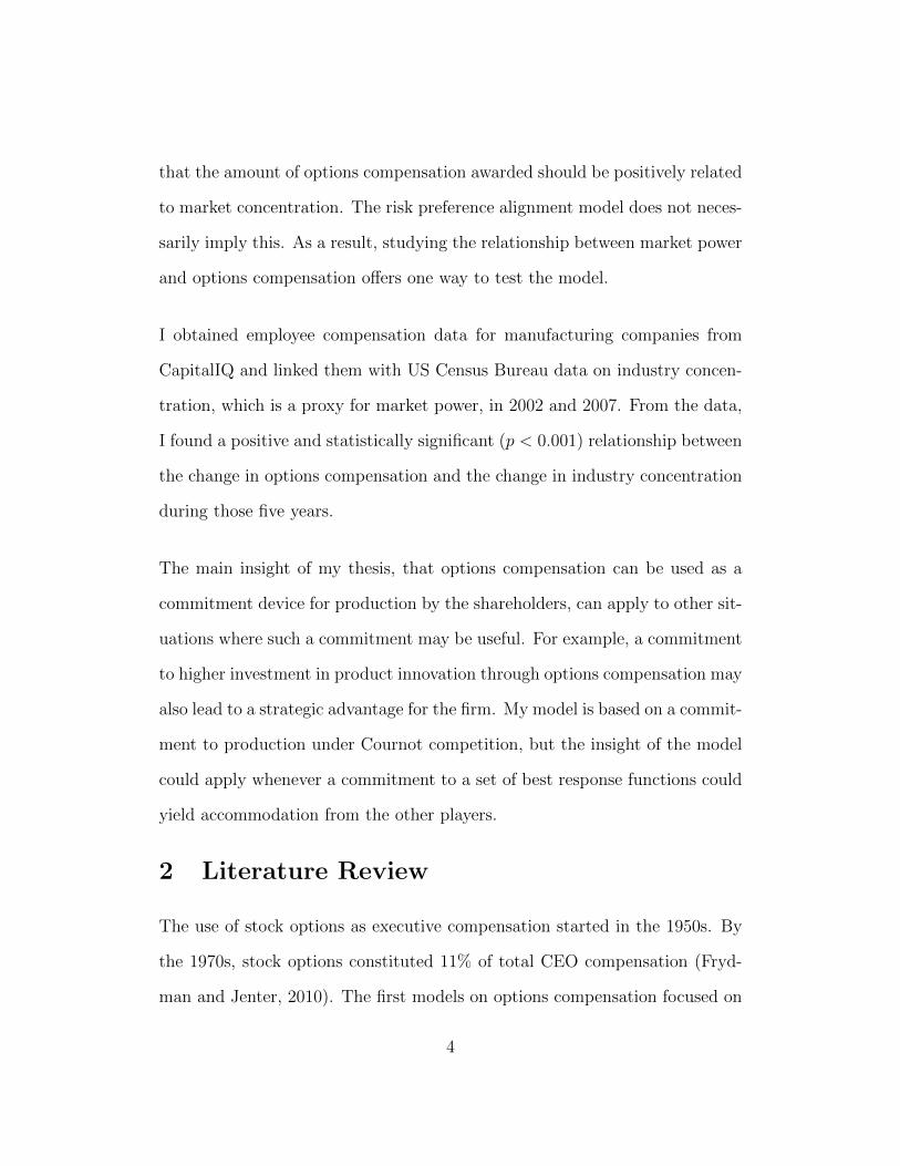
Figure 1: A flow chart showing how the agent’s incentives can be a usefulcommitment device for the principal
My thesis shows how stock options awards can lead to a strategic advantage
by allowing shareholders to commit to a risk-taking set of strategies. The
awarding of stock options leads to greater management risk taking because
stock options enable managers to enjoy the potential upside gain (a rise in
stock value) while protected from the downside risk (a fall in stock value) of
their decisions. By credibly incentivising managers to take risks through op-
tions compensation, firms can commit to a more aggressive management style.
With uncertain returns on production due to demand and cost uncertainty,
managers incentivised to be risk seeking face incentives to overproduce in or-
2

der to increase the volatility of the returns of the firm. The public knowledge
that a firm has a credible commitment to overproduce may force the other
firms to scale back their own planned production to avoid flooding the mar-
ket. As a result, in equilibrium, all firms adopt stock options compensation
and incentivise their managers to be risk taking in order to avoid ending up
as a disadvantaged Stackelberg follower.
The insight I propose can be demonstrated within a two stage Cournot oligopoly
model. In the first stage, shareholders choose the compensation structure for
managers. In the second stage, managers choose production under Cournot
oligopoly with uncertain demand or cost. This approach differs from the in-
centive alignment model traditionally used to explain stock options compen-
sation in that it implies that executive compensation will incentivise managers
to be risk taking rather than risk neutral. Dong, Wang, and Xie (2010) gives
empirical evidence that stock options compensation for managers is associ-
ated with financing decisions that leave firms over-leveraged, suggesting that
shareholders do incentivise risk taking (instead of incentive alignment and risk
neutrality) in managers.
My model implies that the equilibrium executive compensation structure is
related to the extent of market power available to the firms in an industry. It
is less relevant when the market approaches perfect competition where indi-
vidual firm decisions do not influence the decisions of other firms. If firms do
not have market power, committing to a certain set of actions can yield no
response from other firms and hence no competitive advantage. This means
3
that the amount of options compensation awarded should be positively related
to market concentration. The risk preference alignment model does not neces-
sarily imply this. As a result, studying the relationship between market power
and options compensation offers one way to test the model.
I obtained employee compensation data for manufacturing companies from
CapitalIQ and linked them with US Census Bureau data on industry concen-
tration, which is a proxy for market power, in 2002 and 2007. From the data,
I found a positive and statistically significant (p < 0.001) relationship between
the change in options compensation and the change in industry concentration
during those five years.
The main insight of my thesis, that options compensation can be used as a
commitment device for production by the shareholders, can apply to other sit-
uations where such a commitment may be useful. For example, a commitment
to higher investment in product innovation through options compensation may
also lead to a strategic advantage for the firm. My model is based on a commit-
ment to production under Cournot competition, but the insight of the model
could apply whenever a commitment to a set of best response functions could
yield accommodation from the other players.
2 Literature Review
The use of stock options as executive compensation started in the 1950s. By
the 1970s, stock options constituted 11% of total CEO compensation (Fryd-
man and Jenter, 2010). The first models on options compensation focused on
4

the usefulness of stock options compensation in addressing the principal-agent
problem between risk averse managers and risk neutral shareholders. They in-
clude Haugen and Senbet (1981), Smith and Stulz (1985), and Greenwald and
Stiglitz (1990), and are now recognized as standard explanations for options
compensation.
In these models, the managers and the shareholders have conflicting interests
regarding risk. While shareholders can eliminate idiosyncratic risk through di-
versification, managers cannot due to their specific human capital investment
that are tied to the firm. As a result, shareholders are more likely to prefer a
risk neutral and expected profit maximizing style of decision making than the
managers. Given some information asymmetry between managers and share-
holders, managers who are risk averse may be able to mask their risk averse
managing of the firm. The inclusion of options in the managers’ compensation
presumably makes managers more willing to take risks and lead to decisions
that are more aligned with shareholder interests. There are many empirical
studies linking options compensation with increased risk taking, including Ra-
jgopal and Shevlin (2002), Coles, Naveen, and Lalitha (2006), and Gormley,
Matsa, and Milbourn (2012).
A number of extensions has been made to the theory of options compensation
since the 1980s. Zhang (1998) expanded on the mainstream principal-agent
model to include the observation that shareholder vigilance would lead to
shareholder concentration and risk aversion in firm behavior as long as infor-
mation was costly to obtain. The awarding of risk rewarding compensation
5

to managers, then, is better able to induce risk-neutral decision making than
shareholder vigilance. Other models explore the usefulness of options on em-
ployee sorting in terms of the labor economics associated with hiring capable
employees. Lazear (2004) derives a model whereby employee skill is assumed
to be known to the employees but unknown to the employers (thus leading to
asymmetric information in skill levels), and derives a model where pay tied to
firm performance would attract able employees to work at the firm. Options
compensation for managers, then, would attract capable managers.
Partly due to the success of these models in demonstrating the usefulness of
that options compensation, provisions in the Omnibus Budget Reconciliation
Act of 1993 (OBRA 1993) encouraged options based compensation by ex-
empting it from the $1 million cap on the deductibility of employment based
compensation. Hanlon and Shevlin (2002) noted that the use of employee
stock options reduced the amount of taxes owed by the firm by allowing firms
to circumvent the cap on the deductibility of employee compensation. Another
explanation of options compensation from the accounting perspective comes
from Core, Guay, and Larcker (2003). Core, Guay, and Larcker explained that
the Generally Accepted Accounting Principles (GAAP) used in financial ac-
counting allow the expenses of awarding options compensation to be hidden
from income statements. Options compensation can be valued by the differ-
ence between the exercise price and the stock price of the firm under GAAP.
Since options are usually awarded with a strike price equal to the current stock
price of the firm (ie. with a difference of zero), the expense of options com-
6

Figure 2: A chart showing the importance of options compensation as a com-ponent of CEO compensation in S&P500 firms by Frydman and Jenter (2010)
pensation is hidden from income statements. Options compensation increased
to 32% of total CEO compensation in the 1990s and to 37% in the early 2000s
(Frydman and Jenter, 2010).
The common theme of imperfect information models is that they assume some
sort of asymmetric information between the employers (the principals) and the
employees (the agents). They introduce options compensation as a way to work
around the information constraints by aligning the incentives of managers and
shareholders. The theory of asymmetric information is insightful and expan-
sive, and its pioneers are awarded well deserved Nobel Prizes in economics
7

in 2001. Nevertheless, asymmetric information may not be necessary to ex-
plain options compensation, and the alignment of the shareholder/manager
decision making process may not lead to the profit maximizing managerial
compensation structure.
My thesis explains how options compensation can be used as a commitment
device in oligopoly competition, and proposes an alternative mechanism by
which options are awarded. The intuition for my model is similar to that
in Allaz and Vila (1993). Allaz and Vila (1993) modeled how firms could
use the forward market in stage one to commit to production in stage two,
hence gaining a competitive advantage as a first-mover. In a simultaneous
game, Allaz and Vila (1993) showed that all firms would participate in forward
markets even though by doing so, the firms pre-commit to greater production
and drive down prices. As such, the paper explains the existence of forward
markets under perfect information by pointing out the strategic element of
participating in forward markets. I show that there is a similar strategic
element in options compensation: awarding options compensation is a way of
pre-committing to risk taking, which in a world of uncertain demand and cost
means a pre-commitment to production.
The idea that firms would commit to aggressive strategies through managerial
compensation was explored in Fershtman (1985), Fershtman and Judd (1987)
and Sklivas (1987), which are sometimes referred to as the FJS models. Similar
to my model, the FJS models are two stage models where shareholders set
compensation in the first stage and managers set production in the second
8

stage. Their models showed that shareholders who design a compensation
package based on profits and revenue will choose a compensation schedule that
leads to managers aggressively setting production beyond the Cournot Nash
equilibrium. Instead of depending on a revenue based compensation schedule
as a pre-commitment, my model shows how risk based compensation (options
compensation) can also be used by shareholders to commit their managers to
be aggressive.
Reitman (1993) also explored options compensation as a commitment mecha-
nism under the the FJS model. However, he treated options as a discontinuous
pay-off schedule based on profits that are revealed immediately when produc-
tion is set, and as a result did not incorporate the element of risk-taking into
his model. In my model, managers set production under demand or cost un-
certainty and maximize their expected utility based on the expected payoff
of their options. Unlike the Reitman (1993) model, my model incorporates
uncertainty and risk-taking behavior. Because one of the most cited rationale
for the use of stock options is to make managers more risk-taking, my model
uses a more complete characterization of options compensation than the one
Reitman (1993) used.
The existence of risk taking firms driven by managerial stock options is em-
pirically examined by Dong, Wang, and Xie (2010). Dong, Wang, and Xie
(2010) showed that stock options compensation for managers is associated
with financing decisions that leaves the firm over-leveraged, suggesting that
stock options compensation can indeed lead to excessive risk taking in firms
9

(and not simply risk neutrality, as the principal-agent shareholder manager
incentive alignment model would suggest).
3 Model
3.1 Model setup
I use a two period model with two sets of players, shareholders and managers,
to illustrate the strategic opportunity embedded in options compensation. In
this model, shareholders (principals) first choose a type of compensation for the
the managers (agents), and the managers then act on the shareholders’ behalf
given some uncertainty. I will show that through incentivising the managers
to be risk taking, shareholders can credibly commit to higher production and
behave as a first mover in an otherwise simultaneous Cournot game. Therefore,
in equilibrium, shareholders will structure managerial compensation so as to
make their managers risk taking. 1
I will first prove the result generally, then use a specific example to illustrate
the model more concretely. I will use the following notation in both the general
model and the specific example:
(x, y), indices for firm x and y
(qx, qy), the level of production set by managers in firm x and y
p, the price of the goods
c, the marginal cost of the goods
1And stock options compensation is a risk-inducing compensation scheme (with sometheoretical exceptions outlined in Ross, 2004 that is addressed in the appendix) that share-holders can use to make their managers risk taking.
10

ε, the uncertainty in either price or cost
σε, the standard deviation of the uncertainty in price or cost
π, the profit from production
σπ, the uncertainty in profit, as a standard deviation
f(π), a function relating the compensation awarded to managers to the profits
of the firm
E(), var(), the expected value and the variance
U(f), the utility function of the manager
U∗(E(π), σπ), the expected utility of the manager expressed as a function of
the expected value and the variance of the profits
I will assume that there exists either demand or cost uncertainty in the market
place, that shareholders are expected profit maximizing, and that the firms
engage in Cournot competition with linear demand and constant marginal cost
(such that p = a− qx− qy, and π = pq− cq = (p− c)q = (E(p)−E(c) + ε)q =
E(p)−E(c))q+εq). I will also assume that price or cost uncertainty, ε, follows
a distribution that is characterizable by the first two moments (such as the
Gaussian distribution). Under these assumptions, shareholders would design
executive compensation to induce a positive level of risk taking behavior from
the managers.
The manager of firm x sets the production qx to maximize expected utility of
the compensation f(πx):
maxqxE(U(f(πx))) (1)
11

Given the assumption that ε follows a distribution that is characterizable by
the first two moments, we can express managers’ expected utility in terms of
the mean (the first moment) and the variance (the second moment) of the
profits (Pennacchi, 2008, Ch. 2, which noted that E(U(π)) = U(E(π)) +
12var(π)U (2)(E(π)) + 1
8var(π)2U (4)(E(π) + ...)). As such, the managers’ incen-
tive function can be written as: maxqE(U(π)) = U∗(E(π), σπ).
Since shareholders could diversify away idiosyncratic risks, they are assumed
to be expected profit maximizing. As a result, shareholder of firm x’s incen-
tive is to structure management compensation f such that expected profit is
maximized:
maxfE(π) = E(p)q − E(c)q (2)
I set up the game so that shareholders choose executive compensation f(π)
with the understanding that managers choose qx in order to maximize the
expected utility from f(π). I will solve the game through backward induction:
I will first look at the equilibrium quantities and profits of managers playing a
Cournot game for a given f(π), and then explore how shareholders would set
f(π) with an understanding of the resulting equilibrium quantities.
3.2 General model
In this section I develop the key lemmas underlying my proposed insight on
the strategic value of options compensation. As such, I will be as general
as possible, and will only assume that managers have monotone increasing
12

and differentiable utility U(f) and that executive compensation f(π) is also
monotone increasing and differentiable, in the tradition of Ross (2004).
Lemma 3.1. The best response function of the managers can be expressed as
∂E(π)∂q
+ b(q) = 0, where b(q) takes the sign of ∂E(U)∂σπ
.
Proof. By first order condition for maximization:
dE(U(π))
dq≡ dU∗
dq=
∂U∗
∂E(π)
∂E(π)
∂q+∂U∗
∂σπ
∂σπ∂q
= 0
Dividing both sides by ∂U∗
∂E(π)yields:
∂E(π)
∂q+∂U∗
∂σπ
∂σπ∂q
∂U∗
∂E(π)
= 0
This can be expressed as:
∂E(π)
∂q+ b(q) = 0 (3)
where b(q) = ∂U∗
∂σπ
∂σπ∂q∂U∗∂E(π)
σπ = qσε, and therefore ∂σπ∂q
> 0. Furthermore, by the monotonic increasing
nature of f(π) and U(f), U(f(π)) is monotonically increasing in π and hence
∂U∗
∂E(π)> 0. As such, b(q) takes the sign of ∂U∗
∂σπ, or ∂E(U)
∂σπ.
Given this best response function, we are now able to find the Cournot Nash
equilibrium quantities chosen by managers in the second period for a given
13

utility function U(π). We can then determine whether shareholders would in-
centivise managers to be risk averse or risk taking through backward induction.
More specifically, we would investigate whether shareholders would incentivise
∂E(U)∂σπ
to be positive or negative. If ∂E(U)∂σπ
is greater than zero, the manager
can be said to be risk taking. If ∂E(U)∂σπ
is negative, the manager can be said
to be risk averse. Note that ∂E(U)∂σπ
= ∂E(U)∂f
∂f∂σπ
, which takes the sign of ∂f∂σπ
.
Hence, incentives for managers to be risk taking or risk averse are determined
by how their compensation f is affected by the variance of the profits ∂f∂σπ
.
Since stock options increase in value as the variance in profits increases, stock
options can be used to induce a risk taking behavior from the managers by
making ∂f∂σπ
> 0.
Lemma 3.2. Under Cournot oligopoly with two symmetric players, share-
holders would simultaneously set executive compensation structure such that
the managers would be incentivised to be risk taking. That is, both managers
will have ∂E(U)∂σπ
> 0.
Proof. First, the best response function for the managers of firm x and firm y
can be obtained by solving out the condition in Lemma 3.1:
qx =1
2(a− qy − E(c) + bx(qx)) (4)
qy =1
2(a− qx − E(c) + by(qy)) (5)
14

Solving these equations leads to the Cournot Nash equilibrium quantities:
qx =1
3(a− E(c) + 2bx − by) (6)
qy =1
3(a− E(c) + 2by − bx) (7)
Shareholders would choose an executive compensation structure f so as to
maximize firm profits under the equilibrium quantities qx and qy.
maxfE(π) = E(p)q − E(c)q (8)
For shareholders of firm x, substituting in the previously found qx and qy into
the incentive function yields:
maxfxE(π) =1
9(a+ 2E(c) − bx − by)(a− E(c) + 2bx − by)
−1
3E(c)(a− E(c) + 2bx − by)
Shareholders can choose b through some executive compensation structure f
to either incentivise risk aversion or risk taking in managers. In a simultaneous
game, they would choose b based on each others’ best response functions. We
now take the functional first order condition with respect to b to find the best
response function of shareholders of firm x.
dπ/dbx = −1
9(a− E(c) + 2bx − by) +
2
9(a+ 2E(c) − bx − by) −
2E(c)
3= 0
Similarly, the best response function of shareholders of firm y is:
dπ/dby = −1
9(a− E(c) + 2by − bx) +
2
9(a+ 2E(c) − by − bx) −
2E(c)
3= 0
Solving out the Nash equilibrium yields:
bx = by =a− E(c)
5> 0 (9)
15

By Lemma 3.1, b takes the sign of ∂E(U)∂σπ
. Since the shareholders of both firms
would set b > 0, ∂E(U)∂σπ
> 0, and managers are incentivised to be risk tak-
ing. More specifically, shareholders would choose f such that U∗(E(π), σpi) =
E(U(f)) goes up as the variance of profits goes up. Hence, the managers are
incentivised to be risk taking. See appendix for a step-by-step presentation of
this proof.
Lemma 3.2 is based on a two stage perfect information model. However, the
principal agent relationship between managers and shareholders are usually
characterized as one of imperfect information. Nevertheless, the commitment
mechanism can work even if we assume some degree of imperfect information.
Lemma 3.3. Suppose that the managers’ assessment of expected marginal cost
Em(c) is private information for the managers. Shareholders only have a prob-
ability distribution for Em(c), P (Em(c)), but will assume that the managers’
assessment of expected marginal cost is correct. Shareholders would still set
executive compensation structure such that the managers would be incentivised
to be risk taking. That is, managers will have ∂E(U)∂σπ
> 0.
Proof. Given that shareholders assume that the managers’ assessment of ex-
pected marginal cost is correct, the incentive function for shareholders in
Lemma 3.2 is as follows:
maxbxE(π) = E(1
9(a+ 2Em(c) − bx − by)(a− Em(c) + 2bx − by)
−1
3(Em(c)(a− Em(c) + 2bx − by))
However, given an uncertain Em(c), the expected profits should be written in
terms of expected values of Em(c), or E(Em(c)) =∫∞
0Em(c)P (Em(c))dEm(c).
16

Hence, the incentive function under imperfect information should be:
maxbxE(π) =1
9E((a+ 2Em(c) − bx − by)(a− Em(c) + 2bx − by))
−1
3E(Em(c)(a− Em(c) + 2bx − by))
Expanding yields:
maxbxE(π) =1
9(a2 − aE(Em(c)) + 2abx − aby + 2aE(Em(c))
−2E(Em(c)2) + 4E(Em(c))bx − 2E(Em(c))by
−abx + E(Em(c))bx − 2b2x + bxby + aby
−E(Em(c))by − 2bxby + 2b2y) −
1
3aE(Em(c))
−E(Em(c)2) + 2bxE(Em(c)) − byE(Em(c))
Which leads to the following first order condition:
dπ/dbx = −1
9(a− E(Em(c)) + 2bx − by)
+2
9(a+ 2E(Em(c)) − bx − by) −
2
3E(Em(c)) = 0
This first order condition is exactly the same as the one in the proof if Lemma
3.2, with the sole exception being that E(c) is replaced by E(Em(c)). Hence,
the Nash equilibrium would simply be:
bx = by =a− E(Em(c))
5> 0 (10)
a−E(Em(c)) > 0 because otherwise shareholders would be expecting the firm
to lose money regardless of quantity produced (since E(π) = pq−E(Em(c))q =
(a − E(Em(c)))q − (q1 + q2)q, if a − E(Em(c)) < 0, E(π) < 0). Such firms
would could not operate. Hence, bx = by = a−E(Em(c))5
> 0. By Lemma 3.1, b
takes the sign of ∂E(U)∂σπ
. See appendix for a step-by-step derivation.
17

3.3 Numerical Illustration
To illustrate the model better, we look at an example with a specific form
of managerial utility function, executive compensation structure, and demand
function. The rest of the setup will follows our general model: managers
choose quantity in Cournot competition, and shareholders choose executive
compensation to incentivise managers to be either risk-taking or risk-averse
amid price or cost uncertainty. Through this more specific example, we are
better able to explore the prisoner’s dilemma intuition of the model by looking
at what happens if firms do not follow the optimal executive compensation
structure found in Section 3.3.
In this section, I will assume that E(p) = 100−qx−qy and E(c) = 1. I will also
assume that managers’ utility functions are linear, exhibiting risk neutrality.
Finally, I will limit executive compensation to a specific functional form in
terms of its expected value: E(f) = jE(π) + kσπ, where j, k are constants
and j > 0. A positive k implies that shareholders incentivise their managers
to be risk taking, and a negative k implies that shareholders incentivise their
managers to be risk averse. Setting k = 0 implies that shareholders would like
to keep their managers risk neutral.
We will now explore four cases. In the first case, shareholders of both firms
incentivise their managers to be risk neutral, setting kx = ky = 0, leading to
the classical Cournot equilibrium. In the second case, shareholders of both
firms set k freely, leading to a risk taking equilibrium where kx, ky > 0. In
the third and fourth cases, shareholders of firms x (and y) set k = 0 while
18

shareholders of firm y (and x) set k to induce risk taking. The payoff matrix
is summarized below:
ky = 0 ky > 0
kx = 0
qx = 33, qy = 33E(πx) = 1089,E(πy) = 1089
qx = 22, qy = 55E(πx) = 484,E(πy) = 1210
kx > 0
qx = 55, qy = 22E(πx) = 1210,E(πy) = 484
qx = 39.6, qy = 39.6E(πx) = 784.08,E(πy) = 784.08
This matrix represents a prisoner’s dilemma game. Starting from a position
where the managers of both firms are risk neutral (that is, kx = ky = 0), both
firms have incentives to make their managers risk taking (by setting k > 0
in order to gain higher profits by committing to higher production. Indeed,
production and profits are higher for the firm that commits to a risk taking
manager and are lower for the firm that does not commit. In that sense,
the firm that commits to higher production through managerial compensation
becomes a Stackelberg leader, while the firm that does not commit become a
Stackelberg follower. Because both firms have the incentive to switch, having
risk neural managers within all firms is not a stable equilibrium.
In the prisoner’s dilemma Nash equilibrium, both players will choose to in-
centivise their managers with a positive level of risk taking behavior through
k > 0. However, this means that production is higher and profits are lower in
both firms.
19

See appendix for a derivation of this matrix.
3.4 Graphical Illustration
To illustrate the commitment mechanism at work in the prisoner’s dilemma,
consider the best response functions of the managers of firms 1 and 2 when
setting production quantities.
Starting from the initial position, it is possible for firm 1 to commit to a best
response function with higher levels of production by awarding managers with
options compensation as its managers become more willing to take risks and
over-produce. This leads to a higher quantities of production for firm 1 and
lower quantities of production for firm 2 as firm 2 accommodates firm 1’s ag-
gressive behavior. The accommodation by firm 2 in terms of lower quantities of
production leads to a strategic benefit for firm 1. Hence, through commitment,
firm 1 became a Stackelberg leader.
In order to avoid being a disadvantaged Stackelberg follower, firm 2 would
have to use options compensation to commit to a higher level of production
20

also. This leads to a new equilibrium with options compensation and higher
production within both firms.
3.5 Consequences for social welfare
In equilibrium, managers choose more production than they would if they were
risk neutral and profit maximizing, which implies lower prices for consumers.
As such, risk rewarding compensation may improve social welfare.
More specifically, observe that with risk neutral managers, the Cournot game
yields an equilibrium of qx = qy = a−E(c)3
.
With shareholders setting managerial compensation to incentivise risk taking,
the equilibrium quantities are higher:
qx = qy = a−E(c)3
+ a−E(c)15
= 2(a−E(c))5
> a−E(c)3
As such, risk rewarding executive compensation leads to higher production,
lower price, and improved consumer surplus. In short, it leads to a more
competitive market outcome, which can yield benefits to the consumer.
However, there may exist external costs to risk taking in some industries.
For example, failures for firms in the finance industry could lead to network
effects that extend far beyond the failing firms’ shareholders. In fact, as a
series of papers shows, increased competition in the banking sector induces
firms to have more default risk, which could lead to network effects through-
out the economy.2 As a result, depending on the sizes of the external costs,
2See Keeley (1990), Suarez (1994), Matutes and Vives (2000), and Beck, Demirguc-Kunt,
21

the greater production due to risk rewarding compensation may not benefit
consumers enough to compensate for the external costs of risk taking and firm
failing. If that is the case, limiting risk rewarding compensation by law would
benefit both consumers and shareholders: consumers, because of a reduction
of externality costs, and shareholders, because of less competition and higher
oligopoly profits.
4 Empirical Exploration
4.1 Introduction
My theory links options compensation with oligopoly strategy. In the mecha-
nism I proposed, shareholders use options compensation to commit to higher
production, which improves profits through a higher market share in an oligopoly
market. This mechanism is only relevant when market power is present. With-
out market power, committing to higher production do not confer similar ben-
efits because it cannot lead to an accommodating response from the other
firms. Industry concentration is a proxy for market power: in general, compa-
nies in more concentrated industries have greater market power. As such, my
model predicts greater options use as industry concentration increases.
To test this prediction, I linked US Census Bureau data on industry con-
centration to CapitalIQ data on all publicly traded firms in the world with a
manufacturing North American Industry Classification System (NAICS) code.
The Census data is available for 2002 and 2007. For manufacturing NAICS
and Levine (2003) among others
22

industries, it provides data on the Herfindahl-Hirschman Index (HHI) by value
of shipments as a measure of industry concentration. As such, my regression
examines the relationship between the change in options awarded between
2002 and 2007 and the change in the HHI of their industries.
∆ Number of Options Granted = β0 + β1∆HHI + controls+ ε (11)
Capital IQ provides data on options compensation for employees, as well as
data on stock compensation, salary and benefits, stock price volatility, revenue,
debt-equity ratios, return on assets, primary geographic location, and market
capitalization. With these data, I ran a regression with the change (between
2002 and 2007) in options granted as the dependent variable and the change in
HHI, stock compensation, salary and benefits, stock price volatility, revenue,
assets, debt-equity ratios, and return on assets as independent variables. Data
on stock compensation and salary and benefits are used to control for the
phenomenon that higher HHI may lead to higher compensation (salary, stock
awards, and options) in general. Stock price volatility is used to control for
the sensitivity of the value of the options awarded to changes in volatility.
Revenue, assets, and return on assets data are used to control for changes in
the size and complexity of the company, which may impact options use. Data
on debt-equity ratios are used to control for changes in capital structure which
may affect the ability for shareholders to influence executive compensation.
The basic regression model is as follows:
23

∆OptionsGranted = β0 + β1∆HHI + β2∆StockGranted+ β3∆SalaryBenefits
+β4∆Revenue+ β5∆Assets+ β6∆ReturnonAssets
+β7∆StockV olatility + β8∆DebtEquityRatio
+industry fixed effects + ε, where ε clusters by industry
4.2 Identification Method
To get an accurate estimate for the relationship between options compensation
and market concentration, I used two econometric strategies in the regression
model: 1. first differencing, and 2. fixed effects and clustered standard errors
by industry. These makeup my identification strategy.
In the first differencing process, I ran my regression on the change in options
granted and the change in HHI for each firm in my sample between 2002 and
2007. This controls for omitted variables within individual firms that does not
change over the short term, such as branding and corporate culture. I also
controlled for changes in stock granted, salary and benefits, revenue, assets,
return on assets, stock volatility, and debt equity ratio of individual firms to
control for the size and the complexity of the firm’s operation.
In addition, I include industry fixed effects and allow for clustered standard
errors within industries. The need for estimating industry fixed effects arises
because firms in each industry may have clustered changes in options com-
pensation independent of those firms’ change in HHI. Controlling for industry
fixed effects allows me to control for time varying omitted variables that may
24

be common to firms within each industry, such as the nature of the supply
chain or changes in regulatory pressures.
Clustered standard errors emerge when options compensation within each in-
dustry are correlated (and hence the errors of the regression are correlated) in
some unknown way. Firms within each industry may base their compensation
on the other firms within their industries, but they each do so to a different
extent depending on their corporate culture. Hence, they may have correlated
options compensation beyond the fixed effects that are common to all firms in
the industry. Using clustered robust standard errors allows me to account for
within-industry correlations where the nature of the correlations are unknown.
4.3 Results
The summary statistics for my sample (N=1470) are presented in Table 1.
Table 1: Summary Statistics
Variable Mean Standard Deviation∆ OptionsGranted (millions) 0.4062 14.77∆ StockGranted (millions) 50.19 285.3∆ SalaryBenefits (millions) 1410 25980∆ Revenue (millions) 6982 121300∆ Assets (thousands) -2213000 85300000∆ ReturnonAssets 0.6074 26.14∆ StockVolatility (percent) -15.49 51.58∆ DebtEquityRatio -11.66 317.0
Based on the prediction that higher industry concentration is associated with
higher levels of options compensation, the coefficient of interest is the one
before HHI. As such, we can safely ignore multicollinearity issues within stock
25

compensation and salary compensation, and within revenue, assets, and return
on assets as they do not bias the coefficient and standard error estimate for
the regressor HHI. However, since stock compensation is likely correlated with
salary compensation, and since revenue, assets, and return on assets are likely
correlated with each other, the interpretability of the coefficients on non-HHI
regressors are limited.
The regression results are summarized in Table 2. Regression (1) is the basic
regression as specified. I ran regression (2) with both change and percentage
change for revenue, assets, return on assets, volatility, and debt equity ratio,
because percentage change may be a better measure of individual company
characteristics than change. I ran regression (3) with industry fixed effects
on companies whose primary location is the US (instead of another country),
which is a way to check for the robustness of my regression because my HHI
data also comes from US sources. Doing regressions on US companies only
may lead to bias due to the dominance of multinational companies in most
markets, so it is useful mainly as a robustness check. Regression (4) is on
companies whose primary location is the US and includes both change and
percentage change data on revenue, assets, return on assets, volatility, and
debt equity ratio.
From the regressions in Table 2, ∆ Options Granted is positively correlated
with ∆ HHI across all four regressions, controlling for ∆ Stock Granted, ∆
Salary and Benefits, and change in company characteristics including ∆ Rev-
enue, ∆ Assets, ∆ Return on Assets, ∆ Stock Price Volatility, and ∆ Debt
26

Equity Ratio. The coefficient β in front of ∆ HHI is statistically significant
(at the p < 0.001 level) and is stable across all four regressions.
As a further robustness check, I reproduced Table 2 with the dependent vari-
able being the fraction of ∆ Options Granted over ∆ Salary and Benefits.
The results are presented in Table 3. This allows me to control for changes
in salary and benefits in a different way than putting it in as a linear inde-
pendent variable. I found a positive and statistically significant (at p < 0.01)
correlation between ∆ Options Granted over ∆ Salary Benefits and ∆ HHI in
all four regressions, and the β in front of ∆ HHI is again stable.
27

Table 2: Regression with ∆ Options Granted as the dependent variable
Variable (1) (2) (3) (4)
∆HHI .0715∗∗∗ .0930∗∗∗ .0225∗∗∗ .0328∗∗∗
(.000748) (.00280) (.00113) (.000494)
∆StockGranted .000134∗∗∗ -.807 -1.67∗∗∗ -2.08∗∗∗
(8.2×10⁻⁵) (.731) (.416) (.630)
∆SalaryBenefits 2.18×10⁻⁶∗∗ -2.87×10⁻⁵ -.000156 -.000113(9.84×10⁻⁷) (3.95×10⁻⁵) (1.07×10⁻⁴) (1.09×10⁻⁴)
∆Revenue 1.12×10⁻⁶ -4.03×10⁻⁵ -4.08×10⁻⁶∗ -7.25×10⁻⁵∗∗∗
(1.02×10⁻⁶) (4.15×10⁻⁵) (2.56×10⁻⁵) (1.91×10⁻⁵)
%∆Revenue .0254∗ .0922∗∗
(.0152) (.0364)
∆Assets -7.25×10⁻¹⁰∗∗∗ 6.91×10⁻⁶ 4.08×10⁻⁶ 3.44×10⁻⁶
(1.69×10⁻¹⁰) (8.75×10⁻⁶) (2.62×10⁻⁶) (2.52×10⁻⁶)
%∆Assets .00142∗ .00111∗∗∗
(.000757) (.000408)
∆ReturnonAssets -.00220 .00402 -.0158∗∗∗ -.0253∗∗
(.00697) (.0108) (.00556) (.00961)
%∆ReturnonAssets -1.77×10⁻⁸ -5.76×10⁻⁶∗∗∗
(5.09×10⁻⁶) (2.16×10⁻⁶)
∆Volatility .0308∗∗∗ 5.52×10⁻⁵ -.000473 -.00321(.0115) (.00863) (.00305) (.000337)
%∆Volatility 5.08∗∗∗ .440(.00118) (.285)
∆DebtEquityRatio 4.98×10⁻⁵ 7.24×10⁻⁵ 2.79×10⁻⁴ 3.99×10⁻⁴
(.000562) (.00118) (0.00305) (.000338)
%∆DebtEquityRatio -.00863∗ -.00130(.00508) (.00423)
N 1470 973 743 525R2 0.1170 0.1572 0.2265 0.3164# Industry Clusters 144 144 137 121Primary Geography Worldwide Worldwide United States United StatesSignificance levels : ∗ : 10% ∗∗ : 5% ∗ ∗ ∗ : 1%
28

Table 3: Regression with ∆ Options Granted∆ Salary and Benefits
as the dependent variable
Variable (1) (2) (3) (4)
∆HHI .0176∗∗∗ .0271∗∗∗ .0197∗∗∗ .0316∗∗∗
(.00316) (.000488) (.000173) (.00173)
∆StockGranted .000172 -.017∗∗ -.0416 -.0293(.000187) (.00807) (.0351) (.0912)
∆Revenue 6.28×10⁻⁸ 1.29×10⁻⁷ -6.30×10⁻⁷ 1.50×10⁻⁶
(1.74×10⁻⁷) (6.47×10⁻⁷) (2.40×10⁻⁶) (3.39×10⁻⁶)
%∆Revenue .0223 .0085(.00242) (.0130)
∆Assets 1.43×10⁻¹⁰ -6.14×10⁻⁸ 2.39×10⁻⁷ 1.37×10⁻⁶
(1.16×10⁻¹⁰) (5.91×10⁻⁸) (5.59×10⁻⁷) (1.38×10⁻⁶)
%∆Assets 4.93×10⁻⁷ .000125(9.60×10⁻⁵) (.000197)
∆ReturnonAssets -.00688 .000799 -.000394 -.00408(.00956) (.00619) (.00743) (.00607)
%∆ReturnonAssets .00973 .0322(.0217) (.0779)
∆Volatility -.00356 -.00233 -.00203 -.00300(.00454) (.00165) (.00294) (.00512)
%∆Volatility .0650 .400(.277) (.526)
∆DebtEquityRatio .00798 3.01×10⁻⁵ 2.22×10⁻⁷ -3.65×10⁻⁵
(.00926) (1.78×10⁻⁴) (1.13×10⁻⁴) (.000165)
%∆DebtEquityRatio -.00290 .000726(.00252) (.00810)
N 694 421 310 201R2 0.3237 0.8766 0.2080 0.3849# Industry Clusters 136 114 104 83Primary Geography Worldwide Worldwide United States United StatesSignificance levels : ∗ : 10% ∗∗ : 5% ∗ ∗ ∗ : 1%
29

The regression results suggests that there is indeed a positive relationship
between market concentration (proxying for market power) and the amount
of options that are granted to employees, consistent with the prediction of my
model.
5 Comment on innovation
Managerial risk taking is commonly associated with innovation. Options com-
pensation leads to greater managerial risk taking, and as a result it leads
to greater incentives to invest in innovation. While it is difficult to model
innovation due to the large number of competing models available, the the-
ory of options compensation as a commitment mechanism could be expanded
to comment on product innovation. In this section I will show that options
compensation can lead to a strategic advantage using a particular model for
product innovation: the Loury (1979) model.
Under the Loury (1979) model, firms compete for a reward from product
innovation V that is available only to the first firm that introduces the product.
Investment in innovation i purchases a random variable τ(i) that represents the
uncertain time t at which the R&D project will be completed. τ(i) is expected
to have a distribution P (τ(i) ≤ t) = 1 − e−h(i)t, such that E(τ(i)) = h(i)−1.
The discount rate is assumed to be r.
With the above setup for two symmetric firms x and y, Loury (1979) showed
that for firm x, the present discounted profits is given by:
30

maxixV h(ix)
r(iy + r + h(ix))− ix (12)
Using the above incentive function, Loury concluded that, at any equilibrium,
∂ix∂iy
< 0. Hence, greater investment in innovation by one firm leads to less
investment in innovation by another firm.
Given this relationship, a commitment to over-investment in innovation by one
firm would reduce the level of investment in innovation by the other firm. Such
a reduction would be beneficial to the firm that committed to over-investment,
because it increases the chances of that firm being first to market with the
product. It is therefore possible that options compensation, as a commitment
to over-investment in product innovation, could confer a strategic advantage.
6 Conclusion
Stock options compensation has traditionally been explained via three mech-
anisms: the incentive alignment mechanism, the tax benefits mechanism, and
employee sorting. I propose an alternative mechanism. My mechanism makes
use of the commitment opportunity that exists in the principal agent relation-
ship between shareholders and managers. By incentivising the managers to be
risk-taking through options compensation, shareholders can commit their firms
to an aggressive management style, which might lead to a strategic advantage
by forcing accommodation from the other firms both in terms of production
quantities and in terms of product innovation.
31

In addition, my model makes two predictions that fits real world observations.
First, my model predicts that, in equilibrium, shareholders should award op-
tions compensation such that the managers are risk-taking rather than risk-
neutral. Such a prediction fits observations by Dong, Wang, and Xie (2010).
Second, my model predicts that the amount of options awarded to managers
should positively depend on the market power of the firm. Using industry
concentration as a proxy for market power, I tested this prediction using a
regression, and found that indeed a change in the Herfindahl Index (HHI)
of manufacturing companies is positively correlated with a change in options
awarded (at the p<0.001 level).
Options compensation awards can affect the perception of firms in terms of
their aggressiveness. Companies that use options compensation heavily, such
as Goldman Sachs and Google, are perceived as aggressive and innovative.
Such a perception may well benefit them by stifling competition and innovation
from firms that do not incentivise their employees to be as aggressive and
innovative. The idea that options compensation can be used as a commitment
mechanism to risk taking deserve further attention from the field.
32

References
Allaz, B., & Vila, J.-L. (1993). Cournot competition, forward markets and
efficiency. Journal of Economic Theory , 59 (1), 1–16.
Beck, P. J., & Zorn, T. S. (1982). Managerial incentives in a stock market
economy. The Journal of Finance, 37 (5), 1151–1167.
Coles, J. L., Daniel, N. D., & Naveen, L. (2006). Managerial incentives and
risk-taking. Journal of Financial Economics , 79 (2), 431–468.
Dong, Z., Wang, C., & Xie, F. (2010). Do executive stock options induce
excessive risk taking? Journal of Banking & Finance, 34 (10), 2518–2529.
Fershtman, C. (1985). Managerial incentives as a strategic variable in duopolis-
tic environment. International Journal of Industrial Organization, 3 (2),
245–253.
Fershtman, C., & Judd, K. L. (1987). Equilibrium incentives in oligopoly.
American Economic Review , 77 (5), 927–40.
Frydman, C., & Jenter, D. (2010). CEO compensation. Annual Review of
Financial Economics , 2 (1), 75–102.
Gormley, T. A., Matsa, D. A., & Milbourn, T. T. (2013). CEO compensation
and corporate risk: Evidence from a natural experiment. AFA 2012 Chicago
Meetings Paper .
Greenwald, B. C., & Stiglitz, J. E. (1990). Asymmetric information and the
33

new theory of the firm: Financial constraints and risk behavior. The Amer-
ican Economic Review , 80 (2), 160–165.
Hanlon, M., & Shevlin, T. (2002). Accounting for tax benefits of employee
stock options and implications for research. Accounting Horizons , 16 (1),
1–16.
Haugen, R. A., & Senbet, L. W. (1981). Resolving the agency problems of
external capital through options. The Journal of Finance, 36 (3), 629–647.
John, E. C., Wayne, R. G., & David, F. L. (2003). Executive equity compen-
sation and incentives: a survey. Economic Policy Review , 9 (1), 27–50.
Keeley, M. C. (1990). Deposit insurance, risk, and market power in banking.
The American Economic Review , 80 (5), 1183–1200.
Lazear, E. P. (1999). Output-based pay: Incentives or sorting? National
Bureau of Economic Research Working Paper Series , No. 7419 .
Loury, G. C. (1979). Market structure and innovation. The Quarterly Journal
of Economics , 93 (3), 395–410.
Matutes, C., & Vives, X. (1995). Imperfect competition, risk taking, and regu-
lation in banking. Tech. rep., C.E.P.R. Discussion Papers. CEPR Discussion
Papers.
Pennacchi, G. (2008). Theory of asset pricing . Pearson/Addison-Wesley.
34

Rajgopal, S., & Shevlin, T. (2002). Empirical evidence on the relation be-
tween stock option compensation and risk taking. Journal of Accounting
and Economics , 33 (2), 145–171.
Reitman, D. (1993). Stock options and the strategic use of managerial incen-
tives. The American Economic Review , 83 (3), 513–524.
Ross, S. A. (2004). Compensation, incentives, and the duality of risk aversion
and riskiness. The Journal of Finance, 59 (1), 207–225.
Saurez, J. (1994). Closure rules, market power and risk-taking in a dynamic
model of bank behaviour. LSE Financial Markets Group Discussion Paper
No. 196.
Sklivas, S. D. (1987). The strategic choice of managerial incentives. The RAND
Journal of Economics , 18 (3), 452–458.
Smith, C. W., & Stulz, R. M. (1985). The determinants of firms’ hedging
policies. The Journal of Financial and Quantitative Analysis , 20 (4), 391–
405.
Stackelberg, H. v. (1934). Market Structure and Equilibrium. Wien & Berlin:
Springer.
Thorsten, B., Asli, D.-K., & Ross, L. (2003). Bank concentration and crises.
Tech. rep., National Bureau of Economic Research, Inc. NBER Working
Papers.
35

Zhang, G. (1998). Ownership concentration, risk aversion and the effect of
financial structure on investment decisions. European Economic Review ,
42 (9), 1751–1778.
36

7 Appendix
7.1 Detailed derivation for the basic model
Starting from the incentive function in Lemma 3.1, managers’ best response
functions can be expressed as:
δE(π)δq
+ b(q) = 0, where b(q) = ∂U∗
∂σπ
∂σπ∂q∂U∗∂E(π)
Shareholders can set b through managerial compensation structures as long
as they know the shape of their managers’ utility curve and the relationship
between expected profits and uncertainty through the existence property of
ODEs.3
The best response function for the managers of firm x can then be obtained
by taking the first order condition:
(a− qx − qy) − qx − E(c) + bx = 0
a− qy − 2qx − E(c) + bx = 0
qx = 12(a− qy − E(c) + bx)
Same goes for player y
qy = 12(a− qx − E(c) + by)
3Even if they do not, they can still nudge b in the direction of their choice throughwhat they expect to be their managers’ utility functions and what they expect to be therelationship between profits and uncertainty. The substance of this argument would not bechanged.
37

Solving the equations simultaneously:
qx = 12[a− 1
2(a− qx − E(c) + by) − E(c) + bx]
qx = 13[a− E(c) + 2bx − by]
qy = 13[a− E(c) + 2by − bx]
Looking at the shareholders’ incentive function and substituting in qx and qy:
maxbxE(π) = 19E((a + 2E(c) − bx − by)(a − E(c) + 2bx − by)) − E(E(c)
3(a −
E(c) + 2bx − by))
Taking the first order condition to find the functional form for b, we have, for
the first order condition:
dπ/dbx = −19(a− E(c) + 2bx − by) + 2
9(a+ 2E(c) − bx − by) − 2
3E(c) = 0
Similarly, for firm y, we have the first order condition:
dπ/dby = −19(a− E(c) + 2by − bx) + 2
9(a+ 2E(c) − by − bx) − 2
3E(c) = 0
Solving out the equation for firm x:
(−19)(a− E(c) + 2bx − by) + (2
9)(a+ 2E(c) − bx − by) − 2
3E(c) = 0
−19a+ 1
9E(c) − 2
9bx + 1
9by + 2
9a+ 4
9E(c) − 2
9bx − 2
9by − 2
3E(c) = 0
19(a− E(c) − 4bx − by) = 0
38

49bx = 1
9(a− E(c) − by)
bx = 14(a− E(c) − by)
Similarly.
by = 14(a− E(c) − bx)
Substituting,
bx = 14(a− E(c)) − 1
16[a− E(c) − bx]
bx = 316
(a− E(c)) + 116bx
1516bx = 3
16(a− E(c))
bx = a−E(c)5
> 0
And by symmetry,
bx = by = a−E(c)5
> 0
As a result, all shareholders should structure executive compensation so as to
induce risk taking behavior from their managers.
In the imperfect information case, we start from the following incentive func-
tion for shareholders:
maxbxE(π) = 19E((a+2Em(c)−bx−by)(a−Em(c)+2bx−by))− 1
3E(Em(c)(a−
39

Em(c) + 2bx − by))
Expanding yields:
maxbxE(π) = 19(a2 − aE(Em(c)) + 2abx − aby + 2aE(Em(c)) − 2E(Em(c)2) +
4E(Em(c))bx−2E(Em(c))by−abx+E(Em(c))bx−2b2x+bxby+aby−E(Em(c))by−
2bxby + 2b2y) − 1
3(aE(Em(c)) − E(Em(c)2) + 2bxE(Em(c)) − byE(Em(c)))
Note that the E(Em(c)2) terms goes away if we take the first order condition
with respect to bx. The rest of the terms are the same as the perfect informa-
tion case, with E(c) replaced by E(Em(c)). Hence, the first order condition
is:
dπ/dbx = −19(a − E(Em(c)) + 2bx − by) + 2
9(a + 2E(Em(c)) − bx − by) −
23E(Em(c)) = 0
Which leads to the standard equilibrium, with E(c) replaced by E(Em(c)).
bx = by = a−E(Em(c))5
> 0
7.2 Numerical Example
First, suppose the managers are risk neutral, such that b = 0. The best
response functions can then be written as:
(a− qx − qy) − qx − E(c) = 0
Or: a− qy − 2qx − E(c) = 0
40

Similarly, for firm y, we also have:
a− qx − 2qy − E(c) = 0
Solving the equations simultaneously yields the traditional Cournot equilib-
rium:
qx = qy = a−E(c)3
= 33
Substituting back into the price function yields:
p = a− 2(a−E(c))3
= a+2E(c)3
Which means that:
πx = πy = (a+2E(c)3
−E(c))a−E(c)3
= a2+aE(c)−2E(c2)−3aE(c)+3E(c)2
9= a2−2aE(c)+E(c)2
9=
(a−E(c))2
9= 1089
In the second case, with both managers able to set k freely, we see the fol-
lowing. With this setup, E(U(f)) = E(f) = jE(π) + kσπ, and managers who
maximize their expected utility when setting quantity in a Cournot game have
the following first order condition:
j ∂E(π)∂q
+ k ∂σπ∂q
= 0, which transforms to: ∂E(π)∂q
+ kjσε = 0.
Solving out the best response functions yields:
qx = 12(a− qy − E(c) + kx
jxσε), and qy = 1
2(a− qx − E(c) + ky
jyσε)
41

Which means that the Cournot Nash equilibrium is:
qx = 13[a− E(c) + 2kx
jxσε − ky
jyσε], and qy = 1
3[a− E(c) + 2ky
jyσε − kx
jxσε]
Shareholders want to maximize expected profits:
maxkE(π) = E(p)−E(c)q
For shareholders of firm x:
maxkxE(π) = (13[a+2E(c)− kx
jxσε− ky
jyσε)(
13[a−E(c)+2kx
jxσε− ky
jyσε)−E(c)(1
3[a−
E(c) + 2kxjxσε − kx
jxσε
And by symmetry for shareholders of firm y. This is equivalent to the form
found in the general example, only with kxjxσε replacing b(qx). As such, share-
holders will set kxjxσε = a−E(c)
5, or kx = jx(a−E(c))σε
5= 99jxσε
5.
Solving out the quantity by substituting kxjxσε and ky
jyσε into the Cournot equi-
librium yields:
qx = qy = a−E(c)3
+ a−E(c)15
= 2(a−E(c))5
= 1985
= 39.6
Hence, p = 100 − qx − qy = 20.8, and πx = πy = (20.8 − 1)39.6 = 784.08.
In the third and fourth case, one of the firms choose risk rewarding compensa-
tion while the other choose to keep the manager risk neutral. Let us first look
at the case when shareholders of firm x choose risk rewarding compensation.
42

Managers of firm x have the first order condition:
jx∂E(πx)∂qx
+ kx∂σπ∂qx
= 0, which transforms to: ∂E(πx)∂qx
+ kxjxσε = 0.
Solving out the best response functions yields:
qx = 12(a− qy − E(c) + kx
jxσε), and qy = 1
2(a− qx − E(c))
Which means that the Cournot Nash equilibrium is:
qx = 13[a− E(c) + 2kx
jxσε], and qy = 1
3[a− E(c) − kx
jxσε]
Shareholders want to maximize expected profits:
maxkE(π) = E(p)−E(c)q
Shareholders of firm y cannot change k. For shareholders of firm x:
maxkxE(π) = (13[a+2E(c)− kx
jxσε)(
13[a−E(c)+2kx
jxσε)− E(c)
3[a−E(c)+2kx
jxσε])
Taking the first order condition yields:
dπ/dkx = (−19)(a− E(c) + kx
jxσε) + (2
9)(a+ 2E(c) − kx
jxσε) − 2
3E(c) = 0
Simplifying:
dπ/dkx = (19)(a + 5E(c) − 3kx
jxσε − 6E(c)) = 0, so a − E(c) − 3kx
jxσε = 0, and
kxjxσε = a−E(c)
3
43

As such, shareholders will set kxjxσε = a−E(c)
3, or kx = jx(a−E(c))σε
3= 99jxσε
3.
Solving out the quantity by substituting kxjxσε into the Cournot equilibrium
yields:
qx = 13[a−E(c)+2kx
jxσε] = 1
3[a−E(c)+2a−E(c)
3] = a−E(c)
3+ 2(a−E(c))
9= 5(a−E(c))
9=
55, and qy = 13[a − E(c) − kx
jxσε] = 1
3[a − E(c) − a−c
3] = a−E(c)
3− a−E(c)
9=
2(a−E(c))9
= 22.
Hence, p = 100 − qx − qy = 23, and πx = (23 − 1)55 = 1210, while πy =
(23 − 1)22 = 484.
By symmetry, in the reverse situation where shareholders of firm x cannot
incentivise managers to be risk taking, the reverse is true.
7.3 Welfare implications
First, suppose the managers are risk neutral, such that b = 0. The best
response functions can then be written as:
(a− qx − qy) − qx − E(c) = 0
Or: a− qy − 2qx − E(c) = 0
Similarly, for firm y, we also have:
a− qx − 2qy − E(c) = 0
Solving the equations simultaneously yields the traditional Cournot equilib-
44

rium:
qx = qy = a−E(c)3
Solving out the quantity from Appendix 7.1 by substituting bx and by into the
Cournot equilibrium yields:
qx = qy = a−E(c)3
+ a−E(c)15
= 2(a−E(c))5
> a−E(c)3
45

46

7.4 Regression without fixed effects
Table 4: Regression without fixed effects
Variable ∆ Options Granted
∆HHI .00173∗∗
(.000801)
∆StockGranted -.805(.674)
∆SalaryBenefits -4.95×10⁻⁷
(3.58×10⁻⁵)
∆Revenue -3.26×10⁻⁵
(3.55×10⁻⁵)
%∆Revenue .0269∗∗
(.0129)
∆Assets 4.76×10⁻⁷
(1.69×10⁻¹⁰)
%∆Assets .000381(.000757)
∆ReturnonAssets .00244(.00244)
%∆ReturnonAssets 5.41×10−7∗
(5.79×10−6)
∆Volatility -.0130(.0115)
%∆Volatility 4.53∗∗∗
(1.38)
∆DebtEquityRatio -8.45×10⁻⁶
(.000738)
%∆DebtEquityRatio -.00533∗
(.00288)
N 973R2 0.1572# Industry Clusters 144Primary Geography WorldwideSignificance levels : ∗ : 10% ∗∗ : 5% ∗ ∗ ∗ : 1%
47

Corrections
When originally submitted, this honors thesis contained some errors which
have been corrected in the current version. Here is a list of the errors that
were corrected.
Corrections:
p. 7. “Executive compensation” was changed to “CEO compensation in S&P500
firms”.
p. 9. “discontinous” was changed to “discontinuous”
p. 14.
qx =1
2(a− qy − E(c) + bx)
qy =1
2(a− qx − E(c) + by)
Was changed to:
qx =1
2(a− qy − E(c) + bx(qx))
qy =1
2(a− qx − E(c) + by(qy))
p. 15. 2c3
was changed to 2E(c)3
.
p. 19. πx, πy was changed to E(πx), E(πy).
48