STONELEY WAVE PROPAGATION ACROSSBOREHOLE PERMEABILITY HETEROGENEITIES

by

Xiaomin Zhao, M.N. Toksoz, and C.H. Cheng

Earth Resources LaboratoryDepartment of Earth, Atmospheric, and Planetary Sciences

Massachusetts Institute of TechnologyCambridge, MA 02139

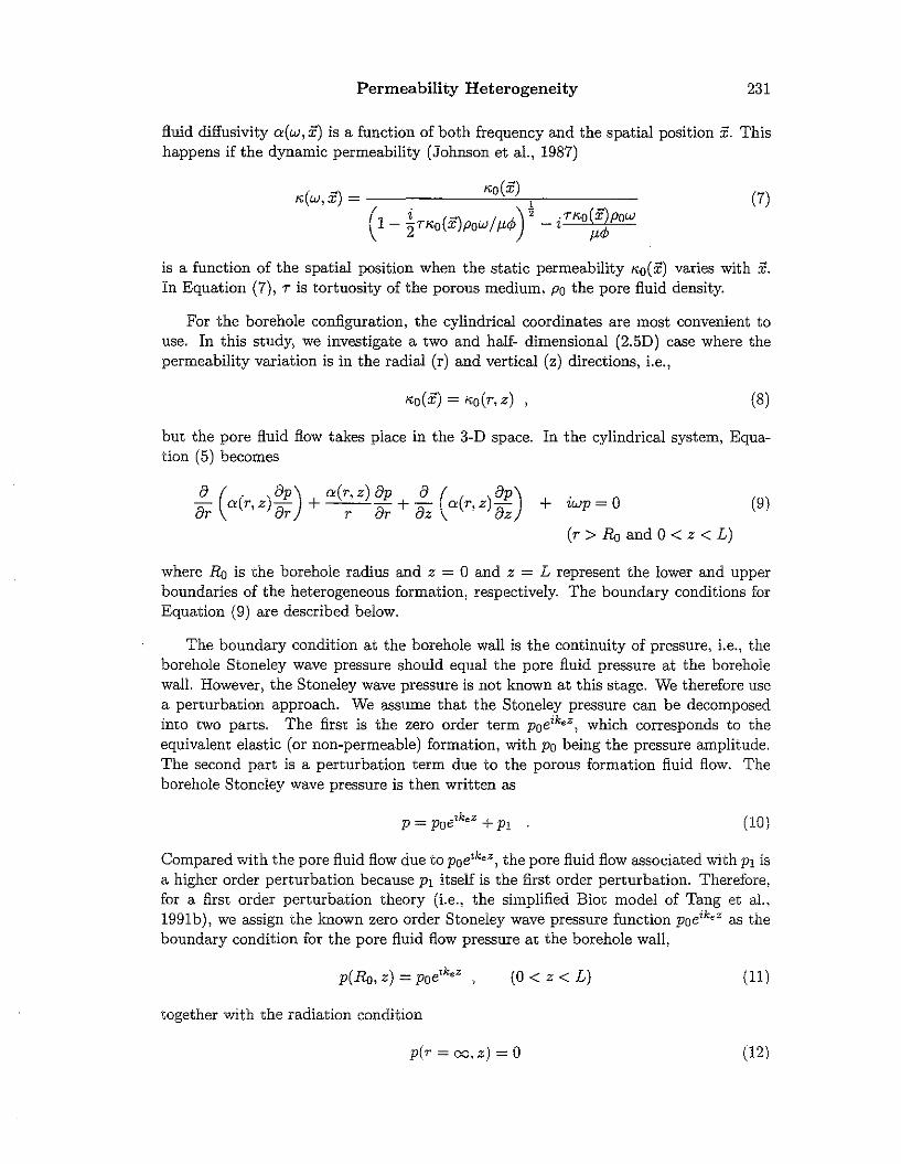
ABSTRACT

An important application of borehole acoustic logging is the determination of formationpermeability using Stoneley waves. Heterogeneous permeable structures, such as frac­tures, sand-shale sequences, etc., are commonly encountered in acoustic logging. Thepurpose of this study is to investigate the effects of the permeability heterogeneities onthe borehole Stoneley wave propagation,

We have studied the effects of formation permeability heterogeneities on the Stone­ley wave propagation when the heterogeneity changes in radial and azimuthal directions(Zhao et aL, 1993). To further study the problem of acoustic logging in heterogeneousporous formations, we study the case where the formation permeability varies in theborehole axial and radial directions. This is a very important problem because verti­cal heterogeneity variations are commonly encountered in acoustic logging applications.Using the finite difference approach, such heterogeneities as random heterogeneous per­meability variations, multiple fracture zones, permeable (sand) - non-permeable (shale)sequences, can be readily modeled, and the results are presented. Our numerical simula­tion results show that the continuous permeability variations in the formation have onlyminimal effects on the Stoneley wave propagation. Whereas the discontinuous variation(e.g., permeable sand and non-permeable shale sequences) can have significant effeces onthe Stoneley wave propagation. However, when the Stoneley wavelength is considerablylarge compared to the scale of heterogeneity variations, the Stoneley wave is sensitiveonly to the overall fluid transmissivity of the formation heterogeneity,

To demonstrate the effects of heterogeneity on the Stoneley wave propagation. anexperimental data set (Winkler et aI., 1989) has been modeled using a randomly layeredpermeability model. The heterogeneous permeability model results agree with the datavery well, while the data disagree with the results from homogeneous permeabilitymodels.

The numerical technique for calculating Stoneley wave propagation across perme­ability heterogeneities has been applied to interpret the acoustic logging data across aheeerogeneous fraceure zone (paillet. 1984). The modeling technique, in conjunctionwith a variable permeability model, successfully explains the non-symmetric patternsof the Stoneley wave attenuation and reileceion at the top and bottom of the fracture

228 Zhao et aI.

zone, while it is difficult to explain these patterns using a homogeneous permeable zonemodel. The technique developed in this study can be used as an effective means forcharacterizing permeability heterogeneities using borehole Stoneley waves.

INTRODUCTION

In a previous study, we investigated the effects of radial and azimuthal variations offormation permeability on the borehole Stoneley wave propagation (Zhao et aI., 1993).In this paper, we will study the situation where the permeability varies in vertical(or borehole axial) and radial directions. This situation is commonly encountered inacoustic logging applications. For example, vertical layering of sedimentary rocks oftenresults in formation sequences that consist of permeable and non-permeable layers (e.g.,sand-shale sequences). Even in formations that are considered homogeneous, perme­ability values measured from well bores often show considerable variations. In manysituations, formation permeability is due to fractures and/or permeable zones that in­tersect the borehole. The characterization of these permeability heterogeneities and thedetermination of their fluid transmissivity are very important tasks in acoustic loggingapplications (Paillet, 1984; Tang and Cheng, 1993), in which the borehole Stoneley waveis commonly used as a primary means for formation permeability studies.

The effects of vertical formation permeability heterogeneity variation on Stoneleywave propagation have been studied by numerous authors. Hornbyet ai. (1989), Tangand Cheng (1988), and Giiler and Toksoz (1987) have studied the propagation of Stone­ley waves across borehole fractures. Tang and Cheng (1993) presented a theory whichcan be used to study the effects of the permeable zone as well as those of fractures.Kostek (1991), by using a finite difference approach, studied the effects of multipleborehole fractures on Stoneley wave propagation. In this work, we will study a moregeneral case in which the formation permeability can have arbitrary variations along thevertical as well as radial directions. As a result, permeability heterogeneities of interest,such as sand-shale sequences, heterogeneous permeable layers, multiple fractures etc.,can be analyzed. The results of these numerical studies will not only demonstrate the ef­fects of the permeability heterogeneities on the borehole Stoneley waves, but also can beused to provide theoretical bases for detecting and characterizing these heterogeneitiesusing Stoneley wave measurements.

As discussed in Zhao et al. (1993), the effects of formation heterogeneity can bestudied using a simplified Biot model approximation (Tang et al., 1991b). By decom­posmg the problem into the elastic and flow problems, we can solve the pore fluid flowproblem for the heterogeneous porous formation independent of the elastic problem.The combination of the solution for the elastic and flow problems will give the solutionfor Stoneley wave propagation with heterogeneous permeability.

The behavior of dynamic fluid flow in heterogeneous porous media has been modeled(Zhao et ai., 1992). Because of the dispersive nature of the flow motion. an iterativefinite difference technique was developed to compute the flow field in the frequencydomam. For the present borehole geometry, we need co solve the dynamic fluid flow

Permeability Heterogeneity 229

problem for the cylindrical coordinate system. The iterative finite difference techniquefor the cylindrical system has been developed (Zhao et al., 1993) to investigate dynamicfluid flow in formations with radial and azimuthal permeability variations. For thepresent study, formation permeability will vary along the borehole axial and radialdirections. Therefore, the iterative finite difference technique used in Zhao et a!., (1993)will be modified for the axial and radial coordinates system. Furthermore, becauseof heterogeneity variation I;l!ong the axial direction and the resulting axial variation ofStoneley wave propagation, we will employ a propagator matrix method to compute theStoneley wave propagation across the permeability heterogeneities.

The effects of the borehole permeability heterogeneity on the Stoneley wave propa­gation can be reflected from the transmission loss (or attenuation) and reflection fromthe heterogeneity boundaries. Both laboratory and field studies have provided suchevidence. In the laboratory, the effects of heterogeneity on Stoneley wave propagationhave been noticed by Winkler et a!., (1989). They evaluated the theory of Stoneleywave propagation in porous boreholes using laboratory experiments and found excel­lent agreement between theory and experiment for 3 out of 4 data sets. However, theyreported that for one data set the data disagree with the results predicted using thehomogeneous model theory. They suggested that sample heterogeneity was the causeof this discrepancy.

In the field study, effects of permeability heterogeneity are commonly encountered inacoustic logging across fractures or fracture zones. Even in isolated fracture zones, thepermeability may have significant variations and these variations can have importanteffects on the Stoneley wave propagation. Such a case was observed by Paillet (1984),who reported an acoustic logging data set across a permeable fracture zone. The data setshows non-symmetric patterns for Stoneley wave attenuation and reflection at the upperand lower boundaries of the fracture zone. Although Tang et a!. (1991a) have used ahomogeneous permeability layer to model the fracture zone and explained the significantStoneley wave attenuation and reflection, the homogeneous layer cannot model theheterogeneity variation within the zone and cannot explain the non-symmetric patterns.

With the numerical analysis developed in this study, we will carry out modelingstudies on the laboratory data set of Winkler et al. (1989) and the field data set ofPaillet (1984). These studies will demonstrate the effects of formation heterogeneity onStoneley wave propagation and the applicability of the numerical technique in handlingformation heterogeneities.

STONELEY WAVE PROPAGATION IN A FORMATION WITHVARIABLE PERMEABILITIES

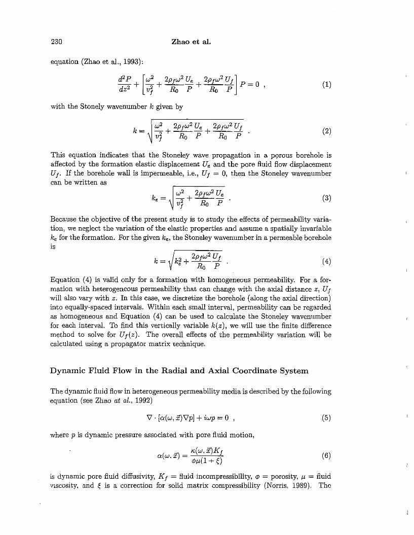
As shown in Zhao et al. (1993), for a Stoneley wave propagating in a permeable porousborehole, the interaction of the Stoneley wave with the formation can be decomposedinto two parts (Tang et al., 1991b). The first is the interaction with an equivalentelastic formation, and the second is the interaction with the dynamic fluid flow into ,heformation. The Stoneley wave can be described by the following one-dimensional wave

230 Zhao et at

equation (Zhao et aI., 1993):

d2p [w

22pfW

2Ue 2pfw

2Uf] _ 0

dz2 + vJ + Ro p + Ro p p - , (1)

with the Stonely wavenumber k given by

k= (2)

This equation indicates that the Stoneley wave propagation in a pc;>rous borehole isaffected by the formation elastic displacement Ue and the pore fluid flow displacementUfo If the borehole wall is impermeable, Le., Uf = 0, then the Stoneley wavenumbercan be written as

(3)

Because the objective of the present study is to study the effects of permeability varia­tion, we neglect the variation of the elastic properties and assume a spatially invariableke for the formation. For the given k., the Stoneley wavenumber in a permeable boreholeis

(4)k= k2 2pfw2 Ufe + Ro p

Equation (4) is valid only for a formation with homogeneous permeability. For a for­mation with heterogeneous permeability that can change with the axial distance z, Ufwill also vary with Z. In this case, we discretize the borehole (along the axial direction)into equally-spaced intervals. Within each small interval, permeability can be regardedas homogeneous and Equation (4) can be used to calculate the Stoneley wavenumberfor each interval. To find this vertically variable k(z), we will use the finite differencemethod to solve for Uf(z). The overall effects of the permeability variation will becalculated using a propagator matrix technique.

Dynamic Fluid Flow in the Radial and Axial Coordinate System

The dynamic fluid flow in heterogeneous permeability media is described by the followingequation (see Zhao at aI., 1992)

\l. [o:(w, x)\lp] + iwp = 0 (5)

where p is dynamic pressure associated with pore fluid motion,

(_) _ K,(w, x)Kf

a w, x - <1>1-'(1 + ~) (6)

is dynamic pore fluid diffusivity, K f = fluid incompressibility, (j) = porosity, I-' = fluidvIscosity, and ~ is a correction for solid matrix compressibility (Norris, 1989). The

Permeability Heterogeneity 231

fluid diffusivity a(w, x) is a function of both frequency and the spatial position X. Thishappens if the dynamic permeability (Johnson et aI., 1987)

(' _) 1£0(x)

K,W,X = 1

~/1 i (-) / ")" .'TKo (x) Pow- -71£0 X POW J1.'I' - ,2 J1.<P

(7)

is a function of the spatial position when the static permeability 1£0(5:) varies with X.In Equation (7), 7 is tortuosity of the porous medium, Po the pore fluid density.

For the borehole configuration, the cylindrical coordinates are most convenient touse. In this study, we investigate a two and half- dimensional (2.5D) case where thepermeability variation is in the radial (r) and vertical (z) directions, i.e.,

I£O(X) = I£o(r, z) , (8)

but the pore fluid flow takes place in the 3-D space. In the cylindrical system, Equa­tion (5) becomes

iJ ( ,i)P) a(r, z) iJp iJ ( iJP)iJr a(r, z) iJr + r iJr + iJz a(r, z) iJz + iwp=O

(r> Ro and 0 < z < L)

(9)

where Ro is the borehole radius and z = 0 and z = L represent the lower and upperboundaries of the heterogeneous formation, respectively. The boundary conditions forEquation (9) are described below.

The boundary condition at the borehole wall is the continuity of pressure, i.e., theborehole Stoneley wave pressure should equal the pore fluid pressure at the boreholewall. However, the Stoneley wave pressure is not known at this stage. We therefore usea perturbation approach. We assume that the Stoneley pressure can be decomposedimo two parts. The first is the zero order term poeik,z, which corresponds to theequivalem elastic (or non-permeable) formation, with Po being the pressure amplitude.The second part is a perturbation term due to the porous formation fluid flow. Theborehole Stoneley wave pressure is then written as

p = poe~kez + Pl (10)

Compared with the pore fluid flow due to poe'k,z, the pore fluid flow associated with PI isa higher order perturbation because PI itself is the first order perturbation. Therefore,for a first order perturbation theory (i.e., the simplified Biot model of Tang et aI.,1991b), we assign the known zero order Stoneley wave pressure function poeik,z as theboundary condition for the pore fluid flow pressure at the borehole wall,

p(Ro, z) = poe'k,z

together with the radiation condition

(O<z<L) (11)

p(r = oo.z) = 0 (12)

232

and the no-flow boundary conditions

Zhao et aI.

--,oP,-,(,-,r,::-z_=_O--,-) _ op(r, z = L) _ °oz - oz - (13)

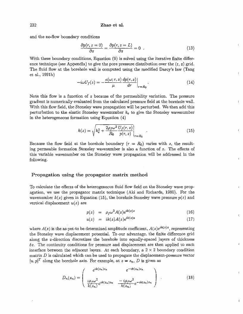
With these boundary conditions, Equation (9) is solved using the iterative finite differ­ence technique (see Appendix) to give the pore pressure distribution over the (r, z) grid.The fluid flow at the borehole wall is computed using the modified Darcy's law (Tanget aI., 1991b)

. U ( ) x;(w;r,z) dp(r,z) I-'w f z = - d .M r r=Ro

(14)

(15)

Note this flow is a function of z because of the permeability variation. The pressuregradient is numerically evaluated from the calculated pressure field at the borehole wall.With this flow field, the Stoneley wave propagation will be perturbed. We then add thisperturbation to the elastic Stoneley wavenumber ke to give the Stoneley wavenumberin the heterogeneous formation using Equation (4)

k( ) - Vfk2 2pfw2Uf(r, z) Iz-\ e+-O::- ( )1

"'0 P r, z ir=Ro

Because the flow field at the borehole boundary (r = Ro) varies with z, the result­ing permeable formation Stoneley wavenumber is also a function of z. The effects ofthis variable wavenumber on the Stoneley wave propagation will be addressed in thefollowing.

Propagation using the propagator matrix method

To calculate the effects of the heterogeneous fluid flow field on the Stoneley wave prop­agation, we use the propagator matrix technique (Aki and Richards, 1980). For thewavenumber k(z) given in Equation (15), the borehole Stoneley wave pressure p(z) andvertical displacement u(z) are

p(z) = Pfw2A(z)eik(Z)Z

u(z)ik(z)A(z)eik(z)z

(16)

(17)

where A(z) is the as-yet-to be determined amplitude coefficient, A(z)eik(Z)Z; representing,he Stoneley wave displacement potential. To our advantage, the finite difference gridalong the z-direction discretizes the borehole into equally-spaced layers of thicknessoz. The continuity conditions for pressure and displacement are then applied to eachinterface between the adjacent layers. At each boundary, a 2 x 2 boundary conditionmatrix D is calculated which can be used to propagate the displacement-pressure vector[u, p]T along the borehole axis. For example, at z = Zn, D is given as

( eik(z".)Zn e-tk(Zn)Zn

JDn(zn) = (18)

~ 1PfW ; e,k(znlZn io w2~ , f , e-tk(Zn}Zn

k(zn k(Zni ,

Permeability Heterogeneity 233

(20)

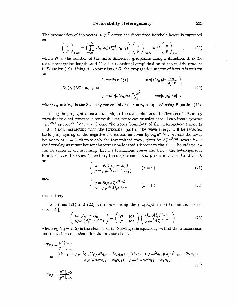
The propagation of the vector [u, pjT across the discretized borehole layers is expressedas

( u ) = (fi Dn(Zn)D;;-l(zn_l)) ( u ) = G ( u) _' (19)P z=o n=l p z=L p z=1-

where N is the number of the finite difference gridpoints along z-direction, L is thetotal propagation length, and G is the notational simplification of the matrix productin Equation (19). Using the expression of D, the propagation matrix oflayer n is writtenas

rcos[k(zn)8z] sin[k(zn)8z]~ J

PfwDn(zn)D;;-l(zn_l) =

PfW2

\ -sin[k(zn)8z] kn

cos[k(zn)8z]

where kn = k(zn) is the Stoneley wavenumber at z = Zn computed using Equation (15).

Using the propagator matrix technique, the transmission and reflection of a Stoneleywave due to a heterogeneous permeable structure can be calculated. Let a Stoneley waveAte,k,z approach from z < 0 onto the upper boundary of the heterogeneous zone (z= 0). Upon interacting with the structure, part of the wave energy will be reflectedback, propagating in the negative z direction as given by Ail e-ik,z. Across the iowerboundary at z = L, there is only the transmitted wave, given by Aj;,eikNz , where kN isthe Stoneley wavenumber for the formation located adjacent to the z = L boundary. kNcan be oaken as ke , assuming that the formations above and below the heterogeneousformation are the same. Therefore, the displacemem and pressure at z = a and z = Lare

and

respectively,

(z = 0)

(z = L)

(21)

(22)

EquatlOns (21) and (22) are related using the propagator matrix method [Equa­,ion (19)],

(' 'ke(A(j - Ail) )\ = (gll g12) (ikNAj;,e'kNL ') (23), Pfw

2(At + Ail) \ g21 g22 ) " Pfw2Aj;,e'kNL

where giJ (i,j = 1, 2) is the element of G. Solving this equation, we find the transmissionand reflection coefficiems for the pressure field,

iT' pT :z=L.L rs = '-,-""-=.

p+lz=o(ikegn + Pfw2g12) (pfw2g22 - ikeg21 ) - (ikeg21 + pfw2g22)(ptW2g12 - ikegn )

=ikN lpfw2g22 - ikeg21 ) - Pfw2(Pfw2g12 - ikegn )

(241

'-, :..P.,.-.;.:!z_=c:.oH.ej = +i.p Iz=O

234

=

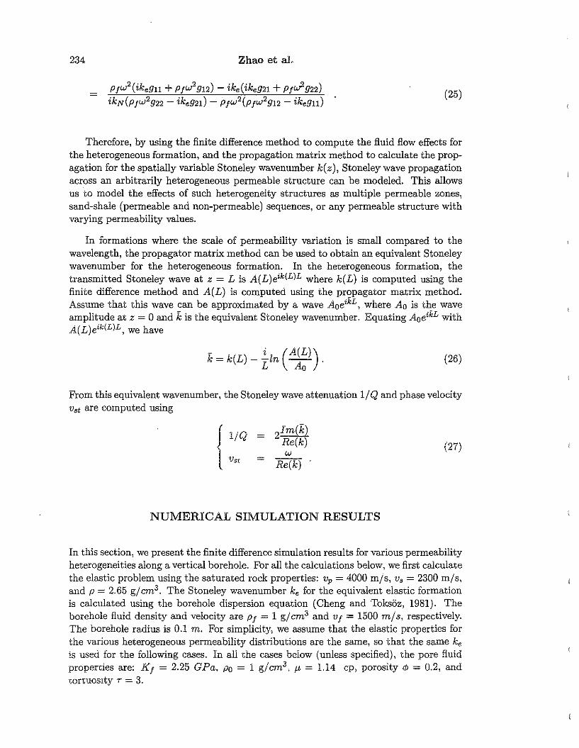
Zhao et al.

Pfw2(ike911 + Pfw2912) - ike(ike921 + Pfw2922)

ikN(Pfw2g22 - ike921) - Pfw2(Pfw2g12 - ike911)(25)

Therefore, by using the finite difference method to compute the fluid flow effects forthe heterogeneous formation, and the propagation matrix method to calculate the prop­agation for the spatially variable Stoneley wavenumber k(z), Stoneley wave propagationacross an arbitrarily heterogeneous permeable structure can be modeled. This allowsus 'to model the effects of such heterogeneity structures as multiple permeable zones,sand-shale (permeable and non-permeable) sequences, or any permeable structure withvarying permeability values.

In formations where the scale of permeability variation is small compared to thewavelength, the propagator matrix method can be used to obtaln an equivalent Stoneleywavenumber for the heterogeneous formation. In the heterogeneous formation, thetransmitted Stoneley wave at z = L is A(L)eik(LlL where k(L) is computed using thefinite difference method and A(L) is computed using the propagator matrix method.Assume that this wave can be approximated by a wave AoeikL , where Ao is the waveamplitude at z = 0 and k is the equivalent Stoneley wavenumber. Equating AoeikL withA(L)eik(LlL, we have

(26)

From this equivalent wavenumber, the Stoneley wave attenuation 1/Q and phase velocityVst are computed using

2Im(k)Re(k)w

- Re(k)

(27)

NUMERICAL SIMULATION RESULTS

In this section, we present the finite difference simulation results for various permeabilityheterogeneities along a vertical borehole. For all the calculations below, we first calculatethe elastic problem using the saturated rock properties: vp = 4000 mis, V s = 2300 mis,and P = 2.65 g/cm3. The Stoneley wavenumber ke for the equivalent elastic formationis calculated using the borehole dispersion equation (Cheng and Toksoz, 1981). Theborehole fluid density and velocity are Pf = 1 g/cm3 and vf = 1500 mis, respectively.The borehole radius is 0.1 m. For simplicity, we assume that the elastic properties forthe various heterogeneous permeability distributions are the same, so that the same ke

is used for the following cases. In all the cases below (unless specified), the pore fluidproperties are: Kf = 2.25 GPa. Po = 1 g/cm3, J.L = 1.14 cp, porosity r/J = 0.2, andtortUosIty T = 3.

Permeability Heterogeneity

Homogeneous Permeability - A Test of the Numerical Algorithm

235

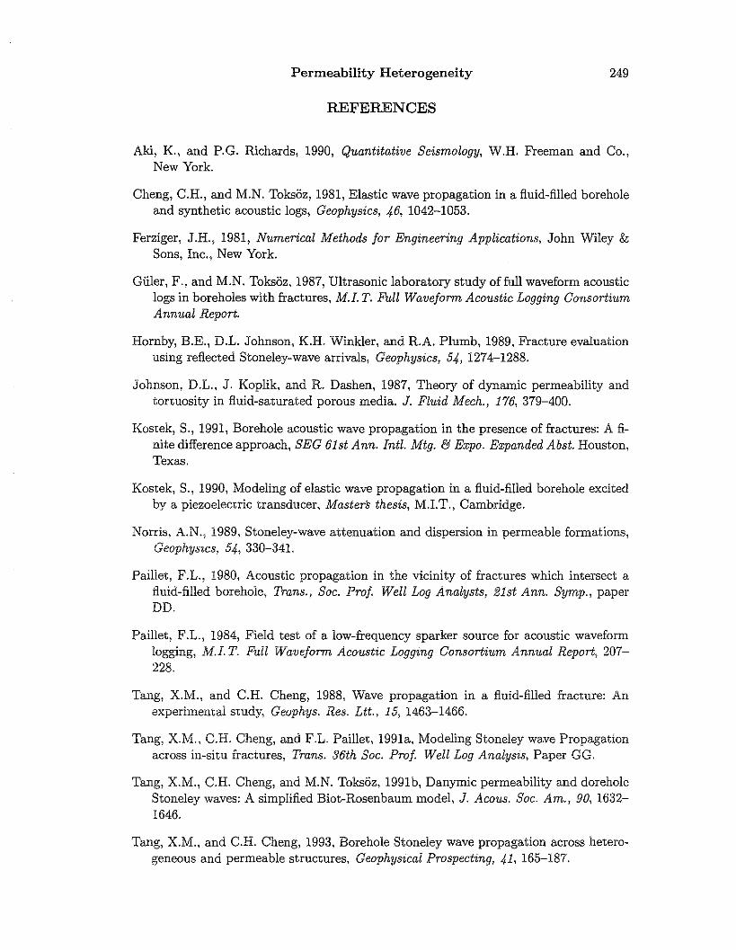
We first present the simulation result for a homogeneous permeable formation surround­ing the borehole. This example, together with the existing analytical solution, offers atest of the validity and accuracy of the finite difference simulation algorithm.

Figure 1 shows the comparison between the Stoneley wave phase velocity (a) andattenuation (b) calculated using the analytical solution (see Zhao et aI., 1993) and thoseusing the finite difference method, and equivalent wavenumber formula (Equation 26)for a homogeneous permeability model. These results are calculated for the frequencyrange of 0 ~ 5 kHz in which most Stoneley wave measurements are performed. Theformation permeability is 1 Darcy. For simplicity, the effects due to solid matrix com­pressibility are neglected (I.e., ,; = 0 in Equation 6) when calculating both the analyticaland finite difference results. The results for the two different approaches are in excel­lent agreement. This comparison demonstrates the validity and accuracy of the finitedifference technique. Therefore, in the case of a heterogeneous permeability distribu­tion where an analytical solution is difficult to find, we will rely on the finite differencemethod to calculate the Stoneley wave propagation.

Variable Permeability Models

In the field acoustic logging applications, the formation permeability is usually heteroge­neous. For example, the permeability may fluctuate from place to place due to randomvariations. The permeability may have cyclic variations due to sand-shale sequences.The effects of these heterogeneity variations on the borehole Stoneley wave propagationare studied here. In this section, we assume that the logging tool is within the het­erogeneous formation and we will analyze the average Stoneley wave attenuation andvelocity dispersion characteristics using Equations (26) and (27).

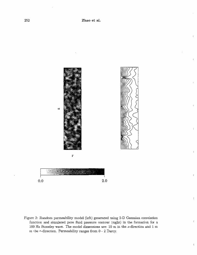
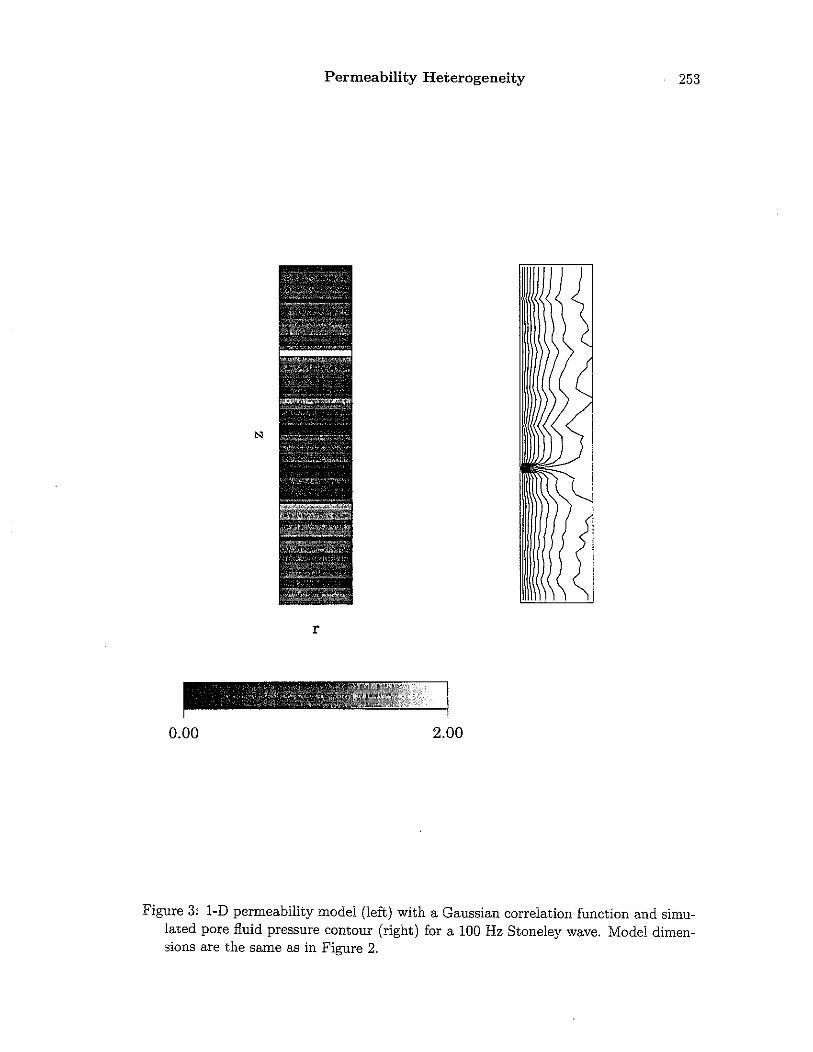
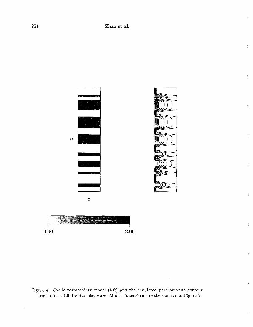
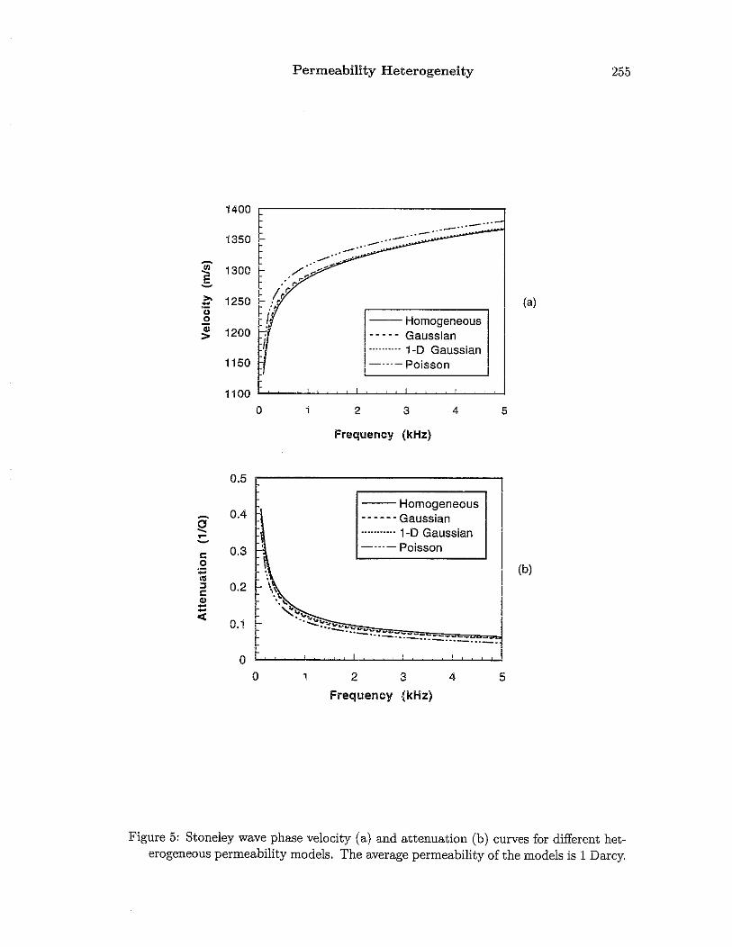
In Figures 2, 3, and 4, three formation permeability heterogeneity models are shown.They are the 2-D random variation with a Gaussian correlation function of correlationlength of 0.2 m (Figure 2), the 1-D random variation along borehole axial direction withGaussian correlation function of correlation length 0.1 m (Figure 3), and the permeableand non-permeable layer model generated using the Poisson process. All three modelshave the same average permeability of 1 Darcy. For the continuous models, the standarddeviation of the variation is 30%. For the discontinuous model, the permeability contrastbetween high and low permeability layers is 100:1. For the borehole Stoneley wave, theaxial propagation distance is much greater than the depth of fluid motion penetrationin the radial direction. We therefore set the axial and radial model dimensions as10 m and 1 m, respectively. In Figures 2, 3, and 4, the models are shown only fora 5 m section in the axial direction. In these figures, the calculated dynamic fiuidpressure amplitude distribution for those heterogeneous models is also plotted. Thefrequency for the fl uid motion is 1 kHz. As can be seen from these figures, the formationfluid pressure distributions are distinctly different from one another because of thedifferent heterogeneity variations. The 2-D random model shows considerable fluidpressure variation in both radial and axial directions. The I-D model shows less axial

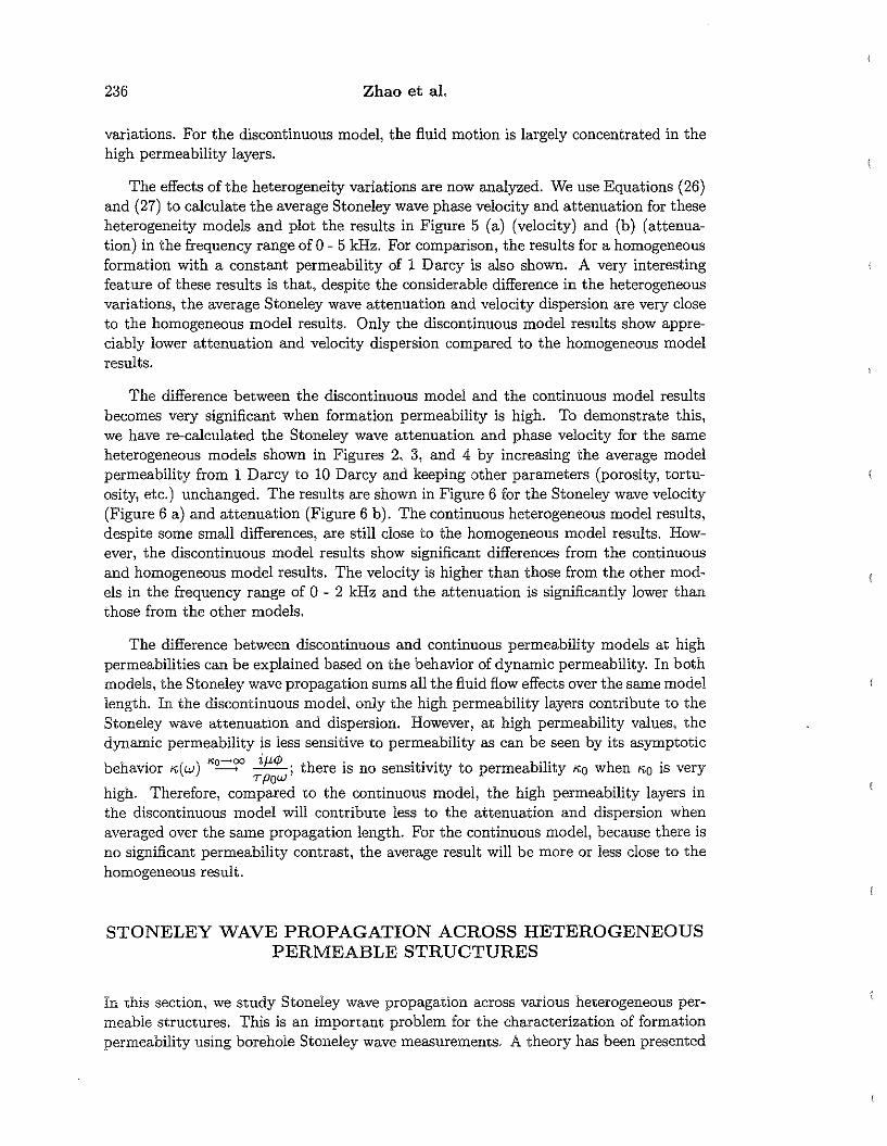
236 Zhao et al.

variations. For the discontinuous model, the fluid motion is largely concentrated in thehigh permeability layers.

The effects of the heterogeneity variations are now analyzed. We use Equations (26)and (27) to calculate the average Stoneley wave phase velocity and attenuation for theseheterogeneity models and plot the results in Figure 5 (a) (velocity) and (b) (attenua­tion) in the frequency range of 0 - 5 kHz. For comparison, the results for a homogeneousformation with a constant permeability of 1 Darcy is also shown. A very interestingfeature of these results is that, despite the considerable difference in the heterogeneousvariations, the average Stoneley wave attenuation and velocity dispersion are very closeto the homogeneous model results. Only the discontinuous model results show appre­ciably lower attenuation and velocity dispersion compared to the homogeneous modelresults.

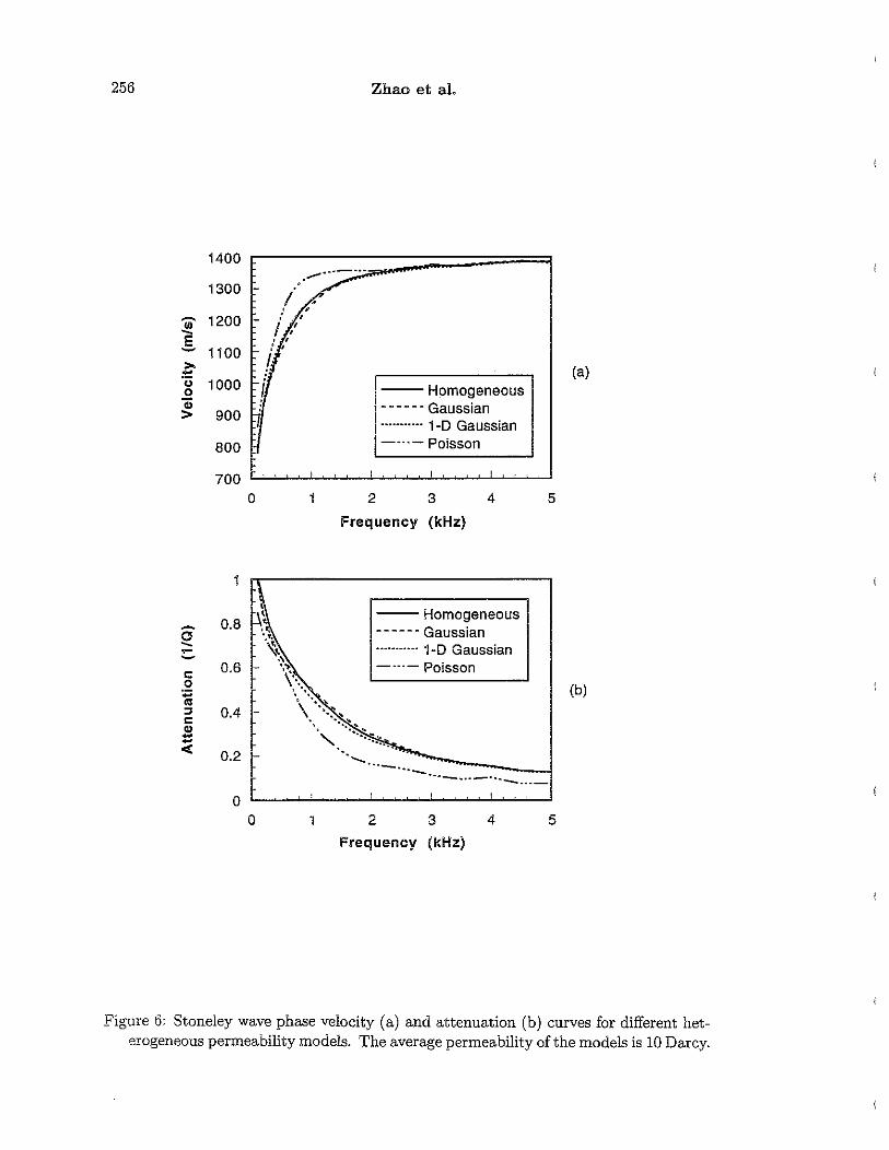
The difference between the discontinuous model and the continuous model resultsbecomes very significant when formation permeability is high. To demonstrate this,we have re-calculated the Stoneley wave attenuation and phase velocity for the sameheterogeneous models shown in Figures 2, 3, and 4 by increasing the average modelpermeability from 1 Darcy to 10 Darcy and keeping other parameters (porosity, tortu­osity, etc.) unchanged. The results are shown in Figure 6 for the Stoneley wave velocity(Figure 6 a) and attenuation (Figure 6 b). The continuous heterogeneous model results,despite some small differences, are still close to the homogeneous model results. How­ever, the discontinuous model results show significant differences from the continuousand homogeneous model results. The velocity is higher than those from the other mod­els in the frequency range of 0 - 2 kHz and the attenuation is significantly lower thanthose from the other models.

The difference between discontinuous and continuous permeability models at highpermeabilities can be explained based on the behavior of dynamic permeability. In bothmodels, the Stoneley wave propagation sums all the fluid flow effects over the same modellength. In the discontinuous model, only the high permeability layers contribute to theStoneley wave attenuatIOn and dispersion. However, at high permeability values, thedynamic permeability is less sensitive to permeability as can be seen by its asymptotic

behavior ;,;(w) ~'C..,oo il-'<P; there is no sensitivity to permeability ;';0 when "0 is veryTPOW

high. Therefore, compared to the continuous model, the high permeability layers inthe discontinuous model will contribute less to the attenuation and dispersion whenaveraged over the same propagation length. For the continuous model, because there isno significant permeability contrast, the average result will be more or less close to thehomogeneous result.

STONELEY WAVE PROPAGATION ACROSS HETEROGENEOUSPERMEABLE STRUCTURES

In thIS section, we study Stoneley wave propagation across various heterogeneous per­meable structures. This is an important problem for the characterization of formationpermeability using borehole Stoneley wave measurements. A theory has been presented

Permeability Heterogeneity 237

by Tang and Cheng (1993) to model borehole fractures as a highly permeable zone.This theory is able to explain the observed Stoneley wave transmission and reflection atfractures. A drawback of this model is that it uses a homogeneous permeability layerto model the permeable zone and therefore neglects the permeability variation withinthe zone. In reality, a natural permeable structure may contain various heterogeneousstructures. With the heterogeneous propagation theory developed in this study, we canstudy the effects of the heterogeneity structures and compare the similarity and differ­ence between the simple homogeneous model and the heterogeneity structure model.

Comparison with the Homogeneous Permeable Zone Model

According to Tang and Cheng (1993), the Stoneley wave transmission and reflectioncoefficients due to a homogeneous permeable layer are given by

4klk2e-ik2LTrs = (28)

(kl + k1)2e ik2L - (k1 - k2?eik2L

2i(k5 - kr)sin(k2L)Ref = (29)

(k1 + k2)2e ik2L - (kl - k2)2eik2L

where k1 is the Stoneley wavenumber outside the permeable zone, k2 is the permeablezone Stoneley wavenumber, and L is the zone thickness. In fact, the simple homoge­neous permeable model results can be derived as the special case for the propagatormatrix results (Equations 24 and 25). Therefore, the analytical results presented inEquations (28) and (29) can be used to test the validity and accuracy of the finitedifference and propagator matrix approach developed in this study.

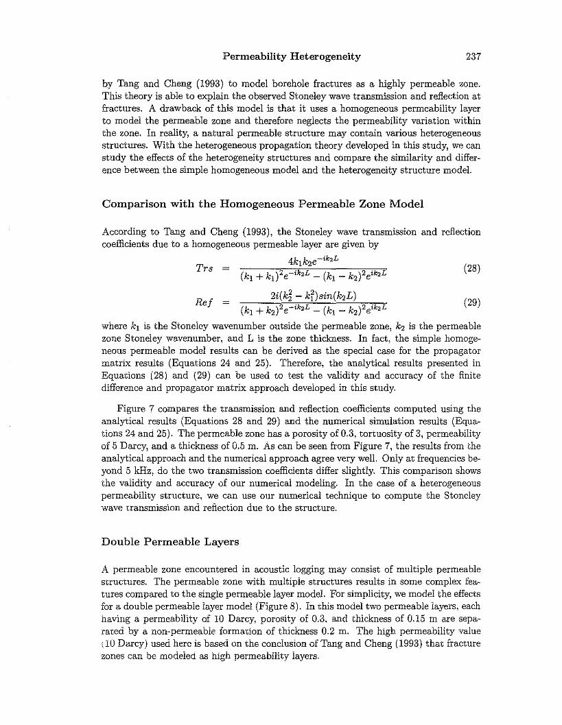
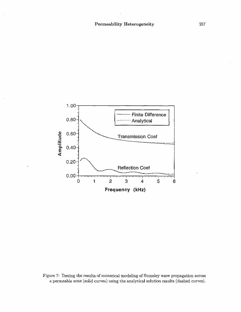
Figure 7 compares the transmission and reflection coefficients computed using theanalytical results (Equations 28 and 29) and the numerical simulation results (Equa­tions 24 and 25). The permeable zone has a porosity of 0.3, tonuosity of 3, permeabilityof 5 Darcy, and a thickness of 0.5 m. As can be seen from Figure 7, the results from theanalytical approach and the numerical approach agree very well. Only at frequencies be­yond 5 kHz, do the two transmission coefficients differ slightly. This comparison showsthe validity and accuracy of our numerical modeling. In the case of a heterogeneouspermeability structure, we can use our numerical technique to compute the Stoneleywave transmission and reflection due to the structure.

Double Permeable Layers

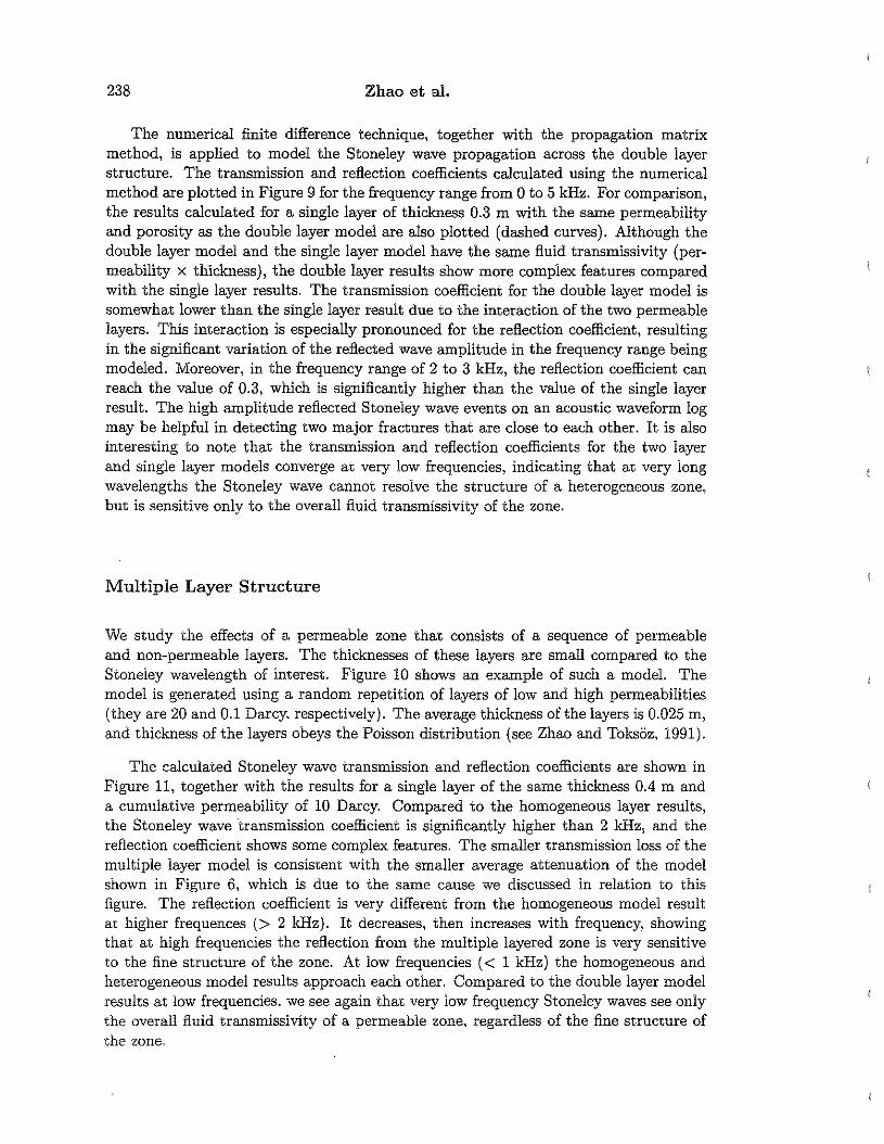
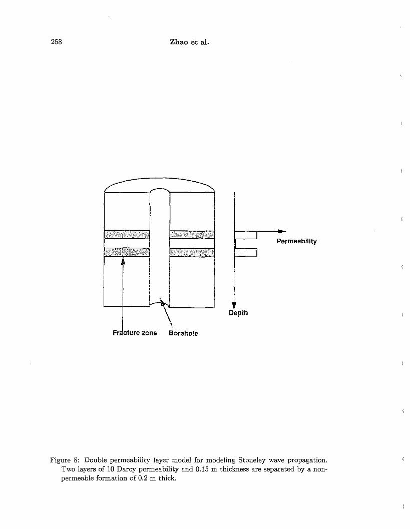
A permeable zone encountered in acoustic logging may consist of multiple permeablestructures. The permeable zone with multiple structures results in some complex fea­tures compared to the single permeable layer model. For simplicity, we model the effectsfor a double permeable layer model (Figure 8). In this model two permeable layers, eachhaving a permeability of 10 Darcy, porosity of 0.3. and thickness of 0.15 m are sepa­rated by a non-permeable formation of thickness 0.2 m. The high permeability value\10 Darcyj used here is based on the conclusion of Tang and Cheng (1993j that fracturezones can be modeled as high permeability layers.

238 Zhao et al.

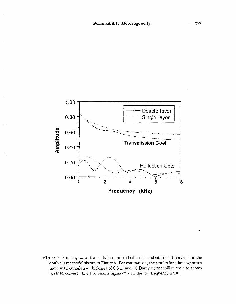
The numerical finite difference technique, together with the propagation matrixmethod, is applied to model the Stoneley wave propagation across the double layerstructure. The transmission and reflection coefficients calculated using the numericalmethod are plotted in Figure 9 for the frequency range from 0 to 5 kHz. For comparison,the results calculated for a single layer of thickness 0.3 m with the same permeabilityand porosity as the double layer model are also plotted (dashed curves). Although thedouble layer model and the single layer model have the same fluid transmissivity (per­meability X thickness), the double layer results show more complex features comparedwith the single layer results. The transmission coefficient for the double layer model issomewhat lower than the single layer result due to the interaction of the two permeablelayers. This interaction is especially pronounced for the reflection coefficient, resultingin the significant variation of the reflected wave amplitude in the frequency range beingmodeled. Moreover, in the frequency range of 2 to 3 kHz, the reflection coefficient canreach the value of 0.3, which is significantly higher than the value of the single layerresult. The high amplitude reflected Stoneley wave events on an acoustic waveform logmay be helpful in detecting two major fractures that are close to each other. It is alsointeresting to note that the transmission and reflection coefficients for the two layerand single layer models converge at very low frequencies, indicating that at very longwavelengths the Stoneley wave cannot resolve the structure of a heterogeneous zone,but is sensitive only to the overall fluid transmissivity of the zone.

Multiple Layer Structure

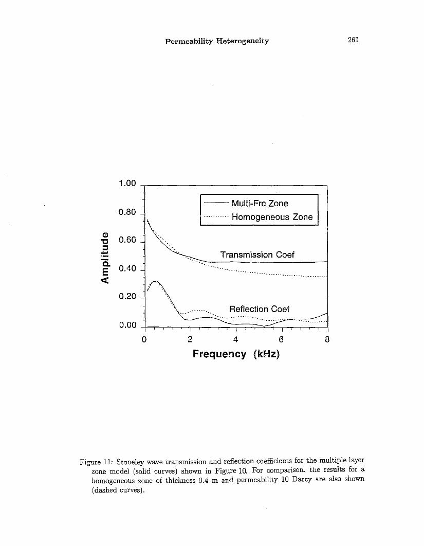
We study the effects of a permeable zone that consists of a sequence of permeableand non-permeable layers. The thicknesses of these layers are small compared to theStoneley wavelength of interest. Figure 10 shows an example of such a model. Themodel is generated using a random repetition of layers of low and high permeabilities(they are 20 and 0.1 Darcy, respectively). The average thickness of the layers is 0.025 m,and thickness of the layers obeys the Poisson distribution (see Zhao and Toksoz. 1991).

The calculated Stoneley wave transmission and reflection coefficients are shown inFigure 11, together with the results for a single layer of the same thickness 0.4 m anda cumulative permeability of 10 Darcy. Compared to the homogeneous layer results,the Stoneley wave transmission coefficient is significantly higher than 2 kHz, and thereflection coefficient shows some complex features. The smaller transmission loss of themultiple layer model is consistent with the smaller average attenuation of the modelshown in Figure 6, which is due to the same cause we discussed in relation to thisfigure. The reflection coefficient is very different from the homogeneous model resultat higher frequences (> 2 kHz). It decreases, then increases with frequency, showingthat at high frequencies the reflection from the multiple layered zone is very sensitiveto the fine structure of the zone. At low frequencies « 1 kHz) the homogeneous andheterogeneous model results approach each other. Compared to the double layer modelresults at low frequencies. we see again that very low frequency Stoneley waves see onlythe overall fluid transmissivity of a permeable zone. regardless of the fine structure ofthe zone,

Permeability Heterogeneity

Random Permeability Structure

239

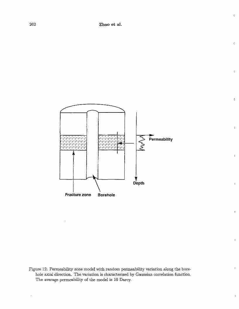
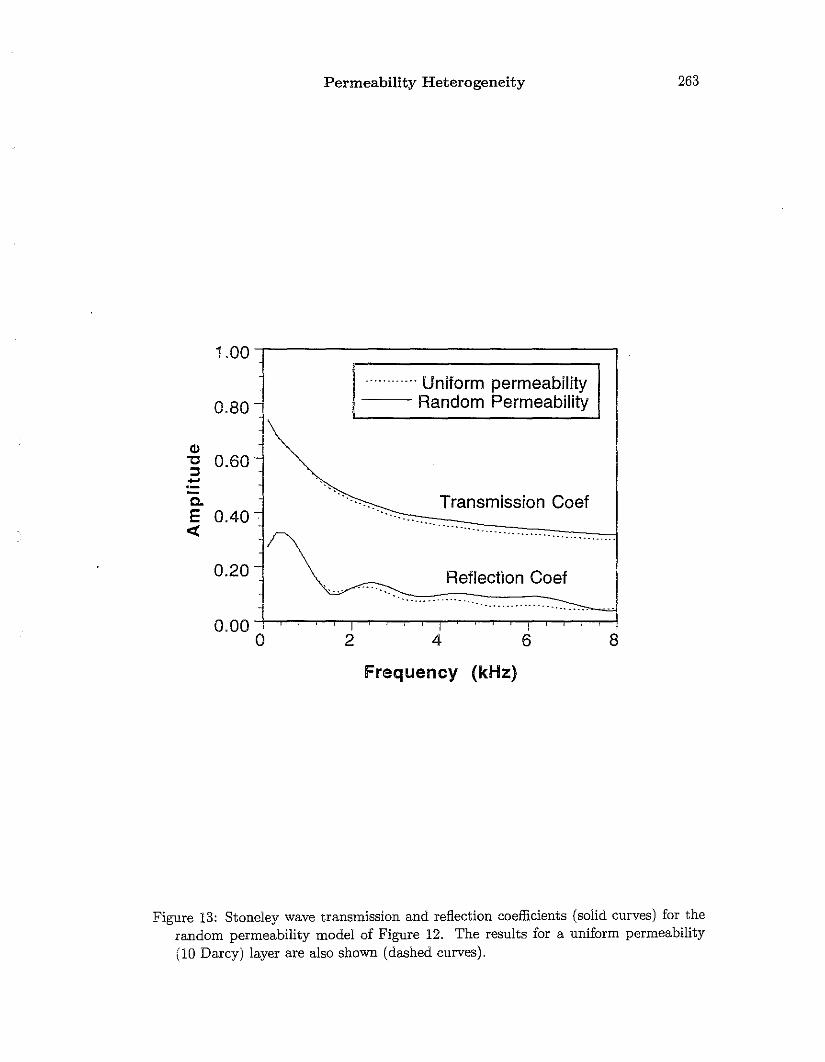
We now study the case where the permeability within the permeable zone can haverandom but continuous variations. We model this situation using the I-D continuousrandom model generated using the I-D Gaussian correlation function (see Zhao andToksoz, 1991). The permeability variation is shown in Figure 12 which has an averagevalue of 10 Darcy and a standard deviation of 28%. This permeability variation isassigned to a permeable zone 0.4 m thick with a porosity value of 0.3. Figure 13shows the resulting Stoneley wave transmission and reflection coefficients across theheterogeneous zone. For comparison, we also plot the results (dashed curves) calculatedusing a homogeneous layer model (Equations 28 and 29), in which we used the averagepermeability of 10 Darcy and the same thickness of 0.4 m for the layer.

Despite the considerable permeability variation within the permeable zone, the het­erogeneous model results are not very different from the homogeneous model results,except the transmission and reflection coefficients for the heterogeneous model are alittle higher than the homogeneous model result beyond 2 kHz. At low frequencies, es­pecially approaching the zero frequency, the results from both models converge towardeach other. This convergence occurs at higher frequency than the previous' double layerand multiple layer models.

Model Comparison

To further investigate the similarity and difference of Stoneley wave propagation acrossthe different heterogeneity models, we plot the Stoneley wave amplitude change ver­sus dist.ance across the permeable zone in Figure 14 for these models. The amplitudevs. distance curves are calculated for a 5 kHz Stoneley wave using the propagator ma­trix method t.o compute the transmit.ted wave amplitude Equation (24) at each finitedifference grid inside the permeable zone.

We compare three situat.ions: (1) the mult.iple layer structure given in Figure 10; (2)the random permeabilit.y variation model given in Figure 12; and (3) the homogeneouslayer model. The paramet.ers for all three models are the same (I.e., same porosity,thickness. and average permeability, etc). As shown in Figure 14, when the Stoneleywave enters t.he permeable zone, the amplitude begins to decrease. For the randompermeability model. although the het.erogeneous variation is evident on the amplitude,the overall result (dashed line) is not very different from the homogeneous model result,because of t.he cont.inuous permeability variation. For the multiple layer model, whichhas a discont.inuous permeability variation, the amplitude VS. dist.ance curve is distinctlydifferent from the homogeneous and the continuous model result.s. The amplitude isattenuat.ed in the permeable layer, but remains constant. in the non-permeable layers,resulting in a st.ep-like decrease of t.he wave amplit.ude. As a result, t.he total amplitudereduction is less than those of the ot.her two models. This result is also consistent. withthe Stoneley wave attenuation results plotted in Figure 6 which show that for the sameaverage permeability the discont.inuous permeability model has lower attenuation thanthose from t.he continuous models.

240 Zhao et al.

In the following application section, we will use the discontinuous permeability modelto study the laboratory and field 8toneley wave data, which could not be explalned usingthe homogeneous model theory. We will show that only the discontinuous permeabilitymodel theory can explaln the data very well.

APPLICATION TO ACOUSTIC LOGGING DATA FROMHETEROGENEOUS FORMATIONS

Data from Laboratory Experiments

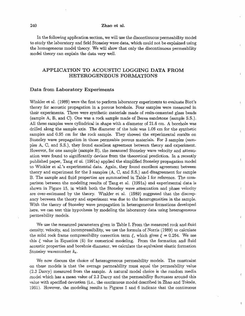
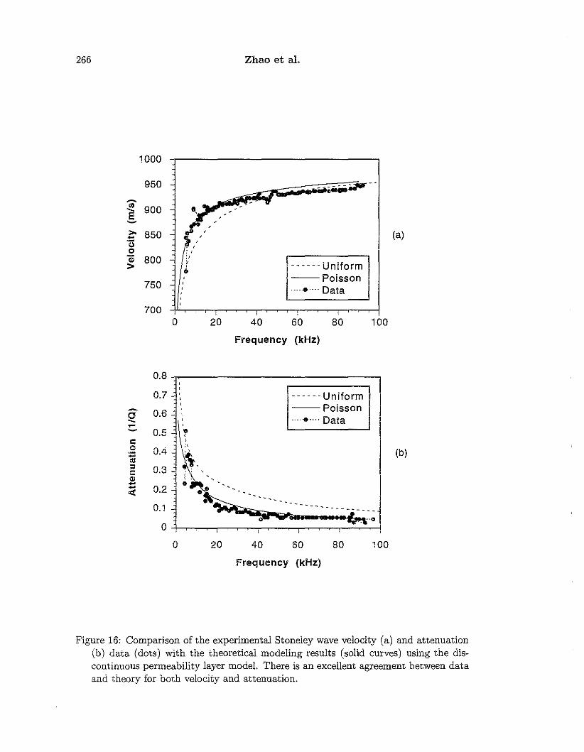
Winkler et al. (1989) were the first to perform laboratory experiments to evaluate Biot'stheory for acoustic propagation in a porous borehole. Four samples were measured intheir experiments. Three were synthetic materials made of resin-cemented glass beads(sample A, B, and C). One was a rock sample made of Berea sandstone (sample 8.8.).All these samples were cylindrical in shape with a diameter of 21.6 cm. A borehole wasdrilled along the sample axis. The diameter of the hole was 1.06 cm for the syntheticsamples and 0.95 cm for the rock sample. They showed the experimental results on8toneley wave propagation in those permeable porous materials. For 3 samples (sam­ples A, C, and 8.8.), they found excellent agreement between theory and experiment.However, for one sample (sample B), the measured 8toneley wave velocity and attenu­ation were found to significantly deviate from the theoretical prediction. In a recentlypublished paper, Tang et ai. (1991a) applied the simplified 8toneley propagation modelto Winkler et al. 's experimental data. Again, they found excellent agreement betweentheory and experiment for the 3 samples (A, C, and 8.8.) and disagreement for sampleB. The sample and fluid properties are summarized in Table I for reference. The com­parison between the modeling results of Tang et al. (1991a) and experimental data isshown in Figure 15, in which both the 8toneley wave attenuation and phase velocityare over-estimated by the theory. Winkler et ai. (1989) suggested that the discrep­ancy between the theory and experiment was due to the heterogeneities in the sample.With the theory of 8toneley wave propagation in heterogeneous formations developedhere, we can test this hypothesis by modeling the laboratory data using heterogeneouspermeability models.

We use the measured parameters given in Table 1. From the measured rock and fluiddensity, velocity, and incompressibility, we use the formula of Norris (1989) to calculatethe solid rock frame compressibility correction term ~, which gives ~ = 0.264. We usethis ~ value in Equation (6) for numerical modeling. From the formation and fluidacoustic properties and borehole diameter, we calculate the equivalent elastic formation8toneley wavenumber ke .

We now discuss the choice of heterogeneous permeability models. The constrainton these models is that the average permeability must equal the permeability value(2.3 Darcy) measured from the sample. A natural model choice is the random mediamodel which has a mean value of 2.3 Darcy and the permeability fluctuates around thisvalue with specified deviation (i.e.. the continuous model described in Zhao and Toksiiz,1991). However, the modeling results in Figures 5 and 6 indicate that the continuous

Permeability Heterogeneity 241

permeability model results do not differ greatly from the homogeneous model results.Based on the modeling results, we exclude these models from the candidacy. On theother hand, the discontinuous permeability model results in these figures (especiallyFigure 6) show significantly less attenuation and dispersion compared with the homo­geneous model results, as is also the case for the data shown in Figure 15. We thereforechoose the 1-D discontinuous model to model the experimental data.

In our modeling, the numerical model length L is taken as 0.2 m, which is approxi­mately the array aperture spanned by the scanning receiver in the experiment (Winkleret aI., 1989). The radial model size is about 10 times that of the borehole diameter.The heterogeneous permeability model is generated using the Poisson process with anaverage thickness of 0.01 m. The high permeability layers have a permeability value of .4.6 Darcy, while the low permeability layers, 0.01 Darcy; the average is about 2.3 Darcy.

The modeled Stoneley wave velocity and attenuation are shown together with themeasured data in Figure 16. There is excellent agreement between theory and data. Itis worthwhile to note that this agreement holds for both phase velocity and attenuation.It is also worthwhile to point out that the same excellent agreement was obtained whendifferent I-D Poisson models with different average layer thicknesses are used in thenumerical modeling. In these models, 50% of the formation has high permeability andthe other 50%, low permeability.

Our numerical modeling results support the hypothesis of Winkler et al. (1989)that the sample heterogeneity was the cause of discrepancy between experimental dataand theory for a homogeneous formation. In addition, our modeling also suggests thatthe effects of the heterogeneities are such that some portions of the borehole are verypermeable and other portions are impermeable, similar to the Poisson layering modelsused in the numerical modeling.

Data from the VRL-MIl Well

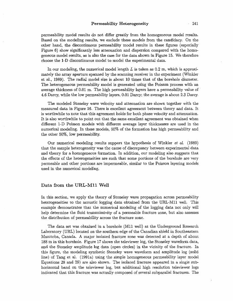
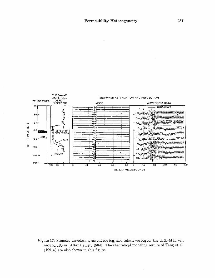
In this section, we apply the theory of Stoneley wave propagation across permeabilityheterogeneities to the acoustic logging data obtained from the URL-Mll well. Thisexample demonstrates that the numerical modeling of the logging data not only willhelp determine the fluid transmissivity of a permeable fracture zone, but aiso assessesthe distribution of permeability across the fracture zone.

The data set was obtained in a borehole (Mll well) at the Underground ResearchLaboratory (URL) located on the southern edge of the Canadian shield in SoutheasternManitoba, Canada. A major isolated fracture zone was detected at a depth of about188 m in this borehole. Figure 17 shows the televiewer log, the Stoneley waveform data,and the Stoneley amplitude log data (open circles) in the vicinity of the fracture. Inthis figure, the modeling synthetic Stoneley wave waveform and amplitude log (solidline) of Tang et al. (1991a) using the simple homogeneous permeability layer modelEquations 28 and 29) are also shown. The isolated fracture appeared in a single sub­horizontal band on the televiewer log, but additional high resolution televiewer logsindicated that this fracture was actually composed of several subparallel fractures. The

242 Zhao et al.

logging waveforms were obtained using a sparker source at 5 kHz; the borehole andthe tool diameters were 15.2 and 5.1 cm, respectively. The source-receiver spacing was2.14 m.

As Seen from the logging waveforms, the Stoneley waveS are significantly attenuatedacross the fractures. A Stoneley wave reflection at the top can also be observed, asindicated by the line drawn on the waveform logs in Figure 17, which marks the moveoutof the reflected waves. A feature that is of special interest in this study is that the fielddata do not have a clearly traceable down-going reflection, whereas the homogeneouslayer theory of Tang et aI. (1991a) predicts a symmetric pattern for the up-going anddown-going reflections (Figure 17, synthetic waveform logs). The non-symmetric natureinherent in the logging data can also be seen from the Stoneley wave transmission logacross the fracture zone.

The Stoneley wave transmission log is measured as the amplitude deficit or attenua­tion across the fracture. This measurement has long been used in fracture detection andcharacterization (Paillet, 1980). To compute the attenuation, one first applies a windowthat contains Stoneley arrivals. Then the mean square wave energy (sum of the squareof each sampled wave amplitude within the window) is computed and modified by ahalf cosine taper. The attenuation or transmission log is measured from the amplitudedeficit - the "representative" percentage decrease of the average wave energy in the timewindow over the vertical distance of one source-receiver separation. The transmissionlog obtained in this way gives a measure of the square of the transmission coefficientaround the measurement frequency (Tang et aI., 1991a).

The amplitude deficit log in Figure 17 was modeled by Tang et aI. (1991a) usingthe homogeneous layer model (Equations 28 and 29). The model parameters were:permeability = 2.5 Darcy, porosity = 0.35, and layer thickness = 0.4 m (measured fromthe width of the fracture zone image on the televiewer log). The synthetic Stoneley wavesfrom logs were also computed using these parameters. The overall match between thecalculated deficit log (solid line) and the measured data (open circles) is quite good,especially for the upper part of the zone. Both logs show an average deficit of about82% across the zone, which provides a measure of the overall fluid transmissivity acrossthe fracture zone. The major difference between the two logs is at the lower part of thezone. The calculated amplitude shows a sharp decrease at the top (which is confirmedby the data). However, the amplitude decrease at the bottom part of the data is moregradual, while the calculated log from the homogeneous layer model predicts a sharpdecrease. The sharp amplitude decrease at the top and the gradual decrease at thebottom, together with the fact that the reflection is seen clearly at the top but notat the bottom, led Paillet (1984) to hypothesize that the permeable fracture zone mayhave a non-uniform permeability distribution, and that the bottom part of the zone maybe less permeable than the top part. With the heterogeneous permeable zone theorydeveloped in this study, we can test this hypothesis by modeling the Stoneley wavetransmission and reflection data using a variable permeability model for the fracturezone.

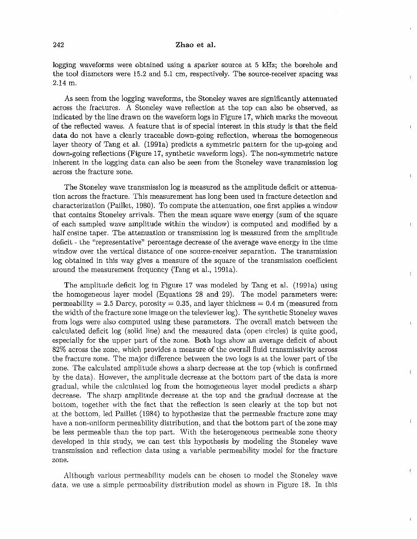
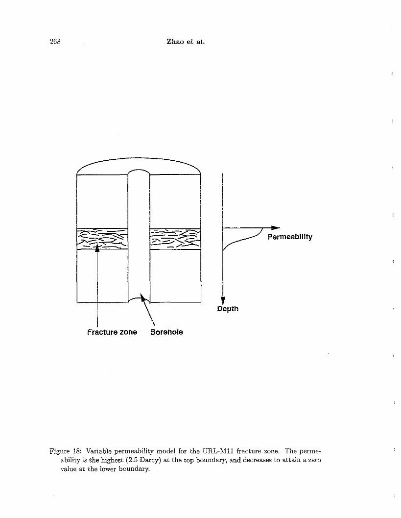
Although various permeability models can be chosen to model the Stoneley wavedata, we use a simple permeability distribution model as shown in Figure 18. In this

Permeability Heterogeneity 243

model, the permeability is assumed to attain its maximum at the top boundary, andsmoothly varies to Zero at the bottom boundary z = L = 0.4 m. This variation is givenas k(z) = ko[l+cos(I;1r)] where ko is chosen by requiring that i fl k(z)dz = 2.5 Darcy,which gives ko = 2.5 Darcy. In this way, the total fluid transmissivity of the fracturezone remains the same as the homogeneous layer model. The top boundary has asharp permeability contrast while the bottom boundary has no permeability contrast(Figure 18). In our numerical modeling, the other parameters used are the same as inthe homogeneous layer model. In addition, because of the pressure of the logging tool,

we use an effective borehole radius calculated using Ii. = JR2 - R't"oz.

For the permeability model in Figure 18, two numerical modeling experiments Wereperformed. In the first experiment, the incident Stoneley wave approaches the heteroge­neous zone from the bottom boundary (z = L) where there is no permeability contrast.This experiment is performed to simulate the logging operation of the acoustic loggingtool that is being pulled towards the fracture zone from below the zone. For the secondexperiment, we let the incident Stoneley wave approach the model from the top bound­ary (z = 0), where there is a sharp permeability contrast. This experiment is performedto simulate the acoustic logging tool that has just passed through the fracture zoneand is being pulled away from the zone. The downgoing Stoneley wave from the sourCewill interact with the fracture zone and the resulting reflection will be recorded by thereceiver.

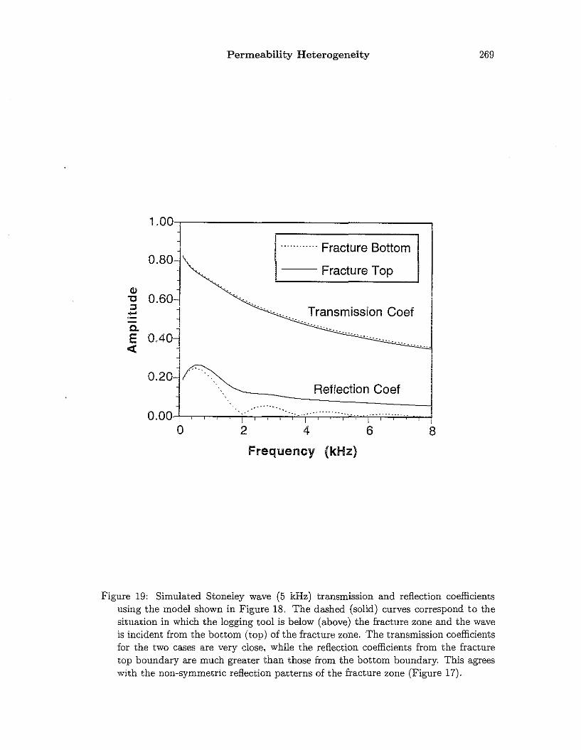
Figure 19 shows the calculated transmission and reflection coefficients for the two nu­merical modeling experiments in the frequency range of 0 ~ 8 kHz. The transmission co­efficients for the two experiments are very close and are around the value of 0.43 at about5 kHz. This will produce an amplitude deficit value of about (1-0.432) x 100% "" 0.82%,in excellent agreement with the measured value on the amplitude log. However, the re­flection coefficients for the two experiments differ greatly at higher frequencies, althoughthey approach each other towards the zero frequency (this suggests that the reflectiondata of very low frequency tube waVeS is not sensitive to the structure of the permeablezone, the same as shown in Fil,'1lres 9, 11, and 13). For the Stoneley wave approach­ing the top boundary of the fracture zone (sharp permeability contrast boundary), thereflection coefficient is about 0.1, which is about the same order of magnitude as theobserved reflected Stoneley wave amplitude shown in Figure 17. For the Stoneley waveapproaching the bottom boundary (zero permeability contrast boundary), the reflectioncoefficient value around 5 kHz is only about 0.02. Given the noise level in the measuredStoneley waveform data in Figure 17, reflected waves with such a small amplitude can­not be visually identified. Thus, the variable permeability model shown in Figure 18can model the reflection data very well.

To model the transmission data, we again need to use the finite difference methodand the propagator matrix formulation result given in Equation (24). When the receiverof the logging tool enters the fracture zone (source below receiver), the Stoneley waveis attenuated because of the propagation loss due to permeability. This amplitudeloss can be modeled by computing the Stoneley wave amplitude reduction from thebottom boundary to the receiver (assuming wave incidence from the bottom). In thisway, amplitude loss as a function of the receiver location can be modeled. Similarly,when the source enters the permeable zone (receiver above the zone), the Stoneley

244 Zhao at at

wave amplitude vs. source location can be simulated in a similar way (assuming waveincidence from the top boundary using reciprocity).

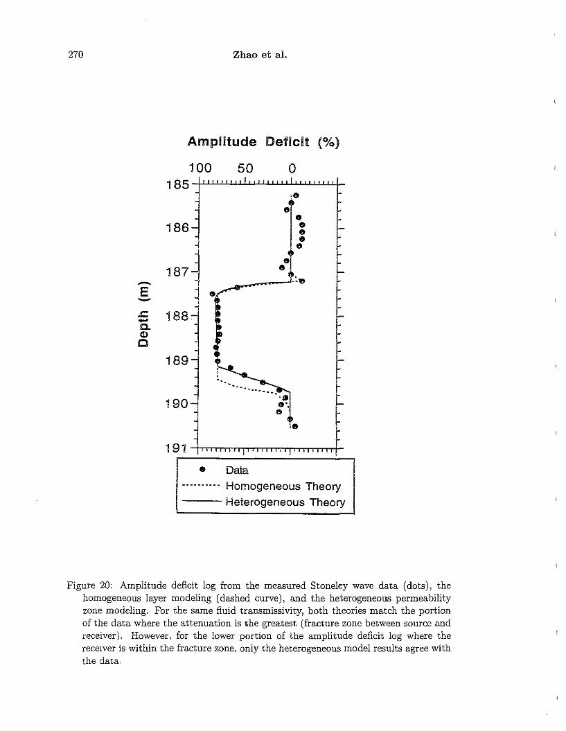
We again use the same variable permeability model shown in Figure 18. The simu­lated amplitude log (solid curve) for the permeability model in Figure 18 is plotted inFigure 20 with the measured amplitude log (dots) and the homogeneous layer modelresult (dashed curve). The homogeneous model results of Tang et al. (1991a) weremeasured from the synthetic seismograms shown in Figure 17 and were, therefore, ableto model the small amplitude increase due to the superposition of the incident andreflected waves at the top fracture zone boundary.

Although our simulation result is modeled in the frequency domain for the centralwave frequency of 5 kHz, the overall amplitude decrease across the fracture zone is notdifferent from the time domain measurement of the waveforms. The major improvementby our heterogeneous permeability model is at the lower portion of the amplitude deficitlog. Both the numerical result and the data show the same gradual change of amplitudewhen the receiver enters the fracture zone from the bottom boundary, while the homo­geneous model result shows the same sharp amplitude change as at the top boundary.Therefore, by using the variable permeability model, we successfully explain that thegradual amplitude change at the lower boundary is due to the small permeability forthe lower portion of the zone as compared to the upper portion. Thus, in additionto the agreement for the reflection data, the excellent agreement between theory anddata for the transmission data again supports the interpretation of the fracture zonepermeability distribution, as given by the variable permeability models (Figure 18).

The numerical modeling results confirm the hypothesis that the bottom part ofthe URL Mll well fracture zone is less permeable than the top part. This examplealso demonstrates how the numerical modeling approach can be used to assess thepermeability heterogeneities of borehole permeability heterogeneity from logging data.

CONCLUSIONS

An effective numerical analysis method has been developed to handle Stoneley wavepropagation through borehole heterogeneities. This technique is based on finite differ­ence modeling of dynamic fluid flow in a heterogeneous formation and the propagationmatrix method for wave propagation in a 1-D heterogeneous medium.

This technique can be used to calculate the effective Stoneley wave attenuationand velocity dispersion if the wave propagation distance is within the heterogeneousformation. When the heterogeneity variation is confined to a zone whose thickness issmall compared to the propagation distance, the technique can be used to calculate theStoneley wave transmission across the permeable zone and the reflection from the zone.

For continuous permeability variations, the cumulative Stoneley wave attenuationand veiocity dispersion can be weli described by a homogeneous permeability modelhavmg the average properties of the heterogeneous medium. For discontinuous varia­tIOns, sIgnificant deviation from the homogeneous model results exists only when the

Permeability Heterogeneity' 245

media has high permeability. The numerical modeling results demonstrate that, formost situations (low to medium permeability), the homogeneous model theory can bereliably used to obtain average permeability of a heterogeneous permeable formation.

For Stoneley wave transmission and reflection at a heterogeneous permeable struc­ture, the transmitted wave amplitude is controlled by the overall fluid transmissivity ofthe structure, although some discrepancy may arise depending on the structure of theheterogeneities. Reflection, on the other hand, is most sensitive to the structure of theheterogeneities. However, at very low frequencies, both transmission and reflection arecontrolled by the overall fluid transmissivity of the structure, irrespective of the distri­bution of heterogeneities within the structure. This shows that the low frequency tubewave can be used as an effective means to measure fluid transmissivity of the permeablestructure. The Stoneley wave reflection at higher frequencies can be used to detectheterogeneity variation within the structure.

The numerical modeling results have been verified by both laboratory experimentaldata and field acoustic logging data. Thus, for problems concerning acoustic logging inheterogeneous porous formations, the numerical method can be effectively used to helpdetermine formation permeability heterogeneities and their fluid transmissivity.

ACKNOWLEDGEMENTS

This research was supported by the Borehole Acoustics and Logging Consortium atM.LT. and by Department of Energy Grant DE-FG02-86ERI3636.

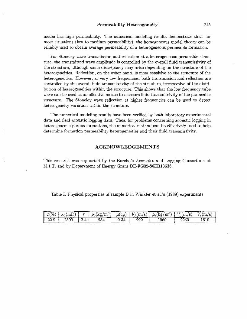
Table L Physical properties of sample B in Winkler et al.'s (1989) experiments

II <1>(%) l<o(mD) I T po(kg/m") I ",(cp) Vf(m/s) I Pe(kg/m") I 1/;,(m/s) Vs(m/s)II 22.9 2300 I 2.4 934 i 9.34 999 ! 1960 ! 2930 1610

246 Zhao et al.

APPENDIX

Finite Difference Solution of Dynamic Fluid Flow in (r, z) Coordinates

In borehole awustic logging in formations whose heterogeneity variation is in theradial (r) and vertical (z) directions, the (r, z) coordinates finite difference scheme isused to solve for the fluid flow in the heterogeneous medium. For the cylindrical system,the governing equation IS given by Equation (9):

(Ro < r < Rand 0 < z < L)

o ( OP) a(r,z) op 0 ( OP)or a(r, z) or + r or + OZ a(r, z) oz + iwp=O (A.l)

where Ra is the borehole radius, R is a large radial distance (R » Ra) at which pis effectively zero, and z = 0 and z = L represent the lower and upper boundaries ofthe heterogeneous formation, respectively. Equation(A.l) can be non-dimensionalizedto become (see Zhao et aI., 1993)

o I ,OP) . R-Ra ,op (R-Ra)2 0 (,ap) .ar' ~a or' + Ra + (R _ Ra)r,a fJr' + £2 fJz' a fJz' + ~(3p = 0

where

(A.2)

(A.3)I(r,z)

a' = ----------'-'--'-;Tn---------. 1/2 '

[1- ~rKmaxl(r,z)pr$] - irl<maxl(r,z)Pd;

is the non-dimensionalized dynamic fluid diffusivity, I(r, z) = I«r, z) is the dimension-I<max

less permeability distribution in the (r,z) coordinated, I<max being the maximum per-

meability in the model, and (3 = w(R - Ra)2/ao , where ao = I<m;'¢Kt is the maximum

fluid diffusivity in the model. The dimensionless spatial variables are given by

Zi =

r- RoR Ro

z/L

(0 < r l < 1)

(0 < z' < 1)

Solution of Equation (A.2) can be obtained as the steady-state solution of the fol­lowing equation,

fp= : (A.4)

where fp is the left hand side of Equation (A.2), and t' is a dimensionless time. Thesteady-state solution is found by employing a stable iterative procedure using the ADImethod. The variables r', z', and t' are discretized as

{

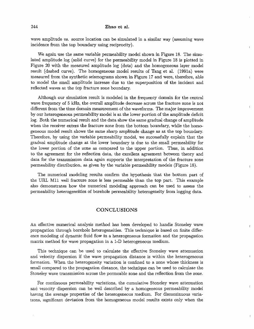
r' = i£:"r'z' = jt1z't' = nt1t'

i = 0, 1. 2, . . " \ Ij = 0, 1,2,"',Jn = 0, 1~ 2, ... 1 N

t1r' = 1/1t1z1 = I/J (A.5)

Permeability Heterogeneity

where ,6.t! can be chosen as J(,6.r,2 + ,6.z'2)/2.

247

To use the ADI method to solve Equation (AA), we re-write this equation in theform of

where,

iA iJ ( ,iJp ) R-R.D ,iJP'(3

IP = a:? a a:? + R.D + (R _ R.D)r' a a:? + t P

_ (R - R.D)2 iJp ( f iJp)A2P - L2 8l a 8l .

The ADI finite difference form of Equation (A.B) is

(bit' ) - / bit' )1- ZAlh pn+I/2 = (I + ZA2h pn

(I bit' A ) n+1 (- bit' A ) n+I/2--2hP =l+-IhP2 2

where Alh and A2h are finite difference operators:

1 [ (1),6.r,2 (Bi.j - Di,j)Pi-I,j - (Bi,j + B i+1,j - Di,j

-i(3bir'2)pi,j + BHI,jPHI,j]

(2) 1= Di,j biz,2 [Ci,jPi,j-I - (Ci,j + Ci.j-I)Pi,) + Ci,j+IPi,j+I]

whereAi,j = a~,j

B- _ = Ai,; + Ai-I,!1.,) 2

C. _ Ai,i + Ai,i-It,} 2

D(I) = (R - R o)Bi,i,6.r'',) [R.D + (R - R.D)(r:,j + r:_I,j)/2]

D(2) = (R - R.D)2\. t,) L2

Therefore, the finite difference form of Equations (A.lO) and (A.ll) is

( D (I») n+I/2 'l _ ( (1)-iLl Bi,j - i,j Pi-I,j + 1 + iLl Bi,j + BH1,j - Di,j

'(3,6. '2)] n+I/2 B n+l/2-~ r Pi,} - f.Ll i+l,jPi+l,J

- D(2) n [1 (C C ') D(2)] n D(2)C n- J.L2 i,i Pi,j-l + - i,j + i,j+l fL2 i,j Pi,i + /-L2 i,i i,j+lPi,j+l

D (2)C n+l 'l- - D(2)(C C )1 n+1 D(2)C n+1-iL2 i,j i,jPi,j-! + 1 + iL2 i,j i,) + "j+1" Pi,j - iL2 i,j i,j+IPi,j+I- (. (1)) n+I/2 r ( (1)- /1-1 B,,) - Di,) Pi-I,) + 1 - /1-1 , B,,) -j- Bi+I,) - Di,j

'/3 A '2)] n+I/2 B - n+l/2-1. uT Pi,} + I-tl i+l,JPi+l,J

(A.6)

(A.7)

(A.8)

(A.9)

(A.I0)

(A.ll)

(A.12)

(A.13)

(A.14)

248

where

!J.t'/11 = ? A '2

~l.J.r

Zhao et al.

and!J.t'

/12 =?A ,2'~l.J.z

The boundary conditions for the problem are given in Equations (11), (12), and(13), which in the finite difference form, are given by

and

{p(O, j) =:.poexp{ike!J.z'j}p(R,J) - 0 .

{p(i, 0) = p(i, 1)p(i, J - 1) = p(i, J)

(0 < j < J)

(0 < i < I) .

(A.15)

(A.16)

The finite difference Equations (A.13) and (A.14), together with the boundary con­ditions, can be solved using Thomas algorithm (see Zhao et al., 1993 and Ferziger,1980).

Permeability Heterogeneity

REFERENCES

249

Aki, K., and P.G. Richards, 1990, Quantitative Seismology, W.H. Freeman and Co.,New York.

Cheng, C.H., and M.N. Toksiiz, 1981, Elastic wave propagation in a fluid-filled boreholeand synthetic acoustic logs, Geophysics, 46, 1042-1053.

Ferziger, J.H., 1981, Numerical Methods for Engineering Applications, John Wiley &Sons, Inc., New York.

Giiler, F., and M.N. Toksiiz, 1987, Ultrasonic laboratory study of full waveform acousticlogs in boreholes with fractures, M.l. T. Full Waveform Acoustic Logging ConsortiumAnnual Repori.

Hornby, RE., D.L. Johnson, K.H. Winkler, and R.A. Plumb, 1989, Fracture evaluationusing reflected Stoneley-wave arrivals, Geophysics, 54, 1274-1288.

Johnson, D.L., J. Koplik, and R. Dashen, 1987, Theory of dynamic permeability andtortuosity in fluid-saturated porous media. J. Fluid Mech., 176, 379-400.

Kostek, S., 1991, Borehole acoustic wave propagation in the presence of fractures: A fi­nite difference approach, SEG 61st Ann. Inti. Mtg. fj Expo. Expanded Abst. Houston,Texas.

Kostek, S., 1990, Modeling of elastic wave propagation in a fluid-filled borehole excitedby a piezoelectric transducer, Masters thesis, M.LT., Cambridge.

Norris, A.N., 1989, Stoneley-wave attenuation and dispersion in permeable formations,Geophys,cs, 54, 330-341.

Paillet, F.L., 1980, Acoustic propagation in the vicinity of fractures which intersect afluid-filled borehole, Trans., Soc. Prof. Well Log Analysts, 21st Ann. Symp., paperDD.

Paillet, F.L., 1984, Field test of a low-frequency sparker source for acoustic waveformlogging, M.I. T. Full Waveform Acoustic Loggmg Consortium Annual Repori, 207­228.

Tang, X.M., and C.H. Cheng, 1988, Wave propagation in a fluid-filled fracture: Anexperimental study, Geophys. Res. Ltt., 15, 1463-1466.

Tang, X.M., C.H. Cheng, and F.L. Paillet, 1991a, Modeling Stoneley wave Propagationacross in-situ fractures, Trans. 36th Soc. Prof. Well Log Analysis, Paper GG.

Tang, X.M., C.H. Cheng, and M.N. Toksiiz, 1991b, Danymic permeability and doreholeStoneley waves: A simplified Blot-Rosenbaum model, J. Acous. Soc. Am., gO, 1632­1646.

Tang, X.M., and C.H. Cheng, 1993, Borehole Stoneley wave propagation across hetero­geneous and permeable structures, Geophys,cal Prospecting, 41, 165-187.

250 Zhao et aI.

Winkler, K.W., H.L. Liu, and D.L. Johnson, 1989, Permeability and borehole Stoneleywaves: Comparison between experiment and theory, Geophysics, 54,66-75.

Zhao, X.M., and M.N. Toks6z, 1991, Modeling fluid flow in heterogeneous and anisotropicporous media, M.l.T. Full Waveform Acoustic Logging Consortium, 245-270.

Zhao, X.M., C.H. Cheng., X.M. Tang, and M.N. Toks6z, 1992, Dynamic fluid flowin heterogeneous porous media and through a single fracture with rough surfaces,M.l. T. Borehole Acoustics and Logging Consortium, 157-178.

Zhao, X.M., M.N. Toks6z, and C.H. Cheng, 1993, Stoneley wave propagation in het­erogeneous porous formations, M.l. T. Borehole Acoustic and Logging Consortium,43-78.

Permeability Heterogeneity

1400L,

1350 t .... .....

>III

1300 t-E~,.,

1250 (a).<;::u0Qj 1200> 1-- Finite Difference

1150 ........... Analytical

11000 2 3 4 5

Frequency (kHz)

251

-- Finite Difference........... Analytical

0.5

"0.4

-::.c: 0.30:;::.," 0.2c:.&

~-<t0.1

o ~a 2 3 4 5

(b)

Frequency (kHz)

Figure 1: Comparison between analytical (dashed curves) and finite difference (solidcurves) results: (a) Stoneley wave velocity, (b) Stoneley wave attenuation.

252 Zhao et al.

0.0 2.0

Figure 2: Random permeability model (left) generated using 2-D Gaussian correlationfunction and simulated pore fluid pressure contour (nght) in the formation for a100 Hz Stoneley wave. The model dimensions are: 10 m in the z-direction and 1 mm the r-direction. Permeability ranges from a- .2 Darcy.

Permeability Heterogeneity 253

r

0.00 2.00

Figure 3, I-D permeability model (iett) with a Gaussian correlation function and simu­lated pore fluid pressure contour (right) for a 100 Hz Stoneley wave. Model dimen­sions are the same as in Figure 2.

254

r

Zhao et al.

0.00 2.00

Figure 4: Cyclic permeability model (left) and the simulated pore pressure contour(right) for a 100 Hz Stoneley wave. Model dimensions are the same as in Figure 2.

Permeability Heterogeneity

1400

.-...-'".. -,.

1350

~ 1300 r /~~ /

.§. .' "• 0,..1250

/.r-(a)- /''0

0 --Homogeneousa; 1200 ----- Gaussian> I I·········· l-D Gaussian1150 I _ .•• - Poisson

1100

0 i 2 3 4 5

Frequency (kHz)

0.5

--Homogeneous

a- 004 - - - - - - Gaussian..... ........... 1-D Gaussian~~ _ ... - Poisson0.3c0

(b);;::\U= 0.2 r~,c.,

.~- '~:r ....:..-<C0.1 f '.....::~.~~~,,~~-- ---

-···_· ..~7..==:--..==:'".._.0

0 1 2 3 4 5

Frequency (kHz)

255

Figure 5: Stoneley wave phase velocity (a) and attenuation (b) curves for different het­erogeneous permeability models. The average permeability of the models is 1 Darcy.

256 Zhao et aL

1400

--.~.- ...1300

~ 1200.!!!E- 1100>0- (a)-'u 1000 -- Homogeneous0Gi ------ Gaussian> 900 ........... 1-D Gaussian

800 - ... - Poisson

7000 1 2 3 4 5

Frequency (kHz)

-- Homogeneous------ Gaussian........... 1-D Gaussian_ ... - Poisson

co:;:;.."c.,::::<

1

0.8

0.6

0.4

0.2 ~

, ,.,~

.,.~

\".< ,", ...; ..

" :-'. -- ...- ...~-:----1-"--'''-'''-...-

(b)

51 2 3 4

Frequency (kHz)

o L.....~""""'-'c.......~..-J.~~"-'-~~'-'-~~...J

o

Figure 6; Stoneley wave phase velocity (a) and attenuation (b) curves for different het­erogeneous permeability models. The average permeability of the models is 10 Darcy.

Permeability Heterogeneity

1.00

Finite Difference0.80 ......... Analytical

(1l 0.60v Transmission Coef:;,- ~-~-------- -----

a. 0.40E«

0.20Reflection Coef

0.000 1 2 3 4 5 6

Frequency (kHz)

257

Figure 7: Testing the results of numerical modeling of Stoneley wave propagation acrossa permeable zone (solid curves) using the analytical solution results (dashed curves).

258 Zhao et al.

~ - ----.,

li5

\Borehole

Depth

I

I

Permeability

Figure 8: Double permeability layer model for modeling Stoneley wave propagation.Two layers of 10 Darcy permeability and 0.15 m thickness are separated by a non­permeable formation of 0.2 m thicl<.

Permeability Heterogeneity 259

Transmission Coef

-- Double layer--- .. _.. _-- Single layer

1.00

0.80

Ql

" 0.60:::l:=a.E DAD -j<t

~0.2°1

j0.00 i

0I2

, i4

I.:;ti~

Frequency (kHz)

Figure 9: Stoneley wave transmission and reflection coefficients (solid curves) for thedouble layer model shown in Figure 8. For comparison, the results for a homogeneouslayer with cumulative thickness of 0.3 m and 10 Darcy permeability are also shown(dashed curves). The two results agree only in the low frequency limit.

260 Zhao et aI.

Permeability

Depth

BoreholeFrJcture zone

....--.... ~

I

II ...10..

'\

Figure 10: Multiple layer permeable zone model. The thickness and average permeabil­ity of the zone are 0.4 m and 10 Darcy, respectively.

CD"C:::l.....-0..E<t

1.00

0.80

0.60

0.40

0.20

Permeability Heterogeneity

-- Multi-Frc Zone........... Homogeneous Zone

Transmission Coef

'" -.

Reflection Coef

261

o 2 4

Frequency6

(kHz)8

Figure 11: Stoneley wave transmission and reflection coefficients for the multiple layerzone model (solid curves) shown in Figure 10. For comparison, the results for ahomogeneous zone of thickness 0.4 m and permeability 10 Darcy are also shown(dashed curves).

262

............." ....................................: '/ 'J ............................. ' ..

II

Fracture zone

Zhao et al.

.....:; .::. ;, \:0.."'··..1+--1 Permeability. ..

. ',"

.. ..

Depth

Borehole

Figure 12: Permeability zone model with random permeability variation along the bore­hole aXial direction. The variation is characterized by Gaussian correlation function.The average permeability of the mode! is 10 Darcy.

Permeability Heterogeneity 263

Figure 13: Stoneley wave transmission and reflection coefficients (solid curves) for therandom permeability model of Figure 12. The results for a uniform permeability(10 Darcy) layer are also shown (dashed curves).

266 Zhao et aI.

1000

950 eJ'¥ --- - - ......~

~..!!! 900E~

j>- 850 (a)-'u0Qi 800 :.,

------Uniform> .I• --Poisson

750 •· .....•.... Data·,·700

a 20 40 60 80 100

Frequency (kHz)

0.8 ,,0.7 , -----·Uniform,,

--Poisson~ 0.6" .......... Data-~~ 0.5 .."<:

0 0.4 ~ (b):::'" ~::

0.3 i<: Iill I- ,- 0.2 i:« I

o.~ 1 :::"i:O~~::--:;~;;:- .-.~i, I,

0 20 40 60 80 100

Frequency (kHz)

Figure 16: Comparison of the experimental Stoneiey wave veiocity (a) and attenuation(b) data (dots) with the theoretical modeiing resuits (soUd curves) using the dis­continuous permeability iayer modeL There is an excellent agreement between dataand theory for both veiocity and attenuation.

Permeability Heterogeneity

TUBE-WAVE AITENUATION AND REFLECTION

MODEL

Lt:.:; \J'

267

1.0 2.0 3.0 ~.O 0 1.0 2.0 3.0 40 5.0

TIME. IN MP.... LlSECONOS

Figure 17: Stoneley waveforms, amplitude log, and televiewer log for the URL-Mll wellaround 188 m (After Paillet, 1984), The theoretical modeling results of Tang et aL(1991a) are also shown in this figure,

268 Zhao et al.

Permeability

Depth

BoreholeI

Fracture zone

~ - ~

I I-:2'~ -- i=----:i >-~;;::::.~-...;::,.

::;:-...-~..:.:-~:- c:" _.....

II

~

, '\

Figure 18: Variable permeability model for the URL-Mll fracture zone. The perme­ability is the highest (2.5 Darcy) at the tOP boundary, and decreases to attain a zerovalue at the lower boundary.

Permeability Heterogeneity

1.00,-r---------------,

269

0.80............ Fracture Bottom

Fracture Top

CIl"0 0.60-jE ~ Transmission Coef~ ~ " ..

~00401... .020]~::Refl~~t;onCoef

0.00 ~" : . I' '·'1-··' .. ·.. ·02468

Frequency (kHz)

Figure 19: Simulated Stoneley wave (5 kHz) transmission and reflection coefficientsusing the model shown in Figure 18. The dashed (solid) curves correspond to thesituation in which the logging tool is below (above) the fracture zone and the waveis incident from the bottom (top) of the fracture zone. The transmission coefficientsfor the two cases are very dose. while the reflection coefficients from the fracturetop boundary are much greater than those from the bottom boundary. This agreeswith the non-symmetric reflection patterns of the fracture zone (Figure 17).

.,

270 Zhao et al.

Amplitude Deficit (%)

100 50 0185

,e

186~e .,.,

0

~.,

.e.,187 ct

- ·:eE .,-J:: 188-c.(1)

C

189

Data

Homogeneous Theory

--- Heterogeneous Theory

Figure 20: Amplitude deficit log from the measured Stoneley wave data (dots), thehomogeneous layer modeling (dashed curve), and the heterogeneous permeabilityzone modeling. For the same fluid transmissivity, both theories match the portionof the data where the attenuation is the greatest (fracture zone between source andreceiver). However, for the iower portion of the ampiitude deficit log where thereceIver is within the fracture zone, only the heterogeneous model results agree withthe data.