strain fields in crystalline solidscore.ac.uk/download/pdf/11478935.pdf · strain fields in...
TRANSCRIPT

Strain Fields in Crystalline SolidsPrediction and Measurement of X-Ray Diffraction Patterns
and Electron Diffraction-Contrast Images
Proefschrift
ter verkrijging van de graad van doctoraan de Technische Universiteit Delft,
op gezag van de Rector Magnificus prof.ir. K.F. Wakker,in het openbaar te verdedigen ten overstaan van een commissie,
door het College voor Promoties aangewezen,op dinsdag 16 mei 2000 te 16.00 uur
door
Teunis Cornelis BOR
materiaalkundig ingenieurgeboren te Schoonrewoerd

Dit proefschrift is goedgekeurd door de promotoren:
Prof.dr.ir. E.J. MittemeijerProf.dr.ir. E. van der Giessen
Samenstelling promotiecommissie:
Rector Magnificus voorzitterProf.dr.ir. E.J. Mittemeijer Technische Universiteit Delft, promotorProf.dr.ir. E. van der Giessen Technische Universiteit Delft, promotorProf.dr.ir. P. van Houtte Katholieke Universiteit Leuven, BelgiëProf.dr. J.Th.M. de Hosson Rijksuniversiteit GroningenProf.dr. H.W. Zandbergen Technische Universiteit DelftDr. I. Groma Eötvos University Budapest, HongarijeDr.ir. R. Delhez Technische Universiteit Delft
Dr.ir. R. Delhez en dr.ir. Th.H. de Keijser hebben als begeleider in belangrijke mateaan de totstandkoming van het proefschrift bijgedragen.
The work described in this thesis was made possible by financial support from theFoundation for Fundamental Research of Matter (FOM) and partly by financialsupport from the Netherlands Technology Foundation (STW).

Contents
1. General Introduction 1
2. X-Ray Diffraction Line Shift and Broadening of Precipitating Alloys;
Part I: Model Description and Study of "Size" Broadening Effects 7
1. Introduction ...................................................................................................... 7
2. The line-profile simulation model .................................................................... 9
2.1. The strain field of the particle-arrangement unit cell ................................ 9
2.2. Method of line-profile calculations ......................................................... 12
2.2.1. Sampling of displacement field ..................................................... 12
2.2.2. Intensity distribution of a single crystal......................................... 12
2.2.3. Intensity distribution of a polycrystalline powder; sampling in
reciprocal space.............................................................................. 16
2.2.4. Computing time considerations..................................................... 16
2.3. Characterization of line profiles .............................................................. 17
3. The interpretation of "size broadening".......................................................... 18
3.1. Introduction ............................................................................................. 18
3.2. Centroid and variance; numerical results ................................................ 18
3.3. Relation between particle fraction and line width ................................... 20
3.4. Relation between particle number density and line width;
variance-range plots................................................................................. 22
3.5. Effect of particle clustering ..................................................................... 25
4. "Size-strain separation" .................................................................................. 27
5. Conclusions .................................................................................................... 28
Appendix A: Interpolation of displacement field within an element ................... 29
Appendix B: Calculation of the structure factor using the Fast Fourier
Transform algorithm ...................................................................... 30
Appendix C: Influence of the rotation procedure on the centroid and variance
of the {hk} powder diffraction line profile .................................... 36
Appendix D: Calculation of the size Fourier coefficients of a p.a.-unit cell
containing clustered particles......................................................... 38
References ........................................................................................................... 40
3. X-Ray Diffraction Line Shift and Broadening of Precipitating Alloys;
Part II: Study of "Strain" Broadening Effects 41
1. Introduction .................................................................................................... 41
2. Basis of micromechanical and diffraction calculations .................................. 42
3. Characterization of strain fields and line profiles........................................... 43

4. Analysis of misfit-strain fields ....................................................................... 45
4.1. Role of particle fraction; orientation dependence of strain parameters ... 45
4.2. Role of particle/matrix misfit; scaling properties .................................... 50
4.3. Role of particle clustering........................................................................ 50
5. Line-profile calculations................................................................................. 53
5.1. Role of mechanical properties ................................................................. 53
5.2. Role of particle fraction........................................................................... 56
5.3. Role of p.a.-unit cell size......................................................................... 56
5.4. Role of clustering..................................................................................... 59
5.5. Concluding remarks on line profile centroid and variance...................... 59
6. Conclusions .................................................................................................... 62
Appendix A: Directional independence of mean matrix strain ⟨ ⟩ehk p.a. ............. 63
Appendix B: Strain field for circular inclusion in circular matrix ....................... 65
References ........................................................................................................... 66
4. Diffraction Contrast Analysis of Misfit Strains around Inclusions
in a Matrix; VN Particles in αα-Fe 67
1. Introduction .................................................................................................... 68
2. Calculated BF and DF diffraction contrast images......................................... 69
2.1. Theoretical background ........................................................................... 69
2.1.1. Dynamical theory of electron diffraction....................................... 69
2.1.2. Displacement field of a misfitting particle .................................... 71
2.1.3. Procedures of strain field contrast image calculation.................... 72
2.2. Results of BF and DF diffraction-contrast calculations .......................... 73
2.2.1. Characterization of the contrast image; the image width .............. 73
2.2.2. Parameters determining the image width ...................................... 74
2.2.2.1. Foil thickness .................................................................... 75
2.2.2.2. Particle radius.................................................................... 76
2.2.2.3. Particle Burgers vector...................................................... 76
2.2.2.4. Particle position ................................................................ 78
2.2.2.5. Neighbouring particle; overlapping strain fields............... 79
3. Specimen preparation ..................................................................................... 81
4. Fitting calculated diffraction contrast images to experimental diffraction
contrast images of VN in α-Fe ....................................................................... 83
4.1. Selection of experimental diffraction contrast images of misfitting
particles ................................................................................................... 83
4.2. Fitting of particle Burgers vector and foil thickness ............................... 87
5. Additional results and discussion ................................................................... 93

5.1. Particle size and visibility of strain contrast ............................................ 93
5.2. Platelet thickness ..................................................................................... 93
5.3. Occurrence of misfit dislocations; lattice plane imaging ........................ 94
5.4. X-ray diffraction line-shift and -broadening............................................ 96
6. Conclusions .................................................................................................... 99
Appendix: Rearrangement of Howie-Whelan equations for a four beam case.. 100
References ......................................................................................................... 102
5. A Method to Determine the Volume Fraction of a Separate Component in a
Diffracting Volume 105
1. Introduction .................................................................................................. 105
2. Theoretical basis ........................................................................................... 106
3. Experimental................................................................................................. 107
4. Results and discussion.................................................................................. 108
5. Conclusions .................................................................................................. 112
References ......................................................................................................... 112
6. Analysis of Ball Milled Mo Powder using X-ray Diffraction 115
1. Introduction .................................................................................................. 115
2. Theoretical basis ........................................................................................... 116
2.1. Description of diffraction-line profiles in real space and Fourier space 116
2.2. Deconvolution with prior normalization ............................................... 118
2.3. Deconvolution without prior normalization .......................................... 119
3. Experimental................................................................................................. 120
4. Evaluation of X-ray diffraction data............................................................. 122
5. Results and discussion.................................................................................. 125
5.1. Morphology of ball milled powder........................................................ 125
5.2. Volume fraction of undeformed powder particles in ball milled
powder ................................................................................................... 127
5.3. Deformation texture............................................................................... 129
5.4. Evolution of structural imperfection...................................................... 131
5.4.1. Integral breadth as function of ball milling time ......................... 131
5.4.2. Integral breadth as function of diffraction-vector length............. 132
5.5. Interpretation of microstrain; determination of dislocation density ...... 136
6. Conclusions .................................................................................................. 141
Appendix: Relation between THKL and αHKL ...................................................... 142
References ......................................................................................................... 143

Summary 145
Samenvatting 149
Nawoord 153
Curriculum Vitae 155
Chapter 1
General introduction
Nowadays, the search for new, better, stronger and lighter materials has become a
field of large interest, both from a scientific and an economical point of view [1-3].
Development of new and/or improved materials is considered to be essential in, for
example, semi-conductor, aircraft and space industries [3]. Such a development
requires fundamental knowledge of materials behaviour on all relevant length scales,
such as the (mis)arrangement of atoms at a nanometer scale and the orientation,
distribution and behaviour of grains and grain boundaries at the micrometer scale in
order to understand and predict the behaviour of macro-sized products [4].
The prediction of the overall (mechanical) behaviour is possible using
micromechanics [5]. A small volume, which is representative of the microstructure of
the material, is used to model and calculate the materials behaviour on a local
(mesoscopic) scale using continuum mechanics. Subsequently, the behaviour of the
representative element is used to calculate the overall materials properties. In this
respect characterization of materials through experimental techniques, such as light
microscopy, X-ray diffraction (XRD), Scanning Electron Microscopy (SEM) and
Transmission Electron Microscopy (TEM) [6], plays an essential role. These
techniques do not only contribute to the qualitative, theoretical understanding of
materials behaviour, but they also serve as tools to obtain quantitative input for
materials modelling. It is the combination of the powers of micromechanics and X-ray
diffraction for the understanding and prediction of materials properties and behaviour
that forms the incentive for this thesis.
Scope of thesis
The main part of this thesis is concerned with X-ray powder diffraction, i.e. the line
profile analysis of polycrystalline specimens for the characterization and investigation
of materials. Powder diffraction is non-destructive in nature and enables structural
information to be obtained over a moderately large (sample) volume (~1 mm3) [7]. A
powder diffraction-line profile contains a wealth of information yielding many
characteristics from the same measured data (of which); some characteristics cannot
be obtained from other analysis methods [8, 9, 10].
The positions of the line profiles enable phase and structure identification and
the determination of (macro) strain (i.e. average strain over the length scale of
diffracting crystallites). From the integrated intensities, the amount of phases present

2 Chapter 1
can be determined and preferential orientation of crystals (i.e. texture) can be
established. The analysis of the shape (broadening) of the line profiles enables the
determination of the (finite) size of the diffracting crystallites, of the presence of all
kinds of lattice imperfections that cause microstrains (i.e. strains varying over the
length scale of the diffracting crystallites), of stacking and twin faults and of
compositional inhomogeneities.
Examples of lattice imperfections causing microstrains are dislocations and
(small) misfitting particles/precipitates, see Fig. 1. These imperfections cause the
atomic lattice to be deformed, i.e. locally the atomic spacing is increased or decreased.
In the absence of such lattice imperfections (and employing a perfect measurement
instrument with a single wavelength) the XRD line profiles would resemble sharp,
delta-function like, peaks. The peak position follows directly from the use of Bragg's
law, which relates the lattice spacing to the diffraction angle(s). Hence, it is
understandable that lattice imperfections induce line broadening: small variations in
the (local) atomic spacing correspondingly cause small variations in the diffraction
angles.
Lattice imperfections have a large influence on the (mechanical and other)
properties of crystalline materials. The motion of dislocations facilitates the
deformation of crystalline materials and therefore, mechanical properties, such as the
hardness and the yield strength, are improved greatly by hindering the dislocation
motion [9]. One way to block or obstruct dislocation motion is the introduction of
small (nanometer sized), misfitting precipitates/particles in the (matrix) material.
Another way to impede dislocation motion reveals itself during (cold) deformation:
dislocations hinder each other, leading to a dramatic increase of the dislocation
density (strain hardening). Further, the presence of dislocations is important for the
recrystallisation behaviour of (deformed) materials [11].
From the above it follows that since the presence and properties of lattice
imperfections largely determine both (i) the behaviour and properties of materials and
(ii) the shift and broadening of XRD line profiles, a potential route to the direct
understanding of materials behaviour from the analysis of XRD line shift and
broadening is conceivable. Hence, it is important to establish sound relationships
between the line shift and broadening measured and the type and amounts of lattice
imperfections present.
However, the analysis of line broadening is not straightforward [7 - 10, 13].
Within a single specimen several types of lattice imperfections may occur and cause
line broadening (structural line broadening). Moreover, the measured line broadening
is augmented by additional broadening due to the measurement instrument and the
spectral distribution of the X-rays (instrumental line broadening) [9, 10], see Fig. 1.
General Introduction 3
Fortunately, the instrumental line broadening can be separated from the total line
broadening with the aid of a suitable reference specimen that is practically free of
lattice imperfections [9, 10].
In a line-broadening analysis the respective contributions of the sources of
structural line broadening are to be identified. With the aid of certain assumptions and
often using several orders of reflection, the structural broadening is usually separated
into a contribution due to size (the finite size of the diffracting crystallites) and a
contribution due to strain (including all microstrain sources). Examples of such size-
strain analysis methods are the Williamson-Hall analysis [14], the Warren-Averbach
analysis [9] and an alternative analysis by Van Berkum et al. [15]. Although these
types of analysis can be performed in a relatively straightforward manner and are
applicable independent of the types of lattice imperfections present, they suffer from
at least two drawbacks. Firstly, the assumptions underlying the methods are not
always verified or even correct, leading to unreliable outcomes [15], and secondly, the
interpretation of the size and strain contributions in terms of the microstructural
features (e.g. dislocations, precipitates) of the polycrystalline material considered is
very often difficult [15].
Recently a novel way of line-profile analysis has been proposed which is the
main theme of this thesis [16]. On the basis of an adequate physical/micromechanical
model of the lattice imperfections within a representative volume of the crystalline
material, XRD line profiles are calculated. The calculated line profiles are matched to
the experimental line profiles by changing (a limited number of) model parameters
that are directly related to the type and distribution of the lattice imperfections. In this
way the values of relevant physical parameters are determined directly. Evidently,
their accuracy/reliability depends upon the adequacy of the physical model.
In addition to a proper determination of the relevant physical parameters
another (fruitful) outcome of this methodology is the elimination of so-called
truncation errors. In diffraction-line broadening analysis, one practically never obtains
the full line profile due to overlap with line profiles of neighbouring reflections and
the presence of a background intensity. Each measurement of a line profile suffers
therefore from truncation both vertically (finite measurement range) and horizontally
(subtraction of background), which affects the results of all subsequent analysis [7, 9,
10, 17]. However, if an appropriate description of the structural broadening is
available and the instrumental line broadening is known, the entire diffraction-line
profile, or even the complete diffraction pattern, could be calculated and fitted at once.

4 Chapter 1
↓ ↑ ↓ ↑
log(
Inte
nsity
) (a
.u.)
150145140135130125º2θ
with particles
no particles
log(
Inte
nsity
) (a
.u.)
91898785º2θ
with dislocations
"no" dislocations
Fig. 1. Atomic representation of model materials containing misfitting particles (a) or (edge)
dislocations (b) for interpretation and generation (illustrated by the ↑ ↓ -symbols) of X-ray
diffraction-line profiles. The distortion of the lattice due to the strain fields of the lattice
imperfections cause broadening of the X-ray diffraction line profiles (structural broadening).
Examples of experimental line profiles are displayed for a VN precipitates containing α-Fe
matrix (c) (see also Chapter 4) and a cold deformed, ball milled, Mo powder (d) (see also
Chapters 5 and 6). The structural line broadenings are obtained by elimination of the line
broadenings in absence of lattice imperfections (instrumental line broadening).
(a) (b)
(c) (d)
General Introduction 5
The outcomes of the diffraction-line profile calculation and fitting
methodology must, of course, be verified. Even in the case of just a single solution for
the model parameters, the physical relevance of the micromechanical model must be
checked. In this respect the following sources of errors should be recognised. Firstly,
the measurement of experimental line profiles is always hindered by (counting)
statistical intensity variations. Secondly, a relatively simple micromechanical model
can describe the important features of the experimental material successfully, but it
will not be capable of capturing all details.
An obvious route to check the validity of the parameters determined from
XRD is to study the same material using a different experimental technique.
Transmission Electron Microscopy serves as an excellent candidate in this respect,
since it enables a detailed study of very small volumes containing the lattice
imperfections causing broadening of X-ray diffraction-line profiles [18].
Contents of thesis
This thesis contains three parts. In the first part, chapters II and III, the novel XRD
methodology is explained and studied in full detail for the case of misfitting
particles/precipitates in a matrix. Both the broadening due to finite size effects
(chapter II) and due to microstrains (chapter III) are considered and a simple method
of separating both broadenings is proposed. The broadening due to microstrains is
studied in two steps. First the relations between model parameters, such as the particle
size, the particle fraction, the particle-matrix misfit and the distribution of particles
within the matrix, and characteristic values of the strain within the matrix, such as the
mean strain and the root mean square strain, are investigated in detail. Subsequently,
the relations between the values that characterize the matrix strains and the shift and
width of calculated line profiles are analysed.
In the second part, chapter IV, a particle-matrix model system is studied using
Transmission Electron Microscopy to enable verification of the results of the
simulation methodology. A model system, consisting of an α-Fe matrix filled with
small, misfitting VN precipitates is studied in detail. A new method of determining
the particle-matrix misfit from TEM micrographs is proposed.
In the last part, attention is paid to ball milling/mechanical alloying [19]. In a
ball milling device, small amounts of elementary and/or alloyed powder particles can
be deformed severely using one or more vibrating balls. The deformation process
induces large numbers of lattice imperfections, such as dislocations and grain
boudaries. In chapters V and VI the first stages of the ball milling of elementary Mo
powder in a low-impact ball milling device are studied. Special attention is devoted to

6 Chapter 1
the determination of the fractions of powder particles that remain undeformed for
relatively short milling times.
references
[1] P. Ball, Made to Measure, New Materials for the 21st Century, Princeton University Press,
Princeton, New Yersey, 1997.
[2] M. Schwartz, Emerging Engineering Materials: Design, Processes, Applications,
Technomic Publishing Company, Inc., Lancaster, 1996.
[3] M.C. Flemings, Ann. Rev. Mater. Sci. 29 (1999), 1 - 23.
[4] E. Lifshin (ed.), Materials Science and Technology 2A, part I, Weinheim, 1992.
[5] S. Nemat-Nasser, M. Hori, Micromechanics: Overal Properties of Heterogeneous
Materials, Elsevier, Amsterdam, 1999.
[6] F.H. Chung, D.K. Smith, (eds), Industrial Applications of X-Ray Diffraction, Marcel
Dekker, Inc, New York, 2000.
[7] R. Delhez, Th.H. de Keijser, E.J. Mittemeijer, Fres. Z. Anal. Chem 312 (1982), 1 - 16.
[8] H.P. Klug, L.E. Alexander, X-Ray Diffraction Procedures, John Wiley, New York, 1974.
[9] B.E. Warren, X-ray Diffraction, Reading, Massachusetts: Addison-Wesley, 1969.
[10] R.L. Snyder, J. Fiala, H.J. Bunge, Defect and Microstructure Analysis by Diffraction,
Oxford University Press, New York, 1999.
[11] G.E. Dieter, Mechanical Metallurgy, McGraw-Hill, Singapore, 1987.
[12] J.W. Christian, The Theory of Transformations in Metals and Alloys, Pergamon,
Oxford, 1965.
[13] J.G.M. van Berkum, R. Delhez, Th.H. de Keijser, E.J. Mittemeijer, Acta Cryst. A52
(1996), 730 - 747.
[14] G.K. Williamson, W.H. Hall, Acta Metall. 1 (1953), 22 - 31.
[15] J.G.M. van Berkum, A.C. Vermeulen, R. Delhez, Th.H. de Keijser, E.J. Mittemeijer, J.
Appl. Cryst. 27 (1994), 345 - 357.
[16] J.G.M. van Berkum, R. Delhez, Th.H. de Keijser, E.J. Mittemeijer, P. van Mourik,
Scripta Metall. Mater. 25 (1991), 2255 - 2258.
[17] A.C. Vermeulen, R. Delhez, Th.H. de Keijser, E.J. Mittemeijer, J. Appl. Phys, 71
(1992), 5303 - 5309.
[18] P.B. Hirsch, A. Howie, R.B. Nicholson, D.W. Pashley, Electron microscopy of thin
crystals, Butterworths, London, 1967.
[19] C. Suryanarayana (ed.), Non-Equilibrium Processing of Materials, Pergamon,
Amsterdam, 1999.

Chapter 2
X-Ray Diffraction Line Shift and Broadening ofPrecipitating Alloys
Part I: Model Description andStudy of "Size" Broadening Effects
T.C. Bor1,2, R. Delhez1, E.J. Mittemeijer1,3 and E. Van der Giessen2
1Laboratory of Materials Science, Delft University of Technology,
Rotterdamseweg 137, 2628 AL Delft, The Netherlands2Koiter Institute Delft, Delft University of Technology,
Mekelweg 2, 2628 CD Delft, The Netherlands3Max Planck Institute for Metals Research,
Seestraße 92, 70174 Stuttgart, Germany
Abstract
A new diffraction-line profile simulation approach is presented that is based on a
micromechanical model of the crystalline material considered. It uses the kinematical theory
of diffraction and is, in principle, valid for any three-dimensional crystal. The approach is
demonstrated for a two-dimensional model material containing a periodic distribution of
equal sized, circular, non-diffracting, misfitting particles. In this first paper, the line shift and
broadening in absence of misfit between particles and matrix is studied in detail with an
emphasis on the role of the particle fraction, the particle size and the particle clustering on
the line profile position and width. Further, the separation of broadening due to "size" and
"strain" effects is discussed.
1. Introduction
Precipitation in alloys can induce pronounced mechanical strengthening. The volume
misfit of the precipitate particles with the matrix is associated with the introduction of
strain fields surrounding the precipitate particles which can hinder dislocation
movement and thus enhance the mechanical strength [1]. To understand material
behaviour it is of crucial importance to establish which are the key parameters of the
strain distribution in the material considered and to determine their values
experimentally.

8 Chapter 2
X-ray diffraction is one of the few methods enabling the non-destructive and
quantitative measurement of macroscopic strains, i.e. strains which are constant on the
length scale of a grain in the specimen, as well as microscopic strains, i.e. strains
which are varying over atomic distances. A macroscopic strain is observed as a shift
of a diffraction-line profile from its strain-free position and microscopic strains are
observed through broadening of the diffraction-line profile. The interpretation of this
diffraction-line broadening in terms of local strain fields, however, is not
straightforward [2] since diffraction-line broadening can be caused also by, for
instance, the finite size of the diffracting crystals (size broadening). Until now,
methods used for line-profile decomposition (i.e. separation of the "size and strain
broadened" parts) rely on specific assumptions made for the order dependences of
"size" and "strain" broadenings, leading to "size" and "strain" parameters that are
difficult to interpret [2 - 4].
Recently, a different approach has been proposed: line-profile simulation on
the basis of an appropriate model for the occurring strain field [4]. Such line profiles
can be matched with experimental ones, thereby determining values for strain-field
parameters that can be interpreted easily. Earlier treatments (e.g. [5 - 8]) for the effect
of misfitting particles on line broadening are based on a description of the particle
induced misfit-strain field in the matrix according to a formalism originally presented
by Eshelby [9] for misfitting point defects. In this way, the influence on the simulated
line profiles of the particle-matrix misfit and the particle volume fraction could be
modelled quite readily. However, these simulations pertain to randomly distributed
particles within a matrix for which the interaction of the strain fields due to the
individual particles is accounted for in an approximate way. To eliminate these
limitations and to accurately calculate the displacement and the strain field within a
material containing misfitting particles a micromechanical description is adopted here.
The power of the proposed methodology can be well demonstrated by considering an
infinitely large two-dimensional model system of misfitting, circular particles
distributed in a matrix. It will be shown here that the results obtained for this simple
system already have a direct bearing on the diffraction line shift and broadening
observed in practice.
In this first paper a full description of this new approach is given. It is applied
to various cases of particles in a matrix. In the absence of particle-matrix misfit, the
so-called size broadening is analysed. In the presence of particle-matrix misfit, the
way how to separate size and strain broadening effects is discussed. In the second
paper the occuring strain broadening is analysed in detail.

X-Ray Diffraction Line Shift and Broadening of Precipitating Alloys; Part I 9
2. The line-profile simulation model
2.1 The strain field of the particle-arrangement unit cell
Although the approach is quite general, it will be demonstrated for a two-dimensional
model material. For convenience, the second-phase particles considered have a
circular shape and are distributed periodically in an infinitely large crystal (the
matrix). The particles exhibit a certain volume misfit with respect to the matrix. Such
a misfit can be due to differences in specific volume of atoms of the constituting
elements upon precipitation and/or can arise due to different thermal expansion
coefficients of matrix and particles during cooling of the material from the processing,
precipitation temperature to room temperature. It is assumed that all misfit is
accommodated elastically.
Due to the particle ordering, a unit cell can be defined such that its
deformation due to the precipitates fully charaterizes the entire particle-matrix
composite. This unit cell will be called "particle arrangement unit cell" or p.a.-unit
cell. A schematic drawing of the (primitive) p.a.-unit cell considered here as an
example is given in Fig. 1. The particle with radius Rp is placed in the center of a
square matrix of size 2L × 2L at the origin of a Cartesian coordinate system with the
x and y-axes parallel to the sides of the p.a.-unit cell. The particle area fraction c is
defined as c R Lp= π 2 24 . Each phase exhibits linear elastic behaviour and is assumed
to possess isotropic elastic properties: Young's moduli Em ("m" denotes matrix) and Ep
("p" denotes particle) and Poisson ratios νm and νp. The particle-matrix misfit is
characterized by the linear misfit parameter ε.
The displacement field and the corresponding strain field are calculated from
the governing elasticity equations, assuming plane strain in the out-of-plane direction.
Since the p.a.-unit cell exhibits mirror symmetry about the lines x = 0 and y = 0, the
displacement and strain fields need only be calculated in a quarter of the p.a.-unit cell.
The boundary conditions required to solve the elasticity problem are implied by the
periodic arrangement of p.a.-unit cells and the symmetry properties of the p.a.-unit
cell. Denoting the displacements parallel to the x-axis and the y-axis by u and v,
respectively, and with τ as the in-plane shear stress, the boundary conditions can be
written as
u y v x u L y U v x L V
y x L y x L
( , ) , ( , ) , ( , ) , ( , ) ;
( , ) ( , ) ( , ) ( , ) .
0 0 0 0
0 0 0
= = = =
= = = =
τ τ τ τ(1)

10 Chapter 2
x
y
U
V
Rp
L
L
The cell boundary displacements U and V are determined such that the average
normal stresses at the p.a.-unit cell boundaries in the x-direction and the y-direction
vanish in order to maintain a globally stress-free state. Because of the symmetry and
elastic isotropy of matrix and particle, the p.a.-unit cell will only exhibit overall
dilation, i.e. U = V.
No closed-form analytical solution exists for this elastic problem and therefore
the solution is obtained numerically using a finite element method [10]. This solution
is accurate to a desired level of accuracy by choosing a sufficiently fine mesh of
elements. In this work this mesh is constructed from approximately 35 × 35 four
noded elements, somewhat depending on the particle fraction c. The size of the
Fig. 1. Schematic drawing of the square p.a.-unit cell of size 2 2L L× containing a
single centered particle of radius Rp at the origin of the x-y-coordinate system. The
overall expansion of the p.a.-unit cell in x- and y-direction is denoted by U and V,
respectively. Due to symmetry properties of this p.a.-unit cell the displacement and
strain fields are calculated only for a quarter of the cell. The type of mesh is shown,
but the actual mesh used contains many more elements.

X-Ray Diffraction Line Shift and Broadening of Precipitating Alloys; Part I 11
x
y
U
V
2L
2L
Lp
Lp
pR
elements in the neighbourhood of the particle-matrix interface is intentionally reduced
to capture the relatively steep strain gradient (cf. Fig. 1).
The displacement and strain fields computed in this way duely account for
"interaction" of the particles. Obviously, the displacement field reflects the periodicity
of the particle distribution. Hence, the displacement and strain field are distinctly
anisotropic.
To study the influence of non-periodic distributions of second-phase particles,
local deviations of the periodic distribution of particles are considered: a p.a.-unit cell
is taken which contains four identical particles that are clustered near the origin and
located on the cell diagonals (see Fig. 2). The size of the p.a.-unit cell now is 4L ×4L; the distance between neighbouring circular particles in the p.a.-unit cell is equal to
2Lp. The degree of clustering can be denoted by the dimensionless cluster factor Cf =
1– Lp /L. If Cf = 0, there is no clustering and the cell is equivalent to the p.a.-unit cell
of Fig. 1. If Cf = 1, the four particles in the p.a.-unit cell overlap fully at x = y = 0. If
Fig. 2. Schematic drawing of square p.a.-unit cell of size 4 4L L× containing four
clustered particles of equal radius Rp located at (±Lp, ±Lp). See also caption of Fig. 1.

12 Chapter 2
the particles touch but do not overlap, the utmost clustered state is reached when Lp =
Rp; then C cfmax = −1 2 π . This large p.a.-unit cell shows the same symmetry as the
small p.a.-unit cell of Fig. 1 and therefore the displacement field and strain field
calculations can again be restricted to a quarter of this cell.
Since the displacement field and the strain field in matrix and particle are
calculated using linear continuum elasticity, they do not have the sizes of the p.a.-unit
cell and of the particle as independent variables: the displacements and the strains are
fully characterized by their ratio Rp/L or by the particle fraction c. Physically this
means that no length scale related to, for example, the atomic distance is introduced.
2.2 Method of line-profile calculation
2.2.1 Sampling of displacement field
The p.a.-unit cell is filled with a square array of 2 2N N× atoms divided over matrix
and particle such that the filled p.a.-unit cell is symmetric about the lines x = 0, y = 0
and x = |y| as shown schematicly in Fig. 3a. This 2D array can be described by vectors
a1 and a2 that are related to the vectors describing the p.a.-unit cell, ~a1 and ~a2 , by
ii Na=a 2~ (i = 1, 2). The atomic distance is a a1 2= = a . Note that ai, and thus ia~ ,
change in proportion to the overall dilatation of the p.a.-unit cell in the strained
condition. The radius of the misfitting particle can also be expressed as an integer
number of atoms, NR, as NR = mod(Rp/a).
The continuous displacement field, as calculated according to Section 2.1, is
sampled at the original, reference positions of the atoms, rendering the displacement
of the atoms from their reference position. The values of the atomic displacements are
obtained by bilinear interpolation between the displacements of the four nodes
forming the element in which a particular atom is located [10]; see Appendix A.
2.2.2 Intensity distribution of a single crystal
According to the kinematical theory of diffraction, the {hk} intensity distribution of a
single (here two-dimensional) crystal in reciprocal space is given by [11]
I h k F h k F h k G h k G h k( , ) ( , ) ( , ) ( , ) ( , )* *= (2)
where I(h,k) is expressed in electron units, F(h,k) denotes the structure factor, G(h,k)
represents the crystal factor, and "*" indicates the complex conjugate. The structure

X-Ray Diffraction Line Shift and Broadening of Precipitating Alloys; Part I 13
factor F(h,k) comprises the contribution to the scattering amplitude of all atoms within
a single unit cell; the crystal factor G(h,k) accounts for the spatial distribution of all
unit cells making up the crystal.
If the vector rmn indicates the position of an atom (m,n) with respect to the
origin of the p.a.-unit cell (see Fig. 3) and fmn is its scattering factor, then the structure
factor of a p.a.-unit cell containing 2 2N N× atoms is given by
F h k f emni
n
N
m
Nmn(
~,~
) = ⋅
=
−
=
−∑∑ 2
0
2 1
0
2 1π H r (3)
Fig. 3a. The (p,q) particle arrangement unit cell defined by ~a1 and ~a2 positioned in
global space by Rpq . The p.a.-unit cell contains 2 2 6 6N N× = × atoms and a single
circular particle at the origin of an x-y-coordinate system. In the p.a.-unit cell one
matrix unit cell defined by a1 and a2 has been indicated and an example of rmn for
m = 5 and n = 4 is shown.
Rpq
a1
~a1
a2
~a2
r54
(2N–1,0)
(2N–1,2N–1)
(0,2N–1)
0
x
y

14 Chapter 2
Fig. 3b. Representation of the reciprocal space pertaining to the p.a.-unit cell, defined
by reciprocal vectors ~b1 and ~
b2 (cf. Fig. 3a). The dashed square section surrounding
the (1,1) matrix reflection (~
,~
)h N k NB B= =2 2 is taken to comprise the intensity
distribution of the (1,1) matrix reflection. Reciprocal lattice vectors of the matrix unit
cell description, b1 and b2, are indicated.
Here, the diffraction vector H b b= +~~ ~~h k1 2 is expressed in terms of real-valued
variables ~h and ~
k , and reciprocal lattice vectors ~b j , that are associated with ~ai
according to ~ ~a b ji ij⋅ = δ , with δij the Kronecker delta. The "~" symbol is used to mark
all variables directly related to p.a.-unit cell vectors ~a1 and ~a2 .
Each vector rmn is expressed in terms of components along ~a1 and ~a2 by
means of fractional coordinates ~X mn and ~
Ymn ( − ≤ ≤12
12
~ ~X Ymn mn, ), i.e.
r a a1 2mn mn mnX Y= +~ ~ ~ ~ . In the deformed state, |a~ |1 and |a~ |2 are equal to the sum of the
strain-free length, 2L = 2Na, and the p.a.-unit cell dilatations 2U and 2V, respectively;
cf. Fig. 1 (here U = V; see below Eq. (1)). The atom (m,n) is displaced from its strain-
free reference position ([ ] ,[ ] )m N a n N a+ − + −12
12 (cf. Fig. 3a) 1 by a
displacement (umn,vmn). Thus,
1 Note that the indices m and n start at the lower left corner of the p.a.-unit cell (with m = n = 0). Thechoice of the position of the origin within the p.a.-unit cell is inconsequential for the correspondingintensity distribution in reciprocal space.
~b1
b1
(1,0)
~b2
b2
(0,1)
(1,1)
(2N,2N)
(N,N)
(3N,3N)

X-Ray Diffraction Line Shift and Broadening of Precipitating Alloys; Part I 15
~ ( ), ~ ( )
Xm N a u
Na UY
n N a vNa Vmn
mnmn
mn=+ − +
+=
+ − ++
12
12
2 2 2 2. (4)
The crystal factor G h k(~
,~
) is defined as
G h k e i
qp
pq(~
,~
) = ⋅∑∑ 2π H R (5)
with R a apq 1 2= +p q~ ~ the vector indicating the position of the (p,q) unit cell with
respect to a global origin (see Fig. 3a). Two limiting cases for the crystal size can be
considered for G h k(~
,~
) . Firstly, consider an imaginary, small crystal consisting of one
p.a.-unit cell only. Then, it follows that G h k G h k(~
,~
) (~
,~
)* = 1 and the intensity
distribution in reciprocal space of the imaginary small crystal, I h k(~
,~
) , equals
F h k F h k(~
,~
) (~
,~
)* and is continous in ~h and ~
k (cf. Eqs. (2) and (3)). Secondly,
consider the infinitely large crystal studied so far, consisting of an infinite number of
p.a.-unit cells that are exactly equal (i.e. there is no microstrain among the p.a.-unit
cells; only within a p.a.-unit cell microstrain occurs). For this crystal it follows from
Eq. (5) that G h k(~
,~
) has only non-zero values for integer values of ~h and ~
k . Then, the
intensity distribution of the infinitely large crystal follows from sampling the intensity
distribution of the imaginary small crystal at integer values of ~h and ~
k (cf. Eqs. (2)
and (3)). Hence, each (~~
)h k line profile is a line intensity and the distribution of
intensity in reciprocal space is not continuous but discrete.
The same particle-matrix system can also be described in terms of a matrixunit cell, containing one atom at its center and defined by the vectors a1 and a2, asindicated in Fig. 3a. The corresponding reciprocal matrix lattice vectors, b1 and b2, aredefined in the usual way and the diffraction vector H can be expressed as, H =hb1+kb2, with the real-valued variables h and k (see below Eq. (3)). SinceH b b b b1 2 1 2= + = +h k h k
~~ ~~ and ~a ai = 2N i , it follows ~h Nh= 2 and ~
k Nk= 2 . Hence,the {h,k} line intensity in terms of the matrix unit cell description is the (2Nh,2Nk)line intensity in terms of the p.a.-unit cell description (cf. Fig. 3b). The periodicarrangement of particles causes the presence of {
~,~
}h k satellites at both sides of the{h,k} reflections2.
Now, consider the presence of a microstrain field so that the matrix unit cells
are strained differently. The p.a.-unit cells remain identical (see above) and again 2 Since ~ai depends on the state of deformation it follows for a given reflection {
~,
~}h k , with
~h and
~k
integers, that |H|, with H b b= +~~ ~~h k1 2 and
~ ~b ai i= 1 , also depends on the overall state of
deformation.

16 Chapter 2
G h k(~
,~
) has only non zero values for integer values of ~h and
~k ; however, F h k(
~,~
)
changes. Now, by the introduction of microstrains the {hk} line profile does not
broaden in the usual sense: the "broadened" {hk} line profile is made up by a series of
{~~
}h k line intensities around the position of the ideal {hk} line intensity, due to the
periodicity of the misfitting particle distribution. Therefore, in this work the {hk}-
reflection is described by all {~~
}h k line intensities within a square section of reciprocal
space, in accordance with the symmetry of the reciprocal lattice. Using a subscript "B"
to denote the values of h, k, ~h and
~k at a Bragg position according to the matrix unit
cell description, this section is bounded by hB–1/2 < h < hB+1/2 and kB–1/2 < k <
kB+1/2 in terms of the matrix unit cell description or by 2(hB–1/2)N < ~h < 2(hB+1/2)N
and 2(kB–1/2)N < ~k < 2(kB+1/2)N in terms of the p.a.-unit cell description.
2.2.3 Intensity distribution of a polycrystalline powder; sampling in reciprocal space
Consider a powder composed of "infinitely large" powder particles, each of which is
identical to the infinitely large single crystal considered above. The orientation
distribution of the powder particles is assumed to be perfectly random. Then, the
intensity of the {hk} powder diffraction-line profile at a specified length of the
diffraction vector, |H|, can be obtained from the intensity distribution in reciprocal
space for a single crystal as considered above, through integration along a circle with
radius equal to |H| (for the case of 3D crystals, see Ref. 11) as illustrated in Fig. 4. The
full {hk} powder diffraction-line profile is obtained by repeating this procedure for an
appropriate range of diffraction vector lengths. This sampling procedure will be
referred to as the "rotation procedure".
In powder-diffraction analysis usually the so-called "tangent plane
approximation" is applied [11, 12]. In this case, the intensity distribution for a powder
is obtained from the intensity distribution for the single crystal through integration in
reciprocal space along a line perpendicular to HB, at a specified length of the
diffraction vector, |H| (cf. Fig. 4). The full {hk} powder diffraction-line profile is then
obtained by repeating this procedure for an appropriate range of diffraction vector
lengths. This sampling procedure will be referred to as the "tangent procedure".
2.2.4 Computing time considerations
It follows from Eqs. (2) and (3) that the number of steps in a straightforward
calculation of the intensity distribution of an {hk}-matrix line profile is dependent on
the square of the number of atoms in the p.a.-unit cell: (i) each {~~
}h k intensity requires

X-Ray Diffraction Line Shift and Broadening of Precipitating Alloys; Part I 17
the summation of the contribution of all atoms within the p.a.-unit cell (= 4N2) and (ii)
each square section of reciprocal space to be considered for an {hk} matrix line profile
(cf. Section 2.2.2) consists of 4N2 {~~
}h k line intensities (cf. Fig. 4b). However, based
on a Fast Fourier Transform and a special reformulation of the displacement field, a
fast method of calculation has been developed (see Appendix B), with a computation
time that is roughly linearly dependent on the number of atoms in the p.a.-unit cell.
Fig. 4. Comparison of two procedures to obtain a powder diffraction-line profile from
the intensity distribution in reciprocal space of an "infinitely large" single powder
particle. (i) The rotation procedure is represented by the solid arcs that depict parts
of the circles through all line intensities at equal distance to the origin of reciprocal
space. (ii) The tangent procedure is represented by the dashed lines. All line
intensities located at the dashed lines perpendicular to the diffraction vector HB are
projected onto the diffraction vector at the same distance from the origin of reciprocal
space.
2.3 Characterization of line profiles
As demonstrated in Section 2.2.2 the {hk} powder diffraction line profile consists of a
series of line intensities. The {hk} line profile will be characterized by its centroid
Hchk , as a measure of profile position, and its standard deviation S hk , as a measure of
profile width. The centroid of an {hk} powder diffraction-line profile is obtained from
~b1
~b2
HB
B
A1
A2
C2
C1
Cr
Ct
AtAr
HC
HA
∆H

18 Chapter 2
Hh k I h k
I h kchk kh
kh
=∑∑
∑∑
| (~
,~
)| (~
,~
)
(~
,~
)
~~
~~
H(6)
where the summations over ~h and
~k are limited to these reflections of the p.a.-unit
cell that contribute to the {hk} reflection (see Section 2.2.2) and with | (~
,~
)|H h k as the
distance from the origin of reciprocal space to a specific {~~
}h k line intensity after
projection onto the diffraction vector by either the tangent procedure or the rotation
procedure (cf. Fig. 4). The standard deviation of the {hk} diffraction-line profile
equals the square root of its variance, S Varhk hk= . The latter is defined with respect
to the centroid position Hchk as
Varh k H I h k
I h khk
chk
kh
kh
=−∑∑
∑∑
(| (~
,~
)| ) (~
,~
)
(~
,~
)
~~
~~
H 2
. (7)
3. The interpretation of "size broadening"
3.1 Introduction
Even in the absence of misfit at the particle-matrix interfaces (ε = 0), broadening of
{hk} line profiles occurs, if the particles do not contribute to the diffraction process,
i.e. fmn = 0 for a particle atom and fmn = 1 for a matrix atom (see Eq. (3)). This type of
broadening is not always recognized for precipitating systems. It is due to finite
distances within the matrix between the particles; it is order independent and called
"size"-broadening; it should not be confused with the usual "size" broadening due to
the finite, outer size of the matrix.
3.2 Centroid and variance; numerical results
The centroid and the variance of a {10}-reflection, Hc10 and Var10 , respectively, are
plotted in Figs. 5a and b as a function of c/(1–c) for different particle radii, Rp = NRa,
for the unclustered state (and obviously with ε = 0) and with a = 1. Both the shift of
the centroid and the variance increase with c/(1-c) at constant 2NR and decrease with
increasing particle size 2NR at constant c/(1-c).

X-Ray Diffraction Line Shift and Broadening of Precipitating Alloys; Part I 19
1.0015
1.0010
1.0005
1.0000
0.9995
0.60.40.20.0c/(1-c)
2NR = 20
2NR = 40
2NR = 80
tangentprocedure
Fig. 5a. Centroids of size broadened {10} line profiles as a function of particle
fraction c/(1-c) for particle size 2NR = 20, 40 and 80 ( 2 2N N× is changed
correspondingly). Solid lines represent results of rotation procedure to obtain {10}
powder diffraction-line profile and dashed lines represent results of tangent
procedure.
3x10⁻³
2
1
0
Varhk
0.60.40.20.0c/(1-c)
2NR = 20
2NR = 40
2NR = 80
Fig. 5b. Variances of size broadened {10} line profiles as a function of particle
fraction c/(1-c) for particle size 2NR = 20, 40 and 80 ( 2 2N N× is changed
correspondingly). Solid lines represent results of rotation procedure to obtain {10}
powder diffraction-line profile and dashed lines represent results of tangent
procedure.
Hchk

20 Chapter 2
The influence of the type of sampling in reciprocal space is only distinct for
the centroid shift: line profiles obtained using the tangent procedure exhibit even no
centroid shift at all, contrary to those obtained using the exact, rotation procedure. The
observation of an, albeit very small, centroid shift in a case of pure "size broadening"
is counter-intuitive. In fact, the line shift observed for the exact sampling procedure is
physically genuine, but it is entirely due to the way the powder diffraction
measurement is performed in practice, as described by the exact sampling (of
reciprocal space) procedure. This can be shown with the aid of Fig. 4 as follows.
In Fig. 4 a Bragg reflection is considered with a maximum denoted by B, along
with equal intensities symmetrically placed around B (belonging to the reflection
considered): A1, A2, C1 and C2. The powder diffraction measurement implies
projection on the diffraction vector H (of variable length but fixed position; cf.
Section 2.2.3). In the approximate, tangent procedure, the intensities A1 and A2 are
projected onto the diffraction vector at At; the intensities C1 and C2 are projected onto
Ct. The distance from At to B equals the distance from Ct to B, so that the powder
diffraction-line profile is symmetric with respect to B also after projection. However,
using the exact, rotation procedure, the line intensities A1 and A2 are projected on the
diffraction vector according to radius |HA| and the intensities C1 and C2 are projected
according to radius |HC|. As a consequence, the distance from B to the projected line
intensities Ar is smaller than to Cr, so that the powder diffraction-line profile according
to the rotation procedure is asymmetric. Apparently, in Fig. 5a a positive centroid shift
(towards higher |H|) occurs. Detailed analysis reveals that this shift is proportional to
the variance of the powder-diffraction line profile; see Appendix C.
The variance of the profiles is not significantly affected by the sampling
procedure in reciprocal space and is a clear indication of the "size broadening", as is
discussed next.
3.3 Relation between particle fraction and line width
The shape of the intensity distribution is largely determined by the shape and size of
the particle. This follows from the calculation of the structure factor of the p.a.-unit
cell (cf. Eq. (3)) when applying Babinet’s principle [13]. Consider the p.a.-unit cell
depicted in Fig. 3a containing an array of atoms divided over matrix and particle. For
the structure factor F h k(~
,~
) , the sum over the matrix atoms can be written as the sum
over the matrix and particle atoms in the p.a.-unit cell minus the sum over the particle
atoms. If the scattering factors of matrix and hypothetical particle atoms are taken
equal, the sum over all matrix and particle atoms yields the structure factor of a
particle free, p.a.-unit cell, further denoted by Fpf, and the sum over all particle atoms

X-Ray Diffraction Line Shift and Broadening of Precipitating Alloys; Part I 21
yields the structure factor of a p.a.-unit cell containing a hypothetical diffracting
particle of matrix material only, denoted by Fp. Thus
F h k f e F F e emni
n
N
m
N
pf pi
n
Ni
particlem
Nmn mn mn(
~,~
) = = − = −⋅
=
−
=
−⋅
=
−⋅
=
−∑∑ ∑ ∑∑∑2
0
2 1
0
2 12
0
2 12
0
2 1π π πH r H r H r (8)
It can be shown that Fpf equals zero at every position in reciprocal space except for the
Bragg positions of the matrix according to the matrix unit cell description if the crystal
consists of an infinite number of p.a.-unit cells, F h k Npf B B( , ) = 4 2 (for fmn = 1). Thus
at non-Bragg positions in reciprocal space, F h k F h kp(~
,~
) (~
,~
)= .
Calculation of I h k(~
,~
) for an infinitely large single crystal composed of
identical p.a.-unit cells at integer values of ~h and
~k (see Section 2.2.2) by
multiplication of F h k(~
,~
) with its complex conjugate yields intensity at non-Bragg
positions from the product F F I h kp p p* (
~,~
)= only. Hence the intensity distribution at
non-Bragg positions is equal to the intensity distribution that would have been
obtained if only atoms of the hypothetical particle of matrix material had diffracted.
The shape of the intensity distribution at non-Bragg positions is thus determined by
the size and shape of the particle. At the Bragg position (hB,kB) the intensity equals the
square of the number of matrix atoms, I h k N N NB B p m( , ) ( )= − =4 2 2 2 for fmn = 1
and with Nm as the number of matrix atoms and Np as the number of atoms per
particle. On this basis, the dependence of the variance on particle fraction c can be
understood as follows.
The calculation of the variance according to Eq. (7) indicates that {~~
}h k line
intensities are sampled in reciprocal space at (~~
)h k positions defined by the size and
number of atoms of the p.a.-unit cell. If the density of these sampling locations is
sufficiently large (i.e. ~ ~b b1 2 1 2= = N is sufficiently small), Eq. (7) can be replaced
by:
Var
h k H I h k dhdk
I h k dhdkhk
chk
kh
kh
=−∫∫
∫∫
(| (~
,~
)| ) (~
,~
)~ ~
(~
,~
)~ ~
~~
~~
H 2
(9)
with ~h and
~k now as real-valued variables. Then the following approximations can
be made. First, the factor I h k(~
,~
) in the numerator on the right hand side of Eq. (9)
can be replaced by I h kp (~
,~
) away from the Bragg position (hB,kB) since at and near
22 Chapter 2
the Bragg position (| (~
,~
)| )H h k Hchk− 2 is very small. Similarly, the denominator of the
right hand side of Eq. (9) can be rewritten as
I h k dh dk I h k dh dk I h k I h kkh
pk
p B B B Bh
(~
,~
)~ ~
(~
,~
)~ ~
( , ) ( , )~~ ~~∫∫ ∫∫= − + . (10)
Obviously, I h k dh dk Npk
ph
(~
,~
)~ ~
~~∫∫ = , with Np the number of atoms per particle (e.g.
Ref. 11)3. Further, I h k N N cp B B p(~
,~
) ( )= =2 2 24 and I h k N N cB B m(~
,~
) ( ( ))= = −2 2 24 1
(see above discussion). Substitution of all this in Eq. (10) leads to
VarN
cc
h k H I h k dh dkhk
pchk
pkh
=−
−∫∫1
12(| (
~,~
)| ) (~
,~
)~ ~
~~H . (11)
At constant particle size, and thus constant Np, I h kp (~
,~
) is constant and then Var hk is
approximately proportional to c/(1–c), as indeed observed in Fig. 5b. Hence,
recognizing that S Varhk hk= and for c << 1, the line width is proportional to square
root of the particle fraction c.
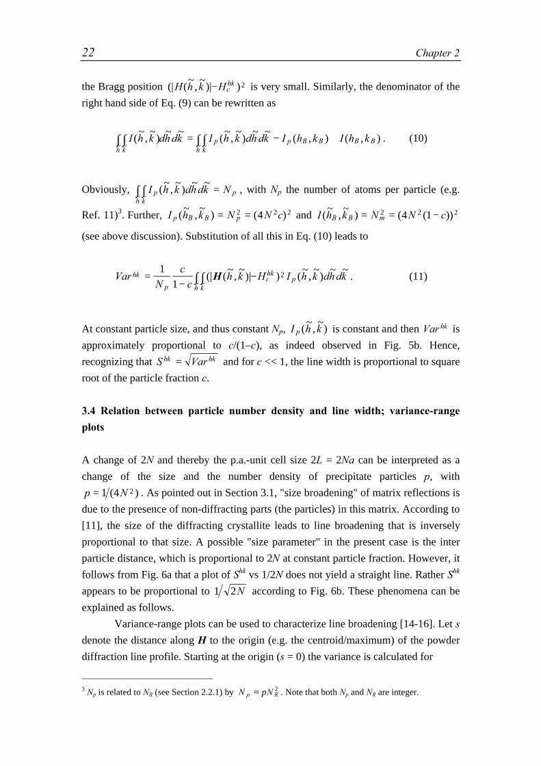
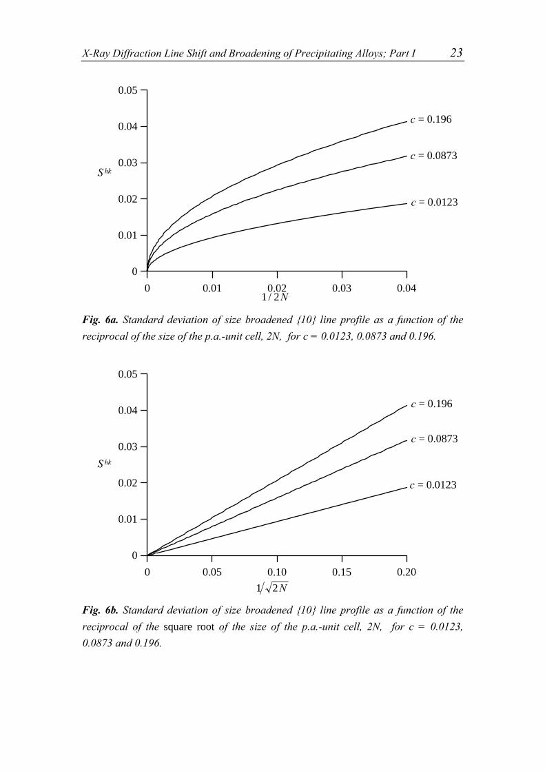
3.4 Relation between particle number density and line width; variance-range
plots
A change of 2N and thereby the p.a.-unit cell size 2L = 2Na can be interpreted as a
change of the size and the number density of precipitate particles p, with
p N= 1 4 2( ) . As pointed out in Section 3.1, "size broadening" of matrix reflections is
due to the presence of non-diffracting parts (the particles) in this matrix. According to
[11], the size of the diffracting crystallite leads to line broadening that is inversely
proportional to that size. A possible "size parameter" in the present case is the inter
particle distance, which is proportional to 2N at constant particle fraction. However, it
follows from Fig. 6a that a plot of Shk vs 1/2N does not yield a straight line. Rather Shk
appears to be proportional to 1 2N according to Fig. 6b. These phenomena can be
explained as follows.
Variance-range plots can be used to characterize line broadening [14-16]. Let s
denote the distance along H to the origin (e.g. the centroid/maximum) of the powder
diffraction line profile. Starting at the origin (s = 0) the variance is calculated for
3 Np is related to NR (see Section 2.2.1) by N Np R≈ π 2 . Note that both Np and NR are integer.
X-Ray Diffraction Line Shift and Broadening of Precipitating Alloys; Part I 23
0.05
0.04
0.03
0.02
0.01
0
0.040.030.020.010
c = 0.196
c = 0.0873
c = 0.0123
Fig. 6a. Standard deviation of size broadened {10} line profile as a function of the
reciprocal of the size of the p.a.-unit cell, 2N, for c = 0.0123, 0.0873 and 0.196.
0.05
0.04
0.03
0.02
0.01
0
0.200.150.100.050
c = 0.196
c = 0.0873
c = 0.0123
Fig. 6b. Standard deviation of size broadened {10} line profile as a function of the
reciprocal of the square root of the size of the p.a.-unit cell, 2N, for c = 0.0123,
0.0873 and 0.196.
1 2N
S hk
1 2/ N
S hk
24 Chapter 2
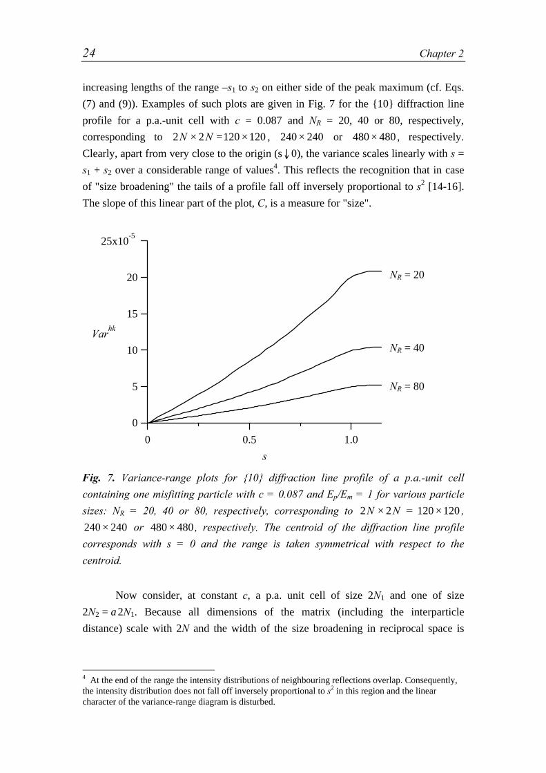
increasing lengths of the range –s1 to s2 on either side of the peak maximum (cf. Eqs.
(7) and (9)). Examples of such plots are given in Fig. 7 for the {10} diffraction line
profile for a p.a.-unit cell with c = 0.087 and NR = 20, 40 or 80, respectively,
corresponding to 2 2N N× =120 120× , 240 240× or 480 480× , respectively.
Clearly, apart from very close to the origin (s↓0), the variance scales linearly with s =
s1 + s2 over a considerable range of values4. This reflects the recognition that in case
of "size broadening" the tails of a profile fall off inversely proportional to s2 [14-16].
The slope of this linear part of the plot, C, is a measure for "size".
25x10-5
20
15
10
5
0
Varhk
1.00.50
s
Fig. 7. Variance-range plots for {10} diffraction line profile of a p.a.-unit cell
containing one misfitting particle with c = 0.087 and Ep/Em = 1 for various particle
sizes: NR = 20, 40 or 80, respectively, corresponding to 2 2N N× = 120 120× ,
240 240× or 480 480× , respectively. The centroid of the diffraction line profile
corresponds with s = 0 and the range is taken symmetrical with respect to the
centroid.
Now consider, at constant c, a p.a. unit cell of size 2N1 and one of size
2N2 = α2N1. Because all dimensions of the matrix (including the interparticle
distance) scale with 2N and the width of the size broadening in reciprocal space is
4 At the end of the range the intensity distributions of neighbouring reflections overlap. Consequently,the intensity distribution does not fall off inversely proportional to s2 in this region and the linearcharacter of the variance-range diagram is disturbed.
NR = 20
NR = 40
NR = 80
X-Ray Diffraction Line Shift and Broadening of Precipitating Alloys; Part I 25
proportional with 1/2N [11], one can write I s I sN N2 21 2( ) ( )α = with I the intensity
distribution along H. Thus
Var
s I s ds
I s ds
s I s ds
I s ds
s I s d s
I s d s
C s s C s s
Nhk
Ns
s
Ns
s
Ns
s
Ns
s
Ns
s
Ns
s2
22
2
22
2
22
2
1 2 1 2
2
2
1
2
2
1
2
1
1
2
1
1
2
1
1
2
1
1
2
1 1
= = ≅
≅ + = + =
−
−
−
−
−
−
∫
∫
∫
∫
∫
∫
( )
( )
( )
( )
( ) ( ) ( )
( ) ( )
( ) ( )
=1
1
2
2
α
αα
α α α
α α
αα α
α
α
α
α
α
αVar N
hk2 1
(12)
Here the approximation ( )I s d s I s d sNs
s
Ns
s
2 22
1
2
2
1
2
( ) ( ) ( )α α α αα
α
− −∫ ∫≅ has been applied, which
is justified when the tails of the intensity distribution have a negligible contribution to
the integrated intensity. It immediately follows from Eq. (12) that S Varhk hk ( )= is
inversely proportional to 2N , as observed (Fig. 6). Hence the line width is
proportional to (p)1/4.
The reason for Shk being related inversely proportional to 2N instead of 2N
is a direct consequence of the variance being defined to include all line intensities of
the {hk} reflection (see Eqs. 7 and 9), so that the length of the range, s1 + s2, is
independent of the width and the shape of the line profile. Had the lengths of the
ranges of I N2 1 and I N2 2
been scaled according to ( ) ( )s s s sN N1 2 2 1 2 21 2+ = +α , then
the calculation of the corresponding variances would have yielded the 1/2N-
dependence.
3.5 Effect of particle clustering
The simulations show that, although the {hk} diffraction line profiles of the matrix are
dependent on the state of particle clustering, for the case of pure "size broadening" the
centroid and the variance of these diffraction line profiles are practically unaffected by
clustering (see also discussion in Section 3.2 and footnote 4). Only for the utmost
clustered state when particles touch, the variance changes abruptly .
The effect of particle clustering can be clarified by comparing the Fourier
coefficients of the diffraction-line profiles for different states of clustering. As an
example, the real and imaginary parts of the Fourier coefficients, normalised by the
first Fourier coefficient and obtained using the tangent procedure (cf. Section 2.2.3),
have been plotted in Fig. 8 for Cf-values ranging from the unclustered state (Cf = 0) to

26 Chapter 2
the (utmost) clustered state where particles touch (with c = 0.087 it follows C fmax =
0.67, see Section 2.1) and 4 4N N× = 240 240× .
The imaginary parts of the Fourier coefficients of the {10} powder diffraction
line profile are zero independent of the state of particle clustering: the line profile
remains symmetric with respect to its origin as there is no shift of the centroid.
1
0.95
0.9
As(ξ)
12080400ξ
0
00.67
all Cf
real part
imaginary part
1–c/(1–c)
0.5 0.17
Fig. 8. Real and imaginary parts of Fourier coefficients As(ζ) of {10} powder
diffraction line profile, obtained using the tangent procedure, of a large p.a.-unit cell
containing 4 4N N× = 240 240× atoms and four non diffracting particles of radius
NR = 20 (c = 0.0873) located at (x,y) = (±Lp, ±Lp) = (±Nca, ±Nca), with
Nc = 60 (Cf = 0), Nc = 50 (Cf = 0.17), Nc = 30 (Cf = 0.50) and Nc = 20
(Cf = C fmax = 0.67).
1
0.995
0.99
As(ξ)
420ξ
0.67
0
C f = 0 67.
C f = 0 67.

X-Ray Diffraction Line Shift and Broadening of Precipitating Alloys; Part I 27
The real parts of the Fourier coefficients of the {10} powder diffraction line
profiles are clearly dependent on the state of clustering. It can be shown (see
Appendix D) that the "size Fourier coefficients" can be regarded as being the sum of a
constant level, As(ξ) = 1–c/(1–c) (As(ξ) ≈ 0.9 here), and the size Fourier coefficients of
the particles if they diffract and consist of matrix material. For Cf = 0 the large p.a.-
unit cell is in its unclustered state and As(ξ) is periodic with period 2N (2N = 120
here). If Cf > 0 the peak at ξ = 2N separates into two equal peaks of half heigth that
move either towards ξ = 0 or to ξ = 4N with a shift directly related to the state of
clustering.
According to a result of Fourier theory [17] the variance of the {hk} powder
diffraction line profile can be calculated from the curvature of the As(ξ)-curve at the
origin
VarA
d Ad
hk
s
s= −1
4 00
2
2
2π ξ( )( ) . (13)
Since the curvature of the As(ξ)-curve at the origin (Fig. 8) does not change
significantly with clustering, the variance remains constant for almost all values of Cf.
However, as soon as particles touch, i.e. Cf = C fmax , the curvature at the origin
changes, so that the variance changes. Physically this means that the clustered
particles cannot be considered as separate particles anymore.
4. "Size-strain separation"
If "size" and "(micro)strain" both contribute to line broadening, the problem arises
how to separate both contributions.
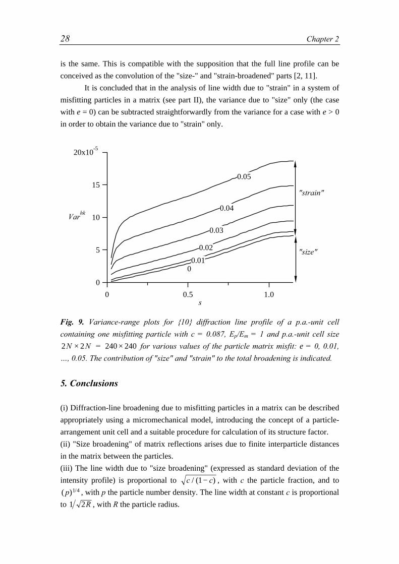
For the present case of misfitting particles in a matrix a series of variance-
range plots (calculated from the corresponding intensity distributions; cf. Section 3.4
and Fig. 7) is shown in Fig. 9 for a range of values for the misfit parameter ε. As
discussed in connection with Fig. 7 (where ε = 0: only "size" broadening") the slope of
the linear part of the curve with ε = 0 in Fig. 9 is representative of the "size
broadening": tails of the intensity distribution decay with 1/s2 [14-16]. It follows from
the results shown in Fig. 9 that (i) a linear part in the variance-range plots also occurs
for ε > 0, and (ii) that this slope is independent of ε. When one recognizes that "size"
dominates the tails of the intensity distribution at large values of s [14-16], these
results suggest that the variance of the "size broadening" occurring in all cases (ε > 0)
28 Chapter 2
is the same. This is compatible with the supposition that the full line profile can be
conceived as the convolution of the "size-" and "strain-broadened" parts [2, 11].
It is concluded that in the analysis of line width due to "strain" in a system of
misfitting particles in a matrix (see part II), the variance due to "size" only (the case
with ε = 0) can be subtracted straightforwardly from the variance for a case with ε > 0
in order to obtain the variance due to "strain" only.
20x10-5
15
10
5
0
Varhk
1.00.50s
"size"
"strain"
00.01
0.02
0.03
0.04
0.05
Fig. 9. Variance-range plots for {10} diffraction line profile of a p.a.-unit cell
containing one misfitting particle with c = 0.087, Ep/Em = 1 and p.a.-unit cell size
2 2N N× = 240 240× for various values of the particle matrix misfit: ε = 0, 0.01,
…, 0.05. The contribution of "size" and "strain" to the total broadening is indicated.
5. Conclusions
(i) Diffraction-line broadening due to misfitting particles in a matrix can be described
appropriately using a micromechanical model, introducing the concept of a particle-
arrangement unit cell and a suitable procedure for calculation of its structure factor.
(ii) "Size broadening" of matrix reflections arises due to finite interparticle distances
in the matrix between the particles.
(iii) The line width due to "size broadening" (expressed as standard deviation of the
intensity profile) is proportional to c c/ ( )1− , with c the particle fraction, and to
( ) /p 1 4 , with p the particle number density. The line width at constant c is proportional
to 1 2R , with R the particle radius.
X-Ray Diffraction Line Shift and Broadening of Precipitating Alloys; Part I 29
(iv) Clustering of particles does affect the powder diffraction line profiles, but it does
not affect the centroid and the variance due to "size" broadening as long as the
particles do not touch.
(v) For the case of misfitting particles in a matrix, the variances of the "size-" and
"strain-broadened" parts of the intensity distribution can be regarded as being additive
to a high accuracy. This implies that the variance of the "strain-broadened part" can be
obtained by subtraction of the variance observed in the case of pure "size broadening".
Acknowledgement
This work has been part of the research program of the Foundation for Fundamental
Research on Matter (Stichting FOM), The Netherlands.
Appendix A Interpolation of displacement field within an element
The displacement of an arbitrary point P in a quadrilateral element can be obtained by
bilinear interpolation between the displacements of its four nodes. First, the so-called
natural coordinates of P in a reference, square element are determined. Then, bilinear
interpolation of the displacements of each node using the natural coordinates yields
the displacement at P.
The natural coordinates (ξ,η) of P(x,y) are found from solving the following
matrix equation [10] for ξ and η
1 1 1 1 11 11 11 11 1
1 2 3 4
1 2 3 4
14141414
xy
x x x xy y y y
=
− −− ++ −+ +
( )( )( )( )( )( )( )( )
ξ ηξ ηξ ηξ η
. (A. 1)
with (xi,yi) the coordinates of the four nodes of the quadrilateral element. Working out
the matrix product of Eq. (A. 1), two non linear coupled equations are obtained
44
1 2 3 4
1 2 3 4
xy
a a a ab b b b
=
+ + ++ + +
ξ η ηξξ η ηξ
(A. 2)
with ai and bi given by

30 Chapter 2
1 1 1 11 1 1 11 1 1 11 1 1 1
1 1
2 2
3 3
4 4
1 1
2 2
3 3
4 4
− −− −
− −
=
x yx yx yx y
a ba ba ba b
. (A. 3)
After elimination of the term ξη in Eq. (A. 2), ξ can be expressed in η as
ξ η= +c c1 2 (A. 4)
with
cb x a y a b a b
a b a bc
a b a ba b a b
14 4 1 4 4 1
2 4 4 22
3 4 4 3
2 4 4 2
4=
− − −−
= −−−
( ) ( ); (A. 5)
Subsequently, the relation between ξ and η is used in Eq. (A. 2) to obtain a quadratic
equation in η of the type e e e12
2 3 0η η+ + = , with e1, e2 and e3 as known constants,
which can be readily solved. Two solutions η1 and η2 are obtained that correspond
with ξ1 and ξ2, respectively, using Eq. (A. 4). However, since ξ and η are defined such
that –1 < ξ, η < 1 only one set of coordinates (ξ,η) is found.
The displacements (u, v) at P are finally calculated by means of the same
interpolation as in Eq. (A.1) [10]
1 1 1 1 11 11 11 11 1
1 2 3 4
1 2 3 4
14141414
uv
u u u uv v v v
=
− −− ++ −+ +
( )( )( )( )( )( )( )( )
ξ ηξ ηξ ηξ η
(A. 6)
with ui, vi the displacements of the four nodes of the quadrilateral element.
Appendix BCalculation of the structure factor using the Fast Fourier Transform
algorithm
The calculation of the structure factor of the p.a.-unit cell can be carried out
straightforwardly using Eqs. (3) and (4) (cf. Section 2.2.2). To improve the speed of
this calculation, these formulae are rewritten in a form that enables the use of a Fast
Fourier Transform algorithm. The discussion in this appendix is limited to a one-

X-Ray Diffraction Line Shift and Broadening of Precipitating Alloys; Part I 31
dimensional case, although the method can be adapted easily and straightforwardly to
two and three dimensional cases.
B. 1. One-dimensional particle arrangement unit cell
The one-dimensional analogon of the two-dimensional p.a.-unit cell is displayed in
Fig. B1. It consists of a row of 2N atoms with a one-dimensional (misfitting)
"particle" at the center (origin of x-axis). This one-dimensional p.a. unit cell is
described in analogy with the two-dimensional p.a.-unit cell by a p.a.-unit cell vector~a , which is equal to ~a a= 2N with a the matrix unit-cell vector and a = a the atomic
distance. The structure factor of this p.a.-unit cell, with rn the position of atom (n)
with respect to the origin of the p.a.-unit cell and f n the scattering factor of atom (n),
is given by (cf. Eq. (3))
F h f eni
n
N(~
) = ⋅
=
−∑ 2
0
2 1π H rn . (B. 1)
The one-dimensional diffraction vector H b= ~~h is expressed in terms of the real-
valued variable ~h and the reciprocal lattice vector ~b , ( ~ ~
a b⋅ = 1). The "~" symbol is
used to mark all variables directly related to the p.a.-unit cell vector ~a .
Each vector rn is expressed by means of a fractional coordinate ~X n , i.e.
r an nX= ~ ~ . In the deformed state, the fractional coordinates are written as (cf. Eq. (4))
~ ( )X
n N a uNa Un
n=+ − +
+
12
2 2(B. 2)
with un the displacement of atom n from its undeformed position ( )n N a+ −12 .
Combining Eqs. (B. 1) and (B. 2), the one dimensional p.a.-unit cell structure factor is
given by
F h f enih
n N a u
Na Un
N n
(~
)~ ( )
=+ − +
+=
−∑ 2
2 20
2 1 12π
(B. 3)
As explained in Section 2.2.2, F h(~
) for an infinitely large crystal needs only be
calculated at integer positions within the range 2(hB–1/2)N < ~h < 2(hB+1/2)N, where
hB denotes the value of h at a Bragg position according to the one-dimensional matrix
unit cell description.

32 Chapter 2
x
Fig. B.1. Schematic presentation of the redefinition of the displacement field of
(particle and) matrix atoms in a one-dimensional p.a.-unit cell of 2N = 20 and NR =
2; only the right half of the p.a.-unit cell is shown. In (a) the positions of the atoms in
the deformed state are shown. In (b) the reference lattice positions are shown. The
displacement of a matrix atom from its strain free, reference lattice, position is
redefined as the displacement from the nearest reference lattice position. This is
indicated in (a) and (b) by the dotted lines that connect the displaced atoms with the
nearest reference lattice position. These atoms are denoted "regular" atoms. If no
matrix atom is close enough to a specific reference lattice point then that reference
lattice point is conceived as a vacancy, indicated by the " "-symbol in (b). If more
than one atom is close to the same reference lattice point the one closest to this lattice
point is selected. The remaining one is considered an "interstitial" type of atom (see
(c)). The calculation of the structure factor is performed in two parts: one part uses
the FFT-method of Eq. (B. 10) which includes all regular atoms and the local
vacancies and the other part uses the fundamental description (Eq. (B. 9)) for the
"interstitial" type of atoms.
The total number of calculations necessary to calculate the intensity
distribution of an {hB} reflection is dependent on the square of the number of atoms
within the p.a.-unit cell: for every single line intensity, 2N summations have to be
carried out in Eq. (B. 3) and every {hB} reflection consists of the same number of line
intensities.
(a)
(b)
(c)
particle matrix
"regular" atoms
"interstitial" atomsn=N 2N–1 . .

X-Ray Diffraction Line Shift and Broadening of Precipitating Alloys; Part I 33
B. 2. Calculation of the structure factor using the discrete Fourier transform
The discrete Fourier transform P(t) of an arbitrary discrete function p(m) of period M
is given by [17]
P tM
p m e itm
Mm
M( ) ( )=
=
−∑
1 2
0
1 π (B. 4)
where both the real space variable, m, and the Fourier space variable, t, are integers,
here. Comparing this equation with Eq. (B. 3) (M = 2N), we see that Eq. (B. 3) cannot
be considered a discrete Fourier transform due to the contribution of the displacement
field in the numerator and denominator of the exponent of Eq. (B. 3). However, Eq.
(B. 3) can be rewritten such that an equation similar to Eq. (B. 4) is obtained.
Firstly, a new lattice constant is defined for the deformed p.a.-unit cell. In thedeformed state, the length of the p.a.-unit cell vector equals ~a = +2 2Na U . A new(average) lattice constant ad is defined such that ~a = 2Nad and a a U Nd = + . Then,
the displacement und of an atom from its undeformed position given by the new lattice
constant can be expressed as
u u n NUNn
dn= − + −( )1
2 . (B. 5)
The structure factor according to. Eq. (B. 3) can now be rewritten as
F h f enih
n N u a
Nn
N nd
d
(~
)~ ( )
=+ − +
=
−∑ 2
20
2 1 12π . (B. 6)
Secondly, the diffraction vector is expressed in terms of the deviation from
the Bragg position (in terms of the p.a.-unit cell description: at the Bragg position~h NhB B= 2 ; see at the end of Section 2.2.2): H b )b= =~~
(~ ~
h Nh + hB2 ∆ , or~ ~h Nh hB= +2 ∆ . Note that since
~h and 2NhB
~ are integers, ∆~
h is integer too.
Now Eq. (B. 6) can be split up into a displacement-dependent part and a
displacement-independent part:

34 Chapter 2
F h f e e enih u a i
h u aN
ih nN
n
NB n
dd
nd
d
(~
)
~ ~
==
−∑ 2 2
22
2
0
2 1π π π
∆ ∆
(B. 7)
where the term (n+1/2-N) has been reduced to n as this leaves the value of
F h F h(~
) (~
)* unaffected. Although the third exponential on the right hand side of Eq.
(B. 7) is similar to the exponential given in Eq. (B. 4), Eq. (B. 7) is not a discrete
Fourier transform since the second exponential on the right hand side of Eq. (B. 7)
depends on ∆~h .
Next, the second exponential on the right hand side of Eq. (B. 7) is written as a
Taylor series expansion leading to
( ) ( )[ ]F hi h N
tf u a e e
t
tn n
dd
t ih u a ih n
N
n
NB n
dd(
~)
~
!
~
=
=
∞
=
−∑ ∑
2 2
0
2 22
0
2 1ππ π∆ ∆
(B. 8)
The term within braces represents the discrete Fourier transform of the function in
square brackets (cf. Eq. (B. 4)). The structure factor is computed by a finite sum of
such Fourier transforms. For the 2D case considered in this work Eq. (B. 8) has been
summed up to t = 8, leading to a relative error in the value of the variance smaller than
10-4 %.
The number of terms of the Taylor series expansion necessary to calculate
accurately the structure factor is limited only if the displacements are small compared
to ad. However, in the immediate neighbourhood of misfitting particles, displacements
of the order of several atomic distances can occur. This may seriously destroy the
convergence of the series, especially for large deviations from the Bragg position. This
can be remedied in the following way.
For the calculation of the structure factor the locations of all atoms in the
deformed state are considered and therefore it is not important from which reference
lattice points the atoms were displaced (cf. Fig. B1). Thus, the displacement of an
atom over several atomic distances can also be conceived as a displacement from a
different reference lattice point over a distance smaller than the atomic distance. In
this way the displacement of all atoms is redefined as the displacement from the
nearest reference lattice point. Thus, all atomic displacements remain smaller than half
of the atomic distance and only a few terms of the Taylor series expansion (B. 8) need
to be taken into account. Following this procedure, only one atom is allocated to most
reference lattice points; these atoms are denoted "regular" atoms from now on.
However, two special cases need to be considered: (i) two or more atoms are close to

X-Ray Diffraction Line Shift and Broadening of Precipitating Alloys; Part I 35
the same reference lattice point and (ii) no atom is close enough to a specific reference
lattice point (see Fig. B1).
In the first case, only one atom can be assigned to the reference lattice point.
The contributions to the structure factor of the remaining, "interstitial" type of atoms
(see Fig. B1) cannot be calculated by the discrete Fourier transform method but
requires application of the fundamental equation, similar to Eq. (B. 3):
F h f e i
n
N
int n n
int
int
(~
) = ⋅
=∑ 2
1
π H r (B. 9)
with Nint the total number of "interstitials".
In the second case, no atom is close enough to a specific reference lattice point
and, consequently, there is no contribution of this reference lattice point to the
structure factor. Hence it can be treated as a vacancy. In the calculation of the structure
factor this is handled by setting the atomic scattering factor fn for this reference lattice
point equal to zero. (Since the total number of atoms remains unchanged it is clear
that the number of "vacancies" equals the number of "interstitial" type atoms).
Finally, the structure factor of the p.a.-unit cell in the deformed state equals the
sum of the contribution of all "regular" atoms and all "interstitial" atoms, i.e.
( )F h
i h N
tf u a e e f e
t
tn n
dd
tih u a i
h n
Nn
N
ni
NB n
dd(
~)
~
!
~
=
+
=
∞ ∧ ∧
=
−⋅
=∑ ∑ ∑
∧2 2
0
2 22
0
2 12
1
ππ π π
∆ ∆H rn
int
int
n(B.10)
where f n
∧ indicates the atomic scattering factor ( f fn n
∧= for an atom and f n
∧= 0 for
a vacancy) and u nd
∧ indicates the redefined displacement field that assigns to each
reference lattice points a displacement smaller than half of the atomic distance.
The calculation of the structure factor using Eq. (B. 10) is much faster than
that using Eq. (B. 3): the calculation on the basis of Eq. (B. 3) increases quadraticly
with the number of atoms (cf. Section B.1), whereas the calculation on the basis of Eq.
(B. 10) increases approximately linearly with the number of atoms. The total number
of calculations on the basis of Eq. (B. 10) can be assessed as follows. The contribution
of the majority of atoms to the structure factor is calculated using a Fast Fourier
Transform algorithm. The calculation of the discrete Fourier transform of 2N
datapoints is proportional to 2N log(2N) [17]. If the number of terms used in the
Taylor series expansion equals tmax, the total number of calculations for the "regular"
atoms thus scale as 2Ntmax log(2N). The number of calculations for the "interstitial"

36 Chapter 2
type atoms scale as Nint2N (see discussion below Eq. (B. 3)). Thus, the total number of
calculations for the structure factor on the basis of Eq. (B. 10) scale as
2N(tmaxlog(2N)+Nint) with Nint << 2N, which shows that for large values of 2N this
number increases approximately linearly with 2N.
B. 3. Simplified calculation of the structure factor
If ∆~h is small ( ∆~
h N<< ) the second exponential on the right hand side of Eq. (B. 7)
can be neglected, which is equivalent to a maximum value of t in Eq. (B. 7) of t = 0,
and a simplified, approximate, again discrete Fourier transform expression for the
structure factor results
F h f e eapprox nih u a i
h n
N
n
NB n
dd(
~)
~
==
−∑ 2 2
2
0
2 1π π
∆
(B. 11)
The simplification is equivalent to replacing H r⋅ in Eq. (B. 1) by H rB ⋅ . In
standard treatments of X-ray diffraction (e.g. Warren [11]) this same approximation is
carried out in the calculation of line profiles. The real-valued variable h3 in reciprocal
space is replaced by the order of reflection l of a {00l}-type reflection and only the
component of displacement of unit cell m along the h3-axis, Zm, is considered.
Appendix CInfluence of the rotation procedure on the centroid and variance of the
{hk} powder diffraction line profile
A powder diffraction line profile can be obtained from the intensity distribution in
reciprocal space of a single powder particle using the rotation procedure (cf. Section
2.3). This procedure causes an intensity distribution of a single powder particle that is
symmetrical in reciprocal space to become slightly asymmetrical after projection onto
the diffraction vector. The asymmetry leads to an additional shift of the centroid (cf.
Fig. 5a) which is proportional to the variance of the powder diffraction line profile as
is proven here.
The position of an {~~
}h k line intensity in reciprocal space, H(h k )~, ~ , is
described as the sum of the vector indicating the Bragg position of the reflection
considered, HB, and a vector describing the deviation from the Bragg position,
∆H(h ,k )~ ~

X-Ray Diffraction Line Shift and Broadening of Precipitating Alloys; Part I 37
H H H(h ,k) (h ,k)B~ ~ ~ ~= + ∆ (C. 1)
The distance of the {~~
}h k line intensity to the origin of reciprocal space, |~ ~
|H(h ,k) ,
follows from Eq. (C. 1) as
H HH H
H
H
H(h ,k)
(h ,k ) (h ,k)B
B
B B
~ ~~ ~ ~ ~
= +⋅
+1 2 2
2
2
∆ ∆(C. 2)
Since in Eq. (C. 2) the second and third term inside the square root are small
compared to the first one, the square root can be approximated by a Taylor series.
Using the first term of the Taylor series expansion only, Eq. (C. 2) can be simplified
to
H H HH
H
H
H(h ,k) (h ,k)
(h ,k )B
B
B B
~ ~ ~ ~~ ~
≅ + ⋅ +∆∆1
2
2
(C. 3)
Using this equation to calculate the centroid position according to Eq. (6) (cf. Section
2.3) in case of the rotation procedure yields
HI h ,k h ,k
I h ,k
I h ,k h ,k
I h ,kc rothk
BB
B
B,
(~ ~
) (~ ~
)
(~ ~
)
(~ ~
) (~ ~
)
(~ ~
)= + +
⋅∑∑∑∑
∑∑∑∑
HH
H H
H
H 21 12
∆ ∆
(C. 4)
with the subscript "rot" denoting the rotation procedure. The second term on the right
hand side of Eq. (C. 4) expresses the projection of ∆H(h k )~
,~
perpendicularly onto the
diffraction vector HB as is the case applying the tangent procedure. Thus, the sum of
the first and the second term corresponds exactly to the centroid that would have been
obtained if the tangent procedure had been used. Consequently, the third term
expresses the difference between the tangent and the rotation procedure. This term is
proportional to the square of the distance of the matrix Bragg reflection H B to the
{~~
}h k line intensity, ∆H 2(h ,k )~ ~
, and can be interpreted in terms of the variance of this
line profile.
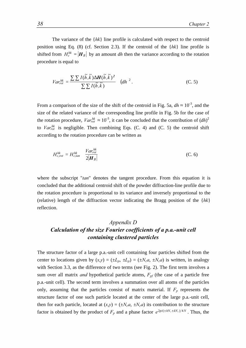
38 Chapter 2
The variance of the {hk} line profile is calculated with respect to the centroid
position using Eq. (8) (cf. Section 2.3). If the centroid of the {hk} line profile is
shifted from Hchk
B= H by an amount δh then the variance according to the rotation
procedure is equal to
( )VarI h ,k h ,k
I h ,khrot
hk = +∑∑
∑∑(~ ~
) (~ ~
)
(~ ~
)
∆H 2
δ 2 . (C. 5)
From a comparison of the size of the shift of the centroid in Fig. 5a, δh ≈ 10-3, and the
size of the related variance of the corresponding line profile in Fig. 5b for the case of
the rotation procedure, Varrothk ≈ 10-3, it can be concluded that the contribution of (δh)2
to Varrothk is negligible. Then combining Eqs. (C. 4) and (C. 5) the centroid shift
according to the rotation procedure can be written as
H HVar
c rothk hk rot
hk
B, = +c,tan
2 H(C. 6)
where the subscript "tan" denotes the tangent procedure. From this equation it is
concluded that the additional centroid shift of the powder diffraction-line profile due to
the rotation procedure is proportional to its variance and inversely proportional to the
(relative) length of the diffraction vector indicating the Bragg position of the {hk}
reflection.
Appendix DCalculation of the size Fourier coefficients of a p.a.-unit cell
containing clustered particles
The structure factor of a large p.a.-unit cell containing four particles shifted from the
center to locations given by (x,y) = (±Lp, ±Lp) = (±Nca, ±Nca) is written, in analogy
with Section 3.3, as the difference of two terms (see Fig. 2). The first term involves a
sum over all matrix and hypothetical particle atoms, Fpf (the case of a particle free
p.a.-unit cell). The second term involves a summation over all atoms of the particles
only, assuming that the particles consist of matrix material. If Fp represents the
structure factor of one such particle located at the center of the large p.a.-unit cell,
then for each particle, located at (x,y) = (±Nca, ±Nca) its contribution to the structure
factor is obtained by the product of Fp and a phase factor e i hN kN Nc c2 4π ( )± ± . Thus, the

X-Ray Diffraction Line Shift and Broadening of Precipitating Alloys; Part I 39
structure factor of the p.a.-unit cell containing all four particles, F h k(~
,~
) , can be
expressed as (cf. Eq. (8))
F h k F Fpf p(~
,~
) = − α (D. 1)
with
απ π
=
4
24
24
cos~
cos~
h NN
kNN
c c(D. 2)
The intensity distribution in reciprocal space of a single crystal composed of an
infinite number of p.a.-unit cells equals, according to Section 2.2.2,
I h k F h k F h k(~
,~
) (~
,~
) (~
,~
)*= at integer values of ~h and
~k . Writing
F h k F h k I h kp p p(~
,~
) (~
,~
) (~
,~
)* = , it follows that (cf. Eq. (10))
I h k I h k I h k I h kp p B B B B(~
,~
) (~
,~
) ( , ) ( , )= − +α 2 . (D. 3)
The intensity distribution has two contributions: (i) at the Bragg position
I h k N cB B(~
,~
) ( ( ))= −16 12 2 (see below Eq. (10)) and (ii) at non-Bragg positions the
intensity distribution in reciprocal space equals the intensity distribution that would
have been obtained if only particles made of matrix materials had diffracted,
I h k I h kp(~
,~
) (~
,~
)= α 2 , where α2 can be expressed as
[]
α π π
π π
2 4 1 4 4 4 4
4 4 4 4
= + + +
+ + −
cos(~
) cos(~
)
cos( (~ ~
) ) cos( (~ ~
) )
h N N kN N
h k N N h k N N
c c
c c
(D. 4)
Now, on the basis of Eqs. (D.3) and (D. 4) the (2D) size Fourier coefficients of
I h k(~
,~
) , normalised by the first Fourier coefficient, As ( , )ξ ζ , consist of the sum of
the Fourier coefficients of two contributions. The normalised Fourier coefficients of
the first contribution can be expressed as A c csi( ) ( , ) / ( )ξ ζ = − −1 1 , i.e. a constant
level independent of the degree of clustering.
The Fourier coefficients of the second contribution, Asii( ) ( , )ξ ζ , represent the
Fourier coefficients of the hypothetically diffracting particles made of matrix material;
they can be calculated in the following way (see Eq. (D. 4)). If the Fourier coefficients

40 Chapter 2
of I h kp (~
,~
) equal Asp ( , )ξ ζ , with ξ and ζ as the (harmonic) numbers, then according
to Fourier theory [17], the Fourier coefficients of I h k h Np (~
,~
) cos(~
)4 4πω equal
[ ( , ) ( , )] /A N A Nsp
c sp
cξ ζ ξ ζ+ + − 2 , i.e. the Fourier coefficients consist of half the
sum of two replicas of Asp ( , )ξ ζ shifted by an amount of ±Nc along
~b1 . In the same
way, the contribution of other terms of α2 to Asii( ) can be calculated giving rise to an
unshifted replica of Asp ( , )ξ ζ located at the origin of reciprocal space and shifted
replicas displaced by amounts (0, ±Nc) and (±Nc, ±Nc), respectively.
Thus, the size Fourier coefficients of the intensity distribution of a p.a.-unit cell
containing four non-diffracting particles clustered along x = ±y can be conceived as the
sum of a constant level and unshifted replica of the size Fourier coefficients of
hypothetically diffracting particles made of matrix material and four pairs of shifted
replicas.
References
[1] G.E. Dieter, Mechanical Metallurgy, McGraw-Hill, Singapore, 1987.
[2] R. Delhez, Th.H. de Keijser and E.J. Mittemeijer, Fresenius Z. anal. Chem. 312 (1982) 1 -
16.
[3] J.G.M. van Berkum, A.C. Vermeulen, R. Delhez, Th.H. de Keijser and E.J. Mittemeijer,
J. Appl. Cryst. 27 (1994) 345 - 357.
[4] J.G.M. van Berkum, R. Delhez, Th.H. de Keijser and E.J. Mittemeijer, Acta Cryst. A52
(1996) 730 - 747.
[5] P. van Mourik, Th.H. de Keijser, N.M. van der Pers and E.J. Mittemeijer, Scripta Metall.
22 (1988) 1547 - 1551.
[6] S. Iida, B.C. Larson, J.Z. Tischler, J. Mater. Res. 3(2), (1988), 267 - 273.
[7] J.G.M. van Berkum, R. Delhez, Th.H. de Keijser, E.J. Mittemeijer, P. van Mourik, Scripta
Metall. Mater. 25 (1991), 2255 - 2258.
[8] C.R. Houska, Acta Cryst. A49 (1993), 771 - 781.
[9] J.D. Eshelby, Solid State Phys. 3 (1956), 79 - 144.
[10] O.C. Zienkiewics, The Finite Element Method in Engineering Science, McGraw-Hill,
London, 1971.
[11] B.E. Warren, X-ray Diffraction, Reading, Massachusetts: Addison-Wesley, 1969.
[12] Von Laue, Z. Kristallogr. 64 (1926) 115 - 142.
[13] M.A. Krivoglaz, X-ray and Neutron Diffraction in Nonideal Crystals, Springer, Berlin,
1996.
[14] A.J.C. Wilson, Proc. Phys. Soc. 80, 286 - 294, 1962.
[15] A.J.C. Wilson, Proc. Phys. Soc. 81, 41 - 46, 1963.
[16] J.I. Langford, A.J.C. Wilson, In: Crystallography and Crystal Perfection, ed. G.N.
Ramachandran, Academic Press, 207 - 222, London, 1963.
[17] R.N. Bracewell, The Fourier Transform and its Applications, McGraw-Hill, Tokyo,
1978.

Chapter 3
X-Ray Diffraction Line Shift and Broadening ofPrecipitating Alloys
Part II: Study of "Strain" Broadening Effects
T.C. Bor1,2, R. Delhez1, E.J. Mittemeijer1,3 and E. Van der Giessen2
1Laboratory of Materials Science, Delft University of Technology,
Rotterdamseweg 137, 2628 AL Delft, The Netherlands2Koiter Institute Delft, Delft University of Technology,
Mekelweg 2, 2628 CD Delft, The Netherlands3Max Planck Institute for Metals Research,
Seestraße 92, 70174 Stuttgart, Germany
Abstract
The effects of misfitting precipitates in a polycrystalline matrix on the shift and broadening
of diffraction-line profiles are investigated applying a novel approach to the simulation and
interpretation of diffraction line profiles. The strain fields are calculated in two ways by
using (i) a numerical analysis for a unit cell containing one or a few precipitates and (ii) an
analytical, Eshelby-type approximation. The diffraction-line profiles are computed as a
function of the precipitate-matrix misfit, the elastic moduli of precipitates and matrix, the
volume fraction of precipitates and the degree of precipitate clustering. The relations
between the characteristics of the strain fields and the shifts and broadenings of the
diffraction-line profiles are established. Against this background, the approximations
traditionally applied in X-ray diffraction analysis are critically analyzed.
1. Introduction
X-ray diffraction measurements of materials containing a dispersion of particles
exhibit shift and broadening of diffraction-line profiles, as compared to the particle-
free situation [1, 2]. The line shift can be caused by a change of the overall lattice
parameter, caused for instance by a change of composition upon precipitation, or, less
obviously, by the development of a hydrostatic (macroscopic) stress component [3].
The line broadening can be caused by "size" and "microstrain" effects.
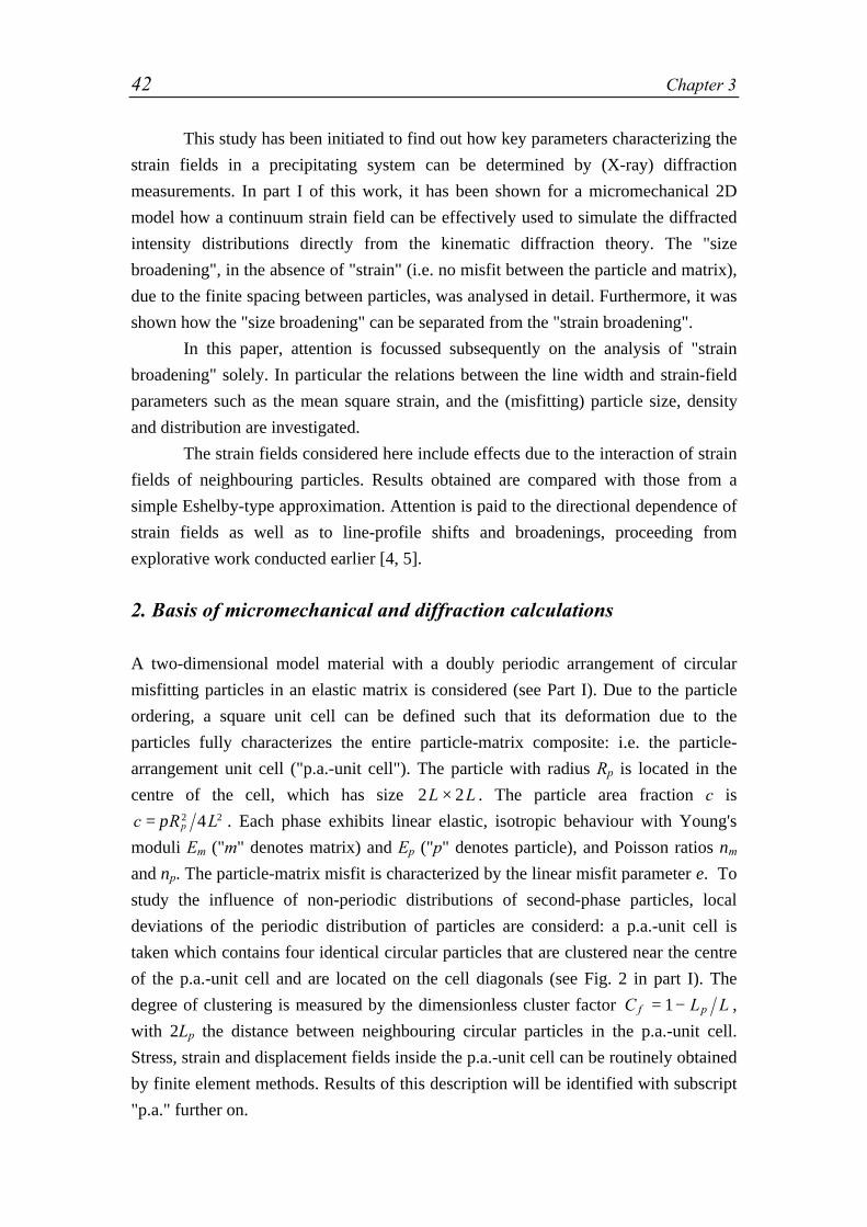
42 Chapter 3
This study has been initiated to find out how key parameters characterizing the
strain fields in a precipitating system can be determined by (X-ray) diffraction
measurements. In part I of this work, it has been shown for a micromechanical 2D
model how a continuum strain field can be effectively used to simulate the diffracted
intensity distributions directly from the kinematic diffraction theory. The "size
broadening", in the absence of "strain" (i.e. no misfit between the particle and matrix),
due to the finite spacing between particles, was analysed in detail. Furthermore, it was
shown how the "size broadening" can be separated from the "strain broadening".
In this paper, attention is focussed subsequently on the analysis of "strain
broadening" solely. In particular the relations between the line width and strain-field
parameters such as the mean square strain, and the (misfitting) particle size, density
and distribution are investigated.
The strain fields considered here include effects due to the interaction of strain
fields of neighbouring particles. Results obtained are compared with those from a
simple Eshelby-type approximation. Attention is paid to the directional dependence of
strain fields as well as to line-profile shifts and broadenings, proceeding from
explorative work conducted earlier [4, 5].
2. Basis of micromechanical and diffraction calculations
A two-dimensional model material with a doubly periodic arrangement of circular
misfitting particles in an elastic matrix is considered (see Part I). Due to the particle
ordering, a square unit cell can be defined such that its deformation due to the
particles fully characterizes the entire particle-matrix composite: i.e. the particle-
arrangement unit cell ("p.a.-unit cell"). The particle with radius Rp is located in the
centre of the cell, which has size 2 2L L× . The particle area fraction c is
c R Lp= π 2 24 . Each phase exhibits linear elastic, isotropic behaviour with Young's
moduli Em ("m" denotes matrix) and Ep ("p" denotes particle), and Poisson ratios νm
and νp. The particle-matrix misfit is characterized by the linear misfit parameter ε. To
study the influence of non-periodic distributions of second-phase particles, local
deviations of the periodic distribution of particles are considerd: a p.a.-unit cell is
taken which contains four identical circular particles that are clustered near the centre
of the p.a.-unit cell and are located on the cell diagonals (see Fig. 2 in part I). The
degree of clustering is measured by the dimensionless cluster factor C L Lf p= −1 ,
with 2Lp the distance between neighbouring circular particles in the p.a.-unit cell.
Stress, strain and displacement fields inside the p.a.-unit cell can be routinely obtained
by finite element methods. Results of this description will be identified with subscript
"p.a." further on.

X-Ray Diffraction Line Shift and Broadening of Precipitating Alloys; Part II 43
In the case that the p.a.-unit cell contains a single particle, an approximate
solution can be obtained, following a suggestion by Eshelby [6]. First the 2 2L L×matrix is replaced by a circular matrix with an effective radius of R Lm
eff = 2 π , so
that the particle fraction is the same. Then, the classical Eshelby solution is used for a
misfitting particle in an infinite matrix, corrected so that the traction at the matrix
outer radius Rmeff vanishes. The solution is given in Appendix A. Due to the finite
radius of the matrix, some elastic interaction between particles is accounted for
effectively, but, obviously, the directionality of the strain field due to the specific
distribution of the precipitates is absent in this approximate description. Results of this
approximate description will be identified with subscript "Esh" further on.
The calculation of a powder diffraction line profile is briefly summarized here;
see part I for a full discussion. The p.a.-unit cell is filled with a square grid of atoms at
an atomic distance a in the undeformed state. The displacement field, induced by the
misfitting particle in the matrix, is sampled at the locations of the atoms. The kinematic
diffraction theory is then used to calculate the intensity distribution in reciprocal space
from the position of the displaced atoms in the p.a.-unit cell. Powder diffraction line
profiles are obtained by projecting the line intensities in reciprocal space onto the
diffraction vector by either an exact, rotation procedure or by an approximative, yet
commonly applied, procedure, called the tangent procedure.
The "size" contribution to the intensity distribution is eliminated by means of the
method discussed in part I.
3. Characterization of strain fields and line profiles
The {hk}-powder diffraction-line profile contains information on strain components
ehk in the ⟨ ⟩hk -directions only [1]. Therefore, the matrix-strain field is characterized
in ⟨ ⟩hk -directions by the probability distribution of matrix strains, P(ehk), the average
local strain ⟨ ⟩ehk and the root mean squared local strain ⟨ ⟩ehk2 . The last measure is
defined here with respect to ⟨ ⟩ehk as
( )⟨ ⟩ =
− ⟨ ⟩∫∫
∫∫e
e e dxdy
dxdyhk
hk hkA
A
m
m
2
2
, (1)
where Am is the matrix part of the p.a.-unit cell and where x and y denote Cartesian
coordinates with the origin at the centre of the p.a.-unit cell, (cf. Fig. 1 in part I). In the

44 Chapter 3
finite element solution the contribution of a finite element is obtained from the
average of the values at the four integration points of that element [7].
Due to the symmetry of the p.a.-unit cell it can be proven that ⟨ ⟩ehk is
independent of the ⟨ ⟩hk -directions and hence it represents the hydrostatic strain (see
Appendix B). Therefore the subscript "hk" will be omitted for the average strain ⟨ ⟩e
in remainder of this paper.
Obviously, the Eshelby-type approximate solution is inherently independent of
the ⟨ ⟩hk -directions because of the circular symmetry.
The {hk} powder diffraction-line profile consists of a series of {~~
}h k line
intensities, I h k(~
,~
) . It is characterized by its centroid Hchk , as a measure of profile
position, and its standard deviation S hk , as a measure of profile width. Here,
Hh k I h k
I h kchk kh
kh
=∑∑
∑∑
| (~
,~
)| (~
,~
)
(~
,~
)
~~
~~
H, (2)
with | (~
,~
)|H h k the distance from the origin of reciprocal space to a specific {~~
}h k line
intensity obtained by projection onto the diffraction vector by either the tangent
procedure or the rotation procedure (cf. part I), and
( )S Varh k H I h k
I h khk hk
chk
kh
kh
2
2
= =−∑∑
∑∑
(| (~
,~
)| ) (~
,~
)
(~
,~
)
~~
~~
H(3)
with Varhk as the variance of the profile considered (defined with respect to Hchk ).
Diffraction estimates for ⟨ ⟩e and ⟨ ⟩ehk2 can be obtained from Hc
hk and Varhk
as follows. The centroid of a (strain broadened) line-profile, Hchk , is indicative of the
average lattice spacing in the diffracting material. Thus, with dhk and dhk0 as the
(average) lattice spacings for the strained and strain-free material, and Hchk and Hc
hk,0
as the corresponding centroids in reciprocal space, it follows
⟨ ⟩ =−
=−
ed d
d
H H
Hhk XRDhk hk
hk
chk
chk
chk
0
00
0
1 1
1,
,. (4)
where the subscript "XRD" is used to indicate that the concerned measure for strain is
derived from the diffraction-line profiles. A prerequisite for the above is that the
relative displacements of adjacent unit cells are small compared to the unit cell

X-Ray Diffraction Line Shift and Broadening of Precipitating Alloys; Part II 45
dimensions [8-10]. This will reasonably be the case if the linear misfit parameter is not
chosen larger than, say, ε = 5 %. Even in the case of incompressible misfitting particles
(Ep/Em → ∞ ), it can be shown with the aid of Appendix B, that the strains in the matrix
at the particle/matrix interface (r = Rp) are of the same order of magnitude as ε.
The variance of the strain broadened profile, Var hkε , is obtained by subtraction
of the variance of the merely size broadened profile, Var Shk hkε ε= =0
2( ) . According to [8 -
10] , this variance is a measure of the root mean squared strain,
⟨ ⟩ =eH
Shk XRDchk
hk2
0
1
,ε . (5)
4. Analysis of misfit-strain fields
4.1. Role of particle fraction; orientation dependence of strain parameters
The average local matrix strain ⟨ ⟩e has been calculated as a function of the particle
fraction c for values of E Ep m equal to 0.1, 1 and 10, in the unclustered state.
Throughout this work the Poisson ratios of particle and matrix have been taken equal:
νm = νp = 0.3. The results for ⟨ ⟩e are shown in Fig. 1 both for the numerical p.a.-unit
cell analysis ("p.a.") and the analytical Eshelby-type analysis ("Esh"). The average
local matrix strains ⟨ ⟩e Esh and ⟨ ⟩e p a. . obviously increase with the particle fraction c
(exactly linearly for E Ep m = 1 in the "Esh"-approximation; see Appendix B), with
the increase being larger for larger ratio E Ep m . This reflects the fact that a larger
part of the misfit has to be accommodated by the matrix if the particle becomes
relatively more rigid. The differences between the "p.a." and the "Esh" results are very
small up to large particle fractions and for a wide range of E Ep m . In Fig. 1,
differences become visible only for particle fractions above c = 0.25 at E Ep m = 10.
So, the average matrix strain obtained from the direction-independent "Esh"-model
provides a very good approximation of the actual average matrix strain obtained from
the p.a.-unit cell description.
The mean squared local matrix strain ⟨ ⟩ehk2 in the ⟨ ⟩10 and the ⟨ ⟩11 directions
of the matrix is shown for the "p.a." and "Esh" descriptions in Fig. 2. The respective
values ⟨ ⟩ehk p a2
. . and ⟨ ⟩ehk Esh2 also increase with the particle fraction c and Young’s
modulus ratio E Ep m (exactly linearly only for E Ep m = 1 in case of the "Esh"-
description). However, a distinct difference between the results from both descriptions
occurs: ⟨ ⟩ehk p a2
. . clearly shows direction dependence whereas ⟨ ⟩ehk Esh2 , of course,
does not. Also note that (i) ⟨ ⟩e p a102
. . is always larger than ⟨ ⟩e p a112
. . , (ii) their difference

46 Chapter 3
increases with particle fraction c and E Ep m , and (iii) ⟨ ⟩ehk Esh2 is always in between
both.
.
0.20
0.15
0.10
0.05
0
0.40.30.20.10
c
Ep /Em = 10 Ep /Em = 1 Ep /Em = 0.1
p.a.
p.a.
p.a.
Esh
Esh
Esh
Fig. 1. Normalised average strain ⟨ ⟩e ε in the matrix, according to the p.a.-unit cell
description and according to the Eshelby-type description, versus particle fraction c
for different E Ep m .
0.4
0.3
0.2
0.1
0
0.40.30.20.10
c
Ep /Em = 10
Ep /Em = 1
Ep /Em = 0.1
<10>
<11>
<10>
<11>
<11>
<10>
Esh
Esh
Esh
Fig. 2. Normalised mean square strain ⟨ ⟩ehk2 2/ ε in the matrix, according to the p.a.-
unit cell description and according to the Eshelby-type description, versus particle
fraction c for different E Ep m in two crystallographic directions ⟨ ⟩10 and ⟨ ⟩11 .
⟨ ⟩e ε
⟨ ⟩ehk2 2ε

X-Ray Diffraction Line Shift and Broadening of Precipitating Alloys; Part II 47
The directional dependence of the strain field according to the "p.a."
description is revealed also in the probability distribution of matrix strains,
P ehk p a( ) . .ε : the width of this probability distribution can be characterized by its
variance ⟨ ⟩ehk p a2
. . according to Eq. (1). Probability distributions of matrix strains in
the ⟨ ⟩10 and the ⟨ ⟩11 directions are shown in Fig. 3 for c = 0.087 with E Ep m = 1.
Each probability distribution is symmetric about the average local matrix strain ⟨ ⟩e .
The shapes and the widths of the probability distributions, however, differ strongly:
P e p a( ) . .11 ε is relatively narrow, whereas P e p a( ) . .10 ε is much broader and,
additionally, has satellite peaks at both sides of the main peak. Consequently the
variance of P e p a( ) . .10 ε is larger than that of P e p a( ) . .11 ε (cf. Fig. 2).
The probability distribution of matrix strains according to the "Esh"
description has also been calculated using the area-weighted procedure as described in
Section 3. The probability distribution so obtained is symmetric about the average
matrix strain and exhibits two equally high maxima for small values of the strain (for
the case shown in Fig. 3 at e ε ≈ 01. ). Hence, P ehk Esh( )ε cannot be considered at
all as some average of P e p a( ) . .10 ε and P e p a( ) . .11 ε , as can be anticipated on the
basis of the ⟨ ⟩ehk2 data shown in Fig. 2.
0.20
0.15
0.10
0.05
0
P(ehk/ε)
-1.0 -0.5 0 0.5 1.0ehk/ε
<e10>
<e11>
Esh
<e>
Fig. 3. Probability distributions of matrix strains P(ehk/ε) in the ⟨ ⟩10 and ⟨ ⟩11
directions of normalised strain ehk/ε, according to the p.a.-unit cell description and
according to the Eshelby-type description, for a particle fraction of c = 0.087 with
E Ep m = 1 in the unclustered state, Cf = 0. The average matrix strain is
⟨ ⟩ ≅ ⟨ ⟩ =e ep a Esh. . ε ε 0.032.
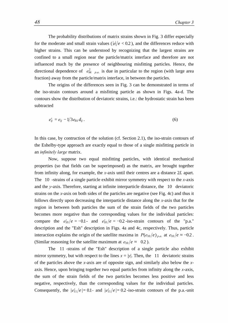
48 Chapter 3
The probability distributions of matrix strains shown in Fig. 3 differ especially
for the moderate and small strain values ( e ε < 0 2. ), and the differences reduce with
higher strains. This can be understood by recognizing that the largest strains are
confined to a small region near the particle/matrix interface and therefore are not
influenced much by the presence of neighbouring misfitting particles. Hence, the
directional dependence of ⟨ ⟩ehk p a2
. . is due in particular to the region (with large area
fraction) away from the particle/matrix interface, in between the particles.
The origins of the differences seen in Fig. 3 can be demonstrated in terms of
the iso-strain contours around a misfitting particle as shown in Figs. 4a-d. The
contours show the distribution of deviatoric strains, i.e.: the hydrostatic strain has been
subtracted
′ = −e e eij ij ij1 3 κκ δ . (6)
In this case, by contruction of the solution (cf. Section 2.1), the iso-strain contours of
the Eshelby-type approach are exactly equal to those of a single misfitting particle in
an infinitely large matrix.
Now, suppose two equal misfitting particles, with identical mechanical
properties (so that fields can be superimposed) as the matrix, are brought together
from infinity along, for example, the x-axis until their centres are a distance 2L apart.
The ⟨ ⟩10 -strains of a single particle exhibit mirror symmetry with respect to the x-axis
and the y-axis. Therefore, starting at infinite interparticle distance, the ⟨ ⟩10 deviatoric
strains on the x-axis on both sides of the particles are negative (see Fig. 4c) and thus it
follows directly upon decreasing the interparticle distance along the x-axis that for the
region in between both particles the sum of the strain fields of the two particles
becomes more negative than the corresponding values for the individual particles:
compare the ′ = −e10 01ε . - and ′ = −e10 0 2ε . -iso-strain contours of the "p.a."
description and the "Esh" description in Figs. 4a and 4c, respectively. Thus, particle
interaction explains the origin of the satellite maxima in P e p a( ) . .10 ε at e10 0 2ε ≈ − . .
(Similar reasoning for the satellite maximum at e10 0 2ε ≈ + . ).
The ⟨ ⟩11 -strains of the "Esh" description of a single particle also exhibit
mirror symmetry, but with respect to the lines x = |y|. Then, the ⟨ ⟩11 deviatoric strains
of the particles above the x-axis are of opposite sign, and similarly also below the x-
axis. Hence, upon bringing together two equal particles from infinity along the x-axis,
the sum of the strain fields of the two particles becomes less positive and less
negative, respectively, than the corresponding values for the individual particles.
Consequently, the | | .′ =e11 01ε - and | | .′ =e11 0 2ε -iso-strain contours of the p.a.-unit

X-Ray Diffraction Line Shift and Broadening of Precipitating Alloys; Part II 49
cell description are confined more to the particle than those of the Eshelby-type
description; cf. Figs. 4b and 4d. Therefore, the fraction of the p.a.-unit cell with ⟨ ⟩11
strains deviating only slightly from the average matrix strain (say, | | .′ <e11 01ε ) is
larger than for the "Esh" description. As a result, satellite maxima are absent for
P e p a( ) . .11 .
-0.50
-0.25
0
0.25
0.50
y/2L
-0.50 -0.25 0 0.25 0.50
x/2L
0
0
0
0.1 0.2
0.4 0
_
+
_
-0.50
-0.25
0
0.25
0.50
y/2L
-0.50 -0.25 0 0.25 0.50
x/2L
0.2 0.1
0
0
0 0
_+
+_
a) p.a-unit cell: ′e10 ε b) p.a-unit cell: ′e11 ε
-0.50
-0.25
0
0.25
0.50
y/2L
0.500.250-0.25-0.50
x/2L
0.4
0.2
0.1
0
0 0
0
_
+
_
-0.50
-0.25
0
0.25
0.50
y/2L
0.500.250-0.25-0.50
x/2L
0.4 0.2
0.1
0
0
0
_
+_
0
c) "Esh"-description: ′e10 ε d) "Esh"-description: ′e11 ε
Fig. 4. Comparison between the iso-strain contour plots of the ⟨ ⟩10 and ⟨ ⟩11 strain
distributions at a particle fraction c = 0.087, according to the p.a.-unit cell
description (Figs. a and b, respectively) and according to the Eshelby-type
description (Figs. c and d, respectively). Contour levels are | |′e ε = 0, 0.1, 0.2, 0.4
and 0.6 with signs as indicated. These figures show the deviatoric strains, see Eq. (6).

50 Chapter 3
4.2 Role of particle/matrix misfit; scaling properties
The calculated local strain scales linearly with the particle/matrix misfit ε, since linear
elasticity theory has been applied. Therefore, the probability distribution of matrix
strains, P ehk( )ε , is independent of ε and the average strains or the root mean
squared strains, ⟨ ⟩ehk2 , depend linearly on ε with proportionality factors determined
by c, E Ep m , νm and νp.
For equal Poisson ratios of particle and matrix (νm = νp = ν) the strain fields in
matrix and precipitate according to the Eshelby-type description are completely given
by a combination of ε and E Ep m through an effective misfit strain
ε εeff p mQ E E c= ( , ) (see appendix B). Hence ⟨ ⟩e Esh , ⟨ ⟩ehk Esh2 and the shape of the
probability distribution of matrix strains P ehk( )ε Esh depend on εeff only. Such kind
of scaling of the strain field (measures) also holds for the p.a.-unit cell description as
long as ⟨ ⟩ ≅ ⟨ ⟩e eEsh p a. . (see Fig. 1).
4.3 Role of particle clustering
The effect of clustering of misfitting particles on the strain parameters is analysed for
two different particle fractions, c = 0.031 and c = 0.087, corresponding to cases with a
relatively weak and relatively strong orientation dependence, respectively.
The strain fields of the large (4 4L L× ; cf. Fig. 2 in part I) p.a.-unit cells have
been calculated for cluster factors 0 < Cf < 0.5 for c = 0.087, and 0 < Cf < 0.7 for
c = 0.031 with E Ep m = 0.1, 1, and 10 (for definition of Cf, see Section 2.1 in part I).
Note that for any value of c there is an upper bound for Cf, recognizing impenetrable
particles: with L Rp p≥ 2 it follows C cf ≤ −1 2 π . Obviously, the strain field
according to the "Esh" description is independent of the cluster factor Cf (see Section
2.2). The p.a.-unit cell containing four particles exhibits the same symmetry properties
as the p.a.-unit cell containing a single particle and therefore the mean matrix strain of
the large p.a.-unit cell is also independent of direction (see Section 3). The average
matrix strain ⟨ ⟩e p a. . exhibits a very weak dependence on the cluster factor Cf for both
particle fractions. The relative difference between ⟨ ⟩e p a. . in the unclustered state
(Cf = 0) (practically equal to ⟨ ⟩e Esh ; see Section 4.1) and ⟨ ⟩e p a. . in the strongly
clustered state (Cf = 0.5 for c = 0.087 or Cf = 0.7 for c = 0.031) remains smaller than
0.2 % for E Ep m = 0.1 and E Ep m = 1, and increases to about 1 % if E Ep m = 10.
Therefore, it is concluded that the influence of clustering of misfitting particles on the
average matrix strain remains small.

X-Ray Diffraction Line Shift and Broadening of Precipitating Alloys; Part II 51
0.10
0.08
0.06
0.04
0.02
0
0.50.40.30.20.10Cf
Ep /Em = 10 Ep /Em = 1 Ep /Em = 0.1
<10>
<11>
<11>
<10>
Esh
Esh
<11>
<10>
Esh
Fig. 5. Normalised mean square strain ⟨ ⟩ehk2 2/ ε in the matrix, according to the p.a.-
unit cell description and according to the Eshelby-type description, versus
clusterfactor Cf for different values of E Ep m in two crystallographic directions,
⟨ ⟩10 and ⟨ ⟩11 , at constant c = 0.087.
0.4
0.3
0.2
0.1
0
P(ehk/ε)
-1.0 -0.5 0 0.5 1.0ehk/ε
<e10> <e11> Esh
<e>
Fig. 6. Probability distributions of matrix strains P(ehk/ε) in the ⟨ ⟩10 and ⟨ ⟩11
directions of normalised strain ehk/ε, according to the p.a.-unit cell description and
according to the Eshelby-type description, for a particle fraction of c = 0.087 with
E Ep m = 1 in the most clustered state considered, Cf = 0.5. The average matrix
strain is ⟨ ⟩ ≅ ⟨ ⟩ =e ep a Esh. . ε ε 0.032.
⟨ ⟩ehk2 2ε

52 Chapter 3
The mean squared strains are depicted in Fig. 5 as a function of the cluster
factor Cf for the case of c = 0.087 and E Ep m = 0.1, 1 and 10. As clustering becomes
more pronounced ⟨ ⟩e p a102
. . increases, whereas ⟨ ⟩e p a112
. . decreases (with approximately
the same amount). Similar behaviour is observed for c = 0.031, but less distinct. The
increase of the difference between ⟨ ⟩e p a102
. . and ⟨ ⟩e p a112
. . implies that the orientation
dependence becomes more pronounced for increasing clustering. This can also be seen
in the probability distribution of matrix strains that is shown for c = 0.087 and Cf = 0.5
in Fig. 6. As compared to the unclustered state (cf. Fig. 3), for P e p a( ) . .11 ε the
contribution of the strains close to zero has increased significantly, and the probability
distribution has become narrower as exhibited by the smaller value for the variance
⟨ ⟩e p a112
. . (see Fig. 5). As compared to the unclustered state P e p a( ) . .10 ε has become
broader, since the contribution of the shoulder at e ε ≈ 0 3. has become more
pronounced; see also the increase of ⟨ ⟩e p a102
. . with increasing Cf (Fig. 5).
0.50
0.25
0
y/4L
0.500.250
x/4L
0.4
0.2 0.1
0
0
0
+
__
+ 0
0.50
0.25
0
y/4L
0.500.250
x/4L
0
0
0
0
-0.1
-0.2
-0.4 -0.6
Fig. 7. Comparison between the iso-strain contour plots of the ⟨ ⟩10 and ⟨ ⟩11 strain
distributions with Cf = 0.5 at a particle fraction c = 0.087 for a quarter of a p.a.-unit
cell. Contour levels are | |′e ε = 0, 0.1, 0.2, 0.4 and 0.6 with signs as indicated. These
figures show the deviatoric strains, see Eq. (6).
The ⟨ ⟩10 and ⟨ ⟩11 iso-strain contour plots for a quarter of the large p.a.-unit
cell ( 4 4L L× ; cf. part I) in the most clustered state considered, Cf = 0.5 with
c = 0.087, are presented in Figs. 7a and 7b. The effects of clustering are clearly visible
upon comparing these figures with Figs. 4a and b for the unclustered state. Due to
clustering, the shape and symmetry properties of the strain field change. In particular,
in between the clustered particles, significant interaction distorts the strain
distribution.
′e10 ε
a)
′e11 ε
b)

X-Ray Diffraction Line Shift and Broadening of Precipitating Alloys; Part II 53
5. Line-Profile Calculations
In line with the previous discussion of the strain distributions {h0} and {hh} matrix
diffraction line profiles have been computed for values of the particle-matrix misfit εbetween 0 % and 5 %. For each series of line-profile simulations, line profiles have
been calculated for three orders of reflection (i.e. {10}, {20}, {30} and {11}, {22},
{33}).
5.1 Role of mechanical properties
The effect of the mechanical properties of particle and matrix on ⟨ ⟩ehk XRD and S hkε
has been studied by varying ε for constant values of Ep/Em (= 0.1, 1 and 10) and
c = 0.087. The simulations have used 2 2N N× = 240 240× atoms per p.a.-unit cell,
which corresponds to a particle radius of NR = 40 (cf. Section 2.2.1 of part I).
2.5x10⁻³
2.0
1.5
1.0
0.5
0
0.050.040.030.020.010ε
Ep/Em = 10 Ep/Em = 1 Ep/Em = 0.1
p.a, Esh
p.a, Esh
p.a, Esh
{h0} {hh}
{h0} {hh}
{hh} {h0}
Fig. 8a. The average matrix strains as a function of ε for the three values of Ep/Em for
c = 0.0873 and 2 2 240 240N N× = × . The average strains ⟨ ⟩ehk XRD have been
calculated from the centroid shift of the {hk} reflections. These strains can be
compared with ⟨ ⟩e p a. . calculated from the p.a-unit cell strain field, and with ⟨ ⟩e Esh
calculated from the approximate analytical strain field. The mean strains ⟨ ⟩e p a. . and
⟨ ⟩e Esh are independent of {hk} and practically equal (see text).
⟨ ⟩
⟨ ⟩
⟨ ⟩
e
e
e
hk XRD
hk Esh
hk p a. .

54 Chapter 3
2.5x10⁻³
2.0
1.5
1.0
0.5
0
2.5x10⁻³
2.01.51.00.50
Ep/Em = 10 Ep/Em = 1 Ep/Em = 0.1
Fig. 8b. The average matrix strains derived from the line profiles, ⟨ ⟩ehk XRD , versus
the average matrix strain, according the the p.a.-unit cell description, ⟨ ⟩e p a. . .
50x10-3
40
30
20
10
0
0.150.100.050
Ep/Em = 10 Ep/Em = 1 Ep/Em = 0.1 {h0}
{h0}
{h0}
{hh}
{hh}
{hh}
Fig. 8c. The standard deviation of the strain contribution to the broadening of the
{hk} reflection, S hkε , as a function of εHc
hk,0 .
⟨ ⟩ehk XRD
S hkε
⟨ ⟩e p a. .
εHchk,0

X-Ray Diffraction Line Shift and Broadening of Precipitating Alloys; Part II 55
50x10-3
40
30
20
10
0
50x10-3
403020100
Ep/Em = 10 Ep/Em = 1 Ep/Em = 0.1
Fig. 8d. The standard deviation of the strain contribution to the broadening of the {hk}
reflection, S hkε , as function of ⟨ ⟩e Hhk p a c
hk20. . , .
The variation of ⟨ ⟩ehk XRD with ε is shown in Fig. 8a, together with
corresponding curves for ⟨ ⟩e p a. . and ⟨ ⟩e Esh calculated according to Section 3.1.
Clearly, for all cases, ⟨ ⟩ehk XRD increases with ε in a nonlinear fashion while ⟨ ⟩e p a. .
and ⟨ ⟩e Esh scale linearly with ε. The ⟨ ⟩hk dependence of ⟨ ⟩ehk XRD -curves, for a
specific value of Ep/Em, is weak. Plotting ⟨ ⟩ehk XRD versus ⟨ ⟩e p a. . for all sets of
⟨ ⟩ehk XRD -curves (see Fig. 8b) shows that ⟨ ⟩ ⟨ ⟩e ehk XRD hk p a. . is practically
independent of Ep/Em. The systematic difference between ⟨ ⟩ehk XRD and ⟨ ⟩e p a. . will be
discussed in Section 5.5.
The variation of S hkε withεHc
hk,0 is shown in Fig. 8c. As compared to Fig. 8a,
εHchk,0 is used as abscissa instead of ε, to account for the dependence on the order of
reflection (cf. Eq. (5)). An almost linear dependence of S hkε on εHc
hk,0 is observed5.
The strain broadening strongly depends on the diffraction direction ⟨ ⟩hk and on
Ep/Em. Since ⟨ ⟩ehk p a2
. . scales with ε and Ep/Em (cf. Section 4.2), the linear
dependence of S hkε on εHc
hk,0 in Fig. 8c suggests that S hk
ε is roughly proportional with
5 Small deviations of linearity observed for 0 0 020≤ ≤εHcentr
hk, . , and in particular for small
2 2N N× (not shown here), are attributed to truncation of tails of the intensity distribution: overlapwith neighbouring reflections is more pronounced.
⟨ ⟩e Hhk p a chk2
0. . ,
S hkε

56 Chapter 3
⟨ ⟩ehk p a2
. . . As shown in Fig. 8d, this holds indeed: S hkε is proportional with
⟨ ⟩e Hhk p a chk2
0. . , , for all values of Ep/Em (see discussion in Section 5.5).
5.2 Role of particle fraction
The dependences of ⟨ ⟩ehk XRD and S hkε on ε have been studied for various values of
the particle fraction c for Ep/Em = 10 and NR = 40. In order that the particle size NR
remains constant, while c is varied, the number of atoms within a p.a.-unit cell,
2 2N N× , has been changed accordingly.
The results of the line profile calculations are presented in Figs. 9a and 9b.
Obviously, the slope of each set of ⟨ ⟩ehk XRD vs ε lines and each set of S hkε vs εHc
hk,0
lines increases with c, because the number of particles per unit area and thus the
deformation of the matrix increases with c, while the particle size remains constant.
Similar increases with c have been observed for ⟨ ⟩ehk p a. . and ⟨ ⟩ehk p a2
. . in Figs. 1
and 2, respectively. Indeed, plotting of ⟨ ⟩ehk XRD vs ⟨ ⟩ehk p a. . and S hkε vs
⟨ ⟩e Hhk p a chk2
0. . , for various values of c the same relations are observed as in Figs. 8b
and 8d, respectively.
5.3 Role of p.a.-unit cell size
The influence of the p.a.-unit cell size on ⟨ ⟩ehk XRD and S hkε is studied as a function of
ε for the {11} reflection and with Ep/Em = 1 and c = 0.087. An increase in the p.a.-unit
cell size 2 2L L× at constant a and c implies an enlargement of 2 2N N× and 2NR.
The results of this series of line profile calculations are presented in Figs. 10a
and 10b. It is important to note that since the displacements are sampled from a
continuum displacement field, the differences in position and width of the intensity
distribution for different 2L are a result of the diffraction process only.
However, it has been shown in part I that "size" broadening of a line profile
(as observed at ε = 0) depends on the distances in the matrix between the particles,
which at constant c are proportional to 2N (part I; Section 3.4). Therefore S hkε at ε = 0
is distinctly different for different 2N (see Fig. 10b). Thus, it can be expected that the
influence of the number of atoms in the p.a.-unit cell on the mean matrix strain as
function of ε and on the slope of the strain standard deviation as function of εHchk,0 is
small. This is confirmed by the results in Figs. 10a and 10b. As, for increasing 2N, the
strain field within the p.a.-unit cell is sampled at an increasing number of locations,
minor differences in ⟨ ⟩ehk XRD and S hkε can occur as a consequence of differences in
the sampling density.

X-Ray Diffraction Line Shift and Broadening of Precipitating Alloys; Part II 57
10.0x10⁻³
7.5
5.0
2.5
0
0.050.040.030.020.010ε
c = 0.401 c = 0.196 c = 0.0873
p.a Esh {h0} {hh}
p.a, Esh
p.a, Esh
{h0}
{h0} {hh}
{hh}
Fig. 9a. The average matrix strains, ⟨ ⟩ehk XRD , ⟨ ⟩e p a. . and ⟨ ⟩e Esh , as a function of εfor the three values of c for Ep/Em = 10 and NR = 40. See also caption of Fig. 8.
100x10-3
80
60
40
20
0
0.150.100.050
{h0}
{h0}
{h0}
{hh}
c = 0.401c = 0.196c = 0.0873
{hh}{hh}
Fig. 9b. The standard deviation of the strain contribution to the broadening of the {hk}
reflection, S hkε , for three values of c for Ep/Em = 10 and NR = 40 as a function of
εHchk,0 .
εHchk,0
S hkε
⟨ ⟩
⟨ ⟩
⟨ ⟩
e
e
e
XRD
Esh
p a. .

58 Chapter 3
1.5x10⁻³
1.0
0.5
0
0.050.040.030.020.010ε
2N = 602N = 1202N = 2402N = 480
Fig. 10a. The average matrix strain, ⟨ ⟩e XRD11 as a function of ε for four values of
2 2N N× for c = 0.0873. See also caption of Fig. 8.
40x10-3
20
0
-20
0.150.100.050
2N = 60
2N = 120
2N = 240
2N = 480
{h0}
{hh}
Fig. 10b. The standard deviation of the strain contribution to the broadening of the
{hk} reflection, S hkε , for four values of 2 2N N× as a function of εHc
hk,0 for
c = 0.0873. The dependence of S hkε on {hk} is the same for all values of 2N .
ε εH hk,0
S hkε
⟨ ⟩e XRD11

X-Ray Diffraction Line Shift and Broadening of Precipitating Alloys; Part II 59
5.4 Role of clustering
The influence of clustering of the particles on ⟨ ⟩ehk XRD is very small. Only in the most
clustered state considered with Cf = 0.5 and with Ep/Em = 10, c = 0.087 and
4 4N N× = 240 240× a difference of about 1.1 % is observed in ⟨ ⟩e XRD11 .
The effect of clustering becomes clearly visible, however, in S hkε . For
example, it follows from Fig. 11a that Sstrain33 decreases significantly due to clustering.
Yet, again plotting Sε33 vs ⟨ ⟩e Hp a c33
20
33. . , yields a straight line (cf. Figs. 8d and 11b),
also in the present clustered state.
5.5 Concluding remarks on line profile centroid and variance
The relation between line width and ⟨ ⟩e Hhk p a chk2
0. . , (cf. Eq. 5) has been studied
extensively in Ref. [11] for a material containing a distribution of defects, such as
dislocations or misfitting particles. It was shown that the type and the distribution of
defects within a material determine this relation. In case of a periodic distribution of
defects, each associated with the same type of strain field (Cauchy-type: ε ~ 1/r2, with
r the distance from the defect, a possible approximative model for screw dislocations)
it followed that there was a linear relation between the integral breadth, as a measure
of line-profile width, and ⟨ ⟩e Hhk p a chk2
0. . , . The present work demonstrates that a
similar result holds for misfitting particles (based on an exact elaboration of the
misfit-strain fields).
Minor effects such as (i) the nonlinear dependence of ⟨ ⟩ehk XRD on ⟨ ⟩e p a. . and
(ii) the departure of the slope of S hkε vs ⟨ ⟩e Hhk p a c
hk20. . , -lines from unity (cf. Eqs. 4
and 5) can be understood as true effects made visible here due to the exact calculation
of the diffracted intensity, thereby avoiding approximations that are usually made (e.g.
[1, 12]).
In diffraction calculations two simplifications are commonly made6:
(i) The inner product of the diffraction vector H with the vector indicating the
displacement of each atom (mn) is approximated by the length of the diffraction
vector indicating the Bragg reflection of the reflection considered, HB, and the
component of the displacement field of atom mn in the direction of HB.
(ii) The usual procedure to obtain a powder diffraction line profile from the
intensity distribution in reciprocal space of a single powder particle employs the so-
6 In textbooks on X-ray diffraction (e.g. Warren [1]) this approximation is carried out by replacing thecontinous variable in reciprocal space, h3, by the order of reflection, l, of a {00l}-type reflection andtaking the component of the displacement of unit cell m along the h3-axis, Zm.

60 Chapter 3
50x10-3
40
30
20
10
0
0.150.100.050
Ep/Em = 10 Ep/Em = 1 Ep/Em = 0.1
Cf = 0
Cf = 0.5
Cf = 0
Cf = 0.5
Cf = 0.5
Cf = 0
Fig. 11a. The standard deviation of the strain contribution to the broadening of the
{33} reflection, Sε33 , for two values of Cf as a function of εHc,0
33 for c = 0.0873.
50x10-3
40
30
20
10
0
50x10-3
403020100
Ep/Em = 10 Ep/Em = 1 Ep/Em = 0.1
Fig. 11b. The standard deviation of the strain contribution to the broadening of the
{33} reflection, Sε33 , as a function of ⟨ ⟩e Hp a c33
20
33. . , for c = 0.0873 with Cf = 0 or
Cf = 0.5.
Sε33
εHc,033
⟨ ⟩e Hp a c332
033
. . ,
Sε33

X-Ray Diffraction Line Shift and Broadening of Precipitating Alloys; Part II 61
called tangent plane approximation instead of the rotation procedure as used in this
work (see Section 2.2.3 in part I).
These effects are illustrated in Figs. 12a and 12b showing exact and
approximate results for ⟨ ⟩ehk XRD and S hkε of a {33} reflection, calculated for the case
of an unclustered p.a.-unit cell with Ep/Em = 1, c = 0.087, 2 2N N× = 60 60× and
ε = 0 to 0.05. The intensity distribution calculated using the approximation (i) deviates
from the exact one far away from the position of the matrix Bragg reflection in
reciprocal space. The exact calculation of the diffracted intensity shows a slight
asymmetry for the tails of the powder diffraction line profile, in particular for
increasing values of ε. This causes ⟨ ⟩ehk XRD to be nonlinearly dependent on ε and
thus ⟨ ⟩ehk p a. . (see Figs. 8b, 9b, 10a).
The consequence of the use of the tangent plane approximation (i.e.
approximation (ii)) is visible also in Fig. 12a. The larger the broadening the larger the
influence of this approximation (see also discussion in part I).
2.0x10⁻³
1.5
1.0
0.5
0.0
2.0x10⁻³
1.51.00.50.0
} approx
} exact
Fig. 12a. Average matrix strains calculated from {33} diffraction-line profiles as a
function of the average matrix strain according to the p.a.-unit cell description,
⟨ ⟩e p a33 . . for Ep/Em = 1, c = 0.087, 2 2N N× = 60 60× and ε = 0 - 0.05. The {33}
line profiles have been calculated applying either the exact formulae leading to,
⟨ ⟩e XRD33 , or the approximate formulae for the intensity distribution in reciprocal
space, leading to ⟨ ⟩e XRDapprox
33 (see text); these intensity distributions have been
subsequently projected on the diffraction vector either by the tangent procedure
(dashed line) or the rotation procedure (solid line).
⟨ ⟩e p a33 . .
⟨ ⟩
⟨ ⟩
e
e
XRD
XRDapprox

62 Chapter 3
40x10-3
30
20
10
0
40x10-3
3020100
approx exact
Fig. 12b. Sε33 and S approx
ε33 as a function of ⟨ ⟩e Hp a c33
20
33. . , . See caption of analogous
Fig. 12 a.
As both approximations influence in particular the asymmetry in the observed
intensity distribution, albeit slightly, the effect on the centroid is larger than on the
variance. This can be understood as follows. If the intensity distribution is divided into
an even part and an uneven part with respect to the position of the Bragg reflection
considered, then it follows from Eqs. (2) and (3) that the centroid is sensitive to the
uneven part of the intensity distribution, whereas the variance is, to a large extent,
sensitive to the even part of the intensity distribution; a small effect of the uneven part
on the variance remains since the variance is determined with respect to the centroid,
cf. Eq. (3). Therefore, the influence of the approximations used is most clearly visible
in the centroid of the intensity distribution.
6. Conclusions
(i) The mean strain of, and the centroid of a diffraction line profile from, an isotropic
matrix containing circular misfitting inclusions, that are not severely clustered, can be
well calculated adopting an Eshelby-type description for the strain field of a single
⟨ ⟩e Hp a c332
033
. . ,
S
S approx
ε
ε
33
33

X-Ray Diffraction Line Shift and Broadening of Precipitating Alloys; Part II 63
misfitting particle, i.e. ignoring particle misfit-strain field interaction and using an
effective radius for the matrix surrounding the single particle.
(ii) The probability distribution of matrix strains and the diffraction-line broadening
due to strain cannot be calculated reliably from an Eshelby-type approach. More
accurate calculations of the strain field in the matrix may be required, for example
using a finite element analysis.
(iii) The centroid of a diffraction line profile of the matrix is practically linearly
related to the mean strain of the matrix.
(iv) The strain broadening in reciprocal space of a diffraction-line profile of the matrix
is practically linearly related to the product of the linear misfit of particle and matrix
and the order of reflection. The standard deviation of the only strain broadened part of
the intensity distribution (in reciprocal space), as a measure of line profile width,
equals, to a high degree of accuracy, the product of the mean square strain in the
direction of the diffraction vector and the centroid of the intensity distribution.
(vi) Clustering of particles enhances the direction dependence of the root mean square
strain and the diffraction-line broadening significantly, but the mean strain and the
centroid of the diffraction line profile are hardly affected.
Acknowledgement
This work has been part of the research program of the Foundation for Fundamental
Research on Matter (Stichting FOM), The Netherlands.
Appendix ADirectional independence of mean matrix strain ⟨ ⟩ehk p.a.
The mean strain in the matrix in the direction of an arbitrary vector n = (cos , sin )φ φ ,
determined by the angle φ , as defined in Fig. A. 1, is equal to
⟨ ⟩ =∫∫
∫∫e
e x y dxdy
dxdyA
A
m
m
n
n ( , )
(A. 1)
with Am the matrix part of the p.a.-unit cell and with e x yn ( , ) the strain in the
direction of n at location (x,y), which is related to the components εij of the strain
tensor by

64 Chapter 3
ε ε φ ε φ φ ε φn = + +112
12 2222cos cos sin sin . (A. 2)
If the strain tensor at every position in the matrix is known, the mean strain is
readily calculated from Eqs. (A. 1) and (A. 2). However, using the symmetry
properties of the p.a.-unit cell it can be shown that the mean matrix strain is
independent of the direction of n and equal to the hydrostatic strain of the matrix.
Therefore, the mean matrix strain is now calculated by separating the calculation into
(i) the determination of the average strain of a set of selected points and (ii) the
integration over all such sets. An example of a set of selected points A, B, C and D is
shown schematicly in Fig. A.1. If the strain tensor is known at A, the strain tensors in
points B, C and D (cf. Fig. A.1), located symmetrically with respect to the symmetry
lines x = 0 and x = |y|, are related to the strain tensor in point A by
B
C
D
B A B A B A
C A C A C A
D A D A D A
: ; ;
: ; ;
: ; ;
ε ε ε ε ε ε
ε ε ε ε ε ε
ε ε ε ε ε ε
11 22 22 11 12 12
11 22 22 11 12 12
11 22 22 11 12 12
= = =
= = = −
= = = −
(A. 3)
φ
x = y x = -y
A
B C
D
n
x
y
Fig. A.1. Schematic drawing of the p.a.-unit cell and symmetry lines x = 0, y = 0 and
x = |y|. Point B is located symmetrically to A with respect to x = –y. Points C and D
are located symmetrically to B and A, respectively, with respect to x = 0. The angle
between the x-axis and an arbitrary unit vector n is defined as φ. The directions of the
shear components of the strain tensors in the points A, B, C and D are indicated.

X-Ray Diffraction Line Shift and Broadening of Precipitating Alloys; Part II 65
The average strain of this set of points in the direction of n is equal to:
⟨ ⟩ = +e ABCDA A
n1
2 11 22( )ε ε (A. 4)
which is equal to the hydrostatic strain in A, B, C and D.
Subsequently, the mean matrix strain follows from averaging over the results
of all sets of points such that the entire matrix of the p.a.-unit cell is covered. Since for
all other sets the average strain is also independent of n and equal to the hydrostatic
strain in the points considered, the mean matrix strain ⟨ ⟩e is (i) independent of the
direction of n, and thus independent of the diffraction direction ⟨ ⟩hk and (ii) equal to
the hydrostatic strain of the entire matrix of the p.a.-unit cell.
Appendix BStrain field for circular inclusion in circular matrix
The components of the rotationally symmetric strain field in particle and matrix, εr, εt,
εrt = εtr = 0 (r and t denoting the radial and tangential directions, respectively)
pertaining to a misfitting circular particle (radius Rp, Young's modulus Ep, Poisson's
ratio νp) placed centrally in a circular matrix (radius Rm > Rp, Young's modulus Em,
Poisson's ratio νm) are given in Ref. [13]. The derivation is limited to the case where
νm = νp = ν.
The strain field in the precipitate ( r Rp≤ ) is uniform and can be written as
ε ε εrp
tp
p mQ E E c= = ( , ) , (B. 1)
where c R Rp m= 2 2 and ε denotes the linear misfit at the particle/matrix interface and
where
( ){ }( )
{ }( ) ( )( )QE
Ec
E E c c
E E c cp
m
p m
p m( , ) =
+−
+ −− + + −
− + − − −
12
11
1 1 21 2 1 1
1 2 1 1 2 1
νν
νν
ν ν.
(B. 2)
The strain components in the matrix read ( R r Rp m< ≤ )

66 Chapter 3
ε εν
νrm
rp p
rc R r
c( )
( )
( )=
− −− +
1 2
1 2 1
2 2
, (B. 3)
ε εν
νtm
rp p
rc R r
c( )
( )
( )=
− +− +
1 2
1 2 1
2 2
. (B. 4)
The strain components in the matrix depend linearly on ε through the precipitate strain
ε rp given in Eq. (B. 1). Therefore, an effective linear misfit parameter ε eff can be
defined as follows
ε ε ε εeff rp
tp
p mQ E E c= = = ( , ) . (B.5)
References
[1] B.E. Warren, X-ray Diffraction, Reading, Massachusetts: Addison-Wesley, 1969.
[2] M.A. Krivoglaz, X-ray and Neutron Diffraction in Nonideal Crystals, Springer, 1996.
[3] E.J. Mittemeijer, P. van Mourik, Th.H. de Keijser, Phil. Mag. 43 (5), (1981), 1157 - 1164.
[4] T.C. Bor, R. Delhez, E.J. Mittemeijer, E. Van der Giessen, Mat. Sci. & Eng. A234-236
(1997) 896 - 899.
[5] T.C. Bor, R. Delhez, E.J. Mittemeijer, E. Van der Giessen, in Proc. 5th Int. Conf.
Residual Stresses, Eds. T. Ericsson, M. Odén, A. Andersson, Linköping University, (1997)
592 - 597.
[6] J.D. Eshelby, Solid State Phys. 3 (1956), 79 - 144.
[7] O.C. Zienkiewics, The Finite Element Method in Engineering Science, McGraw-Hill,
London, 1971.
[8] A.J.C. Wilson, Proc. Phys. Soc. 80, 286 - 294, 1962.
[9] A.J.C. Wilson, Proc. Phys. Soc. 81, 41 - 46, 1963.
[10] J.I. Langford, A.J.C. Wilson, In: Crystallography and Crystal Perfection, ed. G.N.
Ramachandran, Academic Press, London, 207 - 222 (1963).
[11] J.G.M. van Berkum, R. Delhez, Th.H. de Keijser, E.J. Mittemeijer, Acta Cryst. A52
(1996) 730 - 747.
[12] A.J.C. Wilson, Elements of X-ray Crystallography, Addison-Wesley, Reading,
Massachusetts (1970).
[13] S.P. Timoshenko and J.N. Goodier, Theory of Elasticity, 3rd edn., McGraw-Hill, New
York (1970).
Chapter 4
Diffraction Contrast Analysis of Misfit Strainsaround Inclusions in a Matrix
VN Particles in α-Fe
T.C. Bor1,3, A.T.W. Kempen2, F.D. Tichelaar1,
E.J. Mittemeijer1,2 and E. Van der Giessen3
1Laboratory of Materials Science, Delft University of Technology,
Rotterdamseweg 137, 2628 AL Delft, The Netherlands2Max Planck Institute for Metals Research,
Seestraße 92, 70174 Stuttgart, Germany3Koiter Institute Delft, Delft Universiy of Technology,
Mekelweg 2, 2628 CD Delft, The Netherlands
Abstract
A new method has been developed to determine the misfit of disc-shaped precipitates in a
matrix using Transmission Electron Microscopy (TEM). The method is applicable to
specimens containing a high precipitate density, where the classical TEM method, based on
the extent of the precipitate diffraction contrast cannot be applied. The new method is based
on evaluation of the positions of extrema in the intensity distribution due to misfitting
precipitates both in bright field and dark field. A model system, consisting of a single disc-
shaped misfitting precipitate placed centrally in a thin specimen, has been studied first. The
dynamical theory of electron diffraction has been adopted for a four beam case. The contrast
lobes in bright and dark field images have been calculated as a function of, in particular, the
particle radius, the foil thickness and the particle thickness. Simultaneous fitting of calculated
bright and dark field diffraction contrast images to the experimental ones leads to
determination of the precipitate misfit, and the local thickness of the specimen foil. The
method has been illustrated for a nitrided Fe-2 at. % V alloy with small disc-shaped VN
precipitates and has led to a consistent interpretation in terms of particle size and misfit upon
precipitation. The extent of elastic accommodation of misfit has been verified using High
Resolution Electron Microscopy (HREM). The foil thickness values determined by
diffraction contrast analysis agree well with independently obtained corresponding data. In
addition X-Ray Diffraction (XRD) line profiles of the specimes have been recorded. The
observed shifts and broadenings of the XRD profiles support the results obtained using TEM.

68 Chapter 4
1. Introduction
Small misfitting particles/precipitates in a matrix can enhance the mechanical
properties to a large extent. The increases of, for example, the yield strength and
hardness are dependent on the size and shape of the precipitate particles and, in
particular, on the (volume) misfit between the matrix and the particle [1]. This
particle-matrix misfit causes a strain field in both the particle and the matrix that
influences the motion of dislocations. To understand material behaviour it is therefore
important to obtain quantitative information about the size, the shape and the misfit of
the particles introduced.
Several experimental techniques exist that enable the study of small misfitting
particles in a matrix, from which Transmission Electron Microscopy (TEM) and X-
Ray Diffraction (XRD) are the most important ones. The particle-matrix strain field
causes deformation of the matrix lattice which in TEM gives rise to the appearance of
contrast lobes around the misfitting particle both in bright field (BF) and dark field
(DF) images [2,3]. In the case of XRD the position, the shape and the width of an
{hkl} line profile change [4, 5].
The classical method to obtain a quantitative estimate of the particle-matrix
misfit of spherical or disc-like particles using TEM is due to Ashby and Brown [2,3].
This method is based on measurement of the width of the contrast image with respect
to the intensity of the background. However, this method is unreliable, as shown in
this paper, for the determination of the particle-matrix misfit of particles located in
thin foils if (i) a foil thickness occurs smaller than approximately four to five times the
extinction distance (for such foils the influence of the foil thickness on the image
width cannot be neglected; see also Fig. 2) and/or if (ii) significant overlap occurs of
the contrast lobes of neighbouring misfitting particles and the intensity of the
background cannot be measured accurately.
The present work proposes and tests an alternative method that does not have
the limitations of the Ashby and Brown method. The strain contrast is characterized
by the distance of the maximum or minimum intensity of the contrast lobes in BF and
DF to the centre of the misfitting particle. Full BF and DF contrast images are
calculated and compared with experimental ones. Further, since it is often difficult to
realize a “two-beam” case of electron diffraction for thin specimen foils (as in the
earlier method), a more general “four-beam” case is adopted here.
The method has been applied to the case of a nitrided Fe-2 at.% V alloy
containing a high number density of small disc-shaped VN precipitate particles
exhibiting large misfit with the ferrite (α-Fe) matrix.

Diffraction Contrast Analysis of Misfit Strains… 69
2. Calculated BF and DF diffraction contrast images
2.1 Theoretical background
The calculation of the diffraction contrast of misfitting particles is carried out using
the following assumptions. (i) The strain field contrast can be adequately calculated
using the dynamical theory of electron diffraction considering a four beam case (cf.
Section 4.1). The theory is briefly presented in Section 2.1.1. (ii) The disc-like or
penny shaped particles are embedded in an elastically isotropic matrix with a misfit in
the direction perpendicular to the disc plane only; there is no misfit in the direction
parallel to the disc plane. (iii) It is assumed that the displacement field of one
misfitting particle in an infinitely large matrix is a sufficiently accurate description of
the displacement field close to a misfitting particle in a matrix having a high number
density of such particles. The displacement field is briefly presented in Section 2.1.2.
2.1.1 Dynamical theory of electron diffraction
The basis of the computation of the images in BF and DF is the dynamical theory of
diffraction contrast in the form developed by Howie and Whelan [6]. A specimen of
thickness t is divided into columns along the z-axis of an orthogonal xyz-coordinate
system, see Fig. 1. A four beam case is considered: Φ0, Φ–g, Φg and Φ2g indicate the
amplitudes of the direct beam and three diffracted beams. The diffraction vectors g, –g
and 2g are perpendicular to the z-axis. The coupling of Φ0, Φ–g, Φg and Φ2g as a
function of depth z in the crystal is described by the following coupled differential
equations [6, 7]
d
dzi
i s s zk
j kj
j j k j kΦ
Φg
g ggg g g g g u= − + − ⋅
−∑
πξ
πexp( [( ) ( ) ])2 . (1)
The change of each amplitude Φ gk in a thin slab of thickness dz, d dz
kΦ g with
gk = –g, 0, g and 2g for k = 1, 2, 3 and 4, consists of the sum of the contributions of all
four amplitudes. For each amplitude a phase factor depending on the deviations from
the Bragg positions, s–g, s0, sg, s2g, and on the displacement field caused by the
misfitting particle, u (see next Section), is taken into account. In these equationsξg gj k−
represents the complex extinction distance of gj – gk, i.e. of the "incident" beam gk that
diffracts towards the diffracted beam gj. The effect of inelastic scattering is
incorporated by replacing 1 ξg by 1 ξ ξg g+ ′i where g = gj – gk [2, 3, 7].

70 Chapter 4
The amplitudes at the bottom of the specimen are obtained by solving this set
of differential equations with the boundary conditions Φ0 = 1 and Φ–g = Φg = Φ2g = 0
at the top of the specimen. Subsequently, the amplitudes of each beam are multiplied
with their corresponding complex conjugates to yield the intensities.
R
+y
+z
VN
t
g
u
b
+x
Fig. 1. Sch
In order to simplify the calculation a location in the (distorted, experimental)
specimen is chosen within a bright bend contour in the dark field image obtained with
diffraction vector g. There, sg = 0 and s0 = 0 and s–g = s2g = s, where s follows from
straightforward geometric analysis in reciprocal space
smalldislocation loopat (x',y',z')
(x,y,z)
Fig. 1. Schematic drawing of a misfitting particle of radius R in the middle of a foil of
thickness t and located at the origin of an xyz-coordinate system. The misfitting
particle is represented by a collection of small prismatic dislocation loops with
Burgers vector b normal to the dislocation plane dy'dz'. Each such dislocation causes
a displacement field du within the matrix. The total displacement field at a point
(x,y,z) is equal to the sum of the contributions of all dislocation loops making up the
particle. The diffraction contrast images have been calculated dividing the specimen
into independently diffracting columns parallel to the z-axis. Each column represents
one pixel of the simulated image. Diffraction vector g is oriented perpendicularly to
the misfitting particle.

Diffraction Contrast Analysis of Misfit Strains… 71
s g g= −
− −
1 12
1 322
2
2
2
λ λ(2)
with λ the electron wavelength and g = |g|.
2.1.2 Displacement field of a misfitting particle
The displacement field induced in the matrix by a misfitting disc-shaped particle can
be calculated by representation of the particle by a collection of prismatic dislocation
loops placed parallel in the plane of the disc at the location of the disc in an infinitely
large matrix as shown schematically in Fig. 1 [2, 3] (matrix assumed to be elastically
isotropic; misfit only perpendicular to the disc). Each dislocation loop has an area
dy'dz' (disc parallel to z- and y- axes) and a Burgers vector b parallel to the loop
normal. Note that the operating diffraction vector is oriented perpendicularly to the
disc-shaped particle. This Burgers vector can be interpreted as follows: if the particle
(disc) consists of n lattice planes with interplanar distance dparthkl
and the matrix at the
location of the particle in its hypothetical absence would consist of an equal number of
lattice planes with interplanar distance dmatrh'k ' l' parallel to the lattice planes of the
particle/disc, then, if a coherent interface exists between the matrix and the particle,
the length of b equals
b n d dparthkl
matrh k l= −( )' ' ' (3a)
The thickness of the disc-shaped particle, tpart, is defined as t ndpart parthkl≡ . The relation
between tpart and b is then given by
td
d dbpart
parthkl
parthkl
matrh k l=
−( )' ' ' . (3b)
The interplanar distances of the lattice planes of the particle and the matrix, dparthkl and
dmatrh'k ' l' , respectively, are calculated straightforwardly from the respective lattice
constants of the particle and the matrix.
The elastic displacement field at a point (x,y,z) due to a single prismatic
dislocation loop located at (x',y',z') in an isotropic, infinitely large matrix with the
Burgers vector parallel to the x-axis is given by [8]

72 Chapter 4
( )
( )
( )
dubdy dz
rx x
rx x
r
dubdy dz
ry y
rx x y y
r
dubdy dz
rz z
rx x z z
r
x
y
z
=−
−−
+−
=−
−−
−− −
=−
−−
−− −
' '( )
( ' ) ( ' )
' '( )
( ' ) ( ' ) ( ' )
' '( )
( ' ) ( ' ) ( ' )
8 11 2 3
8 11 2 3
8 11 2 3
2
3
3
2
2
3
2
2
3
π νν
π νν
π νν
(4a)
with
r x x y y z z2 2 2 2= − + − + −( ' ) ( ' ) ( ' ) (4b)
and ν being Poisson's ratio. The total displacement field of the misfitting particle is
equal to the sum of the displacement fields of the individual prismatic dislocation
loops making up the particle with radius R,
u uzy'
= ∫∫ d'
(5)
In diffraction contrast calculations the displacement field is usually simplified
by splitting it up into a dilatation component and a rotation component [7]. The
contribution of the dilatation component to image contrast can be shown to be
negligibly small in TEM [7]. Therefore only the contribution of the rotation
component to image contrast is considered in this work.
2.1.3 Procedures of strain field contrast image calculation
The intensity distribution in a BF or DF image at the bottom of a sample has been
calculated using a modified version of the TEM software package SIMCON [9], that
has been adapted here to allow calculations for four beam cases. The specimen is
subdivided in independently diffracting columns perpendicular to the operating
diffraction vectors (cf. Section 2.1.1). Each column represents one pixel of the
simulated image. The size of the image (width times height) and the desired resolution
of the image, i.e. the number of pixels per nanometer, determine both the total number
of columns used for the specimen and the lateral size of each column (i.e. the size of
the column in the directions parallel to the x-axis and y-axis). For every column Eq.
(1) is solved numerically, with the displacement field according to Eqs. (4) and (5),
using a fifth-order Runge Kutta scheme [10] with a maximum relative integration
error of 1.10-6. In analogy with Howie and Whelan [6] the set of equations describing
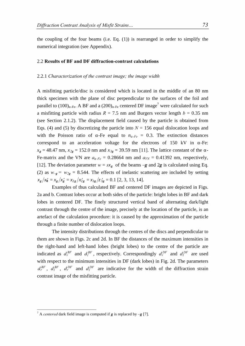
Diffraction Contrast Analysis of Misfit Strains… 73
the coupling of the four beams (i.e. Eq. (1)) is rearranged in order to simplify the
numerical integration (see Appendix).
2.2 Results of BF and DF diffraction-contrast calculations
2.2.1 Characterization of the contrast image; the image width
A misfitting particle/disc is considered which is located in the middle of an 80 nm
thick specimen with the plane of disc perpendicular to the surfaces of the foil and
parallel to (100)α-Fe. A BF and a (200)α-Fe centered DF image7 were calculated for such
a misfitting particle with radius R = 7.5 nm and Burgers vector length b = 0.35 nm
(see Section 2.1.2). The displacement field caused by the particle is obtained from
Eqs. (4) and (5) by discretizing the particle into N = 156 equal dislocation loops and
with the Poisson ratio of α-Fe equal to να-Fe = 0.3. The extinction distances
correspond to an acceleration voltage for the electrons of 150 kV in α-Fe:
ξg = 48.47 nm, ξ2g = 152.0 nm and ξ3g = 39.59 nm [11]. The lattice constant of the α-
Fe-matrix and the VN are aα-Fe = 0.28664 nm and aVN = 0.41392 nm, respectively,
[12]. The deviation parameter w = sξg of the beams –g and 2g is calculated using Eq.
(2) as w–g = w2g = 8.544. The effects of inelastic scattering are included by setting
ξ ξ ξ ξ ξ ξ ξ ζg g g g g g g′ = ′ = ′ = ′0 2 2 3 3 = 0.1 [2, 3, 13, 14].
Examples of thus calculated BF and centered DF images are depicted in Figs.
2a and b. Contrast lobes occur at both sides of the particle: bright lobes in BF and dark
lobes in centered DF. The finely structured vertical band of alternating dark/light
contrast through the centre of the image, precisely at the location of the particle, is an
artefact of the calculation procedure: it is caused by the approximation of the particle
through a finite number of dislocation loops.
The intensity distributions through the centres of the discs and perpendicular to
them are shown in Figs. 2c and 2d. In BF the distances of the maximum intensities in
the right-hand and left-hand lobes (bright lobes) to the centre of the particle are
indicated as drBF and d l
BF , respectively. Correspondingly drDF and d l
DF are used
with respect to the minimum intensities in DF (dark lobes) in Fig. 2d. The parameters
drBF , d l
BF , drDF and d l
DF are indicative for the width of the diffraction strain
contrast image of the misfitting particle.
7 A centered dark field image is computed if g is replaced by –g [7].

74 Chapter 4
(a) BF (b) centered DF
0.50
0.25
0Inte
nsity
(a.
u.)
-30 -20 -10 0 10 20 30(nm)
0.50
0.25
0
-30 -20 -10 0 10 20 30(nm)
(c) BF (d) centered DF
Fig. 2. Simulated BF (a) and (200)α-Fe centered DF (b) images of a misfitting VN
particle (disc) of radius R = 7.5 nm and Burgers vector b = 0.35 nm in the middle of a
80 nm thick α-Fe-foil with operating reflections ( 2 0 0)α-Fe, (000), (200)α-Fe and (400)α-
Fe. The image size is 75 75× nm2. Below each image the intensity distribution along a
horizontal line through the centre of the image is shown for the BF (c) and centered
DF (d) images. The particle-lobe distances for BF, d lBF and dr
BF , and centered DF,
d lDF and dr
DF , have been indicated. In addition, the image width in BF, defined
according to Ashby and Brown [2, 3] as the distance along the line through the centre
of the particle where the intensity differs more than 20 % of the background intensity,
d A B& , is depicted in Fig. 2c.
2.2.2 Parameters determining the image width
A number of simulations was carried out to investigate the influence of several
parameters on the DF and the BF images, such as the foil thickness, the particle/disc
radius, the effective particle thickness (i.e. the particle Burgers vector, see Section
d lBF dr
BF
d A B&

Diffraction Contrast Analysis of Misfit Strains… 75
2.1.2) and the depth location of the particle in the specimen foil. Subsequently, the
influence of a neighbouring particle on the image width was studied.
2.2.2.1 Foil thickness
The thickness of the foil, t, was varied from 50 nm to 200 nm in steps of 2.5 nm,
while the particle was positioned in the middle of the foil and the Burgers vector
length b and particle radius R were kept constant: b = 0.35 nm and R = 7.5 nm. The
distances dBF and dDF to the centre of the particle of each bright lobe in BF and each
dark lobe in DF, respectively, are shown in Fig. 3. The so-called 20 % image width in
BF, defined by Ashby and Brown [2, 3] as the distance along the line through the
centre of the particle where the intensity differs more than 20 % of the background
intensity, has also been indicated.
10
8
6
4
2
0 par
ticle
lobe
dis
tanc
e (n
m)
20015010050t (nm)
60
50
40
30
Fig. 3. Particle-lobe distance in BF images (bright lobe) and in (200)α-Fe centered DF
images (dark lobe) of a misfitting VN particle of radius R = 7.5 nm and Burgers
vector b = 3.5 nm, in the middle of an α-Fe foil as a function of foil thickness, t. Full
BF and centered DF images at each specimen thickness marked by the cross filled
circles on the abscissa are shown in Fig. 4. The image width, defined according to
Ashby and Brown [2, 3] as the distance along the line through the centre of the
particle where the intensity differs more than 20 % of the background intensity,
d A B& , is depicted as a function of the specimen thickness in the upper part.
drDFd BF d l
DF
d
nm
A B&
( )

76 Chapter 4
Clearly, the 20%-image width depends on the specimen/foil thickness, especially for t
< 100 nm ≈ 2ξg. Ashby and Brown did not consider the influence of the specimen/foil
thickness on the image width for foils with a foil thickness t < 3.5ξg. Application of
the Ashby and Brown method for cases with t < 4ξg (≈ 200 nm; note that electron
transparent foils are usually very much thinner), without more ado, will lead to
erroneous results in the determination of the particle Burgers vector.
The results of the particle-lobe distance parameters dBF and dDF show a zig-zag
dependence as a function of the foil thickness, which can be understood considering
the series of BF and corresponding centered DF images shown in Figs. 4a-e. These
series correspond to the abscis values indicated with ⊗ in Fig. 3. Starting at t = 50 nm
the lobes move away from the particle centre for increasing t, cf. for instance Fig. 4a
with Fig. 4b. At some thickness, approximately t = 100 nm in this case, a second
bright lobe in BF and a second dark lobe in centered DF appears in between the
particle and the first lobe, cf. Fig. 4c. The lobe closest to the particle has been used to
determine dBF and dDF and therefore a step occurs in Fig. 3 (compare Fig. 3 and Figs.
4b, 4c and 4d), etc.
Since the particle is positioned in the middle of the foil and the deviation from
the Bragg position of g is taken to be zero (cf. Section 2.1.1), the lobes of the BF
image are always symmetric: drBF = d l
BF . The centered DF images are usually
asymmetric: d drDF
lDF≠ . It depends on the value of t whether the right or left dark
lobe is closest to the particle in the DF image.
2.2.2.2 Particle radius
The influence of the particle radius on the extent of the contrast lobes in BF and DF is
shown in Fig. 5 for a 80 nm thick specimen. On increasing the particle radius the
lobes move away from the particle. Below R = 2.5 nm it is difficult or impossible to
find a bright lobe for the BF images and a dark lobe for the centered DF images on
either side of the particle.
2.2.2.3 Particle Burgers vector
The Burgers vector in Eq. (4) represents the misfit of the particle relative to the matrix
(cf. Section 2.1.2). The change of the lobe extent for a range of Burgers-vector lengths
is shown in Fig. 6. With increasing Burgers-vector length the lobes move away from
the particle. For a Burgers vector-length between 0.45 nm and 0.5 nm a second lobe
develops for both the centered DF and BF images in between the particle and the first
lobe, and this explains the step in Fig. 6.
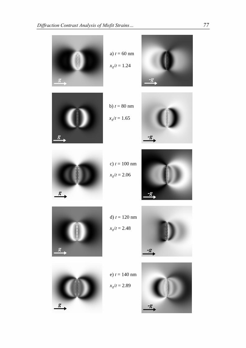
Diffraction Contrast Analysis of Misfit Strains… 77
e) t = 140 nm
ξg/t = 2.89
b) t = 80 nm
ξg/t = 1.65
c) t = 100 nm
ξg/t = 2.06
d) t = 120 nm
ξg/t = 2.48
a) t = 60 nm
ξg/t = 1.24
g
g
g
g
g
-g
-g
-g
-g
-g

78 Chapter 4
Fig. 4. Influence of specimen thickness on BF (left column) and (200)α-Fe centered DF
images (right column) of a misfitting VN particle of radius R = 7.5 nm and Burgers
vector b = 0.35 nm in the middle of an α-Fe foil. Thickness t relative to ξg, t ξg has
been indicated. See also Fig. 3.
10
8
6
4
2
0
par
ticle
lobe
dis
tanc
e (n
m)
151050R (nm)
Fig. 5. Influence of the particle radius R on the particle-lobe distances in BF and
(200)α-Fe centered DF images of a misfitting VN particle with Burgers vector b = 0.35
nm located in the middle of an 80 nm thick α-Fe foil.
2.2.2.4 Particle position
The influence of the vertical position (depth beneath the foil surface) of a particle in
the foil is shown in Fig. 7. The parameter ∆h indicates the vertical position with
respect to the middle of the foil (∆h = 0). The particle-lobe distances of the bright
lobes in BF and the dark lobes in centered DF are practically independent of ∆h,
although the full BF and centered DF images indicate a clear dependence on ∆h; only
if ∆h = 0 the full BF image is symmetric. For ∆h < 0, the same kind of results as for
∆h > 0 are obtained but the results of the BF left-hand lobe and the BF right-hand lobe
would have to be interchanged; the centered DF images are not dependent on the
direction of the particle shift (sign of ∆h).
It is concluded, when comparing full images of simulations and experiments
that as long as the experimental image in BF of the particle concerned is symmetric it
is justified in the simulation to assume that the particle is located in the middle of the
d lDF
drDF
d BF

Diffraction Contrast Analysis of Misfit Strains… 79
foil; for an analysis based on dBF and dDF only, small deviations of the location/depth
of the particle from the middle of the foil are irrelevant.
10
8
6
4
2
0
par
ticle
lobe
dis
tanc
e (n
m)
0.60.50.40.30.20.10.0b (nm)
Fig. 6. Influence of the particle Burgers vector b on the particle-lobe distances in BF
and (200)α-Fe centered DF images of a misfitting VN particle of radius R = 7.5 nm
located in the middle of an 80 nm thick α-Fe foil.
2.2.2.5 Neighbouring particle; overlapping strain fields
Consider a two-particle system with one particle located at (0,0,0) and the other one at
(L,0,0). The particle discs of equal particle radius, R = 7.5 nm, and particle Burgers
vector, b = 0.35 nm are parallel and located in the middle of a 80 nm thick foil. The
change of the image width for a change of the interparticle distance L from 10 nm to
150 nm is shown in Fig. 8. Obviously, for small L distinct effects on dBF and dDF
occur. Note that drBF is affected more than d l
BF since the right lobe is located closer
to the neighbouring particle than the left lobe. A similar statement holds for the
corresponding DF lobes. For L > 30 nm, i.e. L larger than about 1.5 times the particle
diameter, the influence of the neighbouring particle has become negligible and the
particle lobe distances are equal to those of a single misfitting particle of equal radius
and particle Burgers vector (cf. Fig. 7 at ∆h = 0).
Thus, comparing images simulated on the basis of a single particle model with
experimental contrast images of systems containing a high number density of
misfitting particles, in the experimental images particles should be selected that (i) are
d lDF
drDF
d BF

80 Chapter 4
10
8
6
4
2
0
par
ticle
lobe
dis
tanc
e (n
m)
1086420∆h (nm)
Fig. 7. Influence of the particle location on the particle-lobe distances in BF and(200)α-Fe centered DF images of a misfitting VN particle of radius R = 7.5 nm andBurgers vector b = 0.35 nm located in an 80 nm thick α-Fe foil. The particle isdisplaced upwards against the direction of electron motion by an amount ∆h (nm);∆h = 0 corresponds to the middle of the foil.
10
8
6
4
2
0
part
icle
lobe
dis
tanc
e (n
m)
1501251007550250L (nm)
Fig. 8. Influence of the distance L of a second particle (disc) located at (L,0,0) on theparticle-lobe distances in BF and (200)α-Fe centered DF images of a misfitting VNparticle at (0,0,0). The particle radius, R = 7.5 nm, and the Burgers vector, b = 0.35nm, of both particles are equal. The α-Fe foil is 80 nm thick.
d lDF
drBFdr
DF
d lBF
drDF
d lDFdr
BF
d lBF

Diffraction Contrast Analysis of Misfit Strains… 81
located at about 1.5, or more, times the particle diameter away from neighbouring
particles, and (ii) additionaly, exhibit symmetric contrast lobes in BF. The latter
criterion means that, additionaly, ∆h = 0. When the (projected) interparticle distance is
smaller, the influence of neighbouring particles can still be negligible if these particles
are situated at another height in the foil. Also for this case it holds that occurrence of a
symmetrical BF image of a single particle can be considered in general as indicative of
negligible influence of strain field overlap with neighbouring particles.
If the second particle at (L,0,0) is oriented perpendicularly with respect to the
first one at (0,0,0) (while remaining perpendicular to the foil surfaces), then the
displacements in the matrix caused by the second particle are directed perpendicularly
with respect to the displacements in the matrix from the first particle and also with
respect to the diffraction vector employed and therefore the effect of such a second
particle is negligible (cf. Eq. 1).
3. Specimen preparation
An α-Fe-2.2 at.% V solid solution was made through arc melting of 99.998 wt.% pure
α-Fe and 99.999 wt.% pure V in the correct ratio and subsequent annealing for 5 days
at 1225 ºC in an Ar-filled quartz ampul. The alloy composition was checked with
Electron Prope Micro Analysis: 0.4 at. % V is present as VO that developed during
the alloy production. In all further production steps the amount of VO remained
constant and therefore 1.8 at.% V is considered to be present initially in solid solution
and as VN after completed nitriding (see below).
A series of rolling and recrystallisation steps was applied to produce elongated
sheets of 200 µm thickness with crystallite sizes (optical microscopy) between 10 µm
and 60 µm. Small rectangular parts of size 1 cm × 2 cm cut from the sheet were
polished and thinned to about 100 µm thickness using Kawamura’s reagent [15].
Next, these pieces, suspended with a thin Ni wire, were through nitrided in a vertical
quartz tube furnace at 793 K, 853 K or 913 K for 25 hours. A gas mixture consisting
of 99 vol.% H2 (99.95 % purity) and 1 vol.% NH3 (99.90 % purity) was used, yielding
a constant nitriding potential of 0.0102 atm-1/2 during the time of nitriding [16].
Micro-Vickers hardness measurements at cross sections of the nitrided specimens
confirmed that through nitriding had occurred.
X-ray diffraction analysis of the nitrided specimens was performed on a
Siemens 500 B diffractometer equipped with Cu-Kα radiation and a graphite
monochromator in the diffracted beam to select Cu-Kα radiation. The specimens were
attached magnetically onto a Si- ⟨ ⟩510 single crystal substrate. The diffracted
intensities in the diffraction angle range of 20 -160 °2θ were recorded applying a 0.05

82 Chapter 4
º2θ stepsize and a 28 (s) counting time per step (yielding 15000 to 25000 counts at
{110} peak maximum depending on the specimen). During the measurement the
specimens were rotated about the specimen's surface normal.
From the nitrided material small circular discs of 3 mm diameter were drilled
that were polished with diamond paste (successively 3, 1 and 0.25 µm) to a thickness
of 20 µm. Subsequently, the specimens were jet-electrolytically polished in an acid
electrolyt (90 vol.% acetic acid, 10 vol.% perchloric acid) until perforation.
Transmission Electron Microscopy (TEM) was performed in a Philips CM30T
microscope operating at 150 kV. The low voltage of 150 kV (300kV is maximually
possible on the CM30T) was chosen to reduce the intensity of other than indicated
reflections in the systematic row …,-g, 0, g, 2g, …, as a low acceleration voltage
corresponds to a relatively large electron wavelength and a correspondingly relatively
small radius of Ewald's sphere. Selected Area Diffraction Patterns (SADP) as well as
BF's and centered DF's employing a (200)α-Fe reflection were recorded. At the SADP's
spots were observed at the location of the (forbidden) (100)α-Fe spots, which originated
most likely from the presence of Fe3O4 at the foil surface as grown after foil
preparation; see for a more elaborate discussion Ref. [17].
High Resolution Election Microscopy (HREM) images from the thin parts of
the foil were taken at 300 kV with the electron beam direction a few degrees away
from the [001]α-Fe zone axis, in such a way that a (110)α-Fe reflection was precisely in
the Bragg orientation. The objective aperture included the first-order reflections and
the transmitted beam.
All images and SADP's were recorded on photo negatives; for further
interpretation these were scanned using a commercially available scanning device
employing 600 dots per inch (dpi).
The thickness of the specimen foil was measured locally with the
contamination-spot separation method [18]. To this end, the vacuum of the
microscope was deteriorated deliberately by removing the cold trap, such that
contamination spots could be formed on both sides of the foil. The separation of the
spots was measured in projection for a series of different foil tilts leading to accurate
determination of the foil thickness at the location of the contamination spots.

Diffraction Contrast Analysis of Misfit Strains… 83
4. Fitting calculated diffraction contrast images to experimentaldiffraction contrast images of VN in αα-Fe
4.1 Selection of experimental diffraction contrast images of misfitting particles
An overview of the distribution of VN particles in the α-Fe-matrix and the strain
contrast caused by their displacement fields in the α-Fe-matrix is shown in the BF and
the (200)α-Fe centered DF images shown in Figs. 9a and 9b for a specimen nitrided at
913 K. The specimen is oriented with the electron beam almost perpendicular to the
specimen foil surface and ~ 2 ° out of the [001]-direction of the parent α-Fe-lattice
and g = (200)α-Fe. This arrangement of the specimen is used throughout this work. The
corresponding selected area diffraction pattern is given in Fig. 9c. For the specimens
nitrided at 793 K and 853 K the contrast changes in the images were much less
distinct; see also discussion in Section 5.
The diffraction pattern of the 913 K specimen shows two very strong spots, the
transmitted beam and the (200)α-Fe-diffraction spot, and two less strong spots, the
(400)α-Fe and (200)α-Fe diffraction spot. Streaks in the [100]α-Fe direction can be found
through the location of the {200}VN diffraction positions indicated by arrows in Fig.
9c. The elongated shape of these spots is caused by the small thickness of the disc-
shaped VN particles [19, 20] lying on (100)α-Fe lattice planes: measurement of the full
width at half maximum of both indicated {200}VN spots, in a way as usually carried
out in XRD [21], leads to an apparent VN particle thickness of 1.4 nm. Also VN
particles on other {100}α-Fe lattice planes (i.e. (010)α-Fe and (001)α-Fe) are present, but
these are not visible in the BF and the centered DF images since the corresponding
disc normals and the main matrix-lattice displacements are perpendicular to the
operating diffraction vector(s) (see also Section 2.2.2.5). Therefore, given a statistical
distribution of the VN particles over the three habit planes of type {100}α-Fe, only one
third of the total number of VN particles with their contrast lobes is visible in Figs. 9a
and 9b.
From the BF and centered DF images it is clear that the number density of VN
particles is very large. On the basis of the assumptions made in the model for the
image simulations (Section 2.1) and the calculated results (Section 2.2), in the
experimental images particles have been selected only when the following
requirements are met. (i) The particle should have close-to-symmetrical lobes in BF.
(ii) The particle should lie in the bright bend contour in the centered DF of g = (200)α-
Fe that corresponds to an exact realisation of the Bragg conditions. A possible
deviation from the Bragg position could not be assessed from analysis of Kikuchi

84 Chapter 4
(a) BF (b) centered DF
(c)
Fig. 9. BF image (a) and (200)α-Fe centered DF image (b) of Fe-2 at. % V specimen
nitrided for 25 hours at 913 K at nitriding potential of 0.0102 atm-1/2. Small VN
particles are visible surrounded by contrast lobes. The corresponding diffraction
pattern (c), with an orientation that is compatible with Figs. 9a and b, shows the
direct beam and the (200)α-Fe, (400)α-Fe and (2 00)a-Fe diffraction spots. Some iron
oxide reflections from a thin oxide layer on the surface are visible, see also Section 3.
Furthermore, {200}VN streaks in the [110]α-Fe-direction are visible as indicated by the
arrows. The specimen is oriented with the electron beam almost perpendicular to the
specimen foil surface and ~ 2 ° out of the [001]-direction of the parent α-Fe-lattice
and g = (200).
g -g
(200)α-Fe
_
particle I
(200)α-Fe
particle I
(400)α-Fe
50 nm 50 nm
(002)VN
(002)VN
_

Diffraction Contrast Analysis of Misfit Strains… 85
lines, since these could not be observed, possibly due to the straining of the matrix by
the large number of misfitting VN precipitates.
In this way three particles were selected, in the case corresponding to Fig. 9, of
which the contrast images are shown in BF and corresponding centered DF in Figs.
10-12. The average intensity distributions along a line perpendicular to the particles
and going through the centre of the particles are displayed in Fig. 13a for the BF
images and in Fig. 13b for the centered DF ones. The distributions have been averaged
over some distance (2.5 nm in total) perpendicular to this line to cancel out intensity
fluctuations caused by noise.
(BF) (centered DF)
Fig. 10. BF and (200)α-Fe centered DF image of selected VN particle I.
(BF) (centered DF)
Fig. 11. BF and (200)α-Fe centered DF image of selected VN particle II.

86 Chapter 4
(BF) (centered DF)
Fig. 12. BF and (200)α-Fe centered DF image of selected VN particle III.
Table 1: Particle-lobe distances in BF (drBF and d l
BF ; see Fig. 2) and corresponding
(200)α-Fe centered DF (drDF and d l
DF ; see Fig. 2) images with estimates of errors for
three selected particles of an Fe-2 at.% V alloy nitrided at 913 K. Particle radii, R,
are measured from the ends of the corresponding contrast lobes in BF and DF and
averaged.
particle d lBF dr
BF d lDF dr
DF R
(nm) (nm) (nm) (nm) (nm)
I 5.7 ± 0.2 6.3 ± 0.2 5.3 ± 0.2 5.3 ± 0.2 9.0 ± 0.2
II 4.1 ± 0.2 4.1 ± 0.2 4.5 ± 0.2 3.6 ± 0.2 5.3 ± 0.2
III 5.3 ± 0.4 4.9 ± 0.2 4.5 ± 0.3 4.5 ± 0.2 7.5 ± 0.2
The distances from the maximum intensity in each bright lobe in BF to the
particle, dBF, and from the minimum intensity in each dark lobe in centered DF, dDF,
along with an estimate of the measurement errors, are presented in Table 1. Note that
in case of particle I and particle III drDF ≈d l
DF , whereas in case of particle II
drDF ≠ d l
DF . For each particle also the particle radius is given as an average from the
measured distances between the ends of the contrast lobes above and below the
particle in BF and in centered DF. This distance does not deviate much from the
length of the dark line(s) of contrast in the images at the location of the particle
(visible particles are perpendicular to the foil).

Diffraction Contrast Analysis of Misfit Strains… 87
(a)
-10 -5 0 5 10
particle I
particle III particle II
Int
ensi
ty (
a.u.
)
(nm)
(b)
-10 -5 0 5 10
particle III
particle I
particle II
Int
ensi
ty (
a.u.
)
(nm)
Fig. 13. Normalised intensity distributions in BF (a) and (200)α-Fe centered DF (b)
obtained along the line through the centre of the selected particles I, II and III (cf.
Figs. 10, 11 and 12) and normalised with respect to the maximum and minimum
intensity within the range displayed.
4.2 Fitting of particle Burgers vector and foil thickness
The calculated images were fitted to the experimental ones by varying the values of t
and b; the value of R was set equal to the experimentally measured value (see Table
1). The fitting procedure ran as follows. (i) For wide ranges of values for the particle
Burgers vector b (0.2 nm to 0.5 nm in steps of 0.025 nm) and the specimen foil
thickness t (50 nm to 135 nm in steps of 2.5 nm) the intensity distribution was
calculated in BF and centered DF along the line perpendicular to the disc and going
through the centre of the disc and, subsequently, the values for the image widths d BF ,
d lDF and dr
DF were determined for each intensity distribution. (ii) Then, contour lines
of constant image width in (t,b) space were constructed for the experimental values of
d BF , d lDF , dr
DF . (iii) The intersection of the contour lines for d BF , d lDF and
drDF determined the t and b values for the particle concerned. (iv) Finally, full images

88 Chapter 4
were calculated for this combination of t and b values and were compared with the
experimental images. Only if sufficiently comparable images were obtained, the
corresponding values of t and b were accepted.
0.5
0.4
0.3
0.2
b (nm)
1251007550t (nm)
Fig. 14. Contour diagram for particle I showing contour plots of the three
experimentally measured particle-lobe distances, dBF (5.7 ± 0.2 nm), dDFl (5.3 ± 0.2
nm) and dDFr (5.3 ± 0.2 nm) as a function of the Burgers vector, b, and specimen
thickness, t, for a simulated VN particle with size R = 9.0 nm. For each particle-lobe
distance three lines are drawn: a centre line, corresponding to the mean value of the
particle-lobe distance, and two outer lines on either side of the centre line
corresponding to the mean value plus or minus the respective error indicated above.
The contour diagram for particle I with R = 9.0 nm, shown in Fig. 14, indicates
several regions of intersection for the contour lines of constant image width, i.e. (t,b)
combinations with which values for the particle-lobe distances equal to the
experimental ones are observed both in BF and centered DF: (i) a narrow band of
overlap between (t,b) = (50 nm, 0.425 nm) and (t,b) = (75 nm, 0.325 nm), (ii) at (t,b) =
(102.5 ± 0.5 nm, 0.42 ± 0.02 nm) and (iii) at (t,b) = (120 ± 0.5 nm, 0.34 ± 0.02 nm).
Note that the discontinuities in Fig. 14 for the contrast lines are related to the
discontinuities for the particle lobe distance as a function of t in Fig. 3.
Thus, on the basis of this contour diagram a unique choice of (t,b) cannot be
made. Therefore, a number of full BF and DF images with (t,b) combinations
corresponding to the above indicated regions of intersection were computed and
drDF
drDFd l
DF d BF
d lDF
d BF

Diffraction Contrast Analysis of Misfit Strains… 89
compared with the experimental ones. Representative results are shown in Fig. 15 for
a relatively thin foil (with (t,b) = (75.0 nm, 0.355 nm)), and a relatively thick foil
(with (t,b) = (121.2 nm, 0.342 nm)). Both simulated BF images resemble the
experimental image very well8. However, distinction can be made on the basis of the
centered DF images. The left-hand centered DF lobe for the case of the thick foil (Fig.
15b) does not appear as a curved contrast lobe as observed in the experimental image;
it merely shows a wide, diffuse zone without much contrast9. It is concluded that the
simulation for the case of the thin foil (Fig. 15a) is closer to reality. From a series of
simulations for a range of (t,b) values for the thin foil case, the following estimates
were eventually obtained for the foil thickness and the particle Burgers vector of
particle I: (t,b) = (73 ± 3 nm, 0.34 ± 0.02 nm). The value thus obtained for the foil
thickness agrees well with the value directly measured according to the contamination
spot method at the same location (cf. Section 3): tc = 80 ± 5 nm.
The contour diagrams for particle II and III with R = 5.3 nm and R = 7.5 nm,
respectively, are presented in Figs. 16 and 18. The same treatment as for particle I has
been applied to particles II and III. It was obtained for the foil thickness and the
particle Burgers vector of particle II, that (t,b) = (61 ± 3 nm, 0.45 ± 0.02 nm) and of
particle III, that (t,b) = (70 ± 3 nm, 0.35 ± 0.02 nm). Representative simulation results
for both particles can be compared with the respective experimental images in Fig. 17
for particle II and in Fig. 19 for particle III. The values thus obtained for the foil
thickness agree well with the values directly measured according to the contamination
spot method at the same locations: in case of particle II, tc = 62 ± 10 nm and in case of
particle III, tc = 67 ± 10 nm. All results of the fitting procedure have been collected in
Table 2.
8 Note, that the comparison of an experimental image with a calculated image is hindered by thedifferent grey scales of both images. Therefore, the exact intensities at a certain point in both imagescannot be compared on an absolute basis too strictly. Instead, characteristics of both images that are to alarge extent independent of the grey scales used can be compared, such as the extent and the shape ofthe bright and dark lobes.
9 Compare also with Figs. 4b and 4d, which display BF and centered DF images for similar thicknessand Burgers vector values, albeit for a somewhat larger particle.

90 Chapter 4
(a) (BF) (centered DF)
Fig. 15a. Comparison of experimental (lower part) and simulated (upper part) BF
image and (200)α-Fe centered DF image of particle I. Simulation was carried out for a
particle of radius R = 9.0 nm and Burgers vector b = 0.332 nm located in the middle
of a 75.0 nm thick foil.
(b) (BF) (centered DF)
Fig. 15b. Comparison of experimental (lower part) and simulated (upper part) BF
image and (200)α-Fe centered DF image of particle I. Simulation was carried out for a
particle of radius R = 9.0 nm and Burgers vector b = 0.342 nm located in the middle
of a 124.2 nm thick foil.

Diffraction Contrast Analysis of Misfit Strains… 91
b (nm)
1251007550 t (nm)
0.4
0.5
0.3
0.2
Fig. 16. Contour diagram for particle II showing contour plots of the three
experimentally measured particle-lobe distances, dBF (4.1 ± 0.2 nm), dDFl (4.5 ± 0.2
nm) and dDFr (3.6 ± 0.2 nm) as a function of the Burgers vector, b, and specimen
thickness, t, for a simulated VN particle with radius R = 5.3 nm. See also caption of
Fig. 14.
(BF) (centered DF)
Fig. 17. Comparison of experimental (lower part) and simulated (upper part) BF
image and (200)α-Fe centered DF image of particle II. Simulation was carried out for
a particle of size R = 5.3 nm and Burgers vector b = 0.45 nm located in the middle of
a 62.0 nm thick foil.
d lDF
drDF
d BF
drDF
d BF
d lDF

92 Chapter 4
b (nm)
1251007550t (nm)
0.5
0.4
0.3
0.2
Fig. 18. Contour diagram for particle III for the three experimentally measured
particle-lobe distances, d BF (4.9 ± 0.2 nm), d lDF (4.5 ± 0.2 nm) and dr
DF (4.5 ± 0.2 nm)
as a function of the Burgers vector b and specimen thickness t for a simulated VN
particle with radius R = 7.5 nm. See also caption of Fig. 14.
(BF) (centered DF)
Fig. 19. Comparison of experimental (lower part) and simulated (upper part) BF
image and (200)α-Fe centered DF image of particle III. Simulation was carried out for
a particle of size R = 7.5 nm and Burgers vector b = 0.35 nm located in the middle of
a 70.0 nm thick foil.
d BF
drDF
d lDF
d BF
d lDF
drDF

Diffraction Contrast Analysis of Misfit Strains… 93
Table 2: Burgers vector-length b and foil thickness t determined with the fitting
procedure for three selected particles of a nitrided Fe-2 at.% V alloy. The
specimen/foil thicknesses were also measured locally using the contamination-spot
separation method yielding tcont (see Section 3). R denotes particle radius.
Particle R b t tcont
(nm) (nm) (nm) (nm)
I 9.0 ± 0.2 0.34 ± 0.02 73 ± 3 80 ± 5
II 5.3 ± 0.2 0.45 ± 0.02 61 ± 3 62 ± 10
III 7.5 ± 0.2 0.35 ± 0.02 70 ± 3 67 ± 10
5. Additional results and discussion
5.1 Particle size and visibility of strain contrast
Using (200)α-Fe DF images of two different foils prepared from the same specimen
nitrided at 913 K, the size distribution of the VN particles was determined; the
average VN disc diameter is 13.1 nm, with a standard deviation of 7.6 nm, see Fig. 20.
The sizes of the particles investigated detailedly in Section 4 have been indicated. It is
concluded that the selected particles are representative for the system investigated.
Similarly the size distribution of the VN particles of specimen nitrided at 853
K was determined. In this case the average VN disc diameter is 5.1 nm, with a
standard deviation of 3.6 nm. Specimens nitrided at 793 K contain even smaller VN
particles since they could not be made visible in TEM and diffraction contrast lobes
could not be detected. This is consistent with the results from the simulations: for
particle radii smaller than about 2.5 nm (in a 80 nm thick sample and with a 0.35 nm
long Burgers vector) no contrast lobes in the matrix become distinct (see Fig. 5). Even
upon nitriding at 853 K contrast lobes can only rarely be observed, although particles
with a diameter larger than 5 nm then occur. This may at least partly be ascribed to
overlap of displacement fields of neighbouring VN particles. Note that, at constant V
content, the number of VN particles per unit of volume is relatively large if the
average size of the particles is relatively small.
5.2 Platelet thickness
The expected orientation relationship for a VN particle/disc in the α-Fe matrix is the
so-called Bain orientation relationship [19, 20, 22]

94 Chapter 4
0.20
0.15
0.10
0.05
0.00
P (R)
151050R (nm)
> 15
part
icle
II
part
icle
Ipart
icle
III
Fig. 20. Distribution of VN particle radii after nitriding an Fe-2 at.% V specimen for
25 hours at 913 K at a nitriding potential of 0.0102 atm-1/2. Particle radii are
measured using (200)α-Fe centered DF images of two different specimens. A total
amount of 360 particles was considered. Radii of the selected particles I, II and III
have been indicated.
{001}α-Fe//{001}VN; <100>α-Fe//<110>VN. (6)
The VN particles precipitate as platelets in α-Fe because the relative misfit in a
direction parallel to the platelet is small (2 %), whereas the relative misfit in the
direction perpendicular to the platelet is appreciable (44 %) [22]. The VN platelets
consist of a stack of a number of {001}VN lattice planes parallel with the {001}α-Fe
matrix lattice planes. If it is assumed that a coherent particle-matrix interface occurs
such that all misfit is accommodated elastically, it follows from Eq. (3b) that the
values of b obtained for particle I, II and III (see Table 2) correspond to a VN platelet
thickness of 1 to 1.4 nm, i.e. about 5 to 7 monolayers of {001}VN stacked on top of
each-other. This value of the thickness agrees very well with the value of 1.4 nm
derived from the length of the {200}VN streaks, as discussed in Section 4.1.
5.3 Occurrence of misfit dislocations; lattice plane imaging
For platelets of relatively large thickness it is conceivable that the platelet/matrix
misfit can no longer be accommodated fully elastically. If the misfit exceeds a critical
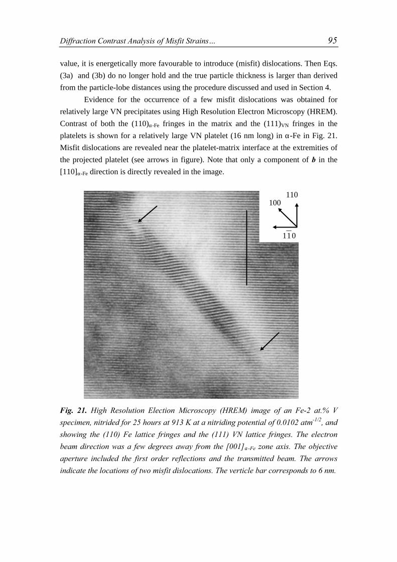
Diffraction Contrast Analysis of Misfit Strains… 95
value, it is energetically more favourable to introduce (misfit) dislocations. Then Eqs.
(3a) and (3b) do no longer hold and the true particle thickness is larger than derived
from the particle-lobe distances using the procedure discussed and used in Section 4.
Evidence for the occurrence of a few misfit dislocations was obtained for
relatively large VN precipitates using High Resolution Electron Microscopy (HREM).
Contrast of both the (110)α-Fe fringes in the matrix and the (111)VN fringes in the
platelets is shown for a relatively large VN platelet (16 nm long) in α-Fe in Fig. 21.
Misfit dislocations are revealed near the platelet-matrix interface at the extremities of
the projected platelet (see arrows in figure). Note that only a component of b in the
[110]α-Fe direction is directly revealed in the image.
Fig. 21. High Resolution Election Microscopy (HREM) image of an Fe-2 at.% V
specimen, nitrided for 25 hours at 913 K at a nitriding potential of 0.0102 atm-1/2, and
showing the (110) Fe lattice fringes and the (111) VN lattice fringes. The electron
beam direction was a few degrees away from the [001]α-Fe zone axis. The objective
aperture included the first order reflections and the transmitted beam. The arrows
indicate the locations of two misfit dislocations. The verticle bar corresponds to 6 nm.
110100
110

96 Chapter 4
5.4 X-ray diffraction line-shift and -broadening
The {222}α-Fe diffraction line profiles of an unnitrided specimen and of specimens
nitrided at 793 K, 853 K and 913 K are presented in Fig. 22 (note the logarithmic
intensity scale). Upon nitriding a strong asymmetrical line broadening takes place: the
peak maximum shifts appreciably from the peak position of the line profile of the
unnitrided specimen and asymmetrical, distinct tails appear. The tail at the high angle
side is more pronounced that the one at the low angle side. This type of line
broadening is typical for the case of small coherent inclusions in a matrix with elastic
accommodation of the misfit [23-27]. Only in case of the specimen nitrided at 913 K a
separate { }200 VNXRD reflection could be observed (near 43.7 º2θ), in accordance with
the presence of elongated { }200 VNTEM spots in the selected area diffraction pattern of
Fig. 9c.
The shape and the width of the measured line profiles are interpreted now
considering their Fourier transforms. In order to remove the broadening due to the
wavelength distribution and the instrumental aberrations the {533} line profile of a
150145140135130125
2θ
log(
Inte
nsity
) (a
.u.)
793 K
913 K
853 K
not nitrided
{222}α-Fe
Fig. 22a. X-Ray diffraction line profiles recorded for the {222}α-Fe reflection of
different Fe-2 at.% V samples nitrided for 25 hours at 793 K, 853 K or 913 K at a
nitriding potential of 0.0102 atm-1/2 and of a not-nitrided reference sample. Vertical
bars indicate the centroid positions of the respective line profiles; see also Table 3.
º2θ

Diffraction Contrast Analysis of Misfit Strains… 97
1.0
0.8
0.6
0.4
0.2
0.0
|F(L)|
100806040200L (nm)
913 K
853 K
793 K
Fig. 22b. Modulus of the Fourier transforms of the only structurally broadened
{222}α-Fe reflections of different Fe-2 at.% V samples, nitrided for 25 hours at 793 K,
853 K or 913 K at a nitriding potential of 0.0102 atm-1/2.
specially made strain free Si-powder sample [28], with a peak position close to the
peak position of the {222}α-Fe line profile, was used to deconvolute the line profiles
measured [4]. The results, in terms of the Fourier transform, F(L), with L as a
correlation distance, of the only structurally broadened line profiles, are presented in
Fig. 22b. In case of the Fourier transform of the specimen nitrided at 793 K F(L)
decreases for short correlation lengths (0 < L < 10 nm to 15 nm) to a more or less
constant value10. This more or less constant level of the Fourier transform is
equivalent to the presence of a sharp Bragg-like peak in the intensity distribution (cf.
Fig. 22a) [31]. This observation is interpreted such that in the specimen nitrided at 793
K (and possibly also in the one nitrided at 853 K) apparently, the lattice distortions
brought about by the misfitting particles do not disturb the phase relation between
atoms at large correlation distances. In case of the specimen nitrided at 913 K such a
non-zero constant level for the Fourier transform of the line profile is not observed:
the phase relations between atoms separated by a distance L > 30 nm have become 10 The more or less periodic ripple observed for F(L) nitrided at 793 K at approximately L = 16, 48 and80 nm and the slight decrease upon increasing L for the plateau level of F(L) for the specimens nitridedat 793 K and 853 K can be ascribed fully to minor shape differences of the instrumental {533}Si lineprofile and the {222}α-Fe line profile due to counting statistics and different measurement conditions(step size and slit size) (see discussion in Refs. 29 and 30).

98 Chapter 4
totally uncorrelated. It has been suggested that this effect occurs for lengths of L
encompassing 2 to 3 interparticle distances [25]. Indeed, it follows from Figs. 9a and
9b in case of the specimen nitrided at 913 K that a distance of 30 nm includes
approximately 2 to 3 particles.
The centroid positions of the {222}α-Fe line profiles, measured for an
unnitrided specimen and specimens nitrided at 793 K, 853 K and 913 K, were
determined, see Fig. 22a and Table 3. The line profile centroids are shifted towards
the low angle side with respect to centroid of the unnitrided specimen; the centroid
shifts of the nitrided specimens increase for decreasing nitriding temperature. The
following causes for the line profile centroid shifts can be considered.
Table 3: Centroids of {222}α-Fe line profiles, 1 222dc{ } or 2θc, of an unnitrided
specimen and specimens nitrided at 793 K, 853 K or 913 K. The centroids were
calculated on a 1/d-scale.
Specimens unnitrided 793 K 853 K 913 K
1 222dc{ } (nm-1) 12.081 12.067 12.076 12.087
º2θc 137.28 136.96 137.18 137.44
Firstly, V depletion of the matrix due to precipitation of the substitutionally
dissolved V as VN induces a temperature independent centroid shift. Using Vegard's
law [32] and the lattice constant of V, aV = 0.30232 nm [12], a centroid shift upon
precipitation is determined towards the high angle side, which is not observed
implying that this effect does not dominate the occuring centroid shift.
Secondly, interstitially dissolved N in the matrix after precipitation leads to
centroid shifts that can be shown to be much smaller than the observed ones.
Thirdly, following a model described in Ref. [22], a positive hydrostatic strain
emerges upon precipitation of VN in the α-Fe matrix as a consequence of the elastic
accommodation of the precipitate/matrix misfit, which causes the centroid to shift
towards the low angle side, as observed. The model assumes the presence of (i)
misfitting VN platelets in a finite α-Fe-matrix and of (ii) extra (excess) N atoms
adsorbed (and located in octahedral interstices) at the interface of the VN precipitates
and the α-Fe-matrix. The extra N atoms effectively enlarge the misfit of the VN
precipitates with respect to the α-Fe-matrix. The amount of excess N adsorbed at the
platelett/matrix interface has been derived from mass measurements before and after
the nitriding; these amounts decreased for increasing nitriding temperatures [22]. Then
the centroid shift towards lower diffraction angles would decrease for increasing

Diffraction Contrast Analysis of Misfit Strains… 99
nitriding temperature, which agrees with the present experimental observation. A
quantitative assessment cannot be made as the matrix should diffract fully
independently from the VN particles, which, especially for the relatively low nitriding
temperatures, appears not to be the case (see above).
6. Conclusions
Diffraction contrast simulation model
- The strain field surrounding misfitting inclusions can be characterized quantitatively
comparing simulated and measured full diffraction-contrast Transmission Electron
Microscopy (TEM) images.
- The misfit, as indicated by a "particle Burgers vector", for disc shaped
inclusions/precipitates, can be determined unambiguously from the contrast lobes
widths ("image widths") as measured in both bright field and dark field.
- For determination of the particle Burgers vector diffraction-contrast image
simulations can be based on a system of a single particle in an infinite matrix, as the
inner parts of the contrast images are practically unaffected by the presence of
neighbouring particles.
Misfitting VN particles in α-Fe matrix
- Upon nitriding of an Fe-2 at.%V alloy small misfitting VN platelets are formed
along {001}α-Fe with {001}VN parallel to {001}α-Fe. The platelet/disc radius increases
with increasing nitriding temperature from a few nanometers after nitriding at 793 K
to 13 ± 7 nm after nitriding at 913 K. After nitriding at 913 K the platelet thickness
equals about 1 to 1.4 nm as indicated by both the diffraction strain contrast
(simulations) and the extent of the VN precipitate diffraction streaks. The misfit is
largely accommodated elastically; only a few misfit dislocations were observed in
High Resolution Electron Microscopy images for only the larger VN precipitates
- The observed diffraction contrast images after nitriding at 913 K could be simulated
well using the diffraction and strain models.
- On the basis of the contrast lobe widths in bright field and dark field combinations of
possible values for the "Burgers vector of the particle", b, and the thickness of the foil,
t, were obtained. Selection of the correct combination of b and t was possible by
comparing the full simulated and experimental diffraction-contrast images. The fitted
value of the local foil thickness agrees well with the value determined directly by the
contamination-spot method at the location of the precipitate.
100 Chapter 4
- The observed shifts and broadenings of the XRD profiles support the results
obtained using TEM.
Acknowledgements
This work has been part of the research program of the Foundation for Fundamental
Research on Matter (Stichting FOM), The Netherlands. The authors are indebted to
Ing. N. Geerlofs for the provision of the nitriding equipment, to Mr. T.R. de Kruijff
for assistance with the TEM specimen preparation, to Dr. K.G.F. Janssens for the
provision of the SIMCON-simulation program and finally to Dr. R. Delhez for
stimulating discussions.
Appendix Rearrangement of Howie-Whelan equations for a four beam case
Analogous to the procedure given in Ref. [7] for a two beam case, each amplitude
Φ g j of the (four) coupled differential equations of Eq. (1) is multiplied by an
additional phase factor such that the term ( )g g uj k− ⋅ arises only once in every
differential equation. This leaves the intensity of each beam at the bottom of the
specimen unaffected because any additional phase factor cancels out when the
amplitudes are multiplied by their complex conjugates, but the numerical integration
of Eq. (1) is accellerated greatly.
The new amplitude equations are written as
ddz
AΦΦ ΦΦ= (A. 1)
where ΦΦ is a column vector containing the real and imaginary parts of the opering
beams
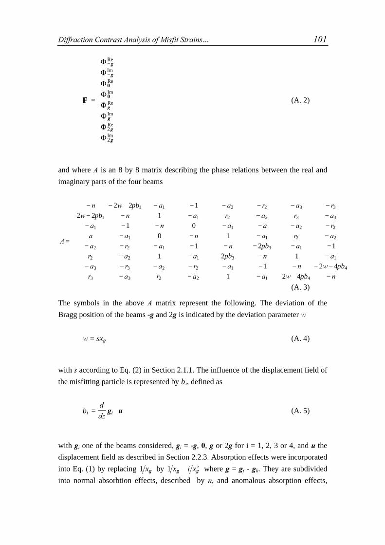
Diffraction Contrast Analysis of Misfit Strains… 101
ΦΦ =
−
−
ΦΦΦΦΦΦΦΦ
g
g
g
g
g
g
Re
Im
Re
Im
Re
Im
Re
Im
0
0
2
2
(A. 2)
and where A is an 8 by 8 matrix describing the phase relations between the real and
imaginary parts of the four beams
A
n w a a r a rw n a r a r a
a n a a a ra a n a r aa r a n a
r a a n aa r a r a n w
r
=
− − + − − − − − −− − − − −− − − − − − −
− − − −− − − − − − − −
− − − −− − − − − − − − −
2 2 12 2 1
1 00 1
1 2 11 2 1
1 2 4
1 1 2 2 3 3
1 1 2 2 3 3
1 1 2 2
1 1 2 2
2 2 1 3 1
2 2 1 3 1
3 3 2 2 1 4
3
πβπβ
πβπβ
πβ− − − + −
a r a a w n3 2 2 1 41 2 4πβ
(A. 3)
The symbols in the above A matrix represent the following. The deviation of the
Bragg position of the beams -g and 2g is indicated by the deviation parameter w
w s= ξg (A. 4)
with s according to Eq. (2) in Section 2.1.1. The influence of the displacement field of
the misfitting particle is represented by βi, defined as
βi iddz
= ⋅g u (A. 5)
with gi one of the beams considered, gi = -g, 0, g or 2g for i = 1, 2, 3 or 4, and u the
displacement field as described in Section 2.2.3. Absorption effects were incorporated
into Eq. (1) by replacing 1 ξg by 1 ξ ξg g+ ′i where g = gj - gk. They are subdivided
into normal absorbtion effects, described by n, and anomalous absorption effects,

102 Chapter 4
described by a1, a2 and a3. The ratios between the extinction distances used are given
by r1, r2 and r3:
n
a a a
r r r
g
g
g
g
g
g
g
g
g
g
g
g
g
=
= = =
= = = =
ξξ
ξξ
ξξ
ξξ
ξξ
ξξ
ξξ
0
1 22
33
1 22
23
1
'
' ' ', ,
, ,
(A. 6)
References
[1] G.E. Dieter, Mechanical Metallurgy, McGraw-Hill, Singapore, 1987.
[2] M.F. Ashby and L.M. Brown, Phil. Mag. 8 (1963), 1083.
[3] M.F. Ashby and L.M. Brown, Phil. Mag. 8, (1963), 1649.
[4] E.J. Mittemeijer, P. van Mourik, Th.H. de Keijser, Phil. Mag. A43 (5), (1981), 1157.
[5] J.G.M. van Berkum, R. Delhez, Th.H. de Keijser, E.J. Mittemeijer, P. van Mourik, Scripta
Metall. et Mater. 25, (1991), 2255.
[6] A. Howie, M.J. Whelan, Proc. Roy. Soc. A 263 (1961), 217.
[7] P.B. Hirsch, A. Howie, R.B. Nicholson, D.W. Pashley, Electron microscopy of thin
crystals, Butterworths, London, 1967.
[8] J.D. Eshelby, Proc. Roy. Soc. A 241 (1957) 376.
[9] K.G.F. Janssens, Localized strain characterization using electron diffraction contrast
imaging, Ph.D. thesis, KU Leuven, 1995.
[10] W.H. Press, S.A. Teukolsky, W.T. Vetterling, B.P. Flannery, Numerical Recipes in
Fortran, Cambridge University Press, 1986.
[11] P. Stadelmann, Ecole Polytechnique Fédérale de Lausanne, EMS OnLine,
"http://cimesg1.epfle.ch/EMS/", 05-09-1997.
[12] Powder Diffraction File, International Centre for Diffraction Data, Swarthmore, PA,
1988.
[13] H. Hashimoto, A. Howie, M.J. Whelan, Phil. Mag. 5 (1960), 967.
[14] H. Hashimoto, A. Howie, M.J. Whelan, Proc. Roy. Soc. A 269 (1962) 80.
[15] K. Kawamura, J.Japan Inst. Metals 24 (1960), 710.
[16] E.J. Mittemeijer, J.T. Slycke, Härterei Tech. Mit. 50 (1995), 2.
[17] M.H. Biglari, C.M. Brakman, E.J. Mittemeijer, Phil. Mag. A 72 (5) (1995), 1281.
[18] D.B. Williams, C.B. Carter, Transmission Electron Microscopy, a Textbook for
Materials Science, Plenum Press, New York, 1996.
[19] M. Pope, P. Grieveson, K.H. Jack, Scan. J. of Metallurgy 2, (1973), 29.
[20] M.M. Yang , A.D. Krawitz, Metall. Trans. A. 15A (1984), 1545.
[21] B.E. Warren, X-Ray Diffraction, Reading, Massachusetts: Addison-Wesley, 1969.

Diffraction Contrast Analysis of Misfit Strains… 103
[22] M.A.J. Somers, R.M. Lankreijer, E.J. Mittemeijer, Phil. Mag. A 59, (1989), 353.
[23] M.A. Krivoglaz, X-Ray and Neutron Diffraction in Nonideal Crystals, Springer, Berlin,
1996.
[24] C.R. Houska, Acta Cryst. A49, (1993), 771.
[25] R. Kuzel, B. He, C.R. Houska, J. Mat. Sci. 32 (1997), 2451.
[26] T.C. Bor, R. Delhez, E.J. Mittemeijer, E. Van der Giessen, to be published (Chapters 2
and 3).
[27] L. Velterop, R. Delhez, Th.H. de Keijser, E.J. Mittemeijer, to be published.
[28] J.G.M. van Berkum, G.J.M. Sprong, Th.H. de Keijser, R. Delhez, E.J. Sonneveld,
Powder Diffraction 10 (2), (1991), 129.
[29] T.C. Bor, M.C. Huisman, R. Delhez, E.J. Mittemeijer, Mat. Sci. For. 278-281 (1998),
145.
[30] T.C. Bor, M.C. Huisman, J.-D. Kamminga, E.J. Mittemeijer, E. Van der Giessen, to be
published (Chapter 6)
[31] R.N. Bracewell, The Fourier Transform and its Applications, McGraw-Hill, Tokyo,
1978.
[32] J.W. Christian, The Theory of Transformations in Metals and Alloys, Pergamon,
Oxford, 1965.


Chapter 5
A Method to Determine the Volume Fractionof a Separate Component in a Diffracting Volume
T.C. Bor1, M.C. Huisman2, R. Delhez1 and E.J. Mittemeijer1, 3
1Laboratory of Materials Science, Delft University of Technology,
Rotterdamseweg 137, 2628 AL Delft, The Netherlands2Faculty of Sciences, Division of Physics and Astronomy,
vrije Universiteit Amsterdam
De Boelelaan 1081, 1081 HV Amsterdam, The Netherlands3Max Planck Institute for Metals Research,
Seestraße 92, 70174 Stuttgart, Germany
Abstract
An (X-ray) diffraction line-profile analysis method has been proposed to determine the
volume fraction of a component with a “homogeneous” microstructure that forms part of a
sample that is, overall, microstructurally non-homogeneous. The method is based on
deconvolution of a measured line profile of the sample to be analysed with a line profile
separately measured from material that is microstructurally identical to the homogeneous
component in the mixture. Consequences of counting statistical variations for the application
of the method have been analysed. The method has been applied to ball milled Mo powder to
determine the volume fraction of the undeformed powder present in the ball-milled powder.
1. Introduction
The analysis of X-ray diffraction (XRD) line broadening enables the determination of
quantities such as the “size” of and the “microstrain” within the crystallites contained
in the diffracting volume [1]. The results of an XRD measurement have to be
interpreted as a volume weighted average of these quantities over the diffracting
crystallites in the volume irradiated. Hence, straightforward interpretation of the
broadening of XRD line profiles measured from microstructurally non-homogeneous
materials is impossible. However, if one separate microstructurally homogeneous
component can be identified in this non-homogeneous diffracting volume, the volume
fraction of the homogeneous component and the line broadening due to only the

106 Chapter 5
remaining material in the diffracting volume can be determined. To this end a
deconvolution method is presented here. The effect of counting statistics is analysed
quantitatively, leading to a procedure for application of the method proposed.
The diffraction analysis of an initial stage of the deformation process of Mo
powder in a ball mill will be given as an example for the procedure proposed.
2. Theoretical basis
The result of an XRD measurement can be given in the form of a line profile: i.e. the
measured diffracted intensity I as a function of the diffraction angle 2θ or the length of
the diffraction vector. A measured line profile (h-profile) can be described as the
convolution of the structural line profile (f-profile) with the instrumental line profile
(g-profile). Convolution of two functions in real space is equivalent to the
multiplication of their respective Fourier transforms in Fourier (reciprocal) space [2].
The Discrete Fourier Transform (DFT) of a function h(t) given by N equidistant
sample values (t = 0, 1, 2, ..., (N-1)) is given by:
( ) ( ) ( )H n h t int Nt
N= ∑
=
−exp 2
0
1π , (1)
where n denotes the harmonic number, n = 0, 1, 2, ..., (N - 1), and N can be written as
p/∆t, with ∆t as the sampling distance in real space and p as the period of the function
in real space.
Consider the situation in which a separate component A can be identified in
the total diffracting volume composed of (homogeneous) component A and the rest of
the (inhomogeneous) diffracting volume, component B. According to the kinematical
diffraction theory the total intensity diffracted by a volume of material for a {HKL}
reflection, ItotHKL ( )2θ , is equal to the sum of the diffracted {HKL} intensities from the
individually (i.e. incoherently) diffracting crystallites. Hence, ItotHKL ( )2θ can be written
as the volume weighted sum of the intensity diffracted by crystallites belonging to
component A, I AHKL ( )2θ , and the intensity diffracted by crystallites belonging to
component B, IBHKL ( )2θ :
( ) ( ) ( ) ( )I I ItotHKL
AHKL
BHKL2 2 1 2θ α θ α θ= + − , (2)
where α denotes the volume fraction of diffracting crystallites of component A.

A Method to Determine the Volume Fraction of… 107
Using the additivity of DFT’s, it follows from Eq. (2):
( ) ( ) ( ) ( )H n H n H ntotHKL
AHKL
BHKL= + −α α1 , (3)
where H ntotHKL ( ) , H nA
HKL ( ) and H nBHKL ( ) are the DFT’s of the corresponding line
profiles, normalised such that H H HtotHKL
AHKL
BHKL( ) ( ) ( )0 0 0 1= = = .
Now, to determine α and IBHKL ( )2θ , it will be supposed that I A
HKL ( )2θ can be
recorded from a material that has a microstructure identical to that of component A in
the sample to be analysed. For this line profile, to be denoted by IsHKL ( )2θ , it thus
holds:
( ) ( )I IsHKL
AHKL2 2θ θ= and ( ) ( )H n H ns
HKLAHKL= . (4)
Deconvolution of ItotHKL ( )2θ with I s
HKL ( )2θ can be carried out according to:
( ) ( )( ) ( ) ( )
( )D n A n iB n
H n
H n
H n
H nHKL
DHKL
DHKL tot
HKL
sHKL
BHKL
AHKL
≡ + ≡ = + −( ) ( ) α α1 , (5)
with ( )DHKL 0 1= ; A nDHKL ( ) and B nD
HKL ( ) represent the real and the imaginary parts of
D nHKL ( ) .
Note that the line profile IsHKL ( )2θ , acting as a “g-profile” in the
deconvolution, need not have as little structural broadening as possible. If the line
profile resulting from the crystallites belonging to component A is less broad on a 2θaxis than the line profile resulting from the rest of the crystallites, i.e. component B,
then the second term at the right-hand side of Eq. (5) vanishes for sufficiently large n.
Then D nHKL ( ) becomes equal to α. Thereby not only the volume fraction α of
component A can be determined in principle, but subsequently H nBHKL ( ) (and
IBHKL ( )2θ ) can be obtained as well. Obviously, as in “normal” deconvolution
procedures (cf. Ref. 3), the accuracy in the values obtained for the desired parameters,
here α (and H nBHKL ( ) ), is strongly determined by counting statistical variations in the
values of H ntotHKL ( ) and H ns
HKL ( ) . This effect will be discussed in section 4.
3. Experimental
Mo powder (Alpha, 99.9 wt-% pure, almost spherical particles with diameter 1 - 7
µm) was ball milled in vacuum for 30 minutes in a low energy ball mill. This ball mill

108 Chapter 5
is an evacuated vibrating cylindrical vessel with a bottom plate of WC - whereupon
the Mo powder is deposited - and that contains a ferritic stainless steel ball. Scanning
Electron Microscopy analysis (see [4] for more experimental details and results) of
undeformed starting powder (further denoted Mo0) and deformed powder (further
denoted Mo30) suggested, from the shape of the powder particles, that the Mo30
powder consists of deformed (crushed) particles as well as undeformed particles
(Mo0).
To enable a study of the kinetics of the deformation process of Mo in the ball
mill it is imperative to determine the volume fraction of the remaining undeformed
component as function of ball milling parameters. To this end the procedure proposed
in section 2 was applied where the undeformed component is taken as component A.
Small volumes of the Mo0 powder and of the Mo30 powder were deposited onto
Si 510 -single crystal wafers to enable XRD-measurements [5]. These measurements
were performed on a Siemens F-ω diffractometer equipped with a curved graphite
monochromator in the diffracted beam. From both specimens the {110} reflections
were measured in the same way using Cu-Kα radiation within the 2θ-range 32.5 °2θto 51.0 °2θ using a 0.01 °2θ stepsize and a 2 (s) counting time. Each specimen was
measured five times consecutively to study the reproducibility of the measurements
and the influence of counting statistical errors.
4. Results and discussion
The as-measured line profiles corresponding to the {110}-reflections of both the Mo0
specimen and the Mo30 specimen are shown in Fig. 1. The line profiles have been
normalised by division by their integral intensities. Clearly, the {110} line profile of
the Mo30 powder is broader than that of the Mo0 powder (see in particular the lower
intensity maxima for the Mo30 powder).
A linear background determined by a least-squares fit through the first and last
5 % of the data points was subtracted from the line profiles measured. Identifying the
{110} profile of the Mo30 powder as I totHKL ( )2θ and the {110} profile of the Mo0
powder as I sHKL ( )2θ , Eq. (5) was applied. To avoid effects on A110(n) and B110(n) due
to non-coincidence of centroid and origin of the abcissa in real space, the modulus of
D110(n), |D110(n)|, is considered (Fig. 2a).
From Fig. 2a it follows that with increasing value of the harmonic number n,
|D110(n)| decreases from |D110(n)| = 1 to a more or less constant value of approximately
α = 0.76 for 150 < n < 220, indicating that the ball milled powder contains a certain
volume fraction of undeformed particles. For still higher values of n, |D110(n)| starts to
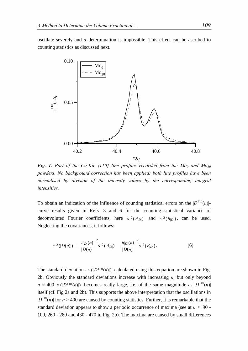
A Method to Determine the Volume Fraction of… 109
oscillate severely and α-determination is impossible. This effect can be ascribed to
counting statistics as discussed next.
0.10
0.05
0.00
I110 (º
2θ)
40.840.640.440.2
º2θ
Mo0
Mo30
Fig. 1. Part of the Cu-Kα {110} line profiles recorded from the Mo0 and Mo30
powders. No background correction has been applied; both line profiles have been
normalised by division of the intensity values by the corresponding integral
intensities.
To obtain an indication of the influence of counting statistical errors on the |D110(n)|-
curve results given in Refs. 3 and 6 for the counting statistical variance of
deconvoluted Fourier coefficients, here σ 2 ( )| |AD and σ 2 ( )| |B D , can be used.
Neglecting the covariances, it follows:
σ σ σ22
22
2(| ( )|)( )
| ( )|( )
( )
| ( )|( )| |
| || |
| |D nA n
D nA
B n
D nBD
DD
D=
+
. (6)
The standard deviations σ (| ( )|)D n110 calculated using this equation are shown in Fig.
2b. Obviously the standard deviations increase with increasing n, but only beyond
n ≈ 400 σ (| ( )|)D n110 becomes really large, i.e. of the same magnitude as |D110(n)|
itself (cf. Fig 2a and 2b). This supports the above interpretation that the oscillations in
|D110(n)| for n > 400 are caused by counting statistics. Further, it is remarkable that the
standard deviation appears to show a periodic occurrence of maxima (see at n ≈ 90 -
100, 260 - 280 and 430 - 470 in Fig. 2b). The maxima are caused by small differences

110 Chapter 5
between the ( )I A110 2θ component profile of the ( )I tot
110 2θ line profile, and the
separately measured ( )I s110 2θ profile, due to occurrence of counting statistical
variations in the intensity values. In the absence of counting statistics both profiles
would be equal, as implied by Eq. (4). The shape differences are most pronounced at
2θ locations where the intensities are large, i.e. at and around peak maxima.
Consequently the Kα1-Kα2 doublet nature reveals itself in the occurrences of periodic
maxima in σ (| ( )|)D n110 as will be shown below (see also Ref. 7).
1.0
0.9
0.8
0.7
0.6
0.5
|D11
0 (n)|
5004003002001000n
Fig. 2a. The modulus of D110(n) (cf. Eq. (5)) as obtained from the profiles shown in
Fig. 1.
0.001
0.01
0.1
1
10
σ110 (n
)
5004003002001000
n
Fig. 2b. The counting statistical variance of the modulus of the Fourier coefficients of
D110(n) shown in Fig. 2a (cf. Eq. (6)) (logarithmic ordinate!).
Suppose the Kα1-Kα2 doublet (of component A) consists of the sum of a
single peaked function, I(2θ), with its top at the origin of the 2θ-axis and a scaled

A Method to Determine the Volume Fraction of… 111
(R = 0.5) and displaced (∆ °2θ) version of the same function, RI(2θ - ∆), and thus
Iα α θ1 2 2/ ( ) = I(2θ) + RI(2θ - ∆). To illustrate the effects of counting statistical shape
differences a second doublet is constructed that is equal to the first doublet but in
addition a “delta” peak with area Ic is added at the top position of the Kα1-peak and
thus I I RI Icα αδ
αθ θ θ δ θ1 2 12 2 2 2/max( ) ( ) ( ) ( )= + − +∆ . If the Fourier transform of this
affected, second doublet is divided by the Fourier transform of the unaffected, first
doublet (similar to the procedure outlined in section 2 with Iα αδ θ1 2 2/ ( ) as I tot ( )2θ and
Iα α θ1 2 2/ ( ) as I s ( )2θ ) the result is:
D nI A n R n N B n R n N I
H n R n N Rc H H c( )
( )( cos( ) ( )( sin( )
| ( )| ( cos( ) )= +
+ + ++ +
12 1 2 2 2
1 2 2
2
2 2
π ππ
∆ ∆∆
, (7)
with H(n) as the Fourier transform of Iα α θ1 2 2/ ( ) and with ∆ expressed as a number of
steps; A nH ( ) and B nH ( ) represent the real and the imaginary parts of D(n). In the case
of a Lorentzian shape function for I(2θ), with maximum intensity I0 and full width at
half maximum 2w, Eq. (7) becomes approximately:
D nIwI
en N
c wn( )cos( )
≈ + ++
1
21
3 4
5 4 20
2
π ππ
∆. (8)
If a deconvolution procedure like the one described by Eq. (5) is performed, it follows
simply from Eq. (8) that the intensity aberration at the top of a Kα1 peak leads to
effects in Fourier space such that local error maxima occur at approximately
n N N= 2 3 2∆ ∆, , ... and local error minima at n N N= 0 2, , ,... ∆ ∆ . For the case
shown in Fig. 2 it holds that N = 1851 and ∆ = 10 and therefore the spacing between
the local maxima and between the local minima in Fig. 2b should be N/∆ ≈ 185,
which agrees well with the experimental observation reported above.
From the above analysis it follows that the value of α can best be determined
from |D110(n)| where n is sufficiently large and the estimated standard deviation show
a local minimum; i.e. within the range of Fourier numbers 160 < n < 190 (cf. Fig. 2).
The corresponding results of the proposed deconvolution method as obtained for five
consecutive measurements performed under similar conditions are given in Table 1.
Clearly good reproducibility has been achieved. The remaining small differences in
the α values are ascribed to the effect of counting statistics (for n ≈ 200 σ ≈ 0.02, cf.
Fig. 2b).
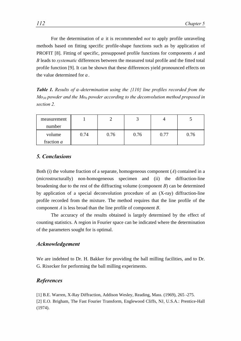
112 Chapter 5
For the determination of α it is recommended not to apply profile unraveling
methods based on fitting specific profile-shape functions such as by application of
PROFIT [8]. Fitting of specific, presupposed profile functions for components A and
B leads to systematic differences between the measured total profile and the fitted total
profile function [9]. It can be shown that these differences yield pronounced effects on
the value determined for α.
Table 1. Results of α-determination using the {110} line profiles recorded from the
Mo30 powder and the Mo0 powder according to the deconvolution method proposed in
section 2.
measurement
number
1 2 3 4 5
volume
fraction α0.74 0.76 0.76 0.77 0.76
5. Conclusions
Both (i) the volume fraction of a separate, homogeneous component (A) contained in a
(microstructurally) non-homogeneous specimen and (ii) the diffraction-line
broadening due to the rest of the diffracting volume (component B) can be determined
by application of a special deconvolution procedure of an (X-ray) diffraction-line
profile recorded from the mixture. The method requires that the line profile of the
component A is less broad than the line profile of component B.
The accuracy of the results obtained is largely determined by the effect of
counting statistics. A region in Fourier space can be indicated where the determination
of the parameters sought for is optimal.
Acknowledgement
We are indebted to Dr. H. Bakker for providing the ball milling facilities, and to Dr.
G. Rixecker for performing the ball milling experiments.
References
[1] B.E. Warren, X-Ray Diffraction, Addison Wesley, Reading, Mass. (1969), 265 -275.
[2] E.O. Brigham, The Fast Fourier Transform, Englewood Cliffs, NJ, U.S.A.: Prentice-Hall
(1974).

A Method to Determine the Volume Fraction of… 113
[3] R. Delhez, Th.H. de Keijser and E.J. Mittemeijer, In: Block S, ed. C.R. Hubbard,
Accuracy in Powder Diffraction (NBS Special Publication 567), National Bureau of
Standards, Washington (1980), 213 - 253.
[4] T.C. Bor, M.C. Huisman, J.-D. Kamminga, R. Delhez and E.J. Mittemeijer, to be
published (Chapter 6 of this thesis).
[5] J.G.M. van Berkum, G.J.M. Sprong, Th.H. de Keijser, R. Delhez and E.J. Sonneveld,
Powder Diffraction 10 (1995), 129 - 139.
[6] A.J.C. Wilson, Acta Cryst. 23 (1967), 888 - 898.
[7] R. Delhez and E.J. Mittemeijer, J. Appl. Cryst. 8 (1975), 612 - 614.
[8] Commercially available software package of Philips Analytical, Almelo, The
Netherlands.
[9] E.J. Sonneveld, R. Delhez, Th.H. de Keijser and E.J. Mittemeijer, Mat. Sci. Forum. 79 -
82 (1991), 85 - 90.


Chapter 6
Analysis of Ball Milled Mo Powderusing X-ray Diffraction
T.C. Bor1, M.C. Huisman2, J.-D. Kamminga3, R. Delhez1 and E.J. Mittemeijer1,4
1Laboratory of Materials Science, Delft University of Technology,
Rotterdamseweg 137, 2628 AL Delft, The Netherlands2Faculty of Sciences, Division of Physics and Astronomy,
vrije Universiteit Amsterdam,
De Boelelaan 1081, 1081 HV Amsterdam, The Netherlands3Netherlands Institute for Metals Research,
Rotterdamseweg 137, 2628 AL Delft, The Netherlands4Max Planck Institute for Metals Research,
Seestraße 92, 70174 Stuttgart, Germany
Abstract
X-ray diffraction measurements and analysis were carried out on ball milled Mo powder.
During the ball milling of Mo powder several stages of deformation could be identified. After
short durations of ball milling still undeformed starting powder was present of which the
volume fraction was determined. The initial aggregates of deformed powder particles
exhibited a deformation texture. On prolonged ball milling the particle size decreased, the
deformation texture disappeared and internal strains built up. By simulation and matching of
the corresponding line profiles using a new Monte-Carlo-type of line-profile simulation based
on a simple three dimensional model of the distribution of straight dislocations, an estimate
of the dislocation density in the ball milled particles was obtained.
1. Introduction
In recent years ball milling of powders, in case of starting with a mixture of elemental
powders also called mechanical alloying, has become an area of large interest. The
milling of elemental and/or alloyed powders provides a route for the production of
non-equilibrium materials that may possess unusual chemical and physical properties.
Examples are the production of amorphous materials [1], nanostructured materials [2]
and intermetallic phases [3].

116 Chapter 6
Little is known yet about processes as welding, fracture, recovery and
recrystallisation that can take place at the interfaces of and within the powder particles
during ball milling. X-Ray Diffraction (XRD) is a versatile, non-destructive,
experimental technique that enables the quantitative determination of (i) the average
size of coherently diffracting particles, of (ii) "macroscopic" strains, i.e. strains on the
length scale of a grain in the specimen, and of (iii) "microscopic" strains, i.e. strains
varying over atomic distances. Therefore, XRD is particularly suited for a quantitative
study on the deformation of powder particles upon ball milling.
In this work the emphasis has been on the study of the first stages of the ball
milling process of Mo powder in a low-energy ball mill. From preliminary explorative
work [4] it followed that Mo powder milled during a relatively short time consists of a
mixture of deformed and undeformed powder particles, at least for the type of ball
milling applied here. XRD measurements of such mixtures have been carried out to
determine the evolution of the volume fractions of the undeformed and the deformed
parts of the powder and to evaluate from the diffraction-line broadening the structural
changes that occurred in the deformed Mo powder particles.
2. Theoretical basis
2.1 Description of diffraction-line profiles in real space and Fourier space
The result of an XRD measurement can be given in the form of a line profile: i.e. the
measured diffracted intensity I as a function of the diffraction angle 2θ or the length of
the diffraction vector. A measured line profile (h-profile) can be described as the
convolution of the structural line profile (f-profile) with the instrumental line profile
(g-profile). Convolution of two functions in real space is equivalent to the
multiplication of their respective Fourier transforms in Fourier (reciprocal) space [5].
The Discrete Fourier Transform (DFT) of a function h(t) given by N equidistant
sample values (t = 0, 1, 2, ..., (N-1)) is given by:
( ) ( ) ( )H nN
h t int Nt
N=
=
−∑
12
0
1exp π , (1)
where n denotes the (harmonic) number, n = 0, 1, 2, ..., (N - 1), and N can be written
as p/∆t, with ∆t as the sampling distance in real space and p as the period of the
function in real space.

Analysis of Ball Milled Mo Powder using X-Ray Diffraction 117
The diffracting volume pertaining to the {HKL} reflection can consist of a mixture of
undeformed powder particles of total volume VundefHKL and deformed powder particles of
total volume VdefHKL . According to the kinematical diffraction theory the total intensity
diffracted by a volume of material for a {HKL} reflection, ItotHKL ( )2θ , is equal to the
sum of the diffracted {HKL} intensities from the individually (i.e. incoherently)
diffracting crystallites [6]. Hence, ItotHKL ( )2θ can be written as the volume weighted
sum of the intensity distributions diffracted by the undeformed powder particles,Iundef
HKL ( )2θ , and the deformed powder particles, IdefHKL ( )2θ , respectively,
( ) ( ) ( )I V I V ItotHKL
undefHKL
undefHKL
defHKL
defHKL
2 2 2θ θ θ= + . (2)
where IundefHKL ( )2θ indicates the diffracted intensity per unit volume undeformed
material and IdefHKL ( )2θ indicates the diffracted intensities per unit of volume
deformed material.
Using the additivity of DFT’s, it follows from Eq. (2):
( ) ( ) ( )H n V H n V H ntotHKL
undefHKL
undefHKL
defHKL
defHKL= + , (3)
where H ntotHKL ( ) , H nundef
HKL ( ) and H ndefHKL ( ) are the DFT’s of the corresponding line
profiles. Thus
( ) ( ) ( )H n H n H ntotHKL HKL undef
HKL HKL defHKL= + −α α( )1 (4)
where αHKL denotes the volume fraction of undeformed powder in the mixture of
undeformed and deformed powder particles for the reflection considered
( )α HKLundefHKL
undefHKL
defHKLV V V≡ + . (5)
To determine αHKL a route is given in Section 2.2. To determine the {HKL}
independent fraction of undeformed material in the powder, i.e.
α = +V V Vundef undef def( ) , a ratio concerning all powder particles irradiated and not
just the powder particles with diffracting {HKL} lattice planes, a direct route is given
in Section 2.3. Evidently, if αHKL is independent of HKL, i.e.

118 Chapter 6
α HKLundefHKL
undefHKL
defHKLV V V= +( ) = + ≡V V Vundef undef def( ) α , then α follows directly
from the route given in Section 2.2.
2.2 Deconvolution with prior normalization
To determine αHKL and IdefHKL ( )2θ or equivalently H ndef
HKL ( ) , it will be supposed thatIundef
HKL ( )2θ for the undeformed powder particles in the mixture can be measured
separately from a separate, reference specimen of undeformed powder particles
yielding I IrefHKL
undefHKL( ) ( )2 2θ θ= . Deconvolution of I tot
HKL ( )2θ ( = I totHKL ( )2θ per unit
of volume), acting as the "h"-profile, with IrefHKL ( )2θ , acting as the "g"-profile,
through division of H ntotHKL ( ) with H nref
HKL ( ) leads to (cf. Eq. (4))
( ) ( )( )
( ) ( )( )
D n A n iB nH n
H n
H n
H nnorHKL
DHKL
DHKL tot
HKL
refHKL
HKL HKL defHKL
refHKL≡ + ≡ = + −( ) ( ) α α1 (6)
with A nDHKL ( ) and B nD
HKL ( ) as the real and the imaginary parts of D nnorHKL ( ) . The
quotient H n H ntotHKL
refHKL( ) ( ) in Eq. (6) equals the quotient of H ntot nor
HKL, ( )
( ≡ =H n H ntotHKL
totHKL( ) ( )0 ) and H nref nor
HKL, ( ) ( ≡ =H n H nref
HKLrefHKL( ) ( )0 ), because
H n c VtotHKL
tot totHKL( )= = ⋅0 and H n c Vref
HKLref ref
HKL( )= = ⋅0 , with c ctot ref= ,
recognizing that the integrated intensity (per unit volume) is independent of the state
of deformation. Thus: D nnorHKL ( )= =0 1.
Note that the line profile of the reference specimen acting as a "g-profile" in
the deconvolution should contain (only) the same broadening as due to the
undeformed particles in the milled powder and thus it need not necessarily have as
little structural broadening as possible.
As the line profile resulting from the undeformed powder particles is less
broad on a 2θ axis than the line profile resulting from the deformed powder particles,
the second term at the right-hand side of Eq. (6) vanishes for sufficiently large n. Then
D nnorHKL ( ) becomes equal to αHKL. Thereby in principle not only the volume fraction
αHKL of the undeformed powder is determined, but, using Eq. (6), subsequently the
Fourier transform of the line profile of the deformed part of the ball milled powder
deconvolved with the reference powder, i.e. H n H ndefHKL
refHKL( ) ( ) , is obtained as well.
Note that αHKL can depend on HKL since VdefHKL can depend on HKL (see
discussion at the end of Section 2.1). In practical cases the determination of αHKL (andIdef
HKL ( )2θ ) is hindered by effects due to measurement errors and counting statistical
variations in the measured intensity [6 - 8]. A procedure is given in Ref. 4 to

Analysis of Ball Milled Mo Powder using X-Ray Diffraction 119
determine αHKL accurately from "h" and "g" line profiles affected by counting
statistical errors.
2.3 Deconvolution without prior normalization
Clearly, if VdefHKL depends on HKL (as due to the occurrence of preferred orientation),
then αHKL depends on HKL (Eq. (5)). However, the fraction of undeformed powder
particles in the mixture of undeformed and deformed powder particles,
α = +V V Vundef undef def( ) , is in principle thought to be independent of HKL. This
volume fraction can be determined if the deconvolution procedure (cf. Section 2.2) is
performed without prior normalization. Then, deconvolution of the non-
normalised I totHKL ( )2θ with the non-normalised Iref
HKL ( )2θ through division of the
corresponding Fourier transforms gives
( )( )
( )( )( )
D nH n
V H n
V
V
V
V
H n
H nnon norHKL tot
HKL
refHKL
refHKL
undefHKL
refHKL
defHKL
refHKL
defHKL
refHKL− = = +
(7)
with now Dnon norHKL
− ≠( )0 1 . For sufficiently large n the second term at the right-hand
side of Eq. (7) vanishes, analogous to the normalised case considered above, and
D nnon norHKL
− ( ) becomes equal to V VundefHKL
refHKL . It can be supposed that the undeformed
part of the powder that has been ball milled is equal to the powder of the reference
specimen (the same morphology, microstructure and texture; implying the same
procedure for (diffraction) specimen preparation for both specimens). Then
V VundefHKL
refHKL must be independent of the {HKL} reflection considered and thus
V
V
V
VundefHKL
refHKL
undef
ref=
. (8)
From this ratio the true, HKL independent, fraction of undeformed powder in the
mixture of deformed and undeformed powder particles of the ball milled specimen,
can be determined through
α =+
=+
=V
V V
V
V
V
V V
V
V
V
Vundef
undef def
undef
ref
ref
undef def
undef
ref
ref
tot(9)

120 Chapter 6
if, in addition to V Vundef ref (see above), V Vref tot is known. The ratio V Vref tot is
given by the known mass ratio of the reference (diffraction) specimen and the
(diffraction) specimen investigated if the diffraction experiments for both specimens
are carried out identically, i.e. the irradiated volumes for both experiments are equal.
The Fourier transform of the line profile of the deformed part of the ball milled
powder deconvolved with the reference profile, i.e. H n H ndefHKL
refHKL( ) ( ) , can be
obtained using Eq. (7) with V VundefHKL
refHKL (= V Vundef ref ; cf. Eq. (8)) as given by the
above discussed plateau level (see below Eq. (7)) and with V VdefHKL
refHKL as
determined from D nnon norHKL
− =( )0 and V VundefHKL
refHKL .
3. Experimental
The ball milling experiments were performed in the ball mill depicted schematically
in Fig. 1. It consists of a cylindrical vessel (inner diameter of 63 mm) with a WC
bottom plate (diameter of 20 mm), whereupon the Mo powder was deposited, and a
ferritic stainless steel ball (diameter of 58 mm). The experiments were carried out in
vacuum (atmosphere pressure less than 10-4 Pa). The cylindrical vessel vibrated with
an amplitude of 2 mm at a frequency of approximately 20 Hz.
Three series of ball milling experiments were carried out as function of ball
milling time using about 2 g of Mo powder (Alpha, 99.9 wt-% pure, almost spherical
particles with diameter 1 - 7 µm) for each series (see Fig. 3a).
In the first series, denoted series A, Mo powder was ball milled for 0.5 h, 1 h, 2
h and 4 h consecutively. After 0.5 h of ball milling the milling experiment was
stopped temporarily and the steel ball was taken out. A small amount of 0.1 g Mo
powder was taken out both from the middle and the periphery of the deposit of Mo
powder in the ball mill as indicated in Fig. 1 by "m" and "p", respectively. Then the
ball milling experiment was resumed and the remaining Mo powder was ball milled
for another 0.5 h to complete 1 h of ball milling. Again a sample at "m" and a sample
at "p" were taken out. Subsequently, such samples of Mo powder were taken out after
a total ball milling time of 2 h and 4 h, as well.
In the second and third series Mo powder was ball milled for 2, 4, 8 and 16 h
consecutively (series B) and 8, 16, 32 and 64 h consecutively (series C) in the same
way as described above for series A. However, samples were taken only from the
periphery (at "p") of the Mo powder deposit in the ball mill (differences in degree of
milling for locations "m" and "p" become negligible for longer milling times (see
results reported in Section 5.2)). Since it appeared difficult to impose a constant
milling intensity (dependent on frequency of the vibrating cylindrical vessel and the
powder mass to be milled) in each series, the ball milling times of the various series

Analysis of Ball Milled Mo Powder using X-Ray Diffraction 121
were chosen to overlap partly. The results of series C after 64 h of ball milling were
disregarded in this work due to excessive contamination of the ball milled powder
with small Fe-rich particles broken out of the vibrating ball.
Rb
m p
WC bottom plateMo powder
20 Hz
vacuum system
vR
bpR
Fig. 1. The ball milling equipment consists of a cylindrical vessel (inner diameter of
Rv = 63 mm) with a WC bottom plate (diameter of Rbp = 20 mm), whereupon the Mo
powder is deposited and a ferritic stainless steel ball (diameter of Rb = 58 mm). The
experiments are carried out in vacuum with a vibration frequency of the cylindrical
vessel of approximately 20 Hz and an amplitude of 2 mm. Regions where after some
ball milling time powder was acquired are indicated by "m" and "p".
The specimens for the XRD-measurements were prepared by suspending a
small volume of Mo powder in isopropanol directly on a Si 510 -single crystal wafer
within a specially made support-ring assembly and drying the suspension by
evaporating the isopropanol. In general an evenly spread distribution of Mo powder
was observed on the Si-wafers.
The XRD measurements were performed in Bragg-Brentano geometry on a
Siemens F-ω diffractometer equipped with a curved graphite monochromator in the
122 Chapter 6
diffracted beam and using Cu-Kα radiation. A divergence slit of 1º and receiving slits
of 0.018 º2θ for series A and of 0.05 º2θ for both series B and series C were applied,
respectively. During the measurement the specimen was spinning around an axis
perpendicular to its surface. The line profiles of the {110}, {200}, {211}, {220},
{310} and {321} reflections were recorded with as large as possible measurement
ranges taken approximately symmetrically around the peak position of the
corresponding line profile but without overlap of neigbouring measurement ranges.
The step size was chosen such that at least 10 data points across the full width at half
maximum of the Kα1 peak were measured and the counting time per step was selected
such that at least 10000 counts on the line-profile peak were collected. The step sizes
of the {110} and {220} reflection of series A were always chosen equal. The
background of each line profile was removed by subtracting a straight line fitted to the
outermost 5 % of the data points of the line profile on either end of the measurement
range.
The morphology of the undeformed and deformed Mo powder particles was
analysed employing a JEOL 6400F Scanning Electron Microscope.
4. Evaluation of X-Ray Diffraction data
The ball milled powder, in particular after short times of ball milling, can be
conceived as composed of a mixture of undeformed and deformed powder particles
(see Section 5.1 and Ref. 4). Hence, the deconvolution procedures presented in
Section 2 can be applied. The broadened line profiles were deconvolved with the
corresponding lines profiles of the undeformed starting powder as reference line
profiles using normalised Fourier transforms (cf. Eq. (6)). An example of the results
of this procedure for a sample taken from the middle of the ball mill after 0.5 h of ball
milling is presented in Fig. 2a. The Fourier transforms of all reflections shown do not
fall off to zero for large correlation distances L (L is proportional to the Fourier
coefficient n; cf. Ref. 6), but approach, for increasing L, a more or less constant
plateau level (cf. discussion of Eq. (6)). Surprisingly, this plateau level is dependent
on the reflection considered. However, for two orders of the same reflection, {110}
and {220}, the plateau level is approximately the same. For correlation distances
larger than approximately 150 nm the Fourier transforms become very unreliable as a
consequence of superimposed counting statistical errors [4, 7, 8].
The appearance of the plateau levels in Fig. 2a clearly shows the presence of
undeformed starting powder in the ball milled powder after short durations of ball
milling (cf. Section 2.2). The plateau levels found indicate the value of that volume
fraction in the ball milled powder of undeformed starting powder that has the {HKL}

Analysis of Ball Milled Mo Powder using X-Ray Diffraction 123
1.0
0.8
0.6
0.4
0.2
0
|F(L
)|
150100500
L (nm)
{110}
{200}
{211}
{220}
{310}
{321}
Fig. 2a. Deconvoluted Fourier transform (modulus) of several line profiles of 0.5 h
ball milled Mo powders of series Am using the normalised deconvolution procedure.
Note the dependence of the plateau levels on the reflections indicated.
1.0
0.8
0.6
0.4
0.2
0
|F(L
)|
150100500L (nm)
a = 0.26
{110}
{220}
{200}
{211}
{310}
{321}
{310}
Fig. 2b. Deconvoluted Fourier transform (modulus) of several line profiles of 0.5 h
ball milled Mo powders of series Am using the non-normalised deconvolution
procedure.
V
Vundef
ref= 0 26.
124 Chapter 6
lattice planes parallel to the sample surface, i.e. perpendicular to the diffraction vector
employed (see discussion at end of Section 2.2).
Next, the deconvolution procedure is performed again, but now without prior
normalization of the Fourier transforms with respect to the first Fourier coefficient (cf.
Eq. (7)). Then, the plateau levels exhibited by the Fourier transforms of all measured
reflections practically coincide: see Fig. 2b. Consequently, V VundefHKL
refHKL does not
depend on {HKL}, as expected (see below Eq. (7) in Section 2.3). Accordingly, the
ratio of undeformed starting powder in the ball milled powder and the reference
powder, which consists of undeformed starting powder only, in this case equals:
V Vundef ref = 0.26.
On close inspection of the {110} and {220} Fourier transforms a true
horizontal plateau level is observed, whereas a minor continuous decrease is observed
for the other reflections for the same L-range. This last effect is ascribed to a minor
artefact in the deconvolution procedure, as follows. For the {110} and {220}
reflections the step sizes used during the measurement of the line profiles of the ball
milled powder, the "h"-profile, and of the reference powder, the "g"-profile, were the
same. For the other reflections the step size of the h-profile was always larger than the
step size of the g-profile. This means that the g-part in the h-profile (i.e. the
undeformed powder particles in the ball milled powder; h f g= ∗ ) is also recorded
with a larger step size than corresponding to the g-profile itself, which implies that the
g-part in the h-profile exhibits in fact a slight additional broadening as compared to
the g-profile used in the deconvolution. This small effect reveals itself only at large
values of L that are not studied normally in line-broadening analysis. However, in this
work the large values of L are of importance (to determine α; cf. Section 2).
Recognizing the above, in order to obtain accurate values of V Vundef ref , the average
of only the plateau levels of the Fourier transforms of the {110} and {220} reflections
is utilized.
In order to determine the only structurally broadened line profiles of the
deformed part of the ball milled powder, the procedure discussed in Section 2.2
(deconvolution with normalization) or the procedure discussed in Section 2.3
(deconvolution without normalization) can be applied. If, because of different step
sizes used in the measurements of the corresponding line profiles of the ball milled
powder and the reference powder, no truly horizontal plateau level occurs (see above
discussion) the following procedure is adopted. In this case H nundefHKL ( ) is not exactly
equal to H nrefHKL ( ) and thus the first terms on the right hand side of Eqs. (6) and (7)
become

Analysis of Ball Milled Mo Powder using X-Ray Diffraction 125
α HKLundefHKL
refHKL
H n
H n
( )
( ) and
V
V
H n
H nundefHKL
refHKL
undefHKL
refHKL
( )
( ), respectively. (10)
It is proposed to approximate H n H nundefHKL
refHKL( ) ( ) with 1− ⋅const n and then the
above terms become
α HKL C n− 1 and V
VC n
undefHKL
refHKL − 2 , respectively. (11)
Here, αHKL and C1, or V VundefHKL
refHKL and C2, follow directly from the straight lines
fitted to D nnorHKL ( ) or D nnon nor
HKL− ( ) in the range where the "plateau level" occurs. Using
this procedure, it followed from the results obtained by deconvolution using non-
normalized transforms (cf. Eq. (7)) that V VundefHKL
refHKL as determined by fitting straight
lines as discussed was independent of HKL, justifying the above approximate
treatment (i.e. H n H nundefHKL
refHKL( ) ( )= = ≅0 0 1).
5. Results and Discussion
5.1 Morphology of ball milled powder
The starting powder consisted of more or less spherical particles with a diameter of 1
to 7 µm and flattened sides (see Fig. 3a). The morphology of the Mo powder particles
changed strongly upon ball milling.
After 1 h of ball milling the ball milled powder consisted of a mixture of
powder particles, composed of apparently undeformed starting powder particles and
clearly deformed powder particles (see Fig. 3b). The clearly deformed particles were
thin flakes, approximately 10 to 20 µm wide and a few micrometers thick.
Longer ball milling caused the amount of apparently undeformed Mo powder
to decrease, and the shape of the deformed powder particles to change. An example of
the morphology of Mo powder after 8 h of ball milling is given in Fig. 3c.
Undeformed Mo powder particles were absent in this sample; large agglomerates of
powder particles of approximately 10 to 20 µm diameter and with irregular shapes
were observed; each agglomerate consisted of several cold welded and deformed
original powder particles. Smaller pieces with a size ranging from 1 µm to 10 µm
showed irregularly shaped edges, likely as the result of fracture processes. Some thin
flakes, each flake is probably a single deformed original particle, were visible as well.

126 Chapter 6
The amount of these flakes decreased with increasing ball milling time; eventually no
flakes were observed anymore and the ball milled powder consisted solely of
agglomerates of multiply cold welded and fractured powder particles.
a)
b)
Undeformed powder particle Deformed thin flake

Analysis of Ball Milled Mo Powder using X-Ray Diffraction 127
c)
Fig. 3. Morphology of Mo powder particles before ball milling (a), after 2 h of ball
milling (b) and 8 h of ball milling (c). After 2 h of ball milling apparently undeformed
powder particles and deformed thin flakes were present as indicated by the arrows in
Fig. (b). After 8 h of ball milling no apparantly undeformed powder particles or
deformed thin flake-like particles were observed in Fig. (c); solely irregularly shaped
agglomerates of particles were recognised.
5.2 Volume fraction of undeformed powder particles in ball milled powder
The volume fraction of undeformed powder particles in the ball milled powder, α,
was determined using the procedure outlined in Section 4. The results have been
presented in Fig. 4.
In general α decreased with increasing milling time. After 8 h of ball milling
no undeformed starting powder was found in the ball milled powder. For short milling
times the influence of the location of sampling ("m" or "p"; see Section 3) of the Mo
powder in the ball mill is evident: samples taken from the middle of the bottom plate
showed in general a much smaller α-value than samples taken from the periphery of
the bottom plate. Since the spherical stainless steel ball touches predominantly the Mo
powder located in the middle of the flat WC bottom plate (cf. Fig. 1), it is
understandable that most deformed particles were found at this location. The
deformed Mo powder particles at the periphery of the Mo powder in the ball mill
appear to have been deformed in the centre region of the bottom plate and have then
been moved towards the periphery. The large difference in α between the middle and

128 Chapter 6
1.0
0.8
0.6
0.4
0.2
0
α
26
25
24
23
22
21
20
2-1
milling time0.5 1 2 4 8 16 32 64
series M
series P1
series P2 series P3
Fig. 4. Volume fraction α of undeformed powder particles in ball milled Mosamples
as a function of milling time of series Am, Ap, B and C determined using the non-
normalized deconvolution procedure (Section 2.3).
the periphery of the Mo powder in the ball mill suggests that the transport of Mo
powder particles in the ball mill in directions parallel to the surface of the WC bottom
plate (cf. Fig. 1), i.e. perpendicular to the movement of the vibrating cylinder of the
ball mill, is rather slow as compared to the difference in powder sampling time. This
can also explain why, for samples taken from the middle of the bottom plate, α after
1 h of ball milling is larger than after 0.5 h of ball milling (see Fig. 4), as follows. If
powder is taken away from the middle region of the bottom plate then most of the
deformed powder particles present at this location are taken out. This follows directly
from the geometry of the ball mill. Powder particles will be deformed only if they are
located in between the spherical ball and the flat bottom plate. The vibrating ball hits
the bottom plate not only at the centre of the bottom plate, but, since the inner radius
of the cylindrical vessel, Rv, is somewhat larger than the radius of the spherical ball,
Rb, the ball can also move somewhat laterally. Therefore, the ball also hits the bottom
plate at locations other than the one at the bottom plate that is exactly at the centre
line: powder is deformed within a circular region of radius Rv – Rb around the centre
of the bottom plate. Assuming an even distribution of 2 g Mo powder over the surface
of the bottom plate (diameter 20 mm) approximately 0.1 g of Mo powder is located
Series Ap
Series Am
Series B Series C
α
milling time (h)
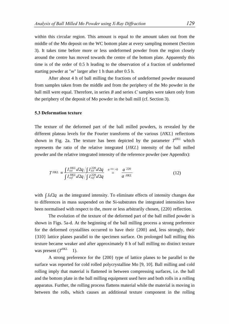
Analysis of Ball Milled Mo Powder using X-Ray Diffraction 129
within this circular region. This amount is equal to the amount taken out from the
middle of the Mo deposit on the WC bottom plate at every sampling moment (Section
3). It takes time before more or less undeformed powder from the region closely
around the centre has moved towards the centre of the bottom plate. Apparently this
time is of the order of 0.5 h leading to the observation of a fraction of undeformed
starting powder at "m" larger after 1 h than after 0.5 h.
After about 4 h of ball milling the fractions of undeformed powder measured
from samples taken from the middle and from the periphery of the Mo powder in the
ball mill were equal. Therefore, in series B and series C samples were taken only from
the periphery of the deposit of Mo powder in the ball mill (cf. Section 3).
5.3 Deformation texture
The texture of the deformed part of the ball milled powders, is revealed by the
different plateau levels for the Fourier transforms of the various {HKL} reflections
shown in Fig. 2a. The texture has been depicted by the parameter THKL which
represents the ratio of the relative integrated {HKL} intensity of the ball milled
powder and the relative integrated intensity of the reference powder (see Appendix):
TI d I d
I d I dHKL tot
HKLtot
refHKL
refHKL
HKL
≡ =∫ ∫∫ ∫
>2 2
2 2
220
220
0 220θ θθ θ
αα
α (12)
with Id∫ 2θ as the integrated intensity. To eliminate effects of intensity changes due
to differences in mass suspended on the Si-substrates the integrated intensities have
been normalised with respect to the, more or less arbitrarily chosen, {220} reflection.
The evolution of the texture of the deformed part of the ball milled powder is
shown in Figs. 5a-d. At the beginning of the ball milling process a strong preference
for the deformed crystallites occurred to have their {200} and, less strongly, their
{310} lattice planes parallel to the specimen surface. On prolonged ball milling this
texture became weaker and after approximately 8 h of ball milling no distinct texture
was present (THKL ≅ 1).
A strong preference for the {200} type of lattice planes to be parallel to the
surface was reported for cold rolled polycrystalline Mo [9, 10]. Ball milling and cold
rolling imply that material is flattened in between compressing surfaces, i.e. the ball
and the bottom plate in the ball milling equipment used here and both rolls in a rolling
apparatus. Further, the rolling process flattens material while the material is moving in
between the rolls, which causes an additional texture component in the rolling

130 Chapter 6
direction of the rolled material, whereas the ball milling process is not expected to
induce any in (surface) plane anisotropy.
6
4
2
0
14121086420ΣH
2
0.5 h 1 h 2 h 4 h
{110
}
{200
}
{211
}
{220
}
{310
}
{321
}
6
4
2
0
14121086420ΣH
2
0.5 h 1 h 2 h 4 h
{110
}
{200
}
{211
}
{220
}
{310
}
{321
}
a) b)
6
4
2
0
14121086420ΣH
2
2 h 4 h 8 h16 h
{110
}
{200
}
{211
}
{220
}
{310
}
{321
}
6
4
2
0
14121086420ΣH
2
8 h 16 h 32 h
{110
}
{200
}
{211
}
{220
}
{310
}
{321
}
c) d)
Fig. 5. Deformation texture parameter THKL as a function of ΣH2 = H2+K2+L2 for
ball milled Mo powders of series Am, Ap, B and C determined from the integrated
intensities of the line profiles of the ball milled powder and of the reference powder
(see Eq. 12).
THKLTHKL
THKLTHKL
Series Am Series Ap
Series B Series C
Analysis of Ball Milled Mo Powder using X-Ray Diffraction 131
The evolution of the texture can be explained as follows. In the initial stage of
ball milling, most particles that deformed were flattened into flakes (cf. Section 5.1)
which after being suspended in isopropanol (in the procedure for specimen
preparation for XRD analysis; cf. Section 3) position onto the Si-substrate with a
strong tendency for their flat sides to be parallel to the surface of the Si-substrate (cf.
Fig. 3b). Upon prolonged ball milling the shape of the deformed powder particles
changed due to the multiple cold welding and fracture processes that took place. Then
large, irregularly shaped agglomerates of particles (cf. Fig. 3c) occurred and no
preferred positioning on the Si-substrate of such particles is expected to take place
during preparation of the XRD specimen. This leads to disappearance of the texture,
as observed through THKL, upon continued ball milling. A similar texture behaviour
was observed upon ball milling Ni3Al powder [11].
Since the Mo powder particles first deformed into flake-like particles and then,
on prolonged ball milling, into irregularly shaped agglomerates of particles, it is
understandable that the amount of undeformed, starting powder dropped to zero
before the texture (related to the amount of flake-like particles) disappeared (cf. Figs.
4 and 5).
5.4 Evolution of structural imperfection
5.4.1 Integral breadth as function of ball milling time
The diffraction-line profiles of the Mo powder particles become broadened
excessively during the ball milling process. As an example the {220} line profiles of
the undeformed starting powder (0 h), also used as reference powder (see Section 4),
and a selection of {220} line profiles of deformed powders are shown in Fig. 6 (after
removal of the background). For relatively short durations of ball milling (0 to 4 h) the
Kα1 and Kα2 peaks are clearly resolved whereas for longer durations of ball milling
no separate Kα1 and Kα2 peaks can be observed.
Since the broadenings of the reflections of the undeformed reference powder
are very small and comparable with the broadenings of a specially made Si-standard
specimen [12], it can be assumed that the line profiles of the reference powder
represent the true instrumental line profiles. Consequently, the Fourier transforms of
the line profiles of the deformed part of the powder, as obtained by application of a
devonvolution procedure, as described in Section 2.2 or 2.3, contain broadening due
to structural causes only. These structural broadenings can be characterized by the
integral breadth (= integrated intensity of the only structurally broadened line profile
divided by its peak height), which, assuming the peak maximum occurs at the origin

132 Chapter 6
chosen in reciprocal space, is equal to the reciprocal value of the area under the
corresponding normalized Fourier transforms [5].
Inte
nsity
(a.
u.)
90898887862θ
0
2
4
8
32
Fig. 6. X-ray diffraction line profiles of {220} Mo reflection of undeformed starting
powder (0 h), also used as reference powder, and ball milled powder for increasing
times of ball milling: 2, 4, 8, 32 h.
The integral breadths of all only structurally broadened line profiles are
presented versus the reciprocal of the distance between the corresponding diffracting
planes, 1/dHKL, in Figs. 7a-d. In general for a certain reflection the integral breadth
increased with ball milling time indicating a more severe lattice deformation if ball
milling time increases. The change of the broadenings for series Am and Ap with ball
milling time deviates somewhat from the general trend and is comparable with the
behaviour of α for these series with ball milling time: compare Figs. 7a, b with Fig. 4.
Therefore, the same type of reasoning holds to understand the behaviour of the
broadening of series Am and Ap with ball milling time (see Section 5.2).
5.4.2 Integral breadth as function of diffraction-vector length
Now consider the results of series B and series C in Figs. 7c and 7d, respectively.
Ignoring the first period of ball milling, the line broadening of each reflection
increased with approximately the same amount if the ball milling time was doubled.
This holds for series B and for series C, and thus up to at least 32 h of ball milling.
º2θ
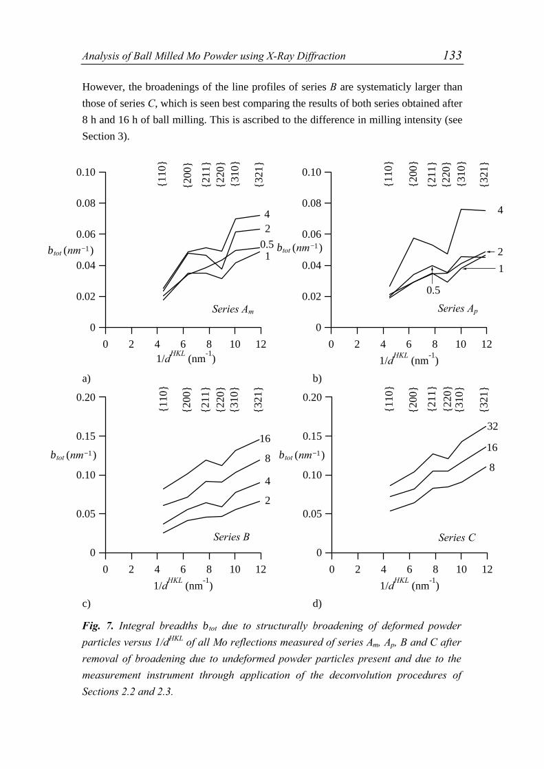
Analysis of Ball Milled Mo Powder using X-Ray Diffraction 133
However, the broadenings of the line profiles of series B are systematicly larger than
those of series C, which is seen best comparing the results of both series obtained after
8 h and 16 h of ball milling. This is ascribed to the difference in milling intensity (see
Section 3).
0.10
0.08
0.06
0.04
0.02
0
β(nm-1
)
1210864201/d
HKL (nm
-1)
0.51
42
{110
}
{200
}
{211
}{2
20}
{310
}
{321
}
0.10
0.08
0.06
0.04
0.02
0
β(nm-1
)
121086420
1/dHKL
(nm-1
)
4
2
1
0.5
{110
}
{200
}
{211
}{2
20}
{310
}
{321
}
a) b)
0.20
0.15
0.10
0.05
0
β(nm-1
)
121086420
1/dHKL
(nm-1
)
4
2
8
16
{110
}
{200
}
{211
}{2
20}
{310
}
{321
}
0.20
0.15
0.10
0.05
0
β(nm-1
)
121086420
1/dHKL
(nm-1
)
16
8
32
{110
}
{200
}
{211
}
{220
}{3
10}
{321
}
c) d)
Fig. 7. Integral breadths βtot due to structurally broadening of deformed powder
particles versus 1/dHKL of all Mo reflections measured of series Am, Ap, B and C after
removal of broadening due to undeformed powder particles present and due to the
measurement instrument through application of the deconvolution procedures of
Sections 2.2 and 2.3.
Series Am Series Ap
Series B Series C
βtot nm( )−1βtot nm( )−1
βtot nm( )−1 βtot nm( )−1

134 Chapter 6
Structural line broadening is usually conceived as the convolution of
broadening due to (i) finite size of the diffracting crystallites (size broadening) and (ii)
local variations in interplanar distance, as due to the presence of lattice defects
inducing strain fields (strain broadening) [6]. If the line profile width is characterized
by the integral breadth β, then in case of pure size broadening β ≡ βS = K/D (for βS in
reciprocal space) with D the mean crystallite size and K a constant close to unity [6],
and in case of pure strain broadening β β≡ =DHKLe d2~ / (for βD in reciprocal space),
with ~e a measure for strain due to the strain fields induced by the lattice distortions
[13] and dHKL as the interplaner distance of lattice planes of the type HKL.
If both types of broadening occur simultaneously, separation of "size" and
"strain" integral breadth components can be performed on the basis of the dependence
of the total integral breadth βtot on the length of the diffraction vector characterized by
1/dHKL using knowledge of the shape of the corresponding component line profiles.
For example, if both component line profiles are assumed to be Cauchy, then the total
integral breadth of the measured line profile, βtot, equals β β βtot = +S D , whereas if
both profiles are assumed to be Gaussian, β β βtot2 2 2= +S D . Then plotting of βtot vs
1/dHKL in case of Cauchy component line profiles or of βtot2 vs 1/(dHKL)2 in case of
Gaussian component line profiles yields straight lines with slopes related to ~e and
intercepts cut from the ordinate related to D.
An overall increase of β as a function of 1/dHKL occurs for all series shown in
Fig. 7. However, systematic deviations of the overall trend occur for specific
reflections. For example after short durations of ball milling (0.5 - 4 h) the integral
breadths of the {200} and {310} reflections are relatively large. One might suggest
that such deviations could be explained by intrinsic anisotropy of the elastic constants
of the material considered: a reflection associated with a relatively "weak"
crystallographic direction would broaden relatively strongly [14]. However, the
anisotropy of the elastic constants of Mo cannot explain the relatively large integral
breadths of the {200} and {310} reflections, since these reflections correspond to
relatively stiff crystallographic directions [15].
To avoid effects on the line-profile analysis of these HKL dependent
deviations, two orders of the same reflection (i.e. {110} and {220}) are used to
separate the contributions due to size and strain. Results obtained assuming Cauchy
shaped component (size and strain) line profiles and K = 1 are shown in Fig. 8. The
crystallite sizes for series Am and Ap are of the order of 100 - 300 nm after ball milling
for 0.5 h to 4 h11. Continued ball milling led to a strong decrease of crystallite sizes to
11 The result of series Am after 0.5 h of ball milling has not been shown because the broadening did notcomply with the assumed type of size-strain separation: i.e. a negative part cut from the ordinateoccurred in the plot of βtot vs 1/dHKL.

Analysis of Ball Milled Mo Powder using X-Ray Diffraction 135
a)
10
2
3
456
100
2
3
456
1000
D (
nm)
0.5 1 2 4 8 16 32 milling time (h)
series Am
series Ap
series B
series C
b)
6x10⁻³
4
2
0
0.5 1 2 4 8 16 32
milling time (h)
series Am
series Ap
series B
series C
Fig. 8. Results of line-profile analysis assuming Cauchy shaped component (size and
strain) line profiles performed on the integral breadth values of the {110} and {220}
Mo reflections of series Am, Ap, B and C depicted in Fig. 7. Particle sizes D obtained
from the intercept of the abscissa are presented in (a) (note the logarithmic scale) and
corresponding microstrain values ~e obtained from the slopes in (b).
~e

136 Chapter 6
20 nm after 32 h of ball milling (series C). This decrease of crystallite size is
accompanied with an increase of the average microstrain to about 0.4 %. Clearly, both
sources of line broadening contribute significantly to the total broadening (see also
Fig. 7). Assuming Gaussian shaped component line profiles led to similar results,
although the average particle size is somewhat smaller and the average strain is
somewhat larger: after 32 h of ball milling a crystallite size of approximately 15 nm
and an average strain of 0.6 % were obtained.
The results of series Am and Ap show a relatively large scatter which is ascribed
to the relatively large sensitivity of the relatively large values of D (in these cases) for
small deviations of the intercept of the ordinate caused by small errors in β and to the
effects of sampling of the powder as discussed in Section 5.2. Note also the small but
systematic difference between the results of series B and series C due to the difference
in milling intensities of these series (see Section 3).
It has been observed [14, 16 - 20] that upon ball milling of powders the
crystallite size would decrease until a certain saturation level is reached. Such a level
could result as a steady state for the competition between grain refinement, due to
plastic deformation, and grain growth/relaxation processes, such as recovery and
recrystallisation [14, 20]. A saturation level for the average microstrain has sometimes
been observed; in other cases the average microstrain reaches a maximum after some
ball milling time but decreases upon further ball milling [14, 16 - 20]. From this work
it seems probable (see Fig. 8) that on prolonged ball milling, i.e. longer than 32 h, the
crystallite size may decrease further and the average microstrain may still increase.
Extrapolation of the results obtained suggest a minimum crystallite size of the order of
10 nm and a maximum average microstrain of the order of 0.4 to 0.6 %. Such values
have been found for other ball milled bcc materials [14, 17 - 20].
5.5 Interpretation of microstrain; determination of dislocation density
It will be shown here that the structural broadening observed can be ascribed to the
presence of deformation induced dislocations. To this end line-profile simulation and
matching has been performed using a new Monte-Carlo-type approach to line-
broadening simulation.
Within a single crystalline sphere of radius R a number of "infinitely long",
straight edge and/or screw dislocations, corresponding to a given dislocation density ρis distributed at random in accordance with the operating glide systems of the
crystalline material considered [21]. Here, only the strain-broadened parts of the
diffraction-line profiles are computed according to the kinematical diffraction theory
as follows. A number of pairs of points is selected at random, such that (i) for each

Analysis of Ball Milled Mo Powder using X-Ray Diffraction 137
pair the vector connecting both points has length L and is parallel to the diffraction
vector considered (L = correlation distance; see Section 4) and (ii) the points of each
pair are located within the sphere of radius R considered. The contributions of all pairs
of points to the real and imaginary "strain" Fourier coefficients (see Eqs. (13) and (15)
in Ref. 13) are calculated taking into account the displacement fields of all
dislocations distributed in the crystal considered. The calculated "strain" Fourier
coefficients are averaged over the total number of pairs. The process of distributing
dislocations on the glide planes and selecting pairs of points is repeated several times
for the same value of L until the average values of the corresponding "strain" Fourier
coefficients become independent of continuation of this procedure. Subsequently, this
calculation procedure is carried out for increasing values of L, until for large L the
"strain" Fourier coefficients become negligibly small. The strain broadened line
profiles thus calculated were characterized by their integral breadths.
The deformation of a body centered cubic crystal (Mo is bcc) can take place
through slip of dislocations along three different glide planes: {110}, {211} and
{321}, with 12 111a⟨ ⟩ as the possible Burgers vectors [22]. Often the contribution of
the {321} glide planes is small and can be neglected [9, 10]. Here, it is assumed that
dislocations are present on the {110} and {211} glide planes only.
As an example, the simulation method was carried out for Mo crystals
containing either screw dislocations or edge dislocations or both types of dislocations,
with in all cases ρ = 1014 m-2. Other parameters were: R = 1 µm, 1000 pairs of points
per correlation distance L and 100 repetitions per correlation distance. The known
descriptions for the displacement fields of edge and screw dislocations in an elasticly
isotropic material were adopted [22] with Poisson's ratio, ν = 0.293, and with the
lattice constant of Mo, aMo = 0.31472 nm. In case of a mixture of edge and screw
dislocations the probability of distributing an edge or a screw dislocation is equal.
Results are shown in Fig. 9 for the same {HKL} reflections as measured
experimentally.
Obviously, the integral breadths of the simulated strain broadened line profiles,
show an overal increase upon increasing 1/dHKL. Because size broadening is absent
(see above) the lines intersecting the points representing the integral breadths of {110}
and {220}, respectively, should go through the origin, as they do. However,
systematic deviations from the overall trend occur in case of presence of only screw
dislocations, whereas in case of presence of only edge dislocations a more or less
linear dependence on 1/dHKL is observed. In case of a mixture of both types of
dislocations the integral breadth shows an intermediate behaviour.

138 Chapter 6
20x10-3
15
10
5
0
β (nm-1
)
1210864201/d
HKL(nm
-1)
edge & screw
edge
screw{1
10}
{200
}
{211
}
{220
}
{310
}
{321
}Fig. 9. Integral breadths of simulated strain broadened line profiles plotted vs 1/dHKL
using either edge dislocations, screw dislocations or a mixture of both types of
dislocations with ρ = 1014 (m-2) and R = 1 µm. Dislocations are distributed at
random compatible with the {110} and {211} glides planes of Mo and with12 111aMo ⟨ ⟩ as the Burgers vector.
The displacement fields used in the calculations for edge and screw
dislocations pertain to elastically isotropic material and therefore the {HKL}-
dependence of the integral breadth in Fig. 9 in the case of only screw dislocations is
solely caused by the crystallographic direction dependence of the displacement and
strain fields of the dislocations with respect to the diffraction vectors considered.
Thus, possible anisotropy of the elastic constants of the Mo crystal does not play a
role here. Corresponding {HKL} dependence has been considered earlier using a
different approach [23 -25].
Comparing the simulated integral breadth dependence on 1/dHKL (Fig. 9) with
the experimentally obtained results after short durations of ball milling (cf. Figs. 7a
and b: 1, 2 and 4 h) similar observations are made: e.g. in both cases the integral
breadths of the {200} and {310} are relatively large. This suggests strongly that the
presence of dislocations is the cause of the experimentally observed dependence of βon 1/dHKL. After longer times of ball milling the integral breadths of the
experimentally measured {200} and {310} reflections become relatively less

Analysis of Ball Milled Mo Powder using X-Ray Diffraction 139
pronounced, which could be interpreted according to Fig. 9 as that the fraction of
screw dislocations becomes smaller and, consequently, the fraction of edge
dislocations becomes larger.
10x10-3
7.5
5
2.5
0
10x107 86420
edgeedge/screw
screw
Fig. 10. Microstrain estimate ~e versus square root of dislocation density ρ obtained
from line-profile analysis assuming Cauchy shaped line profiles of simulated strain
broadened {110} and {220} Mo reflections. Dislocations are either of edge type,
screw type or a mixture of both types and are distributed at random compatible with
the {110} and {211} glide planes of Mo, with 12 111aMo ⟨ ⟩ as the Burgers vector and
with R ρ = 10.
The simulations [21] show that β ρD is practically a univocal function of
R ρ . Variations in the value taken for R ρ lead to changes in βD at constant ρ of,
say, 50 % for 1 10≤ ≤R ρ and < 10 % for 10 25≤ ≤R ρ . To arrive at an estimate
for the dislocation density in the deformed part of the ball milled powders, for the
present simulations R ρ has been set equal to 10. The strain-broadened diffraction-
line profiles were calculated for increasing dislocation densities with either pure edge,
pure screw or a mixture of edge and screw dislocations. Then, corresponding average
microstrain values ~e were determined assuming Cauchy or Gaussian shaped
component lines profiles using the integral breadths of the {110} and {220} only.
Results are presented in Fig. 10 for the case of Cauchy shaped component line
ρ ( )m−1
~e

140 Chapter 6
profiles. A linear relation between ~e and the square root of the dislocation density is
observed. For the same dislocation density, edge dislocations cause a somewhat larger
value of ~e than screw dislocations. Estimates of dislocation densities in the deformed
part of the ball milled powder were obtained from the experimental average
microstrain values ~e (Fig. 8b) and the ~e -ρ relation shown in Fig. 10. Results are
presented in Fig. 11 applying a mixture of edge and screw dislocations for all series.
The influence of the type of dislocations on the dislocation densities determined is
relatively small. It follows that during the ball milling process the dislocation density
increases to values of about 3 × 10¹⁵ m-2 after 32 h of ball milling in case of Cauchy
component line profiles (to 7 × 10¹⁵ m-2 in case of Gaussian component line profiles):
these values correspond to a severely cold deformed material.
5x10¹⁵
4
3
2
1
0
ρ (m-2
)
0.5 1 2 4 8 16 32milling time (h)
series Am
series Ap
series B series C
Fig. 11. Estimates of dislocation densities ρ of series Am, Ap, B and C using ~e (from
Fig. 8b), as obtained from line-profile analysis assuming Cauchy shaped component
(size and strain) line profiles performed on the integral breadth values of {110} and
{220} Mo reflections (see Fig. 7), and ~e (from Fig. 10), as obtained from the same
analysis performed on integral breadth values obtained from simulated {110} and
{220} strain broadened Mo reflections.

Analysis of Ball Milled Mo Powder using X-Ray Diffraction 141
6. Conclusions
– During ball milling of Mo powder in a low-energy ball mill several stages of
deformation can be identified. In a first stage the generally soft, powder particles are
flattened due to action of compressive forces. The ball milled powder consists of a
mixture of undeformed powder particles and flake-like, deformed powder particles.
The flakes have more or less flat faces preferably parallel to {100} planes of the
crystal lattice. Continued ball milling causes the amount of flake-like deformed
powder particles to decrease, and simultaneously more and more irregularly shaped
agglomerates of particles occur, as a result of multiple cold welding and fracturing of
powder particles.
– X-ray diffraction methods developed in this study allow quantitative determination
of the (still) undeformed part of the ball milled powder from the Fourier transform of
reflections from the ball milled powder obtained after deconvolution using
corresponding reflections from the initial powder. This analysis is possible also if
texture is present in the specimen prepared for diffraction analysis. Such texture can
occur due to the presence of the flake-like particles that tend to orient their flat faces,
preferably parallel to {100} of the crystal lattice of Mo, parallel to the surface of the
diffraction specimen, in dependence on the procedure used for preparation of the
specimen for diffraction analysis.
– Analysis of the ball milling induced structural imperfections from the occurring
diffraction-line broadening revealed a drastic decrease of the size of the diffracting
crystallites upon ball milling down to 10 - 20 nm, i.e. values much smaller than the
size of the irregularly shaped agglomerates of particles observed at this advanced state
of ball milling. Simultaneously the internal average microstrain increased up to 0.4 -
0.6 %.
– The dominant source of structural line broadening are dislocations generated by ball
milling: line-profile simulation and matching revealed a dependence of structural line
broadening on the length of the diffraction vector as observed experimentally. The
nature of the dislocations becomes less screw-like and more edge-like upon continued
ball milling. In an advanced stage of ball milling the dislocation density becomes as
large as 3 - 7 × 10¹⁵ m-2.
Acknowledgements
This work has been part of the research program of the Foundation for Fundamental
Research on Matter (Stichting FOM), The Netherlands. Financial support was also
provided by the Netherlands Technology Foundation (STW). The authors are indebted

142 Chapter 6
to Dr. H. Bakker for providing the ball milling facilities, to Dr. G. Rixecker for
performing the ball milling experiments and to ing. E.J.M. Fakkeldij for operating the
SEM.
AppendixRelation between THKL and ααHKL
After short times of ball milling the diffracting volume pertaining to the {HKL}
reflection consists of a mixture of undeformed powder particles of total volume VundefHKL
and deformed powder particles of total volume VdefHKL . The volume weighted intensity
distribution of the line profile of the {HKL} reflection, I totHKL (2 )θ , is described by Eq.
(2). The integrated intensity of this reflection, I dtotHKL 2θ∫ , can be expressed as
I d V V I dtotHKL
undefHKL
defHKL HKL2 2θ θ= +∫ ∫( ) (A. 1)
with I dHKL 2θ∫ the integrated intensity of the line profile of the {HKL} reflection per
unit of volume. It has been assumed that I dHKL 2θ∫ is independent of the state of
deformation of the powder particles, i.e. I d I d I dundefHKL
defHKL HKL2 2 2θ θ θ= =∫ ∫ ∫ .
If the integrated intensity of an arbitrary {HKL} reflection is divided by that of
the {220} reflection it follows, using Eq. (5), that
I d
I d
V V
V V
I d
I dtotHKL
tot
undHKL
defHKL
und def
HKL2
2
2
2220 220 220 220
θθ
θ
θ∫∫
∫∫
=+
+=
∫∫
αα
θ
θ
220
220 220
2
2HKL
undefHKL
undef
HKLV
V
I d
I d. (A. 2)
If the undeformed powder of the ball milled powder is equal to the reference
powder (the same morphology, microstructure and texture; implying the same
procedure for (diffraction) specimen preparation for both specimens), then, according
to Eq. (8)
V
V
V
VundefHKL
undef
refHKL
ref220 220= (A. 3)
and Eq. (A. 2) can be written as

Analysis of Ball Milled Mo Powder using X-Ray Diffraction 143
I d
I d
V
V
I d
I dtotHKL
totHKL
refHKL
ref
HKL2
2
2
2220
220
220 220
θθ
αα
θ
θ∫∫
∫∫
= . (A. 4)
Since V I drefHKL HKL 2θ∫ represents the integrated intensity of the {HKL}
reflection of the reference specimen, V I d I drefHKL HKL
refHKL2 2θ θ∫ ∫= , Eq. (A. 4)
becomes
I d
I d
I d
I dtotHKL
totHKL
refHKL
ref
2
2
2
2220
220
220
θθ
αα
θ
θ∫∫
∫∫
= . (A. 5)
Recognizing the parameter THKL from Eq. (12) it follows from Eq. (A. 5)
I d
I d
I d
I dT
totHKL
tot
refHKL
refHKL
HKL2
2
2
2220 220
220θθ
θ
θαα
∫∫
∫∫
= = . (A. 6)
References
[1] A.W. Weeber, H. Bakker, Physica B 153 (1988) 93.
[2] E.Hellstern, H.J. Fecht, Z. Fu, W.L. Johnson, J. Appl. Phys. 65 (1989), 305.
[3] E.Hellstern, H.J. Fecht, Z. Fu, W.L. Johnson, J. Mater. Res. 4 (1989), 1292.
[4] T.C. Bor, M.C. Huisman, R. Delhez, E.J. Mittemeijer, Mat. Sci. For. Vol. 278-281
(1998), 145.
[5] R.N. Bracewell, The Fourier Transform and its Applications, McGraw-Hill, Tokyo, 1978.
[6] B.E. Warren, X-Ray Diffraction, Addison Wesley, Reading, Mass., 1969.
[7] A.J.C. Wilson, Acta Cryst. 23 (1967), 888.
[8] R. Delhez, E.J. Mittemeijer, J. Appl. Cryst. 8 (1975), 612.
[9] D. Raabe, K. Lücke, Mat. Sci. For. Vol. 157-162 (1994), 597.
[10] Y.B. Park, D.N. Lee, G. Gottstein, Acta. Mat. 46 (10), (1988), 3371.
[11] L. Lutterotti, S. Gialanella, Acta Mater. 46, (1), (1998), 101.
[12] J.G.M. van Berkum, G.J.M. Sprong, Th.H. de Keijser, R. Delhez and E.J. Sonneveld,
Powder Diffraction 10 (1995), 129.
[13] R. Delhez, Th.H. de Keijser and E.J. Mittemeijer, Fresenius Z. anal. Chem. 312 (1982),
1 - 16.
[14] I. Börner, J. Eckert, Mat. Sci. & Eng. A 226-228 (1997), 541.
[15] C.J. Smithells (editor), Metals Reference Book, 5th edition, Butterworths, London, 1976.
[16] P.S. Gilman, J.S. Benjamin, Ann. Rev. Mater. Sci., Vol. 13, (1983), 279.
[17] C.C. Koch, Nanostruc. Mat. 2 (1993), 109.
[18] D. Oleszak, P.H. Shingu, J. Appl. Phys. 79 (6), (1996), 2975.

144 Chapter 6
[19] W.M. Kuschke, R.M. Keller, P. Grahle, R. Mason, E. Arzt, Z. Metallk. 86 (1995), 12.
[20] H.H. Tian, M. Atzmon, Acta Meta. 4 (1999), 1255.
[21] J.-D. Kamminga, R. Delhez, to be published.
[22] F.R.N. Nabarro, Theory of Crystal Dislocations, Oxford University Press, Oxford, 1967.
[23] M. Wilkens, Phys. Stat. Sol. (a) 2 (1970), 359.
[24] I. Groma, T. Ungár, M. Wilkens, J. Appl. Cryst. 21 (1988), 47.
[25] A.C. Vermeulen, R. Delhez, Th.H. de Keijser, E.J. Mittemeijer, J. Appl. Phys. 77 (10),
(1995), 5026.

Summary
Lattice imperfections, such as dislocations and misfitting particles, shift and/or
broaden X-ray diffraction (XRD) line profiles. Most of the present analysis methods
of the shift and broadening of XRD line profiles do not provide the characteristics of
lattice imperfections. The main part of this thesis deals with a new approach to the
analysis of broadened and shifted XRD line profiles that does not have the limitations
of the present analysis methods. The approach is based on micromechanical modelling
of the microstructure of the material. A small volume which is representative of the
microstructure of the material is used to model and calculate the materials behaviour
on a local scale incorporating the (strain fields of the) lattice imperfections.
Subsequently, the behaviour of this representative element can be used to calculate the
overall materials properties. X-ray diffraction-line profiles are calculated from such
model materials and are compared with the measured ones. By adjusting the
parameters of the micromechanical model, the calculated line profiles can be matched
to the experimental ones. In this way characteristics of the microstructure of the
experimental material can be determined and subsequently overall materials properties
can be predicted. Hence, a direct link between XRD line-profiles characteristics and
materials properties is conceivable.
The new diffraction-line profile calculation approach is developed in chapters
2 and 3 for a two-dimensional model composite material containing a periodic
distribution of misfitting particles. The shifts and broadenings of line profiles in
absence of particle-matrix misfit are studied in chapter 2. The line-profile broadenings
of matrix reflections are caused by finite distances in the matrix between the (non-
diffracting) particles ("size" broadening). Relations between the "size" broadening of
the matrix line profiles and model parameters, such as the particle fraction, the particle
size and the degree of particle clustering, are established. If a misfit between particles
and matrix exists the matrix line profiles are also broadened due to the strain field
induced by the particles in the matrix ("strain" broadening). A simple method is
proposed to separate the "size" and "strain" contributions to the total broadening.
The line-profile shifts and broadenings due to “strain” alone are analyzed in
two steps in chapter 3. First, the relations between model parameters, such as the
particle size, the particle fraction, the particle-matrix misfit and the degree of particle
clustering, and the mean strain of the matrix and root mean square strain of the matrix
are studied. Due to the ordering of the particles in the composite material the strain
field in the matrix is direction dependent which is reflected in the root mean square
strain of the matrix. Then, the relations between the values that characterize the matrix
146 Summary
strain and the shift and width of the calculated line profiles are investigated. The mean
matrix strain, calculated on the basis of the shift of the line-profile centroid of the
simulated XRD line profile, shows approximately equal behaviour for all values of the
model parameters as the mean strain calculated from the strain field in the matrix. The
broadening of the simulated XRD line profiles reflects the direction dependence of the
strain field in the matrix. This leads to the observation that for all values of the model
parameters the line-profile broadenings are proportional to the product of the centroids
of the line profiles and the root mean square strains in the specific crystallographic
directions (as usually assumed in practice). Thus for the particle-matrix systems
studied here the influence of the various model parameters on the line-profile position
and width can be explained directly from the influence of these model parameters on
the mean strain and root mean square strain of the matrix material.
Verification of the results of the novel simulation approach can be
accomplished, for example, by studying the same material employing a different
experimental technique, such as Transmission Electron Microscopy. The study of
particle/matrix systems using this technique is the topic of chapter 4. The strain field
in the matrix due to misfitting particles causes, under certain diffraction conditions,
diffraction contrast lobes in bright field and dark field images to appear. Information
on the particle-matrix misfit and/or on the particle dimensions can be obtained by an
analysis of the extent of the contrast lobes. The classical analysis is unreliable for
specimen foils that contain a high number density of misfitting particles and/or that
are relatively thin (smaller than five times the extinction distance). An alternative
method is proposed here that does not have the limitations of the classical method.
The extent of the contrast lobes is characterized by the distance of the maximum or
minimum intensity of the contrast lobes in bright field and dark field to the center of
the misfitting particle. For the interpretation of the observed contrast lobes a model
system, consisting of a single disc-shaped misfitting particle placed centrally in a thin
specimen, is considered. The contrast lobes in bright and dark field images are
calculated as a function of, in particular, the particle radius, the foil thickness and the
particle thickness. Simultaneous fitting of calculated bright and dark field diffraction
contrast images to the experimental ones leads to determination of the particle misfit
and the local thickness of the specimen foil. The method is illustrated for a nitrided
Fe-2 at. % V alloy with small disc-shaped VN precipitates and leads to a consistent
interpretation in terms of particle size and misfit upon precipitation. The foil thickness
values determined by diffraction contrast analysis agree well with data obtained from
an independent thickness measurement technique.
Summary 147
In chapters 5 and 6 attention is paid to powder particles that have been
deformed in a ball milling device. Ball milling provides a route for the preparation of
non-equilibrium material that may possess unusual chemical and physical properties.
In this work the ball milling process in a low energy ball mill is investigated as a
function of milling time and using Mo powder as a model material. After relatively
short times of ball milling still undeformed Mo powder particles are present in the
type of ball mill used. A method is developed, on the basis of line-profile
deconvolution, that enables the determination of the volume fraction of undeformed
powder particles and the (Fourier transform of the) line profile of the deformed
particles. The accuracy of these results are largely determined by the effect of counting
statistical intensity variations. A region in Fourier space can be indicated for which the
determination of the volume fraction of undeformed Mo powder is optimal.
During the deformation of the Mo powder particles several stages can be
identified. First, the particles are flattened due to compressive forces of the bouncing
ball in the mill. These flat particles exhibit a deformation texture which is comparable
with that of rolled polycrystalline Mo. On prolonged ball milling all powder particles
are eventually deformed and agglomerates of particles are formed without exhibiting a
specific shape. The crystallite size decreases towards 10 - 20 nm, the apparent texture
disappears and internal strains are built up to microstrain levels of the order of 0.4 -
0.6 %.
From the magnitude of the microstrains an estimate of the dislocation density
can be calculated using a simple three dimensional model of the distribution of
dislocations in deformed Mo powder particles. It assumes that straight edge and/or
screw dislocations are distributed at random on the {110} and {211} glide planes of
Mo with ⟨ ⟩111 as possible Burgers vector directions. The X-ray diffraction line
profiles are obtained using a Monte-Carlo type of line-profile calculation method. A
comparison of the integral breadths of several simulated and experimental line profiles
clearly indicates the presence of dislocations in the ball milled Mo powder particles.
Then the dislocation density is estimated to become as large as 3 7 1015− ⋅ m-2 in an
advanced state of ball milling, which indicates a severely cold deformed material.

148 Summary

Samenvatting
Roosterfouten, zoals dislocaties en mispassende deeltjes, verschuiven en/of verbreden
röntgendiffractielijnprofielen. De meeste lijnprofiel-analysemethoden zijn niet in staat
om uit de gemeten lijnprofielverschuiving en -verbreding roosterfouten goed te
karakteriseren. Dit is jammer, omdat roosterfouten een belangrijke rol spelen bij het
gedrag en de eigenschappen van kristallijne materialen. Het grootste gedeelte van dit
proefschrift gaat daarom over een nieuwe methode voor de analyse van verschoven en
verbrede lijnprofielen. De methode is gebaseerd op het berekenen van lijnprofielen op
basis van een micromechanisch model van het gemeten materiaal. Dit model
beschrijft het gedrag van dit materiaal in een representatief volume-element waarin de
beteffende roosterfouten en de, met hun aanwezigheid samenhangende, rekvelden
worden opgenomen. Hieruit kunnen bijvoorbeeld ook de overall
materiaaleigenschappen berekend worden. Van dit modelmateriaal worden
lijnprofielen berekend en deze kunnen vergeleken worden met de gemeten
lijnprofielen. Door nu de parameters van het modelmateriaal te variëren, kunnen de
berekende lijnprofielen worden gefit aan de gemeten lijnprofielen. Op deze manier
kan informatie worden verkregen over de microstructuur van het gemeten materiaal.
Dus, een directe relatie tussen karakteristieken van röntgendiffractielijnprofielen en
materiaaleigenschappen is denkbaar.
De nieuwe lijnprofielberekeningsmethode wordt beschreven in hoofdstukken 2
en 3 voor een tweedimensionaal model-composietmateriaal dat een periodieke
verdeling van mispassende deeltjes bevat. De verschuiving en verbreding van lijn-
profielen in afwezigheid van mispassing tussen deeltjes en matrix worden in hoofd-
stuk 2 bestudeerd. De lijnprofielverbreding van matrixreflecties wordt veroorzaakt
door eindige afstanden tussen de (niet-diffracterende) deeltjes ("size"-verbreding).
Relaties zijn bepaald tussen deze "size"-verbreding van de matrix lijnprofielen en
modelparameters, zoals de deeltjesfractie, de deeltjesgrootte en de mate van deeltjes-
clustering. Als er een mispasing tussen deeltjes en matrix bestaat, worden de lijn-
profielen van de matrixreflecties ook verbreed tengevolge van het rekveld in de matrix
veroorzaakt door het mispassende deeltje ("strain"-verbreding). Een eenvoudige
methode is voorgesteld om de "size"- en "strain"-bijdragen aan de totale verbreding
van elkaar te scheiden.
De lijnprofielverschuiving en -verbreding tengevolge van "strain" zijn in twee stappen
geanalyseerd in hoofdstuk 3. Eerst zijn de relaties tussen modelparameters, zoals de
deeltjesgrootte, deeltjesfractie, mispassing tussen deeltjes en matrix en de mate van
clustering van de deeltjes, en de gemiddelde rek en het gemiddelde van het ordening

150 Samenvatting
van de deeltjes in het composietmateriaal is het rekveld in de matrix
richtingsafhankelijk, hetgeen in dit geval alleen tot uiting komt in het gemiddelde
kwadraat van de rek in de matrix. Vervolgens zijn de relaties tussen de karakteristieke
matrixrekwaarden en de verschuiving en verbreding van de berekende lijnprofielen
onderzocht. De gemiddelde rek, berekend op basis van de verschuiving van de
centroïde van het lijnprofiel, vertoont een ongeveer gelijk gedrag voor alle
onderzochte waarden van de modelparameters als de gemiddelde rek berekend uit het
rekveld in de matrix. De verbreding van het berekende lijnprofiel weerspiegelt de
richtingsafhankelijkheid van het rekveld in de matrix. Dit leidt tot de waarneming dat
voor alle waarden van de modelparameters de lijnprofielverbreding evenredig is aan
het produkt van de lijnprofielcentroïde en het gemiddelde kwadraat van de rek in de
specifieke kristallografische richting (zoals vaak aangenomen in de praktijk). Dus
voor het hier bestudeerde deeltjes/matrix-systeem is de invloed van de verschillende
modelparameters op de lijnprofielpositie en -verbreding direct te verklaren vanuit hun
invloed op de gemiddelde rek en het gemiddelde kwadraat van de rek in de matrix.
Verificatie van de resultaten van de nieuwe simulatiemethode is mogelijk door
hetzelfde materiaal met een andere experimentele techniek te bestuderen, zoals TEM.
De studie van deeltje/matrix-systemen met behulp van deze techniek is het onderwerp
van hoofdstuk 4. De rekvelden in de matrix, tengevolge van de mispassende deeltjes,
veroorzaken onder zekere (diffractie) condities, zogenaamde diffractiecontrastlobben
in helderveld- en donkerveldopnamen. Informatie over de deeltjes/matrix-mispassing
en/of de deeltjesafmetingen kan worden verkregen door de uitgebreidheid van de
lobben te bestuderen. De klassieke methode bleek niet betrouwbaar voor
preparaatfolies met een hoge deeltjesdichtheid en/of kleine foliedikte. Vandaar dat een
alternatieve methode is voorgesteld. De uitgebreidheid van de contrastlobben is
gekarakteriseerd door de afstand tussen de maximum of minimum intensiteit van de
contrastlobben in helderveld en donkerveld tot het midden van de mispassende
deeltjes. Om de contrastlobben te kunnen interpreteren is een modelsysteem gebruikt,
bestaande uit een schijfvormig, mispassend deeltje in het midden van een dun
preparaatfolie. De contrastlobben in helder- en donkerveld zijn berekend als functie
van, met name, de deeltjesstraal, de foliedikte en de deeltjesdikte. Door nu tegelijker-
tijd de berekende helderveld- en donkerveldbeelden te fitten op de experimentele
beelden kunnen de deeltjesmispassing en de locale preparaatfoliedikte bepaald
worden. De methode is geïllustreerd aan de hand van een genitreerde Fe-2 at.% V
legering met kleine schijfvormige VN-precipitaten en leidt tot een consistente
interpretatie van de deeltjesgrootte en deeltjes/matrix-mispassing. Bovendien komen

Samenvatting 151
de op deze wijze bepaalde foliediktes goed overeen met waarden die met een andere
foliediktemeettechniek zijn bepaald.
In hoofdstukken 5 en 6 is aandacht besteed aan poederdeeltjes die zijn
vervormd in een kogelmolen. Kogelmalen maakt het mogelijk niet-evenwichts-
materialen te maken, die buitengewone chemische of fysische eigenschappen bezitten.
In dit werk is het kogelmaalproces in een lage-energie kogelmolen bestudeerd als
functie van de maalduur en met Mo-poeder als modelmateriaal. Na relatief korte
maalduren blijkt er in de door ons gebruikte kogelmolen nog onvervormd Mo-poeder
aanwezig te zijn. Er is een methode ontwikkeld, op basis van lijnprofieldeconvolutie,
om de volumefractie onvervormd poederdeeltjes en de Fouriertransform van het
lijnprofiel van de gedeformeerde deeltjes te bepalen. De nauwkeurigheid van de
resultaten blijkt sterk afhankelijk van de invloed van telstatistiek. In de Fourierruimte
kan een gebied aangegeven worden waar de volumefractie onvervormd Mo-poeder
optimaal bepaald kan worden.
Het deformeren van Mo-poeder verloopt in verschillende stadia. Eerst worden
de deeltjes geplet tengevolge van de samendrukkende krachten van de stuiterende bal
in de kogelmolen. Deze geplette deeltjes vertonen een deformatietextuur die vergelijk-
baar is met die van gewalst polykristallijn Mo. Na langduriger malen worden
uiteindelijk alle Mo-deeltjes vervormd en ontstaan agglomeraten van deeltjes zonder
voorkeursvorm. De kristallietgrootte neemt af tot 10 - 20 nm, de textuur verdwijnt en
microrekken ontstaan met een grootte tot 0.4 - 0.6 %.
Een schatting van de dislocatiedichtheid op basis van de microrekwaarden kan
worden gemaakt met een eenvoudig driedimensionaal model van de distributie van
dislocaties in gedeformeerde Mo-poederdeeltjes. Aangenomen wordt dat rechte rand
en/of schroef-dislocaties random verdeeld zijn op de {110} en {211} glijvlakken van
Mo met ⟨ ⟩111 als mogelijke richtingen van de Burgersvector. De
röntgendiffractielijnprofielen worden berekend met een Monte-Carlo-type lijnprofiel-
berekeningsmethode. Een vergelijking van de integrale breedte van verschillende
gesimuleerde en experimentele lijnprofielen duidt duidelijk op de aanwezigheid van
dislocaties in de gekogelmaalde Mo-poederdeeltjes. De dislocatiedichtheid wordt
geschat op 3 7 1015− ⋅ m-2 in een vergevorderd stadium van kogelmalen, hetgeen duidt
op een behoorlijk zwaar koudvervormd materiaal.


Nawoord
De afgelopen jaren heb ik het voorrecht gehad om in twee wetenschappelijke groepen
aanwezig te zijn. Dit heeft zo z'n voor- en nadelen. Twee groepen betekent twee
professoren met elk hun eigen visie, opvattingen en wijze van schrijven. Het betekent
ook ruwweg tweemaal zoveel collega's, vakgroepsvoordrachten èn vakgroepsborrels.
Twee groepen met elk hun eigen sfeer, maar beide met een grote gedrevenheid voor
het doen van onderzoek. Ik heb me er thuis gevoeld en daarvoor dank ik eenieder.
Dit onderzoek kon niet zonder Eric Mittemeijer en Erik van der Giessen met hun niet
aflatende inzet en grote betrokkenheid. Het onderzoek kon ook niet zonder Rob
Delhez, die de dagelijkse begeleiding op zijn eigen, prettige, wijze vorm gaf. Dit geldt
ook voor Staf de Keijser, die echter door omstandigheden gedwongen werd de
begeleiding eerder te beëindigen.
Delen van dit proefschrift zijn ontstaan in samenwerking met de afstudeerders
Antoine Kempen en Marc Huisman. Hun aanwezigheid en inzet betekende niet alleen
een belangrijke bijdrage aan dit proefschrift, maar vooral een zeer prettige tijd van
samenwerken en samenouwehoeren.
Dit onderzoek kon ook niet zonder de kennis en kunde van vele collega's en
medewerkers binnen en buiten beide vakgroepen. Mensen bedankt! Daarnaast dank ik
ook de PCM, de lasgroep en de instrumentmakerij voor de gezelligheid en de
"mogelijkheden" buiten het gewone werk om.
Tot slot wil ik mijn ouders en vrienden bedanken voor hun warme belangstelling,
steun en begrip in de afgelopen jaren. Als laatste dank ik Jet voor haar liefde en steun,
zeker voor die momenten waarop het nodig was.


Curriculum Vitae
Teunis Cornelis Bor
Geboren op 14 december 1969 te Schoonrewoerd
1982 - 1988 VWO, Koningin Wilhelmina College te Culemborg
1988 - 1994 Studie Materiaalkunde aan de Technische Universiteit Delft.
Afgestuurd (met lof) in de sectie Lastechnologie en Niet-Destructief
Onderzoek onder begeleiding van Prof.dr. G. den Ouden op het
onderwerp "Het diffusielassen van Si3N4 met een Ni-tussenlaag".
1994 - 1999 Onderzoeker in Opleiding in de sectie Fysische Chemie van de Vaste
Stof, Laboratorium voor Materiaalkunde en de sectie Micromechanica
van Materialen, Laboratorium voor Technische Mechanica, Technische
Universiteit Delft.
Promotie-onderzoek onder begeleiding van dr.ir. R. Delhez, dr.ir. Th.H.
de Keijser (tot 1997), prof.dr.ir. E. Van der Giessen en prof.dr.ir. E.J.
Mittemeijer, op het onderwerp "Strain Fields in Crystalline Solids,
Prediction and Measurement of X-Ray Diffraction Patterns and
Electron Diffraction Contrast Images".
1999 - Post-doctoraal onderzoeker in de sectie Fysische Chemie van de Vaste
Stof, Laboratorium voor Materiaalkunde en de sectie Micromechanica
van Materialen, Laboratorium voor Technische Mechanica, Technische
Universiteit Delft. Onderwerp: Berekening en interpretatie van
röntgendiffractielijnverbreding van materialen met dislocaties.
1999 - Research and Development Tricycle Cross