Department of Economics and Finance

University of Guelph

Discussion Paper 2017-08

Strategic advance sales, demand uncertainty and

overcommitment

By:

Sebastien Mitraille and Henry Thille

Strategic advance sales, demand uncertainty and

overcommitment

Sebastien Mitraille∗

Toulouse Business School

E-mail: s.mitraille@tbs-education.fr

Henry Thille

University of Guelph

E-mail: hthille@uoguelph.ca

November 17, 2017

Abstract

We study a game in which producers can sell in two periods: one before a randomdemand is fully revealed and one after. This type of game corresponds to models of strategicforward trading or of advance sales to intermediaries or consumers. Demand variations andcommitted advance sales results in the possibility that the net residual demand in the finalstage may be so low that it is not profitable for producers make additional sales, or indeed,may even drive the final period price to zero, introducing some convexity into producers’payoffs. If this possibility of ex post overcommitment occurs on the equilibrium path, itreduces the level of advance sales chosen by producers, muting the pro-competitive effectsfound under deterministic demand. We establish a condition that determines whether ornot demand uncertainty is “minor”, in the sense that the equilibrium depends only on theexpected value of the demand shock. In addition, we demonstrate that when the support ofdemand shocks is narrow enough compared to the marginal cost of production, there existsa unique symmetric subgame-perfect equilibrium in pure strategies. When the support ofdemand shocks is wider, we establish a regularity condition on the distribution of demandshocks and the model parameters that ensures the existence of a unique equilibrium in purestrategies. We illustrate through examples that commonly used uni-modal distributionssatisfy this condition, while bi-modal distributions may not.

JEL Classification: C72, D43, L13Keywords: Oligopoly, advance sales, uncertainty, overcommitment

Acknowledgement: The authors thank for their useful comments Rene Kirkegaard, KurtAnnen, Asha Sadanand, James Amegashie and seminar participants at the University of Guelph;Sergei Izmalkov, Rabah Amir, and participants of the Oligoworkshop 2016 (Universite de Paris- Dauphine); Philippe Chone, Laurent Linnemer, Thibaud Verge, and seminar participants atCREST-LEI; Simon Cowan and participants of the RES 2017 conference (University of Bristol).

∗Corresponding author

1

1 Introduction

The ability of firms to commit to sales in advance of market clearing creates a strategic incentiveto capture future demand through these advance sales. This leads to market outcomes that aremore competitive than what occurs when advance sales are prohibited since producers are unableto commit to not make additional sales in the future when the market clears. Examples includefirms selling through forward contracts and firms selling to consumers or other intermediarieswho then store for future consumption or resale. However, if the future demand is uncertainat the time the advance sales commitment is made, producers face the risk that they may haveover-committed sales if demand turns out to be lower than expected. In this case, producers mayfind that further spot sales are unprofitable, in which case the strategic incentive for advancesales is likely to be muted as they have no effect on rivals spot sales in these subgames.

We analyze the effects of this possibility of ex-post overcommitment on the equilibrium ofan advance sales game in which producers can commit to sell a quantity in a period prior tothe meeting of the spot market and subsequently can produce additional output in the periodin which the spot market meets. We find that the degree of uncertainty (as measured by thesize of the support of the distribution of demand), as well as the shape of the density of demandshocks, have important consequences on the nature of the equilibrium and on its existence.This particular feature is due to the fact that in dynamic games like ours, in which producerscan sell both before and after uncertainty is resolved, degenerate equilibria may occur in somesub-games, in the sense that given the realized shock and the strategies chosen in the pastsome or all producers may choose to not produce at all in the sub-game. Particular attentionmust then be paid to whether or not these subgame equilibria are on the equilibrium path.1

While it is possible that spot sales or price can be zero in our model, one contribution of thispaper is to determine when these situations arise on the equilibrium path and to characterizethe importance of this phenomenon for existence and nature of a pure strategy equilibrium.

We show that there are three qualitatively different types of equilibria: equilibria in whichadditional spot sales are made in every subgame (which we label “type I”); equilibria in whichspot sales are not made in some subgames, but price is positive in every subgame (“type II”);and equilibria in which both spot sales and price are zero in some subgames (“type III”). Wedistinguish demand distributions with a narrow support, for which the equilibrium can onlyinvolve strictly positive spot prices (type I or II), from those with wide support for which theequilibrium can involve zero spot price as well (type III). Our main results are the following.In our first theorem, we establish that a unique pure-strategy equilibrium exists in the narrowsupport case for any distribution of demand shocks. When the lower bound on the support of thedistribution of demand shocks is limited, spot sales are always strictly positive at equilibrium(type I) and demand uncertainty has no qualitative effect on the equilibrium in the sensethat only the expected value of demand matters to oligopolists. In this sense, uncertainty is“minor” when the equilibrium is of type I. For more extreme lower bounds on the support ofthe distribution of demand shocks, spot sales can be nil in some subgames on equilibrium pathand a type II equilibrium is the outcome: advance sales balance the usual strategic effects withthe possibility that they are the sole source of profit obtained when demand is low.

In the wide support case, the possibility of a zero spot price results in the potential forpayoffs to be convex. Our second theorem deals with this case, and establishes the existenceof a unique pure-strategy equilibrium under a regularity assumption on the distribution of thestochastic component of demand and the other model primitives.2 This theorem establishes

1In a paper that generalizes the proof of existence and uniqueness of the classical static Cournot equilibriumto encompass the case of degenerate equilibria, Gaudet and Salant [11] point out, as a potential application, theimportance of these equilibria when they occur in sub-games.

2Absent this regularity condition, multiple solutions to the first order condition of each firm may co-exist, andthe best response in pure strategy may lack continuity. In the case where the regularity condition is not satisfiedand the support of demand shocks is wide enough, the game still possesses an equilibrium in mixed strategy due

2

that the condition under which the equilibrium involves only strictly positive spot sales (typeI) is the same as in the narrow support case, so we can classify uncertainty ‘minor’ in the sameway in the wide support case. When this condition is violated the equilibrium involves zerospot sales or even zero spot prices, i.e., is either type II or III. As our regularity assumptiondepends on marginal cost and the number of firms in addition to the demand distribution,neither the log-concavity of the density of demand shocks, nor an increasing hazard rate, issufficient to satisfy the regularity assumption.3 We establish in a series of examples that bi-modal distributions with modes located “close” to the extreme of the support of shocks fail tosatisfy our regularity assumption, while common uni-modal distributions tend to satisfy it.

Our model can be seen as capturing the essential features of a number of different approachesthat examine the incentives that producers have to sell to consumers in advance. One of theseis the literature on strategic forward contracting following Allaz and Vila [2] (See Allaz [1],Thille [29], Ferreira [8], Mahenc and Salanie [19], Liski and Montero [17]) in which producersmay enter binding forward contracts prior to the meeting of the spot market. In Allaz andVila [2] since future demand is known with certainty, it does not matter whether the forwardcontracts are for cash settlement (the counter-parties simply exchange cash depending on thedifference between the forward and spot prices) or physical delivery (the producer actuallydelivers the contracted quantity to the forward purchaser, who then resells on the spot market).While this distinction does not matter when spot demand is certain, when demand is uncertainthis equivalence may break down as with physical delivery the committed production may turnout to be “too large” ex-post.4 Popescu and Seshadri [25] analyze a strategic forward tradingmodel with stochastic demand drawn on a support unbounded from above, where the minimalinverse demand intercept can be as low as the unit cost of production. The importance ofthe demand support on the nature of equilibrium, as well as the consequences of the shapeof the density of shocks on the existence of an individual best response, are not analyzed. Ina model of supply function competition with costless production, Holmberg and Willems [13]show that forward contracts in the form of an infinite series of options can be used by duopolistsin equilibrium to commit their supply function on the spot market to have a negative slope,that is to commit to reduce competition. They establish this result in a costless productionmodel, assuming that the hazard rate of the distribution of demand shocks either increases oris not too decreasing. In our model, where a single forward contract is used but production iscostly, we show that existence of an equilibrium does not rely on assuming that the distributionof demand shocks has an increasing hazard rate (in the case where an assumption is needed).

A second approach to modelling strategic advance sales has producers selling physical pro-duction to other agents in a period prior to the spot market. Anton and Das Varma [3], Dudine,Hendel and Lizzeri [7], and Guo and Villas-Boas [12] study the effect of consumers storage onimperfect competition (respectively on a duopoly, on a monopoly, or in the case of differenti-ated products, but all in the absence of demand uncertainty). By increasing production in aperiod, producers cause a lower price which induces consumers to buy and store for a futureperiod, lowering that future period’s demand. Whereas a monopoly would prefer to let theprice increase to limit consumer storage, a duopoly is better off encouraging consumers storageto compete more fiercely in the short run. In a similar vein, Mitraille and Thille [21, 22] studya model where speculators may purchase production in an earlier period, store the good, andthen resell in the spot market5. Whereas demand uncertainty is one of the salient features of

to the continuity of the expected payoffs (See Fudenberg and Tirole [10])3With the exception that in the case of costless production, an increasing hazard rate distribution satisfies

our assumption and hence, is sufficient to guarantee the existence of an equilibrium.4Allaz [1] allows for uncertainty in the strategic forward contracting game, but he does not allow for the

possibility that firms may decide to produce no additional output for the spot market, or that the spot pricemight be driven to zero.

5Mitraille and Thille [21, 22] have multiple spot markets as well, but the forces at work are essentially thesame.

3

their model, they assume a limited capacity of storage or that small quantities can always beprofitably produced by oligopolists, to rule out unprofitable spot sales from the equilibriumpath. By inducing speculative purchases producers essentially are capturing future sales as theproduction sold to speculators returns as another source of supply in the future spot market.Our model can be viewed as capturing the essential features of these models: by selling inadvance producers lower the net demand they face in the future.

In addition, our model is related to the analysis of static Cournot competition when quanti-ties must be chosen before a random demand is known. Klemperer and Meyer [14] examine thechoice between price and quantity competition in this setting, but essentially focus on ‘minor’demand uncertainty only. However in the presence of larger uncertainty on the demand inter-cept, it is known that firms’ individual payoffs can be a convex function of their sales, as wellas those of their competitors. Lagerlof [16] considers the problem of an oligopoly facing a lineardemand with a random intercept which can take two values, high or low. He shows that multipleequilibria may be present due to the non-concavity induced by the possibility of a zero priceoccurring when demand is low.6 In our model, the possibility to sell once demand is revealed isendogenous, and enriches the set of equilibria while modifying the conditions required for theexistence of an equilibrium: it introduces strategic considerations for selling in advance,7 butalso provides oligopolists with an option to adjust sales by increasing them ex-post if a highenough demand stated is revealed.

The commitment to advance sales along with the possibility to make additional spot salesin our model is also reminiscent of the literature on the value of flexibility when uncertaintyaffects a commitment.8 In this literature, the timing of a single production period is endogenous,and production can happen either before or after uncertainty is realized. The focus is then onwhether or not the first mover advantage survives the introduction of uncertainty, or on whetherentry deterrence may occur. For example, Spencer and Brander [28] study the trade-off betweenproduction prior to the realization of uncertainty, where a firm gains Stackelberg leadership atthe possible cost of overproduction, and production after the realization of uncertainty, inwhich a risk-free Cournot equilibrium obtains. In contrast, our approach supposes symmetry ofmoves and allows possible production in every period, so both ex-ante commitment and ex-postadaptation are possible. In this context we discuss the existence and the nature of subgameperfect Nash equilibria, which is not addressed in [28] and others.

We next present our model, followed by the determination of equilibrium in both the narrowand wide support cases. We then provide some examples of demand distributions and costs thatboth meet and fail our regularity condition.

2 The Model

Our model consists of two markets that meet in consecutive periods: an advance sales marketin period one and a spot market in period two. We model the advance sales market as onein which producers make binding commitments to supply the product to competitive agents.9

These advance sales can be of two general types: first, physical production occurs in period one

6Lagerlof [15] extends this analysis to consider a continuous distribution of demand shocks.7In these papers, additional sales after demand is revealed are not possible (with the exception of the price

competition case in Klemperer and Meyer [14]), so that there is no strategic effect of the advance sales.8See Appelbaum and Lim [4], Perrakis and Warskett [24], Vives [31], Spencer and Brander [28], and Sadanand

and Sadanand [26].9Advance sales differ from advance production as defined in the models of Saloner [27] and Pal [23] in that in

the former, the marginal revenue firms face when going on the “spot” market is residual one, while in the laterfirms are made more aggressive on the “spot” market due to the production realized they sell entirely when themarket opens. In advance production games, the cost structure is crucial to the outcome of the game: equilibriacan be asymmetric as a firm carrying a leader production is committed to sell it forcing its competitor to behaveas a follower, but symmetric outcomes are also possible (Saloner [27]); cost differences between periods, such asdiscounting, then matters to equilibrium selection (Pal [23]).

4

and the advance sales are delivered to the purchasers at that time, who then store at no costfor use in period two; and, second, forward contracts are entered in which settlement occurs byphysical delivery of the contracted quantity10. Either way, net spot market demand faced byproducers is reduced by the quantity of advance sales. Consumption occurs only in period twoand is supplied by the sum of advance sales and any further production undertaken in periodtwo.

There are n producers, indexed by i = 1, ..., n, who interact over two periods, t = 1, 2. Att = 1, each producer may choose a quantity xi which is sold to competitive agents and has theeffect of reducing net demand faced by producers at t = 2. The price in the advance sale marketis p1. Let x = (x1, x2, ..., xn), X =

∑ni=1 xi, and X−i =

∑j 6=i xj . In period two, each producer

may choose to produce an additional quantity yi to sell on the spot market at a price p2. Wedefine Y =

∑ni=1 yi and Y−i =

∑j 6=i yj .

Firms face the same linear production costs in each period,11 so the total cost of productionis given by C(xi, yi) = c(xi + yi), with c ≥ 0. Defining p1 and p2 as the price in each period,and assuming a discount factor equal to one,12 the total profit for a producer is then

πi = (p1 − c)xi + (p2 − c)yi. (1)

Consumers’ demand demand in the spot market is assumed to be linear in the market pricep2,

D(p2; a) = max{a− p2, 0}, (2)

where a ∈ R+ is random with a continuous and differentiable cumulative distribution functionF (a) and density f(a). It is realized at the beginning of period two and observed by all agentsat that time. The support of F (a) is the interval [aL; aH ] ⊆ R+, which is assumed to allowproduction and sales to be always potentially profitable, in the sense that if demand whereknown, some production would take place:13

c ≤ aL ≤ aH ≤ +∞. (3)

We assume that all agents observe the n-tuple of advance sales,14 x, as well as the realization ofa before they make their choices in period two. The inverse demand for the spot sales in periodtwo is then

P (Y,X, a) = max{a− (X + Y ), 0}. (4)

We assume free disposal if X exceeds a.

10The counterparty to the forward contract receives the quantity specified in the forward contract and thenresells it (if a “speculator”) or consumes it.

11Linear production costs are necessary to be able to interpret the model as being consistent with both forwardtrading with physical delivery and competitive storage since splitting production across periods has no effect oncost. Convex production costs would give firms an additional cost-smoothing incentive to produce in the secondperiod and would cloud the effect that we wish to analyze. In the same way, the constant marginal cost is thesame in each period so that there is no inherent advantage in production costs between advance and spot sales.

12A unit discount factor means that the timing of the receipt of profits does not matter to a firm. This isimportant to be able to interpret xi as either advance sales made in period one (with revenue and costs realizedin period one) or as forward contracts with physical delivery (with revenue and costs realized in period two).

13As such, we do not consider the risk that demand would be so low that firms would regret any productionat all.

14Observability of advance sales matters in our setting, as it does more generally in all commitment games.Indeed the possibility of exerting some (endogenous) leadership through advance sales could be jeopardized ifthey are not observable. Bagwell [6] establishes that in a (textbook) Stackelberg game, non-observability of theleader’s choice results in the Cournot outcome being the sole pure strategy equilibrium to the game. HoweverVan Damme and Hurkens [30] demonstrate that a mixed strategy equilibrium close to the Stackelberg outcomeexists in Bagwell’s game, and Maggi [18] proves that private information restores the value of commitment. Inthe context of strategic forward trading, Ferreira [9] shows that imperfect observability can lead to multipleequilibria, including some that are even more competitive than in Allaz [2].

5

Demand for advance sales in period one is derived from the expectation of p2. The per-unitexpected profit to an advance purchase is E[p2|X] − p1, where E[p2|X] is the expectation ofp2 conditional on the quantity of advance sales made. The competitive and rational agentspurchasing the advance sales drive this expected profit to zero. Consequently, we have

p1 = E[p2|X], (5)

which represents the inverse demand faced by producers in the period one advance sales market.From (1) it is clear that advance sales affect the marginal profit of spot sales only through

the effect of aggregate advance sales on p2. This allows us to restrict our attention to spot salesstrategies that only depend on X instead of the entire vector of individual advance sales, x. Astrategy for a firm consists of a pair ωi = {xi, yi(X, a)} with xi ∈ R+, and yi : R+ × [aL; aH ]→R+. The spot sales strategy for a firm, yi(X, a), represents how the firm will play in subgameswhere total advance sales are X and the state of demand is a. The expected payoff for any firmi = 1, ..., n given strategies for each producer is then

E(πi(ω1, ..., ωn)) = E[p2|X]xi +

∫ aH

aL

P

(n∑i=1

yi(X, a);X, a

)yi(X, a) dF (a)− c(xi + yi(X, a)).

(6)We look for the subgame-perfect equilibria of this game, with x∗i and y∗i (X, a), i = 1, ...n,denoting the equilibrium strategies.

3 Subgame equilibrium and expected profit

We now establish the subgame equilibrium and expected payoff firms face when choosing theiradvance sales. We determine conditions on model parameters for which qualitatively differenttypes of subgame equilibria are possible on the equilibrium path. In particular, we determineconditions under which there is a non-zero probability of zero spot sales and a non-zero probabil-ity of a zero spot price. This distinction matters as when these events occur off the equilibriumpath, they do not affect firms’ choices of advance sales, while when they occur on equilibriumpath they must be taken into account. Once the correct expression of firms individual expectedprofit is obtained, the equilibrium to the game can be determined.

3.1 Spot market equilibrium in period two

At the beginning of period two, all agents observe the realization a, as well as X. Each firmsolves

maxyi≥0{(P (Y,X, a)− c)yi + (p1 − c)xi} , (7)

where the second term represents the profits from advance sales which are sunk and have noeffect on the choice of spot sales. The equilibrium spot sales in this subgame are straightforwardto determine:

y∗i (X, a) = max

[a−X − cn+ 1

, 0

], i = 1, ...n, (8)

which is the usual Cournot equilibrium adjusted for the reduction in demand due to the advancesales. The equilibrium spot price depends on whether or not spot sales are positive, but alsomust respect the non-negativity constraint on price: demand may turn out so low that it cannotaccommodate the total advance sales. Consequently, we have

p∗2(X, a) =

0 if a ≤ X

a−X if X ≤ a ≤ X + c

(a−X + nc)/(n+ 1) if a > X + c

(9)

6

with the first line representing a binding non-negativity constraint on price, and the secondline representing a binding non-negativity constraint on spot sales. If neither non-negativityconstraint binds, the price is simply the Cournot equilibrium price when demand is reduced bythe total quantity of advance sales.

3.2 Expected price and profits of the advance sales game

In period one, agents make decisions based on their expectations over the outcomes in the periodtwo subgames. Inverse demand for firms’ advance sales is given by (5) and producers chooseadvance sales to optimize their expectation of profit, (1), with yi and p2 replaced by (8) and(9). From (9) we see that the probability that period two price will be zero depends on X. IfX < aL, then p2 > 0 in all subgames, while if X ≥ aL there are subgames in which p2 = 0.Consequently, a positive second period price occurs when a > max[aL, X]. Similarly, from (8)we see that if X < aL− c, then yi > 0 in all subgames, while if X ≥ aL− c, there are subgamesin which yi = 0. Consequently, positive spot sales occur for a > max[aL, X + c] . As rationalagents use this information in forming expectations we have the following general expressionfor the expected price in period one,

p1 = E[p∗2(X, a)|X] =

∫ max[aL,X+c]

max[aL,X](a−X)dF (a) +

∫ aH

max[aL,X+c]

a−X + nc

n+ 1dF (a). (10)

As the qualitative nature of the equilibrium depends on whether or not a zero price or zero spotsales outcome is possible, we define the alternative types of equilibria as follows:

Definition 1 Given equilibrium advance sales of X∗, we say that the equilibrium is of

• Type I if Pr[p∗2(X∗, a) = 0] = 0 and Pr[y∗i (X

∗, a) = 0] = 0,

• Type II if Pr[p∗2(X∗, a) = 0] = 0 and Pr[y∗i (X

∗, a) = 0] > 0, and

• Type III if Pr[p∗2(X∗, a) = 0] > 0 and Pr[y∗i (X

∗, a) = 0] > 0.

In a Type I equilibrium the non-negativity constraints for the spot price and spot sales do notbind for any possible realization of a. In a Type II equilibrium the non-negativity constraint forthe spot price does not bind for any a while there are some possible realizations of a for whichspot sales are zero. Finally, in a Type III equilibrium there are realizations of a for which bothspot price and sales are zero.

We can further refine our understanding of the possibility of a zero price by noting that allaggregate advance sales larger than aH − c are strictly dominated, as the price for the maximaldemand would be below the marginal cost of production c for all demand states, and hencewill not be chosen by producers. This implies that we only need to consider X ≤ aH − c.Consequently, if aL > aH − c, the probability of a zero spot price is nil for any X potentiallyplayed by producers, that is for any X not strictly dominated. The equilibrium cannot be ofType III in this case. This observation motivates the following definition:

Definition 2 F (a) has narrow support if aH−aL ≤ c and has wide support if aH−aL > c.

If F (a) has narrow support only equilibria of Type I or II are possible, while if F (a) has widesupport Type III equilibria must be considered. Clearly, if c = 0 or aH = +∞ only the widesupport case can occur.

We are now in a position to compute the expected profit for a firm in period one incorporatingthe equilibrium in the period two subgames, which we denote πe(xi, X−i). Using y∗i (X, a) andp∗2(X, a) from (8) and (9) in (1) we have

πe(xi, X−i) = E[(p∗2(xi +X−i, a)− c)(xi + y∗i (xi +X−i, a))]. (11)

7

The precise calculation of the expectation in (11) depends on whether F (a) has narrow orwide support. In the case of a narrow support for F (a) we have after some simplification15

πe(xi, X−i) =

{πeI(xi, X−i) if 0 ≤ X ≤ aL − cπeII(xi, X−i) if aL − c < X ≤ aH − c.

(12)

where

πeI(xi, X−i) =

∫ aH

aL

(a−X − cn+ 1

)(xi +

a−X − cn+ 1

)dF (a) (13)

and

πeII(xi, X−i) =

∫ c+X

aL

(a−X − c)xi dF (a) +

∫ aH

c+X

(a−X − cn+ 1

)(xi +

a−X − cn+ 1

)dF (a) (14)

When F (a) has wide support, we have to account for the possibility of a zero price in periodtwo when advance sales are relatively large. In this case we have

πe(xi, X−i) =

πeI(xi, X−i) if 0 ≤ X ≤ aL − cπeII(xi, X−i) if aL − c < X ≤ aLπeIII(xi, X−i) if aL < X ≤ aH − c

(15)

where πeI(xi, X−i) and πeII(xi, X−i) are defined in (13) and (14) respectively, and

πeIII(xi, X−i) =

∫ X

aL

−cxidF (a) +

∫ c+X

X(a−X − c)xidF (a)

+

∫ aH

c+X

(a−X − cn+ 1

)(xi +

a−X − cn+ 1

)dF (a) (16)

We next determine the existence of a pure-strategy equilibrium to the game in the narrowand wide support cases respectively.

4 Narrow support

When F (a) has narrow support it is possible to prove the existence of a unique symmetricequilibrium in pure strategies for any F (a). We do this by demonstrating that i) expectedprofit is concave in xi given X−i, and ii) the resulting unique best response is strictly decreasingand continuous.

Consider the case xi ≤ aL − c − X−i in which the expected profit is given by πeI(xi, X−i).The marginal effect of an increase in advance sales is given by

∂πeI(xi, X−i)

∂xi=

(n− 1)(E[a]− c)− 2nxi − (n− 1)X−i(n+ 1)2

, (17)

which is strictly decreasing in xi. This expression, which holds if advance sales are smallenough, characterizes the expected marginal profit of selling in advance when it affects spot

15Specifically, from (9) we use

p∗2(X, a)− c =

−c if a ≤ X

a−X − c if X ≤ a ≤ X + c

(a−X − c)/(n+ 1) if a > X + c

8

sales in all subgames, i.e., for all possible realizations of demand.16 This case corresponds to anequilibrium of Type I and if a symmetric equilibrium is of this type we denote x∗I the solution

in x of∂πeI (x,(n−1)x)

∂xi= 0, which can be determined in closed form as

x∗I =(n− 1)(E[a]− c)

n2 + 1. (18)

Next, consider aL − c −X−i < xi ≤ aH − c −X−i for which πeII(xi, X−i) defines expectedprofit. Again, differentiating with respect to xi we obtain

∂πeII(xi, X−i)

∂xi=

∫ c+X

aL

(a− c− 2xi −X−i)dF (a) +

∫ aH

c+X

(n− 1)(a− c)− 2nxi − (n− 1)X−i(n+ 1)2

dF (a)

=F (c+X) (E[a | a ≤ X + c]− c− 2xi −X−i)

+ (1− F (c+X))((n− 1)(E[a | a ≥ X + c]− c)− 2nxi − (n− 1)X−i)

(n+ 1)2. (19)

An equilibrium of this type is Type II and we denote x∗II a solution in x of∂πeII(x,(n−1)x)

∂xi= 0,

which cannot generally be determined in closed form. In this case, expected marginal profit isa weighted average of the effect on profit in subgames where no spot sales are made (the firstterm in (19)) and the effect on profit in subgames where spot sales are positive (the second termin (19)). The weights are the probabilities that subgames are reached for which y∗(X, a) = 0,F (c + X), and for which y∗(X, a) > 0, 1 − F (c + X). Marginal expected profit from advancesales corresponds to Cournot marginal profit in the subgames where y∗(X, a) = 0 and to (17)in subgames where y∗(X, a) > 0. So (19) represents a weighted average of Cournot behaviouron the advance sales market and of strategic advance sales behaviour with the weights beingthe probabilities of spot sales being zero and positive respectively. We see that the possibilityof zero spot sales reduces the weight given to the strategic incentive to increase advance sales,suggesting that x∗II ≤ x∗I . We can now state the following theorem:

Theorem 1 When F (a) has narrow support, there exists a unique symmetric equilibrium inpure strategies. The equilibrium individual advance sales level is given by

i) x∗I if aL > a (type I),

ii) x∗II if aL ≤ a (type II),

with a = (n2−n)n2+1

E[a] + (n+1)n2+1

c.

Proof: See appendix.‖

Theorem 1i) demonstrates that for given values of n and c, as long as the smallest possiblerealizations of a are sufficiently high, equilibrium advance sales depend on the expected valueof a alone (no other characteristics of F (a) matter). In this case, even if demand turns out tobe the lowest possible, firms will still make additional spot sales in period two: y∗i (nx

∗I , a) >

0. Conversely, Theorem 1ii) demonstrates that when the lowest possible demand states aresufficiently low equilibrium advance sales take into account the possibility that spot sales maybe unprofitable as reflected in the dependence of (19) on E[a | a ≤ X + c] and F (X + c).The possibility that price falls below the marginal cost of production in period two forces firmsto consider the effects of sub-games in which their sales come from advance sales only. Inthis case, equilibrium quantities are not solely based E[a] but depend more generally on othercharacteristics of F (a) as indicated in (19).

16This is the result corresponding to Allaz and Vila [2], with E[a] substituted for the demand intercept.

9

A striking feature of Theorem 1 is that the only assumption we have made regarding F (a)is that it is continuous and differentiable, no other restriction on F (a) is required. This is incontrast with the findings of Popescu and Seshadri [25] or Holmberg and Willems [13], whoobtain closely related uniqueness results by requiring the distribution of shocks to have anincreasing hazard rate. However Popescu and Seshadri consider the wide support case only,while Holmberg and Willems impose costless production in the context of supply functioncompetition, which is equivalent to require a wide support as we discussed above.17 This isalso absent from the analysis by Mitraille and Thille [22], who study a model with a quadraticcost of production that effectively rules out the case of non-profitable production for spot sales.Moreover Theorem 1 also quantifies, in the context of the advance sales competition model westudy, the notion of “minor” uncertainty for which, following conventional wisdom, the resultsof the literature are qualitatively unaffected by uncertainty. Uncertainty can be consideredminor if the lower bound on the support of the distribution is not too low relative expectedvalue: aL > a.

It is important to demonstrate that the condition under which a Type II equilibrium obtains,aL < a, can be satisfied for feasible values of the parameters, i.e., that it does not define anempty set in the parameter space. Since we assume aL ≥ c, part ii) of Theorem 1 is possible

only if c < (n2−n)n2+1

E[a] + (n+1)n2+1

c. As this is violated for n = 1 a monopolist does not find itselfin a situation where spot sales are unprofitable. Indeed, it is clear from (18) that a monopolistwould not sell in advance at all. However, for n > 1, this condition reduces to c < E[a], which istrue under our assumption that c ≤ aL. Consequently, the set of parameters for which a TypeII equilibrium occurs is not empty for n ≥ 2,18 and we have

Corollary 1 A Type II equilibrium does not occur for n = 1, whereas for n ≥ 2 there is anon-empty set of feasible parameters for which a Type II equilibrium obtains.

Furthermore, existence of a Type I equilibrium requires aL > a = (n2−n)n2+1

E[a] + (n+1)n2+1

c.Whether or not this inequality can be satisfied depends on the model primitives. To see this,subtracting c from both sides we have aL−c > n2−n

n2+1(E[a]−c). As n increases, n

2−nn2+1

approachesone and the inequality cannot hold since aL < E[a]. Furthermore, as c approaches aL frombelow, aL− c approaches zero while E[a]− c remains strictly positive, and again this inequalitycannot hold. In summary we have

Corollary 2 The equilibrium may be is of Type I for c and n sufficiently small. For either clarge enough relative to aL or n sufficiently large, the equilibrium can only be Type II.

The implication of Theorem 1 and Corollaries 1 and 2 is that the existing pro-competitiveeffects of advance sales identified in the literature may be tempered once uncertainty overfuture demand is allowed. Indeed, (19) indicates that x∗II < x∗I . Since firms only care about thestrategic effect of advance sales in subgames for which spot sales are positive, x∗II lies betweenthe Cournot level and x∗I when 1 − F (X∗ + c) < 1. While we have shown that equilibriumadvance sales may be lowered by allowing for uncertain demand, it is instructive to investigatethe magnitude of this effect. We do so by computing equilibrium advance sales for a particularexample: a Uniform distribution for a with support [1 − δ, 1 + δ]. In this case, E[a] = 1 andwe can control the type of equilibrium by varying δ. To respect the assumption that aL ≥ c wemust have δ ≤ 1 − c and to have a narrow support requires δ ≤ c/2, so we limit attention toδ ∈ (0,min[c/2, 1 − c]). Setting c = 2/3, δ ∈ (0, 1/3) satisfies these restrictions. For the casen = 3, we plot equilibrium advance sales relative to x∗I in Figure 1 to illustrate the proportionalreduction in advance sales that occurs when the equilibrium is of Type II. A Type I equilibrium

17See Definition 2 and its discussion.18Of course if we relax this assumption, allowing aL < c, there are clearly demand states at which firms would

not produce more in period two for any level of advance sales. In this case the equilibrium can only be of TypeII.

10

occurs in this example for aL = 1− δ ≥ a, or δ ≤ 1− a = 1− 1315 ' 0.13. Limited variations of

demand around its mean does not change the equilibrium level of advance sales, and we see howδ ≡ 1 − a, illustrated as a vertical line, delineates an area in which the extent of uncertaintyover demand is “minor” in that firms only consider E[a] in their choices. However, for δ > δ theequilibrium is of Type II and advance sales are lower. For the largest value of δ consistent witha narrow support (δ = 1/3), advance sales are nearly 40% lower than in a Type I equilibrium,demonstrating that the effect of the possibility of making zero spot sales in period two can besubstantial.

5 Wide support

We turn now to the wide support case, aH − aL > c, allowing for the possibility of a Type IIIequilibrium with a non-zero probability of a zero price in period two. We demonstrate belowthat in this case, the expected profit may be convex in xi on the interval [aL−X−i, aH−c−X−i].Continuity of the best response functions is therefore not guaranteed.19 Moreover, advance salesof a firm and of its competitors are not necessarily strategic substitutes in this case, allowingthe possibility that best responses may not decline monotonically.

To obtain the existence of a unique continuous and decreasing best response function, andhence of a unique symmetric equilibrium, we add two conditions on the model primitives, whichdeal with the existence and slope of the best response respectively. The first condition statesthat if the expected profit is convex for some xi ∈ [aL − X−i, aH − c − X−i], the marginalexpected profit is negative at these points. The second condition states that if the partialderivative of the marginal expected profit with respect to X−i is positive for some xi ∈ [aL −X−i, aH − c − X−i], then the marginal expected profit is also negative at these points. Thatis under the conditions we introduce below, neither convexity issues of the expected profit, norstrategic complementarity of a firm’s advance sales with its competitors’, will interfere withthe individual optimum of each firm; rather these issues will occur elsewhere in the domain ofchoices of each firm which is not part of an equilibrium, although not strictly dominated in thegame-theoretical sense.20

5.1 Equilibrium

The marginal expected profit for X < aL has the same functional form as in the narrow supportcase, with the exception that the range over which (19) applies is reduced. In particular, (17)applies for X ≤ aL− c, while (19) applies for aL− c < X ≤ aL. For aL < X ≤ aH − c marginalexpected profit is given by

∂πeIII(xi, X−i)

∂xi= −cF (X) +

∫ c+X

X(a− c− 2xi −X−i)dF (a)

+

∫ aH

c+X

(n− 1)(a− c)− 2nxi − (n− 1)X−i(n+ 1)2

dF (a),

= −cF (X) + (F (c+X)− F (X)) (E[a | X ≤ a ≤ X + c]− c− 2xi −X−i)

+ (1− F (c+X))(n− 1)(E[a | a ≥ X + c]− c)− 2nxi − (n− 1)X−i

(n+ 1)2(20)

which highlights the tradeoffs a firm makes when choosing advance sales. When increasing itsadvance sales, a firm increases the likelihood of a zero price in period two which is captured

19See also Lagerlof [15, 16] in the context of static Cournot games with demand uncertainty.20The additional condition we impose therefore implies that the expected profit is “single-peaked” in xi for

every X−i, i.e. is quasi-concave in xi for every X−i. Mas-Colell, Whinston, and Green [20] proposition 8.D.3.(p. 253) establishes that normal form games with continuous and quasi-concave payoffs have pure strategy Nashequilibrium, and apply it to static models of oligopoly (section 12.C).

11

by the first term in (20). As p∗1 = E[p∗2(X, a)|X], this results in a lower price for advance salessince the advance purchasers face the risk that their purchase will be valueless in period two.This effect reduces further the incentive firms have to capture future demand through advancesales. An equilibrium in this case is of Type III and we denote by x∗III a solution in x of∂πeIII(x,(n−1)x)

∂xi= 0.

The existence of a unique pure strategy equilibrium of Type III is complicated by thepotential for expected profit to be non-concave when aL < X ≤ aH − c. Differentiating (20)with respect to xi and simplifying gives

∂2πeIII(xi, X−i)

∂x2i= xif(X)− nxif(c+X)

n+ 1− 2(1− F (X))

+2(n2 + n+ 1)

(n+ 1)2(1− F (c+X)) (21)

with the positive first and last terms potentially leading to a convex payoffs. We can express(21) as

∂2πeIII(xi, X−i)

∂x2i= A(X)xi + 2B(X) (22)

whereA(X) = f(X)− n

n+ 1f(c+X) (23)

and

B(X) = −(1− F (X)) +n2 + n+ 1

(n+ 1)2(1− F (c+X)). (24)

We have B(X) < 0,21 however A(X) > 0 is possible, so concavity of πeIII in xi for a given X−iis not assured. Similarly, the derivative of the expected marginal profit with respect to X−i is

∂2πeIII(xi, X−i)

∂xi∂X−i= xif(X)− n

n+ 1f(c+X)xi − (1− F (X))

+n2 + n+ 2

(n+ 1)2(1− F (c+X)), (25)

which we write as∂2πeIII(xi, X−i)

∂xi∂X−i= A(X)xi + B(X), (26)

where

B(X) = −(1− F (X)) +n2 + n+ 2

(n+ 1)2(1− F (c+X)). (27)

While B(X) < 0,22 marginal expected profit may be increasing in X−i as A(X) > 0 cannotbe ruled out, causing the possibility that best response functions may slope upward. Both ofthese potential problems for the existence of a unique pure-strategy equilibrium are due to thepossibility that A(X) > 0.

Nonetheless, these problems may be innocuous at the individual optimum of any firm, andhence at equilibrium, as long as the model parameters and the density f(a) are regular enough.In order to state our condition we define two sets. First, the set of advance sales for a firm forwhich expected profit is concave in xi given X−i when xi +X−i > aL is

S1(X−i) ≡ {xi ∈ [max(aL −X−i, 0), aH − c−X−i] : A(xi +X−i)xi +B(xi +X−i) < 0}. (28)

21Indeed 1 − F (X) ≥ 1 − F (c + X) (with strict inequality for c > 0), and (n2 + n + 1)/(n + 1)2 < 1. Hence

(1− F (X)) > n2+n+1(n+1)2

(1− F (X + c)) and B(X) < 0.22The argument is similar to footnote 21, with the exception that n2+n+2

(n+1)2≤ 1 for n ≥ 1.

12

Second, the set of advance sales for a firm for which marginal expected profit is decreasing inrivals’ output in this case is

S2(X−i) ≡ {xi ∈ [max(aL −X−i, 0), aH − c−X−i] : A(xi +X−i)xi + B(xi +X−i) < 0}. (29)

We make the following assumption:

Assumption 1 (Regularity) The model primitives, c, n, and F (a), are such that for X−i ∈[0, aH − c], S1(X−i) and S2(X−i) are convex sets and, if non-empty, contain their lower bound,max(aL −X−i, 0).

Assumption 1 has the effect of limiting the number of changes in sign of ∂2πeIII/∂x2i and

∂2πeIII/∂xi∂X−i as xi is varied for a given X−i to be at most one. The requirement thatS1 and S2 contain their lower bound if non-empty implies that convexity of expected profit willonly occur for relatively large values of individual, and hence aggregate, advance sales, i.e., forxi close to aH − c−X−i.

Assumption 1 imposes conditions on the number of firms, the marginal cost of production,and the distribution of demand shocks. Neither a distribution with an increasing hazard rate,nor more generally a log-concave distribution, necessarily satisfy it.23 To see this, if we denoteh(a) = f(a)/(1−F (a)) as the hazard rate, we can write the second order derivatives of expectedprofit as

∂2πeIII(xi, X−i)

∂x2i= f(X)

(xi −

2

h(X)

)− f(c + X)

(nxin+ 1

− 2(n2 + n+ 1)

(n+ 1)2h(X + c)

)(30)

and

∂2πeIII(xi, X−i)

∂xi∂X−i= f(X)

(xi −

1

h(X)

)− f(c + X)

(nxin+ 1

− n2 + n+ 2

(n+ 1)2h(X + c)

), (31)

whose sign cannot be fixed by an assumption on the hazard rate alone, except in the particularcase of costless production. When c = 0, f(X) can be factored in (30) and (31), and anincreasing hazard rate h(X) is sufficient to satisfy Assumption 1.24

We can now state the following:

Theorem 2 When F (a) has wide support, under Assumption 1 there exists a unique and sym-metric equilibrium in pure strategies. Furthermore, the equilibrium is Type I if aL > a andeither Type II or III otherwise, where a is as defined in Theorem 1.

Proof: See appendix.‖

The proof of Theorem 2 demonstrates that under Assumption 1 if a firm’s best response toX−i results in xi +X−i > aL then it is in S1(X−i) and S2(X−i), i.e., expected profit is concaveat the best response, which is itself decreasing in X−i. The proof of Theorem 1 establishedthat the expected profit is concave for any xi < aL − X−i, so the assumption that S1(X−i)contains aL −X−i if it is non-empty implies that any non-concavity of expected profit occurs

23Bagnoli and Bergstrom [5] provide a detailed literature review of articles that use an increasing hazard rate orlog-concavity assumption on the distribution of random preferences of buyers in order to establish the existenceof pure-strategy equilibria. They show that log-concavity and and an increasing hazard rate are closely related:log-concavity of a PDF implies log-concavity of a CDF, which implies that the hazard rate of the distribution isincreasing; however a distribution with an increasing hazard rate is not automatically log-concave.

24In this case, (30) is of the same sign as xin+1− 2n

(n+1)2h(xi+X−i)and (31) is of the same sign as xi

n+1−

n−1(n+1)2h(xi+X−i)

. Both of these expressions are monotonically increasing in xi for a given X−i and so satisfy

Assumption 1. See also Holmberg and Willems (2015).

13

for large values of xi. The largest value of xi considered by firms is xi = aH − c−X−i for whichthe marginal expected profit is negative. If the expected profit is convex at this point, thenthe marginal expected profit is increasing, which implies that the marginal expected profit isnegative wherever the expected profit is convex and the existence of a pure strategy equilibriumis assured. The same argument is used to show that convexity of S2(X−i) implies that strategiccomplementarity, which occurs when expected marginal profit increases with X−i, can occuronly where the expected marginal profit is negative i.e. only for advance sales in excess of thebest response. Consequently, the best response function is continuous and decreasing whichthen implies uniqueness of the pure strategy equilibrium.

Theorem 2 establishes that the the definition of ‘minor’ uncertainty that was established inTheorem 1 remains the same in the wide support case. When aL > a, equilibrium advance salesand price depend only on E[a] and are not affected by any other characteristics of F (a).

For aL < a the equilibrium is either of Type II or III. We can partially characterize whichtype obtains by demonstrating that a type III equilibrium obtains if aL and c are sufficientlysmall:

Corollary 3 The equilibrium is of Type III if aL and c are small enough.

Proof: See appendix.‖

We now extend our Uniform distribution example of the previous section to allow for a widesupport. We have

∂2πeIII(xi, X−i)

∂x2i=

xi(n+ 1)(aH − aL)

− 2(aH − xi −X−i)aH − aL

+2(n2 + n+ 1)

(n+ 1)2aH − xi −X−i − c

aH − aL(32)

from which we obtain

S1(X−i) =

{xi ∈ [max(aL −X−i, 0), aH − c−X−i] : xi <

2(n(aH −X−i) + (n2 + n+ 1)c)

3n+ 1

}(33)

which, if non-empty, is clearly a convex set containing its lower bound. A similar analysis canbe done for the cross partial derivative. Using (25) we have

∂2πeIII(xi, X−i)

∂xi∂X−i=

xi(n+ 1)(aH − aL)

− aH − xi −X−iaH − aL

+(n2 + n+ 2)

(n+ 1)2aH − xi −X−i − c

aH − aL(34)

from which we obtain

S2(X−i) =

{xi ∈ [max(aL −X−i, 0), aH − c−X−i] : xi <

(n− 1)(aH −X−i) + (n2 + n+ 2)c

2n

}(35)

which is also clearly a convex set containing its lower bound if non-empty. Consequently,Assumption 1 is satisfied and Theorem 2 guarantees the existence of a unique pure-strategyequilibrium in this case for any c < aH − aL and n. Figure 2 plots the equilibrium advancesales in this case and we see that as δ increases into the region of wide support advance salescontinue to fall. The possibility of a zero price in period two reduces p1, further reducing theincentive firms have to make advance sales.

The exponential distribution is another for which we can demonstrate analytically thatAssumption 1 is satisfied for any c and n. Restricting an exponential distribution to the support[c,+∞), i.e. aL = c > 0, its density is given by f(a) = λ exp{−λ(a− c)}. It is straightforwardto find

S1(X−i) =

{xi ∈ [max(aL −X−i, 0), aH − c−X−i] : xi <

2

λ

(n+ 1)2 − (n2 + n+ 1) exp{−λc}(n+ 1)(n+ 1− n exp{−λc})

}(36)

14

and

S2(X−i) =

{xi ∈ [max(aL −X−i, 0), aH − c−X−i] : xi <

1

λ

(n+ 1)2 − (n2 + n+ 2) exp{−λc}(n+ 1)(n+ 1− n exp{−λc})

}(37)

which are clearly convex sets containing their lower bounds if non-empty. Consequently As-sumption 1 is satisfied and a unique pure-strategy equilibrium exists.

5.2 Examples

We now explore a number alternative distributions for a in order to give a sense for the re-strictiveness of Assumption 1. While we could determine analytically that the uniform andexponential distributions satisfied the assumption, this is not possible for most distributions, sowe examine computed examples to further explore the restrictiveness of Assumption 1. For eachexample we plot the probability distribution function, the set S1(X−i), and the best responseof each firm to be show its intersection with the line X−i/(n− 1) to which symmetric equilibriabelong.

5.2.1 Lognormal distribution

The lognormal distribution has a non-monotonic hazard function and is not log-concave, so itis worth examining to see if it satisfies Assumption 1. We shift the lognormal distribution toaL = 10 and using a shape parameter of 1.0 we plot the density in Figure 3a). For parametersn = 3, and c = 2 we illustrate the situation in (xi, X−i) space in Figure 3b). In this figurethe region where xi + X−i < aL − c is labelled “I”, aL − c < xi + X−i < aL is labelled “II”,and aL < xI +X−i < aH − c is labelled “III”. The region over which expected profit is convexis illustrated with blue dots. While there is a substantial area over which expected profit isconvex, we see that Assumption 1 is satisfied: for a given X−i the values of xi for which theexpected profit is concave forms a convex set. Expected profit is convex only for relatively largevalues of xi. Theorem 2 then implies that a unique pure strategy equilibrium exists which weillustrate at the intersection of the best response and the line representing symmetric outputs,xi = X−i/(n− 1). The equilibrium in this case is of Type I.

This example demonstrates that Assumption 1 allows for the use of distributions that areruled out by requiring an increasing hazard rate or a log-concave distribution.

5.2.2 Uni-modal Beta distribution

The next examples use the Beta distribution for F (a) which has the advantage of taking onalternative shapes depending on its parameters. To start with a symmetric, uni-modal case weconsider a Beta distribution with parameters (1.5, 1.5). We scale and shift this distribution sothat its support is [100, 280] and plot it in Figure 4a). For c = 6 and n = 3, Figure 4b) showsthat the situation is similar to the lognormal case above. While there is a large area whereexpected profit is convex, Assumption 1 is satisfied and a unique pure strategy exists, which isof Type III in this case.25

5.2.3 U-shaped Beta distribution

Next consider changing the parameters of the previous example to generate a bi-modal dis-tribution. A Beta distribution with parameters (0.5, 0.5), i.e. an arc-sine distribution, has aU-shaped f(a) as shown in the left of Figure 5. This example fails to satisfy Assumption 1, forlow values of X−i expected profit has three isolated regions of concavity in xi and so S1(X−i)is not convex. Although this part of the assumption is violated, the convexity in this case

25We have examined other uni-modal distributions, such as a Truncated Normal, with the same result.

15

does not cause a problem for the computation of the best response. In addition, although notillustrated in Figure 5, S2(X−i) is also not convex and we see that the best response functionis not monotonically decreasing. The consequence for this example is the existence of multipleequilibria, one of Type II and one of Type III.

That this distribution causes problems is not surprising. As pointed out by Bagnoli andBergstrom [5], the arc-sine probability distribution function is log-convex, and its hazard rateis U-shaped, so it also fails to satisfy those assumptions that have been made by other authors.

5.2.4 Mixtures of truncated normal distributions

The examples with a Beta distribution indicate bi-modal distributions may be particularlyproblematic for Assumption 1. To investigate this further we examine mixtures of truncatednormal distributions26 to see the extent to which bi-modality causes problems. Consider anexample where F (a) is a mixture of truncated Normal distributions on [30; 145], where themeans are µ1 = 80 and µ2 = 100, standard deviation is σ1 = σ2 = 7, and the mixing parameteris α = 1/2. The number of firms is n = 2 and the marginal cost is c = 2.

Results for this example are plotted in Figure 6 where we see that Assumption 1 is notsatisfied for Xi in a narrow range between roughly 50 and 60. However, the best responsefunction is well behaved and a unique pure strategy equilibrium is computed, illustrating thatAssumption 1 is a sufficient but not necessary condition.

We next explore pulling the two modes apart for this example, setting the means to theextreme of the support, µ1 = aL and µ2 = aH . This distribution is similar to the Beta (0.5, 0.5)example above in that the modes correspond to the extremes of the support of the distribution.We see from Figure 7 that S1(X−i) is not convex for low values of x−i, but this does not createproblems for the existence of the best response in this case. However, S2(X−i) also fails tobe convex, in particular in the region around where the equilibrium occurs. This leads to theupward-sloping part of the best response, which in Figure 7 results in three equilibria, two ofwhich have advance sales as the usual strategic substitutes, but one which occurs for advancessales which are strategic complements.

6 Conclusion

The ability to commit to sales in advance leads to pro-competitive strategic behaviour in anumber of models in the literature. However, if demand is uncertain this strategic effect may belessened depending on the significance of the demand uncertainty: if in low demand states firmsdo not wish to make additional sales, then the strategic incentive to make advance sales is lower.Allowing for the possibility of zero future spot sales or a zero future price can create problems forthe curvature of firms’ objective functions and consequently for the existence and uniqueness ofan equilibrium in pure strategies. We have established the existence of pure-strategy equilibriain a game in which firms compete in advance for future demand, which corresponds to a numberof different models in the literature. The nature of equilibrium depends on the significance ofdemand uncertainty as measured by the size of the support of the random demand component.We establish that a unique pure-strategy equilibrium exists as long as this support is sufficientlynarrow. For wider supports, we establish a regularity condition that is sufficient for the existenceof a unique pure-strategy equilibrium.

26The PDF of a truncated distribution on [aL; aH ] with mean µt and standard deviation σt is given by

φt(a) =1√

2πσtexp{−(a−µt)2/2σ2

t }

Φ((aH−µt)/σt)−Φ((aL−µt)/σt), where Φ(a) is the CDF of the standard Normal distribution. Trunca-

tion preserves log-concavity (see Bagnoli and Bergstrom, op.cit.), but mixture does not in the particular caseof Normal distributions when means differ (available upon request). The PDF of the mixture of two truncatedNormal distributions on [aL, aH ] is f(a) = αφ1(a) + (1− α)φ2(a), where α ∈ [0, 1].

16

In determining the nature of the equilibrium we have identified a precise condition for whichwe can say uncertainty is “minor”, i.e. for which the equilibrium is qualitatively similar tothe one under certainty but with the random component of demand replaced by its expectedvalue. This condition is independent of whether the support is narrow or wide, and if violatedresults in lower equilibrium advance sales. Hence the pro-competitive effects of advance salesare lessened under uncertainty if the uncertainty is significant enough.

We have also shown that problems for the existence of a pure strategy equilibrium onlyoccur in the case of a distribution of demand shocks with a wide support. We presented asufficient condition under which the potential convexity of payoffs does not cause a problem forthe existence of a unique pure strategy equilibrium. This condition depends on the number offirms and marginal cost as well as the distribution of demand shocks, in contrast to previouspapers that rely on an assumption of an increasing hazard rate. Indeed, we show that anincreasing hazard rate is not sufficient to guarantee existence when there are positive marginalcosts of production. Through the examination of a number of examples we find that bi-modaldistributions of the demand uncertainty are the most likely to cause violations of our condition.

We have argued that our model conforms to a range of situations in which firms compete forfuture demand. These include selling in advance to consumers or speculators as well as forwardtrading. One difference in these different types of models is when production takes place. Whenselling in advance to consumers or speculators, production occurs when the sale is made whichis prior to learning the state of demand. If demand turns out to be low so that price is belowmarginal cost, the outcome is ex post inefficient. However, if we interpret advance sales asforward contracting, production occurs after the realization of the demand state. In this casethere is scope for renegotiation in the low demand states. For example, if demand is so low thatprice will be zero if all the contracted sales are produced, producers would be willing to pay upto their marginal cost to forsake delivering on their contracts and the purchasers of the advancesales would be willing to accept any payment in order to forgo delivery of the valueless good. Inthis case, the equivalence between cash settlement and physical delivery that is a characteristicof the strategic forward trading models of Allaz and Vila [2] and others breaks down.

While our results have been derived in a two-period model, we can conjecture some impli-cations for the seminal result of Allaz and Vila [2] in which as the number of forward salesperiods increases, so does the strategic effect, resulting in the perfectly competitive outcome inthe limit. Our results suggest that this result is unlikely to be robust to allowing for demanduncertainty in the final spot market. As price approaches marginal cost, the probability that afirms will make zero spot sales due to a low demand state increases. This reduces the incentiveto make the forward sales and suggests it is unlikely that producers will undertake sufficientadvance sales to drive expected price to marginal cost.

The two-period assumption is clearly important in the wide support case in which there is apossibility of a zero second period price. The zero price is caused by advance sales exceeding alow demand state. However, in a longer horizon model it is less likely that this outcome occursif the good is storable since agents may choose to store in the hopes of achieving a positiveprice in a future period. Consequently, we feel that extending the analysis to a longer timehorizon is likely to reduce the likelihood of seeing a zero price in any period other than thefinal one, reducing the influence of the zero price possibility. However, we feel that the flavourof our results will not be affected: the combination of advance sales with the possibility of lowdemand states will reduce the incentive to use advance sales strategically due to the possibilitythat firms have “overcommitted” in some states of the world.

References

[1] Blaise Allaz. Oligopoly, uncertainty and strategic forward transactions. InternationalJournal of Industrial Organization, 10(2):297–308, 1992.

17

[2] Blaise Allaz and Jean-Luc Vila. Cournot competition, forward markets and efficiency.Journal of Economic Theory, 59(1):1–16, 1993.

[3] James J. Anton and Gopal Das Varma. Storability, market structure, and demand-shiftincentives. The RAND Journal of Economics, 36(3):520–543, 2005.

[4] Elie Appelbaum and Chin Lim. Contestable markets under uncertainty. The RAND Jour-nal of Economics, 16(1):28–40, 1985.

[5] Mark Bagnoli and Ted Bergstrom. Log-concave probability and its applications. EconomicTheory, 26(2):445–469, 2005.

[6] Kyle Bagwell. Commitment and observability in games. Games and Economic Behavior,8(2):271–280, 1995.

[7] Paolo Dudine, Igal Hendel, and Alessandro Lizzeri. Storable good monopoly: the role ofcommitment. American Economic Review, 96(5):1706–1719, 2006.

[8] Jose Luis Ferreira. Strategic interaction between futures and spot markets. Journal ofEconomic Theory, 108(1):141–151, 2003.

[9] Jose Luis Ferreira. The role of observability in futures markets. Topics in TheoreticalEconomics, 6(1):1–22, 2006.

[10] Drew Fudenberg and Jean Tirole. Game Theory. The MIT press, 1991.

[11] Gerard Gaudet and Stephen W. Salant. Uniqueness of Cournot equilibrium: New resultsfrom old methods. The Review of Economic Studies, 58(2):399, 1991.

[12] Liang Guo and J. Miguel Villas-Boas. Consumer stockpiling and price competition indifferentiated markets. Journal of Economics & Management Strategy, 16(4):827–858, 2007.

[13] Par Holmberg and Bert Willems. Relaxing competition through speculation: Committingto a negative supply slope. Journal of Economic Theory, 159:236–266, 2015.

[14] Paul Klemperer and Margaret Meyer. Price competition vs. quantity competition: Therole of uncertainty. The RAND Journal of Economics, 17(4):618–38, 1986.

[15] Johan N. M. Lagerlof. Equilibrium uniqueness in a Cournot model with demand uncer-tainty. Topics in Theoretical Economics, 6(1):1–6, 2006.

[16] Johan N. M. Lagerlof. Insisting on a non-negative price: Oligopoly, uncertainty, welfare,and multiple equilibria. International Journal of Industrial Organization, 25(4):861–875,2007.

[17] Matti Liski and Juan-Pablo Montero. Forward trading and collusion in oligopoly. Journalof Economic Theory, 131(1):212–230, 2006.

[18] Giovanni Maggi. The value of commitment with imperfect observability and private infor-mation. The RAND Journal of Economics, pages 555–574, 1999.

[19] Philippe Mahenc and Francois Salanie. Softening competition through forward trading.Journal of Economic Theory, 116(2):282–293, 2004.

[20] Andreu Mas-Colell, Michael D. Whinston, and Jerry R. Green. Microeconomic Theory.Oxford University Press, New York, 1995.

[21] Sebastien Mitraille and Henry Thille. Monopoly behaviour with speculative storage. Jour-nal of Economic Dynamics and Control, 33(7):1451–1468, 2009.

18

[22] Sebastien Mitraille and Henry Thille. Speculative storage in imperfectly competitive mar-kets. International Journal of Industrial Organization, 35:44–59, 2014.

[23] Debrashis Pal. Cournot duopoly with two production periods and cost differentials. Journalof Economic Theory, 55(2):441 – 448, 1991.

[24] Stylianos Perrakis and George Warskett. Capacity and entry under demand uncertainty.The Review of Economic Studies, 50(3):495–511, 1983.

[25] Dana G. Popescu and Sridhar Seshadri. Demand uncertainty and excess supply in com-modity contracting. Management Science, 59(9):2135–2152, 2013.

[26] Asha Sadanand and Venkatraman Sadanand. Firm scale and the endogenous timing of en-try: a choice between commitment and flexibility. Journal of Economic Theory, 70(2):516–530, 1996.

[27] Garth Saloner. Cournot duopoly with two production periods. Journal of Economic Theory,42(1):183 – 187, 1987.

[28] Barbara J. Spencer and James A. Brander. Pre-commitment and flexibility. EuropeanEconomic Review, 36(8):1601–1626, 1992.

[29] Henry Thille. Forward trading and storage in a Cournot duopoly. Journal of EconomicDynamics and Control, 27(4):651–665, 2003.

[30] Eric van Damme and Sjaak Hurkens. Games with imperfectly observable commitment.Games and Economic Behavior, 21(1):282–308, 1997.

[31] Xavier Vives. Technological competition, uncertainty, and oligopoly. Journal of EconomicTheory, 48(2):386–415, 1989.

19

Appendix

Proof of Theorem 1

The proof proceeds as follows. We first prove that there exists a unique best response, denotedxi(X−i), for each possible value of X−i. Then we show that the best response xi(X−i) iscontinuous and everywhere strictly decreasing with respect to X−i, with a slope smaller than 1(in absolute value). Hence a unique symmetric equilibrium to the game can be determined bysolving for x∗ in x∗ = xi((n− 1)x∗).

Consider first the case xi ≤ aL − c − X−i. As (17) is clearly strictly decreasing in xi, theexpected profit is concave in xi given X−i on the interval xi ∈ [0, aL − c−X−i], and reaches amaximum either at

x(1)i (X−i) =

(n− 1)(E[a]− c)− (n− 1)X−i2n

(38)

if this quantity is smaller than aL − c−X−i, that is if

X−i <2n(aL − c)− (n− 1)(E[a]− c)

n+ 1, (39)

or at aL − c−X−i otherwise.Consider now the case xi ∈ [aL−c−X−i, aH−c−X−i]. From (19), at the upper bound of this

interval, xi = aH−c−X−i, marginal expected profit is strictly negative, 27 and hence, if it exists,the advance sales that maximize expected profit must be strictly smaller than aH − c − X−i.Differentiating (19) with respect to xi yields

∂2πeII(xi, X−i)

∂x2i=(c+X − c− 2xi −X−i)f(c+X) +

∫ c+X

aL

−2f(a)da

− (n− 1)X − 2nxi − (n− 1)X−i(n+ 1)2

f(c+X) +

∫ aH

c+X− 2n

(n+ 1)2f(a)da

=− xif(c+X)− 2F (c+X) +(n+ 1)xif(c+X)

(n+ 1)2− 2n(1− F (c+X))

(n+ 1)2

=− nxif(c+X)

n+ 1− 2n

(n+ 1)2− 2(n2 + n+ 1)F (c+X)

(n+ 1)2< 0. (40)

Expected profit is concave in xi given X−i on xi ∈ [aL−c−X−i, aH−c−X−i], and its maximumoccurs either in the interior of [aL − c −X−i, aH − c −X−i] or at its lower bound. We denote

an interior maximum x(2)i (X−i) which is the unique xi that equates (19) to zero.

Expected marginal profit at xi = aL − c − X−i is obviously continuous.28 As it is strictly

decreasing, checking that x(2)i (X−i) > aL − c − X−i is equivalent to verify whether X−i is

such that the limit of the marginal profit (19) at xi = aL − c − X−i is strictly positive. It is

immediate that x(2)i (X−i) > aL − c −X−i is equivalent to X−i >

2n(aL−c)−(n−1)(E[a]−c)n+1 , which

is the condition on X−i under which the maximum of the expected profit on [0, aL − c −X−i]is located at xi = aL − c − X−i. Consequently, for X−i >

2n(aL−c)−(n−1)(E[a]−c)n+1 , marginal

expected profit is positive and strictly decreasing on [0, aL − c − X−i], strictly decreasing on[aL−c−X−i, aH−c−X−i], and strictly negative at xi = aH−c−X−i. Therefore expected profitis concave in xi for xi ∈ [0, aH − c − X−i] and there is a unique best response xi(X−i) whichmaximizes the expected profit of firm i on the range xi ∈ [0, aH − c−X−i] when aH − aL ≤ c,which is given by

xi(X−i) =

x(1)i (X−i) if X−i ≤ 2n(aL−c)−(n−1)(E[a]−c)

n+1

x(2)i (X−i) if X−i >

2n(aL−c)−(n−1)(E[a]−c)n+1

(41)

27The first term in (19) is strictly negative while the second term is zero.28Indeed, X = aL − c in this case and the first term in (19) is zero while the second is integrated between aL

and aH which results in (17).

20

We now demonstrate that each branch of the best response (41) is strictly decreasing in X−i

with a slope smaller than 1 in absolute value. First, x(1)i (X−i) is a Cournot-like best response

and is obviously strictly decreasing with respect to X−i, with a slope smaller than 1 in absolute

value. Let us establish it is also true for x(2)i (X−i).

The slope of this best response can be studied by applying the Implicit Function Theorem to

the equation∂πeII∂xi

= 0, which gives: dx(2)i /dX−i = − ∂2πeII

∂xi∂X−i/∂2πeII∂x2i

. The cross partial derivative

of the expected profit is given by:

∂2πeII(xi, X−i)

∂xi∂X−i=(c+X − c− 2xi −X−i)f(c+X) +

∫ c+X

aL

(−1)f(a)da

− (n− 1)X − 2nxi − (n− 1)X−i(n+ 1)2

f(c+X) +

∫ aH

c+X− n− 1

(n+ 1)2f(a)da

=− xif(c+X)− F (c+X) +(n+ 1)xif(c+X)

(n+ 1)2− (n− 1)(1− F (c+X))

(n+ 1)2

=− nxif(c+X)

n+ 1− n− 1

(n+ 1)2− (n2 + n+ 2)F (c+X)

(n+ 1)2< 0. (42)

Therefore x(2)i (X−i) is strictly decreasing with respect to X−i and so is the best response

xi(X−i). For the slope of the best response to be less than one in absolute value we require∣∣∣∣ ∂2πeII∂xi∂X−i

∣∣∣∣ /∣∣∣∣∂2πeII∂x2i

∣∣∣∣ < 1

⇔ n− 1

(n+ 1)2+

(n2 + n+ 2)F (c+X)

(n+ 1)2<

2n

(n+ 1)2+

2(n2 + n+ 1)F (c+X)

(n+ 1)2

⇔ n+ 1

(n+ 1)2+

(n2 + n)F (c+X)

(n+ 1)2> 0 (43)

which holds.The best response is obviously piecewise continuous. As the marginal expected profit is con-

tinuous at X−i = 2n(aL−c)−(n−1)(E[a]−c)n+1 , and decreasing in X−i below and above that threshold,

the best response (41) is also continuous at X−i = 2n(aL−c)−(n−1)(E[a]−c)n+1 . Consequently there

exists a unique and symmetric equilibrium to the game, given by the individual level of advance

sales x∗ which solves x∗ = xi((n − 1)x∗). In a Type I equilibrium x∗I = x(1)i ((n − 1)x∗I) gives

(18) which must satisfy

(n− 1)x∗I <2n(aL − c)− (n− 1)(E[a]− c)

n+ 1. (44)

This is equivalent, after substituting for x∗I , to

aL >n2 − nn2 + 1

E[a] +n+ 1

n2 + 1c ≡ a. (45)

Then for aL ≤ a the equilibrium is of Type II, where the individual level of advance sales x∗IIis the unique solution in x of

∂πeII(x,(n−1)x)∂xi

= 0.

Proof of Theorem 2

The proof proceeds as the proof of Theorem 1. First, we prove that there exists a best response,denoted xi(X−i), which is unique and continuous for each possible value of X−i. Contrary tothe case of a narrow support of demand shocks, the expected marginal profit is convex when Xis large enough in the range of non-dominated advance sales. Assumption 1 then insures that

21

this feature does not jeopardize the existence of a unique best response, by guaranteeing theexpected profit is convex only when the expected marginal profit is negative, i.e. for individualquantities a firm would never play in response to X−i. Once the best response xi(X−i) ischaracterized, we prove that it is everywhere strictly decreasing with respect to X−i with aslope smaller than 1 (in absolute value). Then a symmetric equilibrium to the game can bedetermined by solving for x∗ in x∗ = xi((n− 1)x∗), which is unique.

Let us start with the characterization of the best response. As the expression of the expectedprofit (15) shows, we must be concerned with three different forms of the marginal profit,depending whether xi + X−i ≤ aL − c, or whether xi + X−i ∈ [aL − c; aL], or last whetherxi+X−i ∈ [aL; aH−c]. We have already established in the proof of Theorem 1 that the expected

profit reaches a maximum at x(1)(X−i) if X−i ≤ 2n(aL−c)−(n−1)(E[a]−c)n+1 , and at x(2)(X−i) if

X−i >2n(aL−c)−(n−1)(E[a]−c)

n+1 , with a marginal profit strictly decreasing in xi and continuousalong xi + X−i = aL − c. In the wide support case we are currently considering, we must alsocheck whether x(2)(X−i) belongs to the set of values of X on which πeII(xi, X−i) is defined, i.e.x(2)(X−i) < aL −X−i, and study the maxima of the expected profit when it is not the case.

As the marginal profit∂πeII(xi,X−i)

∂xiis strictly decreasing in xi given X−i, checking whether

x(2)(X−i) < aL − X−i is equivalent to verify that X−i is such that∂πeII(aL−X−i,X−i)

∂xi< 0. We

have

∂πeII(aL −X−i, X−i)∂xi

= F (aL + c) (E(a | a ≤ aL + c)− c)

+(n− 1)(1− F (aL + c))

(n+ 1)2(E(a | a ≥ aL + c)− c)− 2

(F (aL + c) +

n(1− F (aL + c))

(n+ 1)2

)aL

+

(F (aL + c) +

1− F (aL + c)

n+ 1

)X−i (46)

which is linear in X−i, and hence is negative if

X−i ≤N(aL)

D(aL), (47)

where

N(aL) = 2

(((n+ 1)2 − n)F (aL + c) + n

(n+ 1)2

)aL − F (aL + c)(E(a | a ≤ aL + c)− c)

− (n− 1)

(n+ 1)2(1− F (aL + c))(E(a | a ≥ aL + c)− c), (48)

and

D(aL) =nF (aL + c) + 1

n+ 1. (49)

Due to the fact that the expected marginal profit is continuous and decreasing in X−i in cases

I and II, we have N(aL)D(aL)

> 2n(aL−c)−(n−1)(E[a]−c)n+1 . If X−i >

N(aL)D(aL)

, then, as the marginal profitis decreasing for all values of xi lower than aL −X−i, the maximum of the expected profit on[0, aL − c − X−i] ∪ [aL − c − X−i, aL − X−i] is at xi = aL − X−i, in which case the optimumoccurs in [aL −X−i, aH − c−X−i].

For xi ∈ [aL−X−i, aH − c−X−i] the expected marginal profit is given by (20), which takesinto account the probability of a zero price and can be expressed as

∂πeIII(xi, X−i)

∂xi= −cF (X) + (F (c+X)− F (X)) (E(a | X ≤ a ≤ c+X)− c− 2xi −X−i)

+ (1− F (c+X))(n− 1)(E(a | a ≥ c+X)− c)− 2nxi − (n− 1)X−i

(n+ 1)2. (50)

22

First, expected marginal profit is continuous at xi = aL −X−i:

∂πeIII(aL −X−i, X−i)∂xi

= F (c+ aL) (E(a | aL ≤ a ≤ c+ aL)− c− 2(aL −X−i)−X−i)

+ (1− F (c+ aL))(n− 1)(E(a | a ≥ c+ aL)− c)− 2n(aL −X−i)− (n− 1)X−i

(n+ 1)2

= F (c+ aL) (E(a | aL ≤ a ≤ c+ aL)− c) + (1− F (c+ aL))(n− 1)(E(a | a ≥ c+ aL)− c)

(n− 1)2

− 2

(F (aL + c) +

n

(n+ 1)2(1− F (c+ aL))

)aL −

(F (aL + c) +

1− F (c+ aL)

n+ 1

)X−i

=∂πeII(aL −X−i, X−i)

∂xi(51)

However, expected marginal profit is not always decreasing in the range xi ∈ [aL −X−i, aH −c−X−i]. Indeed, the derivative of expected marginal profit, (21), changes sign at most once inthe range xi ∈ [aL −X−i, aH − c−X−i] under Assumption 1, from negative to positive values.Therefore under assumption 1, two situations must be distinguished: the case (a) where, givenX−i, expected marginal profit is strictly increasing in xi for xi ∈ [aL − X−i, aH − c − X−i],from the case (b) where, given X−i, there exists x(X−i) ∈ (aL −X−i, aH − c−X−i) such thatmarginal expected profit is decreasing for xi ≤ x(X−i) and increasing for xi > x(X−i). Beforeanalyzing these two cases, note that at the upper bound, xi = aH − c−X−i, the total amountof advance sales X is equal to aH − c, so that c+X = aH , and the expected marginal profit isequal to

∂πeIII(aH − c−X−i, X−i)∂xi

= −cF (aH − c)

+ (1− F (aH − c)) (E(a | aH − c ≤ a ≤ aH)− 2aH + c+X−i) , (52)

which is strictly negative for non-dominated advance sales xi. Indeed, as E(a | aH − c ≤ a ≤aH) ≤ aH ,

E(a | aH − c ≤ a ≤ aH)− 2aH + c+X−i ≤ −aH + c+X−i ≤ 0 (53)

as we are considering non-dominated levels of advance sales, X−i ≤ aH−c. Note also that whenthe support is unbounded, aH = +∞, then the limit of the marginal expected profit above isequal to −c < 0; hence our analysis also applies to the case where the support of demandshocks is unbounded from above. Consequently in case (a), marginal expected profit is strictlyincreasing in xi to a negative value at xi = aH − c −X−i; therefore, marginal expected profitis strictly negative for all values of xi ∈ [aL −X−i, aH − c −X−i]. On the other hand in case(b), negative marginal expected profit at xi = aH − c−X−i implies that it is also negative atx(X−i) and so is negative whenever it is increasing. We can now complete the determinationof the global optimum of the expected profit.

In the case where X−i ≤ N(aL)D(aL)

analyzed above, marginal expected profit is negative at

xi = aL − X−i. Since it is continuous, then either it is strictly increasing for xi ∈ [aL −X−i, aH − c−X−i] but always remains negative (case (a)), or is decreasing and then increasingagain for xi ∈ [aL −X−i, aH − c−X−i], but remains again always negative. In both cases theglobal optimum of the expected profit is x(2)(X−i).

On the contrary when X−i >N(aL)D(aL)

, expected marginal profit is by continuity positive atthe right of xi = aL − X−i. As it is negative at xi = aH − c − X−i, it must decrease as longas xi is small enough in [aL −X−i, aH − c−X−i], to become negative and then increase againto xi = aH − c −X−i, where it is negative. Consequently a unique maximum to the expected

23

profit must exist in [aL −X−i, aH − c−X−i], denoted x(3)i (X−i) which is the solution in xi of

0 = −cF (xi +X−i)

+ (F (c+ xi +X−i)− F (xi +X−i)) (E(a | xi +X−i ≤ a ≤ c+ xi +X−i)− c− 2xi −X−i)

+ (1− F (c+ xi +X−i))(n− 1)(E(a | a ≥ c+ xi +X−i)− c)− 2nxi − (n− 1)X−i

(n+ 1)2. (54)

To summarize, we have demonstrated that the best response exists and is given by

xi(X−i) =

x(1)i (X−i) if X−i ≤ (2n(aL−c)−(n−1)(E[a]−c))

n+1

x(2)i (X−i) if (2n(aL−c)−(n−1)(E[a]−c))

n+1 < X−i ≤ N(aL)D(aL)

x(3)i (X−i) if X−i >

N(aL)D(aL)

.

(55)

The second step of the proof consists in demonstrating that the the best response definedabove is continuous and strictly decreasing. First, it is continuous atX−i = (2n(aL−c)−(n−1)(E[a]−c))

n+1as we demonstrated in the proof of Theorem 1. The same reasoning allows to prove that

the best response is also continuous at X−i = N(aL)D(aL)

≡ X. First note that at(x(2)(X), X

),

x(2)(X) + X = aL and∂πeII(x

(2)(X),X)∂xi

= 0. Then as the expected marginal profit is strictly

decreasing in xi at the best response, if∂πeIII(x

(2)(X),X)∂xi

= 0, x(3)(X) = x(2)(X) and the best

response is continuous at X. Using its definition, we can compute

∂πeIII(x(2)i (X), X)

∂xi= −cF (x(2)(X) + X) +

∫ c+x(2)(X)+X

x(2)(X)+X(a− c− 2x(2)(X)− X)dF (a)

+

∫ aH

c+x(2)(X)+X

(n− 1)(a− c)− 2nx(2)(X)− (n− 1)X

(n+ 1)2dF (a)

= −cF (aL) +

∫ c+aL

aL

(a− c− 2x(2)(X)− X)dF (a)

+

∫ aH

c+aL

(n− 1)(a− c)− 2nx(2)(X)− (n− 1)X

(n+ 1)2dF (a)

=∂πeII(x

(2)i (X), X)

∂xi= 0. (56)

Therefore under Assumption 1, the best response must be continuous atX−i = (2n(aL−c)−(n−1)(E[a]−c))n+1

and at X−i = X.We can now determine the slope of xi(X−i). For the first two cases in (55) it is strictly

decreasing as already demonstrated in the proof of Theorem 1. For the third case, applying the

Implicit Function Theorem to x(3)i (X−i), we have:

dx(3)i

dX−i= −

∂2πeIII(xi,X−i)∂xi∂X−i

∂2πeIII(xi,X−i)∂(xi)2

(57)

with the numerator given by (21) and the denominator by (25). We have already establishedthat the denominator is negative at the best response: indeed, x(3)(X−i) must belong to the setof values S1(X−i) in which the second derivative of the expected profit with respect to xi isnegative.

To establish the sign of the cross-partial derivative, note that the marginal expected profit

at X−i = N(aL)/D(aL) must be positive, otherwise the best response would not be x(3)i (X−i).

24

To sign the denominator, consider levels of advance sales such that xi +X−i = aH − c. Clearly,from (50), marginal expected profit is negative at that level of advance sales. From (25) wehave

∂2πeIII(xi, X−i)

∂xi∂X−i

∣∣∣X=aH−c

= xif(aH − c)−n

n+ 1f(aH)− (1− F (aH − c)), (58)

the sign of which can be negative or positive. If negative, Assumption 1 implies that∂2πeIII∂xi∂X−i

< 0

for all non-dominated levels of advance sales. If positive, since∂πeIII∂xi

< 0 at xi +X−i = aH − c,

Assumption 1 implies that∂πeIII∂xi

< 0 wherever∂2πeIII∂xi∂X−i

> 0, so∂2πeIII∂xi∂X−i

< 0 at x(3)i (X−i).

Consequently the best response x(3)i (X−i) is decreasing, and so is xi(X−i).

We demonstrate now that the slope of the best response is (piecewise) lower than 1, inabsolute value. As the proof of Theorem 1 established, this property holds for its branches x(1)

and x(2). We simply need to prove it for x(3). As the own and cross second order derivativesof the expected profit are both negative under Assumption 1 at the best response, −A(X)xi −2B(X) > 0 and −A(X)xi − B(X) > 0, and

dx(3)i

dX−i< 1 in absolute value if

|A(X)xi + B(X)||A(X)xi + 2B(X)|

< 1

⇔ B(X)− 2B(X) > 0

⇔ −(1− F (X)) +n2 + n+ 2

(n+ 1)2(1− F (c+X)) + 2(1− F (X))− 2

n2 + n+ 1

(n+ 1)2(1− F (X + c)) > 0

⇔ (1− F (X))− n

n+ 1(1− F (X + c)) > 0 (59)

which holds as 1 − F (X) > 1 − F (X + c) and nn+1 < 1. Consequently x(3)(X−i) has a slope

smaller than 1 in absolute value.To conclude, under Assumption 1, the best response xi(X−i) is continuous and decreasing.

Hence there exists a unique x∗ solution to x∗ = xi((n − 1)x∗), which can be on one of thethree branches of the best response depending on the model parameters. It suffices to studythe intersection between the best response xi(X−i) and the line xi = X−i/(n− 1) in the graph(X−i, xi), that is the solutions in x∗ to x∗ = xi((n − 1)x∗). As established in the proof ofTheorem 1, the equilibrium individual level of advance sales is given by x∗I if aL > a, where a isdefined in (45). When this condition is not satisfied, the unique equilibrium level of advanced

sales is given by either x∗II , the solution in x of∂πeII(x,(n−1)x)

∂xi= 0, or by x∗III the solution in x

of∂πeIII(x,(n−1)x)

∂xi= 0.

Proof of Corollary 3

To demonstrate the corollary, it suffices to demonstrate that (n − 1)x∗II and N(aL)D(aL)

(defined in

(47)) intersect as aL changes, and that (n− 1)x∗II <N(aL)D(aL)

for large values of aL, case in which

the equilibrium advance sales are x∗II , while (n − 1)x∗II >N(aL)D(aL)

for small values of aL, case in

which the equilibrium advance sales are x∗III . As aL varies between c and aH−c, let us compare

(n− 1)x∗II and N(aL)D(aL)

for these two extreme values of aL.

By definition, x∗II cannot be negative even if aL = c: indeed the marginal profit (19)evaluated at (0, 0) is a weighted average of differences between the demand intercept and themarginal cost c, which is strictly positive. Let us study the value of N(aL)/D(aL) at the smallest

25

possible value for aL we assume, aL = c. We have

N(c) = 2

(((n+ 1)2 − n)F (2c) + n

(n+ 1)2

)c− F (2c)(E(a | a ≤ 2c)− c)

− (n− 1)

(n+ 1)2(1− F (2c))(E(a | a ≥ 2c)− c)

= 3F (2c)c− F (2c)(E(a | a ≤ 2c)

+(3n− 1)

(n+ 1)2(1− F (2c))c− (n− 1)

(n+ 1)2(1− F (2c))E(a | a ≥ 2c) (60)

which is negative if c is sufficiently small. Hence (n−1)x∗II >N(aL)D(aL)

for aL = c and c sufficientlysmall and the equilibrium is of Type III.

Similarly N(aH − c)/D(aH − c) = 2(aH − c)−∫ aHaH−c adF (a) + c > aH − c, which is a strictly

dominated level of advance sales for all firms, and in particular larger than (n − 1)x∗II and

(n− 1)x∗III . Hence (n− 1)x∗II <N(aL)D(aL)

for aL = aH − c and the equilibrium is of Type II.

As x∗II , N(aL) and D(aL) are continuous in aL, this is sufficient to ensure that (n − 1)x∗IIand N(aL)

D(aL)cross at least once for a particular value of aL if c is sufficiently small, and that the

equilibrium advance sales are x∗II for aL large enough while it is x∗III for aL small enough. Letus denote the upper threshold value a′′ at which both curves cross, and a′ the lower thresholdvalue (both can be identical to each other for many distributions F (a), but we cannot rule outthe theoretical possibility that a′ < a′′ with multiple thresholds). Then from the argument

above, (n− 1)x∗II <N(aL)D(aL)

for aL > a′′ and (n− 1)x∗II >N(aL)D(aL)

for aL < a′.

26

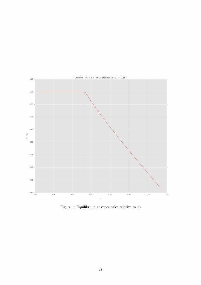
Figure 1: Equilibrium advance sales relative to x∗I

27

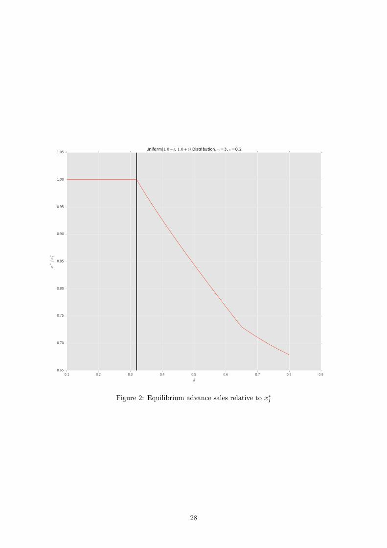
Figure 2: Equilibrium advance sales relative to x∗I

28

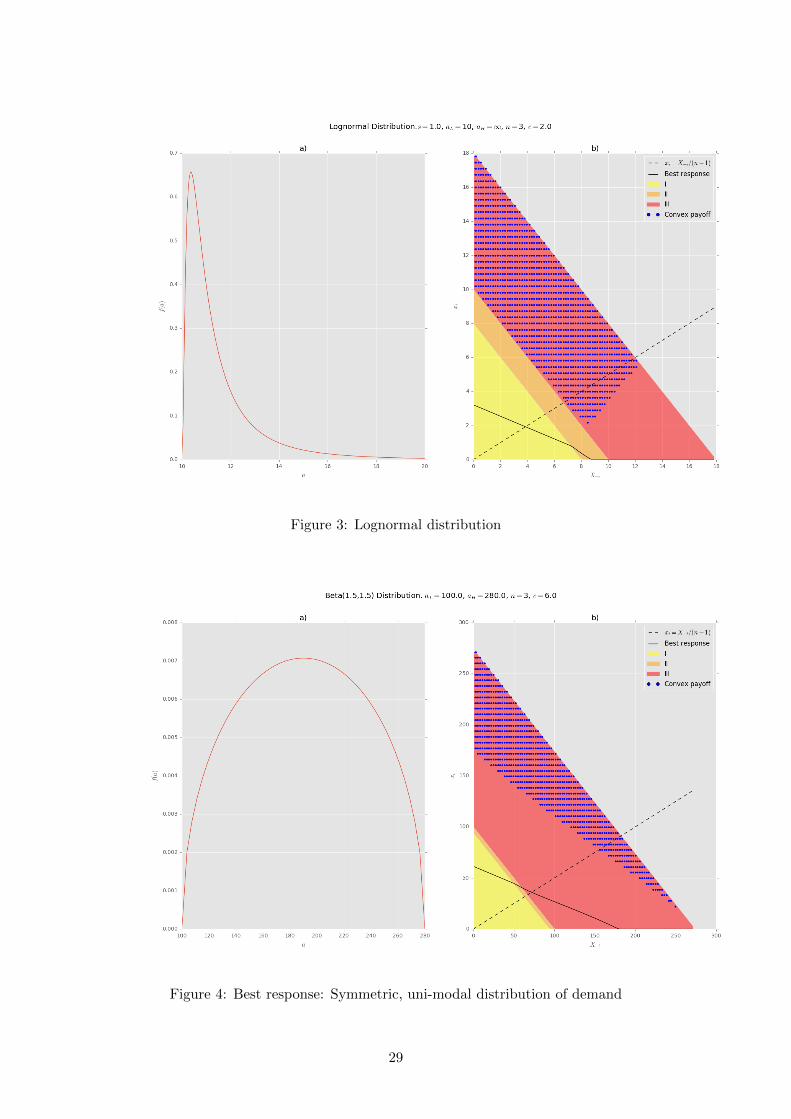
Figure 3: Lognormal distribution

Figure 4: Best response: Symmetric, uni-modal distribution of demand

29

Figure 5: Best response: U-shaped distribution of demand

Figure 6: Bi-modal mixture with modes near together

30

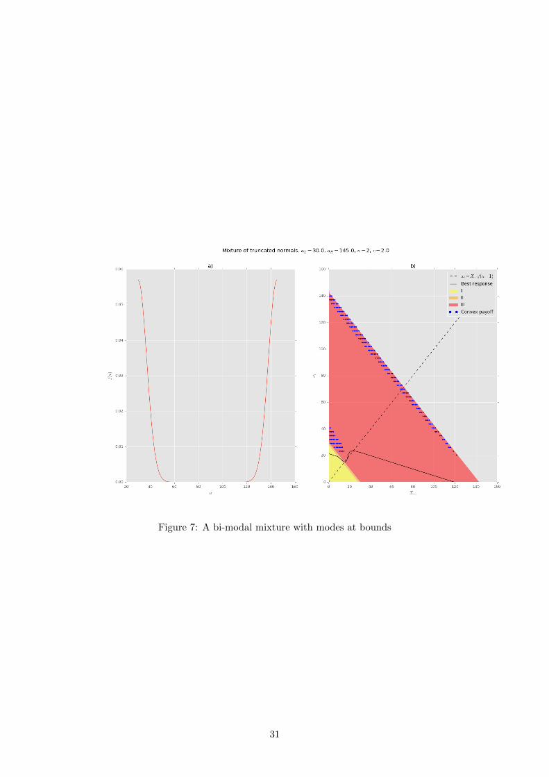
Figure 7: A bi-modal mixture with modes at bounds

31