stratigraphy and heavy mineral analysis in the lower
TRANSCRIPT

W&M ScholarWorks W&M ScholarWorks
Dissertations, Theses, and Masters Projects Theses, Dissertations, & Master Projects
1986
Stratigraphy and heavy mineral analysis in the lower Chesapeake Stratigraphy and heavy mineral analysis in the lower Chesapeake
Bay, Virginia Bay, Virginia
C. R. Berquist Jr College of William and Mary - Virginia Institute of Marine Science
Follow this and additional works at: https://scholarworks.wm.edu/etd
Part of the Paleontology Commons
Recommended Citation Recommended Citation Berquist, C. R. Jr, "Stratigraphy and heavy mineral analysis in the lower Chesapeake Bay, Virginia" (1986). Dissertations, Theses, and Masters Projects. Paper 1539616565. https://dx.doi.org/doi:10.25773/v5-x5k8-kc89
This Dissertation is brought to you for free and open access by the Theses, Dissertations, & Master Projects at W&M ScholarWorks. It has been accepted for inclusion in Dissertations, Theses, and Masters Projects by an authorized administrator of W&M ScholarWorks. For more information, please contact [email protected].

MICROCOPY RESOLUTION TEST CHART NATIONAL BUREAU OF STANDARDS
STANDARD REFERENCE MATERIAL 1010a (ANSI a n d ISO TES T CHART N o. 2)
University Microfilms International A Bell & Howell Information Company
300 N. Zeeb Road, Ann Arbor, Michigan 48106


INFORMATION TO USERS
This reproduction was made from a copy of a manuscript sent to us for publication and microfilming. While the most advanced technology has been used to photograph and reproduce this manuscript, the quality of the reproduction is heavily dependent upon the quality of the material submitted. Pages In any manuscript may have indistinct print. In all cases the best available copy has been filmed.
The following explanation of techniques is provided to help clarify notations which may appear on this reproduction.
1. Manuscripts may not always be complete. When it is not possible to obtain missing pages, a note appears to Indicate this.
2. When copyrighted materials are removed from the manuscript, a note appears to indicate this.
3. Oversize materials (maps, drawings, and charts) are photographed by sectioning the original, beginning at the upper left hand corner and continuing from left to right in equal sections with small overlaps. Each oversize page is also filmed as one exposure and is available, for an additional charge, as a standard 35mm slide or in black and white paper format.*
4. Most photographs reproduce acceptably on positive microfilm or microfiche bu t lack clarity on xerographic copies made from the microfilm. For an additional charge, all photographs are available in black and white standard 35mm slide format.*
*For more information about black and white slides or enlarged paper reproductions, please contact the Dissertations Customer Services Department
A y f T Dissertation IV JL 1 Information Service
University Microfilms InternationalA Bell & Howell Information C om pany3 0 0 N. Z ee b R oad , Ann Arbor, M ichigan 48106


8626063
B erqu is t, Carl R ichard , J r .
STRATIGRAPHY AND HEAVY MINERAL ANALYSIS IN THE LOWER CHESAPEAKE BAY, VIRGINIA
The College of William and Mary in Virginia Ph.D. 1986
UniversityMicrofilms
International 300 N. Zeeb Road, Ann Arbor, Ml 48106
Copyright 1987
by
Berquist, Carl Richard, Jr.
All Rights Reserved


PLEASE NOTE:
In alt cases this material has been filmed in the best possible way from the available copy. Problems encountered with this docum ent have been identified here with a check mark V .
1. Glossy photographs or p ages______
2. Colored illustrations, paper or print _____
3. Photographs with dark background_____
4. illustrations are poor copy______
5. Pages with black marks, not original copy______
6. Print shows through as there is text on both sides of p a g e _______
7. Indistinct, broken o r small print on several pages
8. Print exceeds m argin requirem ents______
9. Tightly bound copy with print lost in sp ine_______
10. Computer printout pages with indistinct print______
11. Page(s)____________ lacking when material received, an d not available from school orauthor.
12. Page(s)____________ seem to b e missing in numbering only as text follows.
13. Two pages num bered . Text follows.
14. Curling and wrinkled pages______
15. Dissertation contains pages with print a t a slant, filmed a s received__________
16. O t h e r __________________________________________________________________
UniversityMicrofilms
International


STRATIGRAPHY AND HEAVY MINERAL ANALYSIS
IN THE
LOWER CHESAPEAKE BAY, VIRGINIA
A DISSERTATION
PRESENTED TO
The Faculty of the School of Marine Science
The College of William and Mary in Virginia
In Partial Fulfillment
Of the Requirements for the Degree of
Doctor of Philosophy
; By
Carl Richard Berquist, Jr.

APPROVAL SHEET
This dissertation is submitted in partial fulfillment of
the requirements for the degree of
Doctor of Philosophy
Carl Richard Berquist, Jr.
Author
Approved, July 1986
Bruce K. Goodwin
Gerald H. Johnson
George- C. Gr^ntDivision of Fisheries and Biological Oceanography

©1987
CARL RICHARD BERQUIST, JR .
All R igh ts R e s e rv e d

TABLE OF CONTENTS
Page
ACKNOWLEDGEMENTS................................................................................ v
LIST OF T A B L E S ............................................................................................. vi
LIST OF FIGURES ........................................................................................... vii
LIST OF APPENDICES.................................................................................... viii
ABSTRACT.......................................................................................................... ix
INTRODUCTION............................................................................................... 1
Setting 1
Rational for this Study 1
Hypotheses 6
Objectives 7
Procedures 7
STRATIGRAPHY............................................................................................... 10
Land 10
Marine 14
FACTOR ANALYSIS........................................................................................ 19
Introduction 19
Pilot Study 22
Explanation of Q-Mode Factor Analysis 28
Q-Mode Procedure as Used in Computer Programs 34
CABFAC Program 34
QMODEL Program 38
EXQMODEL Program 39
iii

HEAVY M INERALS.............................................................................................. 41
Setting 41
Pliocene and Pleistocene Sediments 43
James R iver Sediments 44
Atlantic Shelf a n d Beach 45
Lower C hesapeake Bay 47
Methods 49
Sample C ollection 49
Reduction o f U nw anted Mineral Variation 50
Determ ination o f Mineral Abundance 52
MHS Construction and Separation Principles 55
RESULTS AND DISCUSSION........................................................................... 60
Factor Analysis 60
Procedure 60
Composition P lo ts 62
Other Observations 74
SUMMARY AND CONCLUSIONS.................................................................... 76
APPENDIX A ........................................................................................................... 84
APPENDIX B .............................................................................................................. 91
APPENDIX C ........................................................................................................... 92
APPENDIX D ........................................................................................................... 94
APPENDIX E .........................................I ............................................................... 97
BIBLIOGRAPHY.................................................................................................... 98
V IT A ................................................................ •........................................................ 105
iv

ACKNOWLEDGEMENTS
Sincere appreciation is extended to John D. Boon, III, John M. Zeigler, Bruce K. Goodwin, G. H. Johnson, and George C. G rant for their help and guidance throughout the project and their critical reading of this manuscript. In particular, the author would like to thank John Boon for his assistance in the understanding and use of factor analysis. Appreciation is also extended to Andrew Grosz, Ed Escowitz, and Eric Force of the U.S. Geological Survey, Robert J. Byrne and Adam Frisch of Virginia Institute of Marine Science (VIMS), and Kelvin Ramsey of the University of Delaware for their helpful discussions and comments.
This work would not have been possible without samples provided by Jerry Swean and Ed Meisburger of the U.S. Army Corps of Engineers, Woody Hobbs and Robert Byrne of VIMS, Rich Whitticar and Dan Oyler of Old Dominion U niversity, and data graciously supplied by Frances Firek from her Master’s work at Old Dominion. Steve Skrabal and Chris Mast of VIMS assisted in sample preparation. Additional information was provided by Bob Gammisch and Linda Huzzy of VIMS. Page Herbert of Herbert and Associates, C.J. Carpenter of Carpenter Construction Company, Adli Alliss of Tidewater Construction Company, G.H. Johnson of the College of William and Mary, and Pam Peebles of the Virginia Department of Highways and Transportation supplied subsurface inform ation from boring logs. Adam Frisch, David Evans, Pat Hall, and Bob Lukens cheerfully assisted in the computer analyses at VIMS. Mark Conradi of the William and Mary Physics Department provided explanation of particles in magnetic fields. Appreciation is extended to the William and Mary Geology Department for use of their personal computers, printer, laboratory space and sacrifice of their Frantz separator; Steve Clement provided technical assistance and sample analysis; Mrs. M.E. Magary assisted in the printing and kindly shared her work space. From W.F. Tanner of Florida State University the author received experience rarely found elsewhere in a thoughtful approach to research and synthesis of solutions to problems; although he was not directly involved in this dissertation, his prior association w ith the author was invaluable. The generous support of Bob Milici and Gene Rader of the Virginia Division of Mineral Resources is especially acknowledged; they provided the author with resources and the time to persuc this project.
R.G. Stearns of Vanderbilt University touched o ff the fire of enthusiasm for geology. Alicia and Dick Berquist were supportive throughout the author’s academic progress; their advice to "find excuses to get it done" were heeded. Karen, Peter and Susan Berquist helped with many small but nonetheless im portant tasks as well as provided encouragement and a sense of perspective.
v

LIST OF TABLES
Table Page
1. Correlation chart of pre-Holocene stratigraphic units on the Eastern Shore and southeasternV irg in ia ............................................................................................... 12
2. Average composition of heavy minerals in Pliocene-Pleistocene sediments, southeastern V ir g in ia .......................... 43
3. Average composition of heavy minerals in the JamesRiver estuary ................................................................................... 45
4. Correlation of mean grain size with mineralabundance ........................................................................................ 51
5. Preliminary results of m ineral response in a MHSs e p a ra to r ............................................................................. 59
6. End-members and their compositions of the finalfactor so lu tio n ............................................................................ 61
vi

LIST OF FIGURES
Figure Page
1. Location of study a r e a ........................................................ ................... 2
2. Stratigraphic cross-section across the ChesapeakeBay m o u th ................................................................................................ 5
3. Location of samples, cores and cross-sections.................................. 8
4. Geologic map of study a r e a .................................................. 11
5. N orthern cross-section (A - A’) ............................................................. 15
6. Southern cross-section (B - B ') ............................................................... 16
7. Plot of sample composition loadings on Factor II (pilot s tu d y ). . 26
8. Plot of sample composition loadings on Factor III (pilot s tu d y ) . 27
9. Diagram showing usefulness of Q-mode factor analysis in acomposition problem ............................................................................... 28
10. Example of a hypothetical data m a trix .............................................. 29
11. Diagram showing the concept of rank and factors of a datam a tr ix ......................................................................................................... 30
12. Diagram showing a sample vector plotted in variable and factorsp ace ..................... 33
13. Summary of important minerals from previous studies insoutheastern V irg in ia .......................................................................... 42
14. Example of mineral data sheet and calculation of mineral 'abundance ................................................................................. 54
15. Diagram showing suspension of minerals in a paramagneticsolution w ithin a magnetic f ie ld ....................................................... 56
16. Schematic diagram of the MHS S epara to r......................................... 57
17. Contour map of sample composition loadings on Factor I(combined d a ta ) ..................................................................................... 63
vii

18. Contour map o f sample composition loadings on Factor II (combined d a ta ) ...................................................................................... 64
19. Contour map o f sample composition loadings on Factor III (combined d a ta ) ...................................................................................... 65
20. Isopleth of sample composition loadings for cross-sectionA - A * ....................................................................................................... 67
21. Isopleth of sample composition loadings for cross-sectionB - B’ ....................................................................................................... 68
22. Convergence o f F2 and F3 high concentrations...................... . . 73
LIST OF APPENDICES
PageAPPENDIX A - Core descriptions 84
APPENDIX B - Location and depth of cores 91
APPENDIX C - Sample location in cores 92
APPENDIX D - Sample statistics and composition 94
APPENDIX E - Location and composition of Firek’s samples 97
viii

ABSTRACT
Spatially continuous patterns of heavy m ineral distributions in three
dimensions characterized the sandy Holocene sedim ents of the low er Chesapeake
Bay. A pilot study using Q-mode factor analysis on data from an earlier study
determined m ineral assemblages and mineral composition gradients; the gradients
suggested that surficial sediments entered the Bay from offshore and from older
deposits to the west. Principal components analysis o f the same d a ta indicated that
the abundances o f only S out of 21 minerals were adequate to explain most of the
m ineral variance.
The mineralogy of 87 samples from cores defining two geologic cross-
sections was added to the pilot study data and form ed a new da ta set of 173
samples and S minerals. Q-mode fac to r analysis gave similar end-member composi
tions and mineral gradients as compared to the p ilo t study. M ineral gradients in
the cross-sections show offshore sedim ent rich in amphibole, garnet, and pyroxene
has entered the Bay mouth and presently overlies landw ard-derived sediment rich
in zircon and epidote. The gradients depict tube- an d tongue-shaped pathways lo
cated above paleodrainages. S urficial gradients support the notion of mutually
evasive ebb and flood channels in the Bay entrance. Most of the Holocene sedi
m ent in the lower Bay appears to have originated from outside the Bay mouth, to
include littoral d r i f t from the north. The techniques used in th is study may be
usefu l in an attem pt to subdivide a massive sandy lithosome by recognizing dis
tin c t stratigraphic units of d ifferen t age or origin. A magnetohydrostatic mineral
separator was constructed and tested.

INTRODUCTION
Setting
Southeastern V irginia, including the Chesapeake Bay and the Eastern Shore,
has been the site o f considerable geologic research over the past several years.
This dissertation takes advantage of data generated from some of these earlier
s tu d ie s an d exam ines m inera ls in post-W isconsinan sed im en ts o f th e low er
Chesapeake Bay (Figure 1); also, it is concerned with the stratigraphy, composition
and origin of these sediments through an analysis of m ineral assemblage composi
tion and variability.
Rational for this Study
Recent mapping in the V irginia Coastal Plain (Berquist, Mixon, and Newell,
in preparation; Richmond and others, in press) shows th a t relationships among late
Pliocene and younger formations are complex. Similar processes are responsible
for the deposition of sediments of many of these form ations. For example, the
Windsor, Charles City, Shirley, and Tabb formations (Johnson and Berquist, in
preparation) are all composed of sediments that accum ulated in fluvial, estuarine,
bay, and marine environments. Areas underlain by these units are composed of
juxtaposed, massively bedded sands which commonly are devoid of fossil or dis
tinctive sedim entary structures, and are of d ifferen t ages but sim ilar origin
(depositional environment). Without some contrasting characteristics it is d ifficu lt

2
7 7 7 6 7 5
NEW J E R S E YM A R Y L A N DW. VA.
- 3 9W ashington ,D.C:
DELAWARI
£,<•/
N o r f o lk4 0 miles
5 0 ki lomete rsNORTH CAROLINA
Figure 1. Location of study area in southeastern Virginia.

3
to discrim inate between these similar lithosomes and therefore to map the deposits.
There are several solutions to this problem. M orphologic relationships have
some usefulness in delineating units in the coastal plain. (Coch, 1965; O aks and
Coch, 1973; Peebles, 1984). Absolute soil ages based on 10Be disequilibrium (P avich
and others, 1982) and relative soil ages based on w eathering characteristics
(Mausbach and others, 1982; Owens and others, 1982; and Markewich and others,
1983) are lim ited to surficial units that have developed soil profiles. O ther age-
dating methods may be useful, but only if appropriate carbonate or organic m atte r
is available. F lora or fauna can be used in correlation, but commonly these
materials are e ither leached from the unconsolidated coastal plain sedim ents, or
there is not enough variab ility of the biota to discern between the d iffe ren t fo r
mations. R elative placem ent in a stra tigraphic framework is possible but on ly if
the entire sequence o f a un it or a mappable unconform ity is preserved (Johnson
and others, 1982; Peebles, 1984). The d istribution of heavy minerals (those w ith a
specific gravity greater than 2.8) has also been used to characterize sediments.
V.C. Illing was the first to use heavy minerals for stratigraphic co rre la tion
in 1916; th is m ethod culm inated w ith little advancement in the late 1930’s (Luepke,
1985). M ineralogic correlations fell into disuse because heavy mineral suites were
found to be time-transgressive and other methods of correlation (palynology,
micropaleontology, electric well-Iogs) were found to be m ore sensitive an d con
venient (Van Andel, 1959). Geologists in countries other th an the U.S. con tinued
to use heavy m inerals w ith success (Feo-Codecido, 1956; Luepke, 1985). Van A ndel
(1959) explained th a t this method of research was not worthless and tha t a g rea t
deal of in form ation could be brought out in projects involving location and
characterization o f source regions and sedim ent distribution patterns.

4
Some stratigraphic problems in the Virginia Coastal Plain appear resolvable
by means of a systematic study of heavy minerals. Although contrasting mineral
suites have been generally helpful in the past, identify ing patterns of heavy
mineral distributions may significantly improve the characterization of massive
sands in particular. Distribution patterns or gradients o f mineral compositions
may be unique to d ifferent environments, so contrasting patterns in older sedi
ments could be another means of discerning between otherwise similar lithosomes.
Specifically, Q-mode factor analysis of textural and mineralogic data has been
used successfully to identify unique heavy mineral assemblages and their mixing
gradients (distribution patterns) in modern sediments (Imbrie and Van Andel,
1964; K lovan, 1966; Flores and Shideler, 1978; Rosato and Kulm, 1981; Scheidegger
and Krissek, 1982). Before this method can be used to d ifferentiate between
lithosomes, diagnostic mineral distribution patterns should first be established
within modern analogs.
The Chesapeake Bay, as well as other estuaries, has only recently been
recognized as a center of exceptional sedimentation. The tributary estuaries, erod
ing shorelines, and mainly offshore bottom sediments are probable sources for the
present filling of the Bay (Hobbs and others, 1986); however, the identification of
all the sources and the quantification of sediment from these sources is unknown.
Only one o ther sediment study in the lower Bay begins to address this question;
Fourier grain-shape analysis shows that there is a southerly littoral d rif t of sand
along the Eastern Shore which enters the Bay mouth a t Cape Charles (Boon and
Frisch, 1983). Figure 2 is a stratigraphic cross-section across the Chesapeake Bay
mouth. It is sim ilar to one by Meisburger (1972) but is based on more inform ation
than that available to him. It basically shows th a t sediments in the lower

I
puo(S| euDUJjonsjj
[auuoMO M4J°N
t-
Q . •. in
lauuoqo s[004S diquijm-
. . o
--ir>
a
‘O “OCO
Qou>
_ DcoN
in73C<4^ co
l i■oS2<*- « C*-,-O JJ
. G pqCO coL1 V.g 42tJ 3, g «u «° 6 Uh fi
x8 o Z «
? s3 nC/5
« « ■° rve a3 -a <; a| SS 'Sa cis s3 d a**•* 5i corT *nI s * 0 6 -oIh h£ « Pm co
X 25 S « « g-aco » 2r w w o 3 3 3
COo£ C/5S Z Z O 'T S
zoHHH<Z- ICl,
Xw
« 0 to G G
a c / a
•o3Eu
C/5 «3 3
pm rtO 8 u t> s es u o o o o oo o X X
O to
ee* t!00 3 b. uo a u u a c u o u o o oo o X X
B no o.
TJgrtCOo fe.5 >£ °H-l
« S ? w3 TJ g a” 3.S’ L-C5 O*3 *pH wa 8 o «
•pp b-
3 o
o U [u oW T3 CD3 3 3S *3.2 2 .2 « U. >» P£ s<2
>•H
x>36>5
XI33C/13OC4BLaOHa3U>3.338>.
hJ
XI33
O 'j*3O>>
• HCO■ S’o cd
co *7tO '7. os &.2 3 5 00 3 J;e °L- *3o apH 32 3 o o► H Q ,
O 1oo JJ •a °*« # co O '
~-4 COO' O'
Figu
re
2. Cr
oss-
sect
ion
along
the
C
hesa
peak
e Ba
y Br
idge
T
unne
l

6
Chesapeake Bay are composed m ainly of massive post-Wisconsinan sands overlying
T ertiary strata and th a t much of the Pleistocene sedim ent has been eroded during
preceeding lowstands o f sea level.
Q u a te rn a ry sed im en ts in th e V irg in ia C o a s ta l P lain w ere deposited
prim arily during m arine transgressions (Johnson an d others, 1982) an d are there
fore similar to the post-Wisconsinan Chesapeake Bay sediments in term s of a
depositional model. I f Q-mode fac to r analysis is app lied to the heavy m ineral data
in the post-Wisconsinan sand lithosom e of the lower Bay, these patterns resulting
from contoured plots o f sample composition loadings on end-members theoretically
should reflect transgressive (marine) sedimentation an d the influx of sand into the
Bay from offshore and other "sources"; although absolute sources o f sediment
would not be known, transport directions may be im plied by m ixing gradients.
Some mineral d istribu tion patterns m ight then be established for the m outh of a
modern estuary .
Hypotheses
Two hypotheses guided this research. The f i r s t is that heavy m inerals exist
in the post-Wisconsinan Bay sands, and that these m inerals and their distributions
can be used to characterize patterns and features otherw ise impossible to distin
guish within this massive sand lithosome. The second hypothesis is th a t patterns or
gradients of m ineral compositions defined by Q-mode factor analysis should
reflect the advection o f sand into the Chesapeake Bay mouth from offshore and
from other sources during the post-Wisconsinan transgression. T herefore , in the
Bay entrance area, fluv ial deposits th a t originated landw ard should generally be

found below sands th a t originated on the shelf if the post-Wisconsinan sedim ents
were deposited during a marine transgression.
Objectives
The purpose o f th is research is to characterize post-Wisconsinan sands of
the lower Chesapeake Bay based on heavy mineral compositions by establishing
mineral patterns or composition gradients in three dimensions. These patterns
should re flec t real processes and indicate sediment transport directions. This in
form ation should substiantiate some prior notions of the origin of sedim ents
deposited in an estuarine environment and hopefully provide a basis for fu tu re
comparison of massively-bedded sands.
Procedures
In order to accomplish these goals, the stratigraphy of the lower Bay (in
three cross-sections) and the surrounding land area was established using published
and unpublished or new core and seismic data. F ifteen cores were selected and
defined two cross-sections oriented approximately east-west and out of the Bay
mouth (F igure 3). At least six samples were taken from each core; textural analysis
was achieved by sieving. Heavy minerals were separated from the 3 to 4 Phi size
range by means of a heavy liquid (tetrabromoethane). Samples were subdivided
into six groups using the Frantz Isodynamic separator and mineral compositions
were determ ined under a binocular microscope. Q-mode factor analysis was used
to establish unique heavy mineral suites and d istribution gradients for the post-

8
Figu
re
3.Lo
catio
n of
cros
s-sc
ctio
ns,
core
s us
ed
in th
is st
udy,
and
Fi
rck’
s gr
ab
sam
ples
in
the
low
er
Che
sape
ake
Bay.

9
Wisconsinan sediments in each cross-section. The procedure for acquiring mineral
compositions was compatable with the work of Firek (1975) so that both her data
and the data from this study could be combined. In this dissertation, the following
chapters contain more detailed procedures used to obtain data.

STRATIGRAPHY
Land
Many individuals studied the geology in the lower Bay area beginning with
W.B. Rodgers in 1835. Subsequent work was summarized by Oaks and Dubar
(1974) and Peebles (1984). Much of the present geologic knowledge of southeastern
Virginia evolved from Oaks and Coch (1973); however, th e ir stratigraphic
framework was amended by more recent detailed and regional mapping. In the
Hampton-Newport News area, Johnson (1976) recognized regional unconformities
in previously mapped facies of the Norfolk Formation. He clarified stratigraphic
relationships on the York-James Peninsula and named the Tabb Formation with
three members, Sedgefield, Lynnhaven, and Poquoson. These units did not corre
late clearly w ith the stratigraphy defined by Oaks and Coch (1973) south of the
James River. Additional work by Peebles (1984) and Peebles and others (1984)
simplified the regional stratigraphy and resolved correlation problems across the
James River.
Richm ond and others (1986) mapped the Q uaternary deposits of this area
without using formal stratigraphic names. This dissertation relied upon a similar
p ro jec t o f com pila tion and m apping by B erq u ist, M ixon and Newell (in
preparation); their report used formalized geologic names (Figure 4) and the mem
bers of the Tabb Formation were elevated in rank to formations. Both of these
regional maps showed comparable distributions of Quaternary sediments, but d if
fered in detail because of the published scale and mapping units.
10

Cap
*
11

12
Mixon (1985) published a geologic map of the Eastern Shore and sum
m arized absolute ages fo r the coastal p lain area (Mixon and others, 1982). The
stratigraphic nom enclature in Delaware and M aryland (Owens and Denny, 1979)
was continued w ith some m odifications into the V irginia Eastern Shore; fo r this
reason, the nom enclature on the Eastern Shore is d iffe ren t from the rest of
V irginia. Table 1 summarizes the present knowledge o f stratigraphic relationships
w ithin the boundaries o f this dissertation. Some correlation problems between the
Delmarva Peninsula and the rest of V irginia remain to be solved.
TABLE 1
Correlation ch art of pre-Holocene stratigraphic units on the EasternShore and southeastern V irginia.
In this study area Eastern Shoreonly (Mixon, 1985)
Sedgefield Form ation S tum ptow n a n d B u tle r’s B lu f fMembers, Nassawadox Formation
Lynnhaven Form ation Joynes Neck Sand and part o f Oc-cohannock M em ber, N assaw adox Formation
Poquoson Form ation Wachapreague Formation
These form ations (Table 1) are composed of sedim ents deposited during the
Sangamon Interglaciation. The older units (Lynnhaven and Sedgefield and their
equivalents) were form ed during m arine transgressions. Uranium-series dates from
correlative deposits ranged from 51,000 to 101,000 years; correlation w ith these

13
dates was determ ined by a ttribu ting Mixon's samples (Mixon and others, 1982) not
to the formations he used but to units (Sedgefield, Lynnhaven, and Poquoson
formations) from unpublished mapping by Johnson and Berquist. The Poquoson -
Wachapreague deposits were form ed during a m arine regression prio r to the Wis-
consinan (Johnson, 1976; Leonard, 1986). Estimates of absolute ages for the
Wachapreague Formation range from 128,000 to 82,000 years B.P. (Mixon, 1985).
Sediments composing these late Pleistocene formations are variable in com
position because many depositional environments are represented in each unit. In
actuality, the Pleistocene units are alloformations because they are usually
bounded by unconformities (N orth American Stratigraphic Code, 1983); however,
this report will continue to use "formation" in terminology.
Stratigraphic mapping and correlation done for the V irginia Division of
Mineral Resources is based predominantly upon lithofogic criteria. However, for
mation boundaries are not placed, for example, between any sand and clay
lithosome. A logical and very workable subdivision of coastal p lain sediments is
one based on an expected succession of environments (deposits) which occur during
a major marine transgression or regression and is discussed by Peebles (1984). In
addition, there is a consistent relationship of the surficial sediments to morphology
(topographic expression) of the stratigraphic units throughout the region. For
example, sandy barrier deposits o f the Sedgefield Formation are a t the same eleva
tion as sandy barrier sediments of the Butlers B luff Member o f the Nassawadox
Formation; muddy estuarine and back-barrier deposits of these two units are also
a t the same position relative to sea-level. Furthermore, the stratigraphic position
of these units is comparable: they are both inset against older stratigraphic units;

14
the older units share the same sediment-morphologic relationships (but a t a higher
elevation) as the Sedgefield-Butlers B lu ff deposits. T hus, regional stratigraphic
correlation of coastal plain stratigraphic un its is dependent upon the determina
tion o f several c rite ria .
Marine
Figure 2 is a cross-section which is sim ilar to th a t o f Meisburger (1972) and
M oran and others (1960); there are two reasons for d ifferences between Figure 2
and the earlier sections. First, the s tra tig rap h y on land is now more thoroughly
known, and second, I have re-interpreted la teral continuity of sediments between
borings based on an expected succession of environm ents during a marine
transgression.
Figure 2 shows that the muddy sedim ents of the Lynnhaven Form ation are
less than 5 feet th ick and contrast to the coarse sands of the underlying Sedgefield
Form ation. S im ilar relationships are fo u n d on the southern tip o f the Eastern
Shore where thin an d muddy Joynes N eck deposits overlie the sandy Occohannock
sediments. C orrelation is guided by superposition o f sequences o f material
(determ ined by hand augering) and by th e subtle but very consistent morphology
around the shores o f the Bay.
Figures 5 an d 6 are two geologic cross-sections jo in ing the cores used in this
study. The indicated post-W isconsinan-Tertiary contact between cores is based on
seismic data an d /o r additional cores fro m Meisburger (1972), Byrne an d others
(1982), and Carron (1979). Descriptions o f the core sedim ents are in A ppendix A.

15
CERC 26
CERC 55
Nautilus Shoal
CERC 9
CERC 11 CBBT
Cross-section
Chesapeake Channel
WB072
to
WB082
WB101
WB063inCM ’Om
IIcu■o's£ii
s13CCSUiIt
C/3
OuaoBCJnTJC«cn00cU>O■O6o
c?rf
<t<G
,240 uin1ininOwOoi H00ooo00
uU W u Xs t:
.2? O LLi Z pe
at,
T =
Terti
ary
sedi
men
ts.

16
iip.
CD
CD
VC10J
WB081
WB062
WB095
WB092
Thimbl« Shoals Channel ao
COin
WB098
WB101 LTlO
■o3Sii
s
•oacacotl
C/3
too(Mu.oua.a• H£CO5CO•acCTJto00at-oX3So
c?COu,•a03I
mco4-o0 co1COCOOuUCJ*5)ooooo
« so u 00 3
OU* c/J pe
at,
T =
Terti
ary
sedi
men
ts.

17
The coordinates and water depths of the cores are given in Appendix B.
The post-Wisconsinan age o f the sediments overlying the T ertiary deposits
as shown in cross-sections of Figures 2, 5, and 6 can be demonstrated by relying
upon absolute ages and by tracing repetitive sequences of sediments la terally from
borings. Carbon-14 dates on peat in boring M-28 define ages of 10,340 -+ 130 and
15,280 -+200 years B.P. a t respective depths of 82 and 89 feet below mean low
water; other younger dates are also reported (H arrison and others, 1965).
Consequently, the overlying sands are of post-Wisconsinan age. In areas where no
ages have been determ ined and lateral continuity of organic deposits cannot be
shown, a de fin ite age is less certain; however, correlation can be based on a similar
vertical arrangem ent of sediments. Nearly all paleochannels in the lower Bay con
tain sediments th a t show a m arine transgressive sequence; this is from bottom to
top, a lag gravel (fluvial), organics (fluvial to estuarine), muds (estuarine), and
sand (bay-m outh to marine). For example, the sediments in the buried channel un
der Fisherm ans Island are not dated, but are probably post-Wisconsinan based on
continuity of the upper sand and a similar sequence to the region of boring M-28.
O ther areas in the Bay may show a d ifferen t vertical sequence because the succes
sion of environm ents at those locations during the transgression is variable, as
supported by K ra ft (1971).
Several c rite ria allow fo r recognition of the Pliocene Yorktown Formation.
McLean (1966) shows a Tertiary-Q uaternary contact based on lithologic and faunal
changes in the Chesapeake Bay Bridge-Tunnel cores. The same contact is evident
in seismic reflection and core data from Meisburger (1972) and Byrne and others
(1982). Engineering data from Moran and others (1960) is also helpful as

18
Yorktown sediments are commonly over-consolidated (very high penetration blow-
counts). Sediments of the Pliocene Chowan R iver Formation are identified below
Cape Henry (Oyler, 1984). These deposits overlying the Y orktown occur sporadi
cally in the V irginia Beach area and are not delineated in this study.
Having defined the stratigraphy in the study area, the location of the post-
Wisconsinan deposits relative to older stratigraphic units is established. This is
im portant fo r two reasons. First, possible sources of sediment to the Bay from
land are indicated. Second, the origin of samples taken fo r mineral analysis
should not be questionable. I f samples were unknowingly selected from Pleis
tocene or T ertiary deposits, the interpretation o f mineral gradients from the post-
Wisconsinan deposits could be erroneous.

FACTOR ANALYSIS
Introduction
A lthough originally applied in psychological studies, factor analysis has
recently been used for gaining greater insight into solutions of geologic problems.
When the num ber of variables and /or samples becomes large, in terpreta tion of data
by inspection is d ifficu lt or impossible. Factor analysis provides an objective solu
tion to the problem of sim plifying and explaining large amounts o f m ultivariate
data. In th is research, the variables are the weight percent of up to 18 minerals
observed on 277 samples in the lower Chesapeake Bay.
T he methods described later in this chapter may be in troduced w ith a
geometric presentation. A "variable space" may be created where each coordinate
axis represents the abundance of a particular mineral. Samples plotted in this
space m ay be compared w ith each other in terms of their sim ilarity or dis
sim ilarity. Conversely, each observation can be used to define a "sample space" in
which one variable is compared to one another. A close grouping in space signifies
a close or common relationship. The goal o f these m ultivariate procedures is to a r
rive w ith few er but more m eaningful variables which are com binations of the
original ones.
R-m ode factor analysis is concerned with the groupings and relationships of
variables. F irek (1975) and Firek and others (1977) used one-way analysis of
19

20
variance between pairs o f a rb itrarily defined provinces and R-mode factor
analysis on a data base o f heavy m ineral compositions obtained from bottom grab
samples in the lower Chesapeake Bay. Firek determ ined five mineral suites for
each of her five provinces. Two facto rs were used in her analysis and cor
responded to two m ineral suites; she believed that sedim ent maturity was respon
sible fo r the grouping o f minerals in one suite while provenance accounted fo r the
association of minerals in the other suite. Based on the way minerals com pared be
tween the provinces in the Bay and the combination o f minerals composing each
fac to r, she believed th a t her study supported the notion of sediment transport into
the bay from offshore as well as from erosion of surrounding land.
Q-mode factor analysis establishes the relationships between samples. Pre
vious studies involving compositional d a ta from spatially distributed samples have
benefitted in particular from Q-mode fac to r analysis. The first geological applica
tion of this method was m ade by Im brie and Purdy (1962) where they defined five
sample groups (oolite, oolitic, grapestone, coralgal, and lime mud) as a basis for
classification of carbonate sediments. Imbrie and Van Andel (1964) compared
conventional comparison methods w ith Q-mode factor analysis (vector) techniques
in heavy-mineral province studies. In the Gulf of California they found that
characteristic mineral assemblages were clearly defined by inspection o f the data
and tha t mixing during sedim ent transport was minimal; there was also a clear
relationship between sources of mineral suites and the calculated end-members or
factors. However, on the Orinoco-Guayana Shelf o ff the north coast of South
America, mixing of sedim ent was common and sources and mineral assemblages

21
were complex. They found that vector patterns were much more meaningful than
conventional inspection of the data; the interpretation of fac to r plots suggested
that submerged Pleistocene shorelines and ancient littoral d r if t could have been
responsible for the distribution o f observed heavy minerals.
Klovan (1966) a ttributed the grain size distribution o f sediments to a
hydraulic energy regime. His study showed that sediments from Barataria Bay on
the southeast coast of Louisiana could be subdivided into three groups (factors)
through vector analysis; plotting the samples (as vectors in fac to r space) on a map
indicated that three regimes characterized by their relative energies (surf, current
or gravitational settling) were responsible for trends in the grain size distributions.
Constant row-sums of compositional data pose no problem in Q-mode
analysis. Miesch (1976) took advantage of this fac t and modified the Klovan and
Imbrie (1971) routine to reproduce approximations of the observed data in similar
units (weight percent or parts per million, etc.). The earlier method reproduced the
original data in a normalized form, so the later improvement gave the user an ad
ditional means of critizing factor analysis results for geologic reality . Miesch
(1976) also demonstrated the usefulness of this modification in geochemical and
petrologic mixing problems.
Flores and Shideler (1978) used Q-mode factor analysis to define three
suites of heavy minerals in the Texas Gulf of Mexico w hich were: opaque-
pyroxene-garnet from the ancestral Rio Grande delta; tourm aline-green hornblende
from the ancestral Brazos-Colorado delta; and a mixed suite from both regions.
Variation of the minerals w ithin each factor-defined province was thought to be

22
caused by hydraulic fractionation and selective chemical decomposition.
Perhaps the most powerful attribute of the Q-mode method is its ability to
simplify real but complex compositional data. Q-mode factor analysis has been
used to describe a collection of samples not in terms of many original variables but
as a mixture of a few theoretical or real "end-member" samples. The samples
usually represent compositional extremes for the data set. The routine indicates
how much of each end-member is present in all samples. Because the dimen
sionality of the original data is reduced, composition gradients o f a suite of
minerals (based on the amount of an end-member in each sample) can be shown on
a map; these patterns can suggest a direction of sedim ent transport sim ilar to the
results of using tracer sediments (Imbrie and Van Andel, 1964; Flores and Shideler,
1978).
In summary, the use of factor analysis results in objectively defined groups
of samples which may not be apparent from conventional inspection of the data, as
shown by the Orinoco-Guayana Shelf study (Imbrie and Van Andel, 1964). New or
d ifferen t associations of data may result from a factor analysis model and there
fore may require a reasonable geologic explanation. This added insight gained
from the analysis provides increased clarification of otherwise enigmatically re
lated data.
Pilot study
In order to establish the validity of the proposed approach, Q-mode factor

23
analysis programs developed by Klovan and Im brie (1971), K lovan and Miesch
(1975) and Full and others (1981), were applied to F irek’s original data. The loca
tion and tabulation o f all her data may be found in her thesis (Firek, 1975); Figure
3 and Appendix E only gives the data that I used in my final analysis. Firek iden
tif ied 21 minerals (plus "other") b u t olivene, topaz, and zoisite were reported as ab
sent or as non-num eric (trace) amounts; these m inerals were therefore excluded
from all of my work. I then incorporated her data into several fac to r analysis
models. First, all data were used (190 samples and 19 variables, or 18 minerals plus
"unidentified") in three, four, fiv e and six factor models. The three fac to r solution
provided the most geologically reasonable model because end-members uniquely
coincided w ith th ree o f Firek’s provinces. Solutions using additional factors par
tia lly duplicated the end-member suite of m inerals and their locations in the
provinces of the th ree factor solution. Plots of the composition loadings of
samples on end-members showed geologically reasonable patterns; the gradient of
garnet-hornblende composition decreased in the up-Bay direction and was consis
tent w ith sand advection into the Bay mouth from offshore; the gradient of
clinopyroxene-hornblende opposed the first plot and probably represented the con
tribu tion of sedim ent from rivers or shoreline erosion; the th ird plot showed
mixing of both factors. U nfortunately, the end-members were characterized by
large negative m ineral percentages, so a more realistic solution was sought.
Next, I in troduced Firek’s d a ta to a principal component analysis using the
programs from Davis (1973); it was determined th a t seven minerals (hornblende,
zircon, garnet, clinopyroxene, sphene, epidote, and staurolite) out of the original

24
18 accounted for 96% of the variance in the entire data set. Then, using only eight
variables (seven minerals and one "other", recalculated to constant row-sums of
100%) and 190 samples, several factor solutions were attempted w ith similar results
which were duplication of provinces and negative end-member compositions. Be
cause the sampled area was so large, there could have been more than six extreme
samples (or end-members); the spread or diversity of the data might have required
greater than six factors for a reasonable solution. Another analytical approach
gave more understandable results. The geographic size of the study area was
reduced and only 87 samples (location shown in Figure 3) from the lower Bay area
were used; also, the samples (each composed o f seven minerals) were row-
normalized. A three factor solution gave large negative values of end-member
compositions, but accounted for 97% of the total variance; a four factor solution
gave more reasonable results because end-member compositions were essentially
positive. Two of the four factor plots were not easily explainable; one suggested a
western source of material to the Bay that was rich in staurolite, while the other
plot showed high concentrations of amphibole-rich material around the margins of
the lower Bay. The other plots of sample composition loadings were similar to two
of those from the 3 factor solution. These results reflected the complex currents
and zig-zag shoals shown by Ludwick's (1970) studies, and the diverse sediment
sources in the lower Bay area.
Figure 7 showing the distribution of Factor 2 very clearly depicts the in
flux of sediment into the Bay mouth from offshore. The end-member is located
o ff Cape Charles and is composed of 27% amphibole and 72% garnet; this composi

25
tion is sim ilar to mineral compositions on N orth Carolina beaches and dunes (Giles
and Pilkey, 1965). The offshore source is also predicted by littoral d r if t conver
gence at the Bay mouth (Swift and others, 1972; Firek and others, 1977; Harrison
and others, 1967).
The existance of a zircon-rich region through the center of the lower Bay
(Figure 8) w arrants fu rther study partly because heavy m ineral data from the sur
rounding land and tribu tary estuaries is lacking. The h igh zircon composition
w ith associated sphene, epidote, and stauro lite suggests th a t a combination of
moderately young m aterial and much older sediments are being reworked by
modern processes. Zircon is a more stable m ineral and is more commonly found in
older sediments while the other minerals are less stable and a re commonly found in
younger sedim ents (Pettijohn, 1957). Because o f duplicated patterns in a three and
four factor solution with d iffe ren t data sets, it is strongly believed th a t these
gradients of m ineral compositions suggest the pathways o f sedim ent transport in
the lower Bay area.

I
Figu
re
7.C
onto
ur
map
of sa
mpl
e co
mpo
sitio
n lo
adin
gs
on a
fact
or
com
pose
d of
72%
garn
et
and
27%
amph
ibol
c;
sam
ple
mar
ked
"Fac
tor
2" wa
s ch
osed
by
the
Q-M
ODEL
pr
ogra
m
as an
end-
mem
ber
from
Fire
k’s
data
only
.

a
U J CO
UJ CO-1 U J o
01 CMCO CM
N CO
27
•g 6§ eO t-i
2 aQ . O° 6 ■m"0 C Cg «•** c a c5w incT w
8 Iin r t
n e o o
*-•O O. n hJ§gO io o '
u *"<2 >* J3w C _ oQ in0 O Xin o M - c « n2 * CM2 f r >
c *H1 23 ga '6 73 o « o as« rt SB a sctf03 O ,
aCm CO O co
CO M 6 . .
>> Ma oCO ♦-»
o 43O O l,"13o 33 05 ."S 2 2 m3 h 3 O.» S 3 .sU-c CJ to Uh
28
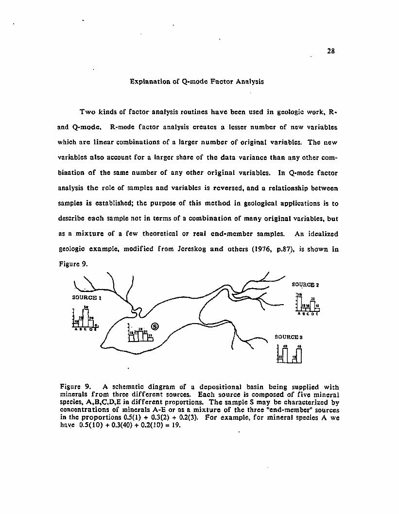
Explanation of Q-mode F ac to r Analysis
T w o kinds of factor analysis routines have been used in geologic work, R-
and Q-mode. R-mode factor analysis creates a lesser num ber of new variables
which a re linear combinations of a larger num ber of original variables. The new
variables a lso account fo r a larger share of the d a ta variance than any other com
bination o f the same number of any other o rig inal variables. In Q-mode factor
analysis th e role of samples and variables is reversed, and a relationship between
samples is established; the purpose of this m ethod in geological applications is to
describe each sample not in terms of a com bination of many original variables, but
as a m ix tu re of a few theoretical or real end-m em ber samples. An idealized
geologic exam ple, modified from Joreskog an d others (1976, p.87), is shown in
Figure 9.
SOURCE 2■ <•
SOURCE 1It mol
»
SOURCES
Figure 9. A schematic diagram of a depositional basin being supplied w ith minerals fro m three d iffe ren t sources. Each source is composed of five mineral species, A,B,C,D,E in d ifferen t proportions. T he sample S may be characterized by concentrations of minerals A-E or as a m ixture of the three "end-member" sources in the proportions 0.5(1) + 0.3(2) + 0.2(3). For example, for m ineral species A we have 0.5(10) + 0.3(40) + 0.2(10) = 19.

29
As minerals arrive in the basin (Figure 9) from each o f the source rivers,
they are mixed into new proportions. If this were an ancient system and we were
relying on core data, and our objective was to find the sources o f the minerals, we
would not know how many sources there were and it would be very d ifficu lt to
solve th is problem by mere inspection of the mineral compositions. Q-mode facto r
analysis has the potential of finding the end-members and their compositions and
"un-mixing" all the samples in terms of the end-members.
A lthough Davis (1973, 1986) and Joreskog and others (1976) present a
detailed explanation of the method, an abbreviated description o f this process w ill
be explained here. We should first arrange our data into a m atrix form at where
each row represents a d ifferen t sample and each column is a d iffe ren t variable
(Figure 10).
sample garnet hornblende zircon ...k
si 15% 25% 60%s2 8% 11% 21%
r
Figure 10. Data matrix C, with r rows o f samples and k columns of variables.
This data m atrix C can be approxim ated or factored into two other matrices
of lesser rank where "the rank of a m atrix is the smallest common order among all
pairs of matrices whose product is the m atrix" (Joreskog and others, 1976, p. 36).

30
M atrix C can actually be decomposed into an in fin ite number o f product matrices
A and B (Joreskog and others, 1976, p. 35); combinations involving matrices of
three d iffe ren t ranks are shown in Figure 11. M atrix m ultiplication requires tha t
the number o f columns (m) in the pre-factor (A) must equal the number of rows
(m) in the post-factor (B).
m
m BTTT
E Erri k
r rA c
Figure 11. The number of rows (r) and columns (k) of the m atrices are drawn to scale. The ran k of C is m in each example; m is also the num ber of factors th a t could be chosen for any particu lar solution.
H aving an infinite num ber o f choices o f product matrices does not provide
any help in sim plifying the d a ta matrix. We can limit our choices by asking th a t
the new m atrices will fu lfill certain additional requirements. At this point in the
discussion, eigenvectors, eigenvalues and the Eckart-Young theorem will be in tro
duced.
It is d iff icu lt to define eigenvalues and eigenvectors w ithout a lengthy dis-

31
cussion (see Davis, 1973 and Joreskog and others, 1976 for more detail). For this
discussion I will use a few simple examples. A m atrix can be geometrically repre
sented as vectors in multidimensional space. Each vector is defined by a row in
the m atrix where row values are the coordinates o f the vector end-point. For ex
ample, sample SI of Figure 10 is plotted in Figure 12 A. The values of a sym
metric m atrix (2 x 2) may be shown to plot on an ellipse (in 2 dimensional space).
The eigenvectors of this m atrix are the major and minor axes of the ellipse; the
eigenvalues are the lengths o f each axis. The eigenvectors are perpendicular
(orthogonal) to each other and each one has an associated eigenvalue. Being or
thogonal means that the vectors are independent of one another. A symmetric
m atrix will always have real as opposed to imaginary eigenvalues; this fact is im
portant because the original data matrix is converted to a symmetric matrix in R-
and Q-mode factor anlysis routines. The rank of a m atrix is also equivalent to the
number of its non-zero eigenvalues.
The Eckart-Young theorem states (after rearranging the matrices) that any
real m atrix [CJ equals [V][N][U]’ where [V] and [U] are orthogonal matrices and [N]
is a diagonal m atrix containing the eigenvalues of [R] or [Q] described below. (U*
means the transpose of U). The minor product m atrix [R] = [C][C]’ and the
columns of [U] contain the eigenvectors of [RJ. Likewise, the major product
matrix [Q] equals [C]’[C] and the columns of [VJ contain the eigenvectors of [Q]
(Davis, 1986, p. 517 - 519). Without going into more detail, it may be shown that
[V][N] becomes the factor loadings matrix (matrix A in Figure 11) and [U] becomes
the factor scores matrix (matrix B in Figure II).

In Q-mode facto r analysis, the da ta matrix is factored into A, the factor
loadings m atrix (which gives the composition of each sample in term s of the
factors) and B, the facto r scores m atrix (which describes the composition of each
factor in terms of the original variables and may be used to convert new data into
"factor space". The investigator may choose the num ber o f factors (which will of
ten be less than the rank of the transform ed data m atrix) based on crite ria ex
plained later.
Finding the eigenvalues and eigenvectors o f a variance-covariance matrix
or sim ilarity m atrix (derived from the original da ta matrix) has special sig
n ificance to understanding the structure o f the original data. The to tal variance
o f the data is equal to the sum of the eigenvalues of the variance-covariance or
sim ilarity matrix. Thus the choice in the number of factors is directly related to
the amount of variance in the data to be retained and explained.
It would be helpful to the understanding of this type of analysis i f we can
visualize each sample as a vector which is plotted in variable space, th a t is, within
a coordinate system where each axis is a variable. For more than three variables it
is d ifficu lt to see how this can be done, so a simple example is shown in Figure 12.
Through Q-mode factor analysis, we may find th a t the contribution of gar
net (Figure 12) to the total variance in this geologic data is very small (for most
samples, garnet composition may remain nearly the same or vary only slightly) and
we could sim plify the relationship of samples to one another by reducing the
dimensions of the data. In Figure 12 a three-variable data matrix is reduced to a
tw o-factor matrix. Through the analysis, garnet composition is combined with

33
ano ther variable in defining a fac to r; alternately garnet composition could be
elim inated , particu larly if its abundance varies only slightly. The composition of
the sample is changed relative to the new factor coordinates. Each new ax is or
fa c to r has a composition in terms o f orig inal variables and can be an actual sam ple
from the data m atrix . The value o f th is approach can be appreciated w hen the
analysis reduces a ten-variable system to a three or four facto r model.
2 -
4-
0
S = 15% gamtt35% hombtmd*60% clrcon
2
S
S' — 30% factor 170% factor 2
4 0 2 4A B
F ig u re 12. Sample S plotted in v ariab le space (A) and fac to r space (B). F a c to r 1 m ay be composed predominantly o f hornblende or a com bination of hornblende and garnet. Factor 2 may be composed m ainly o f zircon.

34
Q-mode Procedure as Used in Computer Programs
M ineral composition data was used in three computer programs, CABFAC
(Klovan and Imbrie, 1971), QMODEL (Klovan and Miesch, 1975), and EXQMODEL
(Full and others, 1981). The Q-mode factor analysis method is explained as the
programs derive a fina l result.
CABFAC Program
Depending on the type of data, some transform ation may be needed (Davis,
1973; Miesch, 1976). Several options are available in the program to scale columns
of variables. The reason fo r scaling is to give all variables an equal weight in the
factor analysis.
A ll factor routines begin with the calculation of a square "similarity"
matrix w hich may be the correlation coefficients or some other measure of
similarity th a t does not exceed the range of -+1.0. The correlation coefficient, (r,
and thus R-mode) is not used as a measure of sim ilarity between samples (in Q-
mode) because it requires the calculation of variance across variables; averaging
the amount of each variable in a sample is an obscure procedure (Davis, 1973, p.
526). Im brie and Purdy (1962) defined an "index of proportional similarity" or
cosine T heta which is the cosine of the angle between two row vectors plotted in

35
variable space. If two samples are plotted orthogonal to each other, Theta = 90°
and cosine Theta = 0 so it can be said that the two samples have no similarity. If
two samples are co-linear, Theta = 0° and cosine Theta = 1 and it is obvious that
the samples are identical. This concept is d ifficu lt to visualize beyond three
dimensional (variable) space, but the mathematical calculations of cosine Theta in
hyperspace is not affected by our lack of perception. CABFAC computes a cosine
Theta m atrix from the data which will be symmetric in all cases.
The next step requires calculation of the principal components or eigenvec
tors and eigenvalues o f the cosine Theta matrix. Davis (1973) explains the utility
of eigenvectors and how they are calculated, so only a few important facts are
summarized here. The sim ilarity m atrix is symmetric so the eigenvalues will be
real, and the eigenvectors will be a t right angles to each other, or orthogonal. For
example, the values of a 2 X 2 symmetric m atrix can be shown to represent coor
dinates o f points in two dimensional space. The points lie on the boundary of an
ellipse whose center is the origin of the coordinate system. The eigenvalues are the
lengths o f the major and minor axes of the ellipse; each eigenvalue has an as
sociated eigenvector th a t is the slope of each ellipse axis. In addition, the sum of
the eigenvalues equals the sum of the diagonal elements or trace of the sim ilarity
matrix. These facts are important when applied to the sim ilarity matrix because
they describe some major characteristics of the original data. The trace of the
sim ilarity matrix also represents the variance in the original data matrix; so each
eigenvalue then represents a portion of the total variance. CABFAC converts a
normalized eigenvector to a factor by multiplying every element of the eigenvector

36
by the square root o f the corresponding eigenvalue. In other words, the o rien ta
tion of the factors are the same as the eigenvectors. The "factors" in fac to r
analysis are then eigenvectors that are weighted proportionally to the am ount of
total variance which it represents. These weightings of the eigenvector are called
factor loadings. CABFAC calculates and lists the eigenvalues and th e ir cumulative
variance so one has the means of choosing how much variance he would like to ex
plain and therefore how many factors will be needed; a three factor solution
would more simply explain the data but with some loss of resolution or variance
compared to a solution with a greater number o f factors. The loss of a small
amount of variance may be worth the gain of additional insight from sim plified
data. Factors may also be. regarded as a new set of axes to which the data m ay be
related (Figure 12b); choosing few er axes reduces the dim ensionality o f (or
simplifies) interpretation of the original data.
A matrix of factor loadings is constructed where columns are factors and
rows are samples. Summing the squared elements o f each row gives the am ount of
variance the factors contribute to each sample; this value (sum) is called a com-
munality. If we choose less than m factors from an m X m sim ilarity matrix, the
communalities will be less that 1.0 and will quantify how well the reduced num ber
of factors approaches explaining the original variance.
CABFAC requires that the user specify how much variance is to be ac
counted for in the analysis. This is usually 95% to 99%. Eigenvalues contributing
more than this lim it are discarded along with their eigenvectors, and the d im en
sionality of the analysis is reduced. This means tha t communalities will assuredly

37
be less th a t 1.0.
The goodness o f f i t statistics is helpful in choosing the fin a l num ber of fa c
tors to be used (a m odification from Klovan and Miesch, 1975). Post-m ultiplying
the factor loadings m atrix by the the factor scores m atrix approxim ates the
original da ta matrix. The differences between the original and approxim ated data
are called residuals. T he coefficient of determ ination is an index to how well the
facto r solution reconstruction approaches the original data and ranges from 0
(poor reconstruction) to 1.0 (perfect reconstruction). If, for example, five eigen
values account for the specified amount of variance (say 95%) the means and
standard deviation o f the residuals and a coefficient of determ ination is calcu
lated fo r each variable in a two, three, four, and five factor solution. Inspection
o f this inform ation also helps decide how many factors should be needed.
A fte r the factors, or new orthogonal axes, are defined, it is possible to
fu th e r sim plify the relationship of the sample data to these new axes (factors).
This can be achieved by rigid rotation of the factor axes to new positions so tha t
most of the data may be confined inside the space defined by the axes. A fter one
specifies the desired number of factors, CABFAC discards the extra axes and
rotates the specified num ber of reference axes to coincide as closely as possible to
the sample vectors lying a t the extremes of the vector configuration. This rotation
changes the factor loadings and therefore the communalities. The new com
m unalities are printed to indicate how well the rotated axes have accounted fo r
the sample variance.

38
In summary, CABFAC does the following:
1. optionally transform the original data m atrix2. compute a cosine T heta (similarity) m atrix3. compute (normalized) principal factor axes (principal fac to r
scores matrix)4. compute rotated (normalized) factor axes (varim ax fac to r
scores matrix)5. compute varimax loadings matrix (w ith communalities)6. compute composition loadings and scores matrices (Klovan
and Miesch, 1975)
QMODEL Program
The program QMODEL (Klovan and Miesch, 1975) was w ritten to extend
the capability o f the CABFAC program. First, CABFAC was modified to transfer
d a ta for input to QMODEL, and to calculate composition scores, composition load
ings, and goodness of fit statistics. Because most geologic da ta has constant row-
sums, Miesch (1976) was able to determ ine the composition of the factors (factor
composition scores matrix) in the original units of measurement of the variables
an d compute composition loadings expressed as true proportions rather than nor
m alized factor loadings. These improvements enable the user to easily in terprete
the factor analysis model and to attain a plausible sim plification of the data.
QMODEL also provides several choices of end-members to be used. The
reference axes may be: the principal or the varimax factor axes; samples of ex
trem e normalized composition (oblique projection); samples of extreme raw
composition; o ther arbitrary , real, or hypothetical samples. These options are most
valuable if the d a ta set does not include samples close to known or suspected end-

39
members. Specifying d ifferen t reference axes is a helpful tac tic used to elim inate
negative compositions.
When samples are chosen fo r reference axes it is alm ost certain th a t the
axes will not be orthogonal; only the principal or varimax axes are orthogonal be
cause they evolved from eigen-analysis of a symmetric m atrix . O rthogonality of
axes means th a t they are perpendicular to one another in space and therefore unre
lated or uncorrelated to one another. Sample axes are then sa id to be ob lique, and
are therefore somewhat related; fo r most geologic applications this m athem atical
"defect" is of no great concern. In this study, oblique axes are used, based on
samples of extrem e normalized composition.
QMODEL takes the ou tpu t from CABFAC and provides a composition load
ings matrix (the amount of each fac to r in every sample), the factor scores matrix
(composition o f the reference axes), an estimated raw data m atrix (by m ultiplying
the previous two matrices), and goodness of f i t statistics.
EXQMODEL Program
A realistic solution to most geologic mixing problems requires positive com
positions of samples and end-members. This constraint is not often met even with
oblique solutions; if a "true" end-member does not exist in the data, then determ in
ing a hypothetical sample composition that will extend fac to r space to in c lu d e all
data (and therefore insure positive values) is a real problem for large d a ta sets
with four or more end-members.

40
F ull and others (1981) revised the QMODEL program to elim inate negative
compositions. The resu ltan t program was called EXTENDED QMODEL or EX
QMODEL. Through an iterative process, the outer surfaces of the fa c to r space are
moved outw ard to capture and enclose all data. In the end, some new end-member
compositions will be specified because the apices of the factor space w ill also be
moved; however, at least one data point will fall on the new surface. T he iteration
continues fo r a chosen (10 is default) number of times or until composition load
ings are more positive th a t another specified value (-0.05 is default). Small nega
tive values can be regarded as zero in the final solution. Non-convergence in the
iteration could indicate a wrong choice in the num ber of end-iqembers (Full and
others, 1981).

HEAVY MINERALS
Setting
Heavy minerals are so defined because their specific gravities are greater
than those o f other more common constituent minerals (quartz , calcite, feldspar).
Establishment of mineral distributions is valuable not only fo r gaining insight into
stratigraphic problems bu t also for understanding their potentia l as an economic
resource. A summary of m ineral occurrence in the Chesapeake Bay area of V ir
ginia is given in order to review previous w ork, describe local mineral d istribu
tion, and suggest possible source (or sink) m ineral compositions. Figure 13 is a
geographic depiction of the mineral summary; minerals may or may not be listed
in their order o f abundance because their representative studies did not make such
a distinction.
Because of hydraulic sorting, d if fe re n t concentrations of minerals com
monly exist in each size frac tion of the same sample. This relationship prohibits
making a to tally valid comparison of m ineral data w ithin a region unless all
studies in th a t area have analyzed minerals from the same gra in size interval; un
fortunately, a standard size fraction is n e ith e r utilized nor established. For ex
ample H ubbard’s (1977) d a ta clearly displays such complex relationships; garnet
and staurolite are more abundant in coarse fractions while zircon is more abun
dant in the fine fraction. This shortfall m ust be kept in m ind while making con
clusions from the mineral summary (Figure 13 and following discussion).
41

42
u
< W O ^ O l » ) N
Figu
re
13.
Sum
mar
y of
abun
dant
m
iner
als
from
prev
ious
st
udie
s in
sout
heas
tern
V
irgin
ia.
No
orde
r of
abun
danc
e is
impl
ied.

43
Pliocene and Pleistocene Sediments
There are few detailed heavy m ineral studies of ancient sediments in the
V irginial Coastal Plain. Coch (1965) determ ined the abundance of several minerals
in six d ifferen t coastal plain formations. These data are compiled by Goodwin
(1967). Because of stratigraphic correlation differences between Coch’s (1965)
units and those presently used, (Peebles and others, 1984; Berquist and others, in
preparation; Richmond and others, in press) the stratigraphic origin o f Coch’s
samples is uncertain; therefore, his original values have been averaged across all
units. Table 2 shows the results.
TABLE 2
Average composition of heavy minerals in Pliocene- Pleistocene Sediments, Southeastern V irginia, adapted from Goodwin (1967) (values assumed to be weight percent).
lowest highestvalue value average
zircon 5.9 17.2 11.0staurolite 0.25 6.0 3.4hornblende 0.0 16.0 4.3kyanite 1.3 3.7 2.4rutile 0.25 3.0 1.3epidote 0.25 4.0 1.4
This table shows tha t zircon is the most abundant mineral (of those listed)
in ancient sediments in a part of the Tidew ater area. This is consistent w ith the

44
notion tha t weathering has removed the less resistant minerals. (There are many
d iffe ren t lists of heavy mineral stability. Zircon, tourmaline and rutile are com
monly regarded as the most resistant to weathering while hornblende, garnet and
augite are usually found to be least resistant.) R utile is probably supplied in low
concentrations although it is one of the most stable minerals (Giles and Pilkey,
1965; Morton, 1982). No size range is specified for Coch’s (1965) study.
A regional study by Force and Geraci (1975) shows fa irly high concentra
tions o f ilmenite in southeastern Virginia. Their analysis was done without siev
ing and methylene iodide (s.g. = 3.3) was used to make initial m ineral separations.
The non-economic middle-density minerals were eliminated because this work was
concerned only with the more valuable minerals. A detailed analysis of heavy
minerals in each coastal plain form ation is needed to adequately characterize an
cient sediments by m ineral data; some of this existing information is proprietory.
James R iver Sediments
Goodwin (1967) showed considerable variation of mineral composition both
along and across the bottom of the James River from Richmond to north o f Wil
loughby Spit. Because o f landw ard bottom currents and other complex estuarine
circulation within the James, the trends of abundances of several minerals on the
shallow flats are opposite to trends in the channel, so regional variations are not
clear; however, hornblende concentration decreased slightly downriver.
Table 3 summarizes the overall mineralogy within the James. This study
compliments and surpasses in detail the mineral data of Stow (1939). Nichols

45
(1972) also refers to Goodwin’s work and concluded th a t staurolite concentration
increased seaward while kyanite and sillim anite decreased seaward.
TABLE 3
Average Composition of Heavy Minerals in the James River Estuary, Adapted from Goodwin (1967).
lowest highestvalue value average
zircon tr 9.0 4.6staurolite 0.0 6.0 2.7hornblende tr 32.0 16.0kyanite tr 11.0 5.4rutile tr 4.0 2.0epidote 1.0 13.0 5.6sillimanite tr 6.0 3.0opaque 21.0 64.0 47.4
A tlantic Shelf and Beach
Hubbard (1977) examined the heavy minerals in a washover fan from
northern Assateague Island, Virginia. These data showed abundances of selected
m inerals from 1.5 to 3.0 Phi in 1/4 Phi intervals. Concentration of garnet and
staurolite decreased as grain size decreased; zircon concentration increased w ith
diminishing grain size. The most abundant minerals in this report area were gar
net, staurolite, and zircon with lesser amounts of rutile, tourmaline and hornblende
(no order implied).
Johnston (1985) examined the vertical variability of minerals from two
cores on Smith Island of the Eastern Shore, Virginia. He showed that the changing

46
depositional environment shown in the cores correlated with the vertical change in
m ineral compositions. The sediments were characterized by an epidote-garnet-
hornblende suite from the 2 to 3 Phi fraction. Sw ift and others (1971) showed
three well-defined provinces of minerals paralleling the Atlantic coast from Cape
Henry toward Cape H atteras from the 2 1/2 to 3 1/2 Phi fraction. An amphibole-
garnet-kyanite suite characterized the beach and offshore while amphibole-
epidote-kyanite defined the nearshore zone. Towards the south, garnet and opaque
m ineral concentrations increased while amphibole abundance decreased.
Giles and Pilkey (1965) studied the mineral composition and texture of
beaches and dunes from North Carolina to Florida. For North Carolina, the most
abundant minerals (from the 2 to 3 Phi fraction) in both environments were
hornblende, garnet, sillimanite, epidote and staurolite.
Pilkey (1963) showed high concentrations of garnet, kyanite and ru tile (less
that the 2 Phi fraction) on the shelf of North Carolina. However, average mineral
composition on the shelf in decreasing abundance was opaques, pyroxenes and am-
phiboles, epidote, staurolite, and garnet.
Flores and Shideler (1978) attem pted but fa iled to d ifferentiate between
beach and dune sediments along the Outer Banks of N orth Carolina by using dis
crim inant analysis on the 3 to 4 Phi fraction of heavy minerals. In decreasing
abundance, an overall average concentration was opaques, garnet; amphibole, sil
lim anite, zircon and epidote.
Goodwin and Thomas (1973) found dom inant concentrations o f garnet,
magnetite-ilmenite, hornblende, and epidote on the shelf between Assateague Is
land and the Chesapeake Bay mouth. It is im portant to note that the data from

47
this study was the basis for the cu rren t interest in offshore heavy minerals. Grosz
and Escowitz (1983) found amphibole, ilmenite, sillim anite/kyanite, and staurolite
in decreasing abundance from approxim ately the same area. Hornblende, zircon,
and ilmenite in decreasing order o f abundance were found on the shelf about 5
n a u tic a l miles eas t o f Sm ith Is la n d and w ith in a few n a u tic a l m iles o f
Wachapreague and Quinby Inlets (Berquist and Hobbs, 1986). In these reports the
heavy minerals were examined from the entire size range of the sample.
Lower Chesapeake Bay
Meisburger interpreted the tabulated heavy mineral data from Ryan (1953).
He observed that hornblende, chlorite and black opaque concentrations (2 to 3 Phi
fraction) were higher in the Bay entrance area compared to the rest of the Bay.
He thought this distribution was evidence of a seaward origin for at least some
m aterial in the lower Bay.
Delong (1985) compared heavy minerals in the 2 to 3 Phi fraction w ith the
3 to 4 Phi fraction along a traverse normal to the shoreline at Seashore State Park.
Mineral abundance changed with environm ent (station) along the traverse as well
as between fractions at the same station. Overall, the four most abundant minerals
were opaques, epidote, garnet, and hornblende.
Firek’s (1975) detailed work provides a key step in understanding the dis
tribution of heavy minerals in the lower Bay. Although her arb itrarily defined
provinces are not "natural" or real, some of her mineral associations are meaning
ful and are replicated, in part, by this study. The factor plots shown earlier in this

48
study (Figures 7 and 8) mimic her isopleth maps of zircon, hornblende, and garnet
concentrations; access to her data enabled the author to define more "natural"
provinces via Q-mode factor analysis.
Mobjack Bay and Pocomoke Sound were characterized by high zircon con
centrations (40% to 50% of the heavy mineral fraction) with lesser amounts of
tourmaline, staurolite, epidote, and hornblende (Mittwede, 1981). The Mobjack
Bay samples showed some agreement with the western shore province (zircon-
epidote-staurolite...) of F irek (1975). He analyzed the 3 to 4 Phi fraction.
Myers (1984) studied the vertical variation of heavy minerals (2 to 3 Phi
fraction) in two cores from the lower Chesapeake Bay. His eastern core was lo
cated in an area of net landward non-tidal flow (Ludwick, 1970) and his western
core was in an area o f net seaward non-tidal flow. Hornblende, opaques and
epidote were generally the most abundant minerals throughout both cores. Con
siderable mineral variability prohibited interpretation of trends; chlorite con
centration, however, increased toward the top of both cores. The mineralogy from
both cores did not correspond to Firek’s provinces, but placed well inside a
hornblende-epidote province defined by Q-mode factor analysis (pilot study) of
this dissertation.
T he abundance o f u n stab le m inera ls (am phibole , e p id o te , kyanite ,
staurolite) is a characteristic of the shelf, beach, and Bay entrance areas (Figure
13); their lack of abundance is noted in pre-Holocene sediments (Table 2). This
suggests tha t weathering (in trastratal solution) may be responsible fo r such varia
tion between Pleistocene and Holocene sediments, similar to the findings by Carver
and Scott (1978) in the Georgia Coastal Plain. North Carolina beach and dune

49
mineralogy closly resemble piedmont rivers (Giles and Pilkey, 1965). Futhermore,
several studies demonstrate little toss of heavy minerals by abrasion during
transport (Morton, 1982).
Methods
Sample collection
Samples fo r this study were taken from cores provided by VIMS (Byrne and
others, 1983) and the U.S. Army Corps of Engineers, Norfolk District (1986). Meis-
burger provided samples (Meisburger, 1972) as the original cores used in his study
were not available a t the time needed. Appendices A and B contain the descrip
tion and locations o f cores; Appendix C shows where samples were taken from
w ith in each core.
Several c rite ria determined the choice o f cores used in this study. First,
those cores which contained sandy Holocene sediments were identified. Any cores
which contained excessive muddy intervals or which were suspected of being lo
cated in dredge spoil areas were eliminated. Second, the locations of cores were
required to define two cross-sections oriented roughly east-west from the Hampton
area to outside the Chesapeake Bay mouth (Figures 3, 5, and 6). Third, preference
was given to cores which included a basal contact w ith Tertiary sediments.
Each core was described (Appendix A) and samples were carefully taken
only from fine sand intervals. A minimum of six samples from each core were

50
selected where possible to provide even distribution over the thickness of Holocene
sediments and to enable the detection of vertical changes in mineral composition.
Grain size data was obtained by seiving a t 1/2 Phi intervals; the 3 to 4 Phi frac
tion was washed and dried; heavy m ineral concentrates were acquired by the
f i l te r - fu n n e l m ethod u sing te trab ro m o e th an e (s.g.= 2.96). Use o f a Mag-
netohydrodynamic mineral separator was deferred because of time constraints.
Sample compositions and statistics are tabulated in Appendix D.
Reduction of Unwanted M ineral Variation
M ineral availability and "progressive sorting" are two major processes con
trolling heavy mineral populations in sediments (Rubey, 1933; Rittenhouse, 1943;
Lowright and others, 1972; Luepke, 1984). Composition of source rocks, weather
ing, in trastratal solution, and abrasion a ffec t mineral availability; physical d if
ferences between grains such as density, size, and shape enable selective transpor-
tational and depositional mechanisms to progressively sort mineral populations.
Clearly, the total heavy mineral composition of a sample is the result of many
processes. It is yet an impossible task to attribute any part of the abundance of a
mineral to any of the above processes.
One way to mitigate the contribution of unwanted variance in provenance
studies is by sampling only a narrow size range from cores or outcrop and then by
analyzing a narrow size range of the sample for mineralogy (Carver, 1971; Rubey,
1933; Morton, 1982). This suggestion was incorporated into my sampling procedure

51
as previously described. A fter mineral abundance and the overall size distribution
of the original sample was determined, correlation of mean grain size w ith the
abundance of each mineral indicated the extent to which size-sorting affected a
mineral’s variability. Correlation can be done arithm etically and /or w ith scatter
plots as shown by Firek (1975), Flores and Shideler (1978), and Swift and others
In this research I have attempted to reduce the mineral variability due to
weathering or in trastratal solution by examining only the Holocene sands because
these deposits contain high concentrations of unstable minerals (Figure 1). Firek
(1975) has shown that there was little correlation of garnet, zircon, pyroxene, and
hornblende w ith grain size in the lower Bay. Because size-sorting was minimized
by sampling techniques, then only the mixing of material from various sources
caused most of the mineral variability in the study area. The authenticity of the
factor plots (Figures 7 and 8) offers fu rther encouragement that undesirable
variance was reduced. Table 4 shows there is little correlation (Pearson) of mean
grain size to mineral abundance for samples analyzed in this study. Computer
programs from Davis (1985) were used for obtaining the values in Table 4.
(1971).
TABLE 4
Correlation of mean grain size w ith mineral abundance for 85 samples used in this study.
mineral r
zirconhornblendeepidotepyroxenegarnet
-0.360.40
-0.260.210.26

52
Determination of Mineral Abundance
Firek identified and determined the abundance (number frequency) of
minerals in the 3 to 4 Phi size range by using grain mounts and the line method of
point-counting. The number frequency cannot be used statistically because the
line method preferentially excludes counting smaller grains in the sample. Number
percentage can be used statistically because all grains are counted w ithin a defined
area regardless of grain size and comparison among samples is theoretically valid.
The discrepancy between data obtained by the two methods can be reduced by
restricting samples to a narrow size range (Galehouse, 1969). F irek used this
relationship to her advantage.
A procedure which was suggested by Andrew Grosz and Eric Force of the
U.S. Geological Survey was slightly modified for use in this research. The heavy
mineral sample was weighed and magnetite and magnetic ilmenite was removed
with a hand magnet. Five additional splits of the sample were made by successive
passes through a Frantz Isodynamic separator (with forw ard slope a t 30 degrees
and side slope a t 20 degrees, 0.4, 0.8, and 1.2 amperes current; forw ard slope at 30
degrees and side slope at 5 degrees, 1.2 amperes current). Each of the six splits was
weighed; minerals were identified and their abundances were estimated under a
binocular microscope. Final composition in weight percent was calculated as
shown in Figure 14. It was shown that visual estimation of percentages is unbiased
under varied conditions and can be used to estimate true abundance (Dennison and
Shea, 1966); error is less than 10 percent (A. Grosz, personal communication). My

53
method d iffe red from th a t used by the U.S.G.S. in that I restric ted the analysis to
the 3 to 4 Phi size frac tion (0.125 to 0.0625 mm) for reasons mentioned above.
An example of the calculation of m ineral abundance for sample 61-9 is
shown in F igure 14. Weights are recorded a t the top o f the columns fo r each
Frantz split. Each o f these splits is exam ined and the proportion of selected
minerals is estimated. In the 0.4 ampere frac tion , 60% of the minerals are ilmenite
and 30% are garnet; unidentified or non-essential minerals m ake up the rem ainder
of the frac tion . The weight of garnet in this fraction is th en 30% of 0.0462 grams,
or 0.0139 grams. Because the Frantz separator isolates some but not all minerals
with one cu rren t setting, minerals appearing in subsequent fractions can be totaled
by their weight. The 0.8 ampere split contained 20% garnet, or 0.0602 grams. The
total w eight o f garnet in the sample is found by summing along the garnet row and
is shown to be 0.0761 grams. This weight divided by the to ta l weight o f required
minerals gives the weight percent of garnet in this sample (0.0761 / 0.3411 = 22.3%)
relative to the abundance of the required minerals.

SAMPLE 6 h 9
hand magnet fraction , weiRht O'0225
54
0.4a
f r a c tw t o,0 t/620.8a
0*3012.
1.2a
0 'O /S 7
1.2a5
0 • Ot?G
non mag
0 ‘Q3iS
wt.SUM
m ineral
il %
wt' 0 2 7 7
gar %
wt
3 0
'0/3?
2 0
•OGOl
/ o
• oozo '07Whbld%
wt
4-0
,/2.0/T > / 2 0 5cpx %
wt
Co 0
>0094sta r %
wt
5 _
•0 /-57
f0
• O0! 6 •Ol(o7ep %
wt
30
• 0 9 0 5 '0*105sphn%
wt
1 0
' O o t fF
OOtb 'OOSFzr %
wt*
/O. o o z o - o z o 5 *o z i s
^'35n
Figure 14. Example of m ineral data sheet and calculation of m ineral abundance.

55
MHS Construction and Separation Principles
While the author was collecting core data from the U. S. Geological Survey,
Andrew Grosz (USGS) demonstrated a new instrum ent for separating heavy
minerals. This device, a magnetohydrostatic (MHS) separator, was developed by
the USGS (Alminas and Marceau, 1982, Alminas and others, 1984) following ex
perimental work by Andres (1976).
Andres (1976) coined the term MHS and MHD (magnetohydrodynamic).
MHD separation involves the use of magnetic and electric fields and a conducting
fluid. MHS separation requires a magnetic field and a paramagnetic flu id (a fluid
which responds to a magnetic field).
The MHS separator designed by Alminas provides the equivalent of an in
stantly variable (non-toxic) heavy liquid, which ranges in density from 1.4 to
about 9.0. This is achieved because when a paramagnetic fluid is placed in an in-
homogenous magnetic field its apparent specific gravity will be proportional to the
strength of the surrounding field. The magnetic poles of the MHS separator are
wedge-shaped, so there is a gradient of magnetic field strength which decreases
away from the area of maximum constriction. The flu id exhibits a corresponding
specific gravity that is greatest where the pole separation is the narrowest and
decreases upward as shown in Figure 15. The liquid is a saturated solution of
manganese chloride (MnCl2).
The response of a mineral in this environment depends on its magnetic sus-
ceptability (X) and density. Non-magnetic minerals are affected only by the

56
PARAMAGNETIC SOLUTION
'POLE PIECES'
[~ 1 Q uart*
Fluorita
§ B arite
^ G alena
Figure 15. Relative height of suspension of grains o f quartz, fluorite, barite, and galena in a paramagnetic solution w ithin a magnetic field gradient (from Alminas and others, 1984).
"effective" specific gravity of the solution, thus they will float a t d ifferen t levels
within the magnetic field , the less dense minerals floating higher than the more
dense minerals. Paramagnetic or "somewhat magnetic" minerals respond to both
the changing "effective" density of the liquid and the magnetic field strength.
Minerals w ith a high X are pulled lower in the liquid or fu rther into the field than
minerals w ith a lesser X. Magnetic minerals are simply pulled out of solution by
the electromagnet. This combination o f gravitational and magnetic forces offers a
new means of mineral separation.
Figure 16 is a diagram showing the flow of minerals through the MHS
separator as designed by Alminas. Particles can fall through the system by gravity

57
SYSTEM-FILLING PRESSURE BULB
SAMPLE FEED-RATE NEEDLE VALVE
EXPLANATIOND irec tion of sam p le flow
D irec tion o f fluid flow
S to p c o c k
Sail a n d so ck e t joint
TOP STORAGE TANK
h-OVERFLOW LINE
SAMPLE FUNNEL STOPPER
SAMPLE FEED FUNNEL
THREE-WAYCOUPLER
SEPARATIONCHAMBER
* NONMAGNETIC NL LIGHT MINERALS
HEAVY AND PARTIALLY MAGNETIC MINERALS
OVERFLOWLINES
SYSTEM AIR BLEEDVALVE
II— FLOW EQUALIZATION 11 CHAMBER
CATCHMENT- SEPARATORY
FUNNELS
SOLUTION FLOWRATE
CONTROL VALVE
RECOVERY FUNNELS (Lined with filter paper I FLOW MtTFfl
ELECTRONIC BOTTOM STORAGE TANKLIQUID-LEVEL
CONTROLLER
■p t RL J - f i l t
ONE-WAY VALVE
FILTER
Figure 16. Schematic diagram of the MHS separator (from Alminas and others, 1984).

58
alone, or the speed of the process can be increased (with some loss in separation
precision) by allowing the flu id and minerals to flow through the system.
In 1984 the author and Dr. John Boon were awarded an NSF grant and a
sim ilar instrum ent was built. The MHS separator was constructed by the author,
except fo r the glassware and separation chamber which was built by contracted
services. A Frantz Isodynamic separator belonging to the Geology D epartm ent of
the College of William and Mary was m odified to provide the magnetic field.
Andrew Grosz (USGS) loaned spare parts which were used during in itial tests of
this instrum ent. Several improvements were incorporated into the final design.
Prelim inary results are shown in Table 5. For separating in to light and heavy
m ineral fractions, splits of the same sample were used by both MHS and
tetrabrom oethane methods; the results did not compare well because tu rbulent flow
in the MHS instrum ent caused quartz contam ination of the MHS heavy m ineral
fraction. However, the MHS instrum ent did separate glauconite, wheras the
tetrabrom oethane method left glauconite in the ligh t mineral fraction; The specific
gravity of glauconite ranges between 2.4 and 2.8 but it is also somewhat magnetic.
At the time of writing, a decision was made to use tetrabrom oethane for
separating light and heavy minerals for this study. A substantial amount o f time
was spent on construction, testing and improving the design of the MHS separator.
The instrum ent made pure separations when the operator was attentive to m ain
taining low turbulance. The additional time and patience required of the user
reduced the time-efficiency of this method. The author is encouraged by the
present results and is optimistic that the few rem aining engineering problems will
be solved. Because continued work with this instrum ent goes beyond the scope of
this research, present efforts with this instrum ent will be tem porarily suspended.

59
TABLE 5
Response of selected minerals to MHS separation: threshold current is noted when some grains became suspended in the upper chamber; minimum current is specified when most all grains are suspended in the upper chamber; these two values are d ifferen t because some monomineralic samples are of variable composition or contain impurities. NR means no response o f the mineral to the magnetic field was noted; the mineral flowed into the lower chamber.
PHI threshold minimummineral size current current
(amps) (amps)
apatite 2-3 0.6 0.92augite 2-3 NR NRcalcite 3-4 0.5 0.75cassiterite 2-3 NR NRchloritoid 3-4 NR NRcorundum 2-3 NR NRdiopside 2-3 1.0 1.6enstatite, Fe 3-4 0.8 1.6enstatite, Mg 2-3 NR NRepidote 2-3 NR NRgarnet, almd. 2-3 NR NRgarnet, and. 3-4 NR NRhornblende 2-3 NR NRhypersthene 3-4 1.1 1.3ilmenite 2-4 NR NRkyanite 2-3 0.7 1.25lepidolite 2-3 0.7 0.95leucoxene 2-3 NR NRmicrocline 3-4 0.5 0,75monazite 2-3 NR NRrutile 2-3 0.8 1.25sillimanite 3-4 0.65 0.9sphene 2-3 0.8 1.2spinel 3-4 NR NRstaurolite 2-3 0.9 1.6tourmaline 2-3 NR NRzircon 2-4 0.9 1.07

RESULTS AND DISCUSSION
Factor Analysis
Procedure
M ineral data from 86 samples from cores used in this study were combined
with F irek’s data in the lower Chesapeake Bay to form a data matrix o f seven
variables (minerals) and 173 observations (samples). Results of the pilot study in
dicated th a t seven minerals would adequately explain most of the variance in the
in itial 18-variable d a ta matrix. F igure 3 shows the location of the combined data
used in this analysis.
Factor solutions with two, three and fo u r end-members resulted in high
negative factor compositions. A second data m atrix was constructed by elim inat
ing sphene and staurolite as compositional components. The rational for excluding
these minerals was based on two facts: the coefficients o f determ ination o f these
minerals in the QMODEL program were extrem ely low and they accounted for
only 2.9% additional variance according to principal components analysis (from
the pilot study).
Factor analysis specifying two, three and four end-members was run using
the five variable m atrix. The two-factor solution was rejected because only 76%
of the variance was explained, and the coefficents of determ ination were low for
epidote, pyroxene and garnet. In addition, the sample compositions (factor
loadings) were interdependent; as loadings on one factor increased, the loadings on
the other factor necessarily decreased. It was thought that this dependency would
60

61
hide any significant composition gradients in the Bay sediments. A four-factor
solution was rejected because it gave high negative factor scores, and plots of com
position gradients showed no m eaningful patterns.
A three-factor solution using both data matrices (five and seven variables)
accounted for about 91% of the variance. Coefficents of determ ination markedly
improved over the two-factor solution. The EXQMODEL program selected the
same samples for end-members from both data sets, and the composition of the
end-members were comparable. A final solution using the five-variable array was
selected because the solution gave the least negative compositions (only one factor
had one negative variable). The average mineral abundance for all samples (in
weight percent) was: 40% amphibole, 18% zircon, 16% garnet, 13% epidote and 13%
pyroxene. Table 6 gives the end-members and their compositions from the final
solution.
Compositions of end-members from the three-factor solution on combined data.
TABLE 6
FACTOR I FACTOR 2 FACTOR 3
sample 124 sample 63-7 sample 61-5
64% amphibole 64% zircon28% pyroxene 21% epidote7% epidote 7% amphibole
68% garnet 23% amphibole 19% epidote -11% pyroxene7% pyroxene

62
Althought d iffe ren t samples were selected as end-members, these composi
tions were sim ilar to the results of the pilot study. Some actual end-members
which contributed to the composition of the samples were probably not represented
in the data set; some real sources were probably outside the study area. It is ex
pected that slightly d iffe ren t end-members would be found w ith the additions of
data and so the single negative pyroxene composition was not a significant
problem.
Composition Plots
Figures 17, 18, and 19 are contoured plots of composition loadings on each
facto r from the fin a l solution (combined data, five variables, three-factor
solution). Factor 1 is composed m ainly of amphibole and pyroxene. Alone, the
surficial gradients o f composition loadings on this factor (Figure 17) are d ifficu lt
to explain in terms of real sediment transport. Without the high concentrations in
the central Bay, it may appear that the shoreline areas are contributing m aterial to
the Bay. Factor 1 may contain much of the "residual" or unexplained variance in
this particular solution, and so the plot may not represent any specific geologic
process. O ften the firs t factor does not reveal much about the structure of the
data and is ignored (Davis, 1986). A lternatively, amphibole and pyroxene may be
very common to all samples because of sediment mixing throughout the lower Bay;
in this case a particularly strong gradient may be absent as the minerals would ex
ist nearly everywhere in equal abundance. Although there may be some real sig
nificance to the gradients of this factor, it is likely imbedded in or confused by

63
Figu
re
17.
Con
tour
ma
p of
sam
ple
com
posit
ion
load
ings
on
Fact
or
1 (f
inal
sol
utio
n).

64
Figu
re
18.
Con
tour
ma
p of
sam
ple
com
posi
tion
load
ings
on
Fact
or
2 (f
inal
sol
utio
n).

65
Figu
re
19.
Con
tour
ma
p of
sam
ple
com
posit
ion
load
ings
on
Fact
or
3 (f
inal
sol
utio
n).

66
residual variance. The patterns of Figure 17 are similar to those of an additional
factor of comparable composition (not shown) from the pilot study.
Factor 2 (Figure 18) is composed prim arily of zircon and epidote. The com
position and gradient pattern is similar to fac to r 3 of the pilot study. The in ter
pretation is also the same; sediment from land or an older source which was en
riched in resistant minerals by weathering is being diluted seaward. Although
mean bottom currents are not known for most of the lower Bay, the gradient sug
gests seaward movement of m aterial in discrete pathways. There does not appear
to be any correlation between the pathways and bathymetry (or channels).
Factor 3 is composed mostly of garnet, amphibole, and epidote, and is similar
in mineralogy and distribution to factor 2 o f the pilot study. Figure 19 (and
Figure 7) shows tha t sediment having a seaward source enters the Bay mouth and
is diluted landward. Amphibole and garnet are major constituents of shelf sedi
ments (Figure 13); their mutual concentration with respect to Factor 3 decreases
into the Bay.
Figure 20 is a plot of composition loadings along the northern transect, cross-
section A - A’; Figure 21 shows contoured loadings along the southern transect,
cross-section B - B\ These diagrams showing the vertical change of mineral com
positions suggest three characteristics of sediment transport in the lower Bay.
F irst, sediment with high concentrations of end-member composition is restricted
to tube- and tongue-shaped pathways upon entering or leaving the Bay. This sug
gests that mean bottom currents responsible for transporting the offshore and
western Bay sediments are centralized. Second, because of the tube-shaped path
ways, a "wedge" of offshore sediment is not always depicted because the cross-

67
sJ4
ro
fSCERC 55
•Oto
CERC 9
CBRC 11
2 J3WB072
WB082
WB101
WB0G3in
CO
roFi
gure
20
. Is
oplc
th
of sa
mpl
e co
mpo
sitio
n lo
adin
gs
for
cros
s-se
ctio
n A

68
B Bcs in
ffln
ooS
o e>o ocq mS &
to to o o<a a & 5
o>
m sl
10-
FACTOR 3 garnet
■ amphibole20-
HORIZONTAL SCALE30-nautical miles
kilometers
FACTOR 2zirconepidote
FACTORamphibolepyroxene
Figure 21. Isopicth o f sample com position loadings for cross-section B - B \

69
section is not aligned along the "tube". However, high concentrations o f landward
m aterial (Factor 2 in Figure 20) are shown to exist in a pattern as hypothesized;
high zircon concentration is found at depth and decreases upward and seaward in
a wedge- or tongue-shaped body. Conversly, the composition of sedim ent rich in
offshore m aterial (garnet, amphibole) decreases downward. Third, the surficial
gradients of composition o f Factor 1 m aterial (in map view, F igure 17) are
problematic, bu t cross-section plots show that sediment containing high concentra
tions o f amphibole-pyroxene are also in tube- and tongue-shaped bodies. Pyroxene
is reported to be a common m ineral in shelf sands o ff North Carolina (Figure 13;
Pilkey, 1963), Figure 20 suggests an offshore source, in part, for th is material.
Without inform ation in the th ird dimension, any contribution of inform ation from
Factor 1 may have been entirely disregarded. It now appears that the shelf could
also be a partial source of Factor 1 material.
Data from one land boring (ODU-20) was used in the study because of a lack
of deep cores fo r sampling in the study area. Factor loadings of samples from this
core showed little vertical change in value and did not change the cross-section
patterns. It was therefore excluded from the cross-section B - B'.
Bottom circulation in the lower Bay is poorly known. Boicourt (1981) shows
that the mean flow of bottom currents at the Bay entrance is landw ard-directed
and confined to channels. Ludwick (1970) has a more detailed presentation, but
his results may be problematic (Boicourt, personal communication). In any case,
surficial composition plots from my study were compared with a map of "an
hydraulic and geomorphic interpretation of the net nontidal (residual) flow pat
tern a t the bottom in the entrance to Chesapeake Bay" (Ludwick, 1970, p. 183). It

70
was presumed that in the Bay entrance, high concentrations of offshore sediment
defined by factor analysis would be located in areas of flood-dominant channels,
and landward sediment would be confined to ebb-dominant channels. The results
of the comparison showed these relationships in several areas, but not in other
areas. Some shoals contained samples with high factor loadings; this would not be
predicted because the shallow areas were thought to be the result o f mixed sedi
ment from ebb and flood currents (Ludwick, 1974). The high values may be
anomolous because of some localized processes causing enrichment of heavy
minerals.
Conclusions are d ifficu lt to draw from this comparison to Ludwick’s work
for several reasons. First, hand-contoured data is subject to a certain amount of
individual bias; more densly-spaced data can reduce this contribution (Berquist,
1970) as well as add sharper detail to the gradients. Contour plots of more closely-
spaced mineral and current data are probably necessary to make a valid com
parison. Second, my study does not include as many sample sites from offshore as
it does from inside the Bay. Were this imbalance corrected, more zircon-rich
m aterial may be found offshore. Zircon concentrations are high in some places
offshore (Berquist and Hobbs, 1986) and there is no reason to believe that some
zircon-rich sediment is not entering the Bay mouth. Third , it is not known if
either the sediment samples or data collected for Ludwick’s map (mentioned above)
were all taken a fter or during average or less common bottom current conditions in
the Bay. The plots (Figures 17 - 21) oversimplify a complicated depositional en
vironment but substantiate prior notions of sediment transport at the Bay entrance.
There are very few guidelines to determine a "correct" or plausable factor

71
analysis solution to any data set. The gradient patterns in cross-sections and on
the Bay bottom are spatially continuous in the final solution; they depict the
transport of sediment through the Bay entrance. Furthermore, these patterns are
replicated by factor solutions requiring three and four end-members as well as by
solutions using d ifferen t data sets. Other attempted factor solutions are rejected
because of mathematical constraints and because the resultant patterns show a
random distribution of high and low values; these patterns could not be related to
a defensible process of sediment transport.
Plotting the concentrations of an individual mineral may or may not provide
the same conclusions as derived from plotting factor loadings. Zircon concentra
tion in the lower Bay is sim ilar to the distribution of the factor 2 assemblage of
zircon, epidote, amphibole, and pyroxene. Gradients of garnet concentration are
somewhat sim ilar to factor 3 patterns. Plots of other individual mineral composi
tions do not compare to the factor plots. The determination of significant and
natural mineral associations by Q-mode factor analysis displays part of the power
of the routine.
Several points need to be discussed regarding the relationship between
gradients and sediment transport. The first is the notion that "sources" are repre
sented by areas of high mineral concentrations. Absolute sources would not be
known without expanding the study area boundaries and sampling from surround
ing older deposits. Similar to diffusion phenomena, minerals are dispersed by cur
rents and moved from a region of high concentration to an area of low concentra
tion (over a broad area); however, localized enrichment of heavy minerals because
of currents and bottom morphology may also be possible (Berquist and Hobbs,

72
1986).
The second point deals with the shape of gradient patterns. Pathways of
sediment transport are determined by prevailing currents; both pathways and cur
rents are spatially continuous natural features as opposed to being "piecewise
discontinuous". This expectation suggested the rejection of solutions giving pat
terns of randomly located high and low concentrations (detached patterns) as op
posed to solutions showing a regional gradient. The final solution shows agree
ment not only in the concept of transported material in and out of the Bay but also
in an anticipated continuous shape of the gradient patterns. Detached patterns
might be expected in a d ifferen t stratigraphic setting, for example, if older sedi
ments (with a contrasting mineral assemblage) protrude through a thin veneer of
Holocene sediments.
The third point deals with the location of shoals and crossed transport path
ways. When factor 2 and factor 3 patterns (Figures 18 and 19) are overlain, there
are places where high concentrations or pathways tend to cross each other. These
convergence areas are located in channels and on shoals (Figure 22). Although it
seems rational to expect convergence over shoals, it is not clear how high con
centrations of minerals would continuously enter and a leave a shoal via the
plotted surficial pathways. Possibly, there are buried high-concentration pathways
which have been exposed at the convergence areas; dispersion by daily tidal cur
rents may cause the surrounding low concentrations. If this situation is true, then
the high-concentration pathways may have originated during a less common event,

73
2 o2S3&?So;;p'
T,
•37
W? HENRY
Figure 22. Convergence of F2 and F3 high concentrations is marked by circles. The contour line is the 30-foot isobath.
like a storm. I t would be necessary to expand the study area and increase the
number of core and surface samples before this question could be substantiated or
addressed.
The fourth point involves the unproven correlation of bottom currents to
mineral gradients. Because there is some agreement of data from Boicourt and
Ludwick with, the Factor 3 gradients of this study, it might be assumed that all

74
gradients locate mean bottom currents transporting sediment. However, a decreas
ing mineral concentration may also be caused by dilution from the introduction of
foreign material where the average currents could be from any direction.
Other Observations
The most abundant mineral in most samples examined for this study was il-
menite. Leucoxene and ilmenite with leucoxene rinds were also common. These
minerals were not used by Firek and consequently were excluded from this study.
Unless the concentrations of these minerals were variable, it would not be very
useful to include them in a study that relied on gradients because even if they
were abundant their contribution to the total variance in the data might be small.
Trace elements within ilmenite were used to characterize d ifferen t sediment
sources (Darby, 1984); such a varietal study is currently in progrss in the
Chesapeake Bay (Chip Council, personal communication).
Chlorite and magnetite (or magnetic ilmenite) seemed to be more abundant in
seaward cores. Concentrations of these minerals were not quantified because they
were not included in Firek’s work. These minerals along with hornblende, garnet
and epidote might be used to characterize offshore sediment in future studies.
Glauconite is absent in heavy mineral separates because the range of its
specific gravity is less than the specific gravity of tetrabromoethane (2.96);
however, it was found in the heavy mineral fraction during tests of the MHS
separator. The relative proportions of prim ary and secondary (reworked)

glauconite may also be important in future studies.

SUMMARY AND CONCLUSIONS
The post-Wisconsinan sands in the lower Cheaspeake Bay can be charac
terized by three suites of heavy minerals (factors) and associated concentration
gradients. The gradients are based on the percentage o f an identified composi
tional end-member present the samples. The suites and gradients are derived from
Q-mode factor analysis on data from Firek (1975) (pilot study) and on a combina
tion of her data with new mineral abundances from cores. Each mineral suite is
defined by the composition of a factor (or end-member) in terms of its mineral
constituents. In this scheme, the relative am ount of each mineral in the sample is
treated as a variable; thus, if a sample consists of seven minerals (variables), it can
be located in a variable space of dimension seven. Through factor analysis, the
dimensionality is effectively reduced from seven to three. Mineral composition
gradients in three dimensions are defined fo r each suite by contouring sample
composition loadings on each factor.
Because an estuary is a complex dynamic environment, simplification of the
sediment composition relationships was achieved by restricting the analysis to post-
Wisconsinan sediments. In order to insure th a t only post-Wisconsinan sediments
were sampled, the geology of the study area was described by geologic mapping,
and compilation and correlation of previous mapping by Oaks and Coch (1973),
76

77
Johnson (1976), Peebles (1984), and Mixon (1985). Three cross-sections were drawn
to show the vertical distribution of post-Wisconsinan sediments in the lower Bay.
The stratigraphy of the Eastern Shore and the V irginia Beach-Norfolk area was
connected along the Chesapeake Bay Bridge-Tunnel route. The cross-sections
showed that the Bay bottom is composed mainly of post-Wisconsinan sediments
overlying Tertiary deposits. Nearly all Pleistocene material in the present Bay
entrance had been eroded prior to the post-Wisconsinan transgression.
A pilot study was designed to test the Q-mode procedure and to try to
simplify the task of adding subsurface data for a three-dimensional analysis.
Principle components analysis on F irek’s original data of 18 minerals and 190
samples showed that the abundances of five minerals accounted for about 96% of
the variance in the entire data set. Mineral distribution patterns from a four-
factor solution on a reduced number of samples (87) and variables (seven) showed
sediment transport from offshore into the Bay as predicted by earlier studies;
landward-derived material rich in zircon was also shown to contribute to the Bay
sediments. The results of the pilot study were promising because they indicated
that there was a need to determine the abundance of only five to seven minerals
and because the mineral patterns supported prior notions of sedim ent transport.
The abundances of zircon, amphibole, pyroxene, epidote, and garnet from 86
samples out of 15 cores (which defined two cross-sections, Figures 5 and 6) were
added to Firek’s reduced data set. A three-factor solution showed the same su rfi
cial mineral patterns and nearly the same end-member compositions as derived
from the pilot study. Plots of sample composition loadings in the cross-sections
(Figures 20 and 21) indicates that offshore sediment entered the Bay mouth and

78
now overlies landward-derived sediment rich in zircon and epidote.
Two factors (end-member samples) define the offshore sediments; one factor
is composed mainly of amphibole and pyroxene, the other is composed of garnet,
amphibole, and epidote. M ineral gradients in the cross-sections and on the
sediment-water interface show that high concentrations of minerals have entered
the Bay in tube- and tongue-shaped avenues overlying paleochannels; although the
locations of these avenues do not exactly coincide w ith ebb and flood channels
shown by Ludwick (1970), the notion that sediment enters and leaves the bay in
discreet or mutually evasive channels is substantiated. Quantities of transported
sediment are not specified by this study. A characteristic of the post-Wisconsinan
sands of the lower Bay is that they are derived from both land and shelf sources.
This research began from an attempt to use mineral gradient patterns to
characterize estuarine sands and to indicate sediment transport directions at the
mouth of Chesapeake Bay. It has been shown that an otherwise massively-bedded
sand can be subdivided in three dimensions based on its contained heavy minerals;
this characteristic has potential value for stratigraphic as well as economic inves
tigations.
The results of this work are important to fu ture exploration of economic
placer deposits. Higher grade zircon-rich sediment is located on the western Bay
bottom and continues in the subsurface with decreasing concentration seaward.
Early identification o f possible economic deposits and their distribution is neces
sary not only for recovery schemes but also for intelligent management of the
resources of the Chesapeake Bay. Other economic placer minerals are excluded
from this study as previously explained, so their distribution is unknown. If fu

79
ture analysis shows an association of additional minerals with those of the end-
members defined in this study, the present patterns would be useful to predict the
occurrence of the new minerals.
This work has shown that heavy minerals can be used to characterize and
fu rth er subdivide a massive sand lithosome. It is potentially possible to discern be
tween any two lithologically sim ilar (sandy) geologic units where one overlies the
other. Based on the results of this research, some suggestions can be made to help
investigate fu ture situations. If only one unit is present, one could expect a
gradual vertical change of minerals, with coherent diagnostic patterns as shown in
Figures 18-22. If there are two units present, one could expect an abrupt vertical
change o f minerals across the contact between the units because of d ifferen t
sources or depositional environments; if the age difference is great enough this
change may have resulted from weathering. In addition, one could expect repeated
diagnostic patterns in a vertical profile. Portions of the lower (older) patterns may
be incomplete because of erosion prior to deposition of the overlying (younger)
sediments.
These suggestions are based solely on the study of one environment. In the
fu tu re it may be shown that other depositional environments may be characterized
by vertically repetitive patterns, in contradiction to the suggestions offered here.
Such patterns may exist in subsiding basins receiving sediment in pulses over time
(the Mesozoic basins in Virginia are an example). It is im portant that some in for
mation on the stratigraphy and depositional environment of an area be known
before using the results from this kind of m ineral analysis.
Several facts brought out by this research have im portant implications to the

80
broader understanding of the origin of coastal plain and shelf sediments. First,
the geologic cross-sections show that most all of the post-Teriary sediment in the
Bay is post-Wisconsinan. Erosion of pre-existing deposits is a major process which
occurred following the last marine regression, at least in the low-relief coastal en
vironment as the Bay area; for the same region, deposition occurred during the
present marine transgression. This further supports the observation that most of
the mapped coastal plain deposits ranging in age from the present to at least the
late Pliocene (Bacons Castle Formation) were also formed during marine transgres
sions.
Second, the mineral gradients and mean bottom current velocities in the
Chesapeake Bay entrance together strongly indicate a shelf origin fo r presumably
much of the sands in the lower Bay. However, erosion of older deposits provided
material to the western part of the lower Bay, based on zircon concentrations
(Figure 18). This is in agreement with recent work by Hobbs and others (1986) and
Boon and Frisch (1983). A corollary to this statement is that the shelf supplies
most of the sediment to the coast (Giles and Pilkey, 1965; Pilkey and Field 1972).
There really is no other major source of material to the Bay and coast in Virginia
because eventual conversion of Wisconsinan fluvial systems to estuaries in the
lower Chesapeake Bay area over the past 10,000 years (Harrison and others, 1965;
Meisburger, 1972) prohibited sub-aqueous transport of sediments to the east and
the tributary estuaries to the Chesapeake Bay are sediment traps (Schubel and
Carter, 1976).
These facts lead to asking about the source of the shelf sediments. Am
phibole is one of the least stable heavy minerals and would be expected to be

81
found in abundance in the youngest sediments; it is one of the most abundant
minerals on the shelf (Carver and Kaplan, 1976), but zircon is also abundant
(Berquist and Hobbs, 1986). If there was as much erosion on the shelf as there had
been in the Bay area during the previous low stand of sea level, it could be that
most of the shelf sediment is also post-Wisconsinan. Post-Wisconsinan (and
Pleistocene) shelf stratigraphy, however, is not as well established as the stratig
raphy on land and it really is not known how much erosion took place on the shelf
during the Wisconsinan low stand of sea level. However, when sea level was at its
lowest point, material transported across the present shelf via fluvial systems was
forever lost to the continental slope and rise. As sea level rose, young material
rich in unstable minerals and older material were probably trapped on the newly-
formed shelf. Narrow, ephemeral estuaries at the transgressive western edge of the
A tlantic would have accelerated the filling of drainages. In order to account for
the high amphibole concentrations in shelf sediments, at least some material
transported to the east while sea level was rising could have been brought back to
the west. Longshore d rif t to the south may have transferred sediment from the
ancestral Delaware Bay into the Chesapeake Bay, and m aterial from the ancestral
Chesapeake Bay toward North Carolina (A. Grosz, personal communication). In ac
tuality, Pleistocene sediments were probably not entirely removed from the present
shelf area during lowered sea level, and it is likely that they have been reworked
during the present transgression and blended with some Wisconsinan-age sediment
which had been carried further cast. These ideas are only speculations because
this dissertation has little data outside the Bay mouth and comprehensive mineral
studies are lacking on shore deposits.

82
The problem with this sequence of events is that the relative contribution of
young m aterial versus old in shelf sediments is partially dependent upon knowing
the origin of the unstable minerals. The amount of the young material freshly
su p p lied from the p iedm ont w ould be g re a tly reduced if , fo r exam ple,
Wachapreague and Poquoson deposits (or even Sedgefield-Butlers Bluff) were
shown to have high amphibole content because then these older units could also
have contributed their sediments (rich in unstable minerals) to transport and
deposition by the present transgression. In that case, a large proportion of the
post-Wisconsinan shelf and Bay deposits would be relict or palimpsest.
The distribution of minerals shown on Figure 13 and the gradient patterns
(Figures 18 - 21) are supporting evidence that the Atlantic Continental Shelf is
now (and has been for about the past 10,000 years) a sediment source for the lower
Bay (Ryan, 1953; Meisburger, 1972; Ludwick, 1974; Granat, 1976; Byrne and others,
1982) and beaches (Giles and Pilkey, 1965; Pilkey and Field, 1972). The "shelf"
source includes longshore d rif t east of Virginia Beach and the Eastern Shore; ad
ding mineral data from these areas and from fu rther east on the shelf to the data
of this dissertation should show what parts of the shelf are more actively involved
in transport of sediment into the Bay.
Detailed circulation in the lower Bay is not established, so it is not known
how well mineral gradients correlate with bottom currents. This relationship
might be trivial in an environment of unidirectional flow, but remains somewhat
questionable in a complex estuary, it would be useful if the mineral gradients
predicted a long-term pathway for bottom sediment movement.
The surficial distribution patterns were judged to be an accurate repre

83
sentation of mineral distributions because they have been replicated by factor
solutions requiring three and four end-members as well as by solutions using d if
ferent data sets. These patterns may or may not be unique to this or other es
tuaries, In order to show that these or any patterns would be diagnostic of es
tuaries, a similar study should be done in another modern area, perhaps Delaware
Bay, and in the mapped sediments of an ancient, system. Although mineral com
positions would be d ifferen t because of source or weathering, patterns or gradients
might be similar. Comparison of such results to studies in d ifferen t environments
such as rivers, sounds, and lagoons may provide additional means to discrim inate
between massive sand Iithosomes of d ifferen t or juxtaposed similar origin.

a p p e n d ix a
The following is a description of the vibracores used by the author. Location coordinates and w ater depths are listed in Appendix B.
WB061
top to 1*6"
1’6" to V
7’7*3"
to 7*3" to 12’4"
12*4"16’23’6"
to 16’ to 23’6" to 29’6"
29’6" to 32’
32’ to 33’
top10"
to 10" to 3’9"
3’9" to 8’6"
8’6" to 10’8"
I0’8" to 18’
18*23’
to 23’ to.29’6"
29’6"32’6"
to 32’6" to 33*
light gray (5Y 7/1) dry fine sand w ith light gray clayey silt flasers, micaceouslight gray (5Y 7/1) fine sand micaceous, shell fragments, Eni sis, granules a t bottom light gray silty claylight gray (5Y 7/1) fine sand w ith scattered shell fragments and granules, more granules tow ard base, massive, yellow (2.5Y 8/6) mottleslight gray fine sand with clayey silt flasers wavey bedded light gray fine sand, shell fragments lenticular bedded light gray clayey silt and white fine sand, some shell fragmentslight gray fine to coarse sand with granules, shell fragments and a few silty clay flasers. Astarte. crab claw no sample, liner empty
WB062
light gray (5Y 7/1) fine sand with granules, pebbles at base lam inated to interbedded (up to 2" thick) granules and fine to coarse sand, white and yellow (2.5Y 8/8) mottles, shell fragmentswhite (2.5Y 8/2) fine sand, disturbed planar crossbeds of micaceous clayey silt; massive, micaceous; gray clayey silt flasers at baselight gray {2.5Y 7/2) massive fine sand; two ligh t gray clayey silt flaserswhite fine sand, planar bedding defined by medium sand, few gray flasers, micaceous, few granules, mottled colors of yellow, gray missingwhite fine sand with light gray flasers, some shell fragments, few granuleswavy grading down to lenticular bedded white fine sand light gray (5Y 7/1) fine sand, micaceous
84

85
top
4’8"
5’8"7’6"
9’12’ 6"
14’19’
1’3’
6 ’
8 ’
9’
14’6"
top
6 "
4’6"
8’4”
9’3"
12 '
WB063
to 4’8" moist, light gray, fine to medium sand w ith shell fragments,some clay flasers a t 3 1/2’
to 5’8" dark grayish brown (2.5Y 4/2) mud flasers and bioturbatedwith light gray (2.5Y 7/2) fine to coarse sand
to 7’6" light gray (2.5Y 7/2) fine sand, some clay chips; micaceousto 9* dark grayish brown (2.5Y 4/2) mud and light gray (2.5Y 7/2)
fine sand, bioturbated to 12*6" white (2.5Y 8/2) dry micaceous fine sand, shell fragm entsto 14’ white (2.5Y 8/2) dry slightly muddy fine sand grading to
grayish brown (2.5Y 5/2) fine sandy silt to 19’ missingto 34’ Yorktown Form ation (top at 16’): gray (5Y 6/1) dry mud
clayey silt, massive
WB072
to 3’ missingto 6’ very dark grayish brown slightly moist mud and fine to
medium sand, bioturbated, shell fragm ents to 8’ white (2.5Y 7/2) grading to yellow (2.5Y 7/8) dry fine to
coarse sand, some granules to 9’ yellow (2.5Y 7/8) dry fine to coarse sand with granulesto 14’6" light gray (2.5Y 7/2) fine to coarse granule sand (core
damaged, no structures) coarsens downward to pebbly coarse sand
to 34’ Yorktown Formation: grayish brown (2.5Y 5/2) fine sandymud, mottled
WB082
to 6" dry, light brownish gray (10YR 6/2) fine sand with Tur-riteila. Mercenaria fragm ents, Ensis
to 4’6" dry light gray (10YR 6/1) fine sand and shell fragments; thinlaminae o f white fine sand; more granules and coarse sand in lower 6” with a few silty fine sand laminae and flasers
to 8’4" dry pale yellow (2.5Y 7/4) and white fine to coarse sand withgray (N 5/0) muddy sand laminae and blebs; heavy mineral laminations, crude planar bedding
to 9’3" light gray (N 6/0) indurated muddy medium to coarse granulesand; rock fragm ents (phyllite) and pebbles at base
to 12’ Yorktown Formation: shell and shell fragm ents with 6"thickweak red (2.5YR 4/2) clay and shell fragm ents at base
to 14*7" light brownish gray (10YR 6/2) biofragm ental fine sand

86
top
7’6"
9*10"
12’3"
15’5"
19’
21’ 8"
22*6"
22*8"
23’6"
top6 "
2’
6’ 6"
9'9"
11 ’
16’
16’2"
WB092
to 7’6" dark olive gray (5Y 3/2) moist silty fine to medium sand;shell fragments, massive; gray (5Y 6/1) fine to coarse sandy mud ball at base.
to 9*10" gray (5Y 6/1) moist fine to coarse sandy mud; sand filled vertical burrow, 4mm in diameter; few pebbles; massive
to 12’3" mottled yellowish-red (5YR 5/8) olive yellow (2.5Y 6/8) moistfine to medium sand, some granules with dark gray (N 4/0) mud or sandy mud flasers and blebs, massive
to 15*5" olive yellow (2.5Y 6/8) to brownish yellow (10YR 6/8) staineddry fine to coarse sand, some granules, yellowish brown (10YR 5/8) mud lens at base
to 19’ pale yellow (2.5Y 7/4) fine to medium sand, few granules;heavy mineral laminae
to 21*8" white, moist medium sand, massive; opaque heavy minerals; 3"granule bed a t 21* to 21’3"
to 22*6" light gray (2.5Y 7/2) pebbly fine to coarse sandto 22*8" light brownish gray (2.5Y 6/2) fine sand, heavy mineral
laminationsto 23*6" grayish brown (2.5Y 5/2) coarse sand and shell hash; clay
pebblesto 27*6" Yorktown Formation: very dark grayish brown (2.5Y 3/2) in
terior and dark yellowish brown (10YR 3/4) weathered exterior; moist micaceous very fine sandy mud
WB095
to 6" grayish-brown (10YR 5/2) medium to fine sand, looseto 2’ very dark grayish brown (I0YR 3/2) moist muddy sand,
Ilvanassa. shell fragments to 6’6" exterior, slightly dried dark brown (10YR 3/3), interior
moist, dark gray (IOYR 4/1 and N 4/0) clayey sand, somevery fine sand with organics and root m atter, few shellfragments; gypsum needles common, massively bedded
to 9’9" dry light gray (10YR 6/1) clayey silt with gypsum needles;cracked surfaces have pale yellow (5Y 7/3) sulfur stains, wood fragments, massively bedded
to 11’ light gray (10YR 6/1) to very dark gray (10YR 3/1) dry veryfine sandy mud, planar bedded with organic fragments
to 16’ very dark gray organic rich silty clay and very fine sandymud; some lenticular beds of pale brown (10YR 6/3) fine sand; lower 6" is pebbley coarse sand with a 3" diameter cobble with su lfu r stains
to 16*2" Yorktown Formation: dark gray (10YR 4/1) fine sandy mudand light gray (10YR 6/1) very fine sand
to 21*3" mottled brown (10YR 4/3) and yellowish-red (5YR 5/8) anddark gray (N 4/0) slightly moist micaceous muddy very fine sand to very fine mud, massively bedded, bioturbated

87
WB095 (continued)
21*3" to 26’4" mottled dry pinkish gray (7.5YR 6/2) and reddish-yellow(7.5YR 7/8) micaceous very fine sand and silt to muddy very fine sand; weathered shell fragments, massive
26*4" to 36*6" mottled brown (7.5YR 4/4) and dark brown (7.5YR 3/2)s lig h tly m oist m icaceous m uddy very f in e sand w ith weathered shell fragments, massive, (M ercenaria?)
WB098
top to 3’ light gray (5Y 6/1) dry micaceous silty fine sand and shellfragments, massive
3’ to 5*4" as above, coarsening downward to dry medium to coarse sand5*4" to 7*10" dry, white fine sand, heavy mineral laminations7’10" to 8"2" light gray (5Y 6/1) dry fine to coarse sand, massive8*2" to 11*7" as above, w ith more granules, pebbles in lower 2’; massive,
w ith two light gray clay (5Y 7/1) beds 1" thick at 9*11*7" to 12* light gray (5Y 7/1) dry silty fine sand, some heavy mineral
laminations12’ to 13’ white, medium to coarse granule sand, massive13* to 15*7" white, dry fine to medium sand; pebbles a t top with heavy
mineral laminations 15*7" to 18*2" white, fine to coarse pebbley sand18*2" to 21*1" white, dry granule coarse sand, planar bedded21*1" to 21*7" white, dry fine to medium sand, coarse sand and pebbles at
base *21*7" to 23*2" Yorktown Formation: light olive gray, moist micaceous (5Y
6/2) silty very fine sand with sulfur stains 23*2" to 28*3" as above w ith lower 2’ mottled olive gray (5Y 4/2) and olive
brown (2.5Y 4/4) moist silty very fine sand; few clay flasers, burrows, bioturbation
top to 1’
1’ to 4’
4’ to 4*6'
4*6" to 6’
6’ to 6*2'6*2" to 9*4'
WB101
light brownish gray (2.5Y 6/2) slightly moist fine sand and shell fragments, massiveas above, grading to olive gray (5Y 5/2) slightly moist silty fine sand, micaceous, shell fragments and small shell ghosts as above, mixed with slight brownish gray (2.5Y 6/2) medium sanddry light brownish gray (2.5Y 6/2) fine to coarse sand, micaceousbrownish yellow (10YR 6/6) silty very fine sand white fine sand, heavy mineral laminae w ith olive gray (5Y 5/2) and olive yellow (2.5Y 6/8) several muddy sand flasers micaceous, bioturbated

88
9’4" to 9’7"9’7" to 9’9"9’9" to 10’10’ to l l ’l l
i n i " to 15’15’ to 20*2"
20’2" to 21*
21’ to 21*11
21*11* to 22’1"22’1" to 23’
23’ to 25’6"
WB101 (continued)
olive gray (5Y 5/2) mud and sandy mud layer white fine sanddry olive gray (5Y 5/2) muddy fine sand white fine to coarse sand with two olive gray mud and muddy sand layers and flasers up to 1/2" thick white fine to coarse granule sand, clay pebbles, feldspar wet light yellowish brown (2.5Y 6/4) fine to coarse granule sand, several pebble layers, heavy mineral laminations brownish yellow (10YR 6/8) fine to coarse granule sand, massivereddish yellow (7.5YR 6/8) fine to coarse granule sand, massivedark reddish brown (2.5YR 3.4) sandy mud and pebbles Yorktown Formation: reddish yellow (7.5YR 6/8) weathered shell hashdark gray (N 4/1) fine sandy mud and shell fragments
VC102
fine to medium sand, massive coarse sand and granule layerwith clay pebbles at 8"missingfine to coarse sand with clay pebbles and pebbles a t basefine to medium sand, massivemissingfine to medium sand, several clay flasers and clay chips, massivefine to medium sand, as above
CERC 11 (Meisburger, 1972)
top to 12.3’ gray (10YR 6/1) fine well sorted quartz sand
top to 1’
1’ to 2’2’ to 4’6"4’6" to 5*9"5*9" to 8’8’ to 11*9"
11’9" to 15’7"
CERC 26 (Meisburger, 1972)
top to 6’ light brownish gray (10 YR 6/2) fine well sorted quartz sand6’ to 6,5’ light yellowish brown (10YR 6/4) sandy silty plastic clay
6.5’ to 1.5' brown (10YR 5/3) fine silty clayey sand becoming moreclayey and plastic at bottom

89
CERC 55 (Meisburger 1972)
top to 9.5’ light gray (10YR 7/2) fine quartz sand
ODU 20
top to 15’ light brown to orange fine sand15’ to 32.5’ light gray fine to coarse sand, some pebbles32.5’ to 42.5’ light gray fine sand42.5’ to 47.5’ no sample47.5’ to 57.5’ light gray silty fine sand57.5’ to 62.5’ dark gray clay62.5’ to 77.5’ light gray fine to coarse sand, some pebbles, cobbles? at base77.5’ to 87.5’ dark gray sandy clay (Tertiary)

90
APPENDIX B
Coordinates of these cores are in degrees, minutes, and tenths o f minutes. Samples from VC 102 were obtained from the Norfolk D istrict, U.S. Army Corps of Engineers. Mr. Ed Meisburger of the U.S. Army Coastal Engineering Research Center provided samples from the CERC cores. Dr. Rich Whitticar of Old Dominion University provided samples from core ODU 20 (Oyler, 1984); this core was taken on land at Cape Henry. The remainder of the cores were obtained from the VIMS sand inventory study (Byrne and others, 1982). Depths are relative to mean sea- level.
Station Latitude(N) Longitude(W) waterdepth
WB 061 36 55.75 76 00.10 10’WB 062 36 56.05 76 01.25 15’WB 063 37 01.10 76 16.02 12’WB 072 37 03.69 76 08.70 28’WB 082 37 01.83 76 11.85 18.5’WB 092 36 57.58 76 04.92 37’WB 095 36 57.35 76 03.87 37’WB 098 36 59.65 76 09.55 18’WB 101 37 01.25 76 13.75 15.5’VC 102 36 54.11 75 54.37 59’CERC 9 37 03.42 75 58.69 56’CERC 11 37 03.24 76 02.00 33’CERC 26 37 04.00 75 47.91 36’CERC 55 37 03.26 75 54.25 23’ODU 20 36 54.92 76 02.50 + 10’

91
APPENDIX C
Location of samples relative to the top of each core.
SAMPLE DEPTH SAMPLE DEPTH
61-1 top 98-1 top61-1 7’ 6" 98-3 7’61-7 12’10" 98-6 10’61-9 17’ 6" 98-8 13’ 3"61-11 27’ 98-11 15’ 3"61-12 29’10" 98-13 21’ 4"
62-1 top 101-1 6"62-3 5’ 101-4 7’62-5 9’ 101-7 11’ 9"62-7 15* 101-8 15’62-10 27’ 6" 101-10 18’62-12 29’10" 101-11 20’
63-1 top 102-1B 6"63-3 4’ 102-3 4’10"63-4 6’ 6" 102-4 5’ 6"63-5 9’ 102-6 8’63-6 10’ 102-8 11’ 9"63-7 12’ 102-11 15’ 7"
72-1 3’ 9-1 top72-3 6’ 6" 9-2 3’72-4 7’ 9-3 6’72-6 10’ 9-6 10’ 5"72-7 10’ 6" 9-7 13’ 3"72-8 12’
11-1 top82-1 top 11-3 7"82-3 3’ 11-4 3’82-4 3’ 11-5 6’ 3"82-6 6’10" 11-6 9’ 2"82-7 7’ 6" 11-8 12’ 3"82-8 8’ 9"
26-1 top92-1 top 26-2 3’92-2 5’ 26-3 4’ 3"92-5 11’ 6" 26-4 5’92-8 16’ 6" 26-7 6’ 6"92-10 19’ 4"92-12 22’ 7"

92
APPENDIX C (continued)
SAMPLE DEPTH SAMPLE DEPTH
95-1 top95-2 1* 6"95-5 14’ 20-1 10’95-6 15’ 2" 20-2 19’ 6”95-7 16’ 2" 20-3 22’ 6”95-TY 20’-34’ 20-4 32’ 6"
20-6 50’20-8 75*
55-1 top55-2 9"55-3 9’ 9"

93
APPENDIX D
Sample composition and statistics. Mean and standard deviation (SD) are in PHI units (Phi= -Iog2 diameter in mm). Weight percent of heavy minerals (%HM) is based only on the 3 to 4 PHI sieve fraction from each sample. Compositions are in units of 10'4 grams; for example, 380 is 0.0380 grams. ZR=zircon; SPH=sphene; AB=amphibole; EP=epidote; STR=staurolite; PX=pyroxene; GARsgarnet.
SAMPLE PHIMEAN
SD %HM 3-4 PHI ZR
61-1 2.84 .74 4.6 41361-5 2.49 .80 6.6 961-7 2.38 .64 7.6 49561-9 2.67 .81 9.5 22561-11 2.3 .58 2.4 11861-12 1.74 1.14 2.3 26462-1 2.55 0.72 6.6 27162-3 2.62 .43 5.6 20262-5 2.51 .48 3.6 13962-7 2.16 .54 N.A 9962-10 2.16 .50 5.6 7362-12 2.82 .44 2.1 7095-1 1.91 1.10 3.3 25895-2 1.58 1.24 2.4 10895-5 2.06 0.75 6.7 15495-6 1.97 0.83 7.3 18995-7 3.2 1.93 0.4 4195-TY 0.0 0.0 0.5 26102-1B 1.46 0.7 11.4 189102-3 1.51 0.49 7.5 13102-4 1.53 0.51 5.7 49102-6 1.18 0.80 4.9 64102-8 1.67 0.73 11.3 214102-11 1.01 0.58 4.3 108101-1 2.79 0.47 6.0 591101-4 2.52 0.52 25.7 1102101-7 1.72 0.76 11.1 307101-8 1.54 0.91 4.7 118101-10 1.29 0.68 9.4 70101-11 1.12 0.95 11.3 91
COMPOSITIONSPH AB EP STR PX GAR
27 1433 1075 216 148 8926 75 51 23 72 430
175 1516 1535 292 671 110155 1205 904 167 94 7612 89 74 18 3 793 174 70 20 22 112
47 1293 575 145 155 64948 1016 407 118 268 25779 260 110 30 235 42073 243 241 65 207 13010 160 113 41 172 980 622 155 31 126 102
44 558 399 805 73 51410 130 111 22 7 12415 76 76 2 16 13916 52 63 14 27 964 11 0 3 11 895 5 5 0 1 65 279 124 1 41 930 20 13 3 3 80 24 9 1 2 50 5 24 0 16 20 14 47 13 33 1190 72 87 1 33 38 772 662 266 247 53318 1191 1389 242 102 109824 458 458 57 56 1147 113 162 0 6 31
10 86 76 11 4 430 50 38 10 1 32

94
APPENDIX D, continued
SAMPLE PHI SD %HMMEAN 3-4 PHI ZR
98-1 2.97 0.83 1.5 15198-3 2.38 0.65 14.8 53898-6 1.82 0.81 16.2 28298-8 1.53 0.51 1.8 6498-11 1.47 0.70 6.2 10798-13 1.52 0.65 5.8 8192-1 2.18 1.15 0.8 6592-2 1.72 0.9. 6.6 12092-5 1.1 0.92 86.4 8992-8 1.27 0.69 10.9 9092-10 1.29 0.58 7.4 5692-12 2.69 0.49 14.8 128755-1 3.25 0.51 2.8 14855-2 3.28 0.54 7.3 58455-3 3.27 0.75 1.4 1339-1 3.24 0.58 2.8 1239-2 3.13 0.48 5.1 1969-3 3.24 0.74 2.4 1209-4 3.20 0.66 2.7 1289-6 2.14 1.20 6.8 3809-7 3.06 1.10 1.1 6311-1 3.18 0.57 1.5 6211-3 3.17 0.54 0.6 2211-4 3.24 0.59 2.7 31111-5 3.13 0.79 11.1 192211-6 3.38 0.66 1.4 10811-8 3.18 0.51 1.7 12026-1 3.10 0.53 8.8 37426-2 3.25 0.60 3.2 20226-3 3.31 0.69 1.6 13226-4 3.09 1.26 0.7 7126-7 3.12 0.64 9.4 26920-1 1.81 0.57 4.3 18220-2 1.78 0.94 1.0 3720-3 1.73 0.55 9.4 24620-4 2.42 1.05 1.6 10220-6 2.24 0.98 1.5 4820-8 2.22 0.94 1.9 12182-1 2.37 0.50 7.4 26482-3 2.91 0.60 0.9 8282-4 2.66 0.88 1.1 8682-6 1.38 0.77 5.8 17682-7 1.69 0.88 1.7 6582-8 2.02 0.94 8.3 41
COMPOSITIONSPH AB EP STR PX GAR38 304 228 39 60 15228 367 489 97 26 28713 288 334 49 17 1758 37 28 0 13 2014 80 63 16 10 235 32 18 2 11 191 42 28 8 21 475 60 61 10 13 577 71 71 13 21 351 45 34 5 94 284 26 15 2 2 9
62 1269 922 88 324 120722 520 104 68 152 26447 1846 154 120 502 5347 243 19 13 46 67
11 412 353 28 74 37924 649 324 5 188 55312 567 252 43 90 40117 637 191 43 26 39480 1387 514 44 426 105613 236 177 0 42 2022 147 73 11 30 1121 40 23 2 15 387 135 27 11 49 5813 270 116 51 139 1787 270 66 18 84 11210 368 179 19 121 21724 1174 440 118 386 101421 739 123 44 200 23910 410 136 49 134 1632 14 7 13 44 28
35 994 373 140 222 8584 148 74 26 61 1160 33 14 1 5 3015 140 112 29 34 2093 242 152 19 73 950 130 81 16 37 506 110 55 15 42 660 152 76 19 48 76
12 62 31 9 24 313 69 49 6 49 360 76 76 10 20 590 36 42 0 10 97 97 242 16 119 54

95
APPENDIX D, continued
SAMPLE PHI SD %HMMEAN 3-4 PHI 2R
72-1 2.02 0.96 1.8 6672-3 1.77 0.74 6.3 15472-4 1.91 0.68 7.4 15772-6 1.80 0.76 12.2 36472-7 1.81 0.7. 7.6 18772-8 1.63 0.83 6.6 25063-1 1.66 0.6. 21.9 51863-3 1.83 0.52 1.7 .7163-4 2.32 0.56 7.3 34163-5 2.44 0.75 4.4 26363-6 2.87 0.58 6.4 195163-7 3.20 0.74 3.6 1487
COMPOSITIONSPH AB EP STR PX GAR2 42 26 10 15 212 91 34 20 30 5011 15 30 40 34 914 334 167 50 16 1670 95 63 32 9 1160 112 45 16 9 1715 101 121 18 25 603 22 16 2 6 32 263 350 53 77 884 217 434 49 43 957 357 408 59 84 10217 209 314 44 70 35

96
APPENDIX E
Location and normalized composition (weight percent) of data used from Firek (1975). Coordinates are in degrees, minutes and tenths of minutes. ZR=zircon; AB=amphiboIe; EP=epidote; PX=pyroxene; GARsgarnet.
sample latitude longitude ZR AB EP PX GAR
98 37.13.0 76.17.4 2.60 60.39 5.19 29.87 1.9599 37.10.8 76.21.0 1.36 65.99 7.48 20.41 4.76100 37.12.2 76.21.0 2.63 67.11 7.24 19.74 3.29101 37.13.4 76.21.0 49.04 25.96 13.46 10.58 0.96115 37.12.7 76.02.2 0.00 64.54 2.84 21.99 10.64116 37.10.8 76.00.4 7.24 57.89 4.61 15.13 15.13117 37.10.8 76.02.0 0.00 60.81 10.14 18.92 10.14118 37.10.8 76.03.6 0.00 68.42 5.26 13.16 13.16119 37.10.8 76.05.3 0.62 62.35 6.79 19.75 10.49120 37.10.8 76.07.1 0.00 67.92 3.14 20.75 8.18121 37.10.8 76.08.7 0.00 71.83 4.23 17.61 6.34122 37.10.8 76.10.6 0.00 68.42 2.63 18.42 10.53123 37.10.8 76.12,0 3.10 70.54 8.53 17.83 0.00124 37.10.8 76.14.0 0.00 59.87 4.46 32.48 3.18125 37.10.8 76.15.6 3.60 56.12 12.95 25.18 2.16126 37.10.8 76.17.3 14.29 41.27 8.73 19.05 16.67127 37.08.7 76.16.3 42.74 23.93 9.40 9.40 14.53128 37.06.8 76.15.3 19.83 33.62 10.34 28.45 7.76129 37.06.8 76.13.5 47.33 16.03 16.03 3.05 17.56130 37.06.8 76.11.9 6.49 61.04 4.55 21.43 6.49131 37.06.8 76.10.2 20.00 33.33 16.67 4.17 25.83132 37.06.8 76.08.5 0.63 58.49 5.03 29.56 6.29133 37.06.8 76.06.7 3.08 43.08 13.85 6.92 33.08134 37.06.8 76.05.1 0.65 54.55 2.60 31.17 11.04135 37.06.8 76.03.9 3.33 34.67 14.67 6.00 41.33136 37.06.8 76.03.2 0.60 57.49 7.19 24.55 10.18137 37.06.8 76.01.6 1.36 44.90 8.16 17.69 27.89138 37.06.8 75.59.9 0.00 47.65 4.03 32.21 16.11139 37.06.8 75.58.5 0.00 61.94 7.46 14.18 16.42140 37.06.0 75.58.8 4.55 52.60 6.49 13.64 22.73141 37.05.7 76.00.2 3.36 48.32 4.70 14.77 28.86142 37.04.9 75.59.2 0.63 59.49 6.33 11.39 22.15143 37.04.0 75.58.9 0.00 49.66 4.08 17.69 28.57144 37.05.0 75.58.2 1.84 59.51 5.52 14.72 18.40145 37.03.9 75.57.1 8.27 28.57 5.26 6.77 51.13146 37.04.7 75.56.9 1.21 59.39 4.85 14.55 20.00147 36.56.4 76.02.6 1.44 63.31 6.47 16.55 12.23148 36.55.6 75.59.5 0.60 59.52 4.76 23.81 11.31149 36.56.6 75.59.3 3.82 63,36 6.11 8.40 18.32150 36.57.4 75.59.0 2.65 60.93 2.65 21.19 12.58151 36.58.5 75.58.6 18.71 22.30 6.47 1.44 51.08

97
APPENDIX E, continued
sample la titude longitude ZR AB EP PX GAR
152 36.59.4 75.58.4 7.19 39.52 2.40 18.56 32.34153 37.00.3 75.58.2 1.53 46.56 5.34 6.87 39.69154 37.01.2 75.57.8 0.62 57.76 4.35 23.60 13.66155 37.02.0 75.57.6 4.58 41.22 3.82 8.40 41.98156 37.02.9 75.57.3 2.45 53.99 4.91 15.34 23.31157 37.02.8 76.00.1 5.52 39.31 6.90 6.90 41.38158 37.01.9 76.00.9 2.42 57.58 5.45 15.76 18.79159 37.01.0 76.01.8 3.90 39.61 7.14 4.55 44.81160 37.00.0 76.02.6 5.84 53.90 7.79 16.23 16.23161 36.59.0 76.03.4 12.93 35.37 13.61 6.80 31.29162 36.58.1 76.04.2 0.60 61.31 8.93 19.05 10.12163 36.57.1 76.05.1 1.44 55.40 7.19 7.91 28.06164 36.56.2 76.06.0 1.25 51.25 5.00 33.13 9.38165 36.55.2 76.06.8 13.39 48.82 9.45 7.09 21.26166 36.57.2 76.09.0 1.82 60.61 6.06 25.45 6.06167 36.58.2 76.12.2 1.60 53.60 16.80 8.00 20.00168 36.59.0 76.10.8 0.00 59.48 5.88 27.45 7.19169 36.59.7 76.09.2 2.74 52.05 9.59 6.16 29.45170 37.00.4 76.07.9 1.85 54.32 6.17 25.93 11.73171 37.01.2 76.06.4 24.59 33.61 12.30 7.38 22.13172 37.01.8 76.05.1 9.15 41.18 9.15 29.41 11.11173 37.02.5 76.03.7 2.92 51.82 14.60 10.22 20.44174 37.03.4 76.02.1 0.58 64.91 2.34 21.64 10.53175 37.04.2 76.00.7 6.57 40.88 10.95 8.76 32.85176 37.05.3 76.02.2 3.92 56.21 3.92 22.22 13.73177 37.05.0 76.03.6 0.69 63.89 7.64 14.58 13.19178 37.04.7 76.05.3 15.49 33.80 9.86 33.10 7.75179 37.04.4 76.06.8 7.03 54.69 7.81 16.41 14.06180 37.04.0 76.08.5 17.78 42.96 8.89 24.44 5.93181 37.03.7 76.10.2 21.49 25.62 23.97 16.53 12.40182 37.03.3 76.11.9 11.48 36.07 13.93 36.89 1.64183 37.02.9 76.13.5 9.73 37.17 23.89 25.66 3.54184 37.02.6 76.15.3 0.67 54.36 5.37 32.89 6.71185 37.03.5 76.15.5 4.69 56.25 12.50 19.53 7.03186 37.04.2 76.15.8 2.68 48.32 9.40 35.57 4.03187 37.01.8 76.15.0 2.21 53.68 19.12 19.12 5.88188 37.00.9 76.14.6 5.16 41.29 11.61 40.00 1.94189 37.00.3 76.17.7 33.64 30.00 25.45 5.45 5.45190 36.59.5 76.17.4 12.00 48.67 6.00 30.67 2.67191 36.58.5 76.17.1 16.95 50.00 27.12 2.54 3.39192 37.00.2 76.16.0 0.62 60.62 8.12 26.25 4.37193 37.00.2 76.14.3 1.35 66.22 12.16 15.54 4.73194 36.59.4 76.14.0 0.61 51.83 12.80 31.10 3.66195 36.58.4 76.13.9 1.42 69.50 11.35 12.77 4.96196 36.57.5 76.13.6 1.22 51.22 4.88 34.76 7.93197 36.56.5 76.13.2 20.90 41.79 13.43 18.66 5.22

BIBLIOGRAPHY
Alminas, H.V., and Marceau, T.L., 1982, Construction plans and operating instructions for a laboratory-scale M agnetohydrostatic (MHS) mineral separator. USGS open-file report 82-895, two sheets.
Alminas, H.V., Marceau, T.L., Hoffm an, J.D., and Bigelow, R.C., 1984, A L ab o ra to ry -S ca le M ag n e tohydrosta tic S ep a ra to r and its Application to Mineralogic Problems. U.S. Geological Survey Bulletin 1541, 21 pp.
Andres, U., 1976, Magnetohydrodynamic and Magnetohydrostatic Methods of Mineral Separation. John Wiley & Sons, N.Y., Israel University Press, Jerusalem.
Berquist, C.R., Jr., 1970, Analysis of Structure Contour Mapping o f the Bfllwood Quadrangle, Tennessee. Unpublished M.S. Thesis, V anderbilt University, Nashville, Tennessee, 79 pp.
Berquist, C.R., Jr., and Hobbs, C.H., III, 1986, Assessment of Economic Heavy Minerals of the Virginia Inner Continental Shelf. V irginia Division of M ineral Resoures Open-File Report 86-1, 16 p.
Berquist, C.R., Jr., Mixon, R.B., and Newell, W.L., Geologic Map of the Coastal Plain, V irginia, in preparation.
Boicourt, W.C., 1981, Circulation in the Chesapeake Bay entrance region: Estuary- Shelf Interaction, in Cheaspeake Bay Plume Study, Superflux 1980, NASA Conference publication 2188, p. 61 - 78.
Boon, J.D, III, and Frisch, A.A., 1983, Sand transport pathways in the entrance to Chesapeake Bay: Evidence from fourier grain-shape analysis (abs). Seventh Biannial International Estuarine Research Conference sponsored by the Es- tuarine Research Federation, October 23-26, Virginia Beach, Virginia.
Byrne, R.J., Hobbs, C.H., and Carron, M.J., 1982, Final Report, Baseline Sediment Studies to Determine Distribution, Physical Properties, Sedimentation Budgets and Rates in the Virginia Portion of the Chesapeake Bay. Virginia Institute of Marine Science, 154 pp.
Carron, M., 1979, The Virginia Chesapeake Bay: Palcodrainage and Recent sedimentation. Unpublished Doctoral Dissertation, Virginia Institute of Marine Science, College of William and Mary, Williamsburg, Virginia, 86 pp.
Carver, R.E., 1971, Procedures in Sedimentary Petrology. John Wiley and Sons, New York, 653 pp.
98

99
Carver, R.E., and Kaplan, D.M., 1976, D istribution of hornblende on the Atlantic Continental Shelf o ff Georgia, United States. Marine Geology, Vol. 20, p. 335, - 343.
Carver, R.E., and Scott, R.M., 1978, Stratigraphic significance of heavy minerals in A tlantic Coastal Plain sediments of Georgia, in. Short Contributions to the Geology of Georgia, Georgia Department of N atural Resources Bulletin, p. 11-14.
Coch, N.K., 1965, Post-Miocene Stratigraphy and Morphology, Inner Coastal Plain, Southeastern Virginia. U.S. Office of Naval Research, Technical Report Number 6, 97 pp.
Darby, D.A., 1984, Trace elements in ilmenite: A way to discriminate provenance or age in coastal sands. Geological Society of America Bulletin, vol. 95, p. 1208-1218.
Davis, J.C., 1973, Statistics and Data Analysis in Gelogy. John Wiley & Sons, N.Y., 550 pp.
■ Davis, J.C., 1986, Statistics and Data Analysis in Geology, second edition. John * Wiley & Sons, N.Y., 646 pp.
Delong, K., 1985, Heavy minerals at Seashore State Park, Virginia. Unpublished Senior Thesis, Department of Geology, College of William and Mary, 25 pp.
Dennison, J.M., and Shea, J.H., 1966, Reliability of visual estimates of grain abundance. Journal of Sedimentary Petrology, vol. 36, p. 81-89.
Feo-Codecido„ G., 1956, Heavy mineral techniques and their applications to Venezuelan stratigraphy. American Association of Petroleum Geologists Bulletin vol. 40, p. 984-1000.
Firek, F., 1975, Heavy Mineral D istribution in the Lower Chesapeake Bay, V irginia. Unpublished Master’s Thesis, Old Dominion University, Norfolk, V irginia, 147 pp.
Firek, F., Shideler, G.L., and Fleischer, P., 1977, Heavy mineral variability in bottom sediments of the lower Chesapeake Bay, Virginia. Marine Geology, vol 23, p. 217-235.
Flores, R.M., and Shideler, G.L., 1978, Factors controlling heavy-mineral variations on the South Texas Outer Continmental Shelf, G ulf of Mexico. Journal of Sedimentary Petrology, vol. 48, no. 1, p. 269-280.
Force, E.R., and Geraci, P.J., 1975, Map showing heavy minerals in Pleistocene shoreline sand bodies of southeastern Virginia. U.S. Geological Survey Miscellaneous Field Studies Map No. MF-7I8.
Full, W.E., Ehrlich, R„ and Klovan, J.E., 1981, EXTENDED QMODEL- Objective definition of external end-mcmbcrs in the analysis of mixtures. Journal of Mathematical Geology, vol. 13, no. 4, p. 331-344.

100
Gatehouse, J.S., 1969, Counting grain mounts: number percentage vs. number frequency. Journal of Sedimentary Petrology, vol. 39, p. 812-815.
Giles, R.T., and Pilkey, O.H., 1965, A tlantic beach and dune sediments of the southern U.S.. Journal of Sedimentary Petrology, vol. 35, p. 900-910.
Goodwin, B.K., 1967, Heavy minerals of James River sands. Unpublished report.
Goodwin, B.K., and Thomas, J.B., 1973, Inner Shelf Sediments o ff Chesapeake Bay, III. Virginia Institute of Marine Science Special Scientific Report No. 68.
Granat, M.A.,1976, Dynamics and Sedimentology of Inner Middle Ground - Nine Foot Shoal, Chesapeake Bay, Virginia. Unpublished M.S. Thesis, Old Dominion University, Norfolk, Virginia, 150 pp.
Grosz, A.E., and Escowitz, E.C., 1983, Placer heavy minerals of the United States A tlantic Continental Shelf, in Tanner, W.F. (ed), Proceedings of the Sixth Symposium on Coastal Sedimentology, Florida State University, Tallahassee, Florida, p. 231-242.
Harrison, W., Malloy, R.J., Rusnak, G.A., and Terasmae, J„ 1965, Possible late Pleistocene u p lift Chesapeake Bay entrance. Journal of Geology, vol. 73, no. 2, p. 201-229.
Harrison, W.R., Norcross, J.J., Pore, N.A., and Stanley, E.M., 1967, Circulation of shelf waters of the Chesapeake Bight, surface and bottom d rif t of continental shelf waters between Cape Henlopen, Delaware and Cape Hatteras, North Carolina, June, 1963 - December, 1964. ESSA Professional Paper 3, 82pp.
Hobbs, C.H., III, Colman, S.M., and Berquist, C.R., Jr., 1986, Sandy estuarine fill transported into the mouth of Chesapeake Bay (abs). Abstracts with Programs, Southeastern Section Meeting, Geological Society of America, vol. 18, no. 3, p.227.
Hubbard, D.A., Jr., 1977, The mineralogical composition and variation of heavy mineral sands of a washover fan at Assateague Island, Maryland. Unpublished M. S. Thesis, University of Virginia, 41 pp.
Imbrie, J., and Purdy, E. G., 1962, Classification of modern Bahamian carbonate sediments, p. 253-272: i£ Ham, w.E. (ed.), American Association of Petroleum Geologists Memoir 1, 279 pp.
Imbrie, J., and Van Andel, T.H., 1964, Vector analysis of heavy-mineral data. Geological Society of America Bulletin, vol. 75, p. 1131-1156.
Johnson, G.H., 1976, Geology of the M ulberry Island, Newport News North and Hampton Quadrangles, Virginia. Report of Investigations 41, Virginia Division of Mineral Resources, 57 pp.
Johnson, G. H., Peebles, P. C., and Berquist, C. R., 1982, Pleistocene depositional patterns of the Southeastern Virginia and Northeastern North Carolina Coastal Plain (abs). Virginia Academy of Science.

101
Johnson, G.H., and Berquist, C.R. Jr., Geology of the Norge and Brandon Quadrangles, Virginia. V irginia Division of Mineral Resources, in preparation.
Johnston, M.L., Jr., 1985, The vertical distribution of heavy minerals on Smith Island, Eastern Shore, Virginia. Unpublished Senior Thesis, Department of Geology, College of William and Mary, 26 pp.
Joreskog, K.G., Klovan, J.E., Reyment, R.A., 1976, Geological Factor Analysis. Elsevier Scientific Publishing Company, New York, 178 pp.
Klovan, J. E., 1966, The use of factor analysis in determining depositional environments from grain size distributions. Journal of Sedimentary Petrology, vol. 36, p. 115-125.
Klovan, J.E., and Imbrie, J., 1971, An algorithm and Fortran-IV program for large- scale Q-mode factor analysis and calculation of factor scores. Journal of the International Association for Mathematical Geology, vol. 3, no. 1, p. 61-77.
Klovan, J.E., and Miesch, A.T., 1975, Extended CABFAC and QMODEL computer programs for Q-mode factor analysis of compositional data. Computers and Geosciences, vol. 1, no. 3 (1976).
K raft J.C., 1971, Sedimentary facies patterns and geologic history of a Holocene marine transgression. Geological Society of America Bulletin, vol. 82, p. 2131-2158.
Leonard, L.A., 1986, The stratigraphy, origin and development of the Goodwin Islands near Seaford, Virginia. Unpublished Senior Thesis, Department of Geology, College of William and Mary, Williamsburg, Virginia, 59 pp.
Lowright, R., Williams, E.G., and Dachille, F., 1972, An analysis of factors controlling deviation in hydraulic equivalence in some modern sands, Journal of Sedimentary Petrology, vol. 42, p. 635-645.
Ludwick, J. C., 1970, Sand waves and tidal channels in the entrance to Chesapeake Bay. Virginia Journal of Science, vol. 21, p. 178-184.
Ludwick, J.C., 1974, T idal currents and zig-zag shoals in a wide estuary entrance. Geological Society of America Bulletin, vol. 85., p. 717-726.
Luepke, G., (ed), 1984, Stability of Heavy Minerals in Sediments. Van Nostrand Reinhold Company, New York, 306 pp.
Luepke, G., (ed), 1985, Economic Analysis of Heavy Minerals in Sediments. Van Nostrand Reinhold Company, New York, 321 pp.
Markewich, H. W., Pavich, M. J., and Gonzalez, V. M., 1983, Soil chronosequences from the Virginia to South Carolina Quaternary Coastal Plain deposits (abs). Abstracts with Programs, Southeastern Section Meeting, Geological Society of America, vol. 15, no. 2, p. 56.

102
Mausbach, M. J., Pavich, M. J., and Markewich, H. W„ 1982, Properties of some A tlantic Coastal Plain soils related to ages of sedim entary formations (abs). Abstracts with Programs, Combined Southeastern and Northeastern Sections Meeting, Geological Society o f America, vol. 14, no. 1 & 2, p. 39.
McLean, J.D., Jr., 1966, Miocene and Pleistocene Foram inifera and Ostracoda of Southeastern Virginia. Report of Investigations 9, V irginia Division of Mineral Resources, 123 pp.
Meisburger, E.P., 1972, Geomorphology and Sediments of the Chesapeake Bay Entrance. Technical Memorandum No. 38, U.S. Army Corps of Engineers Coastal Engineering Research Center, 61 pp.
Miesch, A.T., 1976, Q-Mode Factor Analysis of Geochemical and Petrologic Data Matrices with Constant Row-Sums. U. S. Geological Survey Professional Paper 574-G, 47 pp.
Mixon, R.B., 1985, Stratigraphic and Geomorphic Framework of Uppermost Cenozoic Deposits in the Southern Delmarva Peninsula, V irginia and Maryland. U.S. Geological Survey Professional Paper 1067-G, 53 pp.
Mixon, R.B., Szabo, B.J., and Owens, J.P., 1982, Uranium-series dating of mollusks and corals, and age of Pleistocene deposits, Chesapeake Bay area, Virginia and Maryland. U.S. Geological Survey Professional Paper 1067-E, 18 pp.
Mittwede, S.K., 1981, The distribution and variability of heavy minerals in Mob- jack Bay and the Virginia portion of Pocomoke Sound, lower Chesapeake Bay, Virginia. Unpublished class report, Virginia Institute of Marine Science, 26 pp.
Moran, Proctor, Mueser, and Rutledge, 1960, Engineering logs of borings, Chesapeake Bay-Bridge Tunnel, file no. 1970.
Morton, A.C., 1982, Lower Tertiary sand development in Viking Graben, North Sea. American Association of Petroleum Geologists Bulletin, vol. 66, p. 1542- 1559.
Myers, C.R., 1984, A study of the vertical distribution of heavy minerals in the lower Chesapeake Bay sediments. Unpublished Senior Thesis, Department of Geology, College of William and Mary, 47 pp.
Nichols, M.M., 1972, Sediments of the James R iver estuary, Virginia, in. Environmental framework of coastal plain estuaries. Geological Society of America Memoir 133, p. 169-212.
North American Stratigraphic Code, 1983, American Association of Petroleum Geologists Bulletin, vol. 67, no. 5, p. 841-875.
Oaks, R.Q., and Coch, N.K., 1973, Post-Miocene Stratigraphy and Morphology, Southeastern Virginia. Virginia Division of Mineral Resources Bulletin 82, 135 pp.

103
Oaks, R.Q., Jr., and Dufiar, J.R., (eds.), 1974, Post-Miocene stratigraphy, Central and Southern A tlantic Coastal Plain. Utah State University Press, Logan, Utah, 275 pp.
Owens J.P., and Denny, C.S., 1979, Upper Cenozic deposits of the central Delmarva Peninsula, Maryland and Delaware. U.S. Geological Survey Professional Paper 1067-A, 28 pp.
Owens, J. P., McCartan, L„ and Lemon, E.M, 1982, Mineral phases produced by weathering on surfaces of d ifferen t ages from New Jersey to South Carolina: A comparison of rate and duration o f weathering (abs). Abstracts w ith Programs, Combined Southeastern and Northeastern Sections Meeting, Geological Society of America, vol. 14, no. 1 & 2, p. 72.
Oyler, D. L., 1984, Stratigraphy and Textural Analysis of a Beach Ridge Complex, Cape Henry, Virginia. Unpublished Masters Thesis, Old Dominion University, Norfolk, Virginia, 107 pp.
Pavich, M. J., Brown, L., Tera, F., Middleton, R., and Klein, J., 1982, Evaluation of 10Be as a method of dating late Cenozoic soils (abs). Abstracts with Programs, Combined Southeastern and Northeastern Sections Meeting, Geological Society of America, vol. 14, no. I & 2, p. 71.
Peebles, P.C., 1984, Late Cenozoic Landforms, Stratigraphy and History of Sea Level O sc illa tio n s o f S ou th easte rn V irg in ia and N o rth easte rn N orth Carolina. Unpublished Doctoral Dissertation, College of William and Mary, Williamsburg, Virginia, 227 pp.
Peebles, P.C., Johnson, G.H., and Berquist, C.R., Jr., 1984, The middle and late Pleistocene stratigraphy of the outer coastal plain, southeastern Virginia. Virginia Minerals, vol. 30, no. 2, p. 13 - 22.
Pettijohn, F.J., 1957, Sedimentary Rocks, second edition. Harper and Row, New York, 718 pp.
Pilkey, O.H., 1963, Heavy minerals of the U.S. South A tlantic Continental Shelf and Slope, Geological Society of America Bulletin, vol. 74, p. 641-648.
Pilkey, O.H., and Field, M.E., 1972, Onshore transportation of continental shelf sediment: A tlantic Southeastern United States, in D.J.P. Swift, D.B. Duane, and O.H. Pilkey, (eds), Shelf Sediment Transport: Process and Pattern, Dow- den, Hutchinson and Ross, Inc. Stroudsburg, Pa., p. 429-446.
Richmond, G.M., and others, 1986, Q uaternary Deposits of the Chesapeake Sheet, in press.
Rittenhousc, G., 1943, The transportation and deposition of heavy minerals. Geological Society of America Bulletin, vol. 54, p. 1725-1780.
I

104
Rosato, V. J., and Kulm, L. D. 1981, Clay mineralogy of the Peru continental m argin and adjacent Nazca plate: Implications for provenance, sea level changes and continental accretion, in Kulm, L. D. and others (eds.), Nazca Plate: Crustal Formation and Andean Convergence. Geological Society of America Memoir 154, p.545-568.
Rubey, W.W., 1933, The size distribution of heavy minerals within a water-laid sandstone. Journal o f Sedimentary Petrology, vol. 3. p. 3-29.
Ryan, J.D., 1953, The Sediments of the Chesapeake Bay. M aryland Department of Geology, Mines, and Water Resources Bulletin 12, 120 pp.
Scheidegger, K. F., and Krissek, L. A., 1982, Dispersal and deposition of eolian and fluvial sediments o ff Peru and Northern Chile. Geological Society of America Bulletin, vol. 93. p. 150-162.
Schubel, J.R., and Carter, H.H., 1976, Suspended sediment budget for Chesapeake Bay. in M. Wiley, (ed), Estuarine Perspectives, vol. II, Academic Pdress, New York, p. 48-62.
Stow, M.H., 1939, Reflection of provenance in heavy minerals of James River, V irginia. Journal of Sedimentary Petrology, vol. 9, p. 86-91.
Swift, D.J.P., Dill, C.E., Jr., and McHone, J., 1971, Hydraulic fractionation of heavy mineral suites on an unconsolidated retreating coast. Journal of Sedimentary Petrology, vol. 41, p. 683-690.
Swift, D.J.P., Kofoed, J.W., Saulsbury, F.P., and Sears, P., 1972, Holocene evolution of the shelf surface, central and southern Atlantic shelf of North America, In. D. Swift and O.H. Pilkey (eds), Shelf Sediment Transport: Process and Pattern. Dowden, Hutchenson, and Ross, Stroudsburg, Pa., p. 449-574.
U.S. Army Corps of Engineers, Norfolk District, 1986, D raft, General Design Memorandum 1, Hampton Roads Deepening, Geology and Soils Atlantic Ocean Channel, Appendix C, Volume 4.
Van Andel, T. J. H,, 1959, Reflections on the interpretation of heavy mineral analyses. Journal of Sedimentary Petrology, vol. 29, p. 153-163.

105
VITA
Carl Richard Berquist, Jr. was bom in Oakland, California on July 5, 1947
and received his High School Diploma from Montgomery Bell Academy, Nashville,
Tennesee in 1965. He received his Bachelor of Engineering degree in Information
Engineering (Computer Science) from Vanderbilt University in 1969 and a Master
of Science in Geology from Vanderbilt in 1970. In 1973 he left the U.S. Navy as a
Lieutenant in the Supply Corps. From 1973 to 1975 he was a graduate student in
the Geology Department at Florida State University, Tallahassee, Florida. From
1975, he has been employed by the Virginia Division of Mineral Resources in
Charlottesville, Virginia, and since 1979, in Williamsburg, Virginia.
In June 1970 he married his best friend, Karen Ann Kisarewich; they have
two children, Susan and Peter.