Structural analysis of open deck ship hulls subjected tobending, shear and torsional loadings

Sebastião José Ferraz de Oliveira Soeiro de Carvalho

Thesis to obtain the Master of Science Degree in

Naval Architecture and Marine Engineering

Examination Committee

Chairperson: Doutor Carlos Guedes Soares

Supervisor: Doutor Yordan Garbatov

Member of the committee: Doutor Ângelo Palos Teixeira

July, 2015

ii

“There is nothing stronger than these two old soldiers: patience and time.”

Leo Tolstoy in “War & Peace”

iii

iv

Acknowledgments

First of all, I want to express my deep gratitude to Prof. Doutor Yordan Garbatov for his guidance

and his valuable knowledge throughout the process for the completion of this thesis. And also, I want

to thank him for his role in the growing awareness and interest in the marine structures subject, which

eventually would led me to choose this research topic.

I also want to express my thanks to my colleagues of the naval architecture and marine engineering

course Ana, Daniel, “Domeio”, Filipa, “Flôr”, Hugo, Iris, Jorge, “Matança”, Mauro, Moutinho, Pais,

Queirós, Repolho and Sílvia with whom I shared countless hours of learning and as many others of folly,

which made the best truth out of the “the best years of our lives” cliché.

My next thoughts are towards my long time friends gang Ana, Cláudia, “Franças”, Joana, Liron, Pato,

Rico, Rui, Tiago, “Xico” and Zara for all the good times spent together.

Finally, I want to thank to my family, specially my parents, for their support and for all the oppor-

tunities they’ve given me, and without whom none of this would be possible.

v

vi

Resumo

O objectivo da presente tese é estudar o comportamento de estruturas de navios de convés aberto sujeitos

a flexão, corte e torsão através da utilização de soluções analiticas e de elementos finitos. Dois conjuntos de

modelos de elementos finitos simplificados são desenvolvidos como vigas de paredes duplas, compostos por

chapas de espessura equivalente acomodando reforços tanto transversais como longitudinais (respeitando

as características originais da secção) de forma a poderem realizar-se as análises. O primeiro consiste num

modelo com o comprimento equivalente a um tanque de carga, utilizado para estudar o comportamento

quando sujeito aos esforços de flexão e corte. Quanto ao segundo, trata-se de um modelo de um casco

completo do tipo barcaça, utilizado para estudar a resposta estrutural quando sujeito a um momento de

torção. Este segundo conjunto de modelos de elementos finitos é composto por um modelo de convés

aberto, um semi-fechado e um fechado, de forma a conseguir quantificar a influência deste factor no

comportamento estrutural.

Os valores obtidos através da análise de elementos finitos são comparados com os valores obtidos

através dos procedimenos simples da teoria de vigas e de vigas de paredes finas, demonstrando que as

tensões globais são previstas, geralmente com sucesso, através destes métodos simples.

A aplicação da teoria das vigas de paredes finas aplicada nesta tese, reside em considerar a secção

transversal do navio como uma secção em “U” com áreas aglomeradas, com diferentes condições de

fronteira, sujeita a um carregamento de torção, analizada de acordo com o método do bi-momento.

Palavras-Chave: Momento flector, força de corte, momento de torção, estrutura de convés

aberto, método dos elementos finitos, teoria da viga, teoria das vigas de paredes finas, método do bi-

momento.

vii

viii

Abstract

The objective of the present thesis is to study the structural behavior of open deck ship hull structures

subjected to bending, shearing and torsion by using analytic and finite element solutions. Two different

sets of simplified finite element models are developed as a double shell box girder composed of plates with

equivalent thicknesses that accommodate the stiffeners both in longitudinal and transverse directions (in

such way that the original sectional properties are respected) to perform the analyses. The first one,

a cargo-hold length model, used to study the behavior under bending and shear design loads, and the

second one, a full pontoon-like ship hull model, used to study the structural response under the torsional

design load. This second set of FEM models is composed by a open deck model, a partially-closed model

and a closed model, in order to quantify the influence of this factor on the structural behavior.

The values obtained by the FEM analysis are compared with the simple procedures from the beam

theory and from the thin-walled girder theory, demonstrating that the global stresses are generally suc-

cessfully predicted by these simple methods.

The thin-walled girder theory application used in this thesis, lies in considering the ship cross-section

as a channel section with lumped areas under different boundary conditions, subjected to torsional load

analyzed according to the bi-moment method.

Keywords: bending moments, shear loads, torsional moment, open deck structures, finite element

method, beam theory, thin-wall girder theory, bi-moment method.

ix

x

Contents

Acknowledgments . . . . . . . . . . . . . . . . . . . . . . . . . . . . . . . . . . . . . . . . . . . . v

Resumo . . . . . . . . . . . . . . . . . . . . . . . . . . . . . . . . . . . . . . . . . . . . . . . . . vii

Abstract . . . . . . . . . . . . . . . . . . . . . . . . . . . . . . . . . . . . . . . . . . . . . . . . . ix

Contents xi

List of Tables xiii

List of Figures xvi

1 Introduction 1

1.1 Motivation . . . . . . . . . . . . . . . . . . . . . . . . . . . . . . . . . . . . . . . . . . . . 3

1.2 Aim and scope . . . . . . . . . . . . . . . . . . . . . . . . . . . . . . . . . . . . . . . . . . 3

1.3 Thesis structure . . . . . . . . . . . . . . . . . . . . . . . . . . . . . . . . . . . . . . . . . . 4

2 Case Study 5

2.1 Midship section . . . . . . . . . . . . . . . . . . . . . . . . . . . . . . . . . . . . . . . . . . 5

2.2 Finite element model . . . . . . . . . . . . . . . . . . . . . . . . . . . . . . . . . . . . . . . 7

3 Ship hull structure subjected to bending load 12

3.1 Vertical bending moment . . . . . . . . . . . . . . . . . . . . . . . . . . . . . . . . . . . . 12

3.2 Horizontal bending moment . . . . . . . . . . . . . . . . . . . . . . . . . . . . . . . . . . . 14

3.3 Finite element analysis . . . . . . . . . . . . . . . . . . . . . . . . . . . . . . . . . . . . . . 15

3.3.1 Vertical bending moment . . . . . . . . . . . . . . . . . . . . . . . . . . . . . . . . 15

3.3.2 Horizontal bending moment . . . . . . . . . . . . . . . . . . . . . . . . . . . . . . . 17

4 Ship hull structure subjected to shear load 20

4.1 Vertical shear forces . . . . . . . . . . . . . . . . . . . . . . . . . . . . . . . . . . . . . . . 20

4.2 Wave-induced horizontal shear forces . . . . . . . . . . . . . . . . . . . . . . . . . . . . . . 22

4.3 Finite element analysis . . . . . . . . . . . . . . . . . . . . . . . . . . . . . . . . . . . . . . 22

4.3.1 Vertical shear forces . . . . . . . . . . . . . . . . . . . . . . . . . . . . . . . . . . . 22

4.3.2 Horizontal shear forces . . . . . . . . . . . . . . . . . . . . . . . . . . . . . . . . . . 24

xi

5 Ship hull structure subjected to torsional loading 26

5.1 Bi-moment method analysis . . . . . . . . . . . . . . . . . . . . . . . . . . . . . . . . . . . 26

5.1.1 Simplified structural response . . . . . . . . . . . . . . . . . . . . . . . . . . . . . . 29

5.1.2 Results and analysis . . . . . . . . . . . . . . . . . . . . . . . . . . . . . . . . . . . 32

5.2 Finite element analysis . . . . . . . . . . . . . . . . . . . . . . . . . . . . . . . . . . . . . . 38

5.2.1 Model generation . . . . . . . . . . . . . . . . . . . . . . . . . . . . . . . . . . . . . 38

5.2.2 Results and analysis . . . . . . . . . . . . . . . . . . . . . . . . . . . . . . . . . . . 40

5.3 Comparison and discussion . . . . . . . . . . . . . . . . . . . . . . . . . . . . . . . . . . . 46

6 Final remarks and further work 49

Bibliography 51

xii

List of Tables

2.1 Ship main dimensions. . . . . . . . . . . . . . . . . . . . . . . . . . . . . . . . . . . . . . . 5

2.2 Section properties . . . . . . . . . . . . . . . . . . . . . . . . . . . . . . . . . . . . . . . . 6

2.3 Equivalent thicknesses and shear center location. . . . . . . . . . . . . . . . . . . . . . . . 7

3.1 Vertical bending moments. . . . . . . . . . . . . . . . . . . . . . . . . . . . . . . . . . . . . 13

4.1 Vertical design shear forces. . . . . . . . . . . . . . . . . . . . . . . . . . . . . . . . . . . . 21

5.1 Structural input parameters. . . . . . . . . . . . . . . . . . . . . . . . . . . . . . . . . . . 32

5.2 Calculation results. . . . . . . . . . . . . . . . . . . . . . . . . . . . . . . . . . . . . . . . . 33

5.3 Twist angle at the middle of the ship open length. . . . . . . . . . . . . . . . . . . . . . . 34

5.4 Maximum stress values . . . . . . . . . . . . . . . . . . . . . . . . . . . . . . . . . . . . . . 35

5.5 Applied load parameters. . . . . . . . . . . . . . . . . . . . . . . . . . . . . . . . . . . . . 40

xiii

xiv

List of Figures

1.1 Ship hull girder as box-like thin-walled stiffened structure. . . . . . . . . . . . . . . . . . . 1

2.1 Midship section layout. . . . . . . . . . . . . . . . . . . . . . . . . . . . . . . . . . . . . . . 5

2.2 Simplified cross-section. . . . . . . . . . . . . . . . . . . . . . . . . . . . . . . . . . . . . . 6

2.3 Cargo hold length model. . . . . . . . . . . . . . . . . . . . . . . . . . . . . . . . . . . . . 7

2.4 Quadrilateral 8-node shell element. . . . . . . . . . . . . . . . . . . . . . . . . . . . . . . . 8

2.5 Boundary conditions applied to the cargo hold length model. . . . . . . . . . . . . . . . . 8

2.6 Equivalent vertical (a) and horizontal (b) bending moments. . . . . . . . . . . . . . . . . . 9

2.7 Shear stress approximation for a flat beam case. . . . . . . . . . . . . . . . . . . . . . . . . 10

2.8 Equivalent vertical (a) and horizontal (b) shear forces. . . . . . . . . . . . . . . . . . . . . 10

2.9 Different nodal area configurations . . . . . . . . . . . . . . . . . . . . . . . . . . . . . . . 11

3.1 Design bending moment distributions . . . . . . . . . . . . . . . . . . . . . . . . . . . . . 13

3.2 Horizontal design bending moment distribution. . . . . . . . . . . . . . . . . . . . . . . . . 14

3.3 Axial stresses under vertical bending moment. . . . . . . . . . . . . . . . . . . . . . . . . . 15

3.4 Axial normal stress distribution along the side shell . . . . . . . . . . . . . . . . . . . . . . 16

3.5 Evolution of the axial stress distribution . . . . . . . . . . . . . . . . . . . . . . . . . . . . 16

3.6 von Mises stress distribution along the side shell . . . . . . . . . . . . . . . . . . . . . . . 17

3.7 Axial stresses under horizontal bending moment. . . . . . . . . . . . . . . . . . . . . . . . 17

3.8 Axial normal stress distribution along the bottom . . . . . . . . . . . . . . . . . . . . . . . 18

3.9 Axial stress distribution along the side shell. . . . . . . . . . . . . . . . . . . . . . . . . . . 18

3.10 Shear stress components under vertical and horizontal bending moments . . . . . . . . . . 19

4.1 Design shear force distributions . . . . . . . . . . . . . . . . . . . . . . . . . . . . . . . . . 21

4.2 Horizontal design shear force distribution. . . . . . . . . . . . . . . . . . . . . . . . . . . . 22

4.3 ZX shear stress component under vertical shear force. . . . . . . . . . . . . . . . . . . . . 23

4.4 YX shear stress component under vertical shear force. . . . . . . . . . . . . . . . . . . . . 23

4.5 ZX shear stress component measured at the model mid-length . . . . . . . . . . . . . . . . 24

4.6 YX shear stress component under horizontal shear force. . . . . . . . . . . . . . . . . . . . 24

4.7 ZX shear stress component under horizontal shear force. . . . . . . . . . . . . . . . . . . . 25

4.8 YX shear stress component measured at the model mid-length . . . . . . . . . . . . . . . 25

xv

5.1 Torsion loading applied on the cargo hold length. . . . . . . . . . . . . . . . . . . . . . . . 28

5.2 (a) Typical container ship section. (b) Idealization of the ship section. . . . . . . . . . . . 29

5.3 Idealized ship section. . . . . . . . . . . . . . . . . . . . . . . . . . . . . . . . . . . . . . . 30

5.4 (a) Concept of sectorial coordinate. (b) Assumed sectorial coordinate diagram. . . . . . . 31

5.5 Principal sectorial area diagram. . . . . . . . . . . . . . . . . . . . . . . . . . . . . . . . . 31

5.6 Twist angle distribution . . . . . . . . . . . . . . . . . . . . . . . . . . . . . . . . . . . . . 33

5.7 Channel section cross-sectional stress distributions. . . . . . . . . . . . . . . . . . . . . . . 34

5.8 Dimensionless shear stress distribution . . . . . . . . . . . . . . . . . . . . . . . . . . . . . 35

5.9 Warping induced maximum shear stress distribution . . . . . . . . . . . . . . . . . . . . . 35

5.10 Warping induced normal stress distribution at sheer strake . . . . . . . . . . . . . . . . . 36

5.11 Channel cross-sectional pure torsional shear stress distribution. . . . . . . . . . . . . . . . 36

5.12 Pure torsional shear stress distribution at sheer strake. . . . . . . . . . . . . . . . . . . . . 37

5.13 Distribution of the total shear stress and its components. . . . . . . . . . . . . . . . . . . 37

5.14 (a) Open model. (b) Partially-closed model. (c) Closed model. . . . . . . . . . . . . . . . 39

5.15 Boundary conditions. . . . . . . . . . . . . . . . . . . . . . . . . . . . . . . . . . . . . . . . 39

5.16 Applied loads. . . . . . . . . . . . . . . . . . . . . . . . . . . . . . . . . . . . . . . . . . . . 40

5.17 Normal stress under torsional loading. . . . . . . . . . . . . . . . . . . . . . . . . . . . . . 41

5.18 Normal stress distributions . . . . . . . . . . . . . . . . . . . . . . . . . . . . . . . . . . . 41

5.19 Normal stress side distribution . . . . . . . . . . . . . . . . . . . . . . . . . . . . . . . . . 42

5.20 Normal stress bottom distribution . . . . . . . . . . . . . . . . . . . . . . . . . . . . . . . 42

5.21 Distortion of the open cross-section . . . . . . . . . . . . . . . . . . . . . . . . . . . . . . . 43

5.22 Distortion of the closed cross-section . . . . . . . . . . . . . . . . . . . . . . . . . . . . . . 43

5.23 Shear stress τzx component under torsional loading. . . . . . . . . . . . . . . . . . . . . . 44

5.24 Shear stress τzx vertical distribution . . . . . . . . . . . . . . . . . . . . . . . . . . . . . . 44

5.25 Shear stress τzx longitudinal distribution . . . . . . . . . . . . . . . . . . . . . . . . . . . . 45

5.26 von Mises stress under torsional loading. . . . . . . . . . . . . . . . . . . . . . . . . . . . . 45

5.27 Axial stress analysis method comparison . . . . . . . . . . . . . . . . . . . . . . . . . . . . 46

5.28 Normal stresses at bottom method comparison . . . . . . . . . . . . . . . . . . . . . . . . 47

5.29 Normal stresses at side method comparison . . . . . . . . . . . . . . . . . . . . . . . . . . 47

5.30 Shear stress analysis method comparison . . . . . . . . . . . . . . . . . . . . . . . . . . . . 48

xvi

Chapter 1

Introduction

Ship structure design and analysis has always been a very important and active field of scientific research,

in an effort to make those structures more reliable and cost effective. Much of this work was initially

aiming to develop methods to determine the hull girder strength, and although these early methods

gave adequately safe designs for common ship structures it has been shown by full-scale tests that the

mechanisms of failure where frequently different from the predictions of those methods [1]. The major

cause for that discrepancy is the non-linear behavior of the individual components and subsequently the

entire system. These observations led to an increasing concern with the local phenomena as opposed

to the global phenomena. A great amount of research was devoted then to the ultimate strength and

behavior of individual ship structural components such as individual plates, stiffened plates and grillages

(Fig. 1.1). Based on the knowledge of these individual components, various methods were developed in

an attempt to determine the ultimate strength for the entire ship hull [2].

Figure 1.1: Ship hull girder as box-like thin-walled stiffened structure.

From a variety of methods, one of the most exhaustive is the one developed by Ostapenko [2–5],

where the behavior and ultimate strength of longitudinal stiffened ship hull girder segments of rectangular

single-cell cross section, subjected to bending, shear and torque, were analyzed analytically and tested

1

experimentally. This method produces accurate results for the bending and shear load cases, but not so

acceptable results when torsion is considered (up to 40% of overestimation).

Despite of this research work, the torsion problem kept “understudied” since it was not the reported

cause of accidents. However, torsion induced buckling damage in deck structures of ships with large deck

openings were not uncommon, see for an example Hong et al. [6], where a large ore carrier under rough

weather was subjected to deck damages due to excessive warping. Besides, most of the Classification

Society criteria for the ship structural design are based on the first yield of hull structures together with

buckling checks for structural components (i.e. not for the whole hull structure), which proved themselves

to be effective for intact vessels in normal seas and loading conditions, however they fail to do so after

accidental situations such as collisions or groundings [7].

Later, Paik [7–9] also worked on the ultimate strength under torsion based on the thin-walled theory

and finite element analyses, suggesting a multi-segment model between two neighboring transverse bulk-

heads or a single-segment model between two neighboring transverse frames as sufficient models to study

the warping effects.

Sun and Soares [10] conducted a model experiment, as well as a nonlinear finite element analysis, of

a large deck opening ship-type structure to investigate the ultimate strength and collapse mode under a

torsional moment.

The elastic behavior of ship structures and its stiffness parameters, under torsion, were a subject

of study by Pedersen [11, 12], Pavazza [13, 14] and Senjanović [15–23]. All of these authors developed

methods based on the thin-walled girder torsional theory (since ships are a good example of a thin-walled

structural application), but while the first two authors modeled the contribution of transverse bulkheads,

deck strips and engine rooms as axial elastic foundations, the latter considered them as short closed cross-

sections with an increased torsional stiffness and used a finite element analysis and the energy approach

to estimate this increment.

Iijima et al. [24] developed a practical method for torsional strength assessment, including a wave

load estimation method and a proposal of design loads by a dominant regular wave condition.

The topic of thin-walled girders under torsion is also studied in other engineering fields such as civil

engineering, where the methods are not fundamentally different, as for an example, the investigation of

Sapountzakis and Mokos [25, 26].

On a more particular level, Villavicencio et al. [27], developed a method, based on finite element

analysis, to estimate the normal warping stress fluctuation in the presence of transverse deck strips in

large container ships.

2

1.1 Motivation

Ship hull girders are subjected to shear, bending and torsional loadings. The resulting stresses of these

loads depend generally on the distribution of the ship displacement (lightweight plus deadweight) and

on the sea effects, namely the wave height and the direction in which the ship is sailing relatively to the

encountered waves, and also on the structural configuration.

In the case of shear and bending loads, their effects are well known and have been largely studied,

as well as the ultimate ship strength under the effects of such loads. However, that’s not the case of

torsional loading effects, for which there are fewer studies performed, from which stand out the studies

from Ostapenko [2–5], Pedersen [11, 12] and Senjanović [15–23].

The torsional moments are in general composed by the St. Venant and warping torsional moments,

however in most practical cases the effect of one component may be neglected when compared to the

other. The warping torsion is negligible in slender members with a closed cross section, while the St.

Venant torsion may be negligible in thin-walled open cross sections where the plane sections no longer

remain plane and warping deformation takes place [28].

The torsional loading effects become more important in the, so called, open deck ships such as container

ships and large bulk carriers, since they have lower torsional strength and rigidity (when compared to

tankers for example) due to their wide hatch openings, which allows to consider their cross sections as

thin-walled open cross sections.

Normally, the torsional stiffness verified in most ships is more than adequate to prevent undue distor-

tion of the structure [28], however advanced methods for the estimation of a “more closer to the true” hull

girder capacity are needed to assess the safety margins as well as a better prediction of fatigue damage,

in order to improve the regulations and design requirements [7]. Moreover, since container ships (open

deck) are still growing in size, the torsion problem is still a pertinent issue.

1.2 Aim and scope

The aim of this thesis is to study the overall structural behavior of open deck ship configurations when

subjected to bending, shear and torsional loadings. This analysis is performed using the finite element

method upon a simplified structural arrangement.

Further more, a particular focus is made on the analysis under torsional loading, where another

relevant aspect is discussed and an alternative method of analysis is tested. The mentioned aspect is an

attempt of quantifying the differences in the structural response i.e. developed stresses and displacements,

between open deck, partially-closed and closed deck structural configurations.

The alternative method of this type of analysis consists on a simple beam theory procedure, aiming

to be a fast and practical tool able to be used at an early design stage, in order to predict the expectable

stress levels developed on the structure.

3

1.3 Thesis structure

The present document is divided in six chapters as follows: Chapter 1 presents a brief introduction

to the topic of the study, a review of the previous work developed on the topics of interest and its

objectives; Chapter 2 presents the midship section structural layout to be used throughout the study

as well as a description of the element type, boundary conditions and loads applied in the finite element

method analysis; Chapters 3 and 4 deal with the behavior of the structure when subjected to vertical

and horizontal bending moments and when subjected to vertical and horizontal shear loads respectively;

Chapter 5 is dedicated to the analysis of the structure when subjected to a torsional load, and presents

the alternative simple method of analysis; in Chapter 6 a review and discussion of the main conclusions

of this study is made, as well as an insight to the future work and developments on the subject.

4

Chapter 2

Case Study

2.1 Midship section

The midship section used for this study is a simplification of the one taken from [28], where the main

dimensions are given in Tab. 2.1.

Table 2.1: Ship main dimensions.

Main dimensions [m]Length, Lbp 152.9Beam, B 26.0Depth, D 16.2Draft, T 10.8

The block coefficient, CB , is not given, and for all computations where is required, it is assumed a

typical block coefficient for a container ship, as CB = 0.65.

Figure 2.1: Midship section layout.

5

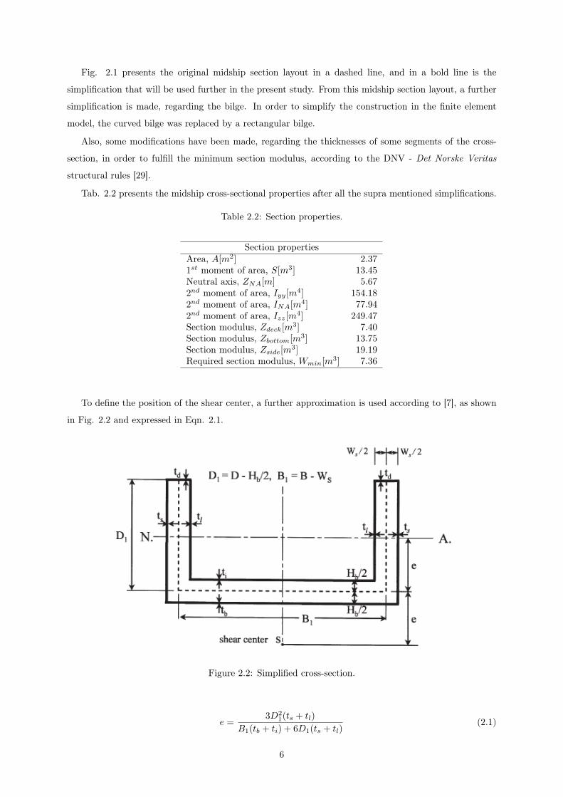
Fig. 2.1 presents the original midship section layout in a dashed line, and in a bold line is the

simplification that will be used further in the present study. From this midship section layout, a further

simplification is made, regarding the bilge. In order to simplify the construction in the finite element

model, the curved bilge was replaced by a rectangular bilge.

Also, some modifications have been made, regarding the thicknesses of some segments of the cross-

section, in order to fulfill the minimum section modulus, according to the DNV - Det Norske Veritas

structural rules [29].

Tab. 2.2 presents the midship cross-sectional properties after all the supra mentioned simplifications.

Table 2.2: Section properties.

Section propertiesArea, A[m2] 2.371st moment of area, S[m3] 13.45Neutral axis, ZNA[m] 5.672nd moment of area, Iyy[m4] 154.182nd moment of area, INA[m4] 77.942nd moment of area, Izz[m4] 249.47Section modulus, Zdeck[m3] 7.40Section modulus, Zbottom[m3] 13.75Section modulus, Zside[m3] 19.19Required section modulus, Wmin[m

3] 7.36

To define the position of the shear center, a further approximation is used according to [7], as shown

in Fig. 2.2 and expressed in Eqn. 2.1.

Figure 2.2: Simplified cross-section.

e =3D2

1(ts + tl)

B1(tb + ti) + 6D1(ts + tl)(2.1)

6

The equivalent thicknesses are defined applying a procedure that consists in redistributing the net

sectional areas of the internal girders by their attached plate, and further dividing the new areas by the

length of the correspondent segment, obtaining in this way a uniform thickness for each segment. Once

this is done, the estimated thicknesses, as well as the shear center position, are given in Tab. 2.3.

Table 2.3: Equivalent thicknesses and shear center location.

D1[m] 15.40B1[m] 23.80ts[mm] 22.16tl[mm] 16.14tb[mm] 19.46ti[mm] 23.00e[m] 9.07

In respect to the original coordinate system, the shear center is located at the center line of the section

at the coordinate z = −8.27m.

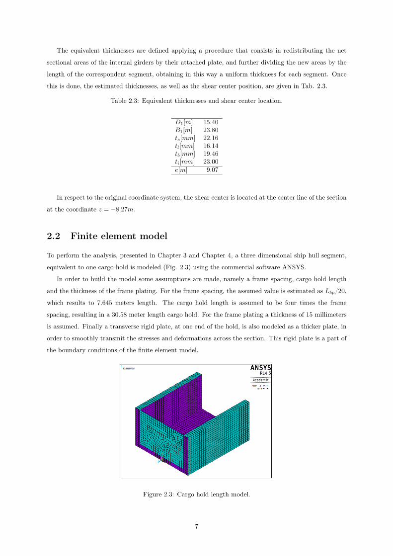
2.2 Finite element model

To perform the analysis, presented in Chapter 3 and Chapter 4, a three dimensional ship hull segment,

equivalent to one cargo hold is modeled (Fig. 2.3) using the commercial software ANSYS.

In order to build the model some assumptions are made, namely a frame spacing, cargo hold length

and the thickness of the frame plating. For the frame spacing, the assumed value is estimated as Lbp/20,

which results to 7.645 meters length. The cargo hold length is assumed to be four times the frame

spacing, resulting in a 30.58 meter length cargo hold. For the frame plating a thickness of 15 millimeters

is assumed. Finally a transverse rigid plate, at one end of the hold, is also modeled as a thicker plate, in

order to smoothly transmit the stresses and deformations across the section. This rigid plate is a part of

the boundary conditions of the finite element model.

Figure 2.3: Cargo hold length model.

7

Element type

The type of elements used is the 8-node quadrilateral shell element (Fig. 2.4). It allows six degrees of

freedom at each node (translations in the nodal x, y and z directions and rotations about the nodal x,

y and z-axes). This type of element has plasticity, stress stiffening, large deflection, and large strain

capabilities. This set of characteristics makes this type of element the most suited for this application.

In ANSYS this type of element is designated as SHELL93.

Figure 2.4: Quadrilateral 8-node shell element.

Boundary conditions

To simulate the interaction between the finite element model of the hull segment with the rest of the ship

hull, the nodes along the lines of one of the ends are constrained in every degree of freedom, while all

other nodes are kept free, such as in a cantilever beam.

Figure 2.5: Boundary conditions applied to the cargo hold length model.

Applied loads

To model the overall loads to which the finite element model is subjected, it is necessary to transform

the loads in equivalent distributed loads or equivalent set of nodal loads and apply them to the specific

nodes of the meshed finite element model of the ship hull.

8

Knowing the bending moment and the second moment of area about the neutral axis of the cross-

section, it is possible to determine the normal stresses σ at any given point:

σi =M

IN.A.di (2.2)

where M is the bending moment, IN.A. is the second moment of area about the neutral axis and di is the

distance of any given point to the neutral axis.

Once the stresses are known, the sectional forces Fi to apply at each node are determined through

the nodal areas, Ai, as:

σi =FiAi

(2.3)

These nodal forces generate an equivalent bending moment, simulating the vertical or horizontal

bending moments as shown in Fig. 2.6.

(a) (b)

Figure 2.6: Equivalent vertical (a) and horizontal (b) bending moments.

For the shear load case, when the overall shear load Q is known, the shear stresses τ are calculated

as:

τ =Q · S∗

t · IN.A.(2.4)

where S∗ is the static shear moment of area and t is the local thickness.

The local shear stresses, based in the nodal areas, can be used to determine the forces to be applied

on each node:

τi =FiAi

(2.5)

9

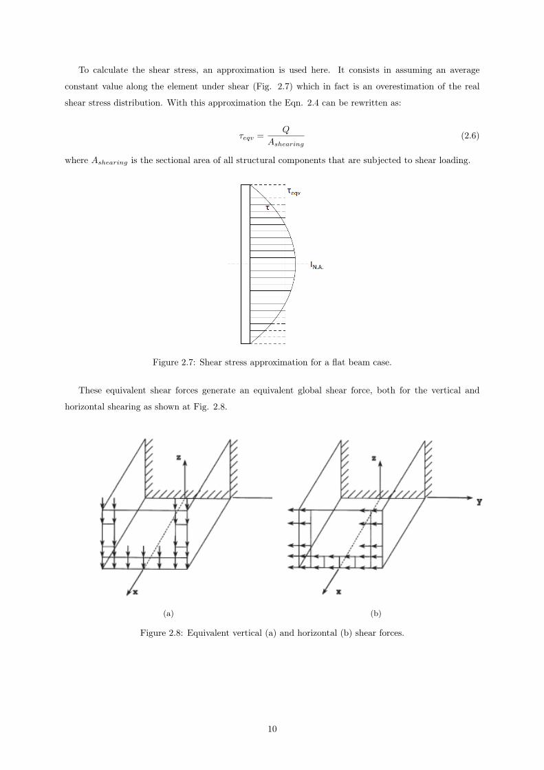
To calculate the shear stress, an approximation is used here. It consists in assuming an average

constant value along the element under shear (Fig. 2.7) which in fact is an overestimation of the real

shear stress distribution. With this approximation the Eqn. 2.4 can be rewritten as:

τeqv =Q

Ashearing(2.6)

where Ashearing is the sectional area of all structural components that are subjected to shear loading.

Figure 2.7: Shear stress approximation for a flat beam case.

These equivalent shear forces generate an equivalent global shear force, both for the vertical and

horizontal shearing as shown at Fig. 2.8.

(a) (b)

Figure 2.8: Equivalent vertical (a) and horizontal (b) shear forces.

10

Nodal areas

An important concept at this point of the study is the one of the nodal area. This area is the area linked

to a specific finite element node (Fig. 2.9). These areas are obtained by multiplying half the distance

between two consecutive nodes, h, and the thickness of the respective plates. This procedure is repeated

for each node as much times as the number of segments that share the considered node.

A =∑i

hiti (2.7)

The structure analyzed here, only has three different types of nodal area configurations with two,

three or four branches as can be seen on Fig. 2.9.

(a) (b) (c)

Figure 2.9: Different nodal area configurations: a) node shared by one or two elements; b) node sharedby three elements; c) node shared by four elements.

11

Chapter 3

Ship hull structure subjected to

bending load

The bending moment acting upon a ship hull can be divided in a vertical and horizontal component. The

sea state along with the longitudinal weight and buoyancy distributions are the principal factors governing

these components of the bending moments. Classification society rules provide the design values for these

loads. In the present analysis the design values, according to DNV - Det Norske Veritas, are used.

3.1 Vertical bending moment

The design vertical bending moment, according to classification society rules, is divided in two compo-

nents: the stillwater and the wave induced bending moments:

MT =MS +MW (3.1)

The stillwater bending moments along the ship length, for sagging and hogging conditions, are given

by:

MS = ksmMSO (3.2)

MSO = −0.065CWL2B(CB + 0.7) (kN.m) in sagging (3.3)

= CWL2B(0.1225− 0.015CB) (kN.m) in hogging (3.4)

where L is the length between perpendiculars of the ship, ksm is a distribution factor, as shown at Fig.

3.1, and CW is the wave coefficient given as:

CW = 10.75−(300− L100

)1.5

(3.5)

12

The wave induced bending moments along the length of the ship are given by:

MW = kwmMWO (3.6)

MWO = −0.11αCWL2B(CB + 0.7) (kN.m) in sagging (3.7)

= 0.19αCWL2BCB (kN.m) in hogging (3.8)

where α = 1 is for seagoing conditions and α = 0.5 for sheltered water conditions, and kwm is a distribution

factor as shown at Fig. 3.1. For this analysis α has its unitary value.

0 0.2 0.4 0.6 0.8 10

0.2

0.4

0.6

0.8

1

1.2

x/L

ksm

0 0.2 0.4 0.6 0.8 10

0.2

0.4

0.6

0.8

1

1.2

x/L

kwm

Figure 3.1: Stillwater design bending moment distribution (left), wave induced design bending momentdistribution (right).

The estimated values for both stillwater and wave-induced design bending moments are presented in

Tab. 3.1.

Table 3.1: Vertical bending moments.

Stillwater bending momentsMSsagging

[kN.m] -478222MShogging

[kN.m] 614467Wave-induced bending momentsMWsagging [kN.m] -809298MWhogging

[kN.m] 673053

Summing the bending moment components, both for sagging and hogging cases, according to Eqn.

3.1, it can be observed that the total design bending moment, in absolute value, is approximately the

same for both conditions. Due to that fact, the hogging bending load case is chosen, MThog= 1287520

kN.m, to be used in the analysis.

13

3.2 Horizontal bending moment

According to the classification society rules, the desing wave-induced bending moment for the horizontal

bending load is given by:

MWH = 0.22L9/4(T + 0.3B)CB

[1− cos

(360

x

L

)](kN.m) (3.9)

where T represents the considered draft.

By plotting the trigonometric parcel of Eqn. 3.9, it is possible to obtain the horizontal design bending

moment distribution.

0 0.1 0.2 0.3 0.4 0.5 0.6 0.7 0.8 0.9 10

1

2

3

x/L

1−cos( 3

60x L

)

Figure 3.2: Horizontal design bending moment distribution.

Considering the distribution shape represented in Fig. 3.2, is clear that the maximum bending moment

occurs when x/L = 0.5, which in fact is the midship. Computing its value, according to Eqn. 3.9, the

estimated value is MWH = 437316 kN.m.

14

3.3 Finite element analysis

Prior to the presentation and discussion of the results according to the procedures described on Chapter

2, it is important to mention that the results obtained by the finite element method are affected by the

particularities of the finite element model. It is expected that stress concentrations may appear, namely

in the proximity of the fully-constrained end of the FE model. Since the boundary conditions applied to

the FE model approximately represent the real case, these stress concentrations are not to be taken into

consideration, for in the real case they would not exist. Hence the readings of the results will be taken

at mid-length of the FE model, at a position where they are as far as possible away from the constrained

end and from the free-end where the nodal forces are applied.

Another important factor, visible throughout the axial stress analysis, is the shear lag effect. This

happens when there are interconnected concurrent plates so that relative displacements between them

cannot occur. This effect leads to a non-uniform axial stress distribution due to a considerable increase

on the stress values on the region when these intersections occur.

Concerning the shear stress results, it is known that its values are considerably affected by the thickness

variations, and hence, notorious discontinuities are expected at the regions where the structure elements

intersect each other.

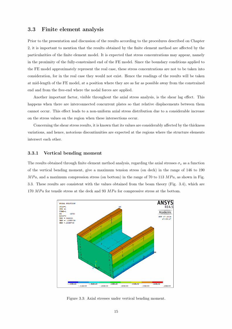
3.3.1 Vertical bending moment

The results obtained through finite element method analysis, regarding the axial stresses σx as a function

of the vertical bending moment, give a maximum tension stress (on deck) in the range of 146 to 190

MPa, and a maximum compression stress (on bottom) in the range of 70 to 113 MPa, as shown in Fig.

3.3. These results are consistent with the values obtained from the beam theory (Fig. 3.4), which are

170 MPa for tensile stress at the deck and 93 MPa for compressive stress at the bottom.

Figure 3.3: Axial stresses under vertical bending moment.

15

The normal stresses taken along the depth of the hull at the side shell at mid-length of the FE model,

are presented in Fig. 3.4, demonstrate tensile stresses on deck of 159 MPa and compressive stresses

on the bottom of 86 MPa, which leads to a difference of about 6% for tensile and 8% for compressive

stresses with respect to the results estimated by the beam theory,

0 5 10 15−100

0

100

200

z[m]

σx[M

Pa]

Beam theoryFEM

Figure 3.4: Axial normal stress distribution along the side shell, under vertical bending moment, obtainedby beam theory (solid line) and FEM (dashed line).

−10 0 10−100

−80

−60

−40

y[m]

σx[M

Pa]

L = 0.0 mL = 15.3 mL = 20.0 m

Figure 3.5: Evolution of the axial stress distribution on the bottom, across the length of the model,measured on the free end (solid line), at half length of the model (dashed line) and at about two thirdsof the model length (dashdotted line).

Analyzing Figs. 3.3 and 3.5, it is possible to observe the effects of the stress concentrations near the

fixed end of the FE model, and a very irregular stress distribution at the free end of the model, where

the loads are applied.

Other important factor to check is the von Mises yield stress criterion. According to this criterion,

a material is said to start yielding when its von Mises stress σv reaches the material yield strength σy.

The von Mises stresses are computed accordingly to:

σv =

√(σ1 − σ2)2 + (σ2 − σ3)2 + (σ1 − σ3)2

2(3.10)

where σ1, σ2 and σ3 are the principal stresses measured at the considered point.

16

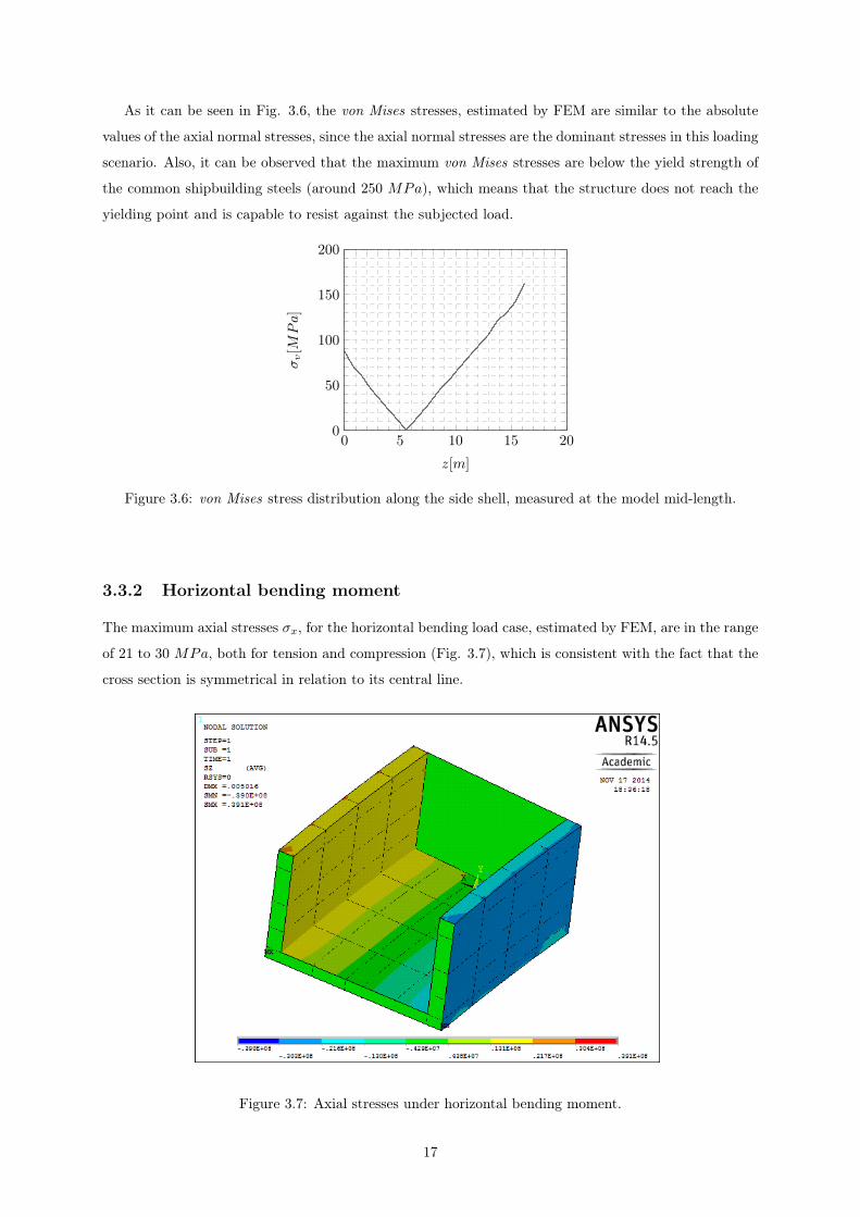
As it can be seen in Fig. 3.6, the von Mises stresses, estimated by FEM are similar to the absolute

values of the axial normal stresses, since the axial normal stresses are the dominant stresses in this loading

scenario. Also, it can be observed that the maximum von Mises stresses are below the yield strength of

the common shipbuilding steels (around 250 MPa), which means that the structure does not reach the

yielding point and is capable to resist against the subjected load.

0 5 10 15 200

50

100

150

200

z[m]

σv[M

Pa]

Figure 3.6: von Mises stress distribution along the side shell, measured at the model mid-length.

3.3.2 Horizontal bending moment

The maximum axial stresses σx, for the horizontal bending load case, estimated by FEM, are in the range

of 21 to 30 MPa, both for tension and compression (Fig. 3.7), which is consistent with the fact that the

cross section is symmetrical in relation to its central line.

Figure 3.7: Axial stresses under horizontal bending moment.

17

−10 0 10

−20

0

20

y[m]σ[M

Pa]

Beam theoryFEM

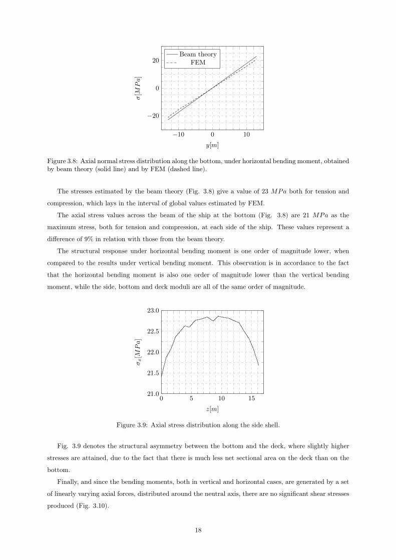
Figure 3.8: Axial normal stress distribution along the bottom, under horizontal bending moment, obtainedby beam theory (solid line) and by FEM (dashed line).

The stresses estimated by the beam theory (Fig. 3.8) give a value of 23 MPa both for tension and

compression, which lays in the interval of global values estimated by FEM.

The axial stress values across the beam of the ship at the bottom (Fig. 3.8) are 21 MPa as the

maximum stress, both for tension and compression, at each side of the ship. These values represent a

difference of 9% in relation with those from the beam theory.

The structural response under horizontal bending moment is one order of magnitude lower, when

compared to the results under vertical bending moment. This observation is in accordance to the fact

that the horizontal bending moment is also one order of magnitude lower than the vertical bending

moment, while the side, bottom and deck moduli are all of the same order of magnitude.

0 5 10 1521.0

21.5

22.0

22.5

23.0

z[m]

σx[M

Pa]

Figure 3.9: Axial stress distribution along the side shell.

Fig. 3.9 denotes the structural asymmetry between the bottom and the deck, where slightly higher

stresses are attained, due to the fact that there is much less net sectional area on the deck than on the

bottom.

Finally, and since the bending moments, both in vertical and horizontal cases, are generated by a set

of linearly varying axial forces, distributed around the neutral axis, there are no significant shear stresses

produced (Fig. 3.10).

18

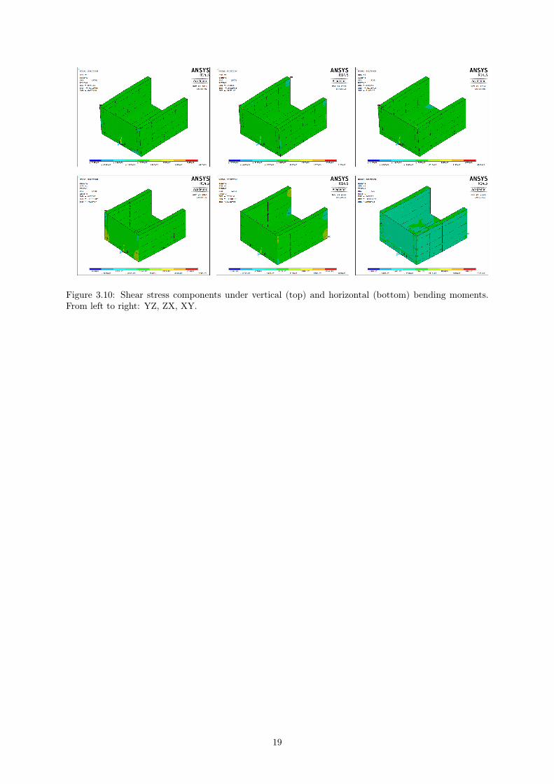
Figure 3.10: Shear stress components under vertical (top) and horizontal (bottom) bending moments.From left to right: YZ, ZX, XY.

19

Chapter 4

Ship hull structure subjected to shear

load

4.1 Vertical shear forces

The vertical shear forces acting on a ship while she’s sailing are divided in stillwater shear forces, caused

by the weight and buoyancy distributions; and in wave induced shear forces, caused by the encountered

sea effects.

The classification society rule values for the stillwater shear forces along the length of the ship, both

in sagging and hogging are determined as:

QS = ksqQSO (4.1)

QSO = 5MSO

L(kN) (4.2)

whereMSO are the stillwater design bending moment as determined in Chapter 3, and ksq is a distribution

factor as illustrated at Fig. 4.1.

The wave-induced shear force rule values can be positive or negative, depending on the sign of the

stillwater shear force.

QWP = 0.3βkwqpCWLB(CB + 0.7) (kN) (4.3)

QWN = −0.3βkwqnCWLB(CB + 0.7) (kN) (4.4)

where β is a factor with unitary a value for seagoing conditions (in use) and 0.5 for sheltered waters and

kwqp and kwqn are the distribution factors varying as shown on Fig. 4.1.

20

0 0.2 0.4 0.6 0.8 10

0.2

0.4

0.6

0.8

1

1.2

x/L

ksq

0 0.2 0.4 0.6 0.8 10

0.2

0.4

0.6

0.8

1

1.2

x/L

kwq

Figure 4.1: Stillwater design shear force distribution (left), wave induced design shear force distributionsboth for positive (solid line, kwqp) and negative (dashed line, kwqn) cases (right).

Testing the different possible scenarios resulting from Eqns. 4.1 to 4.4, and considering the distribu-

tions from Fig. 4.1, the conclusion is that the maximum vertical design shear force case takes place when

x/L ∈ [0.7; 0.85]. The structural analysis is performed at x/L = 0.7, since it coincides with a transverse

bulkhead and the division between the cargo holds. The results are presented at Tab. 4.1.

Table 4.1: Vertical design shear forces.

Stillwater shear forcesQS−[kN ] -15638QS+[kN ] 20094Wave-induced shear forcesQWN [kN ] -12025QWP [kN ] 14435

Summing the stillwater and wave-induced shear loads, results in an higher load for the positive shear

force scenario. The obtained final vertical shear force is QT = 34529 kN.

21

4.2 Wave-induced horizontal shear forces

The horizontal wave-induced design shear force along the ship length is given by the classification society

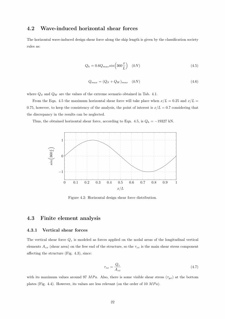
rules as:

Qh = 0.6Qmaxsin(360

x

L

)(kN) (4.5)

Qmax = (QS +QW )max (kN) (4.6)

where QS and QW are the values of the extreme scenario obtained in Tab. 4.1.

From the Eqn. 4.5 the maximum horizontal shear force will take place when x/L = 0.25 and x/L =

0.75, however, to keep the consistency of the analysis, the point of interest is x/L = 0.7 considering that

the discrepancy in the results can be neglected.

Thus, the obtained horizontal shear force, according to Eqn. 4.5, is Qh = −19327 kN.

0 0.1 0.2 0.3 0.4 0.5 0.6 0.7 0.8 0.9 1

−1

0

1

x/L

sin( 36

0x L

)

Figure 4.2: Horizontal design shear force distribution.

4.3 Finite element analysis

4.3.1 Vertical shear forces

The vertical shear force Qz is modeled as forces applied on the nodal areas of the longitudinal vertical

elements Azx (shear area) on the free end of the structure, so the τzx is the main shear stress component

affecting the structure (Fig. 4.3), since:

τzx =QzAzx

(4.7)

with its maximum values around 97 MPa. Also, there is some visible shear stress (τyx) at the bottom

plates (Fig. 4.4). However, its values are less relevant (on the order of 10 MPa).

22

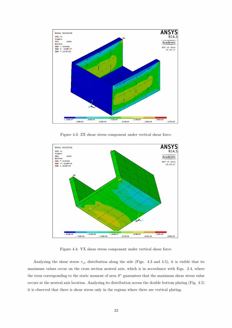
Figure 4.3: ZX shear stress component under vertical shear force.

Figure 4.4: YX shear stress component under vertical shear force.

Analyzing the shear stress τzx distribution along the side (Figs. 4.3 and 4.5), it is visible that its

maximum values occur on the cross section neutral axis, which is in accordance with Eqn. 2.4, where

the term corresponding to the static moment of area S∗ guarantees that the maximum shear stress value

occurs at the neutral axis location. Analyzing its distribution across the double bottom plating (Fig. 4.5)

it is observed that there is shear stress only in the regions where there are vertical plating.

23

0 5 10 150

20

40

60

80

z[m]

τ zx[M

Pa]

0 5 10 15 20 250

10

20

30

40

y[m]

τ zx[M

Pa]

Figure 4.5: ZX shear stress component measured at the model mid-length along the side (left) and alongthe double bottom (right).

4.3.2 Horizontal shear forces

In this load case, the shear force Qy is modeled as forces applied on the nodal areas of longitudinal

horizontal elements. Thus, the main shear stress component affecting the structure is τyx, as shown in

Fig. 4.6, with its values around 74 MPa.

Figure 4.6: YX shear stress component under horizontal shear force.

Besides the dominant τyx shear stress component, as in the vertical shear force load case, there is a

residual shear stress propagation trough the plating in the normal orientation to the load, in the present

case, the τzx component. Once again, its values are considerably lower, around 30 MPa (Fig. 4.7).

24

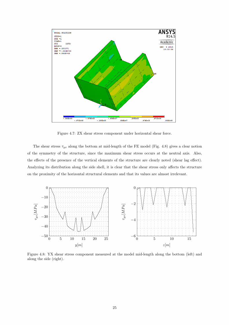
Figure 4.7: ZX shear stress component under horizontal shear force.

The shear stress τyx along the bottom at mid-length of the FE model (Fig. 4.8) gives a clear notion

of the symmetry of the structure, since the maximum shear stress occurs at the neutral axis. Also,

the effects of the presence of the vertical elements of the structure are clearly noted (shear lag effect).

Analyzing its distribution along the side shell, it is clear that the shear stress only affects the structure

on the proximity of the horizontal structural elements and that its values are almost irrelevant.

0 5 10 15 20 25−50

−40

−30

−20

−10

0

y[m]

τ yx[M

Pa]

0 5 10 15−6

−4

−2

0

z[m]

τ yx[M

Pa]

Figure 4.8: YX shear stress component measured at the model mid-length along the bottom (left) andalong the side (right).

25

Chapter 5

Ship hull structure subjected to

torsional loading

The distribution of the torsional moment along the ship length depends on the cargo load distribution,

both longitudinally and transversely, as well as on the ship advance direction relatively to the encountered

waves, which can produce asymmetric loads on the hull. The torsional moment T is divided in two

components, namely the St. Venant torsional moment TS and warping torsional moment Tω [28], hence:

T = TS + Tω (5.1)

The St. Venant component accounts for the torsion effects assuming that there are no in-plane

deformations, i.e. a plane cross section remains plane during the twist. This kind of torsion is only verified

in circular closed cross sections, while in the remaining cases the warping component must be considered,

since the cross sections no longer remain in plane during the twist. These warping deformations vary

with the rate of twist and as a function of the position across the cross section.

5.1 Bi-moment method analysis

In the preliminary design stages, when the torsional loading is not yet know, the application of a simplified

procedure for structural analysis is very important. This approximate method gives a general procedure

for calculating the shear and flexural warping stresses as well as the torsional deformations induced in

open ships by torsional loading. Is based on the sectorial properties of the ship section, which are obtained

using a simplified idealization of the ship section configuration [28].

The shear and flexural (normal) warping stresses are calculated as follows:

τ(ω) =T (ω) · S(ω)J(ω)t

(5.2)

σ(ω) =ω ·M(ω)

J(ω)(5.3)

26

where T (ω) is the warping torsional moment, S(ω) is the sectorial static moment,M(ω) is the bi-moment,

J(ω) is the sectorial moment of inertia (or warping constant of the section), ω is the sectorial coordinate

and t is the thickness.

T (ω) = −EJ(ω)d3φ

dx3(5.4)

M(ω) = −EJ(ω)d2φ

dx2(5.5)

In order to proceed with the determination of the warping stresses, the sectorial properties of the ship

section (i.e. ω, S(ω) and J(ω)) and the solution of the torsion equation (i.e. φ(x)) must be determined.

The differential equation for non-uniform torsion, equivalent to Eqn. 5.1, is given by:

GJtdφ

dx− EJ(ω)d

3φ

dx3= T (5.6)

where E is the Young modulus, G is the shear modulus, Jt is the torsional modulus and T is the sectional

torque applied to the structure.

Equation 5.6 can be rewritten as:

dφ

dx− k2 d

3φ

dx3=

T

GJt(5.7)

where:

k2 =EJ(ω)

GJt(5.8)

The solution of the differential equation (Eqn. 5.7) depends on the boundary conditions and on the

torque characteristics expressed below as:

A) Fixed end with free warping

This boundary condition, satisfy:

φ =d2φ

dx2= 0 (5.9)

B) Fixed end with constrained warping

This boundary condition, satisfy:

φ =dφ

dx= 0 (5.10)

Applied torque

The magnitude and distribution of the torsional loading, acting upon a ship hull, depend on a multitude

of factors, namely the hull form, the sea state, the cargo distribution, the shear center position and etc.

27

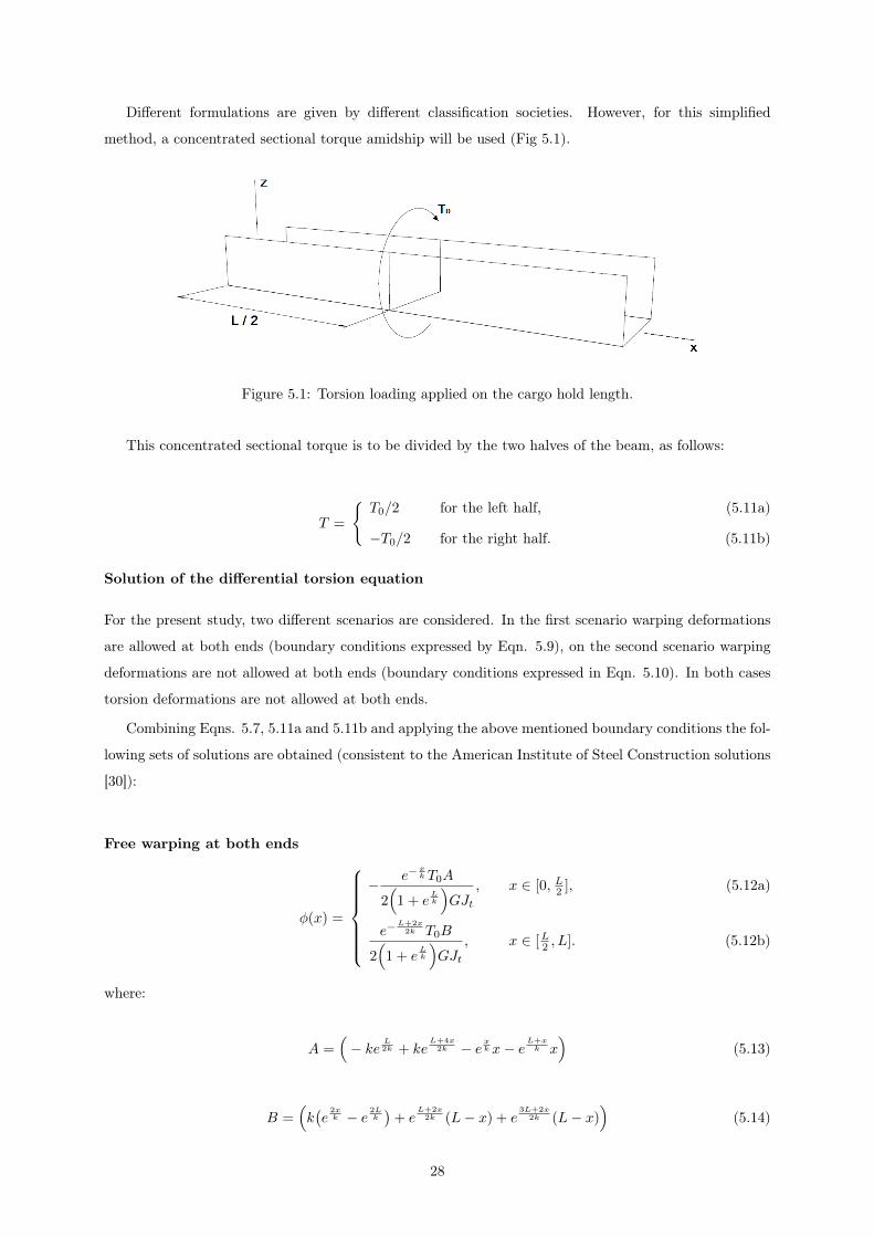
Different formulations are given by different classification societies. However, for this simplified

method, a concentrated sectional torque amidship will be used (Fig 5.1).

Figure 5.1: Torsion loading applied on the cargo hold length.

This concentrated sectional torque is to be divided by the two halves of the beam, as follows:

T =

{T0/2 for the left half, (5.11a)

−T0/2 for the right half. (5.11b)

Solution of the differential torsion equation

For the present study, two different scenarios are considered. In the first scenario warping deformations

are allowed at both ends (boundary conditions expressed by Eqn. 5.9), on the second scenario warping

deformations are not allowed at both ends (boundary conditions expressed in Eqn. 5.10). In both cases

torsion deformations are not allowed at both ends.

Combining Eqns. 5.7, 5.11a and 5.11b and applying the above mentioned boundary conditions the fol-

lowing sets of solutions are obtained (consistent to the American Institute of Steel Construction solutions

[30]):

Free warping at both ends

φ(x) =

− e−

xk T0A

2(1 + e

Lk

)GJt

, x ∈ [0, L2 ], (5.12a)

e−L+2x

2k T0B

2(1 + e

Lk

)GJt

, x ∈ [L2 , L]. (5.12b)

where:

A =(− ke L

2k + keL+4x

2k − e xk x− e

L+xk x

)(5.13)

B =(k(e

2xk − e 2L

k

)+ e

L+2x2k (L− x) + e

3L+2x2k (L− x)

)(5.14)

28

Constrained warping at both ends

φ(x) =

− e−

xk T0C

2(1 + e

L2k

)GJt

, x ∈ [0, L2 ], (5.15a)

e−L+2x

2k T0D

2(1 + e

L2k

)GJt

, x ∈ [L2 , L]. (5.15b)

where:

C =(− ke L

2k − e xk (k + x) + ke

2xk + e

L+2x2k (k − x)

)(5.16)

D =(k(e

2xk − e 3L

2k

)+ e

L+2x2k (k + L− x) + e

L+xk (−k + L− x)

)(5.17)

5.1.1 Simplified structural response

In order to simplify the computations, the cross sectional configuration of the double-skin structure of

an open ship is simplified as a thin-walled open section [28]. This procedure, consists in transforming a

section, like the one shown on Fig. 5.2a, on a simplified one, Fig. 5.2b, considering its effective bottom

and side structures thicknesses. The sectional areas of the horizontal and vertical girders, on the side

shell and double bottom respectively, are idealized as lumped areas.

(a) (b)

Figure 5.2: (a) Typical container ship section. (b) Idealization of the ship section.

For the present case study, the original section given in Fig. 2.1, is simplified into the idealization

presented at Fig. 5.3.

The general relation between the main geometrical properties (e.g. beam and draft) of the original

structure is expressed by the following equation:

Didealization =Dexternal +Dinternal

2(5.18)

where D is a generic main dimension.

29

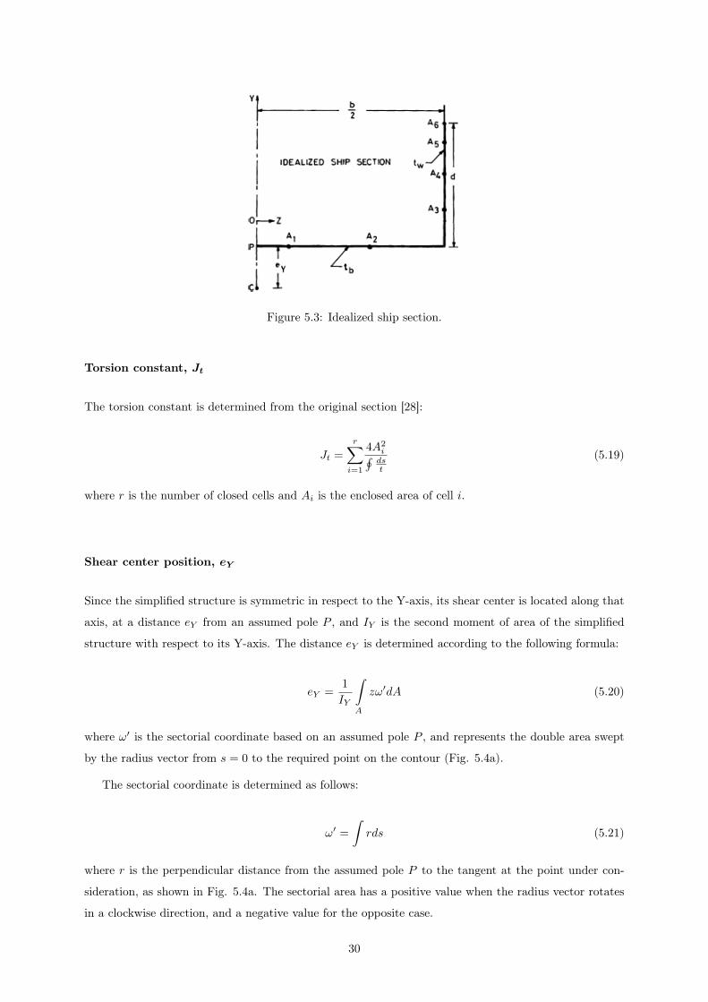
Figure 5.3: Idealized ship section.

Torsion constant, Jt

The torsion constant is determined from the original section [28]:

Jt =

r∑i=1

4A2i∮dst

(5.19)

where r is the number of closed cells and Ai is the enclosed area of cell i.

Shear center position, eY

Since the simplified structure is symmetric in respect to the Y-axis, its shear center is located along that

axis, at a distance eY from an assumed pole P , and IY is the second moment of area of the simplified

structure with respect to its Y-axis. The distance eY is determined according to the following formula:

eY =1

IY

∫A

zω′dA (5.20)

where ω′ is the sectorial coordinate based on an assumed pole P , and represents the double area swept

by the radius vector from s = 0 to the required point on the contour (Fig. 5.4a).

The sectorial coordinate is determined as follows:

ω′ =

∫rds (5.21)

where r is the perpendicular distance from the assumed pole P to the tangent at the point under con-

sideration, as shown in Fig. 5.4a. The sectorial area has a positive value when the radius vector rotates

in a clockwise direction, and a negative value for the opposite case.

30

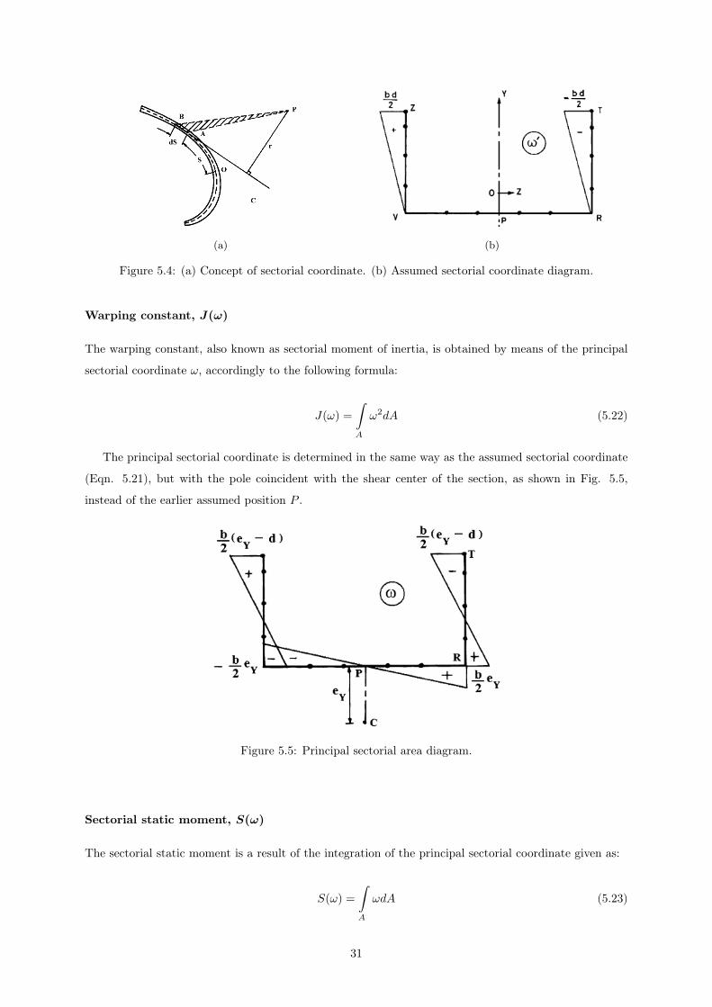
(a) (b)

Figure 5.4: (a) Concept of sectorial coordinate. (b) Assumed sectorial coordinate diagram.

Warping constant, J(ω)

The warping constant, also known as sectorial moment of inertia, is obtained by means of the principal

sectorial coordinate ω, accordingly to the following formula:

J(ω) =

∫A

ω2dA (5.22)

The principal sectorial coordinate is determined in the same way as the assumed sectorial coordinate

(Eqn. 5.21), but with the pole coincident with the shear center of the section, as shown in Fig. 5.5,

instead of the earlier assumed position P .

Figure 5.5: Principal sectorial area diagram.

Sectorial static moment, S(ω)

The sectorial static moment is a result of the integration of the principal sectorial coordinate given as:

S(ω) =

∫A

ωdA (5.23)

31

5.1.2 Results and analysis

For the procedures described in the previous section, two main classes of inputs are required. The material

and geometric properties of the simplified structure (Tab. 5.1) and the applied torsional load.

Table 5.1: Structural input parameters.

Steel propertiesYoung modulus, E[GPa] 200.0Shear modulus, G[GPa] 79.3

Section propertiesBeam, b[m] 23.80Depth, d[m] 15.40Sheer strake height, a[m] 2.40Bottom thickness, tb[mm] 37.00Side thickness, tw1[mm] 30.00Sheer strake thickness, tw2[mm] 42.34

Lumped areas, AiA1,2, [m2] 2.16E-2A3,4, [m2] 2.20E-2A5, [m2] 2.64E-2A6, [m2] 8.28E-2

As discussed in section 5.1, the torsionl load applied to the structure is a concentrated sectional

moment amidship. This load is determined according to classification society rules wave-induced torsional

moment equation (Eqn. 5.24) computed at midship. The estimated value is 144 MN.m.

MWT = KT1L5/4(T + 0.3B)CBze ±KT2L

4/3B2CSWP (kN.m) (5.24)

where

KT1 = 1.4sin(360

x

L

)(5.25)

KT2 = 0.13(1− cos(360

x

L

)) (5.26)

CSWP =AWP

LB(5.27)

and ze is the height of the neutral axis. Since the waterplane area AWP is not known, the waterplane

coefficient CSWP (Eqn. 5.27) has to be assumed. The same logic of “worst case scenario” is applied, so

the assumption is that the waterplane coefficient has an unitary value (CSWP = 1).

32

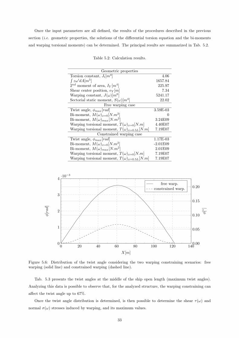
Once the input parameters are all defined, the results of the procedures described in the previous

section (i.e. geometric properties, the solutions of the differential torsion equation and the bi-moments

and warping torsional moments) can be determined. The principal results are summarized in Tab. 5.2.

Table 5.2: Calculation results.

Geometric propertiesTorsion constant, Jt[m4] 4.06∫zω′dA[m5] 1657.84

2nd moment of area, IY [m4] 225.97Shear center position, eY [m] 7.34Warping constant, J(ω)[m6] 5241.17Sectorial static moment, S(ω)[m4] 22.02

Free warping caseTwist angle, φmax[rad] 3.59E-03Bi-moment, M(ω)x=0[N.m

2] 0Bi-moment, M(ω)max[N.m

2] 3.24E09Warping torsional moment, T (ω)x=0[N.m] 4.40E07Warping torsional moment, T (ω)x=0.5L[N.m] 7.19E07

Constrained warping caseTwist angle, φmax[rad] 1.17E-03Bi-moment, M(ω)x=0[N.m

2] -2.01E09Bi-moment, M(ω)max[N.m

2] 2.01E09Warping torsional moment, T (ω)x=0[N.m] 7.19E07Warping torsional moment, T (ω)x=0.5L[N.m] 7.19E07

0 20 40 60 80 100 120 1400

1

2

3

4

0.00

0.05

0.10

0.15

0.20

·10−3

X[m]

φ[rad]

φ[◦]

free warp.constrained warp.

Figure 5.6: Distribution of the twist angle considering the two warping constraining scenarios: freewarping (solid line) and constrained warping (dashed line).

Tab. 5.3 presents the twist angles at the middle of the ship open length (maximum twist angles).

Analyzing this data is possible to observe that, for the analyzed structure, the warping constraining can

affect the twist angle up to 67%.

Once the twist angle distribution is determined, is then possible to determine the shear τ(ω) and

normal σ(ω) stresses induced by warping, and its maximum values.

33

Table 5.3: Twist angle at the middle of the ship open length.

Warping φ[rad] φ[◦]Free 3.59E-03 0.206Constrained 1.17E-03 0.067

Fig. 5.7 represents the distributions of the shear and normal stresses induced by warping on a simple

beam. In the shear stress case, the maximum value τω1 is attained in the flange at a position symmetrical

to the shear center position in relation with the base line, being zero at the flange top. However in the

present case study the shear stress distribution (Fig. 5.8) must take into consideration the thickness

variation in the side structure and also the contribution of the girders for the sectorial static moment, as

stated in Eqn. 5.2. These factors produce a significant change, since the shear stress at the top of the

side structure is not zero anymore.

(a) (b)

Figure 5.7: Channel section cross-sectional distribution of shear (a) and normal (b) stresses due towarping.

Regarding the normal stress distribution, there is no difference between the example shown in Fig.

5.7 and the studied structure, with its maximum value being on the flange tip and attaining zero value

at a position symmetrical to the shear center position in relation to the base line (z = 7.4m).

At this point it is possible to determine the warping induced stresses at any point of the simplified

structure. It is observed that the higher values of the shear stress are found (Tab. 5.4 and Fig. 5.9) at the

mid-length of the beam model, and are equal for both warping-free and constrained warping cases. Also

in the constrained warping case the shear stresses have the same values at the mid-length and extremities.

34

0 2 4 6 8 10 12 14 160

0.2

0.4

0.6

0.8

1

1.2

Z[m]

τ(ω

)/ τ

(ω) m

ax

Figure 5.8: Distribution of the dimensionless warping induced shear stress from the top of the sidestructure to its connection with the bottom structure.

For the normal stress case, its maximum values are observed at the beam models mid-length (Fig.

5.10) and with a value about 38% higher for the warping free model.

Table 5.4: Maximum stress values (values in Pa).

free warping const. warping diff. [%]τ(ω)max 9.80E06 9.80E06 0τ(ω)sheer strake 2.57E06 2.57E06 0τ(ω)bilge 4.05E06 4.05E06 0τ(ω)keel -3.50E06 -3.50E06 0σ(ω)sheer strake 5.93E07 3.68E07 38σ(ω)bilge -5.40E07 -3.35E07 38

0 20 40 60 80 100 120 140−1

−0.5

0

0.5

1·107

X[m]

τ(ω

)[Pa]

free warp.constrained warp.

Figure 5.9: Warping induced maximum shear stress distribution along the length considering the twowarping constraining scenarios: free warping (solid line) and constrained warping (dashed line).

35

0 20 40 60 80 100 120 140−4

−2

0

2

4

6·107

X[m]

σ(ω

)[Pa]

free warp.constrained warp.

Figure 5.10: Warping induced normal stress distribution at sheer strake along the length considering thetwo warping constraining scenarios: free warping (solid line) and constrained warping (dashed line).

Another stress component that was not yet considered (because its effects are neglectable) is the

pure torsional shear stress. This component is always present on a cross-section of a member subject to

torsion, and its maximum values are determined according to:

τt = Gtdφ

dx(5.28)

In a contrary to the warping induced shear stress, the pure torsional shear stress is not constant

trough the thickness of the element, varying linearly between the two edges of the element (Fig. 5.11).

Consequently, the maximum value of this shear stress component is found at the thickest element of the

cross-section, in the present case the sheer strake.

Figure 5.11: Channel cross-sectional pure torsional shear stress distribution.

36

In order to determine the total shear stress fv at any determined point of the cross-section, the

different shear stress components are combined using the superposition principle according to:

fv = τ(ω)± τt (5.29)

Since the maximum values for the pure torsional shear stress are of the order of 0.3 MPa (Fig. 5.12)

and the ones from the warping induced shear stress are of the order of 10 MPa (Fig. 5.9), the former

component might be considered neglectable when compared to the latter.

At a scenario where the pure torsional shear stress is higher, its contribution represents only about

4.7% of the total shear stress (Fig. 5.13).

0 20 40 60 80 100 120 140−4

−2

0

2

4·105

[m]

τ t[Pa]

free warp.constrained warp.

Figure 5.12: Pure torsional shear stress distribution at sheer strake along the length considering the twowarping constraining scenarios: free warping (solid line) and constrained warping (dashed line).

0 2 4 6 8 10 12 14 160

2

4

6

·106

[m]

τ[Pa]

τ(ω)τtfv

Figure 5.13: Distribution of the total shear stress and its components along the side structure at across-section at x=0 in an unrestricted warping scenario.

37

5.2 Finite element analysis

Another approach applied here is the finite element analysis of the open ship structure subjected to

torsional loading. This option represents a much more exhaustive and time consuming task, since it

requires a somewhat complex FE structural model. For this reason, this approach can only be used at a

later stage of the design process when more details are known.

At this point of the study another aspect is to be considered. The differences of the structural

responses in the cases where the ship structure is open, partially closed or fully closed, are investigated

through the analysis of three different three dimensional FE models.

5.2.1 Model generation

For this analysis, the whole simplified ship hull structure is modeled. The model consists on the replication

of the model used in the previous sections, in such way that it now forms a cylindrical body with 122.32

meters length, divided in four cargo holds separated by transversal bulkheads. Also simplified symmetric

bow and stern closings with closed cross-sections are modeled, creating a 154.81 meters length overall

barge-like model.

Three different models are created with the objective of comparing the different structural responses.

The first model (open model, Fig. 5.14a) has four open cargo holds, the second model (partially-closed

model, Fig. 5.14b) has its forward and after holds closed and the third model (closed model, Fig. 5.14c)

has all its cargo holds closed, in a “tanker-like” configuration.

The element type and meshing parameters used, are the same as already described in Chapter 2.

38

(a) (b)

(c)

Figure 5.14: (a) Open model. (b) Partially-closed model. (c) Closed model.

Boundary conditions and applied loads

The boundary conditions applied to the FE model are such that all the nodes on both end planes, since

the models have both bow and stern vertical transoms, are constrained in every degree of freedom (Fig.

5.15).

Figure 5.15: Boundary conditions.

39

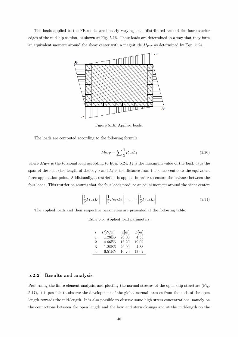
The loads applied to the FE model are linearly varying loads distributed around the four exterior

edges of the midship section, as shown at Fig. 5.16. These loads are determined in a way that they form

an equivalent moment around the shear center with a magnitude MWT as determined by Eqn. 5.24.

Figure 5.16: Applied loads.

The loads are computed according to the following formula:

MWT =∑ 1

2PiaiLi (5.30)

where MWT is the torsional load according to Eqn. 5.24, Pi is the maximum value of the load, ai is the

span of the load (the length of the edge) and Li is the distance from the shear center to the equivalent

force application point. Additionally, a restriction is applied in order to ensure the balance between the

four loads. This restriction assures that the four loads produce an equal moment around the shear center:

∣∣∣∣12P1a1L1

∣∣∣∣ = ∣∣∣∣12P2a2L2

∣∣∣∣ = ... =

∣∣∣∣12P4a4L4

∣∣∣∣ (5.31)

The applied loads and their respective parameters are presented at the following table:

Table 5.5: Applied load parameters.

i P [N/m] a[m] L[m]1 1.28E6 26.00 4.332 4.66E5 16.20 19.023 1.28E6 26.00 4.334 6.51E5 16.20 13.62

5.2.2 Results and analysis

Performing the finite element analysis, and plotting the normal stresses of the open ship structure (Fig.

5.17), it is possible to observe the development of the global normal stresses from the ends of the open

length towards the mid-length. It is also possible to observe some high stress concentrations, namely on

the connections between the open length and the bow and stern closings and at the mid-length on the

40

connection between the inner side and the transversal bulkhead. However these local stress concentrations

will not be regarded.

Figure 5.17: Normal stress under torsional loading.

As can be seen in Fig. 5.17, the normal stresses tend to be higher on the sheer strake region. According

to this, the normal stress distribution along the sheer strake are plotted (Fig. 5.18) for the three different

structural configurations presented before. These plots confirm that the maximum normal stress levels

are much higher for an open structure (45.4MPa) than for a closed structure configuration (9.2MPa).

0 20 40 60 80 100 120 140−4

−2

0

2

4

6·107

X[m]

σx[Pa]

open-deckclosed-deck

partially closed-deck

Figure 5.18: Normal stress distributions at sheer strake along the length for open-deck (solid line), closed-deck (dashed line) and partially closed-deck (dashdotted line) cases.

41

Another important aspect, visible in Fig. 5.18 is the effect of the transversal bulkheads on the normal

stress. These bulkheads are positioned at 30.58m, 61.16m and 91.74m, respectively 1/4, 1/2 and 3/4

of the open length. Its effects are more visible on the open structure configuration and gradually less

visible, until they are almost not noticeable at the closed structure configuration.

Concerning the normal stress distributions along the depth and beam of the hull, they are to be

checked at a section where the stress levels are maximum at the sheer strake. This section is expected

to be the midship section, however as can be seen in Fig. 5.18 the presence of the transversal bulkhead

causes a sudden reduction of the normal stress level at this section, therefore, the chosen section as at

66.5m. Figs. 5.19 and 5.20 show the normal stress distribution along the depth and beam, respectively.

0 2 4 6 8 10 12 14 16 18−6

−4

−2

0

2

4

6·107

Z[m]

σx[Pa]

open-deckclosed-deck

partially closed-deck

Figure 5.19: Normal stress distribution along the depth at a section located at x = 66.5m for open-deck(solid line), closed-deck (dashed line) and partially closed-deck (dashdotted line) cases.

0 2 4 6 8 10 12 14 16 18 20 22 24 26−6

−4

−2

0

2

4

6·107

Y [m]

σx[Pa]

open-deckclosed-deck

partially closed-deck

Figure 5.20: Normal stress distribution along the bottom at a section located at x = 66.5m for open-deck(solid line), closed-deck (dashed line) and partially closed-deck (dashdotted line) cases.

Fig. 5.19 present normal stress distributions that tend to be linear. The plot of the open deck scenario

42

shows that the zero value is attained at the coordinate z = 9.65m. This, represents a deviation of around

16.7% when compared to the extrapolation from the beam model, where this value should occur at a

distance from the base line equal to the shear center distance to the same base line (z = 8.27m). This

observation also means that the normal stress levels are higher at the bottom region than they are on

the deck.

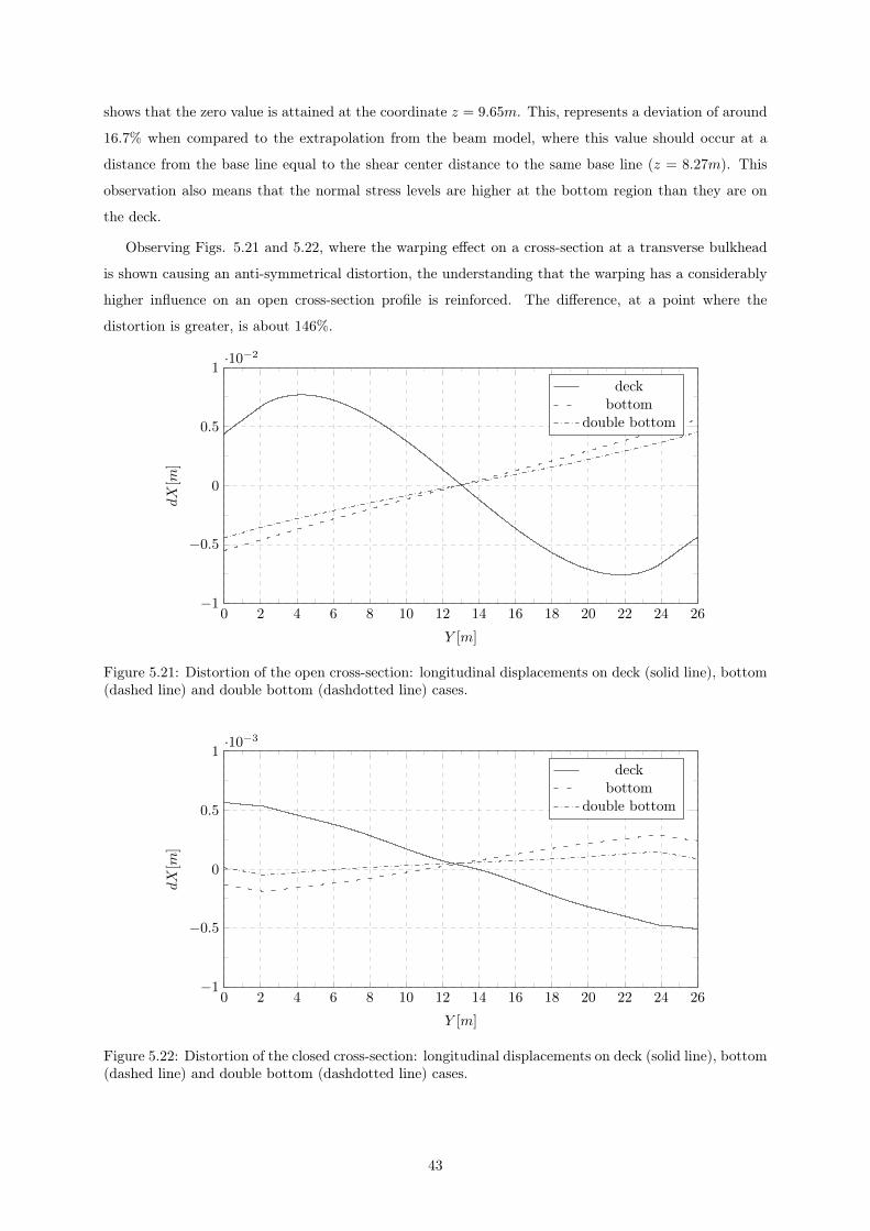
Observing Figs. 5.21 and 5.22, where the warping effect on a cross-section at a transverse bulkhead

is shown causing an anti-symmetrical distortion, the understanding that the warping has a considerably

higher influence on an open cross-section profile is reinforced. The difference, at a point where the

distortion is greater, is about 146%.

0 2 4 6 8 10 12 14 16 18 20 22 24 26−1

−0.5

0

0.5

1·10−2

Y [m]

dX[m

]

deckbottom

double bottom

Figure 5.21: Distortion of the open cross-section: longitudinal displacements on deck (solid line), bottom(dashed line) and double bottom (dashdotted line) cases.

0 2 4 6 8 10 12 14 16 18 20 22 24 26−1

−0.5

0

0.5

1·10−3

Y [m]

dX[m

]

deckbottom

double bottom

Figure 5.22: Distortion of the closed cross-section: longitudinal displacements on deck (solid line), bottom(dashed line) and double bottom (dashdotted line) cases.

43

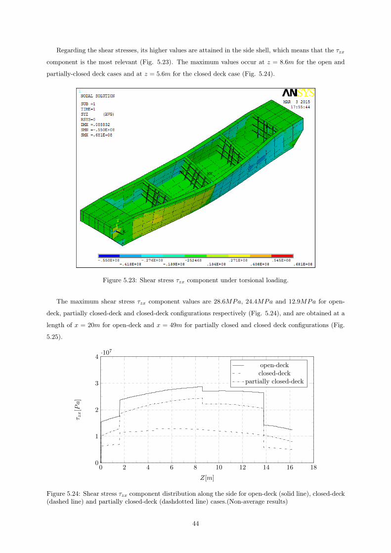
Regarding the shear stresses, its higher values are attained in the side shell, which means that the τzx

component is the most relevant (Fig. 5.23). The maximum values occur at z = 8.6m for the open and

partially-closed deck cases and at z = 5.6m for the closed deck case (Fig. 5.24).

Figure 5.23: Shear stress τzx component under torsional loading.

The maximum shear stress τzx component values are 28.6MPa, 24.4MPa and 12.9MPa for open-

deck, partially closed-deck and closed-deck configurations respectively (Fig. 5.24), and are obtained at a

length of x = 20m for open-deck and x = 49m for partially closed and closed deck configurations (Fig.

5.25).

0 2 4 6 8 10 12 14 16 180

1

2

3

4·107

Z[m]

τ zx[Pa]

open-deckclosed-deck

partially closed-deck

Figure 5.24: Shear stress τzx component distribution along the side for open-deck (solid line), closed-deck(dashed line) and partially closed-deck (dashdotted line) cases.(Non-average results)

44

0 20 40 60 80 100 120 140−4

−2

0

2

4·107

X[m]

τ zx[Pa]

open-deckclosed-deck

partially closed-deck

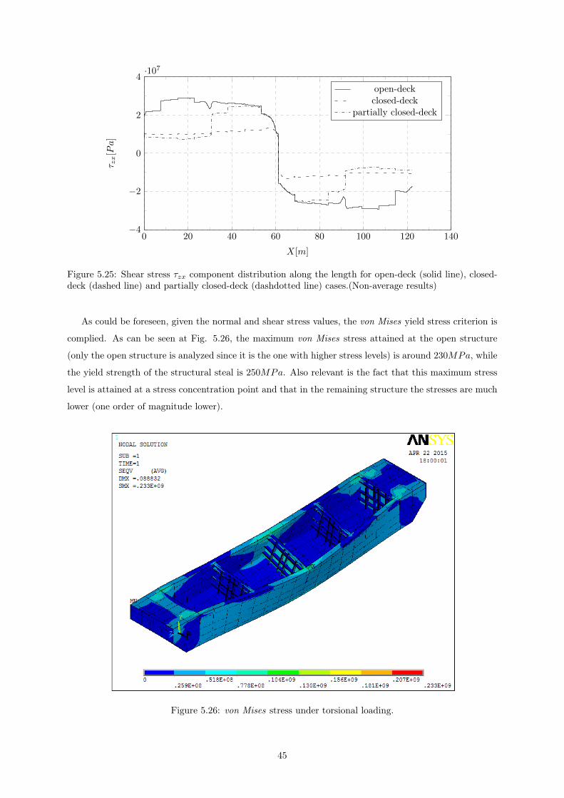
Figure 5.25: Shear stress τzx component distribution along the length for open-deck (solid line), closed-deck (dashed line) and partially closed-deck (dashdotted line) cases.(Non-average results)

As could be foreseen, given the normal and shear stress values, the von Mises yield stress criterion is

complied. As can be seen at Fig. 5.26, the maximum von Mises stress attained at the open structure

(only the open structure is analyzed since it is the one with higher stress levels) is around 230MPa, while

the yield strength of the structural steal is 250MPa. Also relevant is the fact that this maximum stress

level is attained at a stress concentration point and that in the remaining structure the stresses are much

lower (one order of magnitude lower).

Figure 5.26: von Mises stress under torsional loading.

45

5.3 Comparison and discussion

Comparing the axial stress longitudinal distribution given by the two approximate methods (Fig. 5.27)

along the sheer strake, an almost perfect fit of the FEM results between the two limit cases of the bi-

moment method (free and constrained warping) is observed. This fit is only broke due to the warping

stress fluctuation at the presence of the transversal bulkheads and respective deck strips as explained by

Villavicencio et al. 2015 [27].

0 20 40 60 80 100 120 140−4

−2

0

2

4

6·107

X[m]

σx[Pa]

FEMfree warp.

const. warp.

Figure 5.27: Comparison between open-deck finite element method and free and constrained warping bythe bi-moment method for axial stress results along the sheer strake.

As for the situation of the axial stress distribution across the bottom, at a section where the stresses

levels are higher (theoretically the midship section, however due to warping stress fluctuations in the

FEM model this section is slightly forward) it is possible to see (Fig. 5.28) a quite good fit between the

results and particularly good at the extreme values.

46

0 2 4 6 8 10 12 14 16 18 20 22 24 26−6

−4

−2

0

2

4

6·107

Y [m]

σx[Pa]

FEMfree warp.

const. warp.

Figure 5.28: Comparison between open-deck finite element method and free and constrained warping bythe bi-moment method for normal stress distribution along the bottom at a section located at x = 66.5mfor the FEM model at midship (x = 61.16m) for the bi-moment method model.

0 2 4 6 8 10 12 14 16 18−6

−4

−2

0

2

4

6·107

Z[m]

σx[Pa]

FEMfree warp.

const. warp.

Figure 5.29: Comparison between open-deck finite element method and free and constrained warping bythe bi-moment method for normal stress distribution along the side at a section located at x = 66.5m forthe FEM model at midship (x = 61.16m) for the bi-moment method model.

Relatively to the normal stress distribution on the side structure (Fig. 5.29), analyzed in the same

conditions and at the same cross-section as before, the fit of the FEM results to the bi-moment method

estimates is also satisfactorily met.

Considering the shear stress results (Fig. 5.30 ), at their maximum values (zbaseline = 7.34m for the

bi-moment method model and zbaseline = 8.60m for the FEM model), a considerably large discrepancy

(approximately 194%) between the methods is observed. This discrepancy, determines this simple bi-

moment method as a not so efficient method to predict the overall shear stresses as verified by the FEM

model. However, since both methods consist in a series of simplifications, it is reasonable to consider it as

a good reference. Also considering that the bi-moment method warping induced shear stress values are

47

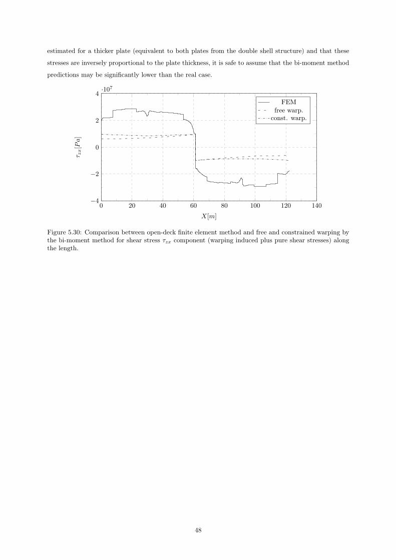
estimated for a thicker plate (equivalent to both plates from the double shell structure) and that these

stresses are inversely proportional to the plate thickness, it is safe to assume that the bi-moment method

predictions may be significantly lower than the real case.

0 20 40 60 80 100 120 140−4

−2

0

2

4·107

X[m]

τ zx[Pa]

FEMfree warp.

const. warp.

Figure 5.30: Comparison between open-deck finite element method and free and constrained warping bythe bi-moment method for shear stress τzx component (warping induced plus pure shear stresses) alongthe length.

48

Chapter 6

Final remarks and further work

The work presented in this dissertation deals with the structural response of an open deck pontoon-like

ship in its elastic domain of material, under vertical and horizontal bending moments, shear forces and

torsional moment, analyzed using both finite element method and simplified approaches. One of its main

focus was to understand if a very simplified thin-wall girder theory application may predict, within an

acceptable range, the expected stress levels under torsion in open deck ships. These expected stress levels

were estimated by finite element method.

The thin-walled girder application uses an idealization of the original structure through a channel-

section with lumped areas, analyzed under the bi-moment method. To create a range of valid stress

values, and since there is no simple methodology to determine the degree of warping constrain, the thin-

walled girder ends were subjected to two different sets of boundary conditions: torsion constrained and

free warping and both torsion and warping constrained.

The conclusion of this study is that the simplified thin-walled girder application, within the predefined

boundary conditions, provides an almost perfect “envelope” for the axial warping stresses verified in the

FE analysis, but its prediction differs in about 194% for the shear warping stresses comparing to the FE

results.

The discrepancy between the warping induced shear stress results of the two different methods, and

in the absence of experimental observations, do not allow to rule any method as either better or worse

since both are built upon many simplifications and constrains. In any way, since the analytical methods

are usually more conservative, the results of the bi-moment method can be regarded as a valid estimation

in an initial design stage, fulfilling thus the purpose of being a reliable prediction method. However, this

is a point to develop and improve in future research, adding some complexity to this otherwise simple

method, by considering the effect of transverse bulkheads as already proposed by some authors.

49

50

Bibliography

[1] J. Vasta, “Lessons learned from full scale structural tests,” Transactions of SNAME, vol. 66, p. 165,

1958.

[2] A. Ostapenko and A. Vaucher, “Ultimate strength of ship hull girders under moment, shear and

torque,” tech. rep., Lehigh University, Fritz Laboratory Reports, 1980.

[3] A. Ostapenko, “Strength of ship hull girders under moment, shear and torque,” in Proceedings of the

SSCSNAME Symposium on Extreme Loads Response, Arlington, USA, pp. 149–166, 1981.

[4] A. Ostapenko and Y. Chen, “Effect of torsion on strength of ship hulls,” tech. rep., Lehigh University,

Fritz Engineering Lab, 1982.

[5] A. Ostapenko and T. R. Moore, “Maximum strength of ship hulls subjected to moment, torque and

shear,” tech. rep., Lehigh University, Fritz Laboratory Reports, 1982.

[6] D. Hong and O. Kim, “Analysis of structural damage of a large ore/coal carrier,” in Ship Technology

and Research Symposium (STAR), 12th, 1987.

[7] J. K. Paik, A. K. Thayamballi, P. T. Pedersen, and Y. I. Park, “Ultimate strength of ship hulls under

torsion,” Ocean Engineering, vol. 28, no. 8, pp. 1097–1133, 2001.

[8] J. K. Paik, “Ultimate longitudinal strength analysis of a double skin tanker by idealized structural

unit method,” in Pro. of SSC/SNAME Symposium, vol. 91, 1991.

[9] J. Paik and A. Thayamballi, “A concise introduction to the idealized structural unit method for

nonlinear analysis of large plated structures and its application,” Thin-walled structures, vol. 41,

no. 4, pp. 329–355, 2003.

[10] H.-H. Sun and C. G. Soares, “An experimental study of ultimate torsional strength of a ship-type

hull girder with a large deck opening,” Marine Structures, vol. 16, no. 1, pp. 51–67, 2003.

[11] P. T. Pedersen, A beam model for the torsional-bending response of ship hulls. Danish Center for

Applied Mathematics and Mechanics [DCAMM], 1982.

[12] P. T. Pedersen, “Torsional response of containerships,” Journal of ship research, vol. 29, no. 3,

pp. 194–205, 1985.

51

[13] R. Pavazza, B. Plazibat, and A. Matoković, “Idealisation of ships with large hatch openings by a

thin-walled rod of open section on many elastic supports,” Thin-walled structures, vol. 32, no. 4,

pp. 305–325, 1998.

[14] R. Pavazza, “Torsion of thin-walled beams of open cross-section with influence of shear,” International

Journal of Mechanical Sciences, vol. 47, no. 7, pp. 1099–1122, 2005.

[15] I. Senjanović and Y. Fan, “On torsional and warping stiffness of thin-walled girders,” Thin-Walled

Structures, vol. 11, no. 3, pp. 233–276, 1991.

[16] I. Senjanovic and Y. Fan, “Pontoon torsional strength analysis related to ships with large deck

openings,” Jornal of Ship Research, vol. 35, no. 4, pp. 339–351, 1991.

[17] I. Senjanović and Y. Fan, “A higher-order theory of thin-walled girders with application to ship

structures,” Computers & Structures, vol. 43, no. 1, pp. 31–52, 1992.

[18] I. Senjanovic and Y. Fan, “A finite element formulation of ship cross-sectional stiffness parameters,”

Brodogradnja, vol. 41, no. 1, pp. 27–36, 1993.

[19] I. Senjanović, T. Senjanović, S. Tomašević, and S. Rudan, “Contribution of transverse bulkheads to

hull stiffness of large container ships,” Brodogradnja, vol. 59, no. 3, pp. 228–238, 2008.

[20] I. Senjanović, S. Tomašević, S. Rudan, and T. Senjanović, “Role of transverse bulkheads in hull

stiffness of large container ships,” Engineering Structures, vol. 30, no. 9, pp. 2492–2509, 2008.

[21] I. Senjanović, S. Rudan, and N. Vladimir, “Influence of shear on the torsion of thin-walled girders,”

Transactions of FAMENA, vol. 33, no. 2, pp. 35–50, 2009.

[22] I. Senjanović, N. Vladimir, and M. Tomić, “Effective stiffness of the engine room structure in large

container ships,” Brodogradnja, vol. 62, no. 1, pp. 15–27, 2011.

[23] I. Senjanovic, N. Vladimir, and M. Tomić, “Investigation of torsion, warping and distortion of large

container ships,” Ocean Systems Engineering, vol. 1, no. 1, pp. 73–93, 2011.

[24] K. Iijima, T. Shigemi, R. Miyake, and A. Kumano, “A practical method for torsional strength

assessment of container ship structures,” Marine structures, vol. 17, no. 5, pp. 355–384, 2004.

[25] E. J. Sapountzakis and V. G. Mokos, “Warping shear stresses in nonuniform torsion by bem,” Com-

putational Mechanics, vol. 30, no. 2, pp. 131–142, 2003.

[26] V. G. Mokos and E. J. Sapountzakis, “Secondary torsional moment deformation effect by bem,”

International Journal of Mechanical Sciences, vol. 53, no. 10, pp. 897–909, 2011.

[27] R. Villavicencio, S. Zhang, and J. Tong, “A study of cross deck effects on warping stresses in large

container ships,” Analysis and Design of Marine Structures V, p. 385, 2015.

[28] M. Shama, Torsion and shear stresses in ships. Springer, 2010.

52

[29] DNV, Rules for the classification of ships. Det Norske Veritas, 2001.

[30] P. A. Seaburg and C. J. Carter, Steel design guide series 9: Torsional analysis of structural steel

members. American Institute of Steel Construction, 2003.

53