Structural Change and Global Trade

Logan T. Lewis Ryan MonarchFederal Reserve Board Federal Reserve Board

Michael Sposi Jing ZhangSouthern Methodist University Federal Reserve Bank of Chicago

November 2020

AbstractServices, which are less traded than goods, rose from 55 percent of world expen-

diture in 1970 to 75 percent in 2015. Using a Ricardian trade model incorporatingendogenous structural change, we quantify how this substantial shift in consumptionhas affected trade. Without structural change, we find that the world trade to GDPratio would be 13 percentage points higher by 2015, about half the boost deliveredfrom declining trade costs. In addition, a world without structural change would havehad about 40 percent greater welfare gains from the trade integration over the past fourdecades. Absent further reductions in trade costs, ongoing structural change impliesthat world trade as a share of GDP would eventually decline. Going forward, higherincome countries gain relatively more from reducing services trade costs than fromreducing goods trade costs.

JEL classifications: F41, L16, O41

Keywords: Globalization, Structural Change, International Trade

The views expressed here should not be interpreted as reflecting the views of the Federal Reserve Board ofGovernors, the Federal Reserve Bank of Chicago, or any other person associated with the Federal ReserveSystem. We thank Diego Comin, Kerem Cosar, Lukasz Drozd, Colin Hottman, Kiminori Matsuyama, MartiMestieri, Sebastian Sotelo, Tomasz Swiecki, Kei-Mu Yi, and two anonymous referees for useful comments.This paper also benefited from audiences at the Chicago Fed, the Federal Reserve Board, the Hong KongUniversity of Science and Technology, the International Monetary Fund, the University of California at SantaCruz, the University of Pittsburgh, the University of Rochester, the University of Western Ontario, the Uni-versity of Wisconsin, and Wayne State University, as well as participants at the 2017 Society for EconomicDynamics Conference, 2017 BNM/IMF Conference on Challenges to Globalization, 2017 EIIT Conference,Spring 2017 Midwest Macroeconomics Meetings, Spring 2017 Midwest International Trade Meetings, 2018AEA Meetings, 2018 SCEIA Meetings, the 2018 Trade Integration and Growth Network (TIGN) Confer-ence, the 2018 Econometric Society Summer Asian Meetings, 2018 NBER SI ITM Meetings, and 2020 AEAMeetings. Victoria Perez-Zetune provided excellent research assistance.

1 Introduction

Since 1970, world trade relative to world income has grown faster than at any other timein history, with the ratio of global trade to GDP more than doubling from about 20 percentto nearly 50 percent by 2015, as shown in the left panel of figure 1. Understanding thistrend of greater “openness" is important because when trade grows more rapidly than pro-duction, economies become more sensitive to changes in trade flows, trade policy and thecomposition of trade.1 In addition, openness is closely related to gains from trade.

Figure 1: Openness and structural change

1970 1980 1990 2000 2010

Year

0.1

0.2

0.3

0.4

0.5

0.6Openness

1970 1980 1990 2000 2010

Year

0

0.2

0.4

0.6

0.8

1Expenditure shares

GoodsServices

1970 1980 1990 2000 2010

Year

0

0.5

1

1.5

2

Sectoral openness

The typical explanation for the rapid growth in the trade to GDP ratio is a declinein trade costs, including tariff reductions, improvements in communications technology,and lower transportation costs. However, another factor affects the long-run movementin openness but has not been studied in the literature: the share of global spending onservices has risen consistently and substantially, shown in the middle panel of figure 1.This fact, often referred to as “structural change", is a well-known foundational componentof economic growth and development. Yet because services are traded substantially lessthan goods (the right panel), structural change has dampened the growth in global opennessand thus also the potential benefits from trade integration.

Considering these three figures together presents a puzzle of sorts: How could tradegrow so quickly while a relatively less-traded sector gained expenditure share? In fact,trade grew spectacularly in spite of the ongoing transition to services in the world econ-omy, meaning structural change prevented even greater increases in trade. This dynamicbecomes apparent when calculating the correlation between the growth rates of opennessand the services expenditure share. For the world, the correlation is −0.75, meaning that

1See, for example, Hoekman (2015) and Irwin (2002).

1

periods of faster openness growth feature a slower-growing service expenditure share. Thisrelationship also exists at the country level.2

We study the joint evolution of international trade flows and structural change since1970 and answer two related questions: (i) How much has structural change restricted thegrowth in global trade openness and, hence, the gains from trade? How does the magnitudeof that restriction compare to the effect of lowering trade barriers over the same period?(ii) What are the implications of future trade liberalization in either goods or services in theface of continued structural change? We find that, by 2015, structural change has held backopenness by 13 percentage points, or about one-third. The magnitude of this novel channelis half as much as declining trade costs have boosted openness over this period. The gainsfrom trade estimated in our model without structural change increase about 40 percentmore compared to our baseline model with structural change. Absent further reductions intrade costs, ongoing structural change implies that trade openness would eventually decline.Moreover, rich countries stand to benefit relatively more from liberalizing services tradethan from liberalizing goods trade, and poor countries, the opposite.

The key insight is that structural change, the result of both price and income effects,determines what we consume, produce, and trade. The data show that the share spenton services increases with real income and with relative services prices, both of which areendogenous to the trade regime. As countries open up to trade, the relative price of servicesand real income both rise, shifting expenditure to services and attenuating the benefits frommore-integrated goods markets.

To analyze the endogenous interaction between structural change and trade patternsover time, we build a two-sector, multi-country, Ricardian trade model, similar to Uy, Yiand Zhang (2013) and Sposi (2019). On the production side, labor and intermediates pro-duce a continuum of varieties in each sector. Countries differ in sectoral productivity andtrade costs, forming the basis for comparative advantage. The evolution of sectoral produc-tivity and bilateral trade costs influences the patterns of production and trade over time. Onthe demand side, nonhomothetic preferences allow for total income and relative prices toshape sectoral expenditure shares, as in Comin, Lashkari and Mestieri (2020).

We calibrate the underlying structural parameters and time-varying processes of themodel to relevant observables in 26 countries and a rest-of-world aggregate from 1970–2015. Using data on sectoral expenditures, sectoral prices, and employment levels, we

2For detailed results see Appendix B.1. When a country featured higher growth in its service expenditureshare, it experienced lower growth in openness, even controlling for its level of income per worker.

2

estimate the key preference parameters, namely the elasticity of substitution between goodsand services and the income elasticity of demand for both goods and services. Serviceshave a higher income elasticity than goods, generating a positive correlation between theservices expenditure share and income. In addition, goods and services are complementsso relatively higher productivity growth in the goods sector induces a lower expenditureshare on goods. As Comin et al. (2020) show, the higher income elasticity of services iscrucial for explaining the trend of higher services expenditure shares seen across countries.Coupling these with input-output coefficients from the World Input-Output Database andbilateral trade data enables us to back out estimates of productivity and trade costs at thesector level from the structural equations of the model.

The fundamental question of this paper is how different the path of trade over the lastfour decades would have been if not accounting for the fact that growth shifts the econ-omy away from goods and towards services. In the baseline model, structural change is anendogenous outcome in response to the exogenous forces of productivity and trade coststhrough the price and income effects. In the counterfactual, we mute movements in ex-penditure shares by setting the price and income elasticities to one while using the sameprocesses of productivity and trade costs as in the baseline model. As a result, the coun-terfactual generates incomes, prices, and sectoral trade shares consistent with those in thebaseline and the data, but different expenditure shares. This counterfactual implies a sub-stantial increase in the global trade-to-expenditure ratio relative to the data—13 percentagepoints, or 28 percent higher than that in reality by 2015. That is, without taking into ac-count structural change, we would have expected substantially more trade growth in recentdecades. For quantitative comparison, we use the model to show that the magnitude of thedecrease in this ratio resulting from structural change is about half the magnitude of theincrease in openness that stemmed from lower trade barriers.

The model incorporating nonhomothetic preferences requires using equivalent varia-

tion to measure the welfare gains from trade.3 Using observed trade integration over thepast four decades, we estimate that the gains from trade relative to autarky have increasedby 5.3 percentage points. This is lower than in a counterfactual world with expenditureshares held fixed from 1970 onwards, in which gains from trade increase by 7.8 percentagepoints. Thus, since structural change holds back goods trade, and goods trade is a majorcontributor to welfare gains, properly accounting for structural change implies lower esti-

3The class of additively non-separable nonhomothetic preferences we use is not within the set discussedby Arkolakis, Costinot, Donaldson and Rodríguez-Clare (2019).

3

mated welfare gains. We also find that relative price changes, rather than income effects,explain most of the difference between the 5.3 and 7.8 percentage point changes.

Projecting our model into the future by assuming constant trade costs and continuedtechnical progress, we demonstrate that openness has peaked and may decline to about 40percent by 2060. Importantly, the projected downward trend in the trade to GDP ratio isdriven by the effects of increased services consumption. At the same time, there is littleevidence that the recent slowdown in international trade growth that started in 2011 is dueto these forces; that is, structural change has been a drag on trade growth for decades, andthe drag has not been stronger in recent years.

To the extent that structural change reflects the efficient, long-run response of expendi-tures and production to asymmetric technological progress and aggregate income growth, itwould not prove prudent to design policies that restrict the expansion of the service sector.Furthermore, trade policy has become increasingly restrained in its ability to further boosttrade in goods, as tariffs are currently low. Modern trade policy could focus on liberalizingtrade in services in order to foster the growth in world trade and to stimulate the benefitstherein. Indeed, we estimate the projected gains from further reductions in trade barriersin either goods or services in the face of continued structural transformation induced bytechnical progress. The benefits from liberalizing services trade complements the risingservices expenditures, particularly when the services sector becomes substantially moreopen. Moreover, rich countries gain relatively more from liberalizing services trade thanfrom liberalizing goods trade, while the opposite is true for poor countries.

This paper contributes to a broad literature on how global trade grows relative to GDP.In an early theoretical contribution, Markusen (1986) includes nonhomothetic preferencesin a trade model to be consistent with empirical evidence of a relationship between incomeand trade volumes. Rose (1991) shows that increases in income and international reservesalong with declining tariff rates help explain the differences in trade growth across coun-tries over three decades. Krugman, Cooper and Srinivasan (1995) analyze the growth inworld trade since World War II and potential consequences for labor markets. Baier andBergstrand (2001) find that income growth explains nearly two-thirds of the increase inglobal trade, while tariffs explain an additional one-quarter. Imbs and Wacziarg (2003)document a U-shaped pattern of specialization as countries become richer; they first diver-sify across industries and only later specialize as they grow. Yi (2003) shows how verticalspecialization—the splitting of production stages across borders—can amplify gross traderelative to value-added trade and help explain the large increases in trade-to-GDP ratios.

4

Our paper provides an additional reason why the trade-to-GDP ratio is an imperfect mea-sure of true openness, and given our projection exercise, a decline in this ratio does notnecessarily reflect a less-open world with increasing protectionism.

A well-established literature documents how international trade and openness affectstructural change. Matsuyama (2009) emphasizes that trade can alter patterns of structuralchange and that using closed-economy models may be insufficient. Uy et al. (2013) findthat rapid productivity growth in South Korea’s manufacturing sector contributed to a risein manufacturing employment share due to improved comparative advantage. In a closedeconomy, the same productivity growth would have produced a decline in the manufactur-ing share. Betts, Giri and Verma (2017) explore the effects of South Korea’s trade policieson structural change, finding that these policies raised the industrial employment share andhastened industrialization in general. Teignier (2018) finds that international trade in agri-cultural goods affected structural change in the United Kingdom even more than in SouthKorea. We show in this paper that structural change may be more consequential for inter-national trade than trade is for explaining structural change in many countries.

More broadly, our findings point to structural change as being an important link betweeninternational trade and economic development. McMillan and Rodrik (2011) find that theeffect of structural change on growth depends on a country’s export pattern, specificallythe degree to which a country exports natural resources. Cravino and Sotelo (2019) showthat structural change originating from greater manufacturing trade increases the skill pre-mium, particularly in developing countries. Sposi (2019) documents how the input-outputstructures of advanced economies are systematically different from those of developingeconomies, which contributes to systematic differences in resource allocations betweenrich and poor countries. Markusen (2013) shows how including nonhomothetic preferencesinto a Hecksher-Ohlin model can help explain why we observe less trade than predicted bymodels without nonhomotheticities.

Some analyses suggest that international trade plays only a small role in explainingstructural change. Kehoe, Ruhl and Steinberg (2017) find that relatively faster growth inmanufacturing productivity was the primary cause for reduced employment in the goods-producing sector in the United States, with a smaller role for trade deficits. Swiecki (2017)also finds differential productivity growth is more important than other mechanisms, in-cluding international trade, in explaining structural change. Nonetheless, even if interna-tional trade only contributes a small portion to structural change, we show that structuralchange plays a large role in the growth of world trade.

5

Nonhomothetic preferences are important in understanding other aspects of interna-tional trade. Fieler (2011) uses nonhomothetic preferences to explain why trade growswith income per capita but not population. Caron, Fally and Markusen (2014) documentsa positive correlation between the income elasticity and skilled labor intensity across sec-tors and demonstrates that this is important for understanding international trade patterns.Simonovska (2015) uses nonhomothetic preferences to explain the empirical pattern thathigher-income countries have higher prices of tradable goods. Matsuyama (2015) and Mat-suyama (2019) show that nonhomothetic preferences combined with home market effectscan lead to high-income countries producing and exporting higher income elasticity goodswithout assuming they have an exogenous comparative advantage in such goods.

The remainder of the paper proceeds as follows. We set up the model in Section 2,describe the data and calibration of the model in Section 3, and present the quantitativeresults in Section 4. We conclude in Section 5.

2 Model

We consider a multi-country, two-sector, Eaton-Kortum trade model of the global econ-omy with nonhomothetic preferences. There are I countries and the two sectors are goods(g) and services (s). Household preferences have non-unitary income and substitution de-mand elasticities. In each sector, there is a continuum of varieties, and production usesboth labor and intermediate inputs. All varieties are tradable, but trade costs vary acrosssectors, country-pairs, and over time. Productivities also differ in initial levels and subse-quent growth rates across sectors and countries. These time-varying forces drive structuralchange. We omit the time subscript in this section for brevity.

2.1 Endowments and Preferences

Labor is mobile across sectors within a country, but immobile across countries. Let Li

denote total labor endowment in country i, which varies over time, and Lik denote laboremployed in sector k. The factor market clearing condition is given by:

Li = Lig +Lis. (1)

The household in country i maximizes the level of aggregate consumption, Ci, which isa function of sectoral consumption Cig and Cis. Aggregate consumption, which is a stand in

6

for the overall utility level, combines sectoral composite goods according to the implicitlydefined function:

∑k=g,s

ω1σ

k

(Ci

Li

) εk(1−σ)σ(

Cik

Li

) σ−1σ

= 1, (2)

where for each sector k ∈ {g,s}, ωk > 0 describe the relative weight of each sector in theaggregate consumption bundle. These preferences, known as “Non-Homothetic ConstantElasticity of Substitution”, are discussed by Hanoch (1975) and are also used by Comin etal. (2020). The elasticity of substitution across sectoral composite goods is σ . If σ > 1,goods and services are substitutes, and if σ < 1, they are complements. Parameter εk

governs the income elasticity of demand for sector k. The sector with a greater εk is aluxury good, which expands in expenditure shares as the income rises, all else equal.

Hanoch (1975) showed that in order for these preferences to be well-behaved, i.e.,monotone and quasi-concave, we require εk > 0 and either (i) 0 < σ < 1 or (ii) σ > 1must hold.4 Given our broad categorization of the two sectors, goods and services are com-plements empirically, so (i) is the relevant case in our context.5 As is usual when dealingwith non-homothetic preferences, one of the income elasticity parameters needs to be nor-malized, since only the difference matters for allocations.6 We normalize εg = 1. Anotherattraction of this normalization is that when εs is set at one, the preferences collapse intothe commonly used homothetic CES preferences in the literature.

Comin et al. (2020) show that this specification of nonhomothetic preferences has twoattractive properties for studying long-run structural change. First, the elasticity of therelative demand for the two sectoral composites with respect to aggregate consumption isconstant at all levels of consumption. This contrasts with Stone-Geary preferences, wherethe elasticity of relative demand goes to zero as income or consumption rises—a predictionat odds with the data both at the macro and micro levels. Second, the elasticity of substitu-

4Our notation differs from Hanoch (1975, p. 403). These conditions are a rewriting of expression (i), withd = σ−1

σand ei = εk.

5For the empirical estimation of σ and εk see section 3.2.6In our notation, C is really utility and the income elasticities are technically elasticities w.r.t. utility levels.

Scaling each sector’s income elasticity by the same proportion is a monotonic transformation of the utilityfunction and only affects cardinal properties of the level of utility. Comin et al. (2020) employ the samepreference structure as we do in a three-sector model and normalize the income elasticity in one sector to 1.Another commonly used class of preferences is “Stone-Geary”, which incorporates income effects throughsector-specific subsistence requirements. With Stone-Geary preferences, the subsistence term is normalizedto zero in at least one sector; see Herrendorf, Rogerson and Valentinyi (2013) and Kongsamut, Rebelo andXie (2001).

7

tion between sectoral composites, given by σ , is constant over income, meaning that thereis no functional relationship between income and substitution elasticities.7

The representative household maximizes aggregate consumption, Ci, in each period bychoosing sectoral consumption levels, Cik, subject to the following budget constraint:

PigCig +PisCis︸ ︷︷ ︸PiCi

+ρiwiLi = wiLi +RLi, (3)

where wi and Pik denote the wage rate and the price of the sector-k composite good, respec-tively, and Pi denotes the cost of aggregate real consumption (i.e., the price of one util whenexpenditures are optimally allocated across goods and services). The household suppliesits labor endowment inelastically and spends its labor income on consumption. A frac-tion ρi of income is sent into a global portfolio, and the portfolio disperses R in lump sumequally across countries on a per-worker basis. ρi varies over time and R is determined byglobal portfolio balance in each period. Therefore, each country lends, on net, ρiwiLi−RLi

to the rest of the world. This aspect enables the model to tractably match aggregate tradeimbalances in the data, as in Caliendo, Parro, Rossi-Hansberg and Sarte (2018).

The first-order conditions imply that sectoral consumption demand satisfies:

Cik = Liωk

(Pik

Pi

)−σ (Ci

Li

)(1−σ)εk+σ

, (4)

The sectoral expenditure shares are thus given by:

eik ≡PikCik

PiCi= ωk

(Pik

Pi

)1−σ (Ci

Li

)(1−σ)(εk−1)

⇔ eis

eig=

ωs

ωg

(Pis

Pig

)1−σ (Ci

Li

)(1−σ)(εs−εg)

(5)

and the average cost of real consumption is given by:

Pi =

[∑

k=g,sωkP1−σ

ik

(Ci

Li

)(1−σ)(εk−1)] 1

1−σ

. (6)

Thus, the elasticity of substitution between sectors and the sectoral elasticity of incomegovern how relative price and real income per worker shape the sectoral expenditure shares.Specifically, when σ < 1, a rising sectoral relative price pushes up the expenditure sharein that sector, and vice versa. When sectoral income elasticities differ, i.e., εs− εg > 0, the

7This is a key difference from the preferences used in Fajgelbaum and Khandelwal (2016) and Hottmanand Monarch (2018), whose frameworks could be used to ask a similar question to ours.

8

service sector’s expenditure share also rises with consumption per worker.

2.2 Technology and Market Structure

There is a continuum of varieties, z ∈ [0,1], in both the goods (g) and services (s) sectors.The sectoral composite good, Qik, is an aggregate of the individual varieties Qik(z):

Qik =

(∫ 1

0Qik(z)

η−1η dz

) η

η−1

,

where the elasticity of substitution across varieties within a sector is η > 0. Each variety zis either produced locally or imported from abroad. The composite sectoral goods are usedin domestic final consumption and domestic production as intermediate inputs:

Qik =Cik + ∑n=g,s

Mink,

where Mink is the intermediate input of composite good k in the production of sector n.Each country possesses technologies for producing all the varieties in both sectors.

Production requires labor and intermediate inputs as in Levchenko and Zhang (2016). Theproduction function for variety z ∈ [0,1] in sector k ∈ {g,s} of country i is:

Yik(z) = Aik(z)(TikLik(z))λik[Πn=g,sM

γiknikn (z)

]1−λik , (7)

where λik denotes the country-specific value-added share in production, and γikn denotesthe country-specific share of intermediate inputs sourced from sector n; these parametersvary over time to track changes in input-output relationships. Yik(z) denotes output, Lik(z)

denotes labor input, and Mikn(z) denotes sector-n composite goods used as intermediates inthe production of the sector k variety z. Tik is the time-varying, exogenous productivity ofvarieties in sector k and scales value added equally across all varieties. Aik(z)is a variety-specific productivity level that scales gross output, given by the realization of a randomvariable drawn from the cumulative distribution function F(a) = Pr[A ≤ a]. FollowingEaton and Kortum (2002), we assume that F(a) is a Fréchet distribution: e−a−θk . The largerθk is, the lower the heterogeneity, or variance, in Aik(z) is.8 The parameters governing thedistribution of idiosyncratic productivity draws are invariant across countries but differentacross sectors. We assume that the productivity is drawn each period.9

8Ak(z) has geometric mean eγ

θk and its log has a standard deviation π

θk√

6, where γ is Euler’s constant.

9Alternatively, we could assume that the productivity is drawn once in the initial period, and as the T ’s

9

Total sectoral labor, input usage, and production in sector k in country i are the aggre-gates of the variety-level components taken over the set of varieties produced, Vik:

Lik =∫

Vik

Lik (z)dz; Mikn =∫

Vik

Mikn (z)dz; Yik =∫

Vik

Yik (z)dz.

Markets are perfectly competitive; prices are determined by marginal costs of production.The cost of an input bundle in sector k is:

vik = Bikwλiki

(Πn=g,s (Pin)

γikn)1−λik ,

where Bik = λ−λikik ((1− λik)Πn=g,sγ

−γiknikn )λik−1. The cost of an input bundle is the same

within a sector, but varies across sectors given different input shares.

2.3 Trade

When varieties are shipped abroad, they incur trade costs, including transportation costs,information barriers, and other barriers to trade. We model these costs as exogenous icebergcosts, which vary over time to track the pattern of bilateral trade. Specifically, if one unitof variety z is shipped from country j, then 1

τi jmunits arrive in country i. We assume that

trade costs within a country are zero, i.e., τiig = τiis = 1. This means that the price at whichcountry j can supply variety z in sector k to country i equals pi jk(z) =

τi jkv jk

Aik(z)Tλk

ik

. Since

buyers will purchase from the cheapest source, the actual price for this variety in country i

is pik(z) = min{

pi jk(z)}I

j=1.Under the Fréchet distribution of productivities, Eaton and Kortum (2002) show that

the price of composite good k ∈ {g,s} in country i is:

Pik = Γk

[I

∑j=1

(T−λ jk

jk v jkτi jk

)−θk

]− 1θk

, (8)

where the constant Γk = Γ(1− η−1θk

)1

1−η denotes the Gamma function, and the summationterm on the right-hand side summarizes country i’s access to global production technologiesin sector k scaled by the relevant unit costs of inputs and trade costs.10

The share of country i’s expenditure on sector-k goods from country j, πi jk, equals the

change over time, the productivity relative to T remains constant.10We assume η−1< θk to have a well-defined price index. Under this assumption, the parameter η , which

governs the elasticity of substitution across goods within a sector, can be ignored because it appears only inthe constant term Γ.

10

probability of country i importing sector-k goods from country j, and is given by:

πi jk =

(T−λ jk

jk v jkτi jk

)−θk

∑Is=1

(T−λsk

sk vskτisk

)−θk. (9)

Equation (9) shows how a higher average productivity, a lower unit cost of input bundles,and a lower trade cost in country j translates into a greater import share by country i.

2.4 Equilibrium

Combining the goods and factor market clearing conditions and demand equations with theequations for the consumption of the composite good, trade shares, prices, and the globalportfolio balance yields a set of conditions that fully characterize the equilibrium of themodel. Table 1 collects these conditions. Equations (D1)-(D3) describe the householddemand side. (D1) provides the optimal condition for sectoral consumption. (D2) specifiesthe aggregate price index given the preferences. (D3) is the budget constraint.

Table 1: Equilibrium conditions

D1 Cik = Liωk

(PikPi

)−σ (CiLi

)(1−σ)εk+σ

∀i,k

D2 Pi =

[∑k=g,s ωkP1−σ

ik

(CiLi

)(1−σ)(εk−1)] 1

1−σ

∀i

D3 PiCi +ρiwiLi = wiLi +RLi ∀i

S1 πi jk =

(T−λ jkjk ν jkτi jk

)−θk

∑I`=1

(T−λ`k`k ν`kτi`k

)−θk∀i, j,k

S2 νik = Bikwλiki ∏n∈{g,s}P(1−λik)γikn

in ∀i,k

S3 Pik = Γk

(∑

Ij=1

(T−λ jkjk ν jkτi jk

)−θ)− 1

θ

∀i,k

S4 wiLik = λikPikYik ∀i,kS5 PinMikn = (1−λik)γiknPikYik ∀i,k,nS6 Qik =Cik +∑n∈{g,s}Mink ∀i,kS7 ∑k∈{g,s}PikYik−∑k∈{g,s}PikQik = ρiwiLi−RLi ∀i

G1 ∑Ii=1 ρiwiLi = R∑

Ii=1 Li

G2 PikYik = ∑Ij=1 PjkQ jkπ jik ∀i,k

Equations (S1)-(S7) are from the supply side. (S1) gives bilateral import shares in totalabsorption at the sector level. (S2) specifies sectoral input costs, and (S3) gives sectoral

11

prices. (S4) and (S5) state the optimal value added and intermediate input usages impliedby the Cobb-Douglas production function. (S6) links sectoral absorption with final demandand intermediate input demand. (S7) is the resource constraint at the country level.

Equations (G1)-(G2) are from the global market clearing conditions. Equation (G1)specifies net transfers across countries are zero globally. Equation (G2) links a country’stotal output in a sector with the sum of demand from all countries. Together, these condi-tions imply that all labor markets clear.

We define a competitive equilibrium of our model economy with the exogenous time-varying processes for every country: labor endowment {Li}, trade costs {τi jg,τi js}I

i, j=1,productivity {Tig,Tis}, and contribution shares to the global portfolio {ρi}; time-varyingstructural parameters for every country {λik,γikn}; and time-invariant structural parameters{σ ,εk,ωk,θk}k=g,s as follows.

Definition 1. A competitive equilibrium is a sequence of output and factor prices {wi, Pig,Pis, Pi}I

i=1, allocations {Lig, Lis, Migg, Migs, Misg, Miss, Qig, Qis, Yig, Yis, Cig, Cis, Ci}Ii=1,

transfers from the global portfolio, R, and trade shares {πi jg, πi js}Ii, j=1, such that each

condition in table 1 holds.

2.5 Gains from Trade

In existing multisector trade models that feature homothetic preferences like CES andCobb-Douglas, the gains from trade are equivalent to changes in real income or aggre-gate consumption from autarky to trade, and as shown by Costinot and Rodríguez-Clare(2014), there is typically a sufficient statistic for calculating this change. Unfortunately, thestructure of the non-homothetic CES preferences used in our model means that changes inreal income or consumption are not appropriate for quantitative applications, complicatingthe welfare calculation. Instead, we rely on the concept of the equivalent variation to com-pare the equilibrium allocation in both trade and autarky.11 This measure is invariant to anymonotonic transformation of the utility function, i.e., the normalization of εg.

The calculation begins by considering two equilibrium states characterized by differ-ent real incomes and sector prices: the trade equilibrium summarized by (wi,Pig,Pis) andthe autarky equilibrium summarized by (wAUT

i ,PAUTig ,PAUT

is ). These are the equilibriumoutcomes of the baseline model and a counterfactual where the trade costs are set to a pro-

11Nigai (2016) uses the equivalent variation concept to measure heterogeneous gains from trade acrosshouseholds with non-homothetic preferences.

12

hibitively high level, respectively. The welfare changes between the trade regime and theautarky regime for any country i can be expressed using equivalent variation. Equivalentvariation measures the amount of extra income that country i requires in order to obtain theutility level possible in autarky, while facing prices in the trade regime:

EVi = e(Pig,Pis,uAUT )− e(Pig,Pis,u),

where e(·) is the expenditure function, and u= v(wi,Pig,Pis) and uAUT = v(wAUTi ,PAUT

ig ,PAUTis )

are the utility levels for the indirect utility function v(·) evaluated at the two equilibria. Tomatch the literature, we define the gains from trade as the lost income that comes frommoving to the lower utility level in autarky, taken as a fraction of initial income:

GFTi =e(Pig,Pis,u)− e(Pig,Pis,uAUT )

e(Pig,Pis,u). (10)

To take this definition to our model, we derive the indirect utility function and expendi-ture functions. For a country i with a per-capita income level wi and prices (Pig,Pis) underthe trade regime, equilibrium conditions (D2) and (D3) in Table 1 imply the indirect utility(per capita) function v(wi,Pig,Pis) takes the implicit form:

∑k

ωkP1−σ

ik v(wi,Pig,Pis)(1−σ)εk = w1−σ

i . (11)

In turn, expenditure minimization yields the expenditure function e(Pig,Pis,u) as:

e(Pg,Ps,u) =

(∑k

ωkP1−σ

ik u(1−σ)εk

) 11−σ

. (12)

Plugging in the optimal consumption bundle consistent with the model solution as well asa version solved with infinite trade costs will thus permit the calculation of welfare gains.

Importantly, this definition nests the standard method of calculating welfare gains.Since setting εk = 1 for all k produces standard CES preferences, gains from trade underequation (10) are:

GFTi = 1−

(∑k ωσ

k P1−σ

ik

∑k ωσ

k PAUTik

1−σ

) 11−σ wAUT

iwi

= 1− wAUTi /PAUT

iwi/Pi

. (13)

Thus, the gains from trade for homothetic preferences are simply the change in real incomefrom trade to autarky.

13

3 Data and Calibration

In this section, we calibrate the model to set up the stage for the quantitative counterfactu-als and the projection analysis in the next section. Specifically, we calibrate the exogenousprocesses and the parameters in the model to match the following data. Preference parame-ters (σ , εg, εs, ωg, ωs) are estimated using panel data on sectoral prices, expenditure shares,and total expenditure per worker. The trade elasticity, θk, is taken from the literature. Tradeimbalances, ρit , and labor endowment, Lit , are set to match data on trade deficits and totalnumber of employees. Production coefficients λikt and γiknt are constructed using the input-output data. Processes for sectoral trade costs, τi jkt , and productivity, Tikt , are constructedto match data on bilateral trade shares and expenditure shares at the sector level.

We first discuss main data sources in the first subsection, and then describe the calibra-tion procedures together with remaining data sources in the next three subsections. Withthe calibrated parameters, we solve the baseline model for each year t = 1970, . . . ,2015.In the last subsection, we check the model fit by comparing non-targeted moments in themodel with those in the data.

3.1 Data

We begin by more formally laying out the key concepts in our analysis and their relationto the data. Expenditure refers to final demand: consumption, investment, and governmentspending. Structural change refers to changes in the expenditure of goods and servicesas a share of total expenditure over time. Openness is defined as total trade (imports plusexports) as a share of expenditure, with sectoral openness defined analogously at the sector(either goods or services) level. In UN nomenclature, the goods sector consists of “agri-culture, hunting, forestry, fishing” and “mining, manufacturing, utilities,” while servicesincludes “construction,” “wholesale, retail trade, restaurants, and hotels,” “transport, stor-age, and communication,” and “other activities”.

We gather data for 26 countries and a rest-of-world aggregate over the period 1970–2015.12 The trade data comes from two sources. Bilateral trade in goods for 1995–2014come from the World-Input-Output Database (WIOD). The 2013 release covers 1995–2011, while the 2016 release covers 2000–2014. For the remaining years, we splice country-level goods trade data from the IMF Directions of Trade Statistics Database.13 Trade in

12The full list of countries is listed in Appendix A.1.13For pre-1995 trade data, we use annual changes from the data source to extrapolate from average 1995–

14

services is measured less reliably in WIOD, so we take country-level service imports fromthe World Development Indicators (WDI) for all years 1970–2015. The WDI does not re-port bilateral trade in services, so we construct these bilateral flows using bilateral importshares from WIOD for 1995–2014. Prior to 1995, we assume that each bilateral shares forservices equals its average from 1995–1997. This particular approach is not critical be-cause the volume of service trade is small prior to 1995 and the bilateral share distributionis less important then the overall trade volume. We do the same for 2015 based on average2012–2014 values.

Sectoral expenditures are constructed using the identity that sectoral absorption (i.e.,gross output plus imports minus exports) must equal the sum of sectoral expenditures andintermediate expenditures on that sector. We first obtain sectoral output by grossing upsectoral value-added data using gross-output-to-value-added ratios in WIOD.14 We thenadjust sectoral gross output for sectoral imports and exports to build sectoral absorption.Finally, we use intermediate input coefficients to separate intermediate expenditure fromabsorption to obtain final expenditure.15 The details are outlined in Appendix A.1.16

3.2 Preference parameters

To estimate the preferences parameters (σ , εg, εs, ωg, ωs), we collect data on sectoralprices Pik, sectoral expenditure PikCik = Eik, aggregate expenditure, PiCi = ∑k Eik, and em-ployment levels, Li. The construction of sectoral expenditure data is discussed in section3.1. For sectoral prices, we use the UN Main Aggregates Database and the GGDC Pro-ductivity Level Database “2005 Benchmark" from Inklaar and Timmer (2014). Aggregateemployment comes from the Penn World Table and corresponds to “number of personsengaged”. Details of data construction and data sources are provided in Appendix A.1.

We structurally estimate the elasticities of both income and price channels by mini-mizing the distance between the observed sectoral expenditures and those implied by themodel given the observed prices. One complication is that we rely on the model to inferutility, or real aggregate consumption Ci, since there is no direct empirical counterpart to it.

1997 values in WIOD. We do the same for post-2014 data based on average 2012–2014 values.14Some years require imputing country-level gross-output-to-value-added ratios, where our imputation

procedure is based on estimating a relationship between value-added-to-gross-output ratios and income percapita, with country and time fixed effects. Details are available upon request.

15These input-output coefficients also need to be imputed for some country years. Full details are presentedin the Appendix, though the results are not sensitive to our choice of imputation.

16A stylized depiction of this calculation is in figure B.5 in the Appendix.

15

Formally, the preference parameters are estimated by solving a constrained nonlinear leastsquares problem:

min(σ ,εs)

T

∑t=1

I

∑i=1

(ωs

ωg

)(Pist

Pigt

)1−σ (Cit

Lit

)(1−σ)(εs−εg)

−

(Eist

Eigt

)2

(14)

s.t. εg = 1 (15)

ωg +ωs = 1 (16)

Eigt + Eist

Lit=

(∑

k=g,sωkP1−σ

ikt

(Cit

Lit

)(1−σ)εk) 1

1−σ

,∀(i, t), (17)

where observables are denoted using a “hat”. Equation (15) normalizes the income elas-ticity for goods to one. As in Comin et al. (2020), this normalization has no influence onequilibrium allocations; instead different values of εg reflect monotonic transformations ofthe same utility function. Equation (16) normalizes the sum of ωg and ωs to one withoutloss of generality. We have flexibility in setting ωs by changing the units of relative prices.Specifically, we normalize relative prices such that ωs = 0.55, the global expenditure shareon services in 1970. Equation (17) implicitly specifies utility Cit obtained with the expen-diture per capita, Eig+Eis

Litand sectoral prices Pikt . It is derived by multiplying the price index

in equation (D2) by CiLi

on both sides. Since the expenditures per capita and sectoral pricesare observed, we can infer the real aggregate consumption (utility) implicitly.

For estimation purposes, we drop the year 2015 and drop the rest-of-world aggregate,leaving us with 26 countries and 45 years. We solve the minimization problem as follows.Start by making a guess for (σ ,εs). Given this guess, we exploit aggregate expenditure andsectoral price data to impute the aggregate consumption index, Cit , for each country in everyyear using constraint (17), which is a simple nonlinear equation with one unknown. Giventhe imputed consumption indexes we then exploit data on sectoral prices and expendituresand use nonlinear least squares on the objective function (14) to obtain updated estimatesof (σ ,εs). With the updated estimates of the preference parameters in hand, we revisitequation (17) and impute updated consumption indexes and, in turn, obtain new estimatesof the preference parameters by minimizing (14). We continue the iterative procedure untilwe converge to a fixed point in the preference parameter space. Finally, we bootstrap theconfidence interval for the estimates.17

17We bootstrap the standard errors by drawing country-time pairs with replacement to obtain the samenumber of observations in each bootstrapped series. We report the 2.5 and 97.5 percentiles of 1000 boot-

16

Table 2 reports the estimation results. Using annual data, we obtain point estimatesσ = 0.16 and εs = 1.73, reported in the left columns. Both parameters are statisticallysignificantly different from one, implying the strong presence of both income and priceeffects for accounting for the structural patterns of expenditure shares. We also conductthe estimation on the non-overlapping, five-year averages of the expenditure and price datato smooth out the short-run variations, which is not the focus of our long-run structuralchange process. The results are reported in the right columns of the table. The estimatedparameter values are almost identical to those in the baseline estimation. In the estimationprocess, we obtain estimates of the aggregate consumption index, Cit , which will be usedto calibrate productivity levels in an internally consistent manner later on.

Table 2: Estimated Preferences Parameter Values

Baseline 5-year averagesVariable Estimate 95% C.I. Estimate 95% C.I.σ 0.16 (0.08,0.23) 0.16 (0.08,0.24)εs 1.73 (1.64,1.86) 1.75 (1.63,1.87)Number of observations 1170 134

Note: The 95 percent confidence intervals are constructed using a naive bootstrap with 1000 repetitions. Esti-mates reported under the “5-year averages” column are based on data averaged over 1970–1974, 1975–1979,. . . 2000–2014. We drop the year 2015 and we also drop the rest-of-world aggregate from both estimations.

Our estimates of the preference elasticities are consistent with the regularity conditionsspecified in Section 3.1, namely 0 < σ < 1 and εk > 0 for all k. While estimation ofdemand functions may suffer from endogeneity problems, our estimates are remarkablysimilar to those obtained by Comin et al. (2020) using Consumer Expenditure Survey dataat the household level, including instrumenting for household consumption. In addition,their three-sector estimates using cross-country panel data on sectoral employment andvalue added shares are broadly consistent with our two-sector estimates using cross-countrypanel data on expenditure shares.18 Specifically, goods and services are complements, andservices have a higher income elasticity than goods. The structural estimates are also veryclose to the reduced form estimates using OLS, detailed in Appendix A.2.

strapped replications.18Comin et al. (2020) estimate a wide range of elasticities using a three sector model—agriculture, manu-

facturing, and services—using data that goes back to 1947 and includes 37 countries. We conduct robustnessin Appendix B.3 with respect to these elasticities.

17

3.3 Parameters directly from the literature and the data

We set the dispersion parameter of productivity draws in the goods sector, θg, at 4, follow-ing Simonovska and Waugh (2014). There is no reliable estimate of the trade elasticity forservices, so we set θs = 4 as well. We conduct sensitivity analysis for a smaller θs of 2.5in Appendix B.3; the main results are robust. The elasticity of substitution between vari-eties in the composite good, η , plays no quantitative role in the model other than satisfying1+(1−η)/θ > 0; we set this value at 2. The upper panel of Table 3 summarizes theseparameter values.

The country-specific, time-varying production parameters γiknt and λikt are constructedby condensing multi-sector, input-output tables to a two-sector input-output construct.Specifically, λikt is the ratio of value added to total production in sector k, while the γiknt isthe share of sector k intermediate spending that is sourced from sector n. The World Input-Output Database (WIOD) provides country-level data annually from 1995-2014. Prior to1995, we make use of country-specific input-output tables for 11 countries from multiplesources, covering various years depending on the country, resulting in an unbalanced panelof input-output data from 1970-2014 (see Appendix A.1 for more details). We imputethe shares for missing country-year observations by (i) estimating a relationship betweeneach share and GDP per worker in our unbalanced panel and (ii) using the estimates andobserved GDP per worker to fill in the missing values.

While these production shares vary significantly across countries, they change onlymildly over time. Moreover, there are notable patterns that hold across countries. First,production of services is more value-added intensive than production of goods. The lowerpanel of table 3 indicates that, on average, 59 percent of total service production compen-sates value-added factors, compared to 38 percent in goods. Second, inputs from goodssectors account for 67 of intermediate expenditures by the goods sector. That is, goodsproduction is goods-intensive. Similarly, services production is service intensive: inputsfrom the service sector account for 69 percent of intermediate expenditures by the servicesector. Still, cross-sector linkages are relatively strong: roughly one-third of intermediateinputs in each sector is sourced from the other sector.

The parameters ρit are calibrated to match each country’s ratio of net exports to GDP.In the model, the ratio of net exports to GDP in country i at time t is ρitwitLit−RtLit

witLit. In

the calibration, we let Rt = 0 and simply set ρit =NXit

GDPit. So long as net exports sum to

zero across countries (as in our data), the global portfolio is balanced. In the counterfactualanalysis, the endogenous term Rt adjusts to ensure that the global portfolio balances period-

18

Table 3: Parameter values

Preference parametersσ Elasticity of substitution b/w sectors 0.16εg Elasticity of income in goods 1εs Elasticity of income in services 1.73ωg Preference weight on goods 0.45ωs Preference weight on services 0.55

Production parametersθg Trade elasticity in goods sector 4θs Trade elasticity in service sector 4η Elasticity of substitution b/w varieties in composite good 2

Input-Output parameters (cross-country, cross-time averages)λg Ratio of value added to gross output in goods sector 0.38λs Ratio of value added to gross output in service sector 0.59γgg Good’s share in intermediates used by goods sector 0.67γsg Good’s share in intermediates used by service sector 0.31

by-period: Rt ∑Ii=1 Lit = ∑

Ii=1 ρitwitLit .

3.4 Technology and Trade Costs

We recover the exogenous productivity terms, Tik, and trade costs, τi jk, by exploiting struc-tural relationships from our model in order to match the panel data on sectoral expendituresand bilateral trade flows. In each year, we calibrate 2I productivity parameters and 2I(I−1)trade cost parameters to match 2I sectoral expenditures and 2I(I−1) bilateral trade flows.One major benefit of this approach is that we automatically match the observed sectoralvalue added shares exactly given the matched expenditure shares, trade shares and input-output shares. We do so in two steps. First, we use the estimated preference parameters andthe aggregate consumption index Cit from section 3.2 to impute sectoral prices {Pig,Pis} thatare consistent with the observed sectoral expenditures. Second, we use two key structuralrelationships to provide identification for productivity and trade costs:

T λikik =

νik

Γ−1k Pik (πiik)

− 1θk

=Bikwλik

i ∏n∈{g,s}P(1−λik)γiknin

Γ−1k Pik (πiik)

− 1θk

, (18)

τi jk =

(πi jk

π j jk

)− 1θk(

Pik

Pjk

). (19)

19

Both structural relationships are derived by manipulating equations (8) and (9). Our pro-cedure is similar to that of Swiecki (2017), but incorporates input-output linkages as inLevchenko and Zhang (2016) and Sposi (2019). In this step, we also need data on wageswi to construct unit costs.

Measurement of sectoral productivity takes into account differences between input costsand output prices. Holding fixed the unit costs of inputs, the model assigns a high produc-tivity to a country with a low price, meaning that inputs are converted to output at an effi-cient rate. It also takes into account the home trade share, which reflects the selection effectin Ricardian trade models. Measurement of the trade costs takes into account cross-countryprice differences and the bilateral trade shares. Holding fixed the imputed price differencebetween countries i and j, if country i imports a large share from country j relative to whatj sources from itself, the inferred trade barrier is low.

One potential concern of this calibration strategy is that the imputed prices do not matchthe observed prices, because preference parameters are set constant across countries andover time. However, the differences between the imputed and observed prices are min-imized in the preferences estimation, which is further illustrated in the evaluation of themodel fit in section 3.5. An alternative calibration strategy is to directly use the observedsectoral prices and trade flows in equation (18) and (19) so that the model reproduces theprices. We conduct the quantitative analysis using this alternative calibration and our mainresults are robust.19 One downside of this strategy is that it will not match the observed ex-penditure shares and value added shares exactly. Furthermore, services prices in particulartend to be measured with more error and noise than expenditures.

The estimated sectoral productivity and trade costs are illustrated in figure 2. The up-per panel plots the log of the fundamental productivity levels, Tik, of the median country(solid lines), the 25th percentile country and the 75th percentile country (dashed lines) atthe sector level in each year. As shown in the figure, productivity grows faster in goodsthan in services. Specifically, over the sample period, on average the median fundamentalproductivity series grows by 3.3 percent per year in the goods sector and by 0.1 percent inthe services sector. The cross-country productivity dispersion is fairly stable over time inboth sectors.

19Results are available upon request.

20

Figure 2: Calibrated global productivity and trade costs

1970 1980 1990 2000 2010-1

0

1

2

3Goods productivity

1970 1980 1990 2000 2010-1

0

1

2

3Services productivity

75th percentile50th percentile25th percentile

1970 1980 1990 2000 20100

5

10

15

20Goods barriers

1970 1980 1990 2000 20100

5

10

15

20Services barriers

Note: Productivity plots in logs for each sector are normalized by the 1970 value of the median seriesof that sector. Trade barrier plots report the net trade cost, τ−1.

To gauge how reasonable these fundamental productivity series are, we compare themodel implied labor productivity with that in the data. In a model with selection dueto international trade, the model-implied labor productivity is in general higher than thefundamental productivity. The model-implied sectoral labor productivity is consistent withthe data. On average, median labor productivity for goods grows by 3.8 percent per year inthe model, compared to 4 percent in the data. For services, the median labor productivitygrows by 1.7 percent per year in the model, compared to 0.16 percent in the data. Thecalibrated model slightly misses sectoral productivity growth, because the calibration doesnot target sectoral employment or sectoral prices in the data.

The lower panel of figure 2 plots the net trade barriers, τi jk−1, for goods and servicesover time. Again, the solid line is for the median level, and the dashed lines are for the25th and the 75th percentiles. As illustrated in the figure, trade costs for both goods andservices decline over time, and trade costs in services are generally higher than those ingoods. Also, the cross-country dispersion of the trade barriers declines substantially inboth sectors over time. Furthermore, the trade barriers decline faster in the goods sectorthan in the services sector. Over the sample period, the median trade barriers decline byabout 50 percent (from 4.7 to 2.4) for goods, but only by about 25 percent (from 6.5 to 4.8)

21

for services. The magnitudes of our estimated trade barriers for the goods sector are similarto those in Levchenko and Zhang (2016), and other papers in the literature.

3.5 Model Fit

Our calibration procedure ensures that the model fits data on sectoral value added, sectoralgross output, sectoral absorption, sectoral bilateral trade flows, sectoral expenditures, input-output linkages, and total employment. We now check the fit of the model on observedmoments that are not targeted directly by the calibration.

The first two sets of untargeted moments are the sectoral prices, illustrated in the leftand middle panels of figure 3. Each point corresponds to the price for a country-year withthe model value on the y-axis and the data value on the x-axis. Of course, the points arelimited by the incomplete coverage of the price data. All prices are taken relative to theU.S. in 2011 and in log values. The prices fit the data reasonably well; the correlationbetween the model and the data is 0.90 for goods prices and is 0.92 for services prices.20

Figure 3: Relative prices and services labor shares: model versus data

-2 -1 0 1 2

Data

-2

-1

0

1

2

Mod

el

Goods Prices

45o

-2 -1 0 1 2

Data

-2

-1

0

1

2Services Prices

0 0.5 1

Data

0

0.2

0.4

0.6

0.8

1Services employment share

Note: Prices are in logs, normalized relative to the U.S. in 2011. Employment share depicts the number of workers engaged in servicesas a share of the entire workforce.

The second moment we check is the sectoral employment share. In the right panel offigure 3, we plot the services employment shares in the data against those implied by thebaseline model. The baseline model succeeds in replicating the employment shares across

20The fit for prices is strong in both both within countries (over time) and across countries. The fit withincountries is computed by indexing each country’s price to 1 in 1970; for goods the correlation is 0.92 and forservices is 0.87. The fit across countries is computed by normalizing each country’s price relative to the U.S.in each year; the correlation for goods is 0.83 and for services is 0.93.

22

sectors for all sample countries over time. The correlation between the model and the datais 0.92.

The calibration successfully matches the targeted moments in the data. Moreover, thecalibrated model fits well on the above data moments that are not directly targeted by thecalibration. Thus, the baseline model closely maps into the relevant data for our analysisand serves as the baseline for the counterfactual analysis in the next section.

4 Counterfactuals

This section quantitatively assesses the dampening effect of structural change on globaltrade volumes in the past four decades by conducting counterfactuals using the calibratedmodel. We find that the magnitude of this dampening effect from structural change is abouthalf as large as the boosting effect of declining trade costs on openness in this period. Wealso highlight the importance of structural change on the measurement of the gains fromtrade. Finally, we project structural change into the future and consider the implications foropenness and welfare for liberalizing trade in either goods or in services.

4.1 Global Trade in the Absence of Structural Change

To examine the implications on global trade flows from structural change, we construct acounterfactual in which structural change is absent by restricting expenditure shares to beconstant over time. There are two ways to turn off movements in expenditure shares. Oneis to mute the mechanisms that generate endogenous expenditure shares by setting boththe price and income elasticities to one. Another is to set the exogenous forces constantover time or to alter the exogenous forces in a way to offset the income and price effectsexactly. If we were to take the latter approach, we would generate counterfactual processesfor prices and income as well as trade shares. The simplest case of this approach is to setthe exogenous forces constant over time, which implies time series of all variables constantat their respective 1970 levels. A more complex way is to calibrate productivity and tradecosts across countries so that the income and price effects completely offset each other.Clearly, there does not exist a unique calibration to achieve this. For example, one way isfor productivity to grow faster in services than in goods if countries’ incomes grow overtime. Another is for countries’ incomes to decrease over time if productivity declines fasterin services than in goods. Any of these scenarios would alter the patterns of income, prices,

23

and sectoral trade openness away from the baseline model and the data, which makes itchallenging to isolate the impact of structural change alone.

For the counterfactual analysis, we take the first approach and adopt Cobb-Douglaspreferences to remove structural change:

Ci = ∏k∈{g,s}

Cω ′ikik . (20)

With the Cobb-Douglas specification, the income elasticities are one for both sectors andthe substitution elasticity is also one across the two sectors. Consequently, expenditureshares across sectors are invariant to economic conditions and constant over time. That is,we choose values for ω ′ik = eik0 so that in 1970, the sectoral expenditure shares are identicalto those in the baseline model. We retain the same asymmetric productivity and trade costchanges backed out from the baseline model calibration, leaving those same exogenousforces to affect comparative advantage and resource allocations over time. By doing so,we isolate the impact of structural change in expenditure shares on aggregate openness.Another benefit of this counterfactual is that it helps us understand how the commonlyadopted Cobb-Douglas utility functions, which are grossly inconsistent with the structuralchange patterns in sectoral expenditures shares, impact the predictions of quantitative trademodels on trade flows and gains from trade.

All underlying processes in the counterfactual are identical to those in the baseline.Specifically in the counterfactual, we assume all other parameters and time varying pro-cesses for Tik, τi jk, and Li are unchanged from the baseline, except that the preferenceparameters {σ ,εg,εs,ωk} in the baseline are set to {1,1,1,ω ′ik} in the counterfactual exper-iment. We compute the equilibrium for the counterfactual experiment and analyze how theabsence of structural change impacts global trade flows. Our solution procedure is basedon Alvarez and Lucas (2007). Start with an initial guess for the vector of wages. Givenwages, recover all remaining prices and quantities across countries using optimality con-ditions and market clearing conditions, excluding the trade balance condition. Then usedepartures from the trade balance condition to update the wages. Iterate on wages until thetrade balance condition holds. Details are available in appendix B.2.

We now present the implications for global trade flows.21 Figure 4 compares openness

21The goods share in total expenditure falls from about 45 in 1970 percent to 25 percent in 2015 in boththe data and the baseline model. In the counterfactual, the goods expenditure share is held fixed at the 1970values, country-by-country. The slight rise since 2002 is driven by the increasing weight of China and Indiain the world economy, both of which have larger expenditure shares in goods compared to the developed

24

between the baseline model (solid line) and counterfactual (dashed line), and it shows thatglobal trade would have been much higher had structural change not occurred. By 2015, thecounterfactual yields 61 percent openness compared with 48 percent in the data/baseline.22

Figure 4: Openness: baseline and counterfactuals

1970 1975 1980 1985 1990 1995 2000 2005 2010 20150

0.2

0.4

0.6

0.8

1Baseline/DataFixed expenditure shares

4.1.1 Quantitative mechanisms

A key benefit of the general equilibrium structure is its ability to deliver an alternate pathfor sectoral openness that responds to the same forces that drive structural change. Theleft two panels of Figure 5 compares sectoral openness in the model counterfactual withthe observed sectoral openness. In the model counterfactual, goods openness (the ratioof goods trade to goods expenditure) is about 40 percentage points lower relative to thebaseline in 2015, while services openness is about 4 percentage points higher.

To understand how sectoral openness endogenously responds to changes in expenditureshares, we decompose sectoral trade openness into two terms: (i) the ratio of trade toabsorption and (ii) the ratio of absorption to expenditure:

Tradekt

Expkt=

(Tradekt

Abskt

)×(

Abskt

Expkt

). (21)

Through endogenous general equilibrium effects, changing sectoral demand might changerelative wages across countries, and thus the ratio of trade to absorption, which is capturedby the first term. In the model, the first term resembles 1− πiik for each country i and

countries.22Appendix B.4 shows structural change and the model-based counterfactual for each country in figure B.2

and B.3 respectively, as well as a decomposition of each country’s contribution to the aggregate counterfactualin table B.2 for 2015.

25

sector k.23 Also, changing the sectoral demand shares might affect the ratio of absorptionto expenditure through input-output linkages, as captured by the second term.

We now quantify the bias of each channel. The ratios of trade to absorption in eachsector are almost identical in the baseline and in the counterfactual, as shown in the centerpanels of figure 5. Recall the expression of πiik in equation (S1) in table 1. Since theproductivity and the trade cost processes are exogenous and thus unchanged, changingexpenditure patterns affect the trade-over-absorption ratios only through their impact onrelative wages across countries. It turns out that the general equilibrium effect on relativewages is quantitatively small in the model counterfactual. Thus, the share of each country’sabsorption that is sourced from abroad in each sector barely changes from the baseline tothe counterfactual.

Figure 5: Sectoral openness: baseline and counterfactual with decomposition

1970 1980 1990 2000 20100

0.5

1

1.5

2

2.5

Tra

de o

ver

expe

nditu

re

Goods

Baseline/DataFixed expenditure shares

1970 1980 1990 2000 20100

0.05

0.1

0.15

0.2

0.25

Tra

de o

ver

expe

nditu

re

Services

1970 1980 1990 2000 2010

0.2

0.4

0.6

0.8

Tra

de o

ver

abso

rptio

n

Goods

1970 1980 1990 2000 2010

0.04

0.06

0.08

0.1

0.12

0.14

Tra

de o

ver

abso

rptio

n

Services

1970 1980 1990 2000 20102

2.5

3

3.5

4

4.5

5

Abs

orpt

ion

over

exp

endi

ture

Goods

1970 1980 1990 2000 2010

1.6

1.8

2

2.2

2.4

Abs

orpt

ion

over

exp

endi

ture

Services

The primary reason why sectoral trade openness in the model counterfactual differsfrom that in the baseline is due to differences in the ratio of absorption to expenditure,as shown in the right panels of figure 5. Compared with the baseline, the counterfactualratios of absorption to expenditure in the counterfactual rise by less over time for the goods

23Sectoral imports over expenditure is exactly equal to 1−πiik. Sectoral exports differ, but quantitativelythey are highly correlated with sectoral imports across countries.

26

sector, but rise by more over time for the services sector. Using the expression for sectoralabsorption in equation (S6) of table 1, we can write the sectoral ratio of absorption toexpenditure as:

Qig

Cig=

Cig +Migg +Misg

Cig,

Qis

Cis=

Cis +Migs +Miss

Cis,

where sectoral absorption equals final plus intermediate demand for the sectoral compositegood. In order to counterfactually increase consumption of goods, Cig, intermediates mustbe sourced from both sectors, implying that Migg and Migs rise, since these are directly usedto produce the greater demand for goods consumption. At the same time, derived demandfor Misg and Miss decline in response to a decline in Cis. Consequently, absorption rises byless than expenditure in the goods sector, while absorption declines by less than expendi-ture in the services sector, implying lower Qig

Cigand higher Qis

Cisin the model counterfactual

compared with the baseline.Returning to figure 5, we conclude that although services trade openness goes up, goods

openness decreases sufficiently to imply a lower overall trade openness in the model coun-terfactual than would occur if openness were also held constant. Ignoring input-outputlinkages across sectors would yield a bias in the counterfactual in estimating global tradeopenness in the absence of structural change. To confirm the importance of cross-sectorinput-output linkages, we recalibrate the baseline model with no cross-sector input-outputlinkages (γgg = γss = 1). In this alternative model, we conduct a similar fixed expenditurecounterfactual, and find that the absence of structural change has essentially no impact onsectoral trade openness.

As described in section 3.3, the input-output coefficients change modestly over time.In our counterfactual analysis, we assume that these time-varying coefficients are invariantto alternative expenditure patterns. One concern would be whether the changes in tradeopenness from the data/baseline to the counterfactual of fixed expenditure shares are due tothe time-varying input-output coefficients, given the importance of the input-output chan-nel. To evaluate the concern, we conduct the counterfactual analysis of fixed expenditureshares together with fixed input-output coefficients, over time. That is, all countries’ IOcoefficients are set at their 1970 levels. The implied trade openness in this scenario is sim-ilar to the counterfactual result with time-varying IO coefficients. Thus, the time-varyinginput-output coefficients are not quantitatively important for the counterfactual result.

27

4.1.2 Decomposing income versus substitution effects

The literature on structural change has established two key mechanisms: income effectsand substitution effects. Boppart (2014) provides the first model that incorporates both in-come and substitution effects to generate structural transformation along a balanced growthpath. Herrendorf et al. (2013) demonstrate that when structural change is defined over finalexpenditures instead of value added, as in our paper, then income effects play a nontrivialrole relative to substitution effects.

We use our model to evaluate the relative importance of each effect in shaping globaltrade flows. We set εs = 1 so that preferences are homothetic to remove the income effect.24

By comparing global trade openness in this experiment with that of the counterfactualwith both effects shut off, we can see to what extent the income effect drives our results.Equivalently, the comparison will illustrate the power of the substitution effect alone.

The left panel of figure 6 plots the world ratio of trade to expenditure implied by ourmodel counterfactual without the income effect, depicted with the dotted line. For com-parison, we also plot trade openness in the data with the solid line and the one implied byour model counterfactual without the income and substitution effect with the dashed line.As seen in the figure, the model that shuts down the income effect leads to a ratio of tradeto expenditure that is only about 3 percentage points higher than in the data, or about one-fourth of the difference between the data and the fixed-expenditure-shares counterfactual.Thus, the substitution effect exerts a greater influence than the income effect in terms ofattenuating the growth in international trade.

Figure 6: Alternative openness counterfactuals

1970 1980 1990 2000 2010

Year

0

0.2

0.4

0.6

0.8

1

Baseline/DataFixed expenditure sharesNo income effects

1970 1980 1990 2000 2010

Year

0

0.2

0.4

0.6

0.8

1

Baseline/DataFixed expenditure sharesConstant trade costs

24We adjust the preferences weights, ωik, so that in 1970 the sectoral expenditures are identical to those inthe baseline model.

28

4.2 Global Trade in the Absence of Declining Trade Costs

Arguably, declining trade costs are the most common factor attributed to the rise in globalopenness. Indeed, the past few decades have witnessed drastic reductions in both shippingcosts and tariffs. To examine the role of declining trade barriers, consider a counterfactualin the model where trade barriers are held at their 1970 levels. The resulting trade opennessis illustrated by the relatively flat line in the right panel of figure 6. In this world, the globalratio of trade to expenditure grows by only 3 percentage points instead of about 30 overthe sample period. That is, declining trade costs since 1970 added 27 percentage pointsto the ratio of trade to expenditures by 2015. Of course, trade costs in the baseline modelare calculated as the residuals to account for changes in trade not driven by technology ordemand. As such, they incorporate a wide variety of economic forces, including tariff re-ductions, improvements in shipping technology, or even compositional changes in demandat a finer level of disaggregation than our goods and services distinction.

The constant-trade-cost counterfactual demonstrates the quantitative significance ofstructural change on global trade openness. As shown in figure 6, structural change hasheld back trade by roughly half the magnitude that reductions in trade costs have boostedtrade over the past four decades. However, structural change has not received enough atten-tion in the trade literature when accounting for the dynamics of openness. The followingsection shows that incorporating structural change also affects one of the central themes ininternational trade: the measurement of the gains from trade.

4.3 Importance of Structural Change for the Gains from Trade

In this subsection, we describe how accounting for structural change affects the measure-ment of the welfare gains from trade using equation (10). Table 4 summarizes the gainsfrom trade from our full model. The left panel shows the distribution of the gains from tradein the first and last years. The gains from trade increase for the median country from about4 percent in 1970 to over 9 percent in 2015 as trade integration rises over time. Countriesdiffer substantially in their gains from trade. Countries at the 75th percentile gain about4 percentage points more than those at the 25th percentile in 1970. This dispersion in thegains from trade across countries widens over time. The difference between the 75th and25th percentile is about 5.5 percentage points in 2015.

To highlight the role of structural change, the right panel of table 4 contrasts the gainsfrom trade in the baseline with those from the no-income-effects and fixed-expenditure-

29

Table 4: Gains from trade

(a) Baseline model by percentile

1970 201525th percentile 1.9% 6.8%50th percentile 4.1% 9.4%75th percentile 6.1% 12.3%

(b) Alternative models at 50th percentile

1970 2015Baseline 4.1% 9.4%No income effects 4.2% 10.4%Fixed expenditure shares 4.2% 12.0%

shares counterfactuals. In 1970, the median gains from trade are practically the same inall three models since we set the initial sectoral expenditure shares to be the same acrossspecifications. However, over time, the gains differ due to the presence (or lack) of struc-tural change. In the baseline model, the median gains from trade increase from 1970 to2015 by less than 6 percentage points. In contrast, in the fixed-expenditure-shares coun-terfactual, the gains increase by almost 8 percentage points. Since trade integration occursmore prominently in the goods sector and structural change over time shifts expenditureaway from goods, the measured gains from trade with structural change are 2.6 percentagepoints lower in 2015 than those without structural change. Moreover, the income and priceeffects are both important in explaining the difference in the measured gains, while theprice effect accounts for roughly two-thirds of the difference. Allowing for price effectsalone (the no-income-effects counterfactual) accounts for 1.6 percentage points of the to-tal 2.6-percentage-point difference between the baseline and the fixed-expenditure-sharescounterfactual.

4.4 Projections

The recent slowdown in the growth of international trade has prompted careful considera-tion of the forces that might be restraining trade or no longer boosting it (IMF 2016b, Lewisand Monarch 2016). While structural change has not been a stronger drag on trade growthrecently than it was in preceding decades, world trade as a share of total expenditure islikely to fall in the future absent additional trade cost reductions. We show this possibil-ity quantitatively through the lens of our model. Specifically, we extrapolate our sampleof countries for another 46 years, holding trade costs fixed at their 2015 value and lettinggoods and services productivity grow at their respective world average rates observed be-tween 1970-2015.25 Without additional factors boosting trade, our model implies that the

25Goods fundamental productivity grows 3.3 percent and services grows 0.12 percent annually.

30

ratio of trade to expenditure would fall from 48 percent in 2015 to 40 percent in 2061,shown as the productivity projection in the left panel of figure 7.

Figure 7: Projection of trade openness and gains from trade

1980 2000 2020 2040 20600

0.2

0.4

0.6

0.8

1

Ope

nnes

s

BaselineProductivity projectionwith goods liberalizationwith services liberalization

1980 2000 2020 2040 2060

0

5

10

15

20

25

Gai

ns fr

om T

rade

This quantitative illustration highlights the important role of the prevalent process ofstructural change when one considers trade flows. Without incorporating structural changeinto the model, the downward pattern in the ratio of trade to GDP from figure 7 could beerroneously attributed to rising trade costs. However, we find such a result even without anychange in trade costs, as the effects of increased services consumption in a world withoutrapid trade growth materially affects the trajectory of global trade openness. In other words,it is perfectly reasonable to imagine a decline in the ratio of trade to GDP, or even a declinein total trade flows, without any increased trade barriers. All that would be necessary is thecombination of ongoing changes in services consumption along the lines of that seen in thepast four decades with the continuation of current levels of trade barriers.

Trade policy in the presence of structural change We next evaluate the implicationsof different future trade policy scenarios on global openness and welfare in an environmentof ongoing structural change. One scenario is continued reductions in trade costs in thegoods sector over the next 46 years, occurring at the same rate as in the previous 46 years.The median goods trade cost has been declining by 1.5 percent per year, i.e., it about halvedfrom 1970 to 2015. The other scenario is reductions in services trade costs at the same rateof 1.5 percent per year, over the next 46 years. In both experiments, we keep the produc-tivity growth process the same as in the productivity projection. We plot the implicationsof the two experiments also in figure 7. Openness rises in both cases as declining tradecosts boost trade. However, in the long run, the boost in openness is larger for the case withdeclining services trade costs: the global trade to GDP ratio is 87 percent with declining

31

services trade costs and is 72 percent with declining goods trade costs in 2061. Initially,services is less open than goods even with declining services trade costs, so as structuralchange shifts expenditures from goods to services aggregate openness does not increaserapidly. However, as services become more open over time, when coupled with a shift inexpenditures toward services, aggregate openness increases at an increasing rate.

The sector-biased trade policies have analogous implications for the overall gains fromtrade as they do for openness. As shown in the right panel of figure 7, the gains from tradeunder declining services trade costs are initially lower than those under declining goodstrade costs, but eventually declining services trade costs would yield higher gains fromtrade.

Figure 8: Gains from trade comparison

0.45 0.5 0.55 0.6 0.65 0.7 0.75 0.8 0.85 0.9

Services expenditure share in 2014

-40

-20

0

20

40

60

GF

T (

serv

ices

) / G

FT

(go

ods)

AUS

AUT

BLX

BRA

CAN

CHN

CYP

DEU

DNK

ESP

FIN

FRA

GBR

GRC

IDN

IND

IRL

ITA

JPNKOR

MEX

NLD

PRT

SWE

TUR

USAROW

Note: Vertical axis is the percentage difference in the gains from trade under a reduction of services trade costs relative tothose under a reduction in goods trade costs. Gains are measured using equivalent variation in equation (10). The horizontalaxis is the services expenditure share in 2014 (we use 2014 here since Ireland’s sectoral expenditures in 2015 are tainted byunusual balance-of-payments adjustments). The upward-sloping line is a regression fit.

We also illustrate that countries of varied income levels benefit differently from thesetwo trade policy experiments. In figure 8, we plot the percentage difference in the gainsunder the reduction of services trade costs relative to the gains under the reduction of goodstrade costs, as of 2060, against the 2014 services expenditure shares. Clearly, differencesin expenditure shares correlate with differences in gains from trade across countries. Allelse equal, higher income countries where services account for a greater share of the con-sumption basket tend to benefit more from the reduction in services trade costs comparedto the same reduction in goods trade costs. Similarly, developing economies with low ser-vices expenditure shares will have greater gains from the reduction in goods trade costscompared to the same reduction in services trade costs.

32

5 Conclusion

We show that structural change, whereby an increasing share of world income is allocatedaway from goods toward services, has exerted a significant drag on global trade growth overthe past four decades. In the absence of structural change, defined as fixing expenditureshares in goods and services at their 1970 level, the global ratio of trade to GDP would be13 percentage points higher, or one-third higher, than in the data. This is about the half themagnitude that declining trade costs have contributed to the increase in global opennessover the same period.

We quantify the effect of structural change on global trade using a general-equilibriummodel incorporating comparative advantage, nonhomothetic preferences, and an input-output structure. The model highlights that sectoral openness is endogenous and that hold-ing expenditures fixed at their 1970s levels would have resulted in lower goods opennessthrough the presence of input-output linkages. On the other hand, had structural change notoccurred, aggregate openness would have been higher, as goods openness is much greaterthan services openness. The model also implies that income effects alone account for aboutone-quarter of the effect structural change has had on trade volumes and one-third of thegains from trade. Indeed, in the face of prolonged structural change over the next fewdecades, reductions in trade costs in services would eventually yield greater gains thanreductions in trade costs in goods, particularly for advanced economies.

Though structural change has been a significant drag on global trade growth over recentdecades, it has not been a stronger drag since the global financial crisis. Instead, the recentslowdown in trade can be attributed to an absence of factors that have historically causedtrade to rise relative to expenditure. Indeed, our paper demonstrates how unusual the 1990sand 2000s were: Even as the share of services in expenditure rose, international trade flowsexpanded, as input-output linkages proliferated across country borders. For the same rea-sons, however, our results indicate that world trade as a fraction of GDP may have peaked,and similar patterns of structural change projected into the future foreshadow declines inthis measure of openness.

33

References

Alvarez, Fernando and Robert E. Lucas, “General equilibrium analysis of theEaton–Kortum model of international trade,” Journal of Monetary Economics,September 2007, 54 (6), 1726–1768.

Arkolakis, Costas, Arnaud Costinot, Dave Donaldson, and Andrés Rodríguez-Clare,“The Elusive Pro-Competitive Effects of Trade,” The Review of Economic Studies,January 2019, 86 (1), 46–80.

Baier, Scott L. and Jeffrey H. Bergstrand, “The growth of world trade: tariffs, transportcosts, and income similarity,” Journal of international Economics, 2001, 53 (1), 1–27.

Betts, Caroline, Rahul Giri, and Rubina Verma, “Trade, Reform, and Structural Trans-formation in South Korea,” IMF Economic Review, November 2017, 65 (4), 745–791.

Boppart, Timo, “Structural Change and the Kaldor Facts in a Growth Model with RelativePrice Effects and Non-Gorman Preferences,” Econometrica, 2014, 82 (6), 2167–2196.

Caliendo, Lorenzo, Fernando Parro, Esteban Rossi-Hansberg, and Pierre-DanielSarte, “The Impact of Regional and Sectoral Productivity Changes on the U.S. Econ-omy,” The Review of Economic Studies, October 2018, 85 (4), 2042–2096.

Caron, Justin, Thibault Fally, and James R. Markusen, “International Trade Puzzles:A Solution Linking Production and Preferences *,” The Quarterly Journal of Eco-

nomics, August 2014, 129 (3), 1501–1552.

Comin, Diego, Danial Lashkari, and Martí Mestieri, “Structural Change with Long-runIncome and Price Effects,” Econometrica, 2020, (Forthcoming).

Costinot, Arnaud and Andrés Rodríguez-Clare, “Trade Theory with Numbers: Quan-tifying the Consequences of Globalization,” Handbook of International Economics,January 2014, 4, 197–261.

Cravino, Javier and Sebastian Sotelo, “Trade-Induced Structural Change and the SkillPremium,” American Economic Journal: Macroeconomics, July 2019, 11 (3), 289–326.

34

Eaton, Jonathan and Samuel Kortum, “Technology, Geography, and Trade,” Economet-

rica, September 2002, 70 (5), 1741–1779.

Fajgelbaum, Pablo D. and Amit K. Khandelwal, “Measuring the Unequal Gains fromTrade,” The Quarterly Journal of Economics, August 2016, 131 (3), 1113–1180.

Fieler, Ana Cecília, “Nonhomotheticity and Bilateral Trade: Evidence and a QuantitativeExplanation,” Econometrica, July 2011, 79 (4), 1069–1101.

Hanoch, Giora, “Production and Demand Models with Direct or Indirect Implicit Addi-tivity,” Econometrica, 1975, 43 (3), 395–419.

Herrendorf, Berthold, Richard Rogerson, and Ákos Valentinyi, “Two Perspectives onPreferences and Structural Transformation,” American Economic Review, December2013, 103 (7), 2752–2789.

Hoekman, Bernard, “Trade and growth – end of an era?,” in “The Global Trade Slow-down: A New Normal?,” VoxEU.org, June 2015, pp. 3–19.

Hottman, Colin J. and Ryan Monarch, “Estimating Unequal Gains across U.S. Con-sumers with Supplier Trade Data,” International Finance Discussion Paper, January2018, 2018 (1220), 1–51.

Imbs, Jean and Romain Wacziarg, “Stages of Diversification,” American Economic Re-

view, March 2003, 93 (1), 63–86.

IMF, “Direction of Trade Statistics,” 2016.

, “Global Trade: What’s Behind the Slowdown?,” in “World Economic Outlook,”Washington, D.C: International Monetary Fund, October 2016, pp. 63–119.

Inklaar, Robert and Marcel P. Timmer, “The Relative Price of Services,” Review of

Income and Wealth, December 2014, 60 (4), 727–746.

Irwin, Douglas A., “Long-run trends in world trade and income,” World Trade Review,2002, 1 (1), 89–100.

Kehoe, Timothy J., Kim J. Ruhl, and Joseph B. Steinberg, “Global Imbalances andStructural Change in the United States,” Journal of Political Economy, December2017.

35

Kongsamut, Piyabha, Sergio Rebelo, and Danyang Xie, “Beyond Balanced Growth,”The Review of Economic Studies, 2001, 68 (4), 869–882.

Krugman, Paul, Richard N. Cooper, and T. N. Srinivasan, “Growing World Trade:Causes and Consequences,” Brookings Papers on Economic Activity, 1995, 1995 (1),327–377.

Levchenko, Andrei A. and Jing Zhang, “The evolution of comparative advantage: Mea-surement and welfare implications,” Journal of Monetary Economics, April 2016, 78,96–111.

Lewis, Logan and Ryan Monarch, “Causes of the Global Trade Slowdown,” November2016. IFDP Notes. Board of Governors of the Federal Reserve System (U.S.).

Markusen, James R., “Explaining the Volume of Trade: An Eclectic Approach,” The

American Economic Review, 1986, 76 (5), 1002–1011.

, “Putting per-capita income back into trade theory,” Journal of International Eco-

nomics, July 2013, 90 (2), 255–265.

Matsuyama, Kiminori, “Structural Change in an Interdependent World: A Global View ofManufacturing Decline,” Journal of the European Economic Association, April 2009,7 (2-3), 478–486.

, “The home market effect and patterns of trade between rich and poor countries,”2015.

, “Engel’s Law in the Global Economy: Demand-Induced Patterns of StructuralChange, Innovation, and Trade,” Econometrica, 2019, 87 (2), 497–528.

McMillan, Margaret S. and Dani Rodrik, “Globalization, Structural Change and Produc-tivity Growth,” Working Paper 17143, National Bureau of Economic Research June2011.

Nigai, Sergey, “On Measuring the Welfare Gains from Trade Under Consumer Hetero-geneity,” The Economic Journal, 2016, 126 (593), 1193–1237.

Rose, Andrew K., “Why Has Trade Grown Faster Than Income?,” The Canadian Journal

of Economics / Revue canadienne d’Economique, 1991, 24 (2), 417–427.

36

Simonovska, Ina, “Income Differences and Prices of Tradables: Insights from an OnlineRetailer,” The Review of Economic Studies, October 2015, 82 (4), 1612–1656.

and Michael E. Waugh, “The elasticity of trade: Estimates and evidence,” Journal

of International Economics, January 2014, 92 (1), 34–50.

Sposi, Michael, “Evolving comparative advantage, sectoral linkages, and structuralchange,” Journal of Monetary Economics, May 2019, 103, 75–87.

Teignier, Marc, “The role of trade in structural transformation,” Journal of Development

Economics, January 2018, 130, 45–65.

Timmer, Marcel P., Erik Dietzenbacher, Bart Los, Robert Stehrer, and Gaaitzen J.de Vries, “An Illustrated User Guide to the World Input-Output Database: the Case ofGlobal Automotive Production: User Guide to World Input-Output Database,” Review

of International Economics, August 2015, 23 (3), 575–605.

UN, “UN National Accounts Main Aggregates Database,” 2017.

Uy, Timothy, Kei-Mu Yi, and Jing Zhang, “Structural change in an open economy,”Journal of Monetary Economics, September 2013, 60 (6), 667–682.

Yi, Kei-Mu, “Can Vertical Specialization Explain the Growth of World Trade?,” The Jour-

nal of Political Economy, February 2003, 111 (1), 52–102.

Swiecki, Tomasz, “Determinants of structural change,” Review of Economic Dynamics,March 2017, 24, 95–131.

37

A Appendix

A.1 Data Appendix

This section describes the data for the calibration. These data cover 1970–2015 for 27 coun-tries/regions: Australia, Austria, Belgium-Luxembourg, Brazil, Canada, China, Cyprus,Denmark, Finland, France, Germany, Greece, India, Indonesia, Ireland, Italy, Japan, SouthKorea, Mexico, Netherlands, Portugal, Spain, Sweden, Turkey, United Kingdom, andUnited States, plus a “Rest of World”. The model estimation requires (1) total exportsand imports of goods and services; (2) final expenditure in goods and services; (3) bilateralgoods and services trade data; (4) input-output coefficients; (5) value added to gross outputratios; (6) sectoral price indices; (7) the aggregate wage bill, and (8) total employment.

We obtain data from various sources including the Penn World Table (PWT), the IMFDirection of Trade Statistics (IMFDOTS), the World Development Indicators (WDI), theUnited Nations Main Aggregates Database (UN), and the World Input-Output Database(WIOD). The WIOD data is based on two releases. The 2013 release (WIOD13) cov-ers 1995–2011, which is described in Timmer, Dietzenbacher, Los, Stehrer and de Vries(2015), and the 2016 release (WIOD16) covers 2000–2014. For each release we first com-pile an aggregate two-sector construct for our sample of countries. We use the data fromWIOD16 for the period 2000–2014, and then splice the data from WIOD13 for the period1995–1999. The splicing factor is the ratio of the average of years 2000–2002 in WIOD16and the corresponding three-year average in WIOD13.

Labor endowment by country We take total employment data in the Penn World Tableas our measure of Li. These data correspond to the number of workers engaged in marketactivity. Since these data only go through 2014, we obtain 2015 values by splicing WDItotal employment with a splicing factor of the average over the period 2012–2014.

Wage by country We divide aggregate value added in current US$ by the labor endow-ment to obtain the imputed wage wi.

Value added by sector and country For value added data, we rely on the UN MainAggregates Database (UN 2017). We take nominal goods value added in a country to bethe combination of expenditure in “Agriculture, hunting, forestry, fishing” and “Mining,Manufacturing, Utilities”, while services value added is expenditure in “Construction”,

38

“Wholesale, retail trade, restaurants and hotels”, “Transport, storage, and communication”,and “Other Activities”.26

Trade in goods For each country, we take total goods exports and imports from theWIOD for the period 1995–2014. For all other years (1970–1994 and 2015), we splicedata from the IMF Direction of Trade Statistics (IMF 2016a) with the WIOD data. Thesplicing factors are the ratios of the three-year averages in the two datasets. Prior to 1995,the average is over the period 1995–1997, and for 2015, the average is over the period2012–2014. As with total goods trade, whenever not taken directly from the WIOD, bilat-eral goods trade is computed similarly by splicing importer-reported bilateral goods tradedata in the IMF DOTS database with the WIOD data.

Trade in services For aggregate services trade data, we use the World Development In-dicators (WDI) as the data source, because the WDI has more reliable data than WIOD forservices trade. Since the WDI does not report bilateral services trade, we use the bilateralshares in WIOD to construct bilateral services trade for 1995–2014. For instance, WIODprovides the US shares of services imports from Canada, Mexico, and other trading part-ners. We apply these shares to the U.S. imports in WDI to obtain the bilateral services tradeflow from Canada, Mexico, and other countries to the U.S. For years prior to 1995, we as-sume that the bilateral import shares are equal to the average over the period 1995–1997.For 2015 we apply the average over the period 2012–2014.

Input-output coefficients and value added to gross output ratios To construct γikn, thecountry-specific share of intermediate inputs that sector k sources from sector n, we usethe numbers directly from WIOD for 1995–2014. The value added to gross output ratio insector k, λik is also a straightforward manipulation of data in the WIOD for 1995–2014.Since the WIOD covers only 1995–2014, we impute γikn and λik for the remaining years by(i) supplementing the WIOD with incomplete country-specific input-output tables to createa longer, yet unbalanced, panel and (ii) imputing all missing country-year observationsbased on an estimated relationship between the shares and real income per worker.

The specific countries and years that we add are the following: Japan (1970, 1973–1995, from the Japan Industrial Productivity Database); South Korea (1970, 1975, 1980,

26Results are qualitatively similar defining construction as a goods category, but given the lack of directtrade in construction, categorizing it as a service will make goods sectoral openness higher and servicessectoral openness lower. The counterfactual would be smaller in magnitude relative to the data.

39

1985, 1986, 1987, 1988, 1990, 1993, 1995, from the Bank of Korea); United States (1972,1977, 1982, 1987, 1992, 1997, from the Bureau of Economic Analysis);. We also appealto data from the OECD: Australia (1968, 1974, 1986, 1989); Canada (1971, 1976, 1981,1986, 1990); Denmark (1972, 1977, 1980, 1985, 1990); France (1972, 1977, 1980, 1985,1990); (West) Germany (1978, 1986, 1988, 1990); Italy (1985); Netherlands (1972, 1977,1981, 1986); United Kingdom (1968, 1979, 1984, 1990).

For each country we linearly interpolate between the observed years and then splicethe shares series to that from the WIOD data in 1995. If these data do not overlap with1995, we linearly extrapolate forward until 1995, using data from the latest two years, andthen splice. This gives us an unbalanced panel from which we can observe variation acrosscountries and over time prior to 1995. This helps provide discipline on the estimated sharesthat we impute prior to 1995 for countries that have no data.

Using our unbalanced panel we first estimate:

log(

λikt

1−λikt

)= α +β log(yit)+ εit , (A.1)

and then impute the ratio, log( λikt1−λikt

), for missing country-years using the observed GDPper worker, yit and the estimates of α and β . The imputed value for λikt is ensured to bebetween 0 and 1. We follow a similar procedure to impute values for γigst and γisst , and thenset γiggt = 1− γigst and γisgt = 1− γisst .

Sectoral expenditure We construct sectoral expenditures consistent with the other un-derlying data and model structure. First, combining (S5)–(S7) yields:

PikCik = PikQik− ∑n={g,s}

(1−λin)γikn (PinQin +NXin) , (A.2)

where NXik is net exports in country i sector k, and PikQik is total absorption. From equi-librium condition S4, we also know total absorption of the composite good is given by:

PikQik +NXik =wiLik

λik. (A.3)

Using data on sectoral value added, wiLik, along with sectoral net exports, NXik, andthe production share, λik, we can calculate total expenditure, PikCik, via equations (A.2)

40

and (A.3).27 Once the sectoral expenditures are generated, the expenditure shares eik arestraightforward to compute. (Note that wiLik is the value added in sector k, so had we usedvalue added data and service import data from WIOD directly for the years 1995–2014,then we would impute exactly the expenditures observed in WIOD as well for those years.)

Sectoral prices To estimate the preference parameters, we need gross-output sectoralprices. First, we take nominal and real value added (indexed to 2005) data in goods andservices from the UN Main Aggregates Database. We generate sectoral value added priceindices for each country-year as the ratio of nominal to real value added. In order to lever-age cross-country variation in our estimation of preference parameters, we need price levelscomparable across countries rather than price indices. To do so, we proportionally scaleeach country’s value added price series using its 2005 PPP value added price level from theGGDC Productivity Level Database “2005 Benchmark" (Inklaar and Timmer 2014). Fi-nally, we “gross up” the value added prices using the equation for the value added deflatorin Appendix C4 of Sposi (2019). This grossing up calculation is based on the input-outputcoefficients alone. Therefore, the step from value added prices to gross output prices isidentical in our model and in our data. Note that these prices are used in our estimation ofpreferences parameters. These prices are also plotted as the data series in Figure 3.

A.2 OLS Estimation of Preferences

In this section, we estimate the preferences parameters using the OLS regression approachfor two reasons. First, this alternative method provides a robustness check on our baselinenonlinear estimation. Second, the OLS regression illustrates the empirical importance ofprice and income effects transparently. Taking logs of equation (5), and replacing sectoralexpenditure shares eik with sectoral expenditure levels Eik, gives a simple OLS regressionequation:

ln(

Eist

Eigt

)= constant+(1−σ

OLS) ln(

Pist

Pigt

)+(1−σ

OLS)(εOLSs − ε

OLSg ) ln

(Cit

Lit

). (A.4)

Holding fixed variation in the last term (aggregate consumption per worker – income ef-fects), the extent that relative expenditure shares move with relative prices helps us identifythe price elasticity σOLS. Holding relative prices fixed, the extent that relative expenditure

27Equations (A.2) and (A.3) exactly summarize how we constructed sectoral expenditure for the modeland is detailed in words in Section 3.1 and figure B.5.

41

shares move with aggregate consumption per worker helps us identify the income elasticityεOLS

s (we maintain the normalization that εOLSg = 1). Setting the sector weights ωik, which

are encompassed by the constant term, to be constant across countries and over time allowsus to exploit both the cross-section and time-series variation.

Data on utility Cit (which we have been calling consumption) is not observable. Weproxy for this by using data on real domestic absorption, measured at current purchasingpower parities.28 The results are reported in Table A.1. The estimated values for σOLS

and εOLSs − εOLS

g are close to our baseline nonlinear estimation results. We also reportthe results when either the relative prices are used alone in the regression (constrainingεOLS

s = 1). The explanatory power is much higher when including both relative prices andincome, compared to including only prices. The R2 is 65 percent with both variables, whileit is only 6 percent with relative prices alone. Thus, nonhomothetic preferences are crucialin accounting for the observed expenditure shares.

Table A.1: Regression results

Variable Prices & income Prices onlyσOLS 0.28 0.33

(0.19) (0.38)εOLS

s − εOLSg 0.76

(0.25)constant −4.62 1.11

(0.63) (0.33)N 1242 1242R2 0.65 0.06

Note: Standard errors clustered at the country level are in paren-theses.

28This is the variable cda in the Penn World Table.

42

B Online Appendix

B.1 Correlation of openness and service share

Table B.1 shows the results of regressing the country-level growth rate of openness on thecountry-level growth rate of the service share for our sample. We find strong evidence ofa negative correlation; when a country featured higher growth in its service expenditureshare, it experienced lower growth in openness, even accounting for its level of income perworker.

Table B.1: Country-level openness and service share

Dependent variable: openness growthServices share growth −0.370∗∗∗ −0.380∗∗∗

(0.026) (0.026)Log GDP per-capita −0.042∗∗∗

(0.008)Country FE YES YESN 1215 1215R2 0.16 0.18

Note: Robust standard errors are in parentheses, with ∗∗∗ denoting a 99% significancelevel.

B.2 Solution Algorithm

This appendix details the solution algorithm for each period of the model economy. Equa-tions that we refer to are listed in table 1. For each time period:

• Guess the vector of wages, wi, across countries.

• Compute the unit costs νik and the prices Pik using conditions (S2) and (S3) jointly.

• Compute the sectoral bilateral trade shares πi jk using condition (S1).

• Compute the per-worker transfers from the global portfolio R using condition (G1).

• Compute the aggregate price levels Pi and aggregate consumption indices Ci usingconditions (D2) and (D3) simultaneously.

• Compute sectoral consumption Cik using condition (D1).

1

• Compute sectoral labor demand Lik using condition (S4).

• Compute sectoral intermediate input demand Mikn using condition (S5).

• Compute sectoral gross absorption Qik using condition (S6).

• Compute sectoral gross production Yik using condition (S7).

• Define excess demand as net exports minus net contributions to the global portfolio:

Zwi =

∑k∈{g,s}(PikYik−PikQik)− (ρiwiLi−RLi)

wi.

Condition (G2) requires that Zwi = 0, for all i, in equilibrium. If this is different from

zero in at least some country, then update the wage vector as follows:

w′i =(

1+κZw

iLi

)wi,

where w′i is the updated guess of wages and κ is chosen to be sufficiently small sothat w′i > 0. Use the updated wage vector and repeat every step to get a new valuefor excess demand. Continue this procedure until the excess demand is sufficientlyclose to zero in every country simultaneously. Note that Walras’ Law ensures thatthe labor market clears in each country.

B.3 Robustness to key elasticities

We consider the sensitivity of the main result with respect to the key elasticities in themodel: the trade elasticity in services, θs, the income elasticity in services, εs, and theprice elasticity, σ . For the following experiments, we assume a new value for one of theelasticities and re-calibrate Tik and τi jk as in our baseline calibration to target observedsectoral trade and sectoral expenditures. The remaining parameters are unchanged relativeto our baseline calibration. In each case we compute the equilibrium for two versions ofthe re-calibrated model: (i) a baseline case with endogenous structural change, and (ii) acounterfactual with fixed expenditure shares (Cobb-Douglas preferences with expenditureshares fixed at 1970 levels). Figure B.1 plots the results. The openness measure in eachof the baseline specifications coincide, by construction. In addition, in each correspond-ing counterfactual with expenditures shares held fixed, the resulting degree of openness isremarkably similar to what we found in our benchmark calibration. Recall that our result

2

implied that aggregate openness would have been 0.61 by 2015 had structural change notoccurred, compared to the observed value of 0.48.

Figure B.1: Openness: Baseline and counterfactual under different elasticities

1970 1975 1980 1985 1990 1995 2000 2005 2010 20150

0.2

0.4

0.6

0.8

1Baseline/DataFixed expenditure shares ( s=2.5)

Fixed expenditure shares ( s=1.2)

Fixed expenditure shares ( =0.6)

The first experiment lowers the trade elasticity in services from 4 to 2.5. In the paperwe set the trade elasticity at 4 in both goods and services sectors. This value is widelyaccepted for goods in the literature. However, there is no widely accepted value of the tradeelasticity for services, largely because many studies ignore trade in services. We consider arobustness analysis by setting θs = 2.5, while keeping θg = 4. Holding expenditure sharesfixed at the 1970 levels does result in greater increases in openness, just as in our baselinecalibration. In other words, structural change dampens growth in openness. The effect witha lower services trade elasticity is slightly larger than the effect obtained in our baselinecalibration. Aggregate openness in 2015 is 0.68 in the case with θs = 2.5, compared to0.61 in the case with θs = 4.

The second experiment lowers the income elasticity for services from 1.73 to 1.2.Comin et al. (2020) estimate a wide range of values for εs in a three-sector model. Their es-timates range from 1.17 to 1.85, when the manufacturing income elasticity is normalized to1. Our baseline estimate of εs = 1.73 is at the higher end of their range, so we experimentwith a value of 1.2 from the lower end of their estimates. In this experiment, aggregateopenness in 2015 is 0.64, compared to 0.61 in the case with εs = 1.73.

The third experiment increases the price elasticity from 0.16 to 0.6. Comin et al. (2020)estimate a range of values for the price elasticity from 0.2 to 0.57. Again, using a threesector model one would generally expect a larger substitutability. Nonetheless, we adopt avalue from the higher end of their estimates and set σ = 0.6. Aggregate openness in 2015

3

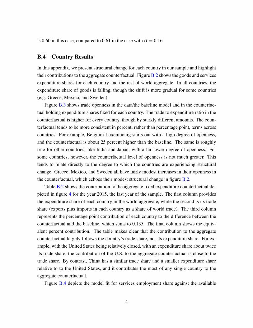
is 0.60 in this case, compared to 0.61 in the case with σ = 0.16.

B.4 Country Results

In this appendix, we present structural change for each country in our sample and highlighttheir contributions to the aggregate counterfactual. Figure B.2 shows the goods and servicesexpenditure shares for each country and the rest of world aggregate. In all countries, theexpenditure share of goods is falling, though the shift is more gradual for some countries(e.g. Greece, Mexico, and Sweden).

Figure B.3 shows trade openness in the data/the baseline model and in the counterfac-tual holding expenditure shares fixed for each country. The trade to expenditure ratio in thecounterfactual is higher for every country, though by starkly different amounts. The coun-terfactual tends to be more consistent in percent, rather than percentage point, terms acrosscountries. For example, Belgium-Luxembourg starts out with a high degree of openness,and the counterfactual is about 25 percent higher than the baseline. The same is roughlytrue for other countries, like India and Japan, with a far lower degree of openness. Forsome countries, however, the counterfactual level of openness is not much greater. Thistends to relate directly to the degree to which the countries are experiencing structuralchange: Greece, Mexico, and Sweden all have fairly modest increases in their openness inthe counterfactual, which echoes their modest structural change in figure B.2.

Table B.2 shows the contribution to the aggregate fixed expenditure counterfactual de-picted in figure 4 for the year 2015, the last year of the sample. The first column providesthe expenditure share of each country in the world aggregate, while the second is its tradeshare (exports plus imports in each country as a share of world trade). The third columnrepresents the percentage point contribution of each country to the difference between thecounterfactual and the baseline, which sums to 0.135. The final column shows the equiv-alent percent contribution. The table makes clear that the contribution to the aggregatecounterfactual largely follows the country’s trade share, not its expenditure share. For ex-ample, with the United States being relatively closed, with an expenditure share about twiceits trade share, the contribution of the U.S. to the aggregate counterfactual is close to thetrade share. By contrast, China has a similar trade share and a smaller expenditure sharerelative to to the United States, and it contributes the most of any single country to theaggregate counterfactual.

Figure B.4 depicts the model fit for services employment share against the available

4

data, the by-country time series analogue to the right panel of figure 3. The average leveland upward trend is well captured for most countries, despite not being an input into thecalibration exercise.

5

Figure B.2: Sectoral expenditure shares by country

1970 1980 1990 2000 20100

0.2

0.4

0.6

0.8

1AUS

1970 1980 1990 2000 20100

0.2

0.4

0.6

0.8

1AUT

1970 1980 1990 2000 20100

0.2

0.4

0.6

0.8

1BLX

1970 1980 1990 2000 20100

0.2

0.4

0.6

0.8

1BRA

1970 1980 1990 2000 20100

0.2

0.4

0.6

0.8

1CAN

1970 1980 1990 2000 20100

0.2

0.4

0.6

0.8

1CHN

1970 1980 1990 2000 20100

0.2

0.4

0.6

0.8

1CYP

1970 1980 1990 2000 20100

0.2

0.4

0.6

0.8

1DEU

1970 1980 1990 2000 20100

0.2

0.4

0.6

0.8

1DNK

1970 1980 1990 2000 20100

0.2

0.4

0.6

0.8

1ESP

1970 1980 1990 2000 20100

0.2

0.4

0.6

0.8

1FIN

1970 1980 1990 2000 20100

0.2

0.4

0.6

0.8

1FRA

1970 1980 1990 2000 20100

0.2

0.4

0.6

0.8

1GBR

1970 1980 1990 2000 20100

0.2

0.4

0.6

0.8

1GRC

1970 1980 1990 2000 20100

0.2

0.4

0.6

0.8

1IDN

1970 1980 1990 2000 20100

0.2

0.4

0.6

0.8

1IND

1970 1980 1990 2000 20100

0.2

0.4

0.6

0.8

1IRL

1970 1980 1990 2000 20100

0.2

0.4

0.6

0.8

1ITA

1970 1980 1990 2000 20100

0.2

0.4

0.6

0.8

1JPN

1970 1980 1990 2000 20100

0.2

0.4

0.6

0.8

1KOR

1970 1980 1990 2000 20100

0.2

0.4

0.6

0.8

1MEX

1970 1980 1990 2000 20100

0.2

0.4

0.6

0.8

1NLD

1970 1980 1990 2000 20100

0.2

0.4

0.6

0.8

1PRT

1970 1980 1990 2000 20100

0.2

0.4

0.6

0.8

1SWE

1970 1980 1990 2000 20100

0.2

0.4

0.6

0.8

1TUR

1970 1980 1990 2000 20100

0.2

0.4

0.6

0.8

1USA

1970 1980 1990 2000 20100

0.2

0.4

0.6

0.8

1ROW

GoodsServices

6

Figure B.3: Trade to expenditure ratio by country

1970 1980 1990 2000 20100

1

2

3AUS

1970 1980 1990 2000 20100

1

2

3AUT

1970 1980 1990 2000 20100

1

2

3BLX

1970 1980 1990 2000 20100

1

2

3BRA

1970 1980 1990 2000 20100

1

2

3CAN

1970 1980 1990 2000 20100

1

2

3CHN

1970 1980 1990 2000 20100

1

2

3CYP

1970 1980 1990 2000 20100

1

2

3DEU

1970 1980 1990 2000 20100

1

2

3DNK

1970 1980 1990 2000 20100

1

2

3ESP

1970 1980 1990 2000 20100

1

2

3FIN

1970 1980 1990 2000 20100

1

2

3FRA

1970 1980 1990 2000 20100

1

2

3GBR

1970 1980 1990 2000 20100

1

2

3GRC

1970 1980 1990 2000 20100

1

2

3IDN

1970 1980 1990 2000 20100

1

2

3IND

1970 1980 1990 2000 20100

1

2

3IRL

1970 1980 1990 2000 20100

1

2

3ITA

1970 1980 1990 2000 20100

1

2

3JPN

1970 1980 1990 2000 20100

1

2

3KOR

1970 1980 1990 2000 20100

1

2

3MEX

1970 1980 1990 2000 20100

1

2

3NLD

1970 1980 1990 2000 20100

1

2

3PRT

1970 1980 1990 2000 20100

1

2

3SWE

1970 1980 1990 2000 20100

1

2

3TUR

1970 1980 1990 2000 20100

1

2

3USA

1970 1980 1990 2000 20100

1

2

3ROW

BaselineFixed Expenditure

7

Table B.2: Contributions to fixed expenditure counterfactual in 2015

Country Expenditure Share Trade Share Ppt. Contribution Pct. ContributionAustralia 1.6% 1.5% 0.002 1.6%Austria 0.5% 1.1% 0.002 1.2%BLX 0.6% 2.3% 0.002 1.8%Brazil 2.2% 1.5% 0.003 2.0%Canada 2.1% 3.0% 0.003 2.5%China 15.0% 12.0% 0.018 13.0%Cyprus 0.0% 0.1% 0.000 0.0%Germany 3.8% 7.9% 0.011 8.4%Denmark 0.3% 0.8% 0.001 0.4%Spain 1.5% 2.0% 0.003 2.6%Finland 0.3% 0.5% 0.001 0.6%France 3.1% 4.1% 0.004 2.9%United Kingdom 3.7% 4.1% 0.005 3.8%Greece 0.3% 0.3% 0.000 0.1%Indonesia 1.2% 0.9% 0.001 1.0%India 2.9% 1.7% 0.002 1.7%Ireland 0.3% 1.2% 0.000 0.2%Italy 2.2% 2.8% 0.005 3.7%Japan 6.3% 4.2% 0.008 5.8%Korea 1.6% 3.5% 0.007 4.8%Mexico 1.5% 2.0% 0.003 2.1%Netherlands 0.8% 2.8% 0.003 2.4%Portugal 0.3% 0.4% 0.001 0.6%Sweden 0.6% 1.1% 0.001 0.9%Turkey 0.9% 1.3% 0.002 1.8%United States 26.3% 11.8% 0.014 10.3%Rest of World 20.1% 25.4% 0.032 23.6%Total 100% 100% 0.135 100%

8

Figure B.4: Services employment share: baseline and data

1970 1980 1990 2000 20100

0.2

0.4

0.6

0.8

1AUS

1970 1980 1990 2000 20100

0.2

0.4

0.6

0.8

1AUT

1970 1980 1990 2000 20100

0.2

0.4

0.6

0.8

1BLX

1970 1980 1990 2000 20100

0.2

0.4

0.6

0.8

1BRA

1970 1980 1990 2000 20100

0.2

0.4

0.6

0.8

1CAN

1970 1980 1990 2000 20100

0.2

0.4

0.6

0.8

1CHN

1970 1980 1990 2000 20100

0.2

0.4

0.6

0.8

1CYP

1970 1980 1990 2000 20100

0.2

0.4

0.6

0.8

1DEU

1970 1980 1990 2000 20100

0.2

0.4

0.6

0.8

1DNK

1970 1980 1990 2000 20100

0.2

0.4

0.6

0.8

1ESP

1970 1980 1990 2000 20100

0.2

0.4

0.6

0.8

1FIN

1970 1980 1990 2000 20100

0.2

0.4

0.6

0.8

1FRA

1970 1980 1990 2000 20100

0.2

0.4

0.6

0.8

1GBR

1970 1980 1990 2000 20100

0.2

0.4

0.6

0.8

1GRC

1970 1980 1990 2000 20100

0.2

0.4

0.6

0.8

1IDN

1970 1980 1990 2000 20100

0.2

0.4

0.6

0.8

1IND

1970 1980 1990 2000 20100

0.2

0.4

0.6

0.8

1IRL

1970 1980 1990 2000 20100

0.2

0.4

0.6

0.8

1ITA

1970 1980 1990 2000 20100

0.2

0.4

0.6

0.8

1JPN

1970 1980 1990 2000 20100

0.2

0.4

0.6

0.8

1KOR

1970 1980 1990 2000 20100

0.2

0.4

0.6

0.8

1MEX

1970 1980 1990 2000 20100

0.2

0.4

0.6

0.8

1NLD

1970 1980 1990 2000 20100

0.2

0.4

0.6

0.8

1PRT

1970 1980 1990 2000 20100

0.2

0.4

0.6

0.8

1SWE

1970 1980 1990 2000 20100

0.2

0.4

0.6

0.8

1TUR

1970 1980 1990 2000 20100

0.2

0.4

0.6

0.8

1USA

1970 1980 1990 2000 20100

0.2

0.4

0.6

0.8

1ROW

BaselineData

9

B.5 Additional Figures

Figure B.5: Deriving sectoral expenditures from sectoral value addedProduction Consumption

ValueAdded

(MultiplybyGO/VAratio)

GrossOutput

(Addimports,subtractexports)

Absorption

Expenditure

(Subtractinputusage)

Gross

Net

Note: Categories in blue represent publicly available data, while categories in blackrepresent imputed moments.

10