Structural Estimation of a Model of School

Choices: the Boston Mechanism vs. Its

Alternatives�

Caterina Calsamigliay, Chao Fuz and Maia Güellx

Feb. 2015 (1st version: May 2014)

Abstract

An important debate centers on what procedure should be used to allocate

students across public schools. We contribute to this debate by developing and

estimating a model of school choices by households under one of the most pop-

ular procedures known as the Boston mechanism (BM). We recover the joint

distribution of household preferences and sophistication types using adminis-

trative data from Barcelona. Our counterfactual policy analyses show that a

change from BM to the Gale-Shapley student deferred acceptance mechanism

would create more losers than winners, while a change from BM to the top

trading cycles mechanism has the opposite e¤ect.

�We thank Yuseob Lee for excellent research assistance. We are grateful to the sta¤ at IDESCAT,and in particular to Miquel Delgado, for their help in processing the data. We thank Steven Durlauf,John Kennan, Chris Taber and workshop participants at UCL, Royal Holloway and Virginia Techfor helpful comments. The authors acknowledge support from a grant from the Institute for NewEconomic Thinking (INET) for the Human Capital and Economic Opportunity Global WorkingGroup (HCEO), an initiative of the Becker Friedman Institute for Research in Economics. The viewsexpressed in this paper are those of the authors and not necessarily those of the funders or personsnamed here. Calsamiglia acknowledges �nancial support by the Spanish Plan Nacional I+D+I(SEJ2005-01481, SEJ2005-01690, SEJ2006-002789-E and FEDER), and the Grupo Consolidado detipo C (ECO2008-04756), the Generalitat de Catalunya (SGR2005-00626), and the Severo Ochoaprogram. Güell acknowledges �nancial support from the Spanish Ministry of Science and Innovation(ECO2011-28965). All errors are ours.

yUniversitat Autonoma de Barcelona and the Barcelona GSEzCorresponding author: Chao Fu, Department of Economics, University of Wisconsin, 1180

Observatory Dr., Madison, WI 53703, USA. Email: cfu@ssc.wisc.edu.xThe University of Edinburgh, CEP(LSE), CEPR, FEDEA, & IZA.

1

1 Introduction

In many countries, every child is guaranteed free access to education in some public

school. However, not all public schools are of the same quality, nor are higher-quality

schools distributed evenly across residential areas. Designed to broaden households�

access to schools beyond their neighborhoods, public school choice systems have been

increasingly adopted in many countries, including the U.S.1 On the one hand, the

quality of schools to which students are assigned can have signi�cant long-term e¤ects

for individual families as well as important implications on the e¢ ciency and equity

for a society.2 On the other hand, schools are endowed with certain capacities and

not all choices can be satis�ed. As a result, how to operationalize school choice, i.e.,

what procedure should be used to assign students to schools, becomes a non-trivial

question that remains heatedly debated on among policy makers and researchers.

One important debate centers around a procedure known as the Boston mechanism

(BM), which was used by Boston Public Schools (BPS) between 1999 and 2005 to

assign K-12 pupils to city schools, and still is one of the most popular school choice

systems in the world. In BM, a household submits its applications in the form of

an ordered list of schools. All applicants are assigned to their �rst choices if there

are enough seats in those schools. If a given school is over-demanded, applicants are

accepted in the order of their priorities for that school.3 Those rejected from their �rst

choices face a dramatically decreased chance of being accepted to any other desirable

schools since they can only opt for the seats that remain free after everyone�s �rst

choice has been considered. As a result, some parents may refrain from ranking schools

truthfully, which makes BM vulnerable to manipulation (Abdulkadiro¼glu and Sönmez

(2003)). In 2005, the BPS replaced BM with the Gale-Shapley student deferred

acceptance mechanism (GS), originally proposed by Gale and Shapley (1962), which

1Some studies have explored exogenous changes in families�school choice sets to study the impactsof school choice on students�achievement, e.g., Abdulkadiro¼glu, Angrist, Dynarsky, Kane and Pathak(2010), Deming, Hastings, Kane and Staiger (2014), Hastings, Kane and Staiger (2009), Lavy (2010),Mehta (2013) and Walter (2013). Other studies focus on how the competition induced by student�sschool choices a¤ects school performance, e.g., Hoxby (2003) and Rothstein (2006).

2See Heckman and Mosso (2014) for a comprehensive review of the literature on human develop-ment and social mobility.

3Priorities for a given school are often determined by whether or not one lives in the zone thatcontains that school, whether or not one has siblings enrolled in the same school, and some othersocioeconomic characteristics, with a random lottery to break the tie.

1

provides incentives for households to reveal their true preferences.4

Although the vulnerability of BM to manipulation is widely agreed upon, it re-

mains unclear whether or not it should be replaced in other cities as well.5 In practice,

the switch decision by the BPS was resisted by some parents.6 In theory, the e¢ ciency

and equity comparison between BM and its alternatives remains controversial.7 The

welfare implications of various mechanisms thus become an empirical question, one

that needs to be answered before a switch from BM to GS or some other mechanisms

is recommended more widely.

To answer this question, one needs to quantify two essential but unobservable

factors underlying households�choices, which is what we do in this paper. The �rst

factor is household preferences, without which one could not compare welfare across

mechanisms even if household choices were observed under each alternative mecha-

nism. Moreover, as choices are often not observed under counterfactual scenarios,

one needs to predict which households would change their behaviors and how their

behaviors would change, were the current mechanism switched to a di¤erent one. The

knowledge of household preferences alone is not enough for this purpose. Although

BM gives incentives for households to act strategically, there may exist non-strategic

households that simply rank schools according to their true preferences.8 A switch

from BM to GS, for example, will induce behavioral changes only among strategic

households who hide their true preferences under BM. Therefore, the knowledge about

the distribution of household types (strategic or non-strategic) becomes a second es-

sential factor for one to assess the impacts of potential reforms in the school choice

system.

We develop a model of school choices under BM by households who di¤er in

both their preferences for schools and their strategic types. Households�preferences

for schools depends on the school quality, the school-home distance and attendance

fees, interacted with household characteristics and a¤ected by household tastes. Non-

4See Abdulkadiro¼glu, Pathak, Roth and Sonmez (2005) for a description of the Boston reform.5Pathak and Sönmez (2013) document switches in Chicago and England from certain forms of the

Boston mechanism to less-manipulable mechanisms, and argue that these switch decisions revealedgovernment preferences against mechanisms that are (excessively) manipulable.

6See Abdulkadiro¼glu, Che, and Yasuda (2011) for examples of the concerns parents had.7See the literature review below.8There is direct evidence that both strategic and non-strategic households exist. For example,

Abdulkadiro¼glu, Pathak, Roth and Sönmez (2006) show that some households in Boston obviouslyfailed to strategize. Calsamiglia and Güell (2014) prove that some households obviously behavestrategically. Estimation results in our paper are such that both types exist.

2

strategic households �ll out their application forms according to their true preferences,

while strategic households take admissions risks into account and may hide their true

preferences.

We apply our model to a rich administrative data set from Barcelona, Spain,

where a BM system has been used to allocate students across the over 300 public

schools. The data contains information on applications, admissions and enrollment

for all Barcelona families who applied for schools in the public school system in the

years 2006 and 2007. In particular, we observe the entire application list submitted

by each applicant, who can rank-list up to 10 out of the over 300 schools. We also

observe applicants�family addresses, hence home-school distances, and other family

characteristics that allow us to better understand their decisions. Between 2006 and

2007, there was a drastic change in the o¢ cial de�nition of school zones that signif-

icantly altered the set of schools a family had priorities for in the school assignment

procedure. We estimate our model via simulated maximum likelihood using the 2006

pre-reform data. We conduct an out-of-sample validation of our estimated model us-

ing the 2007 post-reform data. The estimated model matches the data in both years

well.

The results of the out-of-sample validation provide enough con�dence in the model

to use it to perform counterfactual policy experiments, where we assess the perfor-

mance of two popular and truth-revealing alternatives to BM: GS and the top trad-

ing cycles mechanism (TTC) (Abdulkadiro¼glu and Sönmez (2003)).9 We �nd that

a change from BM to GS bene�ts fewer than 10% of the households while hurting

28% of households. An average household loses by an amount equivalent to a 60-euro

increase in school fees. In contrast, a change from BM to TTC bene�ts over 20%

of households and hurts 19% of them. An average household bene�ts by an amount

equivalent to a 88-euro decrease in school fees. Compared to TTC, BM and GS inef-

�ciently assign households to closer-by but lower-quality schools. On the equity side,

a switch from BM to GS is more likely to bene�t those who live in higher-school-

quality zones than those who live in lower-school-quality zones, hence enlarging the

cross-zone inequality. In contrast, the quality of the school zone a household lives in

does not impact its chance to win or to lose in a switch from BM to TTC. We also

�nd that while TTC enables 76% of households whose favorite schools are out of their9TTC was inspired by top trading cycles introduced by Shapley and Scarf (1974) and adapted by

Abdulkadiro¼glu and Sönmez (2003). To our knowledge, only New Orleans has implemented TTC.

3

zones to attend their favorite schools, this fraction is only 59% under BM and 52%

under GS.

Our paper contributes to the literature on school choices, in particular, the liter-

ature on the design of centralized choice systems initiated by Balinski and Sönmez

(1999) for college admissions, and Abdulkadiro¼glu and Sönmez (2003) for public school

choice procedures.10 Abdulkadiro¼glu and Sönmez (2003) formulate the school choice

problem as a mechanism design problem, and point out the �aws of BM, including

manipulability. They also investigate the theoretical properties of two alternatives

of BM: GS and TTC. Since then, researchers have been debating on the properties

of BM. Some studies suggest that the fact that strategic ranking may be bene�cial

under BM creates a potential issue of equity since parents who act honestly (non-

strategic parents) may be disadvantaged by those who are strategically sophisticated

(e.g., Pathak and Sönmez (2008)). Using the pre-2005 data provided by the BPS,

Abdulkadiro¼glu, Pathak, Roth and Sönmez (2006) �nd that households that obvi-

ously failed to strategize were disproportionally unassigned. Calsamiglia and Miralles

(2014) show that under certain conditions, the only equilibrium under BM is the one

in which families apply for and are assigned to schools in their own school zones,

which causes concerns about inequality across zones. Besides equity, BM has also

been criticized on the basis of e¢ ciency. Experimental evidence from Chen and Sön-

mez (2006) and theoretical results from Ergin and Sönmez (2006) show that GS is

more e¢ cient than BM in complete information environments. However, in a recent

series of studies, Abdulkadiro¼glu, Che, and Yasuda (2011); Featherstone and Niederle

(2011); and Miralles (2008) all provide examples of speci�c environments where BM

is more e¢ cient than GS. Abdulkadiro¼glu, Che, and Yasuda (2011) also point out

that somenon-strategic parents may actually be better o¤ under BM than under GS.

Although there have been extensive theoretical discussions about the strength

and weakness of alternative school choice mechanisms, empirical studies designed to

quantify the di¤erences between these alternatives have been sparse.11 Hwang (2014)

set identi�es household preferences under the assumption that a household would

rank a popular school on its report only if it prefers this school to less popular ones.

10While student priorities for a certain college depends on the college�s own "preferences" overstudents; student priorities for public schools are de�ned by the central administration.11With a di¤erent focus, Abdulkadiro¼glu, Agarwal and Pathak (2014) show the bene�ts of cen-

tralizing school choice procedures, using data from New York city where high school choices used tobe decentralized.

4

He (2012) estimates an equilibrium model of school choice under BM using data

from one neighborhood in Beijing that contains four schools, for which households

have equal priorities to attend. Under certain assumptions, he estimates household

preference parameters by grouping household choices, without having to model the

distribution of household sophistication types. On the one hand, the approach in

He (2012) allows one to be agnostic about the distribution of household strategic

types during the estimation, hence imposing fewer presumptions on the data. On

the other, it restricts his model�s ability to conduct cross-mechanism comparisons.

Our paper complements He (2012) by estimating both households�preferences and

the distribution of their strategic types. We apply our model to the administrative

data that contain the application and assignment outcomes for the entire city of

Barcelona, where households are given priorities to schools in their own school zones.

With access to this richer data set, we are able to form a more comprehensive view of

the alternative mechanisms in terms of the overall household welfare and the cross-

neighborhood inequality.

Under the assumption that all households behave strategically, Agarwal and So-

maini (2014) interpret a household�s submitted report as a choice of a probability

distribution over assignments. In a two-step estimation procedure, they estimate �rst

the assignment probabilities and then preferences using a Gibbs�sampler. They apply

their method to the Controlled Choice Plan (CPS) in Cambridge, MA, in which each

student can rank up to 3 out of 25 possible programs. Similar to our results, they

also �nd that the average student welfare would be lower under the counterfactual

GS compared to the current system. Agarwal and Somaini (2014) and our paper

complement each other well. Both papers exploit the observed assignment outcomes

in a large market and estimate household preferences under manipulable mechanisms

without having to solve for the equilibrium. Given the assumption that all households

are strategic, their method allows one to avoid the computational burden of solving

for the optimal report given a simulated draw of the utility during the estimation. We

use a di¤erent method that allows us to estimate both household preferences and the

distribution of strategic types. Assuming an intuitive two-step boundedly-rational

decision process among sophisticated households, we show how one can feasibly solve

and estimate a model where households face an otherwise unmanageably large number

of choices.

Also related to our paper are studies that use out-of-sample �ts to validate the

5

estimated model.12 Some studies do so by exploiting random social experiments,

e.g., Wise (1985), Lise, Seitz and Smith (2005) and Todd and Wolpin (2006), or

lab experiments, e.g., Bajari and Hortacsu (2005). Other studies do so using major

regime shifts. McFadden and Talvitie (1977), for example, estimate a model of travel

demand before the introduction of the BART system, forecast the level of patronage

and then compare the forecast to actual usage after BART�s introduction. Pathak

and Shi (2014) aim at conducting a similar validation exercise on the data of school

choices before and after a major change in households�choice sets of public schools,

introduced in Boston in 2013.13 Some studies, including our paper, deliberately hold

out data to use for validation purposes. Lumsdaine, Stock and Wise (1992) estimate

a model of worker retirement behavior of workers using data before the introduction

of a temporary one-year pension window and compare the forecast of the impact

of the pension window to the actual impact. Keane and Mo¢ tt (1998) estimate

a model of labor supply and welfare program participation using data after federal

legislation that changed the program rules. They used the model to predict behavior

prior to that policy change. Keane and Wolpin (2007) estimate a model of welfare

participation, schooling, labor supply, marriage and fertility on a sample of women

from �ve US states and validate the model based on a forecast of those behaviors on

a sixth state.

The rest of the paper is organized as follows. The next section gives some back-

ground information about the public school system in Barcelona. Section 3 describes

the model. Section 4 explains our estimation and identi�cation strategy. Section 5

describes the data. Section 6 presents the estimation results. Section 7 conducts coun-

terfactual experiments. The last section concludes. The appendix contains further

details and additional tables.12See Keane, Todd and Wolpin (2011) for a comprehensive review.13The authors are waiting for the post-reform data to �nish their project.

6

2 Background

2.1 The Public School System in Spain

The public school system in Spain consists of over 300 schools that are of two types:

public and semi-public.14 Public schools are fully �nanced by the autonomous com-

munity government and are free to attend.15 The operation of public schools follows

rules that are de�ned both at the national and at the autonomous community level.

Depending on the administrative level at which it is de�ned, a rule applies uniformly

to all public schools nationally or autonomous-community-wise. This implies that all

public schools in the same autonomous community are largely homogenous in terms

of the assignment of teachers, school infrastructure, class size, curricula, and the level

of (full) �nancial support per pupil.

Semi-public schools are run privately and funded via both public and private

sources.16 The level of public support per pupil for semi-public schools is de�ned

at the autonomous community level, which is about 60% of that for public schools.

Semi-public schools are allowed to charge enrollee families for complementary ser-

vices. In Barcelona, the service fee per year charged by semi-public schools is 1; 280

euros on average with a standard deviation of 570 euros.17 On average, of the total

�nancial resources for semi-public schools, government funding accounts for 63%, ser-

vice fees account for 34%, and private funding accounts for 3%. Semi-public schools

have much higher level of autonomy than public schools. They can freely choose

their infrastructure facilities, pedagogical preferences and procedures. Subject to the

government-imposed teacher credential requirement, semi-public schools have controls

over teacher recruiting and dismissal. However, there are some important regulations

semi-public schools are subject to. In particular, all schools in the public school sys-

tem, public or semi-public, have to unconditionally accept all the students that are

14Semi-public schools were added into the system under a 1990 national educational reform inSpain (LOGSE). In our sample period, there were 158 public schools and 159 semi-public schools.15Spain is divided into 17 autonomous communities, which are further divided into provinces

and municipalities. A large fraction of educational policies are run at the autonomous community(Comunidades Autonomas) and municipality levels (municipios) following policies determined bothat the national and at the local levels. In particular, the Organic Laws (Leyes Orgánicas) establishbasic rules to be applied nationally; while autonomous communities further develop these rulesthrough what are called Decretos.16See http://www.idescat.cat/cat/idescat/publicacions/cataleg/pdfdocs/dossier13.pdf for details.17The median annual housesehold income is 25; 094 euros in Spain and 26; 418 euros in Catalunya.

7

assigned to them via the centralized school choice procedure that we describe in the

next subsection; and no student can be admitted to the public school system with-

out going through the centralized procedure. In addition, all schools have the same

national limit on class sizes.

Outside of the public school system, there are a small number of private schools,

accounting for only 4% of all schools in Barcelona. Private schools receive no public

funding and charge very high tuition, ranging from 5,000 to 16,000 euros per year

in Barcelona. Private schools are subject to very few restrictions on their operation;

and they do not participate in the centralized school choice program.18

2.2 School Choice within the Public School System

The Organic Law 8/1985 establishes the right for families to choose schools in the

public school system for their children. The national reform in 1990 (LOGSE) ex-

tended families�right to guarantee the universal access for a child 3 years or older to

a seat in the public school system, by requiring that preschool education (ages 3-5)

be o¤ered in the same facilities that o¤er primary education (ages 6-12). Although

a child is guaranteed a seat in the public school system, individual schools can be

over-demanded. The Organic Law from 2006 (LOE) speci�es broad criteria that au-

tonomous communities shall use to resolve the overdemand for schools. Catalunya,

the autonomous community for the city of Barcelona, has its own Decretos in which

it speci�es, under the guideline of LOE, how overdemand for given schools shall be

resolved. In particular, it describes broad categories over which applicants may be

ranked and prioritized, known as the priority rules.

Families get access to schools in the public school system via a centralized school

choice procedure run at the city or municipality level, in which almost all families

participate.19 Every April, participating families with a child who turns three in that

calendar year are asked to submit a ranked list of up to 10 schools. Households who

submit their applications after the deadline (typically between April 10th and April

20th) can only be considered after all on-time applicants have been assigned.20 All

18For this reason, information on private schools is very limited. Given the lack of information onprivate schools and the small fraction of schools they account for, we treat private schools as partof the (exogenous) outside option in the model.19For example, in 2007, over 95% of families with a 3-year old child in Barcelona participated in

the application procedure.20See Calsamiglia and Güell (2014) for more details on the application forms and the laws under-

8

applications are typed into a centralized system, which assigns students to schools via

a Boston mechanism.21 The �nal assignment is made public and �nalized between

April and May, and enrollment happens at the beginning of September, when school

starts. In the assignment procedure, all applicants are assigned to their �rst choice

if there are enough seats. If there is overdemand for a school, applicants are priori-

tized according to the government-speci�ed priority rules. In Catalunya, a student�s

priority score is a sum of various priority points: the presence of a sibling in the

same school (40 points), living in the zone that contains that school (30 points), and

some other characteristics of the family or the child (e.g., disability (10 points)). Ties

in total priority scores are broken through a fair lottery. The assignment in every

round of the procedure is �nal, which implies that an applicant rejected from her

�rst-ranked school can get into her second-ranked school only if this school still has

a free seat after the �rst round. The same rule holds for all later rounds.

In principle, a family can change schools within the public school system after

the assignment. This is feasible only if the receiving school has a free seat, which is

a near-zero-probability event in popular schools. The same di¢ culty of transferring

schools persists onto the preschool-to-primary-school transition because a student has

the priority to continue her primary-school education in the same school she enrolled

for preschool education, and because school capacities remain the same in preschools

and primary schools (which are o¤ered in the same facilities). A family�s initial school

choice continues to a¤ect the path into secondary schools as students are given prior-

ities to attend speci�c secondary schools depending on the schools they enrolled for

primary-school education. On the one hand, besides the direct e¤ect of quality of the

preschool on their children�s development, families�school choice for their 3-year-old

children have long-term e¤ects on their children�s educational path due to institu-

tional constraints. On the other hand, the highly centralized management of public

schools in Barcelona reduces the stakes families take by narrowing the di¤erences

across schools.

lying this procedure.21We will describe the exact procedure in the model section.

9

2.3 Changes in the De�nition of Zones (2007)

Before 2007, the city of Barcelona was divided into �xed zones; families living in

a given zone had priorities for all the schools in that zone.22 Depending on their

speci�c locations within a zone, families could have priorities for in-zone schools that

were far away from their residence while no priority for schools that were close-by but

belonged to a di¤erent zone. This is particularly true for families living around the

corner of di¤erent zones. In 2007, a family�s school zone is rede�ned as the smallest

area around its residence that covered the closest 3 public and the closest 3 semi-

public schools, for which the family was given residence-based priorities.23 The 2007

reform was announced abruptly on March 27th, 2007, before which there had been

no public discussions about it. Families were informed via mail by March 30th, who

had to submit their lists by April 20th.

3 Model

3.1 Primitives

There are J public schools distributed across various school zones in the city. In the

following, schools refer to non-private (public, semi-public) schools unless speci�ed

otherwise. There is a continuum of households/applicants/parents of measure 1 (we

use the words household, applicant and parent interchangeably). Each household

submits an ordered list of schools before the o¢ cial deadline, after which a centralized

procedure is used to assign students according to their applications, the available

capacity of each school and a priority structure.24 A student can either choose to

attend the school she is assigned to or opt for the outside option.

22Before 2007, zones were de�ned di¤erently for public and semi-public schools. A family livingat a given location had priorities for a set of public schools de�ned by its public-school zone, anda set of semi-public schools de�ned by its semi-public-school zone. Throughout the paper, in-zoneschools refer to the union of these two sets of schools; and two families are said to live in the samezone if they have the same set of in-zone schools.23There were over 5,300 zones under this new de�nition. See Calsamiglia and Güell (2014) for a

detailed description of the 2007 reform.24As mentioned in the background section, almost all families participate in the application proce-

dure. For this reason, we assume that the cost of application is zero and that all families participate.This is in contrast with the case of college application, which can involve signi�cant monetary andnon-monetary application costs, e.g., Fu (2014).

10

3.1.1 Schools

Each school j is endowed with a location lj and a vector wj of characteristics consisting

of school quality, capacity, tuition and an indicator of semi-public school. School

characteristics are public information.25 A school�s capacity lie between (0; 1) hence

no school can accommodate all students. The total capacity of all schools is at least

1, hence each student is guaranteed a seat in the public school system.

3.1.2 Households

A household i is endowed with characteristics xi; a home location li, tastes �i = f�ijgjfor schools j = 1; ::; J; and a type T 2 f0; 1g (non-strategic or strategic):26 Householdtastes and types, known to households themselves, are unobservable to the researcher.

The fraction of strategic households varies with household characteristics and home

locations, given by � (xi; li) : Types di¤er only in their behaviors, which will become

clear when we specify a household�s problem, but all households share the same

preference parameters.

As is common in discrete choice models, the absolute level of utility is not identi-

�ed, we normalize the ex-ante value of the outside option to zero for all households.

That is, a household�s evaluation of each school is relative to its evaluation of the

outside option, which may di¤er across households. Let dij = d (li; lj) be the distance

between household i and school j, and di = fdijgj be the vector of distances to allschools for i: Household i�s utility from attending school j; regardless of its type, is

given by

uij = U (wj; xi; dij) + �ij:

where U (wj; xi; dij) is a function of the school and household characteristics and

home-school distance, and �ij is i0s idiosyncratic tastes for school j:27 We assume the

25We assume that households have full information about school characteristics. Our data do notallow us to separate preferences from information frictions. Some studies have taken a natural or�eld experiment approach to shed lights on how information a¤ects schooling choices, e.g., Hastingsand Weinstein (2008) and Jensen (2010).26Our model is �exible enough to accomodate but does not impose any restriction on the existence

of either strategic and non-strategic types. The distribution of the two types is an empirical question.With a parsimonious two-point distribution of sophistication types, the model �ts the data well. Weleave, as a future extension, more general speci�cations of the type distribution with more than twolevels of sophistication.27Our initial estimation allows a function of zone characteristics to also enter household utility

function in order to capture some common preference factors that exist among households living in

11

vector �i s i:i:d:F� (�) :28

Between application and enrollment (about 6 months), the value of the outside

option is subject to a shock �i s i:i:d:N(0; �2�). A parent knows the distribution of

�i�s before submitting the application, and observes it afterwards. For example, a

parent may experience a wage shock that changes her ability to pay for the private

school. This post-application shock rationalizes the fact that some households in the

data chose the outside option even after being assigned to the schools of their �rst

choice.

3.2 Priority and Assignment

In this subsection, we describe the o¢ cial rules on priority scores and the assignment

procedure.

3.2.1 The Priority Structure

A household i is given a priority score sij for each of the schools j = 1; :::; J; deter-

mined by household characteristics, its home location and the location of the school.

Locations matter only up to whether or not the household locates within the school

zone a school belongs to. Let zl be the school zone that contains location l. House-

hold characteristics xi consists of two parts: demographics x0i and the vector of length

J fsibijgj ; where sibij = 1 (sibij = 0) if student i has some (no) sibling enrolled inschool j. Priority score sij is given by

sij = x0i a+ b1I

�li 2 zlj

�+ b2sibij; (1)

where a is the vector of o¢ cial bonus points that applies to household demographics,

b1 > 0 is the bonus point for schools within one�s zone, I�li 2 zlj

�indicates whether

or not household i lives in school j�s zone, and b2 is the bonus point for the school one�s

the same zone. In a likelihood ratio test, we cannot reject that the simpler speci�cation presentedhere explains the data just as well as the more complicated version. As most studies on the schoolchoice mechanisms, we abstract from peer e¤ects and social interactions from our model. The majorcomplication is the potential multiple equilibria problem embedded in the presence peer e¤ects andsocial interactions, which implies that truth-telling may no longer hold even under mechanisms suchas GS and TTC. See Epple and Romano (2011) and Blume, Brock, Durlauf and Ioannides (2011)for comprehensive reviews on peer e¤ects in education and on social interactions, respectively.28In particular, we assume �ij s i:i:d:N(0; �2� ).

12

sibling is enrolled in.29 To reduce its own computational burden, the administration

stipulates that a student�s priority score of her �rst choice carries over for all schools

on her application list.30

3.2.2 The Assignment Procedure: BM

Schools are gradually �lled up over rounds. There are R < J rounds, where R is also

the o¢ cial limit on the length of an application list.

Round 1: Only the �rst choices of the students are considered. For each school,

consider the students who have listed it as their �rst choice and assign seats of the

school to these students one at a time following their priority scores from high to low

(with random lotteries as tie-breakers) until either there are no seats left or there is

no student left who has listed it as her �rst choice.

Round r 2 f2; 3; :::; Rg: Only the rth choices of the students not previously as-signed are considered. For each school with still available seats, assign the remaining

seats to these students one at a time following their priority scores from high to low

(with random lotteries as tie-breakers) until either there are no seats left or there is

no student left who has listed it as her rth choice.

The procedure terminates after any step r � R when every student is assigned aseat at a school, or if the only students who remain unassigned listed no more than r

choices. Let prj (sij) be the probability of being admitted to school j in Round r for

a student with priority score sij for school j, who listed j as the rth application. The

assignment procedure implies that the admissions probability is (weakly) decreasing

in priority scores within each round, and is (weakly) decreasing over rounds for all

priority scores. A student who remains unassigned after the procedure ends can

propose a school that still has empty seat and be assigned to it.

3.3 Household Problem

We start with a household�s enrollment problem. After seeing the post-application

shock �i to its outside option and the assignment result, a household chooses the

29It follows from the formula that a student can have 2; 3 or 4 levels of priority scores, dependingon whether or not the school is in-zone or out-of-zone, whether or not one has sibling(s) in somein-zone and/or out-of-zone schools. See the appendix for details.30For example, if a student lists an in-zone (out-of-zone) sibling school as her �rst choice, she

carries x0i a+ b1 + b2 (x0i a+ b2) for all the other schools she listed regardless of whether or not they

are within her zone and whether or not she has a sibling in those schools.

13

better between the school it is assigned to and the outside option. Let the expected

value of being assigned to school j be vij; such that

vij = E�i max fuij; �ig :

As seen from the assignment procedure, if rejected by all schools on its list, a house-

hold can opt for a school that it prefers the most within the set of schools that still

have empty seats after everyone�s applications have been considered. Label these

schools as "leftovers," and i�s favorite "leftover" school as i�s backup. The value (vi0)

of being assigned to its backup school for household i is given by

vi0 = max fvijgj2leftovers :

In the following, we describe a household�s application problem, in which it chooses

an ordered list of up toR schools. We do this separately for non-strategic and strategic

households.

3.3.1 Non-Strategic Households

A non-strategic household lists schools on its application form according to its true

preferences fvijgj : Without further assumptions, any list of length n (1 � n � R)that consists of the ordered top n schools according to fvijgj is consistent with non-strategic behavior. We impose the following extra structure: suppose household i

ranks its backup school as its n�i -th favorite, then the length of i�s application list niis such that

ni � min fn�i ; Rg : (2)

That is, when there are still slots left on its application form, a non-strategic household

will list at least up to its backup school.

Let A0i =�a01; a

02; ::a

0ni

be an application list for non-strategic (T = 0) household

i, where a0r is the ID of the rth-listed school and ni satis�es (2) : The elements in A0i

are given by

a01 = argmax fvijgj (3)

a0r = argmax fvijjj 6= ar0<rgj ; for 1 < r � min fn�i ; nig :

14

De�ne A0 (xi; �i; li) as the set of lists that satisfy (2) and (3) for a non-strategic

household with characteristics xi; location li and tastes �i. If n�i � R; the set A0 (�)is a singleton, and the length of the application list ni = R: If n�i < R, all lists in

the set A0 (�) are identical up to the �rst n�i elements, and they all imply the sameallocation outcome for household i.

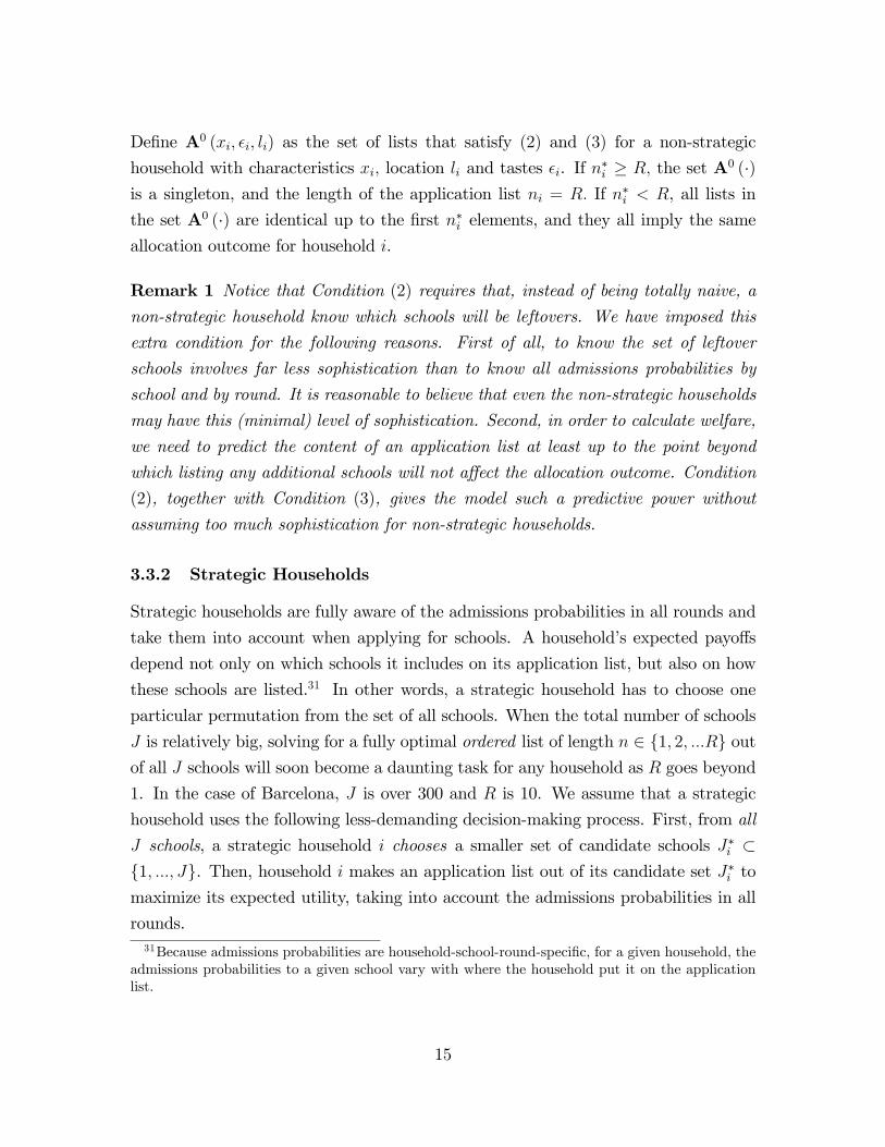
Remark 1 Notice that Condition (2) requires that, instead of being totally naive, anon-strategic household know which schools will be leftovers. We have imposed this

extra condition for the following reasons. First of all, to know the set of leftover

schools involves far less sophistication than to know all admissions probabilities by

school and by round. It is reasonable to believe that even the non-strategic households

may have this (minimal) level of sophistication. Second, in order to calculate welfare,

we need to predict the content of an application list at least up to the point beyond

which listing any additional schools will not a¤ect the allocation outcome. Condition

(2), together with Condition (3), gives the model such a predictive power without

assuming too much sophistication for non-strategic households.

3.3.2 Strategic Households

Strategic households are fully aware of the admissions probabilities in all rounds and

take them into account when applying for schools. A household�s expected payo¤s

depend not only on which schools it includes on its application list, but also on how

these schools are listed.31 In other words, a strategic household has to choose one

particular permutation from the set of all schools. When the total number of schools

J is relatively big, solving for a fully optimal ordered list of length n 2 f1; 2; :::Rg outof all J schools will soon become a daunting task for any household as R goes beyond

1. In the case of Barcelona, J is over 300 and R is 10. We assume that a strategic

household uses the following less-demanding decision-making process. First, from all

J schools, a strategic household i chooses a smaller set of candidate schools J�i �f1; :::; Jg. Then, household i makes an application list out of its candidate set J�i tomaximize its expected utility, taking into account the admissions probabilities in all

rounds.31Because admissions probabilities are household-school-round-speci�c, for a given household, the

admissions probabilities to a given school vary with where the household put it on the applicationlist.

15

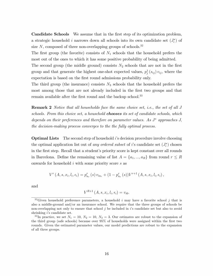
Candidate Schools We assume that in the �rst step of its optimization problem,

a strategic household i narrows down all schools into its own candidate set (J�i ) of

size N , composed of three non-overlapping groups of schools.32

The �rst group (the favorite) consists of N1 schools that the household prefers the

most out of the ones to which it has some positive probability of being admitted.

The second group (the middle ground) consists N2 schools that are not in the �rst

group and that generate the highest one-shot expected values, p1j (sij) vij; where the

expectation is based on the �rst round admissions probability only.

The third group (the insurance) consists N3 schools that the household prefers the

most among those that are not already included in the �rst two groups and that

remain available after the �rst round and the backup school.33

Remark 2 Notice that all households face the same choice set, i.e., the set of all Jschools. From this choice set, a household chooses its set of candidate schools, whichdepends on their preferences and therefore on parameter values. As J� approaches J;

the decision-making process converges to the the fully optimal process.

Optimal Lists The second step of household i�s decision procedure involve choosing

the optimal application list out of any ordered subset of i�s candidate set (J�i ) chosen

in the �rst step. Recall that a student�s priority score is kept constant over all rounds

in Barcelona. De�ne the remaining value of list A = fa1; :::; aRg from round r � Ronwards for household i with some priority score s as

V r (A; s; xi; li; �i) = prar (s) viar + (1� p

rar (s))V

r+1 (A; s; xi; li; �i) ,

and

V R+1 (A; s; xi; li; �i) = vi0:

32Given household preference parameters, a household i may have a favorite school j that isalso a middle-ground and/or an insurance school. We require that the three groups of schools benon-overlapping not only to ensure that school j be included in i�s candidate set but also to avoidshrinking i�s candidate set.33In practice, we set N1 = 10; N2 = 10; N3 = 3: Our estimates are robust to the expansion of

the third group (safe schools) because over 95% of households were assigned within the �rst tworounds. Given the estimated parameter values, our model predictions are robust to the expansionof all three groups.

16

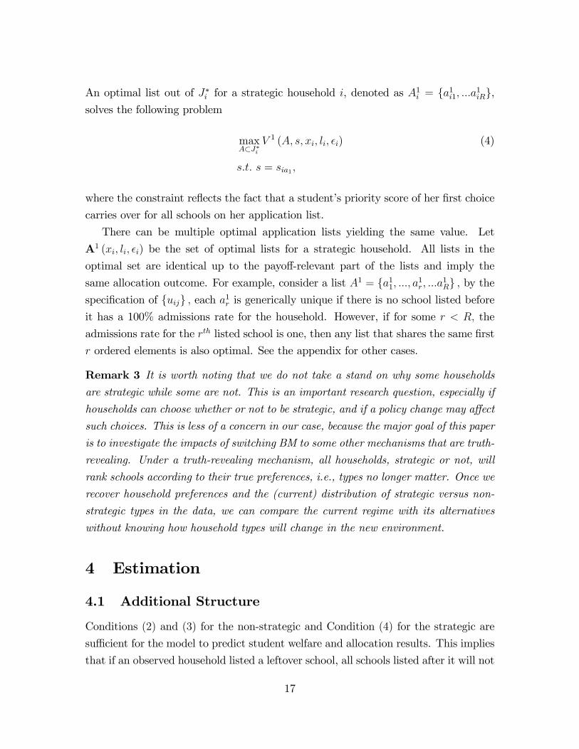
An optimal list out of J�i for a strategic household i, denoted as A1i = fa1i1; :::a1iRg,

solves the following problem

maxA�J�i

V 1 (A; s; xi; li; �i) (4)

s:t: s = sia1 ;

where the constraint re�ects the fact that a student�s priority score of her �rst choice

carries over for all schools on her application list.

There can be multiple optimal application lists yielding the same value. Let

A1 (xi; li; �i) be the set of optimal lists for a strategic household. All lists in the

optimal set are identical up to the payo¤-relevant part of the lists and imply the

same allocation outcome. For example, consider a list A1 = fa11; :::; a1r; :::a1Rg ; by thespeci�cation of fuijg ; each a1r is generically unique if there is no school listed beforeit has a 100% admissions rate for the household. However, if for some r < R; the

admissions rate for the rth listed school is one, then any list that shares the same �rst

r ordered elements is also optimal. See the appendix for other cases.

Remark 3 It is worth noting that we do not take a stand on why some householdsare strategic while some are not. This is an important research question, especially if

households can choose whether or not to be strategic, and if a policy change may a¤ect

such choices. This is less of a concern in our case, because the major goal of this paper

is to investigate the impacts of switching BM to some other mechanisms that are truth-

revealing. Under a truth-revealing mechanism, all households, strategic or not, will

rank schools according to their true preferences, i.e., types no longer matter. Once we

recover household preferences and the (current) distribution of strategic versus non-

strategic types in the data, we can compare the current regime with its alternatives

without knowing how household types will change in the new environment.

4 Estimation

4.1 Additional Structure

Conditions (2) and (3) for the non-strategic and Condition (4) for the strategic are

su¢ cient for the model to predict student welfare and allocation results. This implies

that if an observed household listed a leftover school, all schools listed after it will not

17

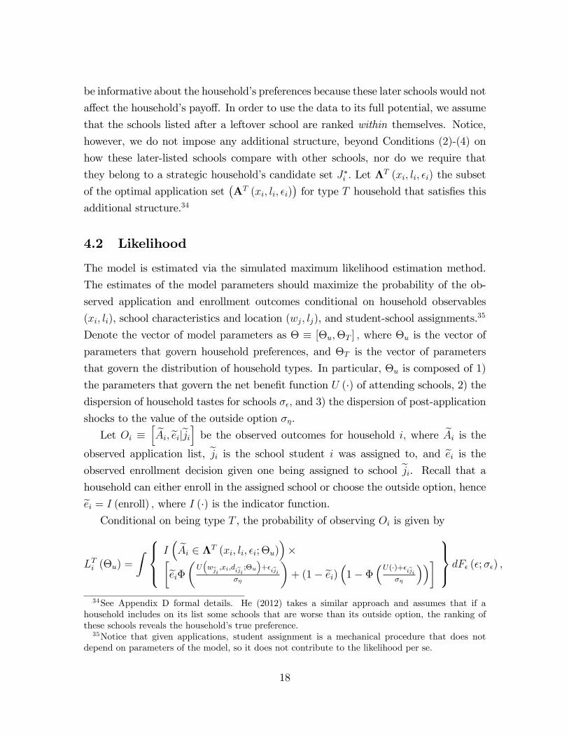
be informative about the household�s preferences because these later schools would not

a¤ect the household�s payo¤. In order to use the data to its full potential, we assume

that the schools listed after a leftover school are ranked within themselves. Notice,

however, we do not impose any additional structure, beyond Conditions (2)-(4) on

how these later-listed schools compare with other schools, nor do we require that

they belong to a strategic household�s candidate set J�i : Let �T (xi; li; �i) the subset

of the optimal application set�AT (xi; li; �i)

�for type T household that satis�es this

additional structure.34

4.2 Likelihood

The model is estimated via the simulated maximum likelihood estimation method.

The estimates of the model parameters should maximize the probability of the ob-

served application and enrollment outcomes conditional on household observables

(xi; li), school characteristics and location (wj; lj), and student-school assignments.35

Denote the vector of model parameters as � � [�u;�T ] ; where �u is the vector of

parameters that govern household preferences, and �T is the vector of parameters

that govern the distribution of household types. In particular, �u is composed of 1)

the parameters that govern the net bene�t function U (�) of attending schools, 2) thedispersion of household tastes for schools ��; and 3) the dispersion of post-application

shocks to the value of the outside option ��.

Let Oi �h eAi; eeijejii be the observed outcomes for household i; where eAi is the

observed application list, eji is the school student i was assigned to, and eei is theobserved enrollment decision given one being assigned to school eji. Recall that ahousehold can either enroll in the assigned school or choose the outside option, henceeei = I (enroll) ; where I (�) is the indicator function.Conditional on being type T , the probability of observing Oi is given by

LTi (�u) =

Z 8><>:I� eAi 2 �T (xi; li; �i; �u)���eei��U

�weji ;xi;dieji ;�u

�+�ieji

��

�+ (1� eei)�1� ��U(�)+�ieji��

���9>=>; dF� (�;��) ;

34See Appendix D formal details. He (2012) takes a similar approach and assumes that if ahousehold includes on its list some schools that are worse than its outside option, the ranking ofthese schools reveals the household�s true preference.35Notice that given applications, student assignment is a mechanical procedure that does not

depend on parameters of the model, so it does not contribute to the likelihood per se.

18

where �T (xi; li; �i; �u) is the subset of model-predicted optimal application lists for a

type-T household with (xi; li; �i) as described in the previous subsection. ��U(�)+�ieji

��

�is the model-predicted probability that this household will enroll in school eji; whichhappens if only if the post-application shock to the outside option is lower than the

utility of attending eji.To obtain household i�s contribution to the likelihood, we integrate over the type

distribution

Li (�) = �(xi; li; �T )L1i (�u) + (1� �(xi; li; �T ))L0i (�u) :

Finally, the total log likelihood of the whole sample is given by

$ (�) =Xi

ln (Li (�)) :

4.3 Identi�cation

We give an overview of the identi�cation in this subsection and leave the formal proof

in Appendix B2. Besides the regular conditions such as utility functions be continu-

ous, the identi�cation relies on the following assumptions.

IA1: There does not exist a vector of household observable x and a school j; such

that all households with x has zero admissions probabilities to school j.

IA2: Household tastes � are drawn from an i.i.d. unimodal distribution, with mean

normalized to zero. Tastes are independent of school observables w, household ob-

servables (x; l) and household type (T ) :

IA3: At least one continuous variable in the utility function is excluded from the type

distribution. Conditional on variables that enter the type distribution function, the

excluded variable is independent of household type T:

To illustrate the identi�cation challenge, consider a situation where each household

only applies to one school, which is a less favorable situation for identi�cation because

we would have less information, and suppose there is no post-application shock.36 If

all households are non-strategic, the model boils down to a multinomial discrete choice

model with a household choosing the highest U (wj; xi)+�ij. The identi�cation of such

models is well-established under very general conditions (e.g., Matzkin (1993)). If all

36The post-application shock is identi�ed from the observed allocation and enrollment outcomes.

19

households are strategic, the model is modi�ed only in that a household considers

the admissions probabilities fpijgj and chooses the option with the highest expectedvalue. With fpijg observed from the data, this model is identi�ed with the additionalcondition IA1, which requires that for any x; the expected value of applying for school

j is not degenerate: The challenge exists because we allow for a mixture of both types

of households. In the following, we �rst explain IA2-IA3, then give the intuition

underlying the identi�cation proof.

We observe application lists with di¤erent distance-quality-risk combinations with

di¤erent frequencies in the data. The model predicts that households of the same type

tend to make similar application lists. Given IA2, the distributions of type-related

variables will di¤er around the modes of the observed choices, which informs us of

the correlation between type T and these variables. IA3 guarantees that di¤erent

behaviors can arise from exogenous variations within a type. To satisfy IA3, we need

to make some restrictions on how household observables (xi; li) enter type distribution

and utility. Conditional on distance, a non-strategic household may not care too

much about living to the left or the right of a school, but a strategic household may

be more likely to have chosen a particular side so as to take advantage of the priority

zone structure.37 However, given that households, strategic or not, share the same

preferences about school characteristics and distances, there is no particular reason

to believe that everything else being equal, the strategic type will live closer to a

particular school than the non-strategic type do only for the sake of being close. In

other words, because the only di¤erence between a strategic type and a non-strategic

type is whether or not one considers the admissions probabilities, which are a¤ected

by one�s home location only via the zone to which it belongs to, we assume that home

location li enters the type distribution only via the school zone zli, i.e.,

� (xi; li) = � (xi; zli) :

In contrast, household utility depends directly on the home-school distance vector di;

where dij = d (li; lj). Conditional on being in the same school zone, households with

similar characteristics x but di¤erent home addresses still face di¤erent home-school

distance vectors d, as required in IA3.

37Without directly modeling households�location choices, we allow household types to be corre-lated with the characteristics of the school zones they live in. We leave the incorporation of householdlocation choices for future extensions.

20

Conditional on (x; zl) ; the variation in d induces di¤erent behaviors within the

same type; and conditional on (x; zl; d) ; di¤erent types behave di¤erently. In par-

ticular, although households share the same preference parameters, di¤erent types of

households will behave as if they have di¤erent sensitivities to distance. For example,

consider households with the same (x; zl) and a good school j out of their zone zl, as

the distance to j decreases along household addresses, more and more non-strategic

households will apply to j because of the decreasing distance cost. However, the re-

actions will be much less obvious among the strategic households, because they take

into account the risk of being rejected, which remains unchanged no matter how close

j is as long as it is out of zl. In fact, as the home address moves closer and closer to the

border of the school zones, strategic households may appear to "prefer" schools that

are further away. The di¤erent distance-elasticity among households therefore inform

us of the type distribution within (x; zl).38 This identi�cation argument does not

depend on speci�c parametric assumptions. For example, Lewbel (2000) shows that

similar models are semiparametrically identi�ed when an IA3-like excluded variable

with a large support exists. However, to make the exercise feasible, we have assumed

speci�c functional forms. Appendix B2 shows a formal proof of identi�cation given

these additional speci�cations.

The identi�cation of our model is further facilitated by the fact that we can

partly observe household type directly from the data: there is one particular type of

"mistakes" that a strategic household will never make, which is a su¢ cient (but not

necessary) condition to spot a non-strategic household. Intuitively, if a household�s

admissions status is still uncertain for all schools listed so far, and there is another

school j it desires, it never pays to waste the current slot listing a zero-probability

school instead of j because the admissions probabilities decrease over rounds.39 The

idea is formalized in the following claim and proved in the appendix.40

38Although our identi�cation does not rely on the following extreme case, one can also takethe argument to the case of households along the border of two zones. Were all households non-strategic, the applications should be very similar by households across the border. In contrast, wereall households strategic, drastically di¤erent applications could occur.39Abdulkadiro¼glu, Pathak, Roth and Sonmez (2006) use a mistake similar to Feature 1) in Claim

1 to spot non-strategic households, which is to list a school over-demanded in the �rst round as one�ssecond choice.40If the support of household characteristics is full conditional on being obviously non-strategic,

household preferences can be identi�ed using this subset of households without IA1, since � isindependent of (x; l) : However, our identi�cation is only faciliated by, not dependent on the existenceof obviously non-strategic households.

21

Claim 1 An application list with the following features is su¢ cient but not necessaryevidence that the household must be non-strategic: 1) for some rth element ar on the

list; the household faces zero admissions probability at the rth round�prar (si) = 0

�,

and 2) it faces admissions probabilities lower than 1 for all schools listed in previous

rounds�pr

0ar0(si) < 1 for all r0 < r

�; and 3) it faces a positive but lower than 100%

admissions probability for the school listed in a later slot r" � r+1�0 < pr"ar" (si) < 1

�and no school listed between ar and ar" admits the household with probability 1:

5 Data

Our analysis focuses on the applications among families with children that turned

3 years old in 2006 or 2007 and lived in Barcelona. For each applicant, we observe

the list of schools applied for, the assignment and enrollment outcomes. We also

have information on the applicant�s home address, family background, and the ID

of the school(s) her siblings were enrolled in the year of her application. For each

school in the public school system, we observe its type (public or semi-public), a

measure of school quality, school capacity and the level of service fees. The �nal

data set consists of merged data sets from �ve di¤erent administrative units: the

Consorci d�Educacio de Barcelona (local authority handling the choice procedure in

Barcelona), Department d�Ensenyament de Catalunya (Department of Education of

Catalunya), the Consell d�Avaluacio de Catalunya (public agency in charge of evalu-

ating the Catalunya educational system), the Instituto Nacional de Estadistica (na-

tional institute of statistics) and the Institut Catala d�Estadistica (statistics institute

of Catalunya).41

5.1 Data Sources

From the Consorci d�Educacio de Barcelona, we obtain access to every applicant�s

application form, as well as the information on the school assignment and enrollment

outcomes. An application form contains the entire list of ranked schools a family

submitted. In addition, it records family information that was used to determine the

priority the family had for various schools (e.g., family address, the existence of a

41These �ve di¤erent data sources were merged and anonimized by the Institut Catalad�Estadistica (IDESCAT).

22

sibling in the �rst-ranked school and other relevant family and child characteristics).

The geocode in this data set allows us to compute a family�s distance to each school

in the city.

From the Census and local register data, we obtain information on the applicant�s

family background, including parental education and whether or not both parents

were registered in the applicant�s household. Since information on siblings who were

not enrolled in the school the family ranked �rst is irrelevant in the school assignment

procedure, it is not available from the application data. However, such information

is relevant for family�s application decisions. From the Department of Education, we

obtained the enrollment data for children aged 3 to 18 in Catalunya. This data set

is then merged with the local register, which provides us with the ID of the schools

enrolled by each of the applicant�s siblings at the time of the application.

To measure the quality of schools, we use the external evaluation of students

conducted byConsell d�Avaluacio de Catalunya. Since 2009, such external evaluations

have been imposed on all schools in Catalunya, in which students enrolled in the last

year of primary school are tested on math and language subjects.42 From the 2009

test results that we obtained, we calculated the average test score across subjects for

each student, then use the average across students in each school as a measure of the

school�s quality.43 Finally, to obtain information on the fees charged by semi-public

schools (public schools are free to attend), we use the survey data collected by the

Instituto Nacional de Estadistica.44

5.2 Admissions Probabilities and Sample Selection

It is well-known that BM can give rise to multiple equilibria, which can greatly com-

plicate the estimation of an equilibrium model.45 However, assuming each household

is a small player that takes the admissions probabilities as given, we can recover all

42As mentioned in the background section, a student has the priority to continue her primary-school education in the same school (with the same capacity) she enrolled for preschool education,which makes it very unlikely that one can transfer to a better school between preschool-primaryschool transition. For example, at least 94% of the 2010 preschool cohort were still enrolled in thesame school for primary school education in 2013.43Following the same rule used in Spanish college admissions, we use unweighted average of scores

across subjects for each student.44See http://www.idescat.cat/cat/idescat/publicacions/cataleg/pdfdocs/dossier13.pdf for a sum-

mary of the survey data.45He (2012) did not detect multiple equilibria in his simulations and hence estimated the equilib-

rium model assuming uniqueness.

23

the model parameters by estimating an individual decision model. This is possible

because the assignment procedure is mechanical and because we observe the applica-

tions and assignment results for all participating families, which we use to calculate

the admissions probabilities. Due to the fact that the assignment to over-demanded

schools depends on random draws to break the tie between applicants of the same

priority, we obtain the admissions probabilities as follows. Taking the observed appli-

cations as given, we take random draws for all applicants and simulate the assignment

results, which yields the round-school-priority-score-speci�c admissions probabilities�prj (s)

for the given set of random draws. We obtain the admissions probabilities

by repeating the process 1,000 times and then integrating over the results. The sim-

ulated admissions probabilities are treated as the ones that the households expected

when they apply, i.e., before the realization of the tie-breaking random draws.

In 2006, 11,871 Barcelona households participated in the application for schools in

the Barcelona public school system. After we calculated the admissions probabilities

using the entire sample, we conduct sample selection for the estimation as follows.

We drop 3,152 observations whose home location information cannot be consistently

matched with the GIS (geographic information system) data, for example, due to

typos. We exclude 191 families whose children have special (physical or mental)

needs or who submitted applications after the deadline, the latter were ineligible for

assignment in the regular procedure. We drop 31 households whose applications,

assignment and/or enrollment outcomes are inconsistent with the o¢ cial rule, e.g.,

students being assigned to over-demanded schools they did not apply for. Finally, we

delete observations missing critical information such as parental education and the

enrollment information of the applicant�s older sibling(s).46 The �nal sample size for

estimation is 6,836.

46Our model distinguishes between high-school education and college eduation. Therefore, theobservations excluded from the estimation sample include 748 parents who reported their educationlevels as "high school or above." In policy simulations, however, we do include this subsample andsimulate their application behaviors in order to be able to conduct the city-wise assignment underalternative mechanisms. We interpolate the probability of each of these 748 households as beinghigh school or college educated by comparing them with those who reported exactly high-schooleducation or college education. We estimate the probabilities via a �exible function of all the otherobservable characteristics, such as gender, residential area, age, number of children etc. The model�t for this subsample is as good as that for the estimation sample, available on request.

24

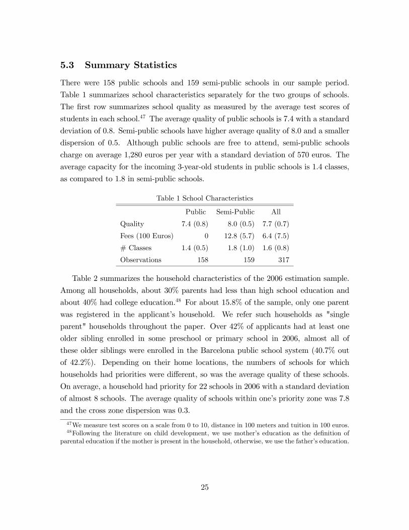
5.3 Summary Statistics

There were 158 public schools and 159 semi-public schools in our sample period.

Table 1 summarizes school characteristics separately for the two groups of schools.

The �rst row summarizes school quality as measured by the average test scores of

students in each school.47 The average quality of public schools is 7.4 with a standard

deviation of 0.8. Semi-public schools have higher average quality of 8.0 and a smaller

dispersion of 0.5. Although public schools are free to attend, semi-public schools

charge on average 1,280 euros per year with a standard deviation of 570 euros. The

average capacity for the incoming 3-year-old students in public schools is 1.4 classes,

as compared to 1.8 in semi-public schools.

Table 1 School Characteristics

Public Semi-Public All

Quality 7.4 (0.8) 8.0 (0.5) 7.7 (0.7)

Fees (100 Euros) 0 12.8 (5.7) 6.4 (7.5)

# Classes 1.4 (0.5) 1.8 (1.0) 1.6 (0.8)

Observations 158 159 317

Table 2 summarizes the household characteristics of the 2006 estimation sample.

Among all households, about 30% parents had less than high school education and

about 40% had college education.48 For about 15.8% of the sample, only one parent

was registered in the applicant�s household. We refer such households as "single

parent" households throughout the paper. Over 42% of applicants had at least one

older sibling enrolled in some preschool or primary school in 2006, almost all of

these older siblings were enrolled in the Barcelona public school system (40.7% out

of 42.2%). Depending on their home locations, the numbers of schools for which

households had priorities were di¤erent, so was the average quality of these schools.

On average, a household had priority for 22 schools in 2006 with a standard deviation

of almost 8 schools. The average quality of schools within one�s priority zone was 7.8

and the cross zone dispersion was 0.3.

47We measure test scores on a scale from 0 to 10, distance in 100 meters and tuition in 100 euros.48Following the literature on child development, we use mother�s education as the de�nition of

parental education if the mother is present in the household, otherwise, we use the father�s education.

25

Table 2 Household Characteristics

Parental Edua< HS 29.8%

Parental Edu = HS 30.4%

Parental Edu �College 39.8%

Single Parent 15.8%

Have school-age older sibling(s) 42.2%

# Schools in Zone 22.3 (7.9)

Average school quality in zone 7.8 (0.3)

Observations 6,836aParental Edu: mother�s edu if she is present, o/w father�s edu.

Table 3 shows the number of schools households listed on their application forms.

Households were allowed to list up to 10 schools, but most of households listed no

more than 3 schools, with 47% of households listing only one school. Across di¤erent

educational groups, parents with lower-than-high-school education were more likely to

have a shorter list, while parents with exact high school education tended to list more

schools than the others. Single parents also tended to list more schools compared to

both-parent households.

Table 3 Number of Schools Listed (%)

1 2 3 4 or more

All 46.9 12.4 16.9 23.8

Parental Edu < HS 49.8 15.0 19.5 15.7

Parental Edu = HS 43.4 12.1 18.4 26.2

Parental Edu �College 47.4 10.6 13.9 20.1

Single-Parent 43.3 14.7 16.8 25.2

Table 4 shows the round at which households were assigned. By de�nition, a

household was assigned to its rth listed school if it was assigned in round r; and

remained unassigned if it failed to get in any of its listed schools. Ninety three

percent of households were assigned in the �rst round; 2.8% were assigned in the

second round and 2.7% were unassigned. Across educational groups, college-educated

parents were most likely to be assigned to their �rst choices (93.7%), followed by the

lowest educational group. High-school educated parents were the least likely to be

assigned to their �rst choice and to be assigned at all. Single parents were more likely

to be assigned to their �rst choice compared to their counterpart.

26

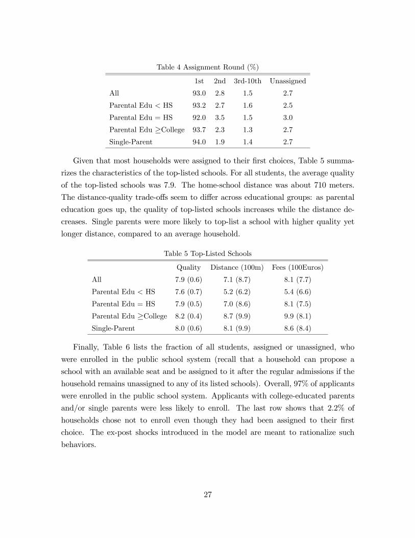
Table 4 Assignment Round (%)

1st 2nd 3rd-10th Unassigned

All 93.0 2.8 1.5 2.7

Parental Edu < HS 93.2 2.7 1.6 2.5

Parental Edu = HS 92.0 3.5 1.5 3.0

Parental Edu �College 93.7 2.3 1.3 2.7

Single-Parent 94.0 1.9 1.4 2.7

Given that most households were assigned to their �rst choices, Table 5 summa-

rizes the characteristics of the top-listed schools. For all students, the average quality

of the top-listed schools was 7.9. The home-school distance was about 710 meters.

The distance-quality trade-o¤s seem to di¤er across educational groups: as parental

education goes up, the quality of top-listed schools increases while the distance de-

creases. Single parents were more likely to top-list a school with higher quality yet

longer distance, compared to an average household.

Table 5 Top-Listed Schools

Quality Distance (100m) Fees (100Euros)

All 7.9 (0.6) 7.1 (8.7) 8.1 (7.7)

Parental Edu < HS 7.6 (0.7) 5.2 (6.2) 5.4 (6.6)

Parental Edu = HS 7.9 (0.5) 7.0 (8.6) 8.1 (7.5)

Parental Edu �College 8.2 (0.4) 8.7 (9.9) 9.9 (8.1)

Single-Parent 8.0 (0.6) 8.1 (9.9) 8.6 (8.4)

Finally, Table 6 lists the fraction of all students, assigned or unassigned, who

were enrolled in the public school system (recall that a household can propose a

school with an available seat and be assigned to it after the regular admissions if the

household remains unassigned to any of its listed schools). Overall, 97% of applicants

were enrolled in the public school system. Applicants with college-educated parents

and/or single parents were less likely to enroll. The last row shows that 2.2% of

households chose not to enroll even though they had been assigned to their �rst

choice. The ex-post shocks introduced in the model are meant to rationalize such

behaviors.

27

Table 6 Enrollment in Public System (%)

All 96.7

Parental Edu < HS 97.0

Parental Edu = HS 97.1

Parental Edu �College 96.3

Single-Parent 96.1

Assigned in Round 1 97.8

6 Results

6.1 Parameter Estimates

Table 7 presents the estimated parameters governing household preferences, with

standard errors shown in parentheses. The utility function is linear with interactions

between household characteristics and school characteristics. We treat high-school

educated both-parent households as the base group. High-school educated parents

value schools within the public school system more than other educational groups,

especially the college-educated group. One explanation is that college-educated par-

ents are more likely to be able to a¤ord a costly outside option (a private school).

Single parents also tend to value public schools less than their counterpart. The next

row shows that it is especially attractive for a household to send the child to the

same school where her older sibling was enrolled in. These parameter estimates are

consistent with the observed behaviors. For example, Table 5 and Table 6 show that

although college-educated parents and single parents were more likely to be assigned

to their top choices, they were less likely to enroll their children in the public school

system. It is also observed that most households with more than one child sent the

younger child to her sibling�s school.

The sixth row on the left panel of Table 7 shows that holding everything else

constant, semi-public schools are more preferable to public schools, which may re�ect

the fact parents value the more �exible management and curriculum in semi-public

schools. The next four rows show the e¤ect of school fees. Price sensitivities decrease

with education levels; and the cost of fees is concave. In particular, the cost of

fees peaks around 1,500 (1,600) euros per year for the college (high-school) educated

parents, which is around the 75th percentile of the distribution of fees charged by semi-

28

public schools. For the lowest-education group, the cost peaks around 2,100 euros,

which is the 95th percentile of of the distribution of fees charged by semi-public schools.

The �nding that tuition cost is concave re�ects the fact that a large part of the fees are

charged for additional services provided by semi-public schools, which apparently are

valued by parents. Our preference parameters on fees capture the e¤ects of monetary

costs net of the bene�ts associated with these fees.49 The last three rows on the

left panel show households�additional preferences for schools with capacities of more

than one �rst-year class. Consistent with the fact that larger schools tend to have

more resources and lower closing-down probabilities, our parameter estimates show

that households prefer schools with larger capacity.

Table 7 Preference Parameters

Constant 3478.9 (122.4) q*I(Edu < HS) 0.01 (1.87)

Single Parent -261.9 (172.6) q*I(Edu = HS) 6.4 (0.4)

Education < HS -57.7 (471.3) q*I(Edu > HS) 1.6 (0.2)

Education > HS -405.6 (150.7) I (q > qg)*(q � qg)2*I(Edu < HS) 7.8 (3.1)

Sibling School 1618.7 (194.5) I (q > qg)*(q � qg)2*I(Edu = HS) 20.6 (1.3)

Semi-Public School 37.6 (0.3) I (q > qg)*(q � qg)2*I(Edu > HS) 41.6 (0.2)

Fee*I(Edu < HS) -5.1 (0.04) I�q < qb

�*�qb � q

�2-10.6 (0.2)

Fee*I(Edu = HS) -3.8 (0.01) Distance (100m) -1 (n/a)

Fee*I(Edu > HS) -3.6 (0.01) Distance2 -0.05 (0.001)

Fee2 0.12 (0.001) Distance>5 (100m) -46.3 (0.1)

# Classes= 2 22.0 (0.1) Distance>10 (100m) -23.5 (0.3)

# Classes= 3 40.7 (0.4) ��(taste dispersion) 53.8 (0.1)

# Classes> 3 54.2 (0.4) ��(post-application shock) 2131.7 (40.6)

qg(qb) is the quality of the school at the 75th (25th) percentile.

The right panel of Table 7 shows the trade-o¤s between quality (q) and distance.

There are three sets of quality parameters: 1) education-group-speci�c linear impacts

of quality, 2) education-group-speci�c square terms on school quality beyond the 75th

percentile of the quality distribution (qg) ; and 3) a square term on school quality below

the 25th percentile�qb�: Except for the high-school-educated parents, the linear e¤ects

49It will be interesting to disentangle the cost from the bene�ts associated with service fees, whichrequires information that is unavailable in our data sets.

29

of school quality are small, especially for the lowest-educational group, for whom the

linear term is almost zero. Households do, however, value the top schools. As shown

in the 4th to 6th row, the preferences for schools that are ranked at the higher end

of the quality distribution are strongly convex, especially for the higher educated

groups. The next row shows that households also have a strong aversion against

schools at the lower end of the quality distribution. In sum, although households

may not care too much about the quality di¤erences across schools in the middle of

the quality distribution, they do care much more about the very good schools and

the very bad ones. The next four rows show preferences on distances. The linear

preference parameter on distance is normalized to -1. The cost of distance is convex

with the square term being 0.05. In addition, we allow two jumps in the cost of

distances. The �rst jump is set at 500 meters, which is meant to capture an easy-to-

walk distance even for the 3-year old. Another jump is at the 1 kilometer threshold,

which is a long yet perhaps still manageable walking distance. As households may

have to rely on some other transportation methods when a school is beyond walking

distances, it is not surprising to see that the cost of distance jumps signi�cantly at the

thresholds, by about 4.6 kilometers at the �rst threshold and by another 2.3 kilometers

at the second. Our �ndings that parents of di¤erent education levels di¤er in their

views of the trade-o¤s among quality, fees and distance are consistent with those

in the literature.50 Finally, the last two rows on the right panel show, respectively,

the dispersion of household preferences across schools and that of post-application

shocks. The latter is necessary to rationalize the fact that some households gave up

their �rst choices after being assigned. In addition, households take expectations over

these ex-post shocks when applying, thus application provides another bene�t, i.e.,

an option value.

Table 8 presents the estimated parameters governing the probability that a house-

hold is strategic, which takes a logistic functional form. Single parents are slightly

less likely to be strategic. Compared to high-school-educated parents, those with

lower or higher education levels are more likely to be strategic. We do not �nd that

strategic households are more likely to live in zones with more schools, and in fact,

the coe¢ cient is slightly negative. However, we do �nd that strategic households are

more likely to live in zones with higher average school quality. Although not precisely

50For example, Burgess et al (2009), Hastings, Kane and Staiger (2008), He (2012) and Abdulka-diro¼glu, Agarwal and Pathak (2014).

30

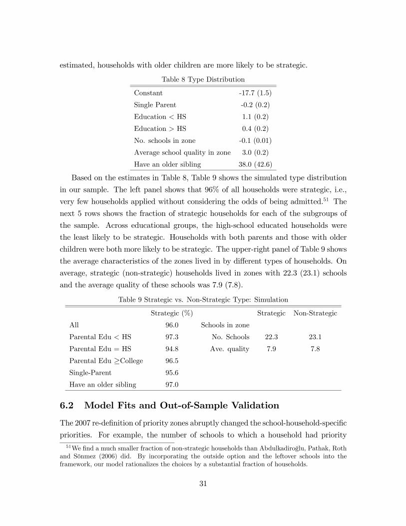
estimated, households with older children are more likely to be strategic.

Table 8 Type Distribution

Constant -17.7 (1.5)

Single Parent -0.2 (0.2)

Education < HS 1.1 (0.2)

Education > HS 0.4 (0.2)

No. schools in zone -0.1 (0.01)

Average school quality in zone 3.0 (0.2)

Have an older sibling 38.0 (42.6)

Based on the estimates in Table 8, Table 9 shows the simulated type distribution

in our sample. The left panel shows that 96% of all households were strategic, i.e.,

very few households applied without considering the odds of being admitted.51 The

next 5 rows shows the fraction of strategic households for each of the subgroups of

the sample. Across educational groups, the high-school educated households were

the least likely to be strategic. Households with both parents and those with older

children were both more likely to be strategic. The upper-right panel of Table 9 shows

the average characteristics of the zones lived in by di¤erent types of households. On

average, strategic (non-strategic) households lived in zones with 22.3 (23.1) schools

and the average quality of these schools was 7.9 (7.8).

Table 9 Strategic vs. Non-Strategic Type: Simulation

Strategic (%) Strategic Non-Strategic

All 96.0 Schools in zone

Parental Edu < HS 97.3 No. Schools 22.3 23.1

Parental Edu = HS 94.8 Ave. quality 7.9 7.8

Parental Edu �College 96.5

Single-Parent 95.6

Have an older sibling 97.0

6.2 Model Fits and Out-of-Sample Validation

The 2007 re-de�nition of priority zones abruptly changed the school-household-speci�c

priorities. For example, the number of schools to which a household had priority51We �nd a much smaller fraction of non-strategic households than Abdulkadiro¼glu, Pathak, Roth

and Sönmez (2006) did. By incorporating the outside option and the leftover schools into theframework, our model rationalizes the choices by a substantial fraction of households.

31

became 7.0 on average with a standard deviation of 1.5 in 2007, as compared to

the 22.3 (7.9) �gure in 2006. More importantly, the priority schools became those

that surrounded each home location, which also changed the risk-quality-distance

trade-o¤s faced by households. In this section, we show the model �ts for both the

2006 and the 2007 samples.52 To simulate the 2007 outcomes, we �rst calculate

the admissions probabilities in 2007 via the same procedure as we do for the year

2006, using the entire 2007 sample. Then we use the selected 2007 sample of 7,437

households to conduct an out-of-sample validation, where the sample selection rule is

the one used for the 2006 sample.53 To the extent that the change came as a surprise

to households, it is reasonable to believe households had been unable to reallocate

before submitting their applications in 2007. As such, we simulate the distribution

of 2007 household types using the characteristics of their residential zones according

to the 2006 de�nition.54

Considered as the most informative test of the model, the �rst two rows of Table

10 explore the changes in the de�nition of priority zones.55 The 2007 reform led to

situations where some schools were in the priority zone for a household in one year but

not in the other, which would a¤ect the behavior of a strategic household. As shown

in the �rst row of Table 10, in 2006, 24% of the households in our sample top-listed

a school that was in their priority zone by the 2006 de�nition but not by the 2007

de�nition. In 2007, the fraction of households that top listed these schools dropped

to 12%. On the other hand, the second row of Table 10 shows that the fraction of

households that top-listed schools in their priority zone only by the 2007 de�nition

but not by the 2006 de�nition increased from 3% to 12% over the two years. The

model is able to replicate such behaviors and predicts the changes as being from 22%

to 15% for the �rst case, and from 5.7% to 11.2% for the second case. The next 3

rows of Table 10 show that the model �ts the data well in terms of the characteristics

of the top-listed schools, including average quality, distances and fees. In particular,

52Appendix Table A1-A6 show the �ts for subgroups of households conditional on demographics.53In 2007, 12,335 Barcelona households participated. We follow the same sample selection rule as

that for the 2006 sample. In particular, the 7,437 households in 2007 do not include the 998 parentswho reported "high school or above" as their education levels. We interpolate the probability ofbeing college-educated for these parents and include them in the counterfactual policy experiments.54As shown below, we can �t the data in both years, suggesting that our assumption about

household type distribution in 2007 is a reasonable one.55Calsamiglia and Güell (2014) use this change to show that the observed application behavior

was driven largely by admissions priorities.

32

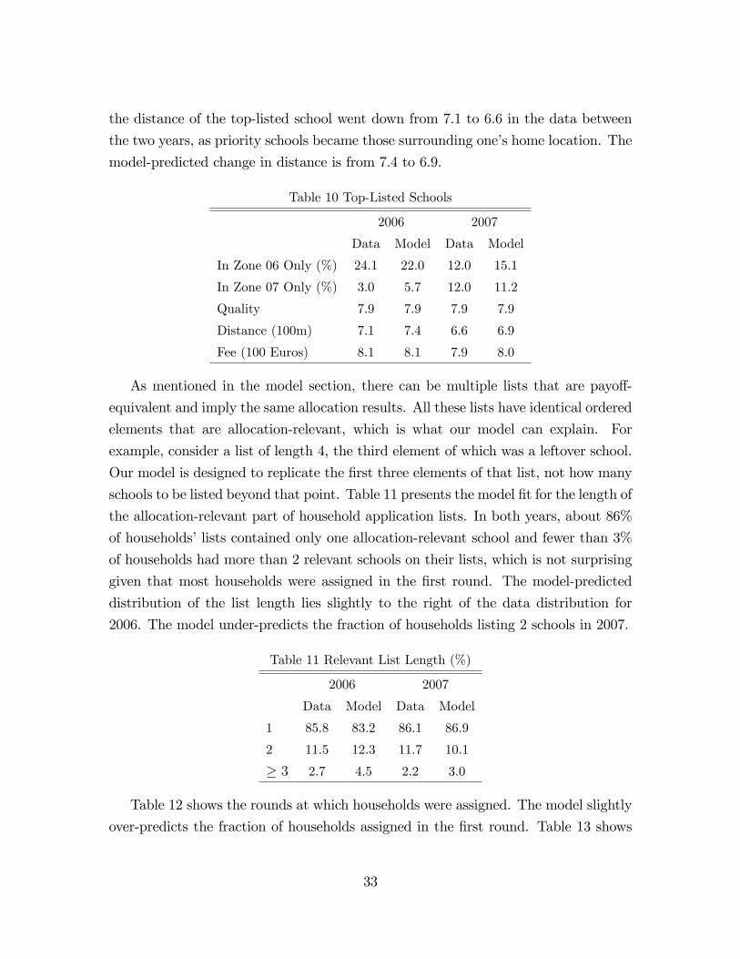
the distance of the top-listed school went down from 7.1 to 6.6 in the data between

the two years, as priority schools became those surrounding one�s home location. The

model-predicted change in distance is from 7.4 to 6.9.

Table 10 Top-Listed Schools

2006 2007

Data Model Data Model

In Zone 06 Only (%) 24.1 22.0 12.0 15.1

In Zone 07 Only (%) 3.0 5.7 12.0 11.2

Quality 7.9 7.9 7.9 7.9

Distance (100m) 7.1 7.4 6.6 6.9

Fee (100 Euros) 8.1 8.1 7.9 8.0

As mentioned in the model section, there can be multiple lists that are payo¤-

equivalent and imply the same allocation results. All these lists have identical ordered

elements that are allocation-relevant, which is what our model can explain. For

example, consider a list of length 4, the third element of which was a leftover school.

Our model is designed to replicate the �rst three elements of that list, not how many

schools to be listed beyond that point. Table 11 presents the model �t for the length of

the allocation-relevant part of household application lists. In both years, about 86%

of households�lists contained only one allocation-relevant school and fewer than 3%

of households had more than 2 relevant schools on their lists, which is not surprising

given that most households were assigned in the �rst round. The model-predicted

distribution of the list length lies slightly to the right of the data distribution for

2006. The model under-predicts the fraction of households listing 2 schools in 2007.

Table 11 Relevant List Length (%)

2006 2007

Data Model Data Model

1 85.8 83.2 86.1 86.9

2 11.5 12.3 11.7 10.1

� 3 2.7 4.5 2.2 3.0

Table 12 shows the rounds at which households were assigned. The model slightly

over-predicts the fraction of households assigned in the �rst round. Table 13 shows

33

that the model closely replicates the enrollment rate within the public school sys-

tem. In particular, with the ex-post shocks, the model replicates the non-enrollment

behavior by households who were assigned to their �rst choice.

Table 12 Assignment Round (%)

2006 2007

Data Model Data Model

1 93.0 94.3 92.0 94.5

2 2.8 2.3 3.1 2.0

� 3 1.5 0.2 1.8 0.4

Unassigned 2.7 3.2 3.1 3.1

Table 13 Enrollment in the Public System (%)

2006 2007

Data Model Data Model

All 96.7 96.5 97.6 96.5

Assigned in Round 1 97.8 96.7 98.3 97.1

7 BM vs. GS vs. TTC

Using the estimated model, we are ready to answer the question we posed at the

beginning of the paper. How does the current Boston mechanism (BM) compare

with two of its alternatives, the Gale-Shapley student deferred acceptance mecha-

nism (GS) and the top trading cycles mechanism (TTC)? In a di¤erent experiment,

presented in the appendix, we assess the impacts of the 2007 reform, which changed

the student-school priority structure by rede�ning priority zones. In both experi-

ments, households�welfare refers to their evaluations of their assignment outcomes

relative to their outside options, i.e., vij:56

7.1 Theoretical Background

This subsection brie�y discusses the properties of the three alternative mechanisms;

Appendix E contains detailed descriptions.57 The GS procedure is similar to BM56All simulations include the interpolated sample, as mentioned in footnotes 46 and 53. All

simulations use the school-household-speci�c priority scores given by (1) ; as they were de�ned bythe o¢ cial rules in the relevant year.57See Abdulkadiro¼glu and Sönmez (2003) for further theoretical discussions.

34

with the key di¤erences that students are only temporarily assigned to schools in

each round and that one�s chance of being �nally admitted to a school does not

depend on the ranking of the school on her application list. The TTC algorithm

has a very di¤erent structure. Intuitively, in each round TTC creates cycles of trade

between individuals. Each individual in a cycle trades o¤a seat in her highest-priority

school for a seat in her announced most preferred school among those that still have

seats. Whenever such a cycle is formed the allocation is �nal.

Three properties are considered as desirable for a mechanism, i.e., Pareto e¢ -

ciency, truth revealing and the elimination of justi�ed envy (also known as stabil-

ity).58 Unfortunately, all three properties may not hold simultaneously. BM satis�es

none of the properties. GS and TTC are both truth revealing. Between the other two

con�icting properties, GS eliminates justi�ed envy at the cost of Pareto e¢ ciency,

while TTC achieves Pareto e¢ ciency at the cost of stability.

Despite the fact that BM does not satisfy any of the three desirable properties,

the welfare comparison between BM and its alternatives is ambiguous.59 The am-

biguity arises from the coexistence of two competing forces. On the one hand, BM

can lead to potential misallocations because households hide their true preferences.

This source of misallocation is absent in the truth-revealing GS and TTC. On the

other hand, BM may better "respect" households�cardinal preferences than GS and

TTC (Abdulkadiro¼glu, Che and Yasuda (2011)). BM-induced household behaviors

increase the chance that the "right match" is formed, where a school being matched

to households that value it more.60 Under a truth-revealing mechanism, households

who share the same ordinal preferences will rank schools the same way in their appli-

cations and be given the same chance of being allocated to various schools, regardless

58Stability requires that there be no unmatched student-school pair (i; s) where student i prefersschool s to her assignment and she has higher priority than some other student who is assigned aseat at school s.59The ambiguity has been re�ected in the con�icting �ndings in the theoretical and lab experi-

mental studies that compare BM with GS. Pareto e¢ ciency is an ordinal concept, which does notnecessarily imply the highest level of total household welfare.60The intuition can be explained by the following simple example with equal priorities. Consider

three schools and a set of households who share the same ordinal but di¤erent cardinal preferencesfor these schools, where the schools are ranked from high to low as Schools 1, 2 and 3. Under BM,the strategic decision is whether to take the high risk and top-list School 1 or to play it safe andtop-list School 2. Given the same evaluation for School 1, a household whose evaluations for Schools2 and 3 are similar is more likely to choose the risky strategy because it has less to lose from thegamble. Given the same evaluation for School 3, a household that values School 1 much higher thanSchool 2 is more likely to choose the risky strategy because it has more to gain from the gamble.

35

of who will gain the most from each school. Given that it is theoretically inconclusive,

the welfare comparison between BM and GS or TTC becomes an empirical question,

one that we answer below.

7.2 Results

Under both GS and TTC, all households, strategic or not, will list schools according

to their true preferences. As such, we simulate each household�s application list

according to their true preferences and assign them using GS and then using TTC.61

We compare the results from these two counterfactual mechanisms with those from

the baseline.62 We present our results under the more recent, i.e., the 2007, priority

zone structure.63

Remark 4 In the following, we will present consequences of the reforms from BM

to GS and TTC on the total household welfare, the distribution of winners and losers

among di¤erent subgroups of households, as well as the assignment outcomes. No-

tice that the level of total household welfare is not necessarily the criterion for social

welfare, which may involve di¤erent weights across households. Given that we can

calculate the welfare changes at the household level, our results can be used to cal-

culate any weighted social welfare. Moreover, household welfare may not be the only

factor that policy makers consider. For example, policy makers may put high value on

truth-revealing and the elimination of justi�ed envy, which will make GS particularly

attractive. Therefore, we do not necessarily recommend one mechanism over another

in this paper. However, given a social objective, our results can easily be used for

policy-making purposes.

7.2.1 Household Welfare Comparison

To form the basis for comparison, the �rst column of Table 14 shows the average

welfare and the standard deviations among the population (in parentheses) under BM.

61Notice that all allocation mechanisms we consider use random lotteries to rank students withthe same priority score. As such, for each experiment we simulate the overall allocation procedureand obtain the outcomes for all students for a given set of random lotteries. We repeat this processmany times to obtain the expected (average) outcomes for each simulated student.62Notice that to simulate GS and TTC, it is su¢ cient to know household preferences. However,

to compare GS or TTC with the baseline (Boston) mechanism, one needs to know the distributionof household strategic types.63The 2006 results are similar, available on request.

36

The second column of Table 14 shows changes in welfare (�utils) when BM is replaced

by GS. The average household welfare is decreased by 2.7 from the BM level of 4,146.

Moreover, the average welfare decreases among all subgroups of households, as de�ned

by strategic sophistication or education levels.64 To translate the welfare changes

into more intuitive measures, we ask the following question:"Holding everything else

constant at the baseline level, what is the adjustment in attendance fees that will bring

a household�s welfare from its level under BM to its level under the counterfactual

(new) system?". Let �feesi denote the welfare-equalizing fee adjustment for household

i:65 Notice that a negative �feesi implies an increase in welfare.

Table 14 Household Welfare: BM vs. GS vs. TTC

% BM GS-BM TTC-BM

�utils �fees �utils �fees

All 4,146 (752) -2.7 (23.5) 59.9 (543.0) 1.4 (33.2) -88.0 (581.3)

Strategic 4,145 (753) -2.6 (23.4) 57.4 (540.1) 1.4 (32.8) -88.6 (580.9)

Non-strategic 4,173 (752) -5.5 (27.4) 116.8 (603.7) 0.1 (40.4) -75.5 (591.4)

Edu<HS 4,141 (722) -4.5 (22.4) 152.6 (510.0) 1.9 (24.9) -7.4 (478.0)

Edu= HS 4,308 (736) -2.6 (26.2) 53.3 (576.6) 1.4 (36.3) -106.6 (634.4)

Edu�College 4,022 (760) -1.6 (22.0) 3.2 (528.5) 1.1 (35.4) -127.1 (594.7)

Column 3 of Table 14 reports the average welfare-equalizing fee adjustments. Av-

eraging over all households, the change from BM to GS causes a welfare loss that

is equivalent to a 60-euro increase in school fees, with a 543-euro standard devia-

tion across the population. Average non-strategic households su¤er more, with a loss

equivalent to a 117-euro increase in fees. The average loss among the lowest education

group is equivalent to a 153-euro increase in fees, while the highest education group

su¤ers the least.64Our �nding that GS decreases welfare for both strategic and non-strategic households is consis-

tent with some recent theoretical work, e.g., Abdulkadiro¼glu, Che, and Yasuda (2011).65Formally, let j be the school household i is assigned to under BM and vij =

� ( ewj ; feej ; xi; dij ; �ij) be i�s value of being assigned to j, where ewj is the vector of school j�s char-acteristics excluding the annual fees (feej); let vijnew be household i�s welfare under the new (GSor TTC) system which assigns i to school jnew. For each household, de�ne the welfare-equalizingfee adjustment �feesi as the solution to the following equation

�� ewj ; feej +�feesi ; xi; dij ; �ij

�= vijnew :

Notice that for some households, the adjustment may make the fee negative, leading to positive cashtransfers to households.

37

The last two columns of Table 14 compares BM with TTC. For an average house-

hold, the change from BM into TTC increases the welfare by an amount equivalent

to decreasing school fees by 88 euros. As such, TTC leads to the highest total house-

hold welfare among all three alternatives. Moreover, the average welfare increases

within each subgroup of households, with strategic households gaining more than non-

strategic households and higher-education groups gaining more than lower-education

groups.

Result 1: In terms of the level of total household welfare, the three mechanisms areranked as TTC > BM > GS.

Winners and Losers We next present the e¤ects by distinguishing between win-

ners and losers. Table 15 focuses on fractions of winners and losers under each change.

The �rst two columns show the case for a change from BM to GS, which bene�ts fewer

than 10% of households while hurting over 28% of them. Moreover, the fact that there

are more losers than winners holds for all subgroups of households. In contrast, as

shown in Columns 3 and 4, a change from BM to TTC generates more winners

(20.4%) than losers (18.9%), which again persists across all subgroups of households.

Table 16 shows the welfare changes among winners and among losers.66 Under both

counterfactual scenarios, the magnitude of gains among winners is larger than that

of losses among losers. From BM to GS (from BM to TTC), an average winner gains

by an amount equivalent to a 872-euro (804-euro) decrease in school fees, while the

average loser loses by a 502-euro (408-euro) increase in fees.

Result 2: There are more losers than winners from a change of BM into GS, and

more winners than losers from a change of BM into TTC.

Table 15 Winners and Losers (%)

BM to GS BM to TTC

Winner Loser Winner Loser

All 9.5 28.5 20.4 18.9

Strategic 9.6 28.2 20.5 18.8

Non-strategic 8.6 35.4 19.7 22.0

Edu < HS 8.5 31.3 20.9 18.1

Edu = HS 10.9 31.2 22.5 21.0

Edu �College 9.2 24.4 18.5 17.8

66Appendix Tables A7-A8 show the same statistics for subgroups of households.

38

Table 16 Gains and Losses

BM to GS BM to TTC

�utils �fees �utils �fees

Winner 35.3 (45.0) -872.2 (775.0) 30.7 (40.8) -804.0 (743.8)

Loser -21.3 (20.5) 502.1 (578.7) -25.7 (48.6) 408.4 (597.5)

7.2.2 Cross-Zone Inequality

A household�s welfare can be signi�cantly a¤ected by the school quality within its zone

not only because of the quality-distance trade-o¤, but also because of the quality-risk

trade-o¤ created by the priority structure. For equity concerns, a replacement of BM

will be more desirable if it is more likely to bene�t those living in poor-quality zones.

Table 17 tests whether or not each of the counterfactual reforms meets this goal by

showing the zone quality among winners and losers from each reform. The �rst two

columns show the case for the change from BM to GS. The winners are those who

live in better zones than the losers: the average zone quality among all winners is

7.75 while that among losers is 7.65. As shown in the next three rows, this pattern

persists across all educational groups. Therefore, a change from BM to GS increases

the dependence of welfare on zone quality, which is against the goal of equity across

zones. The next two columns show that changing from BM to TTC, the average

zone quality is similar across winners and losers, which implies that such a reform is

unlikely to reduce or to enlarge the cross-zone inequality as compared to BM.

Result 3: Welfare dependence on zone quality increases with a change from BM to

GS, and remains una¤ected by a change from BM to TTC.

Table 17 Zone Quality: Winners vs. Losers

BM to GS BM to TTC

Winner Loser Winner Loser

All 7.75 7.65 7.70 7.71

Edu < HS 7.57 7.48 7.52 7.51

Edu = HS 7.72 7.65 7.69 7.69

Edu �College 7.88 7.80 7.84 7.85

The Cost of the Elimination of Justi�ed Envy Underlying the results in Table

17 is the residence-based priority and the high respect GS has for priorities, the

39

latter enabling GS to eliminate justi�ed envy but not without cost.67 The �rst three

columns of Table 18 show the fractions of households assigned to schools in their own

school zones under alternative mechanisms. The �rst row shows that about 70% of

all households are assigned to schools in zone under GS, followed by the case of BM

(65%) and �nally TTC (58%). The second row shows this fraction among households

whose favorite schools are in their school zones. While over 95% of these households

are assigned to in-zone schools under BM and GS, this �gure is only 90% under TTC.

Most illustrative of the point, the third row shows this fraction among households

whose favorite schools are out of their school zones. Even though a household would

like to attend a school out of its zone, due to its high respect for priorities, GS assigns

30% of them within their zone, as compared to 20% under BM and 10% under TTC.

Table 18 The Cost of the Elimination of Justi�ed Envy

Assigned in Zone (%) Assigned to Favorite (%)

BM GS TTC BM GS TTC

All Households 65.5 69.7 58.5 79.4 75.0 80.7

Favorite is in Zone 95.3 95.4 89.9 92.6 89.8 83.8

Favorite is out of Zone 19.5 30.0 10.0 58.9 52.0 76.0

The last three columns of Table 18 shows the extent to which the respect for

priorities hampers households� chances of being assigned to their favorite schools.

Row 1 shows that over all households, the chance of being assigned to their favorite

schools is the highest under TTC (81%) and lowest under GS (75%). Row 2 shows

that BM is the best at accommodating households preferences if their favorite schools

are in their school zones, followed by GS and then TTC. Finally, while TTC enables

76% of households whose favorite schools are out of their zones to attend their favorite

schools, this fraction decreases to 59% under BM and 52% under GS.

67Under BM, a risk-taking poor-zone household only needs to compete with other householdswho top-listed the same school, since the assignment is �nal at each round. Under GS, the samepoor-zone household has to compete not only with those who have the same favorite school butalso with those who are unable to get their favorite schools, because the assignment in each roundis only temporary. This can make it harder for a poor-zone household to get into a better schoolout of its zone under GS than under BM, which in turn can make such a household worse o¤ underGS. Under TTC, having high priority to a better school increases one�s chance to form a tradingcycle. However, conditional on forming a cycle, the assignment does not depend one�s priority forthe receiving school. Therefore, who wins and who loses from the change of BM into TTC dependsmuch less on the quality of one�s own zone. See the appendix for the details of the GS and the TTCalgorithms.

40

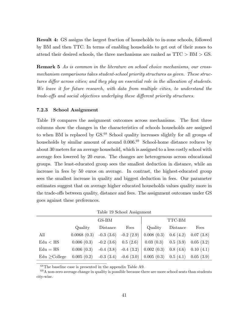
Result 4: GS assigns the largest fraction of households to in-zone schools, followedby BM and then TTC. In terms of enabling households to get out of their zones to

attend their desired schools, the three mechanisms are ranked as TTC > BM > GS.

Remark 5 As is common in the literature on school choice mechanisms, our cross-mechanism comparisons takes student-school priority structures as given. These struc-

tures di¤er across cities; and they play an essential role in the allocation of students.

We leave it for future research, with data from multiple cities, to understand the

trade-o¤s and social objectives underlying these di¤erent priority structures.

7.2.3 School Assignment

Table 19 compares the assignment outcomes across mechanisms. The �rst three

columns show the changes in the characteristics of schools households are assigned

to when BM is replaced by GS.68 School quality increases slightly for all groups of

households by similar amount of around 0.006.69 School-home distance reduces by

about 30 meters for an average household, which is assigned to a less costly school with

average fees lowered by 20 euros. The changes are heterogenous across educational

groups. The least-educated group sees the smallest deduction in distance, while an

increase in fees by 50 euros on average. In contrast, the highest-educated group

sees the smallest increase in quality and biggest deduction in fees. Our parameter

estimates suggest that on average higher educated households values quality more in

the trade-o¤s between quality, distance and fees. The assignment outcomes under GS

goes against these preferences.

Table 19 School Assignment

GS-BM TTC-BM

Quality Distance Fees Quality Distance Fees

All 0.0068 (0.3) -0.3 (3.6) -0.2 (2.9) 0.008 (0.3) 0.6 (4.2) 0.07 (3.8)

Edu < HS 0.006 (0.3) -0.2 (3.6) 0.5 (2.6) 0.03 (0.3) 0.5 (3.9) 0.05 (3.2)

Edu = HS 0.006 (0.3) -0.4 (3.8) -0.4 (3.2) 0.002 (0.3) 0.8 (4.6) 0.10 (4.1)

Edu �College 0.005 (0.2) -0.3 (3.4) -0.6 (3.0) 0.005 (0.3) 0.5 (4.1) 0.05 (3.9)

68The baseline case is presented in the appendix Table A9.69A non-zero average change in quality is possible because there are more school seats than students

city-wise.

41

The last three columns of Table 19 show the changes when BM is replaced by

TTC. School quality increases by 0.008 on average, with the lowest-educational group

experiencing the biggest increase of 0.03. School-home distance increases by about

60 meters for an average household. As an illustration of the misallocation arising

from people hiding their true preferences under BM, Table 19 shows that the current

BM makes households ine¢ ciently apply for close-by schools that they have higher

priority for, while giving up higher-quality schools with longer distance that they have

lower priority for.

Result 5: Compared to TTC, both BM and GS ine¢ ciently assign students to

schools that are of shorter distance but lower quality.

8 Conclusion

We have developed and estimated a model of school choices by households under the

Boston mechanism. We have recovered the joint distribution of household preferences

and their strategic vs. non-strategic types, using administrative data from Barcelona

before a drastic change in the de�nition of households�priority school zones. The

estimated model has been validated using data after this drastic change.

We contribute to the on-going debates on school choice mechanism designs by

quantifying the welfare impacts of replacing the Boston mechanism with its two al-

ternatives, GS and TTC. A change from the Boston mechanism to GS creates more

losers than winners. This change also increases the dependency of a household�s wel-

fare on the quality of its school zones, leading to further inequality concerns across

residential zones. In contrast, a change from the Boston mechanism to TTC creates

more winners than losers. However, the change of BM to TTC is unlikely to reduce

or to enlarge the cross-zone inequality.

The methods developed in this paper and the main empirical �ndings are promis-

ing for future research. One particularly interesting extension is to incorporate house-

hold�s residential choices into the framework of this paper. Individual households may

relocate in order to take advantage of changes in school choice mechanisms and/or in

residence-based priority structures. Such individual incentives will in turn a¤ect the

housing market. There is a large literature on the capitalization of school quality for

housing prices, as reviewed by Black and Machin (2010) and Gibbons and Machin

42

(2008).70 An important yet challenging research project involves combining this litera-

ture and the framework proposed in our paper, in order to form a more comprehensive

view of the equilibrium impacts of school choice mechanisms on households�choices

of schools and residential areas, and on the housing market.

References

Abdulkadiro¼glu, A., N. Agarwal and P. Pathak (2014). "The Welfare E¤ects of Con-

gestion in Uncoordinated Assignment: Evidence from the NYC HS Match," NBER

working paper.

Abdulkadiroglu, A., J. Angrist, S. Dynarski, T. Kane, and P. Pathak (2011). �Ac-

countability and Flexibility in Public Schools: Evidence from Boston�s Charters and

Pilots,�Quarterly Journal of Economics, 126(2): 699�748.

Abdulkadiro¼glu, A., Y. Che, and Y. Yasuda (2011). "Resolving Con�icting Prefer-

ences in School Choice: the Boston Mechanism Reconsidered," American Economic

Review, 101(1): 399-410.

Abdulkadiro¼glu, A., P. Pathak, and A. Roth (2009). �Strategy-Proofness versus Ef-

�ciency in Matching with Indi¤erences: Redesigning the NYC High School Match.�

American Economic Review, 99(5): 1954�78.

Abdulkadiro¼glu, A., P. Pathak, A. Roth and T. Sönmez (2005). "The Boston Public

School Match," American Economic Review, Papers and Proceedings, 95(2): 368-371.

Abdulkadiro¼glu, A., P. Pathak, A. Roth and T. Sönmez (2006). "Changing the Boston

School Choice Mechanism: Strategy-proofness as Equal Access," National Bureau of

Economic Research Working Paper 11965.

Abdulkadiro¼glu, A., and T. Sönmez (2003). "School Choice: A Mechanism Design

Approach," American Economic Review, 93(3): 729-747.

70Ries and Somerville (2010) exploit changes in the catchment areas of public schools in Vancouverand �nd signi�cant e¤ects of school performance on housing prices. Epple and Romano (2003)conjecture that school choice systems can eliminate the capitalization of school quality on the housingmarket. Machin and Salvanes (2010) exploit policy reforms in Oslo that allowed students to attendschools without having to live in the school�s catchment area, and �nd a signi�cant decrease in thecorrelation between a school�s quality and housing prices.

43

Agarwal, N. and P. Somaini (2014). "Demand Analysis Using Strategic Reports: An

Application to a School Choice Mechanism," Working Paper MIT.

Bajari, P. and A. Hortacsu (2005) "Are Structural Estimates of Auction Models

Reasonable? Evidence from Experimental Data," Journal of Political Economy 113,

703�741.

Black, S. and S. Machin (2010) �Housing Valuations of School Performance� in E.

Hanishek, S. Machin and L. Woessmann (eds.), Handbook of the Economics of Edu-

cation, Amsterdam: Elsevier.

Blume, L., W. Brock, S. Durlauf and Y. Ioannides (2011). "Identi�cation of Social

Interactions," Handbook of Social Economics, ed. by J. Benhabib, A. Bisin and M.

Jackson, North-Holland, Vol 1B: 853-964.

Burgess, S., E. Greaves, A. Vignoles and D. Wilson (2009). "Parental Choice of

primary school in England: what type of schools do parents choose?" CMPOWorking

Paper No. 09/224.

Calsamiglia, C., M. Güell (2014). �The Illusion of Choice: Evidence from Barcelona,�

CEPR Discussion Paper 10011.

Calsamiglia, C. and Miralles A. (2014). �All about priorities? Less choice with bad

schools,�mimeo UAB.

Chen, Y., and T. Sönmez (2006). "School Choice: An Experimental Study," Journal

of Economic Theory, 127(1): 202-231.

Deming, D., J. Hastings, T. Kane, and D. Staiger (2014). �School Choice, School

Quality and Postsecondary Attainment,�American Economic Review, 104(3): 991�

1013.

Epple, D. and R. Romano (2003). "Neighborhood Schools, Choice, and the Distrib-

ution of Educational Bene�ts," in C. Hoxby (ed), The Economics of School Choice,

University of Chicago Press.

Epple, D. and R. Romano (2011). "Peer e¤ects in education : a survey of the theory

and evidence," Handbook of Social Economics, ed. by J. Benhabib, A. Bisin and M.

Jackson, North-Holland, Vol 1B: 1053-1163.

44

Ergin, H., and T. Sönmez (2006). �Games of School Choice under the Boston Mech-

anism," Journal of Public Economics, 90(1-2): 215-237.

Featherston, C. and M. Niederle (2008). "Ex Ante E¢ ciency in School Choice Mech-

anisms: An Experimental Investigation," NBER Working Paper 14618.

Fu, C. (2014). "Equilibrium Tuition, Applications, Admissions and Enrollment in the

College Market," Journal of Political Economy, 122(2): 225-281.

Gibbons, S. and S. Machin (2008) �Valuing School Quality, Better Transport and

Lower Crime," Oxford Review of Economic Policy, 24: 99-119.

Hastings, J., T. Kane and D. Staiger (2009). "Heterogeneous Preferences and the

E¢ cacy of School Choice," NBER Paper Working Paper 12145.

Hastings, J. and J. Weinstein (2008) �Information, School Choice and Academic

Achievement: Evidence from Two Experiments," Quarterly Journal of Economics,

1373-1414.

He, Y. (2012). "Gaming the Boston School Choice Mechanism in Beijing," Working

Paper, Toulouse School of Economics.

Hwang, S. (2014). "A Robust Redesign of High School Match," Working Paper, Uni-

versity of Chicago.

Jensen, R. (2010). �The (Perceived) Returns to Education and the Demand for

Schooling," Quarterly Journal of Economics, 125 2, 515-548.

Keane, M. and R. Mo¢ tt (1998). "A Structural Model of Multiple Welfare Program

Participation and Labor Supply." International Economic Review 39, 553�590.

Keane, M., P. Todd and K. Wolpin (2011) "The Structural Estimation of Behavioral

Models: Discrete Choice Dynamic Programming Methods and Applications," in: O.

Ashenfelter and D. Card (Eds.) Handbook of Labor Economics, North-Holland. Vol

4A: 331-461.

Keane, M. and K. Wolpin, (2007). "Exploring the Usefulness of a Non-random Hold-

out Sample for Model Validation: Welfare E¤ects on Female Behavior," International

Economic Review 48, 1351�1378.

45

Lavy, V. (2010) "E¤ects of Free Choice Among Public Schools." The Review of Eco-

nomic Studies, 77: 1164�1191.

Lewbel, A. (2000). "Semiparametric qualitative response model estimation with un-

known heteroscedasticity or instrumental variables," Journal of Econometrics, 97:

145-177.

Lise, J., S. Seitz, and J. Smith (2005). "Equilibrium Policy Experiments and the

Evaluation of Social Programs," Mimeo, Queens University.

Lumsdaine, R., J. Stock, and D. Wise (1992). "Pension Plan Provisions and Retire-

ment: Men and Women, Medicare, and Models," In: Wise, D.A. (Ed.), Studies in the

Economics of Aging, University of Chicago Press, Chicago.

Matzkin, R. (1993). "Nonparametric Identi�cation and Estimation of Polychotomous

Choice Models," Journal of Econometrics, 58: 137-168.

McFadden, D., and A. Talvitie (1977). "Validation of Disaggregate Travel Demand

Models: Some Tests," Urban demand forecasting project, �nal report. Vol. V, Insti-

tute of Transportation Studies, University of California, Berkeley.

Machin, S., and K. G. Salvanes (2010). �Valuing School Quality via School Choice

Reform,�IZA Discussion Paper No 4719.

Mehta, N. (2013). "Competition in Public School Districts: Charter School Entry,

Student Sorting, and School Input Determination," Working paper, UWO.

Miralles, A. (2008). "School Choice: The Case for the Boston Mechanism," Mimeo,

Barcelona Graduate School of Economics.

Heckman, J. and S. Mosso (2014). "The Economics of Human Development and Social

Mobility," Working paper, University of Chicago.

Hoxby, C. (2003): �School Choice and School Productivity (Or, Could School Choice

be a Rising Tide that Lifts All Boats),� in The Economics of School Choice, ed. by

C. Hoxby. Chicago: University of Chicago Press.

Pais, J., and A. Pinter (2008). "School Choice and Information: An Experimental

Study on Matching Mechanisms," Games and Economic Behavior, 64(1): 303-38.

46

Pathak, P. and P. Shi (2014). "Demand Modeling, Forecasting, and Counterfactuals,"

NBER working paper.

Pathak, P. and T. Sönmez (2008). �Leveling the Playing Field: Sincere and So-

phisticated Players in the Boston Mechanism,�American Economic Review, 98(4):

1636�52.

Pathak, P. and T. Sönmez (2013). "School Admissions Reform in Chicago and Eng-

land: Comparing Mechanisms by their Vulnerability to Manipulation," American

Economic Review, 103(1): 80�106.

Ries, J. and T. Somerville (2010). �School Quality and Residential Property Values:

Evidence from Vancouver Rezoning,�Review of Economics and Statistics, 92(4), 928-

944.

Rothstein, J. (2006). �Good Principals or Good Peers: Parental Valuation of School

Characteristics, Tiebout Equilibrium, and the Incentive E¤ects of Competition

Among Jurisdictions,�American Economic Review, 96(4): 1333�1350.

Todd, P., and K. Wolpin (2006). "Assessing the Impact of a School Subsidy Program

in Mexico: Using a Social Experiment to Validate a Dynamic Behavioral Model of

Child Schooling and Fertility." American Economic Review 96, 1384�1417.

Walters, C. (2013). �A Structural Model of Charter School Choice and Academic

Achievement,�Working paper, UC-Berkeley.

Wise, D. (1985). "A Behavioral Model versus Experimentation: the E¤ects of Housing

Subsidies on Rent." In: Brucker, P. and R. Pauly (Eds.), Methods of Operations

Research, 50: 441�489.

Appendix

A1. Properties of the optimal list for a strategic household.Consider an optimal list A1i = fa11; :::; a1r; :::a1R0g derived by the backward induction

as in Section 3.3.2, if the student does not face 100% admissions rate for any of the

�rst r�1 listed schools, and she does for the rth listed school�pra1r (si) = 1

�, then the

following lists all generate the same value for the household as A1i does, and hence

47

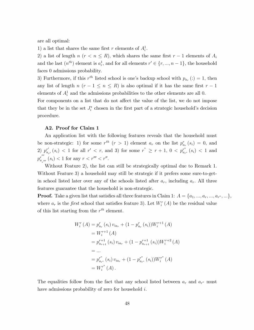
are all optimal:

1) a list that shares the same �rst r elements of A1i .

2) a list of length n (r < n � R); which shares the same �rst r � 1 elements of Aiand the last (nth) element is a1r; and for all elements r

0 2 fr; :::; n� 1g, the householdfaces 0 admissions probability.

3) Furthermore, if this rth listed school is one�s backup school with par (:) = 1; then

any list of length n (r � 1 � n � R) is also optimal if it has the same �rst r � 1elements of A1i and the admissions probabilities to the other elements are all 0.

For components on a list that do not a¤ect the value of the list, we do not impose

that they be in the set J�i chosen in the �rst part of a strategic household�s decision

procedure.

A2. Proof for Claim 1An application list with the following features reveals that the household must

be non-strategic: 1) for some rth (r > 1) element ar on the list prar (si) = 0, and

2) pr0ar0(si) < 1 for all r0 < r; and 3) for some r" � r + 1; 0 < pr"ar" (si) < 1 and

pr000

ar000 (si) < 1 for any r < r

000 < r00:

Without Feature 2), the list can still be strategically optimal due to Remark 1.

Without Feature 3) a household may still be strategic if it prefers some sure-to-get-

in school listed later over any of the schools listed after ar, including ar: All three

features guarantee that the household is non-strategic.

Proof. Take a given list that satis�es all three features in Claim 1: A = fa1; :::; ar; :::; ar"; :::g,where ar is the �rst school that satis�es feature 3): Let W r

i (A) be the residual value

of this list starting from the rth element.

W ri (A) = p

rar (si) viar + (1� p

rar (si))W

r+1i (A)

= W r+1i (A)

= pr+1ar+1(si) viar + (1� pr+1ar+1

(si))Wr+2i (A)

= :::

= pr"ar" (si) viar + (1� pr"ar"(si))W

r"i (A)

= W r"i (A) :

The equalities follow from the fact that any school listed between ar and ar" must

have admissions probability of zero for household i:

48

Consider an alternative (not necessarily optimal) application listB = fa1; :::; ar"; :::; ar"; :::g ;which di¤ers from A only in that it replace ar with ar": The residual value of this list

at its rth element (now ar") is given by

W ri (B) = p

rar"(si) viar" + (1� prar" (si))W

r+1i (B)

= prar" (si) viar" + (1� prar"(si))W

r+1i (A)

= prar" (si) viar" + (1� prar"(si))W

r"i (A)

> pr"ar" (si) viar" + (1� pr"ar"(si))W

r"i (A)

= W r"i (A)

The second and third line holds because the rest of list B is the same as A; and the

value of W k+1i (�) is independent of what one chooses in slot k; for any k > 1. The

third line follows because prar" (si) > pr"ar"(si) (admissions probabilities decrease over

rounds) and

viar" = Emax fuiar" ; �g > E (�) = 0:

Given that the �rst r� 1 elements are also unchanged, it is immediate that the valueof the whole list W 1

i (B) > W1i (A) :

B1. Detailed Functional FormsHousehold Characteristics: xi = [xi1; :::; xi5] ; where xi1 = I (edui < high school) ;

xi2 = I (edui = high school) ; xi3 = I (edui � College) ; xi4 = I (single parenti = 1) ;xi5 = sibling�s school (xi5 = 0 if outside school, 2 f1; :::Jg if non-private school, �9if no sibling).

School Characteristics: wj = [wj1; wj2; wj3; wj4], where wj1 is school quality, wj2 is

tuition level, wj3 is capacity, and wj4 = I (semi-public). Let qg (qb) be the 75th (25th)

percentile of school quality.

Home-school distance: dij; measured in 100 meters.

Zone Characteristics: Let Nz be the number of schools in zone z; and qz be the

average school quality in zone z:

B1.1 Utility functionsHousehold utility is given by uij = U (wj; xi; dij) + �ij: De�ne g (�) and C (�) such

49

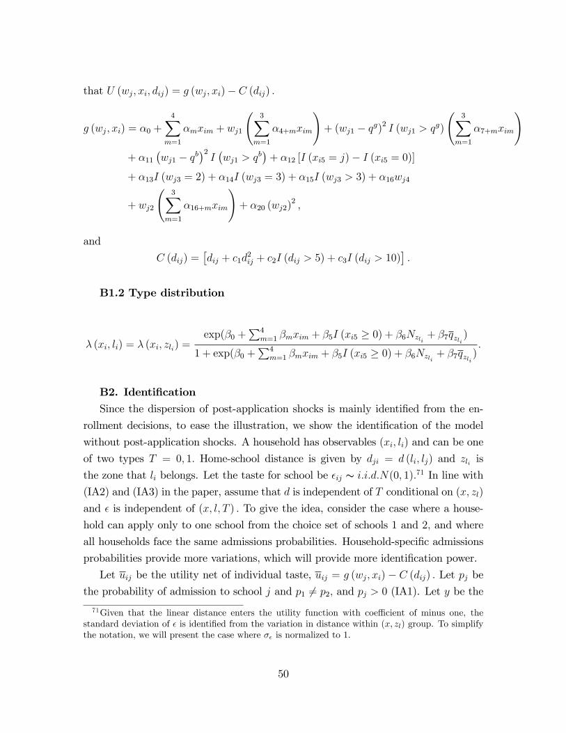
that U (wj; xi; dij) = g (wj; xi)� C (dij) :

g (wj; xi) = �0 +

4Xm=1

�mxim + wj1

3X

m=1

�4+mxim

!+ (wj1 � qg)2 I (wj1 > qg)

3X

m=1

�7+mxim

!+ �11

�wj1 � qb

�2I�wj1 > q

b�+ �12 [I (xi5 = j)� I (xi5 = 0)]

+ �13I (wj3 = 2) + �14I (wj3 = 3) + �15I (wj3 > 3) + �16wj4

+ wj2

3X

m=1

�16+mxim

!+ �20 (wj2)

2 ;

and

C (dij) =�dij + c1d

2ij + c2I (dij > 5) + c3I (dij > 10)

�:

B1.2 Type distribution

� (xi; li) = � (xi; zli) =exp(�0 +

P4m=1 �mxim + �5I (xi5 � 0) + �6Nzli + �7qzli )

1 + exp(�0 +P4

m=1 �mxim + �5I (xi5 � 0) + �6Nzli + �7qzli ):

B2. Identi�cationSince the dispersion of post-application shocks is mainly identi�ed from the en-

rollment decisions, to ease the illustration, we show the identi�cation of the model

without post-application shocks. A household has observables (xi; li) and can be one

of two types T = 0; 1: Home-school distance is given by dji = d (li; lj) and zli is

the zone that li belongs. Let the taste for school be �ij s i:i:d:N(0; 1):71 In line with(IA2) and (IA3) in the paper, assume that d is independent of T conditional on (x; zl)

and � is independent of (x; l; T ) : To give the idea, consider the case where a house-

hold can apply only to one school from the choice set of schools 1 and 2; and where

all households face the same admissions probabilities. Household-speci�c admissions

probabilities provide more variations, which will provide more identi�cation power.

Let uij be the utility net of individual taste, uij = g (wj; xi) � C (dij) : Let pj bethe probability of admission to school j and p1 6= p2; and pj > 0 (IA1). Let y be the71Given that the linear distance enters the utility function with coe¢ cient of minus one, the

standard deviation of � is identi�ed from the variation in distance within (x; zl) group. To simplifythe notation, we will present the case where �� is normalized to 1.

50

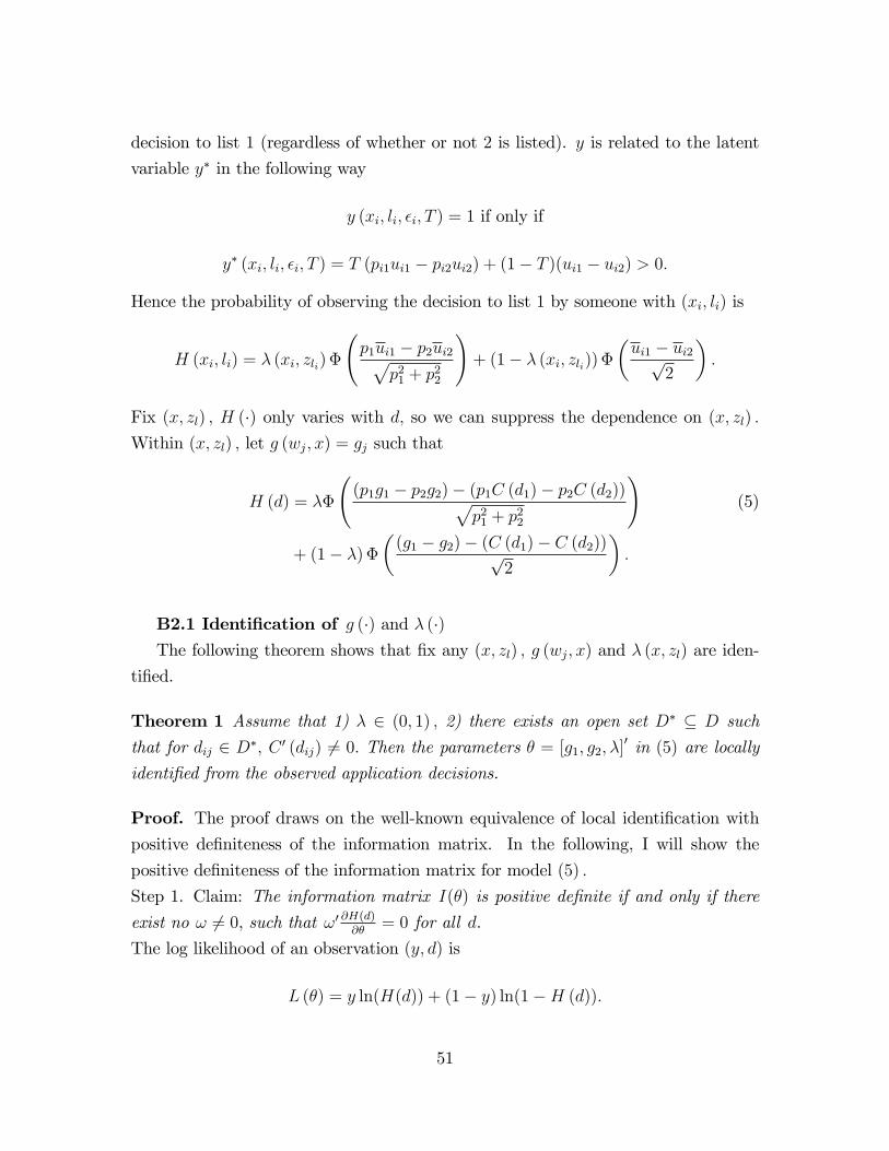
decision to list 1 (regardless of whether or not 2 is listed). y is related to the latent

variable y� in the following way

y (xi; li; �i; T ) = 1 if only if

y� (xi; li; �i; T ) = T (pi1ui1 � pi2ui2) + (1� T )(ui1 � ui2) > 0:

Hence the probability of observing the decision to list 1 by someone with (xi; li) is

H (xi; li) = � (xi; zli) �

p1ui1 � p2ui2p

p21 + p22

!+ (1� � (xi; zli)) �

�ui1 � ui2p

2

�:

Fix (x; zl) ; H (�) only varies with d; so we can suppress the dependence on (x; zl) :Within (x; zl) ; let g (wj; x) = gj such that

H (d) = ��

(p1g1 � p2g2)� (p1C (d1)� p2C (d2))p

p21 + p22

!(5)

+ (1� �) ��(g1 � g2)� (C (d1)� C (d2))p

2

�:

B2.1 Identi�cation of g (�) and � (�)The following theorem shows that �x any (x; zl) ; g (wj; x) and � (x; zl) are iden-

ti�ed.

Theorem 1 Assume that 1) � 2 (0; 1) ; 2) there exists an open set D� � D such

that for dij 2 D�; C 0 (dij) 6= 0: Then the parameters � = [g1; g2; �]0 in (5) are locallyidenti�ed from the observed application decisions.

Proof. The proof draws on the well-known equivalence of local identi�cation withpositive de�niteness of the information matrix. In the following, I will show the

positive de�niteness of the information matrix for model (5) :

Step 1. Claim: The information matrix I(�) is positive de�nite if and only if there

exist no ! 6= 0, such that !0 @H(d)@�

= 0 for all d.

The log likelihood of an observation (y; d) is

L (�) = y ln(H(d)) + (1� y) ln(1�H (d)):

51

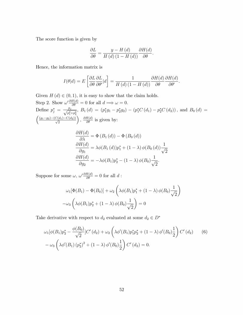
The score function is given by

@L

@�=

y �H (d)H (d) (1�H (d))

@H(d)

@�:

Hence, the information matrix is

I(�jd) = E�@L

@�

@L

@�0jd�=

1

H (d) (1�H (d))@H(d)

@�

@H(d)

@�0:

Given H (d) 2 (0; 1), it is easy to show that the claim holds.

Step 2. Show !0 @H(d)@�

= 0 for all d =) ! = 0:

De�ne p�j =pjpp21+p

22

; B1 (d) = (p�1g1 � p�2g2) � (p�1C (d1)� p�2C (d2)) ; and B0 (d) =�(g1�g2)�(C(d1)�C(d2))p

2

�; @H(d)

@�is given by:

@H(d)

@�= �(B1 (d))� � (B0 (d))

@H(d)

@g1= ��(B1 (d))p

�1 + (1� �)�(B0 (d))

1p2

@H(d)

@g2= ���(B1)p�2 � (1� �)�(B0)

1p2:

Suppose for some !; !0 @H(d)@�

= 0 for all d :

!1[�(B1)� �(B0)] + !2���(B1)p

�1 + (1� �)�(B0)

1p2

��!3

���(B1)p

�2 + (1� �)�(B0)

1p2

�= 0

Take derivative with respect to d2 evaluated at some d2 2 D�

!1[�(B1)p�2 �

�(B0)p2]C 0 (d2) + !2

���0(B1)p

�1p�2 + (1� �)�0(B0)

1

2

�C 0 (d2) (6)

� !3���0(B1) (p

�2)2 + (1� �)�0(B0)

1

2

�C 0 (d2) = 0:

52

De�ne (d) = �(B1)�(B0)

, divide (6) by �(B0) :

!1[ (d) p�2 �

1p2]� !2

��B1 (d) p

�1p�2 + (1� �)B0

1

2

�+!3

��B1 (d) (p

�2)2 + (1� �)B0

1

2

�= 0

(d) [!1p�2 � �B1p�2(!2p�1 � !3p�2)]� [

!1p2+ (!2 � !3) (1� �)B0

1

2] = 0 (7)

Since (d) is a nontrivial exponential function of d, (7) hold for all d 2 D� only if

both terms in brackets are zero for each d 2 D�, i.e.

!1p�2 � �B1 (d) p�2(!2p�1 � !3p�2) = 0 (8)

!1p2+ (!2 � !3) (1� �)B0 (d)

1

2= 0:

Take derivative of (8) again with respect to d2, evaluated at d2 2 D� :

��C 0 (d2) (p�2)2 (!2p

�1 � !3p�2) = 0

(!2 � !3) (1� �)C 0 (d2)1

2p2= 0:

Since � 2 (0; 1); pj > 0 (hence p�22 > 0) and C 0 (d2) 6= 0 for some d; we have

!2p�1 � !3p�2 = 0!2 � !3 = 0:

Given p1 6= p2 (hence p�1 6= p�2); follows that ! = 0:

B2.2 Identi�cation of C(dij):Given the identi�cation result from B2.1, and given that C(dij) is common across

(x; zl)�s; the parameters in C(dij) solves for the system of equations (5), where one

equation corresponds to one (x; zl) :

C. Priority Score StructureCase 1: Those who does not have a sibling in school have two levels: xia (xia+ b1)

for out-of-zone (in-zone) schools.

Case 2: Those whose sibling(s) is (are) in in-zone schools has 3 levels: xia (xia+ b1)

53

for out-of-zone (in-zone) non-sibling schools, and xia+ b1 + b2 for sibling schools.

Case 3: Those whose sibling(s) is (are) in out-of-zone schools has 3 levels: xia

(xia+ b1) for out-of-zone (in-zone) non-sibling schools, and xia+b2 for sibling schools.

Case 4: Those with sibling(s) in some in-zone school and sibling(s) in some out-of-

zone school has 4 levels: xia (xia+ b1) for out-of-zone (in-zone) non-sibling schools,

and xia+ b2 (xia+ b1 + b2) for out-of-zone (in-zone) sibling schools.

D. Additional Assumptions to Use the Data to its Full PotentialConsider an observed application list by household i

� eAi� of length n; in whichthe rth element is the �rst school that has admissions probability of 1 in the relevant

round�prj (si) = 1

�; and the tth element is the �rst leftover school listed (r � t) : We

impose the following structure.

A1. If i is strategic, then the schools listed after rth element are ranked, i.e., viar+1i>

::: > viani : However, we do not impose structure on how these schools are ranked with

respect to other schools, nor do we require that they belong to the candidate set J�i :

A2. If i is non-strategic, then the schools listed after the tth element are ranked, i.e.,

viat+1i> ::: > viani : By Condition (3) ; the schools listed after a

ti are ranked below any

schools listed before them, but we do not make assumptions on how they compare

with non-listed schools.

Notice that whether or not a household is strategic is probabilistic from the re-

searcher�s point of view. In our simulation, each household in the data will be repli-

cated by a large number of simulated households with identical observable character-

istics but di¤erent unobserved tastes for schools and di¤erent types.

E. The GS and TTC AlgorithmsE1. The GS algorithm assigns students as follows.

Round 1: Each school j tentatively assigns its seats to students who top-listed it, one

at a time following their priority order. If school j is over-demanded, lower-ranked

applicants are rejected.

In general, at Round r: Each school j considers the students it has been holding,

together with students who were rejected in the previous round but listed j as their

rth choice. Seats in school j are tentatively assigned to these students, one at a time

following their priority order. If school j is over-demanded, lower-ranked applicants

are rejected.

The algorithm terminates when no student is rejected and each student is assigned

54

her �nal tentative assignment.

The key di¤erences between GS and BM are 1) in each round, students are only

temporarily assigned to a school until the whole procedure ends; and 2) temporarily

held students are considered based only on priorities along with students who were

rejected from their choices in previous rounds and added into a school�s student

pool in the current round. As such, a previously held student can be crowded out

by a newly-added student who has higher priority. That is, top-listing a school

does not improve one�s chance of being �nally admitted to this school, which makes

truth-telling a (weakly) dominant strategy for households under GS. Moreover, GS

eliminates justi�ed envy. The appealing properties of GS, however, may con�ict with

Pareto e¢ ciency, as shown by Abdulkadiro¼glu and Sönmez (2003).

E2. The TTC algorithm assigns students as follows.

Round 1: Assign a counter for each school which keeps track of how many seats are

still available at the school, initially set to equal the school capacity. Each school

points to the student who has the highest priority for the school. Each student points

to her favorite school under her announced preferences.72 This will create ordered lists

of distinct schools (s) and distinct students (i) : (s1; i1; s2; i2; ::::), where s1 points at

i1; i1 points at s2; and s2 points at i2; etc. Because there are �nite number of schools,

at least one cycle will be formed, where ik (k � 1) points at s1: Although there maybe multiple cycles formed in a round, each school can be part of at most one cycle and

each student can be part of at most one cycle. Every student in a cycle is assigned a

seat at the school she points to and is removed. The counter of each school in a cycle

is reduced by one and if it reduces to zero, the school is also removed. Counters of

all schools that are not in any cycle stay put.

In general, at Round r: Each remaining school points to the student with highest

priority among the remaining students and each remaining student points to her

favorite school among the remaining schools. Every student in a cycle is assigned a

seat at the school that she points to and is removed. The counter of each school in a

cycle is reduced by one and if it reduces to zero the school is also removed. Counters

of all other schools stay put.

The algorithm terminates when all students are assigned a seat.

Intuitively, in each round TTC creates cycles of trade between individuals. Each

72A student announces her entire list of schools before the assignment starts. As such, the "point-ing" by a student is mechanically following her announced list.

55

individual in a cycle trades o¤ a seat in her highest-priority school for a seat in her

most preferred school among those that still have seats. Whenever such a cycle is

formed the allocation is �nal. Hence, the only way for an individual to improve her

allocation is through �stealing�another individual�s school assignment, which will in

turn make this other individual worse o¤. As such, TTC is Pareto e¢ cient as shown

by Abdulkadiro¼glu and Sönmez (2003), who also prove that TTC is truth-revealing.

However, TTC does not eliminate justi�ed envy because student-school priorities are

ignored in the TTC trade between individuals.

F. Policy Evaluation: The 2007 ReformThe 2007 reform gives priorities for households to access schools that are closest to

their home locations. Depending on households�home locations and strategic types,

the reform may have a¤ected them di¤erently. In order to assess these impacts, we

simulate the counterfactual outcomes for the 2007 applicants had they lived under

the 2006 regime, taking as given the 2006 admissions probabilities. The results gen-

erated from this experiment can be interpreted in two ways: 1) the results are at the

individual level, i.e., "what would have happened to a 2007 applicant had she applied

in 2006?"; 2) assuming that the 2006 and 2007 cohorts are two i.i.d. random samples

drawn from the same distribution, the results tell us "what would have happened to

all 2007 households if the reform had not happened and if they had played the same

equilibrium as the 2006 cohort?".

The �rst two columns of Table A10 present the fractions of winning and losing

households due to the 2007 reform. About 18% of households gained and 14% of

households lost from the reform. More non-strategic households were a¤ected, with

27% winners and 22% losers. Across educational groups, the high-school educated

group was the most likely to win (20%) and also the most likely to lose (15%) from the

reform. The last row shows the distribution within a particular group of households

who lived at the corner of school zones under the 2006 regime. In particular, we de�ne

corner households as those at least half of whose 2007 priority schools were not in

their pre-reform school zones. They accounted for over 15% of all 2007 households.

Not surprisingly, these households were more likely to be a¤ected by the reform

than an average household: 21% of them gained and 15% of them lost from the

reform. The last two columns of Table A9 show the changes in welfare, as measured

in utils and in welfare-equalizing fees. Overall, the gain from the 2007 reform was

worth a 23-euro decrease in school fees. The average welfare impacts were small for

56

strategic households, but much more signi�cant for non-strategic households. Across

educational groups, households with higher educated parents gained more.

G. Additional TablesG1. Model Fit

Table A1 Model Fit: Relevant List Length 2006 (%)

Edu < HS Edu = HS Edu �College Single Parents

Data Model Data Model Data Model Data Model

1 87.1 85.3 83.7 82.1 86.8 84.5 85.8 81.8

2 11.2 11.7 13.0 13.0 10.6 11.2 11.4 13.7

� 3 1.7 3.0 3.3 3.9 2.6 4.3 2.8 4.5

Table A2 Model Fit: Assignment Round 2006 (%)

Edu < HS Edu = HS Edu �College Single Parents

Data Model Data Model Data Model Data Model

1 93.2 95.1 92.0 93.7 93.7 94.1 94.0 93.4

2 2.7 1.7 3.5 2.3 2.3 2.6 1.9 2.7

� 3 1.6 0.1 1.5 0.5 1.3 0.2 1.4 0.2

Unassigned 2.5 3.1 3.0 3.5 2.7 3.1 2.7 3.7

Table A3 Model Fit: Top-Listed Schools 2006

Quality Distance (100m) Tuition (100 Euros)

Data Model Data Model Data Model

Parental Edu < HS 7.6 7.6 5.2 6.3 5.4 5.4

Parental Edu = HS 7.9 7.9 7.0 7.3 8.1 8.3

Parental Edu �College 8.2 8.1 8.7 8.3 9.9 10.0

Single-Parent 8.0 8.0 8.1 7.8 8.6 8.8

Table A4 Model Fit: Relevant List Length 2007 (%)

Edu < HS Edu = HS Edu �College Single Parents

Data Model Data Model Data Model Data Model

1 85.2 86.7 84.8 85.2 87.6 88.4 87.0 85.6

2 12.4 10.3 12.4 11.0 10.7 8.8 11.2 10.4

� 3 2.4 3.0 2.8 3.8 1.7 2.8 1.8 4.0

57

Table A5 Model Fit: Assignment Round 2007 (%)

Edu < HS Edu = HS Edu �College Single Parents

Data Model Data Model Data Model Data Model

1 91.0 94.8 90.6 94.3 93.7 95.0 91.3 94.4

2 3.7 1.7 3.2 2.3 2.2 1.7 2.9 2.0

� 3 1.6 0.2 2.2 0.2 1.6 0.7 1.4 0.5

Unassigned 3.5 3.3 4.0 3.5 2.5 2.6 3.3 3.1

Table A6 Model Fit: Top-Listed Schools 2007

Quality Distance (100m) Tuition (100 Euros)

Data Model Data Model Data Model

Parental Edu < HS 7.5 7.5 5.2 5.9 5.3 5.2

Parental Edu = HS 8.0 7.9 6.3 6.5 8.2 8.2

Parental Edu �College 8.2 8.1 7.8 8.0 9.7 9.9

Single-Parent 8.0 7.9 6.8 7.0 8.2 8.5

G2. Counterfactual Experiments

Table A7 Gains and Losses: BM to GS

Winner Loser

�utils �fees �utils �fees

Strategic 35.0 (44.9) -868.7 (774.5) -21.0 (20.3) 498.5 (577.5)

Non-strategic 43.2 (46.6) -987.1 (778.3) -26.0 (23.4) 567.7 (596.4)

Edu < HS 31.0 (39.0) -556.2 (559.9) -22.9 (21.8) 637.2 (574.0)

Edu = HS 38.4 (48.2) -937.2 (793.9) -21.7 (20.6) 496.7 (547.5)

Edu �College 35.1 (45.2) -1003.8 (816.0) -19.6 (19.2) 392.5 (589.3)

Table A8 Winners and Losers: BM to TTC

Winner Loser

�utils �fees �utils �fees

Strategic 30.5 (40.7) -802.7 (743.6) -25.5 (47.9) 409.2 (598.2)

Non-strategic 34.5 (43.1) -836.2 (747.1) -30.4 (61.1) 392.6 (583.1)

Edu < HS 27.4 (35.5) -513.2 (528.0) -21.3 (25.7) 551.0 (575.8)

Edu = HS 33.0 (43.6) -873.7 (763.5) -28.8 (47.4) 432.4 (582.9)

Edu �College 30.9 (41.4) -954.2 (799.5) -25.8 (59.9) 289.1 (601.5)

58

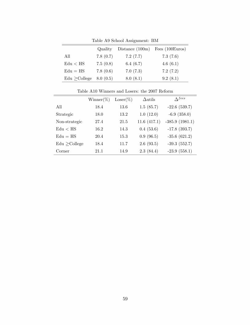
Table A9 School Assignment: BM

Quality Distance (100m) Fees (100Euros)

All 7.8 (0.7) 7.2 (7.7) 7.3 (7.6)

Edu < HS 7.5 (0.8) 6.4 (6.7) 4.6 (6.1)

Edu = HS 7.8 (0.6) 7.0 (7.3) 7.2 (7.2)

Edu �College 8.0 (0.5) 8.0 (8.1) 9.2 (8.1)

Table A10 Winners and Losers: the 2007 Reform

Winner(%) Loser(%) �utils �fees

All 18.4 13.6 1.5 (85.7) -22.6 (539.7)

Strategic 18.0 13.2 1.0 (12.0) -6.9 (358.0)

Non-strategic 27.4 21.5 11.6 (417.1) -385.9 (1981.1)

Edu < HS 16.2 14.3 0.4 (53.6) -17.8 (393.7)

Edu = HS 20.4 15.3 0.9 (96.5) -35.6 (621.2)

Edu �College 18.4 11.7 2.6 (93.5) -39.3 (552.7)

Corner 21.1 14.9 2.3 (84.4) -23.9 (558.1)

59