Structural VAR and Finance

AbstractIn this paper, I discuss VAR (vector autoregression) framework, which is widely used in finance and economics to examine dynamic relations among variables. I also discuss the identification of VAR model (structural VAR) using several examples from finance.

Bong Soo Lee

1

I. Introduction/Motivations - Dynamic effects in a multivariate system• The effect of financial news on stock prices (or

returns) [r, y, , d, c P (or sr)] ex. Chen, Roll, Ross (JB, 1986)

• Analysis of policy effects (Ms, G) on stock market

- Relative importance APT (DY, TP, , IPG, Ms, TOT, EX RATE, oil price,

…)CECF (NAV or USMR) Second board market returns (e.g., NASDAQ,

KOSPI, KOSDAQ)

2

- Empirical tool: VAR

(vector autoregression) framework

- Identification issue: under-identified VAR

• Cholesky identification: Ordering issue• Permanent/temporary shocks (components), • substitution/complement shocks,• positive/negative shocks.

- The role of theory3

II. VAR (vector autoregression) framework

1. Dynamic effects (impulse responses)

a. VAR (vector autoregressive representation)

4

1where ( ) ( ) , , var( ) .1

1 1 11

( ) 1

1

nt t n

X A(s)X e A(L)X et t s t tt 1s 1(m 1)

sA L A s L L X X ets

X eX t tt

X eX A L ititit ij

eXX mtmt mt

X

jt-s

( )1 1

( ): the effect of X on (in s periods) ?

coeff: ( ) [ ( )],

but X is serially and contemporaneously correlated.

mA s X eit ij jt s its j

A s Xij jt s itA s A sij

5

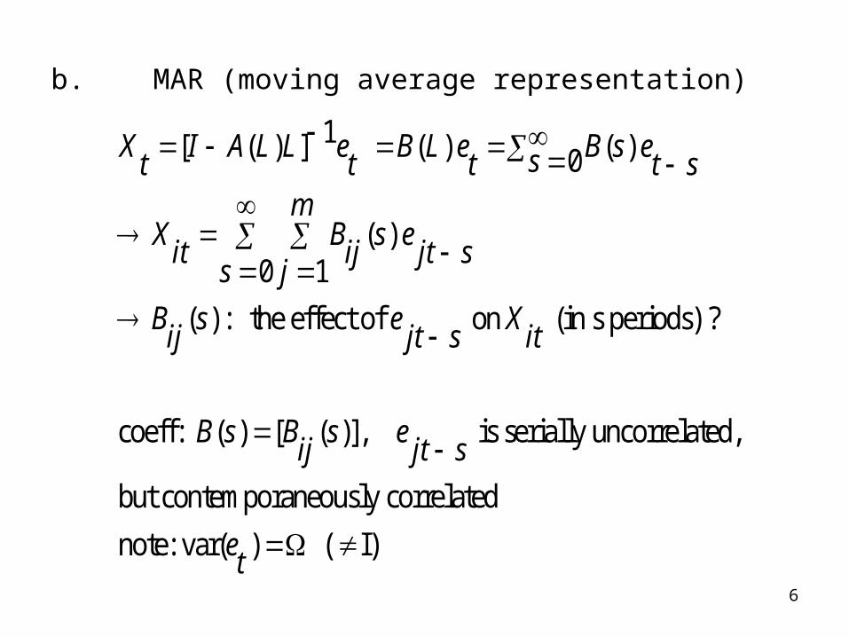
b. MAR (moving average representation)

1[ ( ) ] ( ) ( )0

( )0 1

( ) : the effect of on (in s periods) ?

coeff: ( ) [ ( )], is serially uncorrelated,

but contemporaneously cor

X I A L L e B L e B s est t t t sm

X B s eit ij jt s

s j

B s e Xij jt s it

B s B s eij jt s

related

note: var( ) ( I)et

6

C. Orthonormalized MAR

-1 .

var( ) (positive definite matrix)

' , where G is a lower-triangular matrixt

Definee

G G

1( ) ( ) ( )

( ) ( ) ,

1where ( ) ( ) , and ut-1 1and var( ) var( ) ' G(G ' ) ' .

Now, ( ) ( ) X ( )it 0 1

( ) the

t

t

X B L e B s e B s G Get t s t ss sc s u C L ut ssc s B s G Getu Ge G G G G It t

mX C L u c s u c s ut t t s ij jt ss s j

c sij

.

effect of on X . (or responses to shocks it

(or innovations) to particular variables).

coeff: c( ) [ ( )] : serially & contemporaneously uncorrelated

u jt s

s c sij

7

- Examples:

• The effect of financial news on stock prices (or returns)

[r, y, , d, c P (or sr)],

ex. Chen, Roll, Ross (JB, 1986)

• Analysis of policy effects (Ms, G) on stock market

• Stylized facts (dynamic relation)

• Transmission mechanism (ex. Volatility, …)8

2. Forecast error decompositions --- relative importance.( ) , with var ) .

( )0 1

[ | , 0] ( ) .1

t-step ahead forecast error Zit1

[ | , 0] ( )0 1

t-step ahead forecast error var

X C L u (u It t tm

X c s uit ij jt ss jm

E X X s c s usit ij jt ss t j

t mX E X X s c s usit it ij jt ss j

iance of

1 22 ( ) ( )0 1

because ( ) 0 for i j , ( ) 0 for t s , and

2 ( ) 1.

t-step ahead forecast error variance of

Xit m

E Z c sit ijs jE u u E u uit jt jt js

E u u ujt jtX accounted fori

by i

12

01

2

0 1

( )

( )

t

ijst m

ijs j

c snnovations in X j

c s

9

- Applications• relative importance• exogeneity of (policy) variables• causal relations

- examples:• APT (DY, TP, , IPG, Ms, TOT, EX RATE, oil price,

…)• CECF (NAV or USMR) [Lee and Hong (JIMF, 2002)]• Second board market returns (e.g., NASDAQ, KOSPI,

KOSDAQ) [Lee, Rui, and Wang (JFR, 2003)]

10

3. Identification:

Under-identified system of VAR

Note: Dynamic effects and relative importance

are based on the orthonormalized MAR

coefficients C(L).

VAR (data): ( ) ; var(e )1 t

MAR (theory): ( ) ; var(u )t

X A L X et t tX C L u It t

11

Question: Given estimates of A(L) and , how to identify C(L)?

Clue (match):

(i) 01 1(ii) C [ ( ) ] [ ( ) ] 0

1( ) [ ( ) ] 0[i.e., C( ) can be identified once c is found]0

again, (i) '0 0 01 -1[Re ' (i.e., G c )]0

e c ut t

(L)u I A L L e I A L L c ut t t

C L I A L L c

L

e c u c ct t

call G G

12

0 0

0 0 0 011 11 12 11 21

0 0 0 021 22 21 22 12 22

0

(1) Bivariate case (m 2): '

. c c c c

c c c c

3 restrictions (eqns) with 4 unknowns (elements of c )

We need at least on

c c

0

0 0 0 0 0 011 12 13 11 21 31110 0 0 0 0 0

21 22 21 22 23 12 22 320 0 0 0 0 0

31 32 33 31 32 33 13 23 33

e additional restrction on c [from theory].

(2) Trivariate case (m 3)

c c c c c c. . . c c c c c c

c c c c c c

0

0

6 restrictions (eqns) with 9 unknowns (elements of c )

We need at least three additional restrction on c [from theory].

13

Identification 1. Cholesky decomposition

0 0111 0 i.e., 0

0 120 021 22

cc G c

c c

0connrestrictioadditional

Cholesky decomposition imposes a certain ordering c120 = 0

[2nd variable does not affect the first variable contemporaneously]1. u2 has no contemporaneous effect on X1.

2. Place an exogenous variable first [e.g., policy variable (Ms, G,…)]

14

Note : trivariate case

• in general, the ordering of variables in VAR matters

0 0 011

1 0 0 0 0 0 0 i.e., 0.0 21 22 12 13 23

0 0 031 32 33

c

c G c c c c c

c c c

0cadditional restriction on

15

Identification 2. Permanent/temporary restriction

[Blanchard & Quah (1989)]

12 1 12 1 12 120 0

11 11 12

22 21 22

1 1 11 1 12 2

( ) | ( ) | ( ) (1) 0.

( ) ( ) Let ( )

( ) ( )

(1 ) ( ) ( )

[

sL L

s s

ttt t

tt

t t t t

c L c s L c s c

uX c L c LX c L u

uX c L c L

X L X c L u c L u

c

* *11 11 1 12 12 2

12

* *111t 11 1 12 2

12 2 1

2

(1) (1 ) ( )] [ (1) (1 ) ( )]

with (1) 0(1)

X [ ( )] ( )1

(1) 0 implies that the cumulative effect of u on X is zero

[or u has only a t

t t

t t

L c L u c L c L u

cc

c L u c L uL

c

1

1

1t

2t

emporary (transitory) effect on X ]

But u has a permament effect

u a permanent shock [

u a temporary shock

16

- Applications: • Permanent earnings hypothesis of dividend

[ Lee (RFS, 1996)].• Stock market responds more strongly to

permanent earnings [Lee (JFQA, 1995)].• Permanent, temporary, and non-fundamental

components of stock prices [Lee (JFQA, 1998)].• Stock returns and inflation [Hess and Lee (RFS,

1999)]• Payout policy (Flexibility Hypothesis): Dividends

are related to permanent earnings, and share repurchases are related to transitory earnings [Lee and Rui (JFQA, 2007)]. 17

12

10

1 0 011 1211 120 0

21 22 21 22

22 12

Note: How to implement the restriction (1) 0?

from C( ) [ ( ) ]

I-A ( ) ( )

( ) 1 ( )

I-A ( ) (1 =

c

L I A L L c

c cL L A L LA L L A L L c c

L L A

0 011 120 0

21 11 21 22

0 012 12 22 22 12

^ ^0 0

12 12 1 12 22 22 12

)( ) 1 ( )

. .det min .

. .

1 So ( ) { [1 ( ) ] ( ) }

(1) ( ) | [1 (1)] (1) 0.

Thus, giv

L

c cL LA L L A L L c c

where er ant of

c L c A L L c A L L

c c L c A c A

^ ^0

12 22 120

en estimates of (1) and (1), c (1) 0 provides a restriction on c .

c

A A

additional restriction on

18

t

1 2

t

t

11 121

Let earni ngs, X , be ( ) ( ) , var( ) .

1

Let , the spread, be

X [i.e., ~ (1,1)].

D

Consider

( ) ( )

st t t tt t

t

t t t

tt tt

t tt

q LX X X e r L e where e IL

s

s X D CI

c L c LD DDZ

X Ds

1

221 22.

( ) ( )t

t

eec L c L

Application 2.1 Dynamic dividend behavior [Lee (RFS, 1996)]

19

Model 1. Dividends are proportional to the permanent component of earnings:

Characterized by the restriction that

C12(L) = C21(L) = 0.

Implications: • Temporary changes in earnings do not affect

dividend (changes).• Permanent changes in earnings do not affect the

spread.

pt tD X

20

Model 2. Dividends are proportional to a present discounted value of future expected earnings:

(1) 012

the transitory change in earnings does not have a long-term effect on divideds

the PAH:* [ ], (0,1)1

*Model 3. ( ) 012 dividends are

kD E X ct t t kk

D b D D bt t t

pD X c Lt t

*12 22

22

not affected by transitory changes in earnings .*Model 4. (1) 012

Model 5. (1) & (1) 0

Model 5 is characterized by (1) 0.t t

kD E X ct t t kkD X c c

c

21

• Earnings and dividends respond proportionately to transitory changes in earnings so their net effect on the spread is zero.

• This requires dividends to respond to the transitory changes in earnings.

• Against the permanent earnings hypothesis (PEH).

22

Application 2.2 Permanent & temporary components in stock prices [Lee (JFQA, 1995)]

Proposition: The stock price valuation model (PV model) is characterized by the restriction c12(1)=0 on the following bivariate model:

( ) ( )1 111 12( ) ( )

21 22 21

p pp ec L c Lt tt tZt s c L c L ep dt tt t

23

1 .

1 11 1

j jp E d d E dt t t j t t t j

j j

- Comparison w/ Fama & French (1988).

(i) F/F assume that log stock price is the sum of r.w. and an AR(1) process. Lee (1995) does not restrict the permanent component to be a r.w. and the temporary component to be an AR (1) process. The data determines the two components.

(ii) In F/F, price is not related to dividends.In Lee, price components are due to dividend components, and they are related by the stock price valuation model.

(iii) F/F model predicts ARMA (1,1) model of stock returns.

US data implies ARMA (2,2) model.

1 1 2 2( ) (1 ) ( ) .p st t t t tp p p g L e L g L e

24

Application 2.3 Permanent, temporary, and non-fundamental components of stock prices: Lee (JFQA, 1998) - Use log-linear models

• Model.

11 2 2

1

t2 1

: log earnings.( )

( )1

: log dividends.

Case 1: with time-constant interest rate

Case 2: with

p st t t

t t

jt t t t jt j

jt t t jt t j

y y yq L

e q L eL

s d y E y

s p d E d

t2 1 t j

2 1 t j t j

time-varying interest rates

[ -r ]

Case 3: with time-varying expected excess stock returns

[ -r - ]

jt t t jt t j

jt t t jt t j

s p d E d

s p d E d

25

Proposition 1. Models of earnings, dividends, and prices in case 1 are characterized by the restrictions

12 13 23

11 12 13 1

1 21 22 23 2

2 31 32 33 3

1t

(1) 0, ( ) 0, and ( ) 0,

( ) ( ) ( )

on ( ) ( ) ( ) ,

( ) ( ) ( )

where

e permanent fundamental innov

t t

t t t

t t

c c L c L

y c L c L c L e

Z s c L c L c L e

s c L c L c L e

2t

3t

ation

e temporary fundamental innovation

e non fundamental innovation.

26

• Proposition 2. Models in case 2 are characterized by the restrictions

12 13 23

11 12 13

21 22 23

2 31 32 33

t

dt

( ) 0, ( ) 0, and ( ) 0,

( ) ( ) ( )

on ( ) ( ) ( ) ,

( ) ( ) ( )

where

dr

e divid

t dt

t t rt

t nt

t t

c L c L c L

d c L c L c L e

Z dr c L c L c L e

s c L c L c L e

d r

rt

nt

end innovation

e interest rate innovation.

e non fundamental innovation.

27

Proposition 3 . Models in case 3 are characterized by the restrictions12 13 14 23 24 34

11 12 13 14

1 21 22 23 24

31 32 33 34

2 41 42 43 44

(1) 0, ( ) 0, ( ) 0, ( ) 0, ( ) 0, ( ) 0,

( ) ( ) ( ) ( )

( ) ( ) ( ) ( )on

( ) ( ) ( ) ( )

( ) ( ) ( ) (

t

tt

t

t

c c L c L c L c L and c L

c L c L c L c Lys c L c L c L c L

Zdr c L c L c L c Ls c L c L c L c

1

2

11 12 13 14 1

21 22 23 241

31 32 33 34

2 41 42 43 44

,

)

or

( ) ( ) ( ) ( )

( ) ( ) ( ) ( )on

( ) ( ) ( ) ( )

( ) ( ) ( ) ( )

t

t

rt

nt

tt

tt

t

t

eeeeL

c L c L c L c L eyc L c L c L c Ls e

Zc L c L c L c L

s c L c L c L c L

2

t t

1t 2t

rt

,

where the log excess stock return over short debt interest r . e ,e permanent and temporary fundamental innovation

e ,e

t

t

nt

t t t

ee

dr d r

t

nt

interest rate and excess return innovation e non fundamental innovation.

28

Application 2.4 Stock returns and inflation with supply and demand disturbances: Hess and Lee (1999, RFS)

• Theoretical model is characterized by the restriction

12

11 12

21 22

tst

(1) 0

( ) ( ),

( ) ( )

where the log of stock price. stock return. inflation rate. supply shock.

stt

t dt t

t

t

C on

C L C LspZ

C L C L

spsp

demand shock.dt

29

- Motivation and observation:

srt and t are negatively correlated in post-war period, but positively correlated in pre-war period.

- Findings and our results:• Supply components of srt and t are negatively

correlated, whereas demand components are positively correlated.

• Supply component (shock)------permanent• Demand component (shock)------temporary• Supply shock is more important in post-war

period, but demand shock is more important in pre-war period.

30

Application 2.5 Flexibility Hypothesis (Temporary Cash Flow):

- Lee and Rui (JFQA, 2007) Dividends: ongoing commitment, to distribute permanent cash flows,

Share repurchases: to pay out temporary cash flows, thus preserve

financial flexibility relative to dividends - Jagannathan et al. (2000), Guay and Harford (2000), Lie (2000) et al.

(2000)

• = permanent shock and = temporary (or stationary) shock.

t t t t

11 12

21 22

Z1 = [ Y , (RP/Y) ]' = C(L) , or

( ) ( ) ,

( / ) ( ) ( )

pt t

Tt t

Y C L C L

RP Y C L C L

2 [ ,( / ) ]' ( )t t t tZ Y D Y C L

11 12

21 22

( ) ( ).

( / ) ( ) ( )

pt t

Tt t

Y C L C L

D Y C L C L

Ptε T

tε31

- Identification: .• H0: RP are not related to the permanent component of

earnings, .• H0: RP are not related to the temporary component of

earnings, .

• H0: Div are not related to the permanent component of earnings, .

• H0: Div are not related to the temporary component of earnings, .

21( ) 0C L

22( ) 0C L

21( ) 0C L

22( ) 0C L

32

Identification 3. Substitutes and complements

• zt = [X1t, X2t]' = C(L) t, or 1

11 12

221 22

1 ( ) ( ) ,

2 ( ) ( )t t

t t

X C L C L

X C L C L

restriction on the substitution disturbance, ts :

the coefficients in C12(L) and C22(L) add up to zero:

k c12k + k c22

k = C12(L)|L=1 + C22(L)|L=1 = C12(1) + C22(1) = 0, where Cij(L)|L=1 = Cij(1) = k cij

k represents the cumulative effect of the j-th disturbance on the i-th variable over time.

0connrestrictioadditional

Examples: •payout policy: dividends versus share repurchases•stocks and bonds: correlations vary•Banking sector versus stock market in economic development 33

Application 3.1 The Substitution Hypothesis : Lee and Rui (JFQA, 2007)

• Grullon and Michaely (2002): corporations have been substituting share repurchases for dividends.

• Jagannathan et al. (2000): repurchases seem to serve the complementary role of paying out short-term cash flows and not appear to be replacing dividends.

• the following bivariate moving average representation (BMAR):

,

= the complement shock, = the substitution shock;

• Identification of Substitution and Complement Effects

ct

11 12

21 22

( / ) ( ) ( ) ,

( / ) ( ) ( )

ct t

st t

D Y C L C L

RP Y C L C L

[( / ) ,( / ) ]' ( )t t t tZ D Y RP Y C L

12 22 12 1 22 1 12 22( ) | ( ) | (1) (1) 0k kL Lk k

c c C L C L C C

ct

34

Application 3.2 Correlation Coefficients between Stock and Bond Returns

Table 1. Correlation Coefficients between Stock and Bond Returns

Panel A. Based on Monthly Real Returns

Period Canada Germany Japan U.K. U.S. 86-99 23.94%*** 23.61%*** 10.68% 39.36% *** 25.67%*** 00-07 -6.13% -45.31%*** -30.95%***-20.39%** -35.90%*** 86-07 15.91%*** 1.44% 4.90% 27.12%*** 4.00%

Q: How to understand different corr. across countries and over time? (Hong, Kim, & Lee (2009, WP))

35

zt = [Rt, Qt]' = C(L) t, or

where Rt = stock return; Qt = bond returns;

t is a 2 x 1 vector consisting of ty and t

s ;

ty = income effect shock; t

s = substitution effect shock

• Identifying restriction:

11 12

21 22

( ) ( )

( ) ( )

yt t

st t

R C L C L

Q C L C L

12 22 12 1 22 1 12 22( ) | ( ) | (1) (1) 0k kL Lk k

c c C L C L C C

36

Identification 4. Positive and negative shocks / components

zt = [X1t, X2t]' = C(L) t, or

Restrictions: c11

0 + c120 = 0

• Examples: 1. stock returns and volatility

2. stock returns and inflation: to identify two sources of shocks: Lee (2009, JBF)

111 12

221 22

1 ( ) ( ),

2 ( ) ( )t t

t t

X C L C L

X C L C L

37

•

Application 4.1 Stock returns and volatility

38

•

39

•

Application 4.2 Stock returns and inflation

40

41

- Observation:• Between stock returns and inflation, we observe + and -

correlation in pre-war and post-war period, respectively.- Interpretation:

• both +/- shocks to inflation have positive effect on SR.• AD shock drives a + correlation between inflation and

SR, while AS shock drives a – correlation;• + inflation shock that reflects AD is more important in

pre-war period, and - inflation shock that reflects AS is more important in post-war period.

• we observe + correlation between stock returns and inflation in pre-war period, and – correlation in post-war period.

• Not easily compatible with ‘the inflation (money) illusion hypothesis’ that anticipates only negative correlation.

42

III. Concluding Remarks

-VAR: dynamic effects & relative importance

-VAR: under-identified

-To achieve identification:

introduce restrictions from theory and test implications (hypotheses)

-Examples(i)permanent/temporary

(ii)Substitutes/complements

(iii)Positive/negative

43