structure of entropy solutions to the eikonal equation

Digital Object Identifier (DOI) 10.1007/s10097-002-0048-7

J. Eur. Math. Soc. 5, 107–145 (2003)

Camillo De Lellis · Felix Otto

Structure of entropy solutions to the eikonal equation

Received June 24, 2002 / final version received November 12, 2002Published online February 7, 2003 – c© Springer-Verlag & EMS 2003

Abstract. In this paper, we establish rectifiability of the jump set of an S1–valued con-servation law in two space–dimensions. This conservation law is a reformulation of theeikonal equation and is motivated by the singular limit of a class of variational problems.The only assumption on the weak solutions is that the entropy productions are (signed)Radon measures, an assumption which is justified by the variational origin. The methodsare a combination of Geometric Measure Theory and elementary geometric arguments usedto classify blow–ups.

The merit of our approach is that we obtain the structure as if the solutions werein BV, without using the BV–control, which is not available in these variationally motivatedproblems.

Key words. entropy solutions – partial regularity – singular perturbation – conservationlaws – rectifiability

1. Introduction

1.1. Motivation

Consider an energy functional of the form

Fε(mε) =∫

�

(ε |∇mε|2 + 1

ε

(1 − |mε|2

)2)+ 1

ε

∫R2

∣∣∇−1(∇ · mε)∣∣2 (1)

defined on the space of vector fields m : � → R2. Here∫

R2

∣∣∇−1(∇ · mε)∣∣2 =∫

R2|∇u|2 where − �u = ∇ · mε.

In this paper, we study the regularity of elements m of the “asymptotic admissibleset”. By the asymptotic admissible set of a sequence of functionals {Fε}ε↓0, we

C. De Lellis: Max–Planck Institute for Mathematics in the Sciences, Inselstr. 22–26, 04103Leipzig, Germany, e-mail: [email protected]

F. Otto: Institut für Angewandte Mathematik, University of Bonn, Wegelerstr. 10, 53115Bonn, Germany, e-mail: [email protected]

Mathematics Subject Classification (2000): 49N60, 35D10, 35L65, 35L67

108 Camillo De Lellis, Felix Otto

understand the set of all strong limits m (say, in L p(�) for all p < ∞) of sequences{mεn}n↑∞ which are bounded in energy.

What can we expect? In view of the 1ε–terms in (1), such a limit m satisfies

|m|2 = 1 a.e. and ∇ · m = 0 distributionally. (2)

There are two ways of looking upon (2) which are particular to two space dimen-sions. The first point of view is: since ∇ · m = 0, there exists a stream function ψ

such that m can be written as its gradient rotated by π2 , that is, ⊥∇ψ = m. Then

the first condition of (2) turns into the eikonal equation

|∇ψ|2 = 1 a.e. . (3)

The second point of view is: since |m|2 = 1, we may introduce a phase θ such thatm can be written as (m1, m2) = (cos θ, sin θ). Then the second condition of (2)turns into a scalar conservation law

∂ cos θ

∂x1+ ∂ sin θ

∂x2= 0 distributionally. (4)

Both (3) and (4) are rigid for smooth ψ resp. θ , as can be seen from the charac-teristics of these first order equations. But they practically lose all this rigidity ifψ is only Lipschitz or θ is only an essentially bounded function. The concept ofviscosity solution resp. of entropy solution restores the “right amount” of rigidity.But these concepts seem a priori unrelated to our variational problem.

Which properties beyond (2) can be expected? In view of the ε in front ofthe Dirichlet integral, finite–energy limits m will not be smooth in general. Aswe shall presently see, the scaling of the energy Fε is just such that it “sees”one–dimensional discontinuities (jumps) of the limit m. In view of (2), the normalcomponent of m is continuous across jumps. The line–energy density associatedwith jumps of m can be inferred from the one–dimensional version of (1), the localvariational problem

Fε(mε) :=∫ (

ε

∣∣∣∣dmε

dx1

∣∣∣∣2

+ 1

ε

(1 − |mε|2

)2 + 1

ε(mε,1 − m0,1)

2

)dx1 . (5)

Here m0,1 corresponds to the (prescribed) normal component of m. Rescalinglength as x1 = ε x1, one sees that the line–energy density is indeed O(1) in ε. Moreprecisely, a standard calculation shows that for m±

0 ∈ S1 with m±0,1 = m0,1,

min{

Fε(mε) | mε → m±0 as x1 → ±∞

}= O(∣∣m+

0 − m−0

∣∣3). (6)

The fact that the line–energy density is O(1) in ε naively suggests that a finite–energy limit m has a moderately regular one–dimensional discontinuity set. Thecubic degeneracy O(|m+

0 − m−0 |3) in the jump size |m+

0 − m−0 | on the other hand

indicates that we possibly do not control the total variation of m (more discussionon this in Subsect. 1.4). In the main result of this paper, Theorem 1, we willnevertheless establish regularity properties for m as if it were of bounded variation.

Structure of entropy solutions to the eikonal equation 109

1.2. Statement of result

The point of view (4) suggests to borrow the concept of entropies from conservationlaws to further characterize the asymptotic admissible set. Following [13], weintroduce

Definition 1. A smooth and compactly supported function � : R2 → R2 will becalled an entropy if for every open set � and every smooth m : � → R2 we have(∇ · m = 0 and |m|2 = 1

) ⇒ ∇ · [�(m)] = 0.

A particular set of entropies has first been introduced by Jin and Kohn as“calibrations” to establish lower bounds on the energy which are optimal in thelimit ε ↓ 0 [19]. Later, the concept of entropies, together with other tools fromconservation laws such as the div–curl–Lemma and Young measures, has beenused to establish

{Fε(mε)}ε↓0 bounded ⇒ {mε}ε↓0 ⊂ L p precompact,

see [2], [13], [26]. An important ingredient was the estimate∣∣∫∇ · [�(mε)]ζ

∣∣ ≤ C�

(Fε(mε) sup |ζ | + (ε Fε(mε)

∫ |∇ζ |2)1/2)

(7)

for an arbitrary entropy � and test function ζ . As a variation of Definition 1.3in [2], this motivates the following:

Definition 2. We call A(�) the set of essentially bounded m : � → R2 with (2)

and such that for every entropy �,

µ� := ∇ · [�(m)] is a measure of locally finite total variation.

We call the µ�’s entropy measures.

In view of (7), the asymptotic admissible set is a subset of A(�). Our mainresult is on the structure of m ∈ A(�):

Theorem 1. For m ∈ A(�) there exists J ⊂ � such that

(a) J isH1 σ–finite and rectifiable;(b) forH1–a.e. x ∈ J,

limr↓0

1

r2

∫Br(x)

|m(y) − mx,r | dy = 0,

where mx,r is the average of m on Br(x);(c) forH1–a.e. x ∈ J, there exist m+(x), m−(x) ∈ S1 with

limr↓0

1

r2

{∫B+

r (x)|m(y) − m+(x)| dy +

∫B−

r (x)|m(y) − m−(x)| dy

}= 0,

where B±r (x) := {y ∈ Br(x)| ± y · η(x) > 0} and η(x) is a unit vector normal

to J in x;


(d) for every entropy �

µ� J = [η · (�(m+) − �(m−))]H1 J, (8)

µ� K = 0 for any K ⊂ � \ J with H1(K ) < ∞. (9)

This is somewhat less than what we would get for free if m had bounded totalvariation using the fine properties of BV functions and the Vol’pert Chain Rule (seeSect. 3.7 and Theorem 3.96 of [3]). Despite the fact that we cannot expect boundedtotal variation, we conjecture that m has the same structure. Hence we expect thatpoints (b) and (d) can be improved to

Conjecture 1.

(b’) forH1–a.e. x ∈ J , x is a Lebesgue point of m.(d’) µ� = [η · (�(m+) − �(m−))]H1 J for every entropy �.

1.3. Mathematical context

Why are we interested in (1)? Because its asymptotic admissible set contains theasymptotic admissible sets for two other problems which have been intensivelystudied in the past years:

Problem 1. The functionals

F1ε (mε) =

∫�

(ε |∇mε|2 + 1

ε

(1 − |mε|2

)2)(10)

on the set of vector fields satisfying ∇ · mε = 0.

Problem 2. The functionals

F2ε (mε) =

∫�

ε |∇mε|2 + 1

ε

∫R2

∣∣∇−1(∇ · mε)∣∣2 (11)

on the set of vector fields satisfying |mε|2 = 1.

Problem 1 was first considered by Aviles and Giga [6]. It was later proposed byGioia and Ortiz [24] as a model for delamination of compressed thin elastic films(“blisters”), where the stream function ψ is the height of the delamination (for moreon modeling of thin–film blistering phenomena see [8]). Since then, many partialresults on the asymptotic admissible set and the limiting variational problem (the�–limit) have been obtained: [6], [7], [2], [19], [13], [18], [17], [10].

Problem 2 was introduced by Rivière and Serfaty [26] in the context of thinferromagnetic films. Here m is the magnetization; see for instance [12] for thin–film models in ferromagnetism. The results for Problem 2 are stronger than forProblem 1 (see [26], [25], [21], [5] and [4]). This might be related to the fact thatthere are no vortices on the ε–level, which leads to a tighter control of the asymp-totic admissibility set. Since vortices play an important role in micromagnetics,Alouges, Rivière and Serfaty [1] have introduced a slight variation of (1) (where


the penalization of |m|2 − 1 is stronger than the one of ∇ · m) which allows forvortices on the ε–level — and therefore has more the character of Problem 1.

One might wonder whether we give up too much information by replacingthe asymptotic admissible set of Problem 1 or 2 by A(�). Indeed, it can be seenfrom making C� in (7) more explicit that the measures µ� enjoy a weak formof uniform control in �. The kinetic formulations (see [18] and [25]) quantifythis uniform control. But this uniform control differs from problem to problemand would not substantially simplify our proof. This is why we stick to the moreflexible A(�).

Parallel to but independently from us, Ambrosio, Kirchheim, Lecumberry andRivière [4] have proved the same result for a set A(�) which contains the asymptoticadmissible set of Problem 2. A(�) is potentially different from A(�): next to (2),its definition is based on a phase θ , see (4). Their class of entropies � are functionsof the phase θ , and not just of m — which is appropriate for Problem 2. Asa particular consequence, ∇ · [�(m)] = 0 for their entropies if m is a vortexm(x) = (−x2, x1)/|x|, whereas our entropies are oblivious to a vortex — asthey should be for Problem 1. In this sense, our entropies yield less control thantheir entropies. This is reflected in the fact that our class of possible blow–ups isa priori richer than theirs, so that we need more arguments to rule most of themout. The proof of [4] is shorter and uses different methods, in particular based ona comparison among certain maps in A(�) and viscosity solutions of the eikonalequation (see [5]).

1.4. Outlook

One might wonder what the difficulties in this problem are. In our opinion thedifficulties come from the fact that the asymptotic admissible sets for Problem 1and 2, and a fortiori A(�), are not subsets of vector fields of bounded variation:in [2], an example of an asymptotically admissible m for Problem 1 which is notin BV is given. To be more precise, the paper [2] only establishes that ∇ · [�(m)]is a Radon measure for the Jin–Kohn entropies �, but the approximation argumentintroduced in [9] can be used to show that m is indeed in the asymptotic admissibleset. In [26] some evidence was given that a similar example can be constructed forProblem 2.

The reason for this phenomenon lies in the fact that the total variation of themeasures µ� only control the cube |m+ − m−|3 of the jump size |m+ − m−| —for BV, one would have to control |m+ − m−| itself. This is reflected by (6). Thecubic control, which is bad for small jumps, should not be dissociated from (2)— only taken together they give a certain rigidity. Hence our problem is far froma Modica–Mortola scenario.

One might wonder whether this is a problem of broader interest. In a joint workwith Michael Westdickenberg [11] suitable modifications of our methods allow usto establish an analogous result for entropy solutions of genuinely nonlinear multi–dimensional scalar conservation laws. We think that the same could be true even forsystem with simple structure. What would be the merit of such a result? After all, at


least for scalar conservation laws, the solution is of bounded variation if the initialdata are. The merit rather would consist in pinning down the regularizing effectof nonlinearity. The traditional method which achieves this for multi–dimensionalscalar conservation laws is based on the kinetic formulation [22] and velocityaveraging [15]. Unfortunately, the linear function space which encodes this gainin regularity is far from BV. Our method could be an alternative route to uncoverthis regularizing mechanism of nonlinearity in terms of structure properties of thesolution. Again, the problem with the linear approach is that the entropy productionmeasure (the analogue of µ�), only controls the cube of the jump size (the analogueof |m+ − m−|), as is generic for conservation laws. Our approach is oblivious tothis inherent nonlinearity.

Acknowledgements. We would like to thank Luigi Ambrosio, Pierre–Emmanuel Jabin,Bernd Kirchheim and Benoît Perthame for many helpful conversations. In particular, dis-cussions with Kirchheim on related measure–theoretic questions (see Sect. 9) encouragedus to come up with the (non–measure–theoretic) arguments of Sect. 7. Felix Otto acknowl-egdes partial support by the German Science Foundation through the SFB 611 “Singularphenomena and scaling in mathematical models” at the University of Bonn.

2. Overview of the proof

Since the proof of Theorem 1 is lengthy and consists of several parts, we give anoutline. We first introduce some language for blow–ups of m.

Definition 3. We call

(a) vortex any vector field which up to translation is equal to m(x) = ⊥x/|x| orm(x) = −⊥x/|x|;

(b) line–roof any vector field m ∈ A(R2) which, up to rotation and translation, isequal to

m(x) ={

m+ if x1 > 0m− if x1 < 0

for some choice of constants m+ and m−;(c) half–roof any m ∈ A(R2) which coincides with a vortex inside a sector and

with a line–roof outside, see Fig. 1;(d) segment–roof any m ∈ A(R2) which coincides with a vortex in a sector A,

with another vortex in a sector B and with a line–roof in the remaining portionof the plane, see Fig. 1.

A generic field in (b), (c) and (d) will be called a roof.

The sets of fields introduced in (c) and (d) are nonempty, as can be seen fromFig. 1. In this figure, the thick segment represents the jump set of m and the thinrays represent the characteristics of m, that is, the rays along which m is constantand normal. Here we use the language of first order equations, see (2) resp. (4).


Fig. 1. The singular sets and the characteristics of a segment–roof (on the left) and ofa half–roof (on the right)

Definition 4.

(a) For any x ∈ �, r > 0, a field m and measure µ we introduce the rescalings

mx,r(y) = m(x + ry) and µx,r(A) = µ(r A + x).

If µ� is the entropy measure of m ∈ A(�) with respect to �, 1r µ

x,r� is the

corresponding entropy measure for mx,r .(b) A field m∞ will be called a blow–up of m in x if there exists a sequence rn ↓ 0

such that {mx,rn }n↑∞ converges to m∞ in L ploc(R

2) for all p < ∞.(c) B∞(x) denotes the set of all blow–ups of m in x.

Our proof is a combination of general measure theoretic arguments, argumentsfrom Geometric Measure Theory and specific geometric reasoning. We start bya measure theoretic argument in Sect. 3. We interpret the family {µ�}� of entropymeasures as a single measure on � with values in the space of linear formsT on the space of entropies �. This allows us to use an infinite–dimensionalpolar factorization of {µ�}� into an x–dependent family of linear forms {Tx}x∈�

on �–space and a nonnegative measure ν on �. Roughly speaking, up to anH1–negligible set, we split � into two sets G \ J and J which are characterized asfollows

– G \ J consists of x with

lim supr↓0

1

r‖µx,r

� ‖ = 0 for all entropies. (12)

– J consists of x with

lim supr↓0

1

r‖µx,r

� ‖{

< ∞ for all entropies> 0 for some entropies

}(13)

x is Lebesgue point of {Tx}x∈�. (14)

The compactness results [2], [13] imply that the control (12) resp. (13) yieldsfor all y ∈ G

{my,r}r↓0 is precompact in L ploc for every p < ∞.


Hence for y ∈ G \ J , any m∞ ∈ B∞(y) ⊂ A(R2) satisfies

∇ · [�(m∞)] = 0 for all entropies.

According to [17] this yields

B∞(y) ⊂ {constants, vortices} for all y ∈ G \ J. (15)

In view of (14), we expect that for any y ∈ J and m∞ ∈ B∞(y) ⊂ A(R2)

∇ · [�(m∞)] = Ty(�) ν∞ for all entropies, (16)

where ν∞ is a nonnegative measure on R2. Hence the information we gain afterblow–up is that the family of entropy measures factorizes into a �–dependentpart Ty and an x–dependent part ν. If m ∈ A(R2), a linear form T on �–spaceand a nonnegative measure ν on R2 satisfy (16), we call the triplet (m, T, ν)

a split–state. Sections 4, 5, 6 are devoted to the classification of non–degeneratesplit–states, i. e. (m, T, ν) with nontrivial T ν. We will establish that non–degeneratesplit–states are roofs. We proceed in several steps. In Sect. 4 we prove that ν isa rectifiable one–dimensional measure. In Sect. 5 we prove by a second blow–upthat the tangent to the rectifiable set which supports ν is constant (it only dependson T ). In Sect. 6 we prove that this support is a connected piece of a single lineand thus obtain that m is a roof.

The above identification of non–degenerate split–states yields in particular ananalogue of (15) for the points of J

B∞(y)

{⊂ {constants, vortices, roofs} ⊂ {constants, vortices}

}for all y ∈ J. (17)

This information does not yield directly the rectifiability of J ; we give some reasonsfor this in Sect. 9. We need to further characterize the set B∞(y). So in Sect. 7 wealso take into account that

– Ty in (16) does not depend on m∞ ∈ B∞(y)– m∞ ∈ B∞(y) are blow–ups of a single field in a single point.

From this we infer that (17) can be improved to

B∞(y)

either contains a single line–roofor contains a single half–roof,

both centered at the origin

for all y ∈ J. (18)

By a similar argument, (15) can be improved to

B∞(y)

either contains only constantsor contains a single vortex

centered at the origin

for all y ∈ G \ J. (19)

The classification (18) in particular yields a lower bound on the one–dimensionaldensity of J . In Sect. 8 we evoke Geometric Measure Theory to conclude recti-fiability of J . Finally the classification (19) ensures that m has vanishing meanoscillation in all but countably many points of G \ J .


3. Splitting of measures

In this section we introduce two sets G and J (where J will be the set of Theorem 1).Loosely speaking the definition of these sets is based on a “polar factorization” ofthe distribution–valued measure {µ�}� and on the approximate continuity of itsfirst factor. This polar factorization is achieved by using differentiation of measures.

Proposition 1. Given m ∈ A(�) there exist Borel sets J ⊂ G such that

(a) J isH1 σ–finite andH1(� \ G) = 0;(b) for x ∈ G \ J B∞(x) consists of constants and vortices;(c) for x ∈ J every m∞ ∈ B∞(x) satisfies

∇ · [�(m∞)] = Tx(�)ν∞ for every entropy �,

where Tx is a distribution which only depends on the point x, though themeasure ν∞ could depend on m∞; moreover Tx = 0 and there exists at leastone m∞ ∈ B∞(x) such that ν∞ = 0;

(d) if H ⊂ � \ J andH1(H ) < ∞ then µ�(H ) = 0 for every entropy �.

Warning 1. The definition of J potentially may depend on the selection of a count-able dense subset of the space of all entropies endowed with the C0(S1)–norm. Sohere and in the sequel we fix a countable family C := {�i}i∈N with such a densityproperty and we agree that ‖�‖ denotes the C0(S1)–norm of �.

Since we will use it several times, we introduce the following notation.

Definition 5. We call split–state every m ∈ A(R2) which satisfies

∇ · [�(m)] = T(�)ν for every entropy � (20)

for some distribution T on the vector space of entropies and some nonnegativemeasure ν. A split–state will be called non–degenerate if µ� = 0 for at leastone entropy �. Moreover with a triplet (m, T, ν) we denote an m ∈ A(R2),a nonnegative measure ν and a distribution T which satisfy (20).

Using this language point (c) of Proposition 1 becomes

(c) for x ∈ J every m∞ ∈ B∞(x) is a split state and at least one of themis non–degenerate; there exists a unique distribution T such that to everym∞ ∈ B∞(x) we can associate a triplet (m∞, T, ν∞);

Before addressing the proof we first state some basic properties of rescaling ofmaps in the class A(�) and possible blow–ups.

Lemma 1. Given m ∈ A(�) the following holds:

(a) for every entropy � we have

‖µ�‖ � H1; (21)


(b) if we have

lim supr↓0

‖µ�i ‖(Br(x))

r< ∞ for every �i ∈ C (22)

then {mx,r}r↓0 is strongly precompact in L ploc(R

2) for p < ∞;(c) if (22) holds and mx,rn → m∞ then

∇ · [�i(mx,rn )] = µx,rn�i

rn

∗⇀ ∇ · [�i(m

∞)] (23)

in the sense of measures.

Proof. First Step Proof of (a).Since µ� = ∇ · [�(m)] is the divergence of an L∞ field it is easy to see

that the upper one–density of µ� is finite everywhere. Indeed, testing the identity∇ · [�(m)] = µ� with the mollification of the characteristic function of Br(x) weobtain

|µ�(Br(x))| ≤ 2πr‖�‖. (24)

Now for every x such that

limr↓0

|µ�(Br(x))|‖µ�‖(Br(x))

= 1 (25)

we thus obtain

lim supr↓0

‖µ�‖(Br(x))

r≤ 2π‖�‖. (26)

Since (25) holds for ‖µ�‖–a.e. x, standard arguments in Geometric MeasureTheory (see Theorem 2.56 of [3]) imply (21).

Second Step Proof of (b).If m ∈ A(�) then mx,r ∈ A(�x,r), where �x,r denotes a suitable rescaling

of � (and for r ↓ 0, �x,r ↑ R2). Indeed it is easy to see that

∇ · [�(mx,r)] = µx,r�

r. (27)

So slightly modifying the proof of compactness of [13] we conclude that (22)yields L p

loc–strong precompactness of mx,r for every p < ∞.

Third Step Proof of (c).If mx,r → m∞ strongly in L p

loc, then clearly (23) holds in the sense of distri-butions. Finally (27), (22) and compactness of the weak∗ topology of the space ofRadon measures give that (23) holds in the sense of measures. ��Remark 1. Choosing suitably C we could have proved (b) using the compactnessresult of [2]. Indeed there it is proved that a control on two particular entropiesis sufficient for compactness and hence for our purposes it would be enough toinclude these two entropies in C.


Proof of Proposition 1. First Step After fixing C = {�i} as in Warning 1 let

X N := linear span of {�1, . . . ,�N };we define the vector–valued measure µN taking values into X∗

N (the dual of X N )as

〈µN ,�〉 := ∇ · [�(m)].To fix ideas we endow X N with the C0(S1)–norm and X∗

N with the dual one andwe introduce the notation

‖µN‖ := total variation measure of µN .

By the Radon–Nykodim Theorem there exists UN ∈ L1(�, X∗N , ‖µN‖) such that

‖UN‖ = 1 ‖µN‖–a.e. and µN = UN‖µN‖.Second Step We introduce the following two families of sets:

SN :={

x ∈ �

∣∣∣∣∣lim supr↓0

‖µN‖(Br(x))

r> 0

}, (28)

L N := {x ∈ � |x is a Lebesgue point for UN } .

We start by collecting some properties of the SN ’s. From the ordering of X N weobtain that

‖µN‖ ≤ ‖µN′ ‖ for every pair N < N ′. (29)

This implies that

∀N < N ′ SN ⊂ SN′ . (30)

Since the measure µN has finite total variation we have by standard arguments (seefor example Theorem 2.56 of [3]) that

∀N SN isH1 σ–finite (31)

and

∀N H1 SN � ‖µN‖ SN . (32)

We now turn to the L N ’s. Because L N consists of Lebesgue points of UN we haveby standard arguments that

‖UN (x)‖ = 1 ∀x ∈ L N . (33)

From the ordering of the X N ’s for any pair N < N ′ we obtain that

UN′ |X N = 0 and UN′ |X N = ‖UN′ |X N ‖UN µN′ –a.e. on {UN = 0}.


In view of (33) this yields{

UN′ (x)|X N = 0UN′ (x)|X N = ‖UN′ (x)|X N ‖UN (x)

}∀x ∈ L N ∩ L N′ . (34)

By elementary measure theory we get

‖µN‖(� \ L N ) = 0. (35)

Third Step We now define G and J in Proposition 1

G0 := � \⋃N∈N

SN

J :=⋃N∈N

SN ∩

⋂N′≥N

L N′

(36)

G := J ∪ G0.

The H1 σ–finiteness of J follows immediately from (32) and J ⊂ ⋃ SN . Let usnow argue thatH1(� \ G) = 0. We have

� \ G ⊂⋃N∈N

SN \

⋂N′≥N

L N′

=

⋃N′∈N

⋃

N≤N′SN \ L N′

(30)=⋃

N′∈N

(SN′ \ L N′ ) .

We now observe that for fixed N ′ ∈ N we have, according to (35),

‖µN′ ‖(SN′ \ L N′ ) ≤ ‖µN′ ‖(� \ L N′ ) = 0

and according to (32)

H1 � ‖µN′ ‖ on SN′ ⊃ SN′ \ L N′

so thatH1(SN′ \ L N′ ) = 0. This proves thatH1(� \ G) = 0 and hence completesthe proof of point (a).

Fourth Step We now construct T on J . In this step T(x) for x ∈ J will beconstructed as a possible unbounded linear form on

⋃N X N . We will extend it to

a bounded linear functional on the space of all entropies in a later step.Fix x ∈ J and let Nx ∈ N be the smallest N ∈ N with x ∈ SN ∩⋂N′≥N L N′ .

We will renormalize the linear forms UN (x) for N ≥ Nx so to have that theyare extensions of one another. Since x ∈ L Nx and in view of (33) there existsa �x ∈ X Nx such that ‖�x‖ = 1 and 〈UNx (x),�x〉 = 1.

Since for N ≥ Nx we have x ∈ L N ∩ L Nx , from (34) we conclude

〈UN (x),�x〉 = 0 for any N ≥ Nx .


We use the value in �x to renormalize the linear forms UN (x):

TN (x) := 1

〈UN (x),�x〉UN (x) (37)

so that we have

〈TN (x),�x〉 = 1. (38)

Since x ∈ L N ∩ L N′ for N ′ ≥ N ≥ Nx , (38) and (34) imply that

TN′ (x)|X N = TN (x).

Hence there exists a linear form T(x) on the union of all X N ’s such that

T(x)|X N = TN(x) for all N ≥ Nx . (39)

Fifth Step We now study the blow–ups in a point x ∈ G0. We have by definitionof G0 that

limr↓0

‖µN‖(Br(x))

r= 0 for all N ∈ N. (40)

Hence (b) in Lemma 1 implies that {mx,r}r↓0 is strongly precompact in L ploc for

p < ∞. Moreover for all i (40) holds with ‖µ�i‖ in place of ‖µN‖, which translatesinto

µx,r�i

r

∗⇀ 0.

Hence we obtain for every blow–up m∞ that ∇ ·[�i(m∞)] = 0. Since C is C0(S1)–dense in the set of entropies we have ∇ · [�(m∞)] = 0 for all entropies �. Nowthe results in [17] imply that every m∞ ∈ B∞(x) is either a constant or a vortexand hence gives point (b).

Sixth Step We now study the blow–ups in a point x ∈ J . We notice that (25)holds since x is a Lebesgue point for UN . Hence (b) in Lemma 1 implies that{mx,r}r↓0 is precompact in the strong L p

loc topology.Let us fix m∞ ∈ B∞(x) and a sequence of radii rn ↓ 0 such that mx,rn → m∞

in L ploc. Moreover recall the definitions of Nx and �x given in the Fourth Step.Without loosing our generality we may assume that for some N ∈ N

lim supn→∞

‖µN‖(Brn (x))

rn> 0 (41)

otherwise reasoning as in the previous step we would have ∇ · [�(m∞)] = 0 forevery entropy � and hence m∞ would be a degenerate split–state.

Let N∗ be the smallest integer satisfying (41). According to our definitionN∗ ≥ Nx . After passing to a subsequence we can assume that

lim infn→∞

‖µN∗‖(Brn (x))

rn> 0 (42)


which, thanks to (29), implies

lim infn→∞

‖µN‖(Brn (x))

rn> 0 ∀N ≥ N∗. (43)

Let us now fix N ≥ N∗. Thanks to (43) we can assume, passing to anothersubsequence, that there exists a nonnegative measure νN = 0 such that

( 〈UN (x),�x〉‖µN‖x,rn

rn

)∗⇀ νN . (44)

According to the definition of J and because of N ≥ N∗ ≥ Nx , x is a Lebesguepoint for UN . Hence we have

limr↓0

1

‖µN‖(Br(x))

∫Br(x)

‖UN (y) − UN (x)‖d‖µN‖(y) = 0

which thanks to (43) implies

limr↓0

1

rn

∫Brn (x)

‖UN (y) − UN (x)‖d‖µN‖(y) = 0.

This last equation yields that

µx,rnN

rn− UN (x)‖µN‖x,rn

rn

∗⇀ 0 (45)

in the sense of measures. Now for every � ∈ X N we may write

∇ · [�(mx,rn )] = 〈UN ,�〉‖µN‖x,rn

rn

and hence from (45) together with (44) we obtain

∇ · [�(mx,rn)]∗⇀

〈UN (x),�〉〈UN (x),�x〉νN

(37,39)= 〈T(x),�〉νN .

Since from (39, 38) 〈T(x),�x〉 = 1, we see that νN does not depend on N and sowe define ν := νN . Hence we have

∇ · [�(m∞)] = 〈T(x),�〉ν ∀� ∈⋃N∈N

X N . (46)

Since ν = 0 there exists ζ ∈ C∞c (R2) with

∫ζdν = 1 and so we have

〈T(x),�〉 = −∫

�(m∞(y)) · ∇ζ(y)dy.

We conclude that T(x) is bounded with respect to the C0(S1)–norm. Since withrespect to this norm

⋃X N is dense in the set of all entropies we can extend T in

a unique way to a bounded linear functional on the space of entropies endowedwith the C0(S1)–norm. This implies that (46) holds for every entropy � and henceconcludes the proof of point (c).


Seventh Step We now come to the proof of (d). Let us fix H ⊂ � \ J suchthat H1(H ) < ∞ and suppose that � is a given entropy. From the previous stepswe know that forH1–a.e. x ∈ H B∞(x) is made of degenerate split states. So we

conclude that for every sequence rn ↓ 0 we have ∇ · [�(mx,rn )]∗⇀ 0 in the sense

of distributions. Hence {µx,r� /r}r↓0 converges to 0 in the sense of distributions. But

we also recall (see (26)) that

lim supr↓0

‖µx,r� ‖(B1)

r≤ 2π‖�‖ for ‖µ�‖–a.e. x ∈ H .

This means that {µx,r� /r}r↓0 converges to zero in the sense of measures in ‖µ�‖–

a.e. x ∈ H . Reasoning as in the Sixth Step, we can conclude that also {‖µx,r� ‖/r}r↓0

converges to 0 in the sense of measures in ‖µ�‖–a.e. x ∈ H . But since these lastmeasures are nonnegative we infer

limr↓0

‖µ�‖(Br(x))

r= 0 for ‖µ�‖–a.e. x ∈ H ,

which (see for example Theorem 2.56 of [3]) implies ‖µ�‖(H ) = 0. ��

4. Rectifiability for split measures

In this section we start with the classification of the non–degenerate split states(m, T, ν).

Proposition 2. Let (m, T, ν) be a non–degenerate split–state. Then ν is supportedon a closed rectifiable one–dimensional set, therefore it is a rectifiable one–dimensional measure.

We achieve this by using a certain family of “generalized entropies” whichare discontinuous but pointwise limits of smooth entropies. These generalizedentropies were first introduced in [13] to study the compactness for the variationalproblem (10) and they are very similar to the ones introduced by Kruzkov in thetheory of scalar conservation laws, [20].

Proposition 3. Using polar coordinates for (ξ, z) ∈ S1 × S1 (i.e. ξ = eiα andz = eiθ ) we define the “Kruzkov functions” χ(ξ, z) as

χ(ξ, z) ={

1 if (θ − α) ∈ [2kπ, (2k + 1)π[ for some k ∈ Z0 otherwise.

If (m, T, ν) is a split state, then for every ξ ∈ S1 we have

ξ · ∇x[χ(ξ, m)] = f(ξ) ν distributionally on R2. (47)

Moreover f(−ξ) = f(ξ) and f ∈ BV(S1).


Equation (47) is a particular example of a kinetic formulation of a scalarconservation law, see [22]. As in the traditional setting of scalar conservation laws,the kinetic formulation encodes the information of all Kruzkov entropies. Its meritis that it encapsulates the characteristics for the first order equation (2): a smoothm would be constant along the lines perpendicular to m. The right hand side of(47) measures the deviation from this geometric principle. The kinetic formulationfor Problem 1 has first been introduced by Jabin & Perthame in [18], see also [25].(47) slightly differs from [18] since we start from a split–state instead of a generalm ∈ A(�): our right hand side is more regular and hence can be written withoutdistributional derivatives in ξ .

Proposition 3 will be used to prove the following

Lemma 2. There exists α > 0 such that if x is a Lebesgue point of m then there isa one–sided open cone Cx of opening α and vertex x such that ν(Cx) = 0.

We see below that this Lemma easily implies the rectifiability of ν.

Proof of Proposition 2. Let us fix x ∈ R2 and take a sequence of points {xn}n↑∞which are Lebesgue for m and converge to x. Possibly passing to a subsequencethe cones Cxn of Lemma 2 converge to an open cone Cx of opening α with vertexin x. Hence ν(Cx) = 0. Take now the closed set S = supp (ν). We can find a finitefamily of closed sets Si and unit vectors ξi such that

(i) Si ⊂ S and⋃

Si = S;(ii) ∀x ∈ Si , if C′

x := {x + y : α|y|/2 ≤ y · ξi} then ν(C′x) = 0.

This gives that C′x ∩ Si = ∅ for every x ∈ Si (because ν(C′

x) = 0 andSi ⊂ supp (ν)). Hence Si is contained in the graph of a Lipschitz function. ��

The remaining part of the section is devoted to proving Lemma 2 and Proposi-tion 3 above.

Remark 2. In the following we fix an orientation for S1, e.g. the counterclockwiseone. Moreover if ξ, ξ1, ξ2 ∈ S1 and the angle between ξ and ξ1 is positive andstrictly less than the angle between ξ2 and ξ1 then we write ξ ∈]ξ1, ξ2[.

Proof of Proposition 3. First Step Let ξ ∈ S1 be given. Reasoning as in Lemma 4of [13] one can prove that there exists a sequence of entropies �n such that ‖�n‖ isequibounded and �n(x) → ξ χ(ξ, x) for every x. Now thanks to the fact that T ofequation (20) is a bounded linear functional on C0(S1) we can pass to the limit in∇ · [�n(m)] = T(�n)ν to get ∇ · [ξ χ(ξ, m)] = f(ξ)ν for some real number f(ξ).A trivial computation gives the homogeneity of f .

Second Step We now come to the proof that f is a BV function. First of allwe take a function ϕ ∈ C1

c (R2) such that

∫ϕdν = 1. We will prove that if the

angle between ξ1, ξ2 ∈ S1 is less than π, then f is of bounded variation in ]ξ1, ξ2[.


We fix ξ1 and ξ2 and for every ξ we call θ(ξ) the angle between ξ1 and ξ . Pick upz1, . . . , zn such that ξ1 ≤ z1 < z2 < . . . < zn ≤ ξ2. Using equation (47) we get

| f(zi) − f(zi−1)| =∣∣∣∣∫

R2zi · ∇ϕ χ(zi , m) −

∫R2

zi−1 · ∇ϕ χ(zi−1, m)

∣∣∣∣≤∣∣∣∣∫

R2(zi − zi−1) · ∇ϕ χ(zi , m)

∣∣∣∣+∣∣∣∣∫

R2zi−1 · ∇ϕ (χ(zi, m) − χ(zi−1, m))

∣∣∣∣≤ |zi − zi−1|‖∇ϕ‖L1 + ‖∇ϕ‖L∞L2(supp (ϕ) ∩ Si)

where

Si ={

x

∣∣∣∣ either θ(zi) ≤ θ(m(x)) < θ(zi+1)

or π + θ(zi) ≤ θ(m(x)) < π + θ(zi+1)

}.

Notice that, since the angle between ξ1 and ξ2 is less than π, the sets Si are alldisjoint. Hence we find that∑

| f(zi) − f(zi − 1)| ≤ |ξ2 − ξ1|‖∇ϕ‖L1 + ‖∇ϕ‖L∞L2(supp (ϕ))

and this completes the proof. ��We are now ready to prove Lemma 2 and end this section. Before doing it we

will give the heuristic explanation which is hidden in the proof. Let x be a givenLebesgue point for m. Thanks to what proved so far there is a sector G ⊂ S1 suchthat

χ(ξ, m(x)) = 1 and ξ · ∇x(χ(ξ, m)) = f(ξ)ν ≥ 0 ∀ξ ∈ G.

So if we call rξ the half–line starting from x and directed along ξ we haveχ(ξ, m(x′)) = 1 for every x′ ∈ rξ . Loosely speaking this tells us that rξ “doesnot meet” the measure ν. Since this happens for every ξ ∈ G one would like toconclude that ν is identically zero inside the cone given by

⋃ξ∈G rξ .

Proof of Lemma 2. From the condition ∇ · m = 0, integrating on S1 both sidesof equation (47) we get

∫S1 f(ξ) = 0. Since m corresponds to a non–degenerate

split–state it cannot be f = 0. Hence there must be a measurable subset on whichf is positive. Thanks to Proposition 3 f is continuous except for an at mostcountable number of points. So we can choose a ξ for which f is positive in aninterval containing ξ . Thanks to its homogeneity, f is positive even on an intervalcontaining −ξ . As a consequence we have that there exist α, β, γ > 0 such that forevery w ∈ S1 there is a couple ξ1, ξ2 which satisfies:

(i) f(ξ) ≥ β for every ξ ∈]ξ1, ξ2[;(ii) the cone individuated by ξ1 and ξ2 has opening bigger than α;(iii) w · ξ ≥ γ > 0 for every ξ ∈]ξ1, ξ2[.


Hence we now take as w the unique element of S1 such that

limr→0

1

r2

∫Br(x)

|m(y) − w|dy = 0

(which exists thanks to the fact that x is a Lebesgue point for m) and we chose ξ1and ξ2 which satisfy the three conditions above. Moreover for the sake of simplicitywe will denote w by m(x).

We claim that if we consider the cone

Cx := {x + rξ | ξ ∈]ξ1, ξ2[, r > 0},then ν(Cx) = 0. We will prove this in several steps.

First Step We fix ρ > 0 and for every ε > 0 and every ξ ∈]ξ1, ξ2[ we call Rξε

(see Fig. 2 below) the open set made by the union of:

(i) the rectangle given by {x + aξ + b⊥ξ}, with b ∈ (−ε, ε), a ∈ (0, ρ);(ii) the ball Bε(x) and the ball Bε(x + ρξ).

Fig. 2. The open set Rξε

The boundary of Rξε is made of two segments parallel to ξ and two half–circles.

We call Sξ,1ε the half–circle centered at x, Sξ,2

ε the half–circle centered at x + ρξ

and η the exterior unit normal to ∂Rξε . We now want to estimate ν(Rξ

ε). We takea standard family of mollifiers ψδ and we recall that, since ν is nonnegative,

ν(Rξ

ε

) ≤ limδ→0

ν ∗ ψδ

(Rξ

ε

)(48)

(indeed we have ν ∗ ψδ(Rξε) = ∫ ψδ ∗ χ

Rξεdν and, since ψδ ∗ χ

Rξε(x) ↑ 1 on every

x ∈ Rξε , letting δ ↓ 0 we get (48)). Since f(ξ) ≥ β we obtain

β ν ∗ ψδ

(Rξ

ε

) ≤ f(ξ) ν ∗ ψδ

(Rξ

ε

) =∫

Rξε

ξ · ∇x(χ(ξ, m) ∗ ψδ)

=∫

Sξ,2ε ∪Sξ,1

ε

(χ(ξ, m) ∗ ψδ) ξ · η

≤∫

Sξ,2ε

ξ · η +∫

Sξ,1ε

(χ(ξ, m) ∗ ψδ) ξ · η (49)

where the last inequality comes from the fact that ξ ·η ≥ 0 on Sξ,2ε and χ(ξ, m) ≤ 1.


Second Step For every set B, call Leb(B) the set of Lebesgue points for mwhich belong to B. Standard arguments involving Fubini–Tonelli Theorem implythat there is a sequence εn ↓ 0 such that

H1(Leb(∂Bεn(x)))

2πεn= 1.

Moreover, from the fact that m(x) · ξ ≥ γ > 0 and using again Fubini–TonelliTheorem, it is easy to see that we can choose εn so that

H1(Leb(∂Bεn (x)) ∩ {y|χ(ξ, m(y)) = 1})2πεn

→ 1

uniformly in ξ ∈]ξ1, ξ2[. Going back to (49), if we let δ ↓ 0 we gain

βν(Rξ

εn

) ≤[∫

Sξ,2εn

ξ · η +∫

Sξ,1εn

ξ · η]

+ o(εn) = o(εn). (50)

Third Step If we integrate on ξ both sides of (50) we obtain

β

∫ ξ2

ξ1ν(Rξ

εn

) ≤ αo(εn),

from which, dividing by εn and changing the order of integration, we get

limn→∞ β

∫R2

[∫ ξ2

ξ1

χRξ

εn(y)

εndξ

]dν(y) = 0.

We notice that the sequence of functions

gn(y) :=∫ ξ2

ξ1

χRξ

εn(y)

εndξ

converges to 2α/|y − x| in every y ∈ Cρx := {x + rξ : ξ ∈]ξ1, ξ2[, 0 < r < ρ}. We

then have

β

∫Cρ

x

2α

|y − x|dν(y) = 0.

Hence ν(Cρx ) = 0, which (letting ρ ↑ ∞) gives ν(Cx) = 0. ��


5. Blow–up for non–degenerate split–states

In this section we continue to investigate split–states (m, T, ν). According to the lastsection the blow–ups of ν are given (ν–a.e.) by multiples of the Hausdorff measureconcentrated on lines. In this section we will show that this forces the blow–upof m to be a line–roof in H1–a.e. point where ν is concentrated. Furthermore thisline–roof only depends on T .

Proposition 4. Let (m, T, ν) be a non–degenerate split–state. Then there existsa line–roof mT , determined by T , such that B∞(x) = {mT } for ν–a.e. x. Hence wemay assume (after possibly multiplying T by a positive constant) that ν = H1 Jfor some rectifiable set J.

Remark 3. Given a line d which contains the origin, we call ξd := eiφ the uniquevector in S1 which is parallel to d and such that φ ∈ [0, π). Since d divides R2 intwo half–planes we call

upper half–plane the one which contains ⊥ξd

lower half–plane the other.

If m is a line–roof we will call m+∗ and m−∗ its values on the upper half–plane andthe lower half–plane respectively. Hence to every line–roof, up to translations, cor-responds one and only one triplet (ξd, m+∗ , m−∗ ). The triplet (ξ, m+, m−) associatedto mT in Proposition 4 can be explicitly computed from T .

Before coming to the proof we introduce the following two lemmas: the firstone is proved in [13] whereas the second one is proved in [17]. The first one willallow us to characterize jumps from their entropies and the second will be thestarting point of our geometric arguments.

Lemma 3. If ϕ ∈ C∞c (R2) then �(z) = ϕ(z)z + (∇ϕ(z) · ⊥z)⊥z is an entropy.

Lemma 4. Let us suppose that � is an open convex set and that m ∈ A(�) is suchthat for every entropy � we have µ� = 0. Then

(a) either there exists a point x0 ∈ � such that m is a vortex centered at x0 (seeDefinition 3(a));

(b) or m is Lipschitz in every compact subset of �.

In the second case in every point x ∈ � passes a characteristic, i.e. a line d suchthat m is constant on d and perpendicular to it. Moreover these characteristicsstop only when they hit ∂�.

Proof of Proposition 4. First Step Thanks to rectifiability we know that for ν–a.e.x the measures {νx,r/r}r↓0 converge to g(x)H1 d(x), where d(x) is a line passingthrough the origin and g(x) a positive number. Let us call J the set of these points.If x ∈ J and m∞ ∈ B∞(x) we then have

∇ · [�(m∞)] = T(�)g(x)H1 d(x). (51)


Second Step Let x ∈ J and m∞ be a given field in B∞(x) and suppose, tofix ideas, that d(x) = {(z, 0) : z ∈ R}. For the sake of simplicity let us use d inplace of d(x). From Lemma 4 (see also Lemma 3.1 of [17]) we know that on theline d, m has well defined left and right trace m+, m− ∈ L∞(d) (right and left isdefined in the same way as in Remark 3). Thus for every interval D ⊂ d we have

limε↓0

1

ε

∫D×(0,ε)

|m∞(z, y) − m+(z)| dz dy = 0 (52)

limε↓0

1

ε

∫D×(−ε,0)

|m∞(z, y) − m−(z)| dz dy = 0.

Now let us fix a rectangle D × (−ε, ε): using the Fubini–Tonelli Theorem, inte-grating by parts (51) and letting ε go to 0 we can easily see that

g(x)T(�)H1(D) =∫

D(�(m+(z)) − �(m−(z)) · (1, 0) dH1(z). (53)

This gives that (�(m+) − �(m−)) · (1, 0) is a constant. For an m∞ having the lineof discontinuity with direction ξd we then have

(�(m+) − �(m−)) · ⊥ξd is constant for every entropy �. (54)

Third Step We now prove that m+ and m− are constant. Thanks to thedivergence–free constraint, m+(z) − m−(z) is parallel to ξd in H1–a.e. z (fromnow on we will write ξ for ξd). Notice also that we must have m+ − m− = 0 a.e.,otherwise we would have �(m+)−�(m−) = 0 for every �, which contradicts (51).Since m± take values in S1 we can conclude that m+(z) · ξ = −m−(z) · ξ = 0 forH1–a.e. z.

Let us fix two couples (m+1 , m−

1 ), (m+2 , m−

2 ) ∈ S1 × S1 and suppose that wehave

(m+

1 − m−1

) · ⊥ξ = (m+2 − m−

2

) · ⊥ξ = 0 (55)

m−1 · ξ = −m+

1 · ξ = 0 (56)

m+2 · ξ = −m2

1 · ξ = 0 (57)(�(m+

1

)− �(m−

1

)) · ⊥ξ = (�(m+2

)− �(m−

2

)) · ⊥ξ ∀� (58)

We claim that these conditions imply m+1 = m+

2 , m−1 = m−

2 (hence from (54) weconclude that m+ and m− are both constant). Arguing by contradiction we wouldhave three possibilities:

(i) m−2 = m+

1 = m+2 ;

(ii) m−2 = m−

1 = m+2 ;

(iii) m+1 = m−

2 and m−1 = m+

2 .

According to Lemma 3 if ϕ ∈ C∞c (R2) the map �(z) = ϕ(z)z + (∇ϕ(z) · ⊥z)⊥z

is an entropy. So in case (i) we choose a function ϕ such that:


– ϕ(m±i ) = 0 for i ∈ {1, 2};

– ∇ϕ(m±2 ) = 0 and ∇ϕ(m−

1 ) = 0.

– ∇ϕ(m+1 ) = ⊥m+

1 .

Then thanks to (56) we would have (�(m+1 ) − �(m−

1 )) · ⊥ξ = 0 and (�(m+2 ) −

�(m−2 )) · ⊥ξ = 0 which are incompatible with (58). If we were in case (ii) we

could argue in a similar way (just by exchanging the roles of m+1 and m−

1 ). Forhandling case (iii) we choose

– ϕ(m±i ) = 0 for i ∈ {1, 2};

– ∇ϕ(m+1 ) = ∇ϕ(m−

2 ) = ⊥m+1 = ⊥m−

2 ;

– ∇ϕ(m−1 ) = ∇ϕ(m+

2 ) = 0.

Indeed such a choice would imply(�(m+

1

)− �(m−

1

)) · ⊥ξ = −(�(m+2

)− �(m−

2

)) · ⊥ξ = 0.

Fourth Step Now let x, y ∈ J and m∞1 ∈ B∞(x), m∞

2 ∈ B∞(y). We call ξi

the directions of the two lines of discontinuity and m±i the right and left traces of

m∞i on its line of discontinuity. Then equation (53) implies that

(�(m+

1

)− �(m−

1

)) · ⊥ξ1 = g(y)

g(x)

(�(m+

2

)− �(m−

2

)) · ⊥ξ2. (59)

It is straightforward to check that if we replace (58) with (59) and (55, 56, 57) with(m+

i − m−i

) · ⊥ξi = 0

m−i · ξi = −m+

i · ξi = 0

the proof of the previous step still works and implies m+1 = m+

2 and m−1 = m−

2 . Asalready noticed m+

i −m−i is parallel to ξi . Hence the couple (m+

i , m−i ) determines ξi

and we can conclude that g(x) = g(y), d(x) = d(y).

Thus there exists a fixed constant c such that νx,r/r∗⇀ cH1 d for every x ∈ J .

This easily implies ν = cH1 J and so our initial split–state can be characterizedalso with the triplet (m, c T,H1 J ).

Fifth Step We will now end the proof by showing that for x ∈ J everym∞ ∈ B∞(x) is constant on both the half–planes individuated by d. We fix ourattention on the upper half–plane. We know that we have the two alternatives ofLemma 4: anyway we can rule out alternative (a), since a vortex would not givea constant trace on the line d. So we are in case (b) and for every point w in theupper half–plane we can find a characteristic line lw which passes through w andstops only when it hits d.

We notice that thanks to (52) for every w′ ∈ d there is a sequence of points {wn}n

lying in the upper half–plane and such that {m∞(wn)}n converges to m+. If we takethe characteristics lwn we easily conclude that they converge (up to a subsequence)to a half–line lw′ which originates in w′ and is perpendicular to m+. MoreoverLipschitz continuity of m∞ on compact subsets of the half–planes gives that m∞is constantly equal to m+ on lw′ . This implies that m∞ is constantly equal to m+on the whole upper half–plane. ��


Remark 4. We notice that Kruzkov functions are not able to distinguish every line–roof from another since, for example, the line–roofs individuated by the triplets

((0, 1), (a, b), (−a, b)) ((0, 1), (a,−b), (−a,−b))

have the same f in equation (47). This gives a difference between the problem weare treating and the scalar one–dimensional conservation laws, in which Kruzkov’sentropies alone are able to distinguish among all the “jumps”.

6. Classification of split–states

In this section we conclude with the classification of split–states.

Proposition 5. If (m, T,H1 J ) is a non–degenerate split–state then m is a roof(either a line–roof or a half–roof or a segment–roof: see Definition 3 and comparewith Fig. 1 and Fig. 7). Moreover the values m+ and m− in Definition 3 arecompletely determined by T .

Remark 5. From Proposition 2 we know that J is rectifiable. Hence without loosingour generality we may assume that in every x ∈ J there is a line tangent to it. FromProposition 4 we know that this line is determined by T , i.e. is the same in every x.In the following we denote it by d. Again according to Proposition 4, for everyx ∈ J , B∞(x) consists of a single line–roof which jumps on d between two fixedvalues. We call these values m+∗ and m−∗ .

Before addressing the proof of Proposition 5 we need some preliminary re-marks.

Remark 6. Thanks to what we have proved in the previous section we can calculateexplicitly the function f in terms of m+∗ , m−∗ and d. To fix ideas we suppose thatd is directed along (1, 0) and m+∗ = (a, b) with a, b > 0. Then the shape of f canbe easily described by Fig. 3. So we conclude that f is positive on the two–sidedcone C+ := A ∪ C and negative on C− := B ∪ D.

Lemma 5. Define C+ and C− as in Remark 6. Then

H1((x + (C+ ∪ C−)) ∩ J ) = 0 for every x ∈ J . (60)

Proof. In view of Proposition 4 there are two sequences of Lebesgue points{x+

n }n↑∞ and {x−n }n↑∞ both converging to x such that m(x+

n ) → m+∗ andm(x−

n ) → m−∗ . Let us fix our attention on x+n . Since m(x+

n ) is close to m+∗ , there isa cone An close to A such thatH1((x+

n + A)∩ J ) = 0 by the argument of Lemma 2and Remark 6. In the limit we obtainH1((x + A) ∩ J ) = 0, since A is open. Sincethe proof of Lemma 2 can be adapted to the case χ(ξ, m(x)) = 0 and f(ξ) < 0 weobtain analogouslyH1((x + D) ∩ J ) = 0. HenceH1((x + (A ∪ D)) ∩ J ) = 0. BysymmetryH1((x + (B ∪ C)) ∩ J ) = 0. ��


Fig. 3. The shape of f

Proof of Proposition 5. We divide the proof into several steps.

First Step If x ∈ J thanH1((x + d) ∩ J ) > 0.Let x ∈ J be fixed and without loosing our generality suppose x = 0. From

Proposition 4 we know that the blow–up ofH1 J in 0 is H1 d. Since the openset C+ ∪ C− ∪ d \ {0} contains d \ {0} we have

limr↓0

H1((C+ ∪ C− ∪ d \ {0}) ∩ J ∩ Br(x))

2r= 1

and henceH1((C+ ∪ C− ∪ d) ∩ J ) > 0. On the other hand by Lemma 5 we haveH1((C+ ∪ C−) ∩ J ) = 0 and thus

H1((C+ ∪ C− ∪ d) ∩ J ) = H1(d ∩ J ).

Second Step If x ∈ J then J ∩ (x + d) is connected.Let us suppose that x, y ∈ J ∩ (x + d) and fix a system of coordinates in which

d = {(t, 0) : t ∈ R}. We know that in x and y every blow–up has to be a jumpbetween m+∗ and m−∗ . To fix ideas let us suppose that m−∗ and m+∗ are oriented as inFig. 3. Consider the half–stripe denoted by A in Fig. 4: this half–stripe is boundedby the segment [x, y] and by the two half–lines perpendicular to m+∗ which startfrom x and y. Consider also the symmetric half–stripe B. We will prove that

m ≡ m+∗ on A, (61)

m ≡ m−∗ on B. (62)

Of course this will imply [x, y] ⊂ J and hence completes the proof of this step.Lemma 5 ensures thatH1(J ∩ A) = H1(J ∩ B) = 0. Since A and B are convex

we may apply Lemma 4. If m were a vortex on A we would have the wrong traceeither near x or near y. Hence Lemma 4 implies that the characteristics drawn in thestripe stop only if they hit the boundary and that m is Lipschitz on every compactsubset of the stripe.


Fig. 4. The half–stripes A and B

From the first step we know that for every ε > 0 we can find x′, y′ ∈ J ∩ dsuch that x < x′ < y′ < y and |x − x′|, |y − y′| ≤ ε. Reasoning exactly as inthe fifth step of the proof of Proposition 4 we draw two half–lines l′x and l′y bothperpendicular to m+∗ and starting respectively from x′ and y′. We remark that mis constantly equal to m+∗ on them. This implies that every characteristic lying inthe stripe delimited by the two half–lines lx′ and ly′ (and by [x′, y′]) have to beparallel to lx′ . Hence m ≡ m+∗ in this stripe, and letting x′, y′ converge to x and ywe get (61). A symmetric argument gives (62) and completes the proof.

Fig. 5. Regions with no entropy measure when the segment S is a connected componentof J

Third Step J is contained in one line.The previous steps imply that J is the countable union of open subsets of

parallel lines. Let us suppose that J is not connected. Then condition (60) impliesthat the connected components of J are finite segments. Now, if we have a finitesegment, then in the region indicated in Fig. 5 H1 J is identically 0.


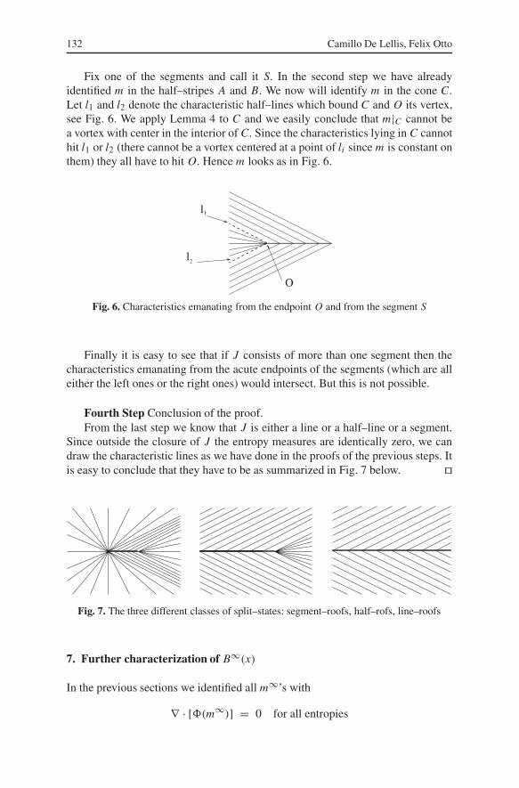
Fix one of the segments and call it S. In the second step we have alreadyidentified m in the half–stripes A and B. We now will identify m in the cone C.Let l1 and l2 denote the characteristic half–lines which bound C and O its vertex,see Fig. 6. We apply Lemma 4 to C and we easily conclude that m|C cannot bea vortex with center in the interior of C. Since the characteristics lying in C cannothit l1 or l2 (there cannot be a vortex centered at a point of li since m is constant onthem) they all have to hit O. Hence m looks as in Fig. 6.

Fig. 6. Characteristics emanating from the endpoint O and from the segment S

Finally it is easy to see that if J consists of more than one segment then thecharacteristics emanating from the acute endpoints of the segments (which are alleither the left ones or the right ones) would intersect. But this is not possible.

Fourth Step Conclusion of the proof.From the last step we know that J is either a line or a half–line or a segment.

Since outside the closure of J the entropy measures are identically zero, we candraw the characteristic lines as we have done in the proofs of the previous steps. Itis easy to conclude that they have to be as summarized in Fig. 7 below. ��

Fig. 7. The three different classes of split–states: segment–roofs, half–rofs, line–roofs

7. Further characterization of B∞(x)

In the previous sections we identified all m∞’s with

∇ · [�(m∞)] = 0 for all entropies


and all split–states, that is, m∞’s of the form

∇ · [�(m∞)] = T(�) ν∞ for all entropies.

So far, we have not made use of the fact that all these m∞’s come from theblow–up of a single field in a single point. This will be done now. We obtaina complete classification of B∞(x) for x ∈ G \ J in Proposition 6 and for x ∈ J inProposition 7. Before stating them we introduce a bit of terminology.

Definition 6. A vortex will be called

– centered if its unique point of singularity is the origin;– counterclockwise if it is of the form mv(x − x0) (see Definition 3(a));– clockwise if it is of the form −mv(x − x0).

A line–roof is centered if its singular line contains the origin.A half–roof is centered if its singular half–line starts from the origin.

Proposition 6. Let x ∈ G \ J (see the proof of Proposition 1 for the definition).Then

either B∞(x) contains only constantsor B∞(x) contains only the centered counterclockwise vortexor B∞(x) contains only the centered clockwise vortex.

Proposition 7. Let x ∈ J. Then

either B∞(x) contains only the centered line–roofor B∞(x) contains only the centered left half–roofor B∞(x) contains only the centered right half–roof.

Proof of Proposition 6. We recall from Proposition 1 that

B∞(x) contains only constants and vortices.

Without loosing our generality we assume that x = 0 and that m is definedeverywhere in B2(0).

First Step A functionalF on m–space.We will define a functionalF on all essentially bounded and weakly divergence–

free vector fields m on B2(0). Because m is divergence–free, there exists a Lipschitzcontinuous “stream function” ψ with ⊥∇ψ = m; ψ is unique up to additive con-stants. We take F(m) to be an “averaged second derivative” of ψ in the origin

F(m) := 3

2 π

∫B1(0)

(ψ(x) − ψ(0)) dx.

This functional is normalized such that |∇ψ|2 = 1 a.e. implies

F(m) ∈ [−1, 1]. (63)


We will be interested in how F behaves under rescaling. It is easy to check that

2 π

3

d

dr

∣∣∣∣r=1

[F(m0,r)

]

=∫

∂B1(0)

(ψ(x) − ψ(0)) dx − 3∫

B1(0)

(ψ(x) − ψ(0)) dx (64)

=∫

∂B1(0)

(ψ(x) − ψ(0) − 3

∫ 1

0(ψ(s x) − ψ(0)) s ds

)dx.

Second Step F separates the elements of B∞(0).We now state how F acts on m∞ ∈ B∞(0), i. e. on constants and vortices. We

list the obvious equivalences in the following table

F(m∞) = 1 centered counterclockwise vortexF(m∞) ∈ (0, 1) off–center counterclockwise vortexF(m∞) = 0 constantF(m∞) ∈ (−1, 0) off–center clockwise vortexF(m∞) = −1 centered clockwise vortex

We next state how F acts on rescaled versions m∞0,r of m∞ ∈ B∞(0):

F(m∞) ∈ (0, 1) ⇒ d

dr

∣∣∣∣r=1

[F(m∞

0,r

)]> 0, (65)

F(m∞) ∈ (−1, 0) ⇒ d

dr

∣∣∣∣r=1

[F(m∞

0,r

)]< 0.

Let us now argue in favor of, say, (65). In view of the table, F(m∞) ∈ (0, 1)

implies that m∞ is an off–center counterclockwise vortex. In particular, the relatedstream function ψ∞ is convex and we have

ψ∞(r x) − ψ∞(0) ≤ (ψ∞(x) − ψ∞(0)) r for x ∈ ∂B1 and r ∈ [0, 1].From the last line in (64) we see that d

dr

∣∣r=1

[F(m∞

0,r)]

is always nonnegative, andvanishes only if ψ∞ is homogeneous of degree 1 in B1(0). But this is not the casefor an off–center vortex. Hence (65) holds.

Third Step Compactness argument.We set for convenience

f(r) := F(m0,r) = 3

2 π

∫B1(0)

(ψ0,r(x) − ψ0,r(0)) dx

and observe that (see (64))

2 π

3r f ′(r) =

∫∂B1(0)

(ψ0,r(x) − ψ0,r(0)) dx

−3∫

B1(0)

(ψ0,r(x) − ψ0,r(0)) dx, (66)


where ψ0,r(x) − ψ0,r(0) = 1r (ψ(r x) − ψ(0)) is the stream function for m0,r . We

claim that for all δ > 0, there exist ε > 0, r0 > 0 s.t.

f(r) ∈ [δ, 1 − δ] and r ≤ r0 ⇒ r f ′(r) > ε, (67)

f(r) ∈ [−1 + δ,−δ] and r ≤ r0 ⇒ r f ′(r) < −ε.

We reason by contradiction in favor of (67) and assume that there exists a sequence{rn}n converging to zero such that

limn→∞ f(rn) ∈ (0, 1) and lim

n→∞ rn f ′(rn) ≤ 0. (68)

We may also assume that {m0,rn }n converges strongly to an m∞ ∈ B∞(0), whichimplies uniform convergence of {ψ0,rn }n to the corresponding ψ∞. Hence weobtain

F(m∞) = limn→∞ f(rn)

(68)∈ (0, 1),

d

dr

∣∣∣∣r=1

[F(m∞

0,r)] (64,66)= lim

n→∞ rn f ′(rn)(68)≤ 0.

This is a contradiction according to (65).

Fourth Step Ode argument.Since∫ r0

01r dr = ∞, (67) implies

lim infr↓0

f(r) < 1 − δ ⇒ lim supr↓0

f(r) ≤ δ. (69)

Indeed, it is obvious from (67) that

lim infr↓0

f(r) ≤ δ ⇒ lim supr↓0

f(r) ≤ δ (70)

lim infr↓0

f(r) ≤ 1 − δ ⇒ lim supr↓0

f(r) ≤ 1 − δ . (71)

We conclude from (70) that for proving (69) it is sufficient to show

lim infr↓0

f(r) ≤ δ.

We argue by contradiction: if this is false then for some ρ1 we have f(r) ∈ [δ,+∞[for any r ∈]0, ρ1]. But, taking into account (71) and the left–hand side of (69) wealso conclude that there exists ρ2 such that f(r) ∈] − ∞, 1 − δ] for any r ∈]0, ρ2].So if ρ = min{ρ1, ρ2} we would have f(r) ∈ [δ, 1 − δ] for all r ∈]0, ρ] andtherefore

+∞ > lim supt↓0

( f(ρ) − f(t)) ≥ lim supt↓0

∫ ρ

tf ′(r)dr

(67)≥ ε

∫ ρ

0

dr

r= +∞,

which is a contradiction.


Since δ > 0 was arbitrary (69) yields

lim infr↓0

f(r) < 1 ⇒ lim supr↓0

f(r) ≤ 0.

By symmetry, we also have

lim supr↓0

f(r) > −1 ⇒ lim infr↓0

f(r) ≥ 0.

Hence in view of (63), we only have three cases:

limr↓0

f(r) = 0 or limr↓0

f(r) = 1 or limr↓0

f(r) = −1.

HenceF(B∞(0)) either is {0}, {1}, or {−1}. In view of the above table, this impliesthe claim of the lemma. ��

Proof of Proposition 7. We recall that from Proposition 5 we know already

B∞(x) contains only constants, vortices and roofs (72)

B∞(x) contains at least one roof (73)

all roofs in B∞(x) have same triplet (ξ, m+, m−).

This last statement means that

– the direction of the set of discontinuity (which is a connected piece of a line)is determined by a vector ξ not depending on m;

– on this set any m ∈ B∞(x) jumps between two given values m− and m+ (andonly one possibility is given, i.e. fixed ξ as in Remark 3, m jumps from m− tom+ along ⊥ξ , while it cannot jump from m+ to m−).

By a change of coordinates, we may without loosing our generality assumex = 0 and ξ = (1, 0). Also, possibly passing to −m instead of m, we may assumethat

all roofs in B∞(x) are convex (74)

and, rescaling if necessary, that m is defined in all of B2(0).

First Step The functionalF .As in Proposition 6, ψ denotes the stream function of m: ⊥∇ψ = m. Let v+, v−

denote the vectors with ⊥v± = m±. Hence v± are the singled–out values of ∇ψ

in the line–roof case. We consider

F(m) :=∫ 1

0(ψ(s v+) + ψ(s v−) − 2 ψ(0)) ds


and observe that

d

dr

∣∣∣∣r=1

[F(m0,r)

]

= ψ(v+) + ψ(v−) − 2 ψ(0) − 2∫ 1

0(ψ(s v+) + ψ(s v−) − 2 ψ(0)) ds

= ψ(v+) − ψ(0) − 2∫ 1

0(ψ(s v+) − ψ(0)) ds

+ ψ(v−) − ψ(0) − 2∫ 1

0(ψ(s v−) − ψ(0)) ds. (75)

Second Step How functional F acts on B∞(0)

Let m∞ ∈ B∞(0) be given. It follows immediately from |∇ψ|2 = 1 a.e. that

F(m∞) ∈ [−1, 1]. (76)

In view of (72) we have

F(m∞)

{≥≤}

0 ⇒ ψ∞{

convexconcave

}. (77)

The directions v+, v− are just chosen such that F(m∞) = 1 for roofs m∞ whosesingular set (ridge) contains 0. Of course F(m∞) = ±1 is also true for a vortexm∞ with singular set (center) in 0. Hence in view of (72) we have

0 ∈ singular set ⇒ F(m∞) ∈ {−1, 1}. (78)

The converse statement

F(m∞) ∈ {−1, 1} ⇒ 0 ∈ singular set (79)

is also true: since |∇ψ|2 = 1 a.e. , F(m∞) ∈ {−1, 1} implies that ψ∞ is affinewith slope one along the segments [0, 1] v+ and [0, 1] v−. Assume that 0 ∈ sin-gular set. Then ∇ψ∞(0) exists so that the above translates into ∇ψ∞(0) · v+ =∇ψ∞(0) · v− = 1. Since v+ = v−, this yields |∇ψ∞(0)|2 > 1 — a contradiction.This establishes (79).

We now observe that there exists a c0 ∈ (0, 1) such that

ψ∞ linear ⇒ |F(m∞)| ≤ c0. (80)

Indeed, if ψ∞ is linear, we have F(m∞) = 12 (v+ + v−) · ∇ψ∞(0) and thus

|F(m∞)| ≤ | 12 (v+ + v−)| =: c0 because of |∇ψ∞(0)|2 = 1. Observe that c0 < 1

because of v+ = v−. This establishes (80). Finally, we have that

F(m∞) ∈ (c0, 1) ⇒ d

dr

∣∣∣∣r=1

[F(m∞

0,r

)]> 0, (81)

F(m∞) ∈ (−1,−c0) ⇒ d

dr

∣∣∣∣r=1

[F(m∞

0,r

)]< 0. (82)


Let us argue in favor of, say, (81). Since in particular F(m∞) ≥ 0 we have thatψ∞ is convex according to (77). Looking at (75), one realizes that as in the proofof Proposition 6, the convexity implies that d

dr

∣∣r=1

[F(m∞

0,r)] ≥ 0. It also shows

that equality, which we shall assume, can only occur if ψ∞ is affine along [0, 1] v+and [0, 1] v−. Since |F(m∞)| < 1, 0 is not in the singular set according to (78).Hence ∇ψ∞(0) exists and thus ψ∞ is affine on the union [0, 1] v+ ∪ [0, 1] v−of the two segments. Since F(m∞) only depends on the restriction of ψ∞ onto[0, 1] v+∪[0, 1] v−, we may apply (80), which yields |F(m∞)| ≤ c0 — the desiredcontradiction.

Third Step Conclusions from functionalFFrom (76, 81, 82), we obtain, by the same argument as in the proof of Propo-

sition 6, that

F(B∞(0)) = {1}, F(B∞(0)) = {−1} or F(B∞(0)) ⊂ [−c0, c0].The second case, i.e.F(B∞(0)) = {−1}, is easily ruled out: according to (77) thisimplies that for any m∞ ∈ B∞(0) ψ∞ is concave and according to (79) it impliesthat 0 is in its singular set. In view of (72, 74) this means that any m∞ ∈ B∞(x) isa vortex, which contradicts (73).

Also the third case, i.e. F(B∞(0)) ⊂ [−c0, c0], can be ruled out: accordingto (73) there exists an m∞ ∈ B∞(0) with non–empty singular set. Consider itsrescaled versions and their “blow–down” m∞,−∞:

m∞0,r

r↑∞−→ m∞,−∞.

A diagonal argument shows that also m∞,−∞ ∈ B∞(0). On the other hand, 0 mustbe in the singular set of m∞,−∞ so that |F(m∞,−∞)| = 1 in view of (78) — whichis in contradiction with F(B∞(0)) ⊂ [−c0, c0].

Hence we must have F(B∞(0)) = {1} which in view of (79), (77) and (74)translates into

B∞(0) contains only the centered counterclockwise vortexor roofs whose singular set runs through 0.

(83)

Fourth Step The functional GIn order to further restrict B∞(0), we introduce

G(m) := 2∫ 1

0(ψ(s (1, 0)) − ψ(0)) ds

and notice that

d

dr

∣∣∣∣r=1

[G(m0,r)

]

= 2(

ψ((1, 0)) − ψ(0) − 2∫ 1

0(ψ(s (1, 0)) − ψ(0)) ds

). (84)


Fifth Step How G acts on B∞(0).Let m∞ ∈ B∞(0) be given. We now list the properties which immediately

follow from (83)

G(m∞) ∈ [0, 1], (85)

G(m∞) = 1 ⇒ m∞ is the centered counterclockwise vortex

or the centered left half–roof, (86)

G(m∞) = 0 ⇒ m∞ is the centered line–roof

or the centered right half–roof. (87)

We also have

G(m∞) ∈ (0, 1) ⇒ d

dr

∣∣∣∣r=1

[G(m∞

0,r

)]> 0. (88)

Indeed, consider (84): The convexity of ψ∞ (guaranteed by (83)), implies as inProposition 6 that d

dr

∣∣r=1

[G(m∞

0,r)] ≥ 0 with equality only if ψ∞ is affine on the

segment [0, 1] (1, 0). In view of (83), affinity would imply ψ∞((1, 0))−ψ∞(0) ∈{0, 1} and therefore G(m∞) ∈ {0, 1} — a contradiction.

Sixth Step Conclusions from functional GAgain, we apply the argument from Proposition 6 and obtain from (85, 88) that

G(B∞(0)) = {1} or G(B∞(0)) = {0}.

In view of (86, 87), this means

either B∞(0) ⊂ {centered c.c. vortex, centered left half–roof}or B∞(0) ⊂ {centered line–roof, centered right half–roof}.

By symmetry, we also have

either B∞(0) ⊂ {centered c.c. vortex, centered right half–roof}or B∞(0) ⊂ {centered line–roof, centered left half–roof}.

The combination of both yields that B∞(0) either consists of the centeredcounterclockwise vortex, or the centered left half–roof, or the centered line–roof,or the centered right half–roof. Since the first case is not an option in view of (73),we obtain the claim of the proposition. ��

8. Rectifiability

In this section we will prove that the set J defined in Proposition 1 satisfies therequirements of Theorem 1. We recall that (9) has already been proved as point (d)of Proposition 1.


Proposition 8.

(a) J is rectifiable.(b) ForH1–a.e. x ∈ J there exist m+(x) and m−(x) such that

limr↓0

1

r2

{∫B+

r (x)|m(y) − m+(x)| dy

+∫

B−r (x)

|m(y) − m−(x)| dy

}= 0. (89)

(c) ForH1–a.e. x ∈ J we have

limr↓0

1

r2

∫Br(x)

|m(y) − mr |dy = 0. (90)

(d) If � is an entropy, then

µ� J = [η · (�(m+) − �(m−))]H1 J.

Proof. First Step Proof of (a).Let � be an entropy. Relation (21) and point (d) of Proposition 1 imply that

there exists a Borel function g� such that µ� = g�H1 J + µ, where µ(H ) = 0ifH1(H ) < ∞. Hence if we define ν := g�H1 J we have

µx,r� − νx,r

r

∗⇀ 0 forH1–a.e. x ∈ J . (91)

Proposition 7 implies that

µx,r�

r

∗⇀ c(x)H1 l(x) forH1–a.e. x ∈ J , (92)

where c(x) is a real number and l(x) is either a line which contains the origin ora half–line emanating from the origin.

Standard arguments imply that ‖ν‖ = |g�|H1 J and hence reasoning as inthe Sixth Step of the proof of Lemma 1 we conclude that

‖ν‖x,r − sign (g�(x))νx,r

r

∗⇀ 0 (93)

in every x which is a Lebesgue point for g� with respect to H1 J .Hence (92), (91) and (93) give

‖ν‖x,r

r

∗⇀ |c(x)|H1 l(x) for ‖ν‖–a.e. x. (94)

Since ‖ν‖ is a nonnegative measure this implies that

lim infr→0

‖ν‖(Br (x))

r= lim sup

r→0

‖ν‖(Br (x))

rfor ‖ν‖–a.e. x (95)


and that for ‖ν‖–a.e. x there exists a cone Cη(x) := {v : 2|v · η(x)| ≥ |v|} such that

lim supr→0

‖ν‖((x + Cη(x)) ∩ Br(x))

r= 0. (96)

Then it is a standard fact (see for example the Proof of Theorem 2.83 in [3]) that‖ν‖ is rectifiable (actually ‖ν‖ = |g�|H1 J and (96) are already sufficient forrectifiability: see Corollary 15.16 in [23]).

Hence we have that {g� = 0} ∩ J is a rectifiable set for any entropy �. Nowrecall the set of entropies C introduced in Warning 1. According to (36) and (28)we have

J ⊂⋃�∈C

{x : lim sup

r→0

‖µ�‖(Br(x))

r> 0}

. (97)

Hence we conclude

H1

((⋃�∈C

{g� = 0})

\ J

)= 0,

which proves the rectifiability of J .

Second Step Proof of (b).Proposition 7 implies that, forH1–a.e. x ∈ J , B∞(x) consists either of a single

line–roof or of a single half–line roof. But thanks to the rectifiability of J and to(97), forH1–a.e. x ∈ J we can find an entropy � such that

µx,r�

r

∗⇀ g�(x)H1 d(x)

where g�(x) = 0 and d(x) is the tangent line to J in x. In such an x, B∞(x) mustthen consist of a line–roof which jumps on d(x). This easily gives (89).

Third Step Proof of (c).We know from Proposition 6 that, for H1–a.e. x ∈ J , either B∞(x) consists

of constants, or it consists of a single centered vortex. If B∞(x) contains onlyconstants then for every sequence rn ↓ 0 we can extract a subsequence rh(n) suchthat

limn→∞

1

r2h(n)

∫Brh(n)

(x)|m(y) − mrh(n)

|dy = 0.

Thus in this case x satisfies (90). We will complete the proof by showing that

V := {x | B∞(x) consists of the centered counterclockwise vortex}is countable (the same holds for the clockwise vortex). Let mx denote the counter-clockwise vortex centered at x and define

δ :=∫

B1(x)∩B1(y)|mx(z) − my(z)|dz for |x − y| = 1.


A scaling argument yields∫

Bρ(x)∩Bρ(y)|mx(z) − my(z)|dz = δρ2 for |x − y| = ρ (98)

Hence the set

Vr :={

x :∫

Bρ(x)|m(z) − mx(z)|dz <

δρ2

2for every ρ ≤ r

}

is at most countable, because for x = y ∈ Vr we have |x − y| > r by (98) and thetriangle inequality. On the other hand we have by definition

V ⊂∞⋃

i=1

V 1i

so that also V is countable.

Fourth Step Proof of (d).Let � be a given entropy. By (b) we know that, for H1–a.e. x ∈ J , B∞(x)

consists of a line roof m∞x , jumping between the two values m+(x) and m−(x) on

the tangent line d(x) to J in x. Hence for these x we have

mx,r → m∞x strongly in L p

loc for p < ∞and thus

µx,r�

r

∗⇀ [η(x) · (�(m+(x)) − �(m−(x))]H1 d(x), (99)

where η(x) is the unit normal to J in x such that (89) holds.We recall again that thanks to relation (21) and point (d) of Proposition 1 we

have µ� J = g� J + µ where µ(H ) = 0 ifH1(H ) < ∞. Hence we have

µx,r�

r

∗⇀ g�(x)H1 d(x) forH1–a.e. x ∈ J . (100)

Comparing (100) with (99) we conclude that g�(x) = η(x) · (�(m+(x)) −�(m−(x)) forH1–a.e. x ∈ J . This completes the proof. ��

9. Final remarks

In this last section we show the fact which encouraged us to come with the argu-ments used in Sect. 7 and we also explain why the classification of Sect. 6 is stillnot sufficient for proving directly the rectifiability of J .

Bernd Kirchheim pointed out to us that the following result holds:

Theorem 2. Let ν = gH1 S for some S such that H1(S) < ∞ and moreoversuppose that for ν–a.e. x the weak limits of sequences of rescaled measures νx,rn /rn

with rn ↓ 0 can only be


(a) a constant c(x) times the Hausdorff measure concentrated on a line parallelto a fixed one (d(x));

(b) the zero measure.

Then S is rectifiable.

See [4] for a proof. The core of the argument is the fact that the measure H1

restricted to a line l is a monotone measure, i.e. for every x and every r < s

H1(l ∩ Br(x))

r≤ H1(l ∩ Bs(x))

s,

where the equality holds if and only if x ∈ l.Using known results in Geometric Measure Theory one can extend the previous

theorem substituting (a) with

(a’) a constant c > k(x) > 0 times the Hausdorff measure concentrated on someline d, where both c and d may depend freely on the chosen sequence {rn},whereas k(x) does not depend on it.

Also, see again [4], one could allow for a third possibility for the limits of rescaledmeasures, namely

(c) a constant c times the Hausdorff measure concentrated on some half–line d(where, as in (a’), d is allowed to vary among all half–lines and c is onlysubject to the constraint c > k(x) > 0).

Anyway it is not clear to us if the same could hold allowing the rescaledmeasures to possibly converge also to segments. We are here very near to a border–line between rectifiability and unrectifiability. Indeed let us take the measure ν

given by the restriction ofH1 to the graph of the function

f(x) :=∞∑

i=1

2−n2χAn (x),

being An the union of the closed segments[(

k − 2−[log n]) 2−n2, k2−n2

], where

k ∈ {1, 2, . . . , 2n2} and [x] denotes the integer part of x. This example is a slightmodification of one shown by Dickinson in [14] and it can be proved that

(i) ν is not rectifiable (i.e. the graph of f is an unrectifiable set);(ii) for ν–a.e. x, if the measures νx,rn /rn converge then their weak limit is given

by H1 restricted to a subset J of {(x, y), x ∈ R} for some y ∈ R (where ydepends on the sequence {rn});

(iii) the subsets J which appear in (ii) consist all of at most two connected com-ponents (more precisely they can be the full line, an half–line, a segment, thefull line minus a segment or the empty set).

The proofs of these facts are just a routine modification of those present in [14].


References

1. Alouges, F., Rivière, T., Serfaty, S.: Wall energies of micromagnetic materials withstrong planar anisotropy. ESAIM, Control Optim. Calc. Var. 8, 31–68 (2002)

2. Ambrosio, L., De Lellis, C., Mantegazza, C.: Line energies for gradient vector fields inthe plane. Calc. Var. Partial Differ. Equ. 9, 327–355 (1999)

3. Ambrosio, L., Fusco, N., Pallara, D.: Functions of bounded variation and free discon-tinuity problems. Oxford Mathematical Monographs. Oxford: Clarendon Press 2000

4. Ambrosio, L., Kirchheim, B., Lecumberry, M., Rivière, T.: The local structure of NéelWalls. To appear in the Volume dedicated to the 80th birthday of O. Ladyzhenskaya.Kluwert Academic 2002

5. Ambrosio, L., Lecumberry, M., Rivière, T.: Viscosity property of minimizing micro-magnetic configurations. To appear in Commun. Pure Appl. Math.

6. Aviles, P., Giga, Y.: A mathematical problem related to the physical theory of liquidcrystals configurations. Proc. Centre Math. Anal. Austral. Nat. Univ. 12, 1–16 (1987)

7. Aviles, P., Giga, Y.: On lower semicontinuity of a defect energy obtained by a singularlimit of the Ginzburg-Landau type energy for gradient fields. Proc. R. Soc. Edinb., Sect.A, Math. 129, 1–17 (1999)

8. Ben Belgacem, H., Conti, S., De Simone, A., Müller, S.: Energy scaling of compressedelastic films: three–dimensional elasticity and reduced theories. Arch. Ration. Mech.Anal. 164, 1–37 (2002)

9. De Lellis, C.: Energie di linea per campi di gradienti. Ba. D. Thesis. University of Pisa1999

10. De Lellis, C.: An example in the gradient theory of phase transitions. ESAIM, ControlOptim. Calc. Var. 7, 285–289 (2002)

11. De Lellis, C., Otto, F., Westdickenberg, M.: Structure of entropy solutions for multi–dimensional scalar conservation laws.Preprint Nr. 95/2002 at http://www.mis.mpg.de/preprints

12. De Simone, A., Kohn, R.V., Müller, S., Otto, F.: A reduced theory for thin–film micro-magnetics. Commun. Pure Appl. Math. 55, 1408–1460 (2002)

13. De Simone, A., Kohn, R.V., Müller, S., Otto, F.: A compactness result in the gradienttheory of phase transition. Proc. R. Soc. Edinb., Sect. A, Math. 131, 833–844 (2001)

14. Dickinson, D.R.: Study or extreme cases with respect to densities of irregular linearlymeasurable plane sets of points. Math. Ann. 116, 358–373 (1939)

15. Di Perna, R., Lions, P.L., Meyer, Y.: L p regularity of velocity averages. Ann. Inst. HenriPoincaré, Anal. Non Linéaire 8, 271–287 (1991)

16. Federer, H.: Geometric measure theory. Classics in Mathematics. Berlin, Heidelberg,New York: Springer 1969

17. Jabin, P.E., Otto, F., Perthame, B.: Line–energy Ginzburg–Landau models: zero–energystates. Ann. Sc. Norm. Super. Pisa, Cl. Sci., V. Ser. 1, 187–202 (2002)

18. Jabin, P.E., Perthame, B.: Compactness in Ginzburg–Landau energy by kinetic averag-ing. Commun. Pure Appl. Math. 54, 1096–1109 (2001)

19. Jin, W., Kohn, R.V.: Singular perturbation and the energy of folds. J. Nonlinear Sci. 10,355–390 (2000)

20. Kruzkov, S.N.: First order quasilinear equations in several independent variables. Math.USSR–Sbornik 10, 217–243 (1970)

21. Lecumberry, M., Rivière, T.: Regularity property for Micromagnetic configurationshaving zero jump energy. To appear in Calc. Var. Partial Differ. Equ.

22. Lions, P.L., Perthame, B., Tadmor, E.: A kinetic formulation of multidimensional scalarconservation laws and related questions. J. Am. Math. Soc. 7, 169–191 (1994)

23. Mattila, P.: Geometry of sets and measures in Euclidean spaces. Fractal and rectifiability.Cambridge Studies in Advanced Mathematics. Cambridge: Cambridge University Press1995

24. Ortiz, M., Gioia, G.: The morphology and folding patterns of bucking driven thin–filmblisters. J. Mech. Phys. Solids 42, 531–559 (1994)


25. Rivière, T., Serfaty, S.: Compactness, kinetic formulation and entropies for a problemrelated to Micromagnetics. To appear in Commun. Partial Differ. Equations

26. Rivière, T., Serfaty, S.: Limiting domain wall energy for a problem related to micro-magnetics. Commun. Pure Appl. Math. 54, 294–338 (2001)

structure of entropy solutions to the eikonal equation

Documents