studies of phonon anharmonicity in solids
TRANSCRIPT
Studies of Phonon Anharmonicity in Solids
Thesis by
Tian Lan
In Partial Fulfillment of the Requirements
for the Degree of
Doctor of Philosophy
California Institute of Technology
Pasadena, California
2014
(Defended May 6, 2014)

ii
© 2014
Tian Lan
All Rights Reserved

iii
Acknowledgements
It is almost mission impossible to express my gratitude to all the wonderful
people I have had the pleasure of meeting and knowing during my time at Caltech.
I have been so fortunate to have Brent Fultz as my research advisor. Brent has
provided enormous encouragement, guidance, patience and support for my study.
This work would not have been possible without his mentorship.
I appreciate the support from my committee: Bill Johnson, Bill Goddard, George
Rossman, Keith Schwab and Rudy Marcus. In particular, I thank George for his
guidance in my experimental work and kindness in sharing with me wonderful
equipments from his lab.
I would like to thank all current and former members of the Fultz group,
who have been a constant source of thoughts and support: Olivier Delaire, Jiao
Lin, Channing Ahn, Hongjin Tan, Xiaoli Tang, Jorge Munoz, Nick Stadie, David
Abrecht, Lisa Mauger, Hillary Smith, Sally Tracy, Dennis Kim, Max Murialdo,
Jane Herriman, and Nick Weadock. Special thanks to Chen Li, who gave me the
initiation class on Raman spectrometry and computational physics.
I also wish to thank all the members of the Caltech community who have helped
me over the years: especially, Sandra Troian, for her support when I met difficulties
in the beginning of my graduate research; Mike Vondrus, for his dexterousness in
building the crazy things I designed; Avalon Johnson, for maintaining the group
cluster, and helping me solve problems in running the computation scripts; Ali
Ghaffari, for teaching me nano-fabrication; Qi An, for his informative suggestions
about first principles calculations; Pam Albertson and many other staff in Depart-
ment of Applied Physics and Materials Science, for their efforts to keep everything
iv
running.
I wish to acknowledge the generous help and support of our collaborators at Oak
Ridge National Laboratory: Doug Abernathy, Jen Niedziela and Matthew Stone,
among many others. They made our inelastic neutron scattering experiments
possible.
Finally, I wish to express my gratitude to my dear family, my parents, Jiasheng
and Fang, and my wife, Zhaoyan, for their unconditional support and love through
the years. And Raymond, you bring us the paramount joy.

v
Abstract
Today our understanding of the vibrational thermodynamics of materials at low
temperatures is emerging nicely, based on the harmonic model in which phonons
are independent. At high temperatures, however, this understanding must ac-
commodate how phonons interact with other phonons or with other excitations.
We shall see that the phonon-phonon interactions give rise to interesting coupling
problems, and essentially modify the equilibrium and non-equilibrium properties
of materials, e.g., thermodynamic stability, heat capacity, optical properties and
thermal transport of materials. Despite its great importance, to date the anhar-
monic lattice dynamics is poorly understood and most studies on lattice dynamics
still rely on the harmonic or quasiharmonic models. There have been very few
studies on the pure phonon anharmonicity and phonon-phonon interactions. The
work presented in this thesis is devoted to the development of experimental and
computational methods on this subject.
Modern inelastic scattering techniques with neutrons or photons are ideal for
sorting out the anharmonic contribution. Analysis of the experimental data can
generate vibrational spectra of the materials, i.e., their phonon densities of states
or phonon dispersion relations. We obtained high quality data from laser Raman
spectrometer, Fourier transform infrared spectrometer and inelastic neutron spec-
trometer. With accurate phonon spectra data, we obtained the energy shifts and
lifetime broadenings of the interacting phonons, and the vibrational entropies of
different materials. The understanding of them then relies on the development of
the fundamental theories and the computational methods.
We developed an efficient post-processor for analyzing the anharmonic vibra-
vi
tions from the molecular dynamics (MD) calculations. Currently, most first prin-
ciples methods are not capable of dealing with strong anharmonicity, because the
interactions of phonons are ignored at finite temperatures. Our method adopts
the Fourier transformed velocity autocorrelation method to handle the big data
of time-dependent atomic velocities from MD calculations, and efficiently recon-
structs the phonon DOS and phonon dispersion relations. Our calculations can
reproduce the phonon frequency shifts and lifetime broadenings very well at vari-
ous temperatures.
To understand non-harmonic interactions in a microscopic way, we have devel-
oped a numerical fitting method to analyze the decay channels of phonon-phonon
interactions. Based on the quantum perturbation theory of many-body interactions,
this method is used to calculate the three-phonon and four-phonon kinematics sub-
ject to the conservation of energy and momentum, taking into account the weight
of phonon couplings. We can assess the strengths of phonon-phonon interactions
of different channels and anharmonic orders with the calculated two-phonon DOS.
This method, with high computational efficiency, is a promising direction to ad-
vance our understandings of non-harmonic lattice dynamics and thermal transport
properties.
These experimental techniques and theoretical methods have been successfully
performed in the study of anharmonic behaviors of metal oxides, including rutile
and cuprite stuctures, and will be discussed in detail in Chapters 4 to 6. For exam-
ple, for rutile titanium dioxide (TiO2), we found that the anomalous anharmonic
behavior of the B1g mode can be explained by the volume effects on quasiharmonic
force constants, and by the explicit cubic and quartic anharmonicity. For rutile
tin dioxide (SnO2), the broadening of the B2g mode with temperature showed an
unusual concave downwards curvature. This curvature was caused by a change
with temperature in the number of down-conversion decay channels, originating
with the wide band gap in the phonon dispersions. For silver oxide (Ag2O), strong
anharmonic effects were found for both phonons and for the negative thermal
expansion.

vii
Contents
Acknowledgements iii
Abstract v
1 Lattice Dynamics and Phonon-Phonon Interactions 1
1.1 Bravais Lattices . . . . . . . . . . . . . . . . . . . . . . . . . . . . . . . 2
1.2 Harmonic Lattice Dynamics . . . . . . . . . . . . . . . . . . . . . . . . 3
1.3 Quasiharmonic Approximation . . . . . . . . . . . . . . . . . . . . . . 5
1.4 Anharmonic Lattice Dynamics . . . . . . . . . . . . . . . . . . . . . . 6
1.5 Green’s Function Method . . . . . . . . . . . . . . . . . . . . . . . . . 7
1.5.1 The Retarded Green’s Function and Lehmann Representation 7
1.5.2 Perturbation Theory and Wick’s Theorem For Finite Temper-
atures . . . . . . . . . . . . . . . . . . . . . . . . . . . . . . . . . 9
1.6 Phonon-Phonon Interactions and Phonon Lifetime . . . . . . . . . . . 13
1.7 Self-Consistent Lattice Dynamics . . . . . . . . . . . . . . . . . . . . . 15
2 Experimental Methods 17
2.1 Raman Scattering . . . . . . . . . . . . . . . . . . . . . . . . . . . . . . 18
2.1.1 Introduction . . . . . . . . . . . . . . . . . . . . . . . . . . . . . 18
2.1.2 The Frequency Resolved Raman Spectroscopy . . . . . . . . . 19
2.1.2.1 Classical Theory . . . . . . . . . . . . . . . . . . . . . 19
2.1.2.2 Quantum Theory and Placzek’s Approximation . . . 21
2.1.2.3 Loudon’s Third Order Perturbation Theory . . . . . 25
2.1.3 Group Theory and Selection Rules . . . . . . . . . . . . . . . . 27

viii
2.1.3.1 Classical Approach . . . . . . . . . . . . . . . . . . . 27
2.1.3.2 Group Theoretical Approach . . . . . . . . . . . . . . 28
2.1.3.3 The Correlation Method . . . . . . . . . . . . . . . . 30
2.2 Time of Flight Inelastic Neutron Scattering . . . . . . . . . . . . . . . 33
2.2.1 Introduction . . . . . . . . . . . . . . . . . . . . . . . . . . . . . 33
2.2.2 Basic Principles . . . . . . . . . . . . . . . . . . . . . . . . . . . 33
2.2.2.1 Scattering Cross Section . . . . . . . . . . . . . . . . . 33
2.2.2.2 Coherent and Incoherent Scattering . . . . . . . . . . 34
2.2.3 Wide Angular-Range Chopper Spectrometer (ARCS) . . . . . 36
2.2.4 Data Reduction . . . . . . . . . . . . . . . . . . . . . . . . . . . 37
3 Computational Methodologies 39
3.1 Density Functional Theory . . . . . . . . . . . . . . . . . . . . . . . . 40
3.1.1 Introduction . . . . . . . . . . . . . . . . . . . . . . . . . . . . . 40
3.1.2 Hohenberg-Kohn Theorems . . . . . . . . . . . . . . . . . . . . 40
3.1.3 Kohn-Sham Theory . . . . . . . . . . . . . . . . . . . . . . . . . 41
3.1.4 Functionals for Exchange and Correlation . . . . . . . . . . . . 42
3.1.5 Pseudopotentials . . . . . . . . . . . . . . . . . . . . . . . . . . 44
3.2 Molecular Dynamics Methods . . . . . . . . . . . . . . . . . . . . . . . 45
3.2.1 Introduction . . . . . . . . . . . . . . . . . . . . . . . . . . . . . 45
3.2.2 Solving Equations of Motion . . . . . . . . . . . . . . . . . . . 46
3.2.3 Ensembles . . . . . . . . . . . . . . . . . . . . . . . . . . . . . . 47
3.3 Phonon Calculations . . . . . . . . . . . . . . . . . . . . . . . . . . . . 48
3.3.1 Introduction . . . . . . . . . . . . . . . . . . . . . . . . . . . . . 48
3.3.2 Lattice Dynamics Approach . . . . . . . . . . . . . . . . . . . . 48
3.3.2.1 Small Displacement Method . . . . . . . . . . . . . . 48
3.3.2.2 Density Functional Perturbation Method . . . . . . . 50
3.3.3 Molecular Dynamics Approach . . . . . . . . . . . . . . . . . . 51
3.3.3.1 Time-Correlation Method . . . . . . . . . . . . . . . . 51
3.3.3.2 Fourier-Transformed Velocity Autocorrelation Method 52
ix
3.4 Anharmonic Fitting Algorithm . . . . . . . . . . . . . . . . . . . . . . 55
4 Phonon Anharmonicity of Rutile TiO2 57
4.1 Introduction . . . . . . . . . . . . . . . . . . . . . . . . . . . . . . . . . 58
4.2 Experiments . . . . . . . . . . . . . . . . . . . . . . . . . . . . . . . . . 60
4.3 Molecular Dynamics Calculations . . . . . . . . . . . . . . . . . . . . 61
4.4 Results . . . . . . . . . . . . . . . . . . . . . . . . . . . . . . . . . . . . 63
4.4.1 Experiment . . . . . . . . . . . . . . . . . . . . . . . . . . . . . 63
4.4.2 MD Simulations . . . . . . . . . . . . . . . . . . . . . . . . . . . 66
4.5 Experimental Data Analysis . . . . . . . . . . . . . . . . . . . . . . . . 67
4.5.1 Analysis of Quasiharmonicity and Anharmonicity . . . . . . . 67
4.5.2 Analysis of Cubic and Quartic Anharmonicity . . . . . . . . . 70
4.6 Discussion . . . . . . . . . . . . . . . . . . . . . . . . . . . . . . . . . . 80
4.6.1 Anharmonicities from Experimental Trends . . . . . . . . . . . 80
4.6.2 Anharmonicities from MD Simulations . . . . . . . . . . . . . 82
4.6.3 Vibrational Entropy of Rutile TiO2 . . . . . . . . . . . . . . . . 89
4.7 Conclusions . . . . . . . . . . . . . . . . . . . . . . . . . . . . . . . . . 90
5 Phonon Anharmonicity of Rutile SnO2 92
5.1 Introduction . . . . . . . . . . . . . . . . . . . . . . . . . . . . . . . . . 93
5.2 Experimental Procedures . . . . . . . . . . . . . . . . . . . . . . . . . . 95
5.3 Results . . . . . . . . . . . . . . . . . . . . . . . . . . . . . . . . . . . . 96
5.4 Calculations . . . . . . . . . . . . . . . . . . . . . . . . . . . . . . . . . 100
5.4.1 First Principles Lattice Dynamics . . . . . . . . . . . . . . . . . 100
5.4.2 The Kinematic Functionals Dω(Ω) and Pω(Ω) . . . . . . . . . . 102
5.5 Analysis . . . . . . . . . . . . . . . . . . . . . . . . . . . . . . . . . . . 103
5.5.1 Separating Anharmonicity from Quasiharmonicity . . . . . . 103
5.5.2 Cubic and Quartic Anharmonicity . . . . . . . . . . . . . . . . 105
5.6 Discussion . . . . . . . . . . . . . . . . . . . . . . . . . . . . . . . . . . 110
5.7 Conclusions . . . . . . . . . . . . . . . . . . . . . . . . . . . . . . . . . 112
x
6 Phonon Anharmonicity of Ag2O with Cuprite Structure 113
6.1 Introduction . . . . . . . . . . . . . . . . . . . . . . . . . . . . . . . . . 114
6.2 Experiments . . . . . . . . . . . . . . . . . . . . . . . . . . . . . . . . . 118
6.2.1 Inelastic Neutron Scattering . . . . . . . . . . . . . . . . . . . . 118
6.2.2 Fourier Transform Far-Infrared Spectrometer . . . . . . . . . . 118
6.2.3 Results . . . . . . . . . . . . . . . . . . . . . . . . . . . . . . . . 120
6.3 First-Principles Molecular Dynamics Simulations . . . . . . . . . . . . 121
6.3.1 Methods . . . . . . . . . . . . . . . . . . . . . . . . . . . . . . . 121
6.3.2 Results . . . . . . . . . . . . . . . . . . . . . . . . . . . . . . . . 126
6.4 Anharmonic Perturbation Theory . . . . . . . . . . . . . . . . . . . . . 131
6.4.1 Computational Methodology . . . . . . . . . . . . . . . . . . . 131
6.4.2 Results . . . . . . . . . . . . . . . . . . . . . . . . . . . . . . . . 132
6.5 Discussion . . . . . . . . . . . . . . . . . . . . . . . . . . . . . . . . . . 135
6.5.1 Quasiharmonic Approximation . . . . . . . . . . . . . . . . . . 135
6.5.2 Negative Thermal Expansion . . . . . . . . . . . . . . . . . . . 139
6.5.3 Explicit Anharmonicity . . . . . . . . . . . . . . . . . . . . . . 140
6.6 Conclusions . . . . . . . . . . . . . . . . . . . . . . . . . . . . . . . . . 141
7 Conclusions 143
7.1 Summary . . . . . . . . . . . . . . . . . . . . . . . . . . . . . . . . . . . 143
7.2 Future Work . . . . . . . . . . . . . . . . . . . . . . . . . . . . . . . . . 145
A The evaluation of the 2nd order Feynman diagram of phonon-phonon
interactions 150
B The Corrrelation method: an example for Ag2O with curprite structure 154
C Raman spectra of two-phase and solid solution phase of Li0.6FePO4 at
elevated temperatures 158
Bibliography 161
xi
List of Figures
1.1 Dyson’s equation . . . . . . . . . . . . . . . . . . . . . . . . . . . . . . . 12
1.2 The lowest order terms of the proper self energy . . . . . . . . . . . . . 13
2.1 Schematic energy level diagram showing the states involved in Raman
signal. . . . . . . . . . . . . . . . . . . . . . . . . . . . . . . . . . . . . . 24
2.2 Schematic overview of the ARCS design with components labeled [13] 37
3.1 The flow chart implementing the Fourier-transformed velocity auto-
correlation method . . . . . . . . . . . . . . . . . . . . . . . . . . . . . . 55
4.1 Rutile structure and oxygen atom displacements for Raman-active
modes. . . . . . . . . . . . . . . . . . . . . . . . . . . . . . . . . . . . . . 60
4.2 Raman spectra of rutile TiO2 at selected temperatures from 100 K to
1150 K. . . . . . . . . . . . . . . . . . . . . . . . . . . . . . . . . . . . . . 64
4.3 Temperature dependence of (a) frequency shifts, (b) FWHM, of the
Raman modes B1g, Eg and A1g. Data of Ref. [ [59]] are shown as open
triangles in panel a. . . . . . . . . . . . . . . . . . . . . . . . . . . . . . . 65
4.4 (a) The B1g Raman peak calculated from the velocity trajectories of
MD simulations, at temperatures as labeled and constant pressure
of 0 GPa, and at pressures from 0 to 6 GPa at 300 K. (b) Calculated
Eg Raman peak, and (c) Calculated A1g Raman peak at temperatures
as labeled and constant pressure of 0 GPa. Solid red curves are the
Lorentzian fits. . . . . . . . . . . . . . . . . . . . . . . . . . . . . . . . . 68
xii
4.5 (a) Two-phonon density of states D(Ω) of Eq. 4.9 for 300 K (black) and
1000 K (red). The up-conversion and down-conversion contributions
to D(Ω) at 1000 K are shown in green dash and red dash curves,
respectively. The overtone process at 1000 K is highlighted as the
filled area under the blue curve. (b) P(Ω) of Eq. 5.2 at 300 K (black)
and 1000 K (red). . . . . . . . . . . . . . . . . . . . . . . . . . . . . . . . 76
4.6 Temperature dependence of parameters for fittings to Raman peaks of
mode B1g (a) frequency shift, and (b) FWHM. Solid circles are experi-
mental data. Solid curves are the fittings of the experimental points to
Eq. 4.5 and Eq. 4.11d. Dotted line is the quasiharmonic contribution
to the frequency shift. Dash-dot line is the explicit anharmonicity
ω0 + ∆(4) + ∆(3), and dashed line is ω0 + ∆
(3). . . . . . . . . . . . . . . . . 77
4.7 Temperature dependence of parameters for fittings to Raman peaks
of mode Eg (a) frequency shift, and (b) FWHM. Dotted line is the
quasiharmonic contribution to the frequency shifts. Dash-dot line is
the explicit anharmonicity ω0 + ∆(4) + ∆(3) and dashed line is ω0 + ∆
(3). 78
4.8 Temperature dependence of parameters for fittings to Raman peaks
of mode A1g (a) frequency shift, and (b)FWHM. Dotted line represents
the quasiharmonic contribution to the frequency shifts. Dash-dot line
is the explicit anharmonicity ω0 + ∆(4) + ∆(3) + ∆(3′), short dash line
corresponds to ω0 + ∆(3) + ∆(3′) and dashed line is ω0 + ∆
(3). . . . . . . 79
4.9 (a) Temperature dependent frequency shift, (b) FWHM broadening,
and (c) pressure dependent frequency shift, of the B1g mode from MD
calculations (red), compared with experiment data (black). . . . . . . . 84
xiii
4.10 Frozen phonon potential of the B1g mode calculated with the MW
shell model, and its response to the volume increase (indicated as
the dash arrow). The potential is decomposed into the harmonic
component and quartic component. The three potentials are for lattice
parameters corresponding to 300 K at 0 GPa (black), 300 K at 6 GPa
(blue), and 800 K at 0 GPa (red). The inset shows the B1g mode of
rutile TiO2 structure projected along the c-axis. Small arrows indicate
the polarization vectors of this mode. . . . . . . . . . . . . . . . . . . . 86
4.11 Temperature dependence of the (a) frequency shift, and (b) FWHM
broadening, of the Eg mode from MD simulations (red) and experi-
mental data (black). . . . . . . . . . . . . . . . . . . . . . . . . . . . . . . 87
4.12 Temperature dependence of the (a) frequency shift, and (b) FWHM
broadening, of the A1g mode from MD simulations (red) and experi-
mental data (black). . . . . . . . . . . . . . . . . . . . . . . . . . . . . . 88
4.13 Ratio of the mode anharmonic potential and harmonic potential, with
increasing temperature. . . . . . . . . . . . . . . . . . . . . . . . . . . . 89
5.1 Rutile structure and oxygen atom displacements for Raman-active
modes. . . . . . . . . . . . . . . . . . . . . . . . . . . . . . . . . . . . . . 94
5.2 Raman spectra of powder samples of rutile SnO2 at selected temper-
atures. . . . . . . . . . . . . . . . . . . . . . . . . . . . . . . . . . . . . . 98
5.3 Temperature dependence of (a) frequency shifts, (b) breadths as FWHMs,
of the Raman modes Eg, A1g and B2g. The solid and open symbols rep-
resent the experimental data from powder and single crystal samples,
respectively. Solid curves are the theoretical fittings with a full calcu-
lation of the kinematics of three- phonon and four-phonon processes.
The dashed curve was calculated without considering the frequency
dependence of D0↓(Ω), the number of decay channels, at elevated
temperatures. . . . . . . . . . . . . . . . . . . . . . . . . . . . . . . . . . 99
xiv
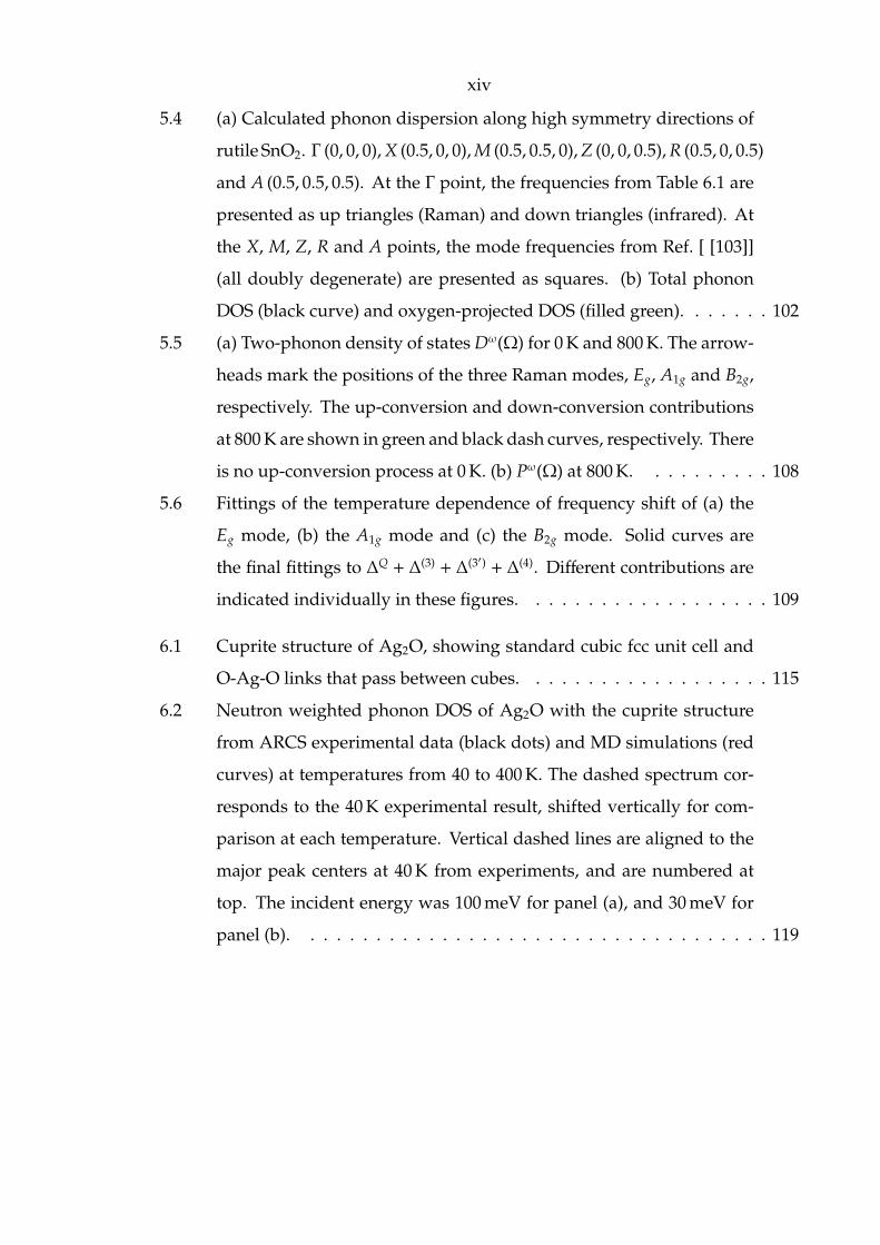
5.4 (a) Calculated phonon dispersion along high symmetry directions of
rutile SnO2. Γ (0, 0, 0), X (0.5, 0, 0), M (0.5, 0.5, 0), Z (0, 0, 0.5), R (0.5, 0, 0.5)
and A (0.5, 0.5, 0.5). At the Γ point, the frequencies from Table 6.1 are
presented as up triangles (Raman) and down triangles (infrared). At
the X, M, Z, R and A points, the mode frequencies from Ref. [ [103]]
(all doubly degenerate) are presented as squares. (b) Total phonon
DOS (black curve) and oxygen-projected DOS (filled green). . . . . . . 102
5.5 (a) Two-phonon density of states Dω(Ω) for 0 K and 800 K. The arrow-
heads mark the positions of the three Raman modes, Eg, A1g and B2g,
respectively. The up-conversion and down-conversion contributions
at 800 K are shown in green and black dash curves, respectively. There
is no up-conversion process at 0 K. (b) Pω(Ω) at 800 K. . . . . . . . . . 108
5.6 Fittings of the temperature dependence of frequency shift of (a) the
Eg mode, (b) the A1g mode and (c) the B2g mode. Solid curves are
the final fittings to ∆Q + ∆(3) + ∆(3′) + ∆(4). Different contributions are
indicated individually in these figures. . . . . . . . . . . . . . . . . . . 109
6.1 Cuprite structure of Ag2O, showing standard cubic fcc unit cell and
O-Ag-O links that pass between cubes. . . . . . . . . . . . . . . . . . . 115
6.2 Neutron weighted phonon DOS of Ag2O with the cuprite structure
from ARCS experimental data (black dots) and MD simulations (red
curves) at temperatures from 40 to 400 K. The dashed spectrum cor-
responds to the 40 K experimental result, shifted vertically for com-
parison at each temperature. Vertical dashed lines are aligned to the
major peak centers at 40 K from experiments, and are numbered at
top. The incident energy was 100 meV for panel (a), and 30 meV for
panel (b). . . . . . . . . . . . . . . . . . . . . . . . . . . . . . . . . . . . 119

xv
6.3 Shifts of centers of peaks in the phonon DOS, relative to data at 40 K.
The filled symbols are experimental data, open symbols (green) are
from MD-based QHA calculations and solid curves (red) are from MD
calculations. Indices 1, 2, 3 correspond to the peak labels in Fig. 6.2,
and are also represented by the triangle, square and circle respectively
for experimental data and QHA calcuations. . . . . . . . . . . . . . . . 120
6.4 (a) FT-IR absorbtion spectra of Ag2O with the cuprite structure at
300 K. (b), (c) Enlargement of two bands at selected temperatures. . . . 122
6.5 The phonon densities of states for two different cells used in molecular
dynamics simulations at 400 K. . . . . . . . . . . . . . . . . . . . . . . . 125
6.6 The simulated phonon densities of states for 12, 18 and 30 ps at 40 K . 125
6.7 Temperature dependence of lattice parameter from experimental data
in Ref. [ [111]], quasiharmonic calculations and MD calculations,
expressed as the relative changes with respect to their 40 K values,
i.e., a(T)/a(40 K) − 1. . . . . . . . . . . . . . . . . . . . . . . . . . . . . . 127
6.8 Phonon modes simulated by MD and projected on the Γ-point, at
temperatures and pressures as labeled. The normal-mode frequen-
cies calculated from harmonic lattice dynamics are shown as vertical
dashed lines in red. The group symmetry for each mode is shown at
the bottom. . . . . . . . . . . . . . . . . . . . . . . . . . . . . . . . . . . 129
6.9 (a) Temperature dependent frequency shifts of the Ag-dominated F(1)1u
mode and the O-dominated F2g and F(2)1u modes from FT-IR (black),
compared with the MD simulated peaks (red) such as in Fig. 6.8. (b)
The lifetimes of the corresponding modes at temperatures from 40 to
400 K, from FT-IR (black) and the MD simulated peaks (red). . . . . . 130
6.10 (a) Calculated phonon dispersion along high-symmetry directions of
Ag2O with the cuprite structure. Γ (0, 0, 0), M (0.5, 0.5, 0), X (0.5, 0, 0),
R (0.5, 0.5, 0.5). (b) The TDOS spectra, D(ω), at 40 K (dashed) and
400 K (solid). The down-conversion and up-conversion contributions
are presented separately as black and green curves, respectively. . . . 134

xvi
6.11 Temperature dependence of the inverse of the quality factors 1/Q for
the F(1)1u , A2u, F2g and F(2)
1u phonon modes from FT-IR (black squares),
MD calculations(red circles) and the theoretical fittings with a full
calculation of the TDOS. The unit of the fitting parameter |C(3)j |2 is 10−1
eV−1. . . . . . . . . . . . . . . . . . . . . . . . . . . . . . . . . . . . . . . 135
6.12 Neutron weighted phonon DOS of Ag2O with the cuprite structure
from MD simulations. The green spectrum is the MD simulated
phonon DOS at 40 K and 0.45 GPa. Vertical dashed lines are aligned
to the major peak centers at 40 K and labeled by numbers. The inci-
dent energy was 100 meV for panel (a), and 30 meV for panel (b). The
spectra were convoluted with the resolution function characteristic of
ARCS for the different energies of the incident neutron beam. . . . . . 138
A.1 Coutour of evaluation for energy sums . . . . . . . . . . . . . . . . . . 150
C.1 Raman spectra at elevated temperatures of two-phase Li0.6FePO4 (left
panel) and solid solution phase quenched at 400 C(right panel) . . . . 159
C.2 Raman spectra of two-phase Li0.6FePO4 right above the phase transi-
tion temperature at 260 C but with different heating times. . . . . . . 160
xvii
List of Tables
4.1 Properties of rutile TiO2 from present calculations, compared to ex-
perimental data. Units: lattice parameters in Å, Raman frequencies
in cm−1, thermal expansion coefficients in 10−6K−1, volume compress-
ibility in 10−3GPa−1. . . . . . . . . . . . . . . . . . . . . . . . . . . . . . 66
4.2 Frequencies of the three Raman modes, their logarithmic pressure
and temperature derivatives, and mode Gruneisen parameters. The
measured isobaric temperature derivatives are separated into the pure
volume and pure temperature contributions. Samara and Peercy’s
results are listed in the lower row for each mode. And mode Gruneisen
parameters are from Ref. [59] . . . . . . . . . . . . . . . . . . . . . . . . 70
4.3 Fitting parameters for the temperature dependent Raman modes (unit:
1011 erg−1) . . . . . . . . . . . . . . . . . . . . . . . . . . . . . . . . . . . 80
4.4 Entropy in J/(mol K) of rutile TiO2 from MD calculations and experi-
mental data of Ref. [95]. . . . . . . . . . . . . . . . . . . . . . . . . . . . 90
5.1 Comparison of the mode frequencies (cm−1) at the Γ point for rutile
SnO2. Calc1. is from the first principles LDA calculation from Borges,
et al., Ref. [105]; Calc2. is from Force field calculation by Katiyar, et
al., Ref. [97]. For expt., the data of infrared active modes at 100 K are
from Katiyar, et al., Ref. [97], and The data for Raman-active modes at
83 K are from the present measurement. . . . . . . . . . . . . . . . . . . 101

xviii
5.2 Frequencies of the three Raman modes, mode Gruneisen parame-
ters, and the logarithmic pressure and temperature derivatives of
frequency. Gruneisen parameters data from Hellwig, et al., Ref. [98].
Thermal expansion data from Peercy and Morosin, Ref. [65] . . . . . . 105
5.3 Fitting parameters for the temperature dependent Raman modes (unit:
1010 erg−1) . . . . . . . . . . . . . . . . . . . . . . . . . . . . . . . . . . . 109
6.1 Properties of Ag2O with the cuprite structure from present MD calcu-
lations, compared to experimental data. Units: lattice parameters in
Å, bulk modulus in GPa, thermal expansion coefficients in 10−6K−1,
vibrational frequencies in meV. Lattice parameter at 40 K is from neu-
tron scattering measurements in the present work, which is in good
agreement with Refs. [ [111, 112]]. Bond linear thermal expansion
(LTE) and variance data are from Refs. [ [121, 122]]. The IR active
mode frequencies are from FT-IR measurements in the present work,
and the frequencies of the lowest two modes are from the lumines-
cence spectra in Ref. [141]. . . . . . . . . . . . . . . . . . . . . . . . . . 128
B.1 Derivation of the correlation table between point group Oh and D3d. . 155
B.2 Derivation of the correlation table between point group Oh and Td. . . 155
B.3 Irreducible representation of Ag atoms . . . . . . . . . . . . . . . . . . 156
B.4 Irreducible representation of O atoms . . . . . . . . . . . . . . . . . . . 156
1
Chapter 1
Lattice Dynamics andPhonon-Phonon Interactions

2
1.1 Bravais Lattices
A fundamental concept in the description of a crystalline solid is the Bravais lattice,
which specifies the long-range periodicity. A crystal lattice can be generated by the
infinite repetition in 3-dimensional space of a unit cell defined by three noncoplanar
vectors: a1, a2, and a3, which are called the primitive lattice vectors of the crystal.
Labeling each unit cell by a triplet of integers l = (l1, l2, l3), the equilibrium position
of the origin of the unit cell l is
Rl = l1 a1 + l2 a2 + l3 a3 (1.1)
There are 14 Bravais lattices in 3 dimensions. A crystal can be described by its un-
derlying Bravais lattice, together with the arrangement of atoms within a particular
unit cell. The equilibrium position of each atom in the unit cell can be assigned a
basis vector b with respect to the origin of the unit cell Rl. The term ”lattice with a
basis” is usually used to describe the combination of these two vectors.
Sometimes it is convenient to study a Bravais lattice by its reciprocal lattice,
which is the Fourier transform of the real space domain of the original lattice to its
momentum k-space.
exp(iK · Rl) = 1 (1.2)
In this case, the reciprocal lattice vectors K are essentially the set of all wave vectors
that yield plane waves with the periodicity of a given Bravais lattice, i.e., the
reciprocal lattice consists of the equiphase planes of the plane wave for a given
Bravais lattice, and they are one-to-one maps to each other. Like the Wigner-Seitz
cell in real space, the volume included by surfaces at the same distance from one
site of the reciprocal lattice and its neighbors is defined to be the first Brillouin
zone.
3
1.2 Harmonic Lattice Dynamics
In the model of harmonic lattice dynamics, the interatomic potentials are assumed
to be quadratic function of atom displacements. We shall see that the properites
of a lattice are not given accurately by a harmonic model in which phonons are
assumed to be a set of independent oscillators, however, this approximation gives
rise to a good quantum number, n, the number of excitation of a vibrational normal
mode, or equivalently, n phonons, based upon which most of anharmonic theories
are being developed.
In a periodic lattice, the basis functions for atom displacements should satisfy
the Bloch condition, therefore the displacement of atom in the lth unit cell and basis
b can be expressed as a Fourier transformation as
u(lb
)=
∑q
U(qb
)ei q· l (1.3)
This reduces the periodic system with infinite unit cells to just one cell with dis-
placement U(q
b
). Therefore we need to solve a standard small vibration problem
within one cell, but keeping in mind the q dependence in this cell.
d2
dt2U
(qb
)= −
∑b′
D( q
b b′)
√Mb Mb′
U( q
b′
)= −
∑b′
K( q
b b′
)U
( q
b′
)(1.4)
where the dynamical matrix D is the Fourier transform of the harmonic force
constants
D( q
b b′
)=
∑h
Φ
(h
b b′
)ei q· h (1.5)
and the renormalized displacement, U =√
N Mb U. Since the dynamical matrix
is Hermitian, we can always find a unitary transformation matrix [C], such that
[C]†[K][C] is diagonal. This is equivalent to an eigenvale problem [K]es = λes, where
es(q
b
)is the column vector of [C]. At same time, U is automatically decomposed to
a set of uncoupled eigenstates Xs as

4
U(qb
)=
∑s
es
(qb
)Xs (1.6)
For our problem, we can seek the simple solution of Xs = eiωs t, then Eq. (1.4)
becomes
ω2s es = [K] es (1.7)
The solution gives the normal modes and the vector es. In lattice dynamics, es(q
b
)is
usually called the polarization vector due to its physical meaning, i.e., projecting
the normal mode to the atomic displacements. As we can see from Eq. (1.7),
the mass renormalization is necessary because otherwise a mass matrix will be
rediagonalized and this will lead to the inconvenient couplings of masses Mb.
With the normal modes known, we can simply obtain the well-known second
quantization expression for Xs in terms of the creation and annihilation operators
of phonons, a† and a,
Xs(q ) =
√~
2ωs(q)(a†−q s + aq s) =
√~
2ωs(q)Aqs (1.8)
Introducing the second quantization is a powerful way to deal with interactions of
excitations, such as phonons and electrons, because the interaction can be depicted
physically as the creation and annihilation of propagators, which will be discussed
in the following sections.
Combining Eq. (1.3), (1.6) and (1.8), it can be shown that the second quantization
expression for the atomic displacement is
u(lb
)=
∑q,s
es(q
b
)√ωs(q )
ei q·lAqs (1.9)

5
1.3 Quasiharmonic Approximation
The quasiharmonic approximation (QHA) assumes that phonon frequencies de-
pend on volume alone, and the lattice dynamics at elevated temperatures can be
approximated as harmonic normal modes with frequencies that are altered by ther-
mal expansion. The usual trend is for phonons to soften with lattice expansion,
increasing the phonon entropy and stabilizing the expanded lattice at elevated
temperatures.
A mode Gruneisen parameter γ j is defined as the ratio of the fractional change
of the mode frequency ω j to the fractional change of volume V at constant temper-
ature.
γ j = −∂(lnω j)∂(ln V)
(1.10)
In the QHA method, the thermal expansion is evaluated by optimizing the
vibrational free energy as a function of volume.
F(T,V) = Es +
∫g(ω)
(~ω
2+ kBT ln(1 − e−~ω/(kBT)
)(1.11)
where the static energy Es is the energy of the cell when all atoms are at their
equilibirum positions. The vibrational free energy in the QHA is minimized to
obtain bothω j and V at different temperatures, and together with the bulk modulus
B and mode specific heat, CV j it is straightforward to calculate the thermal expansion
coefficient within the QHA as
α =1B
∑j
γ jCV j . (1.12)
As we can see, all non-harmonic behavior is included in the Gruneisen parameters,
which depend only on volume.
6
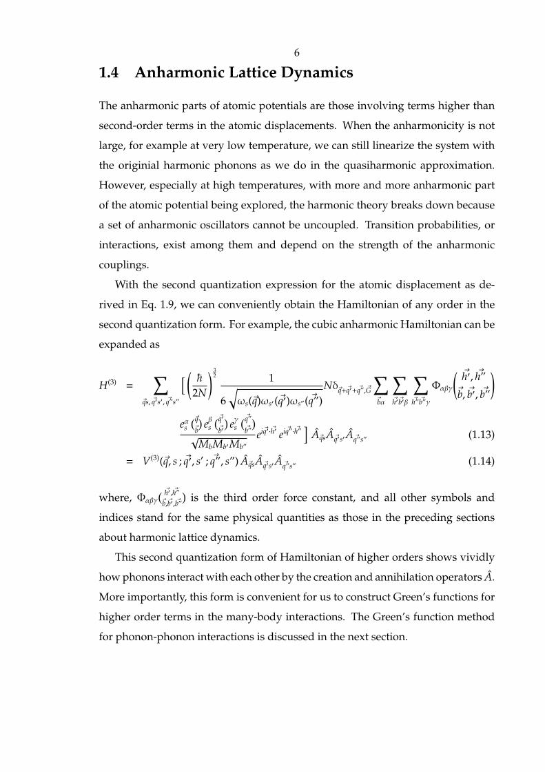
1.4 Anharmonic Lattice Dynamics
The anharmonic parts of atomic potentials are those involving terms higher than
second-order terms in the atomic displacements. When the anharmonicity is not
large, for example at very low temperature, we can still linearize the system with
the originial harmonic phonons as we do in the quasiharmonic approximation.
However, especially at high temperatures, with more and more anharmonic part
of the atomic potential being explored, the harmonic theory breaks down because
a set of anharmonic oscillators cannot be uncoupled. Transition probabilities, or
interactions, exist among them and depend on the strength of the anharmonic
couplings.
With the second quantization expression for the atomic displacement as de-
rived in Eq. 1.9, we can conveniently obtain the Hamiltonian of any order in the
second quantization form. For example, the cubic anharmonic Hamiltonian can be
expanded as
H(3) =∑
qs, q′s′, q”s”
[ ( ~2N
) 32 1
6√ωs(q)ωs′(q′)ωs”(q”)
Nδq+q′+q”,G
∑bα
∑h′b′β
∑h”b”γ
Φαβγ
(h′, h”
b, b′, b”
)
eαs(q
b
)eβs
(q′
b′)
eγs(q”
b”
)√
MbMb′Mb”eiq′·h′ eiq”·h”
]AqsAq′s′Aq”s” (1.13)
= V(3)(q, s ; q′, s′ ; q”, s”) AqsAq′s′Aq”s” (1.14)
where, Φαβγ( h′,h”
b,b′,b”
)is the third order force constant, and all other symbols and
indices stand for the same physical quantities as those in the preceding sections
about harmonic lattice dynamics.
This second quantization form of Hamiltonian of higher orders shows vividly
how phonons interact with each other by the creation and annihilation operators A.
More importantly, this form is convenient for us to construct Green’s functions for
higher order terms in the many-body interactions. The Green’s function method
for phonon-phonon interactions is discussed in the next section.

7
1.5 Green’s Function Method
Condensed matter physics has evolved from traditional solid state physics that
largely focuses on the effective single particle picture in solids to the description of
many-body interactions and collective phenomena in matter. The understanding
of frequencies and lifetimes of interacting quasi-particles at ground or excited states
is one of the most important and interesting topics, and the anharmonic phonon
lifetime and frequency shift are such examples.
The essential feature is that interactions can only be treated correctly by taking
into account the infinite order of ”weak” perturbations. A systematic mathematical
formulation of the many-body interaction is called the Green’s function method,
which is the fundamental theory of the modern condensed matter physics and
is the primary concept of non-relativistic quantum field theory. Some important
concepts and conclusions will be discussed in this section, and in the next section
we will discuss phonon-phonon interactions using this method. More detailed
presentations of the Green’s function method can be found in [1–3].
1.5.1 The Retarded Green’s Function and Lehmann Representa-
tion
We can define a correlation between two Heisenberg operators A(t) and B(t),
GR(t, t′) = − i~θ(t − t′)⟨[A(t), B(t′)]±⟩ (1.15)
where A(t) = eiHt/~Ae−iHt/~ is an operator in the Heisenberg picture with the full
Hamiltonian H. The symbol ⟨⟩ represents the ensemble average and []± chooses
commutators for Fermions or anticommutators for Bosons. It is called the retarded
Green’s function because it works only in the time regime t > t′. To understand the
Green’s function, we may first notice that
GR(t, t′) = GR(t − t′) = − i~θ(t − t′)⟨[A(t − t′), B]±⟩ (1.16)
8
The Green’s function therefore has the fundamental property of a propagator which
characterizes a propagating process of a state containing one additional particle.
For example, we usually specify A(t) = Ψ(t) and B(t′) = Ψ†(t′) where Ψ and Ψ† are
the field operators for destruction and creation. Then the above definition depicts
a propagator which adds a quasiparticle at time t′ and removes it at time t.
The retarded Green’s function contains all necessary information for a interact-
ing system. By Fourier transforming GR, we can obtain
GR(ω) =1Z
∑n,m
e−βEn⟨n|B|m⟩⟨m|A|n⟩ eβ~ωnm ± 1ω − ωnm + iη
(1.17)
whereωnm = ~−1(En−Em) is the energy difference of two excited states n and m in the
interacting system, and η is a positive infinitesimal. Here an integral representation
for the step function is used:
θ(t − t′) = −∫ ∞
−∞
dω2πi
e−iω(t−t′)
ω + iη(1.18)
Eq. 1.17 is the well-known Lehmann representation. GR(ω) is analytic in the up-
per half plane and the poles in the lower half plane determine the energy spectrum
of excitations of the interacting system. GR(ω) may contain even deeper physical
meaning, in that according to the linear response theory,
∆A = GR(ω) e−iωt+η t (1.19)
This implies that the retarded Green’s function is the amplitude of the system’s
response to the external disturbance ω. The amplitude will reach infinity when the
external disturbance is in resonance with the intrisinc frequency ωnm, and hence
gives mathematical poles. On the other hand, the retarded Green’s function is
naturally related to the thermodynamic observables, due to the fact that in second
quantization thermodynamic observables can be expressed as the product of field
operators, and the Green’s function itself is also defined in this way.
In the similar manner, we can define the so called advanced Green’s function

9
GA(ω) by flipping the poles of GR(ω) with respect to the real axis to the upper
half plane. Combining these two Green’s function GR and GA we can obtain the
real-time Green’s function G(ω) which is analytic all over the complex plane except
the real axis. The Green’s function in real space is hence defined as
G(t, t′) = − i~⟨T [A(t), B(t′)]⟩ (1.20)
where the time ordering operator T orders the operators with the latest time t on the
left and includes an addtional factor -1 for each interchange of Fermion operators.
The functions have a common generating function
Γ(z) =∫ ∞
−∞
dω′
2πρ(ω′)z − ω′ (1.21)
This is easily proved to be true by defining ρ(ω) as the imaginary part of GR(ω), and
this quantity can be identified as the density of states. It is then straightforward to
see that z = ω for G and z = ω ± iη for GR and GA respectively.
1.5.2 Perturbation Theory and Wick’s Theorem For Finite Temper-
atures
All the above discussions are based on one assumption that we have known the
eigenstates and energies of the interacting systems H = H0 + H1, which, however,
is what we are trying to resolve in the first place. Therefore, although the Lehmann
representation of Green’s functions shows its power to derive the relationships of
physical observables and obtain the energy spectrum of excited states, we have
to figure out a way to calculate the Green’s function as defined in the Heisenberg
picture in terms of some functions that are already known. Usually, this is done by
perturbation theory.
For finite temperatures (for the zero temperature condition, a similar but much
simpler calculation can be performed in accordance with the Gell-Mann and Low
theorem), we need to first generalize the real time t in the Heisenberg picture
10
and interaction picture to be a complex or pure imaginary time τ, i.e, Ψ(τ) =
eHτ/~ Ψ e−Hτ/~ and ΨI(τ) = eH0τ/~ Ψ e−H0τ/~. In this manner, we define the temperature
Green’s function
g(τ, τ′) = −⟨Tτ[Ψ(τ) Ψ†(τ′)]⟩ (1.22)
where Tτ is the time ordering operator with respect to τ. The Green’s function
consists of a matrix element of Heisenberg operators. This form is inconvenient for
perturbation theory. It can be shown (with the Gell-Mann and Low theorem) that
this Green’s function can be related to the corresponding (generalized) interaction
picture for the field operators and perturbation Hamiltonian H1 in the following
way
g(τ, τ′) = −⟨∑∞n=0
1(−~)n
1n!
∫ β~
0· · ·
∫ β~
0dτn Tτ[H1(τ1)· · ·H1(τn)ΨI(τ) Ψ†I (τ′)]⟩0
⟨∑∞n=0(−~)−n(n!)−1∫ β~
0· · ·
∫ β~
0dτn Tτ[H1(τ1)· · ·H1(τn)⟩0
(1.23)
where ⟨⟩0 represents the non-interacting H0 ensemble average. That the integral
extends from 0 to β~ is reasonable because of the β~ periodicity of g(τ, τ′), and
this magic periodicity also guarantees the transformation of temperature Green’s
function from the τ domain to the frequency domain, which is quite crucial because
it connects with the real-time Green’s function as we will see soon.
Eq. (1.23) shows that we must evaluate the expectation value of time ordering
Tτ products of creation and destruction operators, like ⟨ABC· · · F⟩0. The straight-
forward approach of classifying all possible contributions is very lengthy. Instead,
we shall rely on Wick’s theorem, which provides a general procedure for this
calculation. The main idea is to define a contraction
A•B• = T[A B] −N[A B] (1.24)
where A, B are field operators in the (generalized) interaction picture. The normal
ordering N represents a different order in which all the annihilation operators are

11
placed to the right of all the creation operators. Thus a T product may be evaluated
by reducing it to the corresponding N product. N product is convenient because its
expectation in the non-interacting ensemble average is mostly zero. For example,
according to the definition of g in Eq. (1.22) and the corresponding interaction
picture, Ψ(τ)•I Ψ†I (τ′)• equals −g0(τ, τ′), the non-interacting temperature Green’s
function or free propagator, which is easy to evaluate. Then Wick’s theorem asserts
that < ABC· · ·F >0 is equal to the sum over all possible fully contracted terms, i.e.,
the exact temperature Green’s function g can be expanded in a series containing
the simple products of g0 and perturbation potential. The complete proof can be
found in Ref. [1]. Due to the β~ periodicity of g(τ, τ′) for each of its argument, for
temperature Green’s function, this expansion can be analyzed in energy space at a
discrete set of points ωn, and ωn = 2nπ/β~ for bosons, or (2n+ 1)π/β~ for fermions,
and the corresponding Fourier transformation is
g(ωn) =∫ β~
0dτ eiωnτ g(τ) (1.25)
We can associate a picture, called a Feynman diagram, with each of the terms in
the series expansion. Conventionally, the Green’s function G or g is denoted by a
bold or double solid line with an arrow. The free propagator g0 is denoted by a solid
line with an arrow while the interaction potential is denoted by a wavy line (or
equivalently, by a vertex). These diagrams appearing in the perturbation analysis
form a convenient way of classifying the terms obtained with Wick’s theorem.
One may begin with a few simple diagrams, then all possible summations of lines
and vertices are constructed based on the geometry (called ”putting flesh on the
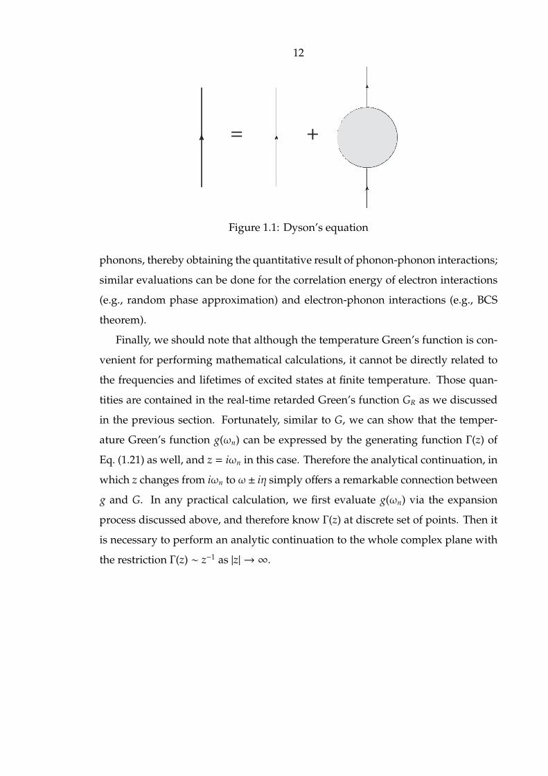
skeletons”). Finally, a particular compact form of this expansion yields Dyson’s
equation
g(ωn) = g0(ωn) + g0(ωn)Σ⋆(ωn)g(ωn) (1.26)
where Σ⋆ is the proper self-energy, in which all the interaction are involved. The
Feynman diagram of Dyson’s equation is shown in Fig. 1.1
In the next section, we will focus on the calculation of the proper self-energy of
12
= +
Figure 1.1: Dyson’s equation
phonons, thereby obtaining the quantitative result of phonon-phonon interactions;
similar evaluations can be done for the correlation energy of electron interactions
(e.g., random phase approximation) and electron-phonon interactions (e.g., BCS
theorem).
Finally, we should note that although the temperature Green’s function is con-
venient for performing mathematical calculations, it cannot be directly related to
the frequencies and lifetimes of excited states at finite temperature. Those quan-
tities are contained in the real-time retarded Green’s function GR as we discussed
in the previous section. Fortunately, similar to G, we can show that the temper-
ature Green’s function g(ωn) can be expressed by the generating function Γ(z) of
Eq. (1.21) as well, and z = iωn in this case. Therefore the analytical continuation, in
which z changes from iωn to ω± iη simply offers a remarkable connection between
g and G. In any practical calculation, we first evaluate g(ωn) via the expansion
process discussed above, and therefore know Γ(z) at discrete set of points. Then it
is necessary to perform an analytic continuation to the whole complex plane with
the restriction Γ(z) ∼ z−1 as |z| → ∞.
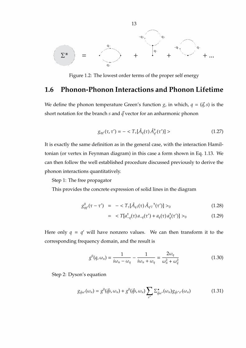
13
= + + + ...Σ*
q 2
q 1
q 2- q 2
q 1
q 1- q1
Figure 1.2: The lowest order terms of the proper self energy
1.6 Phonon-Phonon Interactions and Phonon Lifetime
We define the phonon temperature Green’s function g, in which, q = (q, s) is the
short notation for the branch s and q vector for an anharmonic phonon
gqq′(τ, τ′) = − < Tτ[Aq(τ) A†q′(τ′)] > (1.27)
It is exactly the same definition as in the general case, with the interaction Hamil-
tonian (or vertex in Feynman diagram) in this case a form shown in Eq. 1.13. We
can then follow the well established procedure discussed previously to derive the
phonon interactions quantitatively.
Step 1: The free propagator
This provides the concrete expression of solid lines in the diagram
g0qq′(τ − τ′) = − < Tτ[Aq I(τ) Aq′I
†(τ′)] >0 (1.28)
= < T[a†−q(τ) a−q(τ′) + aq(τ) a†q(τ′)] >0 (1.29)
Here only q = q′ will have nonzero values. We can then transform it to the
corresponding frequency domain, and the result is
g0(q,ωn) =1
iωn − ωq− 1
iωn + ωq=
2ωq
ω2n + ω
2q
(1.30)
Step 2: Dyson’s equation
gqss′(ωn) = g0(qs,ωn) + g0(qs,ωn)∑
s”
Σ⋆qss”(ωn)gqs”s′(ωn) (1.31)

14
We can write the free phonon propagators in Eq. (1.31) in explicit form using
Eq. (1.30) and neglect the non-diagonal terms. We get
gqss(ωn) =2ωs(q)
ω2s (q) + ω2
n − 2ω2s (q)Σ⋆
qss(ωn)
(1.32)
We see the anharmonic Green’s function is of the same form as Eq. (1.30) for the
free propagator in the harmonic approximation. All the effects of anharmonic
interactions are included in Σ⋆. If we write the self energy as a real and imaginary
part, then the frequency shift and lifetime of the phonons are explicitly identified.
Σ⋆qss(ωn) = −∆qss(ωn) + iΓqss(ωn) (1.33)
Step 3: The diagrams of the lowest order terms of the proper self energy are
presented in Fig. 1.2. The mathematical derivation of the 2nd order diagram (the
first diagram on the left) is shown in Appendix A, which is a concrete practice of
the temperature Green’s function approach discussed in this chapter.
The resulting mathematical expressions for these lowest orders diagrams are
∆(3)s (Ω) = −18
~2
∑q1s1
∑q2s2
∣∣∣V(s; q1s1; q2s2)∣∣∣2 × ℘[ n1 + n2 + 1
Ω+ ω1 + ω2− n1 + n2 + 1Ω − ω1 − ω2
+n1 − n2
Ω − ω1 + ω2− n1 − n2
Ω+ ω1 − ω2
](1.34a)
∆(3′)s = −72
~2
∑s1
∑q2,s2
V(s; s; 0s1)V(0s1;−q2s2; q2s2) × ℘( 1ω1
) (n2 +
12
)(1.34b)
∆(4)s =
24~
∑q1,s1
V(s; s; q1s1;−q1s1)(n1 +
12
)(1.34c)
Γ(3)s (Ω) =
18π~2
∑q1s1
∑q2s2
∣∣∣V(s; q1s1; q2s2)∣∣∣2 × [
(n1 + n2 + 1) δ(Ω − ω1 − ω2)
+ 2(n1 − n2) δ(Ω+ ω1 − ω2)]
(1.34d)

15
1.7 Self-Consistent Lattice Dynamics
Consider a crystal with Hamiltonian
H = Tk + V (1.35)
where Tk is the kinetic energy and the potential energy is given by
V =12
∑ll′ψ(rll′ + wll′) (1.36)
Here, rll′ are mean position vectors joining the atoms l and l′, and wll′ are the relative
displacement vectors.
Instead of trying to find the perturbation expansion as we usually do in the
quasiharmonic and anharmonic lattice dynamics, we now consider and effective
harmonic Hamiltonian
H = Tk + V (1.37)
where
V =14
∑ll′
∑αβ
ϕαβ(ll′) wll′αwll′β (1.38)
and the effective force constant ϕ and the mean distance rll′ may be determined
self-consistently.
In essence, this method tries to obtain a mean field of harmonic form and keeps
the field updated. In this process, we want to have the potential difference operator
E = V − V having the eigenvalue ϵ sufficiently small. Under this assumption, the
density matrix operator can be written as
ρ(H) = e−βH = e−β ϵ ρ(H) e−β (E−ϵ) (1.39)
We may disregard the last factor if < e−β (E−ϵ) >H= 1. Here, <>H is the thermal
16
average under the effective Hamiltonian. To the first order, this requires
ϵ =< V >H (1.40)
We can therefore write the free energy approximately as
F = F+ < V >H (1.41)
where
F = −kBT ln Trρ(H) (1.42)
and
< V >H=12
∑ll′< ψ(rll′ + wll′) >H −
14
∑ll′
∑αβ
ϕαβ(ll′) < wll′αwll′β >H (1.43)
Note that< wll′αwll′β >H is the displacement correlation function. Hence, the free
energy can be approximated by the free energy belonging to the effective harmonic
Hamiltonian, and the difference is supposed to be small. Physically speaking, it
means that for a system, even very anharmonic, we may find a harmonic system
that is effectively close enough to the dynamic and thermodynamic properties of
the original one. If this is the case, the problem is greatly simplified because the
harmonic theory is relatively complete.
With modern DFT calculations, several computational algorithms based on the
self-consistent lattice dynamics are being developed. Essentially, these methods
assign large displacements of atoms corresponding to the target temperature by
a random assignment or molecular dynamics simulation, and then try to find the
effective harmonic force constants by optimizing the thermodynamic quantities of
the system [4, 5].
17
Chapter 2
Experimental Methods

18
2.1 Raman Scattering
2.1.1 Introduction
When crystal or molecule is illuminated with monochromatic light of frequency
ωL (usually from a laser in the visible, near infrared, or near ultraviolet range),
it is found that the scattered spectrum of radiation consists of a very strong line
at the frequency of the incident light, as well as of a series of much weaker lines
with frequencies ωL ± ωq, where ωq are found to be equal to some optical phonon
energies. The strong line centered at ωL is known as Rayleigh scattering, which
originates from elastic scattering of photons. The series of weak lines constitute
the Raman sepctrum, which originates from the inelastic scattering of photons by
phonons. The Raman lines at frequencies ωL −ωq are called Stokes lines, and those
at frequenciesωL+ωq are called anti-Stokes lines. The intensities of Stokes lines are
generally much stronger than anti-Stokes lines, and as a result, Raman spectrum is
usually taken on the side of Stokes lines.
Since its discovery, many variations of Raman spectroscopy have been de-
veloped. Examples include surface enhanced Raman, resonance Raman, Raman
microscopy and time-resolved stimulated Raman spectroscopy. Owing to its great
versatality, Raman spectroscopy has been widely used in physics, chemistry, geol-
ogy, biology and many other fields of science and engineering. In chemistry and
geology, for example, Raman spectra are usually used to collect a fingerprint by
which the molecule or crystal can be identified, owing to the fact that vibrational
information is specific to the chemical bonds and symmetry. It also provides a
convenient way to perform in situ or non-destructive measurements, which is ex-
tremely important in many fields. For physicists and materials scientists, it is an
excellent tool for studying excitations such as phonons, magnons and excitons in
solids.
In our work, Raman spectroscopy is mainly used to investigate anharmonic
phonon behavior under temperature, and we will focus on first order Raman

19
scattering. In first order Raman scattering, only optical phonons with momentum
equal to zero are involved, as a consequence of the large momentum difference
between phonons and photons. Although this is a limitation, Raman spectroscopy
probes phonon modes with extremely high resolution in energy, which is of great
value to study the phonon anharmonicity characterized by the energy broadening
and shift, for example.
In this section, we will focus on the theories of Raman scattering. The ex-
perimental details will be discussed, along with the specific descriptions of data
collection, in Chapters 4 to 6, and Appendix C, in which particular samples are
in study. Here, we start with a brief discussion of the classical theory of Raman
scattering. We then introduce the quantum theory to describe quantitatively how
photons interact with phonons in those inelastic scattering processes. We then
spend considerable efforts deriving and discussing Raman selection rule. The se-
lection rule is established with quantum theory and group theory; it provides the
fundamental information of symmetries of modes, and is therefore critical for our
study in understanding phonon dynamics.
2.1.2 The Frequency Resolved Raman Spectroscopy
2.1.2.1 Classical Theory
Let E = E0 cosωLt be the electric field vector of the incident light and Q be the
normal coordinate of small displacements of the nuclei, the dipole moment M is
contributed by two parts,
M = Md(Q) + α(Q)E (2.1)
where Md(Q) is the static dipole moment of the system plus the response to the
atomic displacements. When the incident light is in the infrared, the atomic dis-
placement is the dominant mechanism for scattering light, and the moment Md(Q)
drives the infrared scattering. On the other hand, the Raman effect originates with
the electric field induced dipole moment Me = α(Q)E. Here α(Q) is the polarizabil-

20
ity, in general, Me does not coincide with the direction of E, and the polarizability
is thus a second-order tensor. It can be shown further that it is symmetrical, i.e.,
αT = α, hence only six of the nine components of α are independent.
Expanding the static dipole moment, Md(Q), and the polarizability, α(Q), in
terms of Q, we obtain
M = Md0 +
∂Md
∂Q
0
Q + α0E +(∂α∂Q
)0
QE +O(Q2) (2.2)
In the following discussion of the fundamental principles, we will mainly focus
on the Raman effect since the mathematical treatment of infrared scattering is
similar. We drop the subscript e of Me for brevity.
If a molecule vibrates with the frequency ωq, we have Q = Q0 cosωqt and the
electric field induced dipole moment can be written
M(t) = α0E0 cosωLt +12
(∂α∂Q
)0
Q0E0[cos(ωL − ωq)t + cos(ωL + ωq)t] (2.3)
According to the rule of electromagnetic radiation, the intensity of radiation
emitted by the dipole moment Me(t) into the solid angle dΩ = sinθ dθ dϕ is given
by
dI(t) =dΩ
4πc3 sin2 θ | ¨M(t)|2 (2.4)
Hence, the intensity of the scattered light per unit sold angle is give by
I(t) = E20 α
20ω
4L cos2ωLt +
14
E20
(∂α∂Q
)2
0
Q20 [(ωL − ωq)4 cos2(ωL − ωq)t (2.5)
+ (ωL + ωq)4 cos2(ωL + ωq)t]
It follows that the ratio of the intensities of the Stokes and anti-Stokes lines
should beIS
IAS=
(ωL − ωq)4
(ωL + ωq)4 (2.6)
This is less than unity, which is found to be contrary to the experimental observa-

21
tion. This inconsistency is eliminated in the quantum theory of the Raman effect,
as discussed next.
2.1.2.2 Quantum Theory and Placzek’s Approximation
The fundamental problem of the classical treatment is that we ignore the quantum
character of electrons and phonons, and we do not consider the occupancy factor
in those quantum states. Consider a system (crystal or molecule) with Hamiltonian
H obeying the time dependent Schrodinger equation
H0ψ(0)(t) = i~
∂∂tψ(0)(t) (2.7)
and the general solution is a superposition of the eigenfunctions ϕr’s of the time
independent Schrodinger equation (where ϕr = (e,n) denotes collectively the elec-
tronic quantum numbers e and the vibrational quantum numbers n.)
ψ(0)(t) =∑
r
crϕre−iωrt (2.8)
Suppose that this system is perturbed by a light wave with the electric field
vector E = E0e−iωLt. The Schrodinger equation of the perturbed system is
(H0 − E · M)ψ(t) = i~∂∂tψ(t) (2.9)
Qualitatively speaking, the wave functions of the perturbed system acquires a
mixed character of all possible wave functions of the unperturbed system. We can
regard it as a non-stationary state only for a physical description of this perturbation
process, a so called ”virtual state” in Raman scattering.
Rigorously, if the unperturbed system is in the stateϕk, using the time-dependent
perturbation theory, it can be easily shown that the first order perturbed state is
ψ(1)k =
1~
∑j
E0 · Mkj
ω jk − ωLϕ j
exp[−i (ωk + ωL)t] +1~
∑j
E0∗ · Mkj
ω jk + ωLϕ j
exp[−i (ωk − ωL)t]
(2.10)

22
where Mkj =< ϕk|M|ϕ j > and ω jk = ωk − ω j. Meanwhile, the matrix element of the
dipole moment of the perturbed system is
M(p)km(t) = < ψ∗m |M|ψk > (2.11)
= Mkm exp(−iωkmt) + Ckm exp[−i (ωkm + ωL)t] + Dkm exp[−i (ωkm − ωL)t]
where
Ckm =1~
∑j
(E0 · Mkj)M jm
ω jk − ωL+
Mkj(E0 · M jm)ω jm + ωL
(2.12)
Dkm =1~
∑j
(E0∗ · Mkj)M jm
ω jk + ωL+
Mkj(E0∗ · M jm)ω jm − ωL
(2.13)
According to Eq. 2.4, we can obtain the intensity of the radiation by the dipole
moment M(p)km(t).
Ikm =4
3c3 [ω4km |Mkm|2 + (ωkm + ωL)4 |Ckm|2 + (ωkm − ωL)4 |Dkm|2] (2.14)
Using Eq. 2.12, the components of Ckm can be written in the form
(Cµ)km =∑ν
(cµν)kmE0ν (2.15)
where the scattering tensor
(cµν)km =1~
∑j
(Mν)kj (Mµ) jm
ω jk − ωL+
(Mµ)kj (Mν) jm
ω jk + ωL(2.16)
If the incident light is polarized in the direction of µ and the scattered light is
observed with the analyzer in the direction of ν, one finds for the scattered radiation
emitted per unit solid angle dΩ
Ikm[µν] =1c4 (ωkm + ωL)4 |(cµν)km|4 I0 (2.17)
23
The direct evaluation of the scattering tensor (cµν)km is not practical in molecules
and crystals due to the complexity of the energy levels and the incomplete knowl-
edge of the excited states j’s. However, the scattering tensor of Eq. 2.16 derived by
the quantum theory does provide a direct way determining the Raman-activity in
terms of group symmetry.
Using Placzek’s approximation, it is possible to obtain the general result about
the direct relationship between the Raman scattering tensor and the electronic
polarizability. The physical idea of this approximation is quite straightforward.
Since in most cases of Raman scattering, ωeo > ωL >> ωnn′ , i.e., the exciting laser
frequency is less than any electronic transition frequency of the system, although
much larger than any vibrational frequency. In this sense, only the electrons but
not the atoms can respond to the light field. Therefore, only the electronic part of
the wavefunction is modified by the incident light and is the same for each atomic
configuration, denoted by r, as for the system with fixed nuclei. Hence the Raman
scattering tensor is equal to the electronic polarizability tensor
(cµν)0n,0n′ =
∫ψ∗0n′(r)[cµν(r)]00ψ0n(r) dr = (αµν)0n,0n′ (2.18)
whereψ0n(r) is the vibrational part of wave function of configuration r and [cµν(r)]00
is the scattering tensor of the electronic ground state, which is identical with the
electronic polarizability. This establishes the fundamentals of Raman selection
rules; and more recently, the calculation of Raman intensity using first principles
mostly relies on this approximation.
By using the same treatment as in the classical approach,
(αµν)nn′ = (αµν)0δnn′ +
(∂αµν∂Q
)0
Qnn′ (2.19)
24
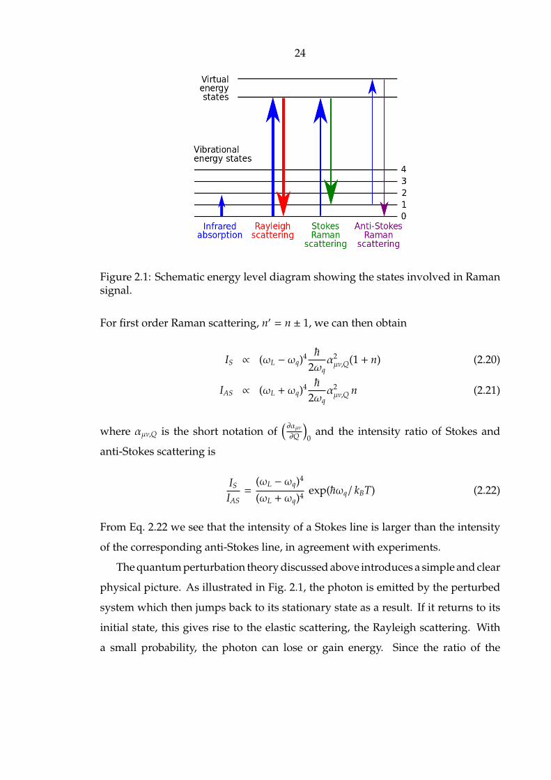
Figure 2.1: Schematic energy level diagram showing the states involved in Ramansignal.
For first order Raman scattering, n′ = n ± 1, we can then obtain
IS ∝ (ωL − ωq)4 ~
2ωqα2µν,Q(1 + n) (2.20)
IAS ∝ (ωL + ωq)4 ~
2ωqα2µν,Q n (2.21)
where αµν,Q is the short notation of(∂αµν∂Q
)0
and the intensity ratio of Stokes and
anti-Stokes scattering is
IS
IAS=
(ωL − ωq)4
(ωL + ωq)4 exp(~ωq/ kBT) (2.22)
From Eq. 2.22 we see that the intensity of a Stokes line is larger than the intensity
of the corresponding anti-Stokes line, in agreement with experiments.
The quantum perturbation theory discussed above introduces a simple and clear
physical picture. As illustrated in Fig. 2.1, the photon is emitted by the perturbed
system which then jumps back to its stationary state as a result. If it returns to its
initial state, this gives rise to the elastic scattering, the Rayleigh scattering. With
a small probability, the photon can lose or gain energy. Since the ratio of the
25
populations of two stationary states is proportional to exp(~ωq)/kBT, the ratio of
the intensities of a Stokes line to a corresponding anti-Stokes line is expected to be
proportional to Eq. 2.22.
It should be emphasized that, the Raman scattering of light is due to the electrons
of the system, and as shown in the next section, the transfer of the energy between
the light and nuclei is only possible through the coupling of electrons and nuclei.
It can be shown that there is no Raman scattering for a pure harmonic oscillator
with frequency ω0. In this case, the evaluation of dipole moment matrix Mkm only
involves the phonons but not the electrons, and can be simply written as
(Mµ)nn′ = e (~
2mω0)
12 [(n + 1)
12δn,n′+1 + n′
12δn,n′−1] (2.23)
It follows that the terms of Eq. 2.16 cancel off and hence the Raman scattering
tensor (c)n,n±1 vanishes. It should be mentioned that Raman scattering exists for an
anharmonic oscillator, however this does not mean that Raman scattering is due
to anharmonic motion of the nuclei. This is only the case for the radiation which
originates with the scattering from the nuclei themselves, known as the ionic Raman
effect. The essential part of the normal Raman scattering by molecules and crystals,
however, comes from the scattering by the electrons as presented in Eq. (2.18),
and the energy transfer between the light and the motion of nuclei provides the
important information of harmonicity and anharmonicity of phonons.
2.1.2.3 Loudon’s Third Order Perturbation Theory
Loudon’s approach explicitly assesses the scattering process of electrons, phonons
and the light wave by the third-order time-dependent perturbation theory, which
is theoretically equivalent to the discussion of the preceding section but more
direct. [6] As proposed by Loudon, the Raman process is described by a three-step
scattering process, involving three virtual electronic transitions accompanied by the
energy transfer of photons and phonons. Therefore, the transition probability of
the system from the state with ni incident photons, 0 scattered photon, nq phonons

26
and electron ground state (denoted by 0) to the final state with one new scattered
photon and one new phonon is
W(t) =∑q, ks
∣∣∣< ni − 1, ns + 1; nq + 1; 0 | e−iHt/~ | ni,ns; nq; 0 >∣∣∣2 (2.24)
=2πt~6
∑q, ks
∣∣∣∣∣∣∣∑m,n < ni − 1,ns = 1; nq + 1; 0|H|m >< m|H|n >< n|H|ni, ns = 0; nq; 0 >(ωm − ωi)(ωn − ωi)
∣∣∣∣∣∣∣2
×δ(ωi − ωq − ωs)
where H = HER + HEP, the total Hamiltonian of electron–photon (radiation) and
electron–phonon interactions. Followed by Eq. 2.24, the scattering ratio is
Ns
Ni∝ (nq + 1)
ωs
ωi
∣∣∣Rqi,s(−ωi,ωs,ωq)
∣∣∣2 (2.25)
where
Rqi,s(−ωi,ωs,ωq) =
1V
∑m,n
(Ms)0n(Θq)nm(Mi)m0
(ωn + ωq − ωi)(ωm − ωi)+ f ive similar terms
(2.26)
here the scripts of Rqi,s stand for the polarization directions of the incident and
scattered photons i and s, and the phonon q. The two matrix elements M arise
from the electron-photon Hamitonia HER and Θ arises from the electron-phonon
Hamiltonia HEP. Loudon’s formula is important to define some complex selection
rules in the resonant Raman scattering. For example, in the case of the exciton-
assisted Raman scattering on Cu2O, the electric quadupole and magnetic dipole
transition has to be considered, and one HER term in Eq. 2.26 can be used to represent
this symmetry [7, 8].
27
2.1.3 Group Theory and Selection Rules
2.1.3.1 Classical Approach
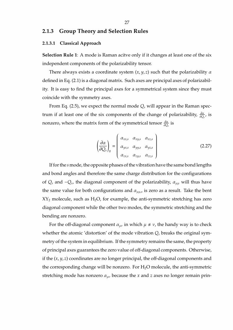
Selection Rule 1: A mode is Raman acitve only if it changes at least one of the six
independent components of the polarizability tensor.
There always exists a coordinate system (x, y, z) such that the polarizability α
defined in Eq. (2.1) is a diagonal matrix. Such axes are principal axes of polarizabil-
ity. It is easy to find the principal axes for a symmetrical system since they must
coincide with the symmetry axes.
From Eq. (2.5), we expect the normal mode Qs will appear in the Raman spec-
trum if at least one of the six components of the change of polarizability, ∂α∂Qs
, is
nonzero, where the matrix form of the symmetrical tensor ∂α∂Qs
is
(∂α∂Qs
)0
=
αxx,s αxy,s αxz,s
αyx,s αyy,s αyz,s
αzx,s αzy,s αzz,s
(2.27)
If for the s mode, the opposite phases of the vibration have the same bond lengths
and bond angles and therefore the same charge distribution for the configurations
of Qs and −Qs, the diagonal component of the polarizability, αµµ will thus have
the same value for both configurations and αµµ,s is zero as a result. Take the bent
XY2 molecule, such as H2O, for example, the anti-symmetric stretching has zero
diagonal component while the other two modes, the symmetric stretching and the
bending are nonzero.
For the off-diagonal component αµν in which µ , ν, the handy way is to check
whether the atomic ’distortion’ of the mode vibration Qs breaks the original sym-
metry of the system in equilibrium. If the symmetry remains the same, the property
of principal axes guarantees the zero value of off-diagonal components. Otherwise,
if the (x, y, z) coordinates are no longer principal, the off-diagonal components and
the corresponding change will be nonzero. For H2O molecule, the anti-symmetric
stretching mode has nonzero αµν because the x and z axes no longer remain prin-

28
cipal axes during the vibration of this mode, while the other two modes are zero.
Therefore, all three modes in H2O are Raman-active.
This method is simple and practical, however, for complex crystal structures,
this rule is extremely difficult to apply. In the next subsection, we introduce a
rigorous and systematic approach to find the selection rule,which is based on the
group representation theory in quantum mechanics.
2.1.3.2 Group Theoretical Approach
Selection Rule 2: A mode s is Raman active only if the normal coordinate Qs
transforms in the same way as one of the polarizability components αµν.
Let’s first present an argument that is rigorous but impractical. The intensity of
the scattered light is given by Eq. (2.17), in which the component of the polarizability
is explicitly calculated using Eq. (2.18). In quantum mechanics, group theory can
greatly help to judge whether a given matrix element vanishes by symmetry, and
in our case, the assessment of the polarizability matrix leads to the Raman selection
rule. From the integral of Eq. (2.17) and unitarity of the symmetry operation group
R,
< n′ |αµν| n > =
∫ψ∗0n′(r)[αµν(r)]00ψ0n(r) dr (2.28)
=1g
∑R
< Rψ0m | RαµνR−1 | Rψ0l >
=∑
m′, l′, µ′, ν′< m′ |αµ′ν′ | l′ >
1g
∑R
Dmm′D(α)µ′ν′Dll′ (2.29)
where D’s are the matrix representations of the symmetry group R with basis
functions as state vectors ψl, where Rψl =∑ψl′Dl′l or tensor elements αµν, where
RαµνR−1 =∑αµ′ν′ D
(α)µ′ν′ . Due to the orthogonality relation of different basis func-
tions, a possible vibrational transition |n > to |n′ > is nonzero, or Raman active, if
and only if the representation D(α) of one or more of the polarizability component
29
occurs in the reduction of D(vib,2) ×D(vib,2), where the components of the polarizabil-
ity tensor transform like the vector operators x2, y2, z2, xy, yz, zx since these tensor
elements have the form of dipole × dipole, as can be seen from Eq. (2.16). This rule
is quite general, however, we have to first work out the irreducible representations
of all the vibrational states and then test all possible pairs of states to see whether
the transition between them is allowed. Moreover, this rule does not consider the
energy difference and the order of intensity, i.e., which lines are the strong ones.
Here is a more practical approach. In accordance with Eq. (2.19), we can at
least have three important conclusions for first order Raman scattering: (1) the
symmetry of(∂αµν∂Qs
)0
Qs is just the symmetry of the normal mode Qs because the
derivative part is a scalar. (2) This term must always have the same symmetry of
αµν itself. (3) the Raman spectrum contains the fundamental line of frequency shift
ωs. Hence, we finally obtain the selection rule summarized on top of this section.
The selection rule for infrared scattering is completely analogous, in which we can
expand the dipole components in the same way. As a result, the determination
of Raman-activity is reduced to testing the existence of the normal modes that
transform in the same way as x2, y2, z2, xy, yz or zx.
Further, since the Hamiltonian H and the symmetry operations R commute,
any group member of symmetry operations cannot transform one mode to another
with a different dynamic eigenvalue, i.e., under the irreducible representations of
H, and the H matrix is diagonal, the matrix of R must be blocks of irreducible
representations of the symmetry group, and the rank of each block equals to the
degeneracy of the corresponding normal mode. The physical idea for this irre-
ducibility in lattice vibration is a normal mode coordinate Qs is decoupled from
other normal coordinates. As a result, the displacement pattern of a normal mode
is invariant under the symmetry operation and hence RQs must have the same
frequency. One simple illustration of the matrix representations of H and R under
the eigenbasis of H, with one doubly degenerate and two single modes, is

30
H =
λ1 0 0 0
0 λ1 0 0
0 0 λ2 0
0 0 0 λ3
⇐⇒ R =
× × 0 0
× × 0 0
0 0 × 0
0 0 0 ×
(2.30)
Accordingly, we can group the modes in accordance with the irreducible rep-
resentation of the symmetry of molecules or crystals. More explicitly, since H and
R own the same eigenbasis, we can fully understand the symmetry of modes by
means of R, instead of H itself.
Combining the arguments discussed above, we obtain the following math-
ematical statement about how to apply the Rule 2: we need to transform the
corresponding symmetry group to a sum of irreducible representations (in a form
that looks like the above illustrative example), and the modes belonging to the
representations that inherit the symmetry of vector products x2, y2, z2, xy, yz, zx are
expected to be Raman active.
2.1.3.3 The Correlation Method
Although the rule derived from group theory is mathematically handy, the irre-
ducible decomposition is still nontrivial, and sometimes complicated. The cor-
relation method that relates the site symmetry of a system to the corresponding
crystallographic point symmetry offers a convenient way generating the selection
rule. In this section, we follow the approach described by Inui et al. [9]
To understand this method, we need some definitions and fundamental theo-
ries.
Site Group S: The site is defined as a point which is left invariant by some
operations of the space group. These operations may be shown to form a group
which is called the site group. Every point is thus a site, having at least the trivial
site group C1.
Point Group G0: For a space group G, rotational parts of the symmetry opera-
tions will form a group G0, which is a crystallographic point group. Evidently, S is
31
a subgroup of G0.
Factor Group G/T: The translation group T forms an invariant subgroup of the
space group G. Therefore, the cosets of the translation group T in the space group
G form a factor group G/T, and it is isomorphic to the point group G0, though some
of the cosets may contain other than pure point operations combined with screws
or glides.
This is indeed the group theoretical counterpart of the Bloch theorem, in which,
the Bloch functions are actually the basis functions for the irreducible representation
of T and inherit all the translational symmetry of the crystal. The wavevector k
designates the representation of the translation group with the character exp(ik · r ).
At Γ point, the G0 symmetry is maintained for the obvious reason, in consequence,
for 1st order Raman scattering, the G0 symmetry determines the activity of spectra.
However, it should be noted that k generally cannot have the whole symmetry of
G0 but constitutes a subgroup, this explains the change of Raman activity when
going to higher order Raman scattering in which k is not at the Γ point, for example,
overtone or combinational bands in Raman.
Since the normal coordinates are linear combinations of the 3N atomic displace-
ments, the correlation method starts with the irreducible representation of the site
group S, and tries to transform to the point group symmetry of the system. Ob-
viously, under the site group’s operation, one atom will never be moved away to
another position, the ’mutual exclusion’ implies that the bases for the irreducible
representations are simply composed of the xyz coordinates (or displacements) of
each individual atom, with no superposition of other atoms. Therefore, the irre-
ducible representations of the site group are easily identified by picking out those
representations with Tx, Ty or Tz symmetry, which are followed by the basis vectors
x, y and z. Then, we can relate the site representation to the factor representation by
examining the character χ (the trace of the group representation). Under the trans-
formation between these two representations, the trace of the matrix is a constant.
As a result, the character of ith irreducible representation of the factor group is just
the same as that of the site group, or the sum of several irreducible representations

32
of the site group (because the symmetry of factor group is higher, the degeneracy
of the factor group can be lifted), i.e.,
χ(β)f (R) =
∑(α)
aβα χαs (R) (2.31)
where s and f stand for site and factor respectively. This provides a straightforward
way to construct the correlation between two groups by comparing the character
tables.
When irreducible matrices of a representation is derived, we can define a pro-
jection operator
P(β) f =dβg
∑R
χ(β)(R)∗ R (2.32)
Consider an arbitrary function f , it will contain in gereral, basis functions of various
irreducible representations
f =∑β
∑m
c(β)m ϕ
(β)m (2.33)
where ϕ(β)m are basis functions for the irreducible representation D(β), and c(β)
m are
coefficients of the expansion. For the vibration spectra, ϕ(β)m ’s are the normal coor-
dinates Q’s for the mode β.
When applied to f , P(β) will project f onto the subspace of the representation
D(β).
P(β) f =∑
m
c(β)m ϕ(β)
m (2.34)
In practice, for the Raman spectra, we can take f as the displacement of one atom.
Examples of the rutile and cuprite structures are presented in Appendix B. More
examples can be found in the manual book written by Fateley et al. [10]

33
2.2 Time of Flight Inelastic Neutron Scattering
2.2.1 Introduction
Neutron scattering is a powerful technique for studying lattice dynamics. One
advantage stems from the fact that the wavelength of a neutron is of the same
order of magnitude as the interatomic distances in crystals. Therefore, it has good
resolution in reciprocal space and is able to probe phonons in the whole Brillouin
zone. A historical disadvantage of neutron scattering is the relatively poor energy
resolution, due to the low intensity of available neutron beams. This situation has
changed with low background and high neutron flux at the Spallation Neutron
Source (SNS) at the Oak Ridge National Laboratory.
In our work, inelastic neutron scattering is used to investigate the phonon
densities of states. The measurements were performed with the wide angular-
range chopper spectrometer (ARCS) at SNS at the Oak Ridge National Laboratory.
In this section, we briefly review the basic principles and experimental techniques
of inelastic neutron scattering and its applications in the study of lattice dynamics.
More detailed discussions about theories of inelastic neutron scattering can be
found, for example, in [11, 12].
2.2.2 Basic Principles
2.2.2.1 Scattering Cross Section
When a beam of monoenergetic thermal neutrons is incident on a sample, the
neutrons may be either scattered, absorbed or pass with no interaction. The process
of neutron scattering is characterized by the cross section σ. The scattered intensity
is usually described by the partial differential cross section, which is defined to be
d2σ
dΩdE=
number o f neutrons scattered per second into solid angle dΩwith energy Eincident neutron f lux
(2.35)
The strength of the a neutron-nucleus interaction is described by the scattering
34
length b, which in general is a complex quantity ( the imaginary part gives the
neutron absorption). Since nuclear forces are short in range compared to the
neutron wavelength, in the first order Born approximation the interaction potential
between the neutron and the nucleus at R can be approximated by the Fermi
pseudopotential
V(r ) =2π~2b
mδ(r − R ) (2.36)
The cross section is evaluated in the Born approximation. The incoming neu-
trons are represented by plane wave functions, and the transition probability is
given by Fermi Golden rule, together with the Fermi pseudopotential, we can
obtain
d2σ
dΩdE=
k f
ki
12π~
∑l,l′
blbl′ ×∫ ∞
−∞⟨exp[−iQ · Rl′(0)] exp[iQ · Rl(t)]⟩ exp(−iωt)dt (2.37)
where Q = ki − k f is the momentum transfer to the sample, and ω = (Ei − E f )/~ is
the energy transfer to the sample.
2.2.2.2 Coherent and Incoherent Scattering
The cross section in Eq. 2.37 contains products of pairs of scattering lengths, which
can be written as the sum of a correlated part and an uncorrelated part
blbl′ = |b|2 + δll′(b2 − |b|2) (2.38)
The coherent scattering is proportional to the average value b, and incoherent
scattering arises from the distribution of the deviations from b. Only a system with
an average scattering length can give interference effects.
As a result, the cross section can be split in a coherent part(d2σ
dΩdE
)coh= b
2 k f
ki
∑l,l′
∫ ∞
−∞⟨exp[−iQ · Rl′(0)] exp[iQ · Rl(t)]⟩ exp(−iωt)dt (2.39)
35
and an incoherent part(d2σ
dΩdE
)inc= (b2 − b
2)
k f
ki
∑l
∫ ∞
−∞⟨exp[−iQ · Rl(0)] exp[iQ · Rl(t)]⟩ exp(−iωt)dt (2.40)
These equations show that coherent scattering depends on the correlations between
different scatterers at different times, while the incoherent scattering involves only
the correlations between the positions of the same scatterer at different times. The
coherent and incoherent scattering for different elements can be quite different.
For example, the scattering is mostly coherent for vanadium-50 but incoherent for
vanadium-51.
Consider a crystal as a target for the thermal neutron beam. The position of a
nucleus at time t is given by Rl = rl+ ul (t), in which rl is the equilibrium position of
the atom in the Bravais lattice, and ul (t) is the displacement. Insert the expression
for Rl into Eq. 2.39 and notice that the correlation between atoms at rl and rl′ in a
Bravais lattice depends only on rl − rl′ , we get(d2σ
dΩdE
)coh= b
2 k f
ki
∑l
exp(iQ · rl) ×∫ ∞
−∞⟨exp[−iQ · u0(0)] exp[iQ · ul(t)]⟩ exp(−iωt)dt
(2.41)
Expressing the displacements rl in the second quantization form as derived in
Eq. 1.9, one can show that [11]
⟨exp[−iQ · u0(0)] exp[iQ · ul(t)]⟩ = exp[⟨Q2u20(0)⟩] exp[⟨Q · u0(0) Q · ul(t)⟩] (2.42)
where the first factor exp[⟨Q2u20(0)⟩] corresponds to the Debye-Waller factor, exp(−2W).
The partial cross section of Eq. 2.41 can be rewritten as(d2σ
dΩdE
)coh= b
2 k f
kie−2W
∑l
exp(iQ·rl)×∫ ∞
−∞exp[⟨Q·u0(0) Q·ul(t)⟩] exp(−iωt)dt (2.43)
If we expand the second exponential factor of Eq. 2.42 in a Taylor series, Eq. 2.43
has a quite clear physical meaning. It just gives the multi-phonon expansion

36
which describes zero, first, second...order processes. The zero-th term corresponds
to elastic scattering, the first-order term corresponds to the one-phonon process,
the second-order term corresponds to the two-phonon process and so on. The
coherent one-phonon scattering process can be considered as elastic scattering on
a moving target crystal, while higher-order processes give a broad distribution in
the momentum and energy space and can be considered as the background [11].
The evaluation of the incoherent scattering, Eq. 2.40, is similar. The exponent
can be expanded in a power series, and the nth term corresponds to the n-phonon
process. As compared to the coherent cross section, there is only the energy con-
servation factor, therefore, the measurement of the incoherent scattering provides
information only on the number of phonon modes as a function of energy but not
on the dispersion relations.
2.2.3 Wide Angular-Range Chopper Spectrometer (ARCS)
Thermal neutrons can be produced in a nuclear reactor by a chain reaction of
nuclear fission or by spallation reactions with heavy metals. An important experi-
mental work on Ag2O presented in this thesis made use of time-of-flight inelastic
neutron scattering (INS) performed with the Wide Angular-Range Chopper Spec-
trometer (ARCS) at the Spallation Neutron Source (SNS) at the Oak Ridge National
Laboratory [13]. The source of the neutrons is the spallation of neutrons from a
mercury target bombarded with high energy protons. The SNS is currently the
most powerful neutron source in the world.
The initial energies of the neutrons are too high for materials science research,
and they are slowed down by passing through cells filled with water. The pulsed
neutron beam is then directed to the instrument through neutron guides, inside of
which the neutrons undergo total reflection, so the loss of intensity is negligible.
Two choppers rotating with different frequencies allow selection of the incident
energy E0 of neutrons. The first chopper is more massive and stops high energy
neutrons and other background radiation. The second chopper, usually called a
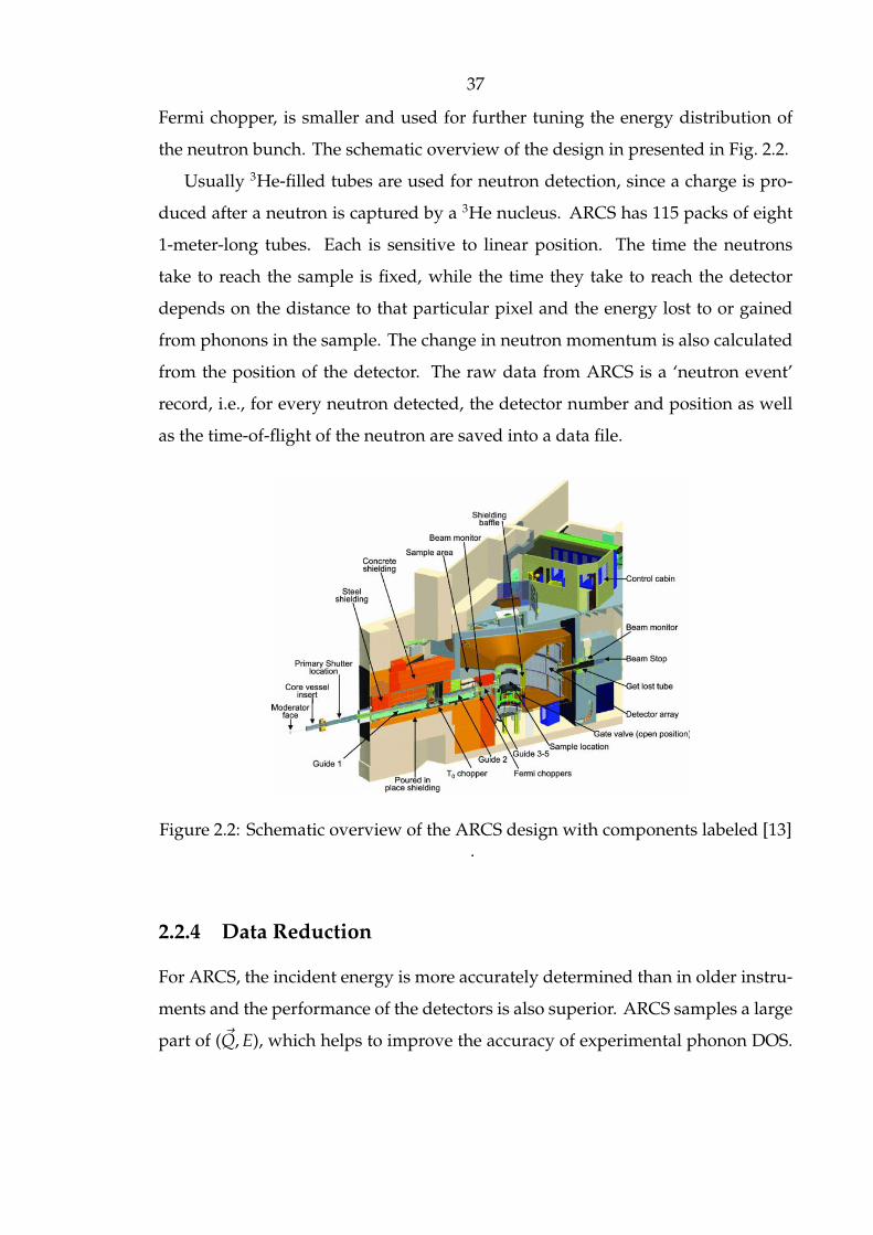
37
Fermi chopper, is smaller and used for further tuning the energy distribution of
the neutron bunch. The schematic overview of the design in presented in Fig. 2.2.
Usually 3He-filled tubes are used for neutron detection, since a charge is pro-
duced after a neutron is captured by a 3He nucleus. ARCS has 115 packs of eight
1-meter-long tubes. Each is sensitive to linear position. The time the neutrons
take to reach the sample is fixed, while the time they take to reach the detector
depends on the distance to that particular pixel and the energy lost to or gained
from phonons in the sample. The change in neutron momentum is also calculated
from the position of the detector. The raw data from ARCS is a ‘neutron event’
record, i.e., for every neutron detected, the detector number and position as well
as the time-of-flight of the neutron are saved into a data file.
Figure 2.2: Schematic overview of the ARCS design with components labeled [13].
2.2.4 Data Reduction
For ARCS, the incident energy is more accurately determined than in older instru-
ments and the performance of the detectors is also superior. ARCS samples a large
part of (Q,E), which helps to improve the accuracy of experimental phonon DOS.
38
However, the data reduction of inelastic neutron scattering is still a complicated
task, not only due to the difficulty of binning a large amount of data, but also due
to the complexity of multiphonon and multiple scattering corrections. The detailed
principles and procedures are documented elsewhere [12–14], and the develope-
ment of the corresponding software package was an important part of the DANSE
project [15]. Here, we give a brief overview about the data reduction procedures
for ARCS.
The raw data are processed to obtain I(Q,E) histograms. The binning of the
energy transfer and the momentum transfer are the main variable at this stage, and
there is a trade-off between the two axis in terms of counting statistics. The binning
used for the present work, 0.5 meV per energy bin and 0.1 Å per momentum bin,
is fairly standard.
The background subtraction is performed next. A measurement under the same
experimental conditions and sample environment is done, but without the sample.
This accounts for most of the real contribution from the background. At ARCS
the instrument background is quite low because it is almost completely shielded
by neutron-absorbing materials, including in between detector packs. Most of the
background comes from the sample environment.
Neutron-weighted phonon DOS curves are obtained from the I(Q,E) histograms,
using getDOS, part of the DANSE software. For incoherent scatterers of neutrons,
the phonon DOS is obtained by integrating over the Q axis. The subtraction of
the elastic scattering is done by assuming an E2 scaling of the intensity of the
phonon DOS and fitting the elastic peak to a Gaussian. The main issue that the
code deals with is the determination and subtraction of multiphonon scattering,
which is solved by an iterative method: the n-phonon scattering can be written as
the convolution of the 1- and (n-1) -phonon scattering and this leads to a recursion
relation for all the orders of scattering, with one adjustable parameter. A detailed
description of the getDOS and underlying principles is given in [12, 14]

39
Chapter 3
Computational Methodologies
40
3.1 Density Functional Theory
3.1.1 Introduction
The fundamental principle of density function theory (DFT) is that any property
of a system of many-body interactions can be viewed as a functional of the ground
state density, which, in principle determines all the information for the ground
state. The existence proof was given by Hohenberg and Kohn [16]. Kohn and Sham
then provided an approach to make ground state functionals for real systems of
many electrons [17]. The remarkable successes of the functionals of local density
approximation (LDA) and generalized gradient approximation (GGA) within the
Kohn-Sham approach lead to widespread interests and applications in DFT. Here,
we briefly review the DFT theory. More theoretical details on this subject can be
found in [18].
3.1.2 Hohenberg-Kohn Theorems
For a system of electrons and nuclei in an external potential Vext(r ), the Hamiltonian
can be written
H = − ~2
2me
∑i
∇2i +
∑i
Vext(r ) +12
∑i, j
e2
|ri − r j |+ Hnn (3.1)
where Vext(r ) includes interactions of electrons and nuclei and any other external
fields, and Hnn is nuclei-nuclei interaction potential.
The first theorem states that for this system, the potential Vext(r ) is determined
uniquely, except for a constant, by the ground state electron density n0(r ). Since
the Hamiltonian is fully determined, it follows that all properties of the system are
completely determined given only the ground state density.
The second theorem states that given the external potential there exists a unique
energy functional E[n(r )], and the exact ground state energy of the system is the
global minimum value of this functional, and the density n(r ) that minimizes the
41
functional is the exact ground state density n0(r ).
According to the first theorem, the ground state energy functional can be written
in the form
E[n(r )] = T[n(r )] + Eint[n(r )] +∫
d3rVext(r )n(r ) + Enn (3.2)
= FHK[n(r )] +∫
d3rVext(r )n(r ) + Enn (3.3)
where the functional FHK[n(r )] includes kinetic and potential energies of the inter-
acting electron system. It follows from the second theorem that if the functional
FHK[n(r )] is known, then by minimizing the total energy of the system with respect
to the density n(r ), the exact ground state energy and density are determined.
Notice that, although the density is in principle sufficient, Hohenberg-Kohn
theorems do not provide a guidance for constructing the functional FHK[n(r )], and
no exact functional is known for any system of more than one electron.
3.1.3 Kohn-Sham Theory
The task of finding good approximations to the energy functional is greatly simpli-
fied by Kohn-Sham theory [16,17]. The key of the success of Kohn-Sham approach is
that it replaces the interacting many-body system with an auxiliary non-interacting
system with the electron density equal to the original interacting system. Accord-
ingly, the Hohenberg-Kohn expression for the ground state energy functional can
be rewritten as
EKS = T0[n] +∫
d3rVext(r )n(r ) +12
∫d3rd3r′
n(r )n(r′ )|ri − r j |
+ Enn + Exc[n(r )] (3.4)
where T0 is the kinetic energy that a system with density n would have if there
were no electron-electron interactions. The second integral is the classical Coulomb
interaction energy of electrons, or the Hartree energy. All many-body effects of

42
exchange and correlation are grouped into the exchange-correlation energy Exs.
Evidently, in Eq. 3.4, all the terms but the exchange-correlation energy can be
evaluated exactly, so the approximation for Exs plays the central role. Comparing
Eq. 3.2 and Eq. 3.4, we can obtain
Exs[n(r )] = T[n(r )] − T0[n(r )] + Eint[n(r )] − EHartree[n(r )] (3.5)
One can see clearly that Exs is the difference of the kinetic and the internal interaction
energies of the interacting system from those of the auxiliary independent-electron
system with Hartree energy EHartree.
If we apply the variational principle to Eq. 3.4, we can obtain the Kohn-Sham
Schrodinger equation:
(−12∇2 + VKS(r ) − ϵ)Φ(r ) = 0 (3.6)
with
VKS(r ) = Vext(r ) +δEHartree
δn(r )+δExc
δn(r )(3.7)
as we will discuss later, efficient methods exist for solving the single particle
Schrodinger equation with a local effective potential to yield
n(r ) =∑
i
|Φi(r )|2 (3.8)
and all quantities derivable from it. There are many advantages of Kohn-Sham
approach. For example, in contrast to the Hartree-Fock approach, the effective
potential VKS is local. Also, in contrast to Thomas-Fermi approach where a large
kinetic energy term is approximated, only the small exchange energy and the even
smaller correlation contribution require approximation.
3.1.4 Functionals for Exchange and Correlation
The crucial quantity in the Kohn-Sham approach is the exchange-correlation energy,
which is also the main approximation of DFT. Although the exact Exs functional
43
must be complicated, great progress has been made with simple approximation,
and remarkable accuracy has been achieved. A widely used approximation, the
local density approximation (LDA) is to postulate that the exchange-correlation
functional has the following form [19, 20]
ELDAxc =
∫n(r )ϵxc(n(r ))dr (3.9)
Here the function ϵxc(n(r )) for the homogeneous electron gas is numerically known
by, for example quantum Monte Carlo method. The basic idea of LDA is that the
exchange-correlation energy can be found by dividing the system in infinitesimally
small volumes with a constant density, and each small volume contributes to Exc
by an amount equal to the exchange-correlation energy of a homogeneous electron
gas with the same electron density as the original system. It is therefore expected
that LDA will be good for solids close to a homogeneous gas with a slowly varying
density, like a nearly free-electron metal. But surprisingly, LDA appears to be
very accurate in many other cases too. No law guarantees the accuracy of this
approximation, but LDA is a reasonable guess. The reason is that the range of
the effect of exchange and correlation is local and rather short, and furthermore,
the detailed shape of the exchange-correlation need not be correct since only the
average enters the energy.
The success of LDA has led to the development of various improved func-
tionals, such as the generalized-gradient approximations (GGA). GGAs make the
exchange-correlation contribution of every infinitesimal volume dependent not
only on the local density, but also on the density in the neighboring volumes.
Therefore the gradient of the density plays a role, and there are numerous GGA
forms that have been proposed to modify the behaviors of gradients, for example,
the widely used forms of Perdew and Wang (PW91) [21], and Perdew, Burke and
Enzerhof (PBE) [22]. In general, GGAs perform slightly better than LDA, however,
in many GGAs, some free parameters are used to fit experimental data, which
make them not strictly ab initio.
44
3.1.5 Pseudopotentials
Up to now, the Kohn-Sham single particle Schrodinger equation, Eq. 3.6, has been
well defined. To solve it, it is necessary to express the single particle obitals Φwith
a basis set. The common approaches include a plane wave basis set or a Gaussian
wave basis set. Having chosen a basis, we can tackle Eq. 3.6 as an eigenvalue
problem, and a self-consistent iteration and a matrix diagonalization process can
be performed numerically. However, it might be clear that Φ belongs to a function
space with infinite dimensions, and the number of basis functions is therefore
infinite in principle. In practice, we have to truncate the basis somehow to realize
the compromise between speed and accuracy. For plane waves, this can be easily
done by limiting the set to k with k < Kmax. In the valence part far away from the
nuclei, the wave function behaves like a plane wave and hence only a small Kmax
is needed. However, in the region near the nuclei (about 0.1 Å), the wave function
shows sharp changes, and a wavelength as small as an order of magnitude less
than this dimension is required, which roughly corresponds to 108 plane waves,
way beyond the capability of any computer.
The solution is to replace the potential in the oscillating core region by a pseu-
dopotential (PP) which is designed to have smooth wave functions inside this re-
gion. This idea, which is usually called the ’muffin-tin’ approach, came out much
earlier for the calculation of electron band structures before the use of DFT [23,24],
but the wide applications of DFT greatly pushed the development of pseudopo-
tential models. There is a big family of pseudopotentials that are actively in use for
DFT calculations. In the augmented plane wave (APW) PP, the wave functions take
a hybrid form with the core part using a basis of atomic orbitals, e.g., spherical har-
monics, and the valence part using standard plane waves. In the norm-conserving
PP, the electron charge within the core region is equal to that of the actual atom [25].
The ultrasoft PP does not conserve the charge, but instead reduces the height of the
peak of the potentials to reduce the number of plane waves needed to represent the
wave functions [26]. The more recent projector augmented wave (PAW) PP begins
45
with a plane wave basis set, but then it adopts a set of projection operators to rein-
troduce the wave functions of the core electrons into the calculation. Essentially,
this method retains the full all-electron wave function and charge density [27, 28].
We used PAW and Ultrasoft PPs for the work presented in this thesis.
3.2 Molecular Dynamics Methods
3.2.1 Introduction
One possible way of simulating the behavior at a finite temperature is by allowing
the system to evolve in real time according to a dynamical equation. This is called
molecular dynamics (MD) simulation [29–31]. For nuclei, since they behave as
classical particles in usual cases, the dynamics is usually govened by Newton’s
second law. However, when the temperature is low, for instance in solids when
the temperature is much lower than Debye temperature, quantum effects should
be taken into consideration [32, 33].
MD simulations are commonly classified according to how the interatomic
forces are calculated. Classical MD uses simple multiple particle potentials in ana-
lytical forms. For example, for solids, a Buckingham potential or a Morse potential
is often adopted. Training a classical potential is usually performed by fitting the
target functions to the structural and/or thermodynamical properties of the sys-
tem, or by fitting to the simulated potential surface from first principles methods.
Although a MD with classical potential in general has lower accuracy than first-
principles methods because of the quality of potential surface in use, the speed is
several orders of magnitude faster than its counterpart, and is hence valuable for
studies requiring long simulation times and big system sizes. Developing classical
potentials is therefore a very active research field.
First-principles MD, on the other hand, uses DFT methods to obtain the in-
teratomic forces. First-principles MD includes two common categories: Born-
Oppenheimer MD (BOMD) and Car-Parrinello MD (CPMD) [34]. For BOMD, the
46
electronic states are relaxed to the ground states by solving DFT equations at each
time step, and the interatomic forces are calculated from there. CPMD couples
the electronic degrees of freedom into the classical coordinate system by assigning
electrons a fictitious mass. The main benefit of a CPMD approach is the reduction
in computational expense but the convergence of CPMD is usually poorer than
BOMD.
In the work presented in this thesis, MD simulations were used extensively. For
example, to study anharmonic phonon effects, we used classical MD simulations
for rutile TiO2, and we used BOMD for Ag2O.
3.2.2 Solving Equations of Motion
The central role of MD simulation is to capture the trajectories of atoms in time,
e.g., positions ri, velocities vi and accelerations ai. Given a position r (t) at time t,
we can write down its evolution for a small time step ∆t forward and backward,
r (t + ∆t) = r (t) + v (t)∆t +12
a (t)∆t2 +13!
d3r (t)dt3 ∆t3 + ... (3.10)
r (t − ∆t) = r (t) − v (t)∆t +12
a (t)∆t2 − 13!
d3r (t)dt3 ∆t3 + ... (3.11)
and hence
r (t + ∆t) = (2r (t) − r (t − ∆t)) + a (t)∆t2 +O(∆t4) (3.12)
a (t) = − 1m
dVdr (t)
(3.13)
This is the Verlet algorithm for solving Newton’s equation numerically [35]. At each
step, the acceleration is evaluated from the potential, and then the position of each
atom can be updated. Note that the equation is correct to third order in ∆t because
the change in acceleration cancels. The preference of Verlet alogithm over, for
example, the Runge-Kutta method which is commonly used in solving differential
equations, is that it is time-reversible. This tends to improve energy conservation

47
over long simulation times. The Verlet algorithm has disadvantages, however.
For example, the term proportional to ∆t2 may lead to numerical truncation error
because it is small compared with 2r (t) − r (t − ∆t). Moreover, this algorithm does
not have velocities shown explicitly, which is a problem while the simulation is for
a system that is in contact with constant temperature reservoir. The latter problem
in the Verlet algorithm can be remedied by the velocity Verlet algorithm which
includes an analogous expansion of velocity in the Verlet equations [36], in the
form
v (t + ∆t) = v (t) +12
[a (t) + a (t + ∆t)]∆t (3.14)
The time step ∆t is an important parameter for a MD simulation. Evidently,
as the time step decreases, the numerically calculated trajectory is expected to
become closer and closer to the true trajectory, but the computational cost increases
accordingly. In practice, the limit of the maximum time step is determined by
the rate of the fastest process in the system. In the case of lattice vibrations, the
time step is typically a few femtoseconds, an order of magnitude smaller than the
vibrational period of the phonon mode of highest energy.
3.2.3 Ensembles
A standard MD simulation generates an NVE ensemble, i.e., a microcanonical
ensemble that preserves the total energy and volume, with the temperature and
pressure fluctuating. The NVE ensemble is the natural ensemble of MD, but it is
usually not a natural ensemble in nature. Fortunately, it is also possible to generate
other ensembles, for example, the NVT and NPT ensembles. The NVT ensemble
is a canonical ensemble that is coupled to a heat bath. In practice, this can be
realized by the Nose-Hoover method [37, 38]. The Nose-Hoover method is similar
to the extended Lagrange method and can produce a true canonical ensemble. In
this method, a fictitious mass and its related degree of freedom is added to the
system to simulate the coupling with the heat bath by scaling the timescale and
adding a potential term. In the NPT ensemble, the pressure can also be controlled

48
by coupling to a pressure bath. Although these ensembles seem to be closer to
realisitic conditions, some fictitious parameters are added. The choices of these
parameters are crucial to maintain the properties of the ensemble and stability
of the system, and require tests and experiences to adjust. Therefore, it may be
advantageous to use an ensemble that achieves the target condition, and then
switch back to the simple NVE ensemble for the long time production run.
3.3 Phonon Calculations
3.3.1 Introduction
The methods and algorithms for calculating anharmonic phonons and analyzing
anharmonic behavior are central topics of this thesis. In this section we give
a brief overview of two popular approaches for calculating phonons, the small
displacement method and the density functional perturbation approach. Both of
these methods focus on the calculation of force constants based on harmonic lattice
dynamics. We adopted these methods to calculate the harmonic or quasiharmonic
phonons for further analysis. We focus more on the molecular dynamics approach
and the velocity autocorrelation method that we developed to study the phonon
anharmonicity. We also discuss how we developed an anharmonic fitting algorithm
based on the phonon perturbation theory and the application of this method.
3.3.2 Lattice Dynamics Approach
3.3.2.1 Small Displacement Method
The small displacement method is a direct method that calculates the force constant
matrix of the vibrating system by displacing the atoms of the system explicitly. As
we discussed in Section 1.2, the force constant matrix or its Fourier transformed
form, the dynamical matrix, is the key to phonon solutions. In this method, some
atoms are displaced and the forces induced by this displacement can be calculated.

49
In fact, it is not necessary to displace all the atoms in the primitive cell since the
use of symmetries can reduce the amount of work.
In first-principles DFT methods, the calculation of forces is based on the use
of Hellmann-Feynman theorem. If we consider the ground state energy E(λ) and
wave function Φ(λ) to be parameterized by some parameter λ, then the change in
E(λ) incurred by a change in λ is given by
∂E(λ)∂λ
= ⟨Φ(λ) | ∂H∂λ|Φ(λ)⟩ (3.15)
Accordingly, the force on the nucleus I at XI is thus
FI = −⟨Φ |∂H
∂XI
|Φ⟩ (3.16)
Feynman showed this to be the electrostatic force on the displaced nucleus.
Similar treatment of displacements can be used to study the potential surface of
one particular phonon mode. In the so called ”frozen” phonon method, one picks a
phonon mode for the system and applies a displacement field corresponding to this
phonon described by the polarization vector es and a displacement amplitude u.
By calculating the total energy for a set of displacement configurations varied by u,
one obtains the deformation potential for this phonon. This potential curve is typi-
cally parabolic around the equilibrium configuration, but for larger displacements,
anharmonic components in the potential become more important. The advantage
of this method is that it provides the potential for the atomic displacements not
limited to the harmonic approximation. However, it should be noticed that al-
though some anharmonic effect is seen from this approach, this potential surface
is only for this particular mode and therefore the contributions of phonon-phonon
interactions still cannot be evaluated.
50
3.3.2.2 Density Functional Perturbation Method
The density functional perturbation theory (DFPT) is an advanced and fast de-
veloping branch of DFT calculations, and the calculation of phonons is one of its
important applications [39, 40]. In principle, DFPT can also be applied to calculate
some physical quantities related to anharmonic phonon effects, for example, the
third order phonon coupling tensors. These applications are more complicated to
implement and are active research fields.
The idea of DFPT is based on the linear response theory and DFT. Since the elec-
tron density is the fundamental quantity in DFT, we are interested in the changes to
first order of electron density in response to an external perturbation. The change
of electron density can be used to derive many physical quantities.
δn(r ) =∫
dr′ χ(r, r′) δVext(r′) (3.17)
whereχ is the coefficient of linear response in response to the potential perturbation
δVext, and is usually called a susceptibility. It is non-local because the change of
density somewhere will induce changes everywhere by electron-electron interac-
tion. In the case of phonons, the perturbed potential is the displacement described
by the phonon polarization vector. Once δn(r ) is calculated, the dynamical matrix
can be easily derived because the second derivative of the energy can be simply
expressed as the integral form of the first derivative of electron density n(r ) and
potential according to the well-known ”2n+1” theorem [40].
From basic quantum perturbation theory, it is easy to show that the suscepti-
bility χ0, which is the linear response coefficient for the total potential change, i.e.,
χ−10 (r, r′) = δVtotal
δn(r′), is
χ0(r, r′) =∑
i, j
( fi − f j)Φi(r )∗Φ j(r )Φ j(r′ )∗Φi(r′ )
ϵi − ϵ j(3.18)
where f ’s are the electron occupation factors at zero temperature. It should be
51
noted that although the DFPT involves Kohn-Sham eigenstates and eigenvalues
of which the meaning is not very clear, they are just intermediate states. The real
problem comes from the computational cost because Eq. 3.18 scales as O(n4). The
computational complexity can be reduced to O(n2) by using a projection operator
to avoid the evaluation of conduction bands.
3.3.3 Molecular Dynamics Approach
3.3.3.1 Time-Correlation Method
MD simulation is a perfect tool to investigate phonon anharmonicity because it
naturally includes all effects of anharmonicity in the trajectories while the system
is evolving dynamically. MD simulations should be reliable for calculating phonon
spectra in strongly anharmonic systems, even when the QHA, or perturbation
theory fails. However, the phonon densities of states and the phonon dispersion are
not physical quantites that result directly from MD. How to extract the vibrational
information from the MD trajectories is the key to connecting MD simulations with
the study of phonon dynamics.
In the work presented in this thesis, we used time-correlation method to study
the lattice dynamics properties from MD simulation. Specifically, we adopted the
so called ”Fourier transformed velocity autocorrelation method” to connect the ve-
locity trajectories with the vibrational energy spectra. The time-correlation method
is one of the most active and fruitful areas of nonequilibrium statistical mechan-
ics. It was initiated by Green and Kubo in 1950s [41, 42], who showed that many
transport processes and time-dependent phenomena could be written as intergrals
over a certain type of function called a time-correlation function. Similar to the role
of partition functions in equilibrium statistical mechanics, these time-correlation
functions play a role in determining physical quantities in nonequilibrium statisti-
cal mechanics. One great advantage of this approach is that the resulting formulas
do not depend upon the details of any particular model. For example, it can
be shown that any frequency dependent conductivity σ(ω) resulting from some
52
time-dependent current J caused by an external field is given by
σ(ω) =1
kT
∫ ∞
0dt e−iωt⟨J (0) J (t)⟩ (3.19)
where T is temperature. ⟨⟩ is the ensemble average of the system. Note that this
equation is so general that it even describes the self-diffusion process if a zero
frequency limit is applied. Likewise, we will show in the next subsection that a
velocity correlation function can give phonon spectra.
One possible problem here is the evaluation of the ensemble average, which is
in practice very difficult. In principle, we have to average a large number of similar
systems or trajectories with different initial conditions over some equilibrium en-
semble. This problem can be tackled by the ergodic hypothesis, which states that
for a stationary random process, a large number of observations made on N arbi-
trarily chosen systems at the same time from an ensemble of similar systems have
the identical statistical properties as observing a single system at N arbitrary in-
stants of time. Under this assumption, the ensemble average is equivalent to a time
average, the latter of which is simpler to evaluate from time-evolving simulations,
e.g., a MD simulation.
3.3.3.2 Fourier-Transformed Velocity Autocorrelation Method
We developed an autocorrelation method to transform the velocity trajectory to
the vibrational energy space to study the phonon anharmonicity at various tem-
peratures or pressures. The essence of this method is a stochastic signal sampling
algorithm. We correlate the velocities of different atoms at different times and use
a complete set of the harmonic functions to sample the energy space of the system,
taking advantage of the orthogonality nature of harmonic vibrational eigenstates.
The proof is not difficult. Here we show how a Fourier-transformed velocity au-
tocorrelation leads to the vibrational DOS. Note that we generalize the question to
the aperiodic system which has no q dependence. In this sense, the phonon DOS of
a periodic lattice is just a special case, and this method has already automatically

53
summed the q part. As a result, similar methods are used to study the molecule
or liquid systems [43, 44]. More interestingly, it does not require any pre-defined
model embedded here, such as a harmonic model in lattice dynamics. This ”first
principles” character benefits the study of the anharmonicity intrinsically. The vi-
brational DOS can be obtained by the Fourier transformed velocity autocorrelation
method as follows:
g(ω) =2
kBT
N∑j=1
3∑k=1
m j limτ→∞
12τ
∫ ∞
−∞dt′
∫ τ
−τdt vk
j(t′ + t)vk
j(t′)∗ e−iωt (3.20)
where velocities can be written as the superpostion of normal coordinates
vkj(t) =
1m j
∑s
Xs e j ks (3.21)
Here Xs and es are normal coordinate and eigenvector of the s mode respectively,
defined in Section 1.2. Note that we do not assume any periodicity in the system,
therefore there is no normalization factor 1/√
N or q dependence. Combining
Eq. 3.20 and Eq. 3.21 and using the orthogonality property of eigenvectors, i.e.,∑j,k e j k
s e j ks′ = δss′ , we can show that
g(ω) =2
kBT
3N∑s=1
14ω2
s A2s (δ(ω − ωs) + δ(ω + ωs)) (3.22)
where As is the amplitude of Xs. In the classical limit, 14A2
sω2s =
12kBT, and hence
g(ω) =3N∑s=1
δ(ω − ωs) + δ(ω + ωs) (3.23)
We can also recover the q dependence in this process for a periodic system, i.e.,
project the DOS to a particular q point and obtain the phonon dispersion relation
ω(q). The proof is more tedious, but the idea is clear: we account for the q in
the supperposition of normal modes. Therefore, in addition to the time domain
transformation for DOS, the spatial domain transformation is also performed si-
54
multaneously with the equilibrium lattice structures as the initial input. We can
get a power spectrum P(q, ω) which not only provides the dispersion relation, but
also the power intensity distribution at any q point. This method is versatile and
powerful, and can be applied to many related fields. For example, similar method
was used to study the thermal transport phenomena in solids [45].
Fig. 3.1 schematically illustrates how our velocity autocorrelation package
works. The package takes in the time-dependent velocity data from a long time MD
simulation, implemented with first-principles or classical MD packages, such as
VASP or GULP. After the boundary correction and cell grouping, the velocity data
are fed into the core of this package which calculates the autocorrelation function
in parallel. It can then transform the autocorrelation function to the corresponding
energy or momentum space and generate the DOS or phonon dispersion. The
implementation of this code has little dependence on symmetry, atomic type, e.g.,
and hence is very robust. This is a signal processing code, and the accuracy is
only determined by the quality of MD simulation. As expected, the frequency
resolution ∆ f is inversely proportional to the simulation time T, and the resolution
in q space is inversely proportional to the size of the simulation box. As a result,
the longer the MD simulation and the larger the simulated system, the better the
quality of the output. For example, a 10 ps MD production roughly corresponds
to a frequency resolution of 10 wavenumbers. Interesting applications and results
from this method will be presented and discussed in the next few chapters.
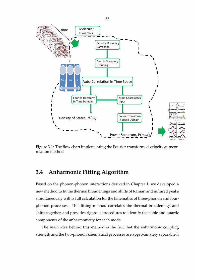
55
me
150 160 170 180 190
300K
500K
700K
900K
(a)
2GPa4GPa6GPa
520 540 560 580
Frequency (cm-1)
Frequency (cm-1) Frequency (cm
-1)
300K
500K
700K
900K(c)
365 385 405 425
(b)
300K
500K
700K
900K
g(k
,ω)
g(k
,ω)
Periodic Boundary
Correcon
Atomic Trajectory
Grouping
Auto-Correlaon In Time Space
Fourier Transform
In Time Domain
Atom Coordinates
Input
Fourier Transform
In Space DomainDensity of States,
Power Spectrum, P
Molecular
Dynamics
ALL
Figure 3.1: The flow chart implementing the Fourier-transformed velocity autocor-relation method
3.4 Anharmonic Fitting Algorithm
Based on the phonon-phonon interactions derived in Chapter 1, we developed a
new method to fit the thermal broadenings and shifts of Raman and infrared peaks
simultaneously with a full calculation for the kinematics of three-phonon and four-
phonon processes. This fitting method correlates the thermal broadenings and
shifts together, and provides rigorous procedures to identify the cubic and quartic
components of the anharmonicity for each mode.
The main idea behind this method is the fact that the anharmonic coupling
strength and the two-phonon kinematical processes are approximately separable if

56
the anharmonicity tensor does not vary significantly for different phonon processes.
An analytical form of anharmonicity tensor was proposed by Ipatova [46], and more
recently was found to be a good approximation by first principles calculations
[47, 48] .
V( j; q1 j1; ...; qs−1 js−1) =1
2s!
(~
2N
) s2
N∆(q1 + · · · + qs−1)
×[ω j0ω1 · · · ωs−1 ]12 C( j; q1 j1; ...; qs−1 js−1) (3.24)
where ∆(q1 + · · · + qs−1) enforces momentum conservation. We consider the term
C( j; q1 j1; ...; qs−1 js−1) to be a constant of the Raman mode j, and we use it as a fit-
ting parameter. This approximation is not rigorous because C( j; q1 j1; q2 j2) and
C( j; j; q1 j1;−q1 j1) change with j1 and j2, but an average over modes, ⟨C(.)⟩ =∑1,2 C( j; q1 j1; q2 j2)/
∑1,2 1, is found by the fitting, where 1, 2 under the summation
symbol represent qi ji.
Central to this method is the calculation of the two-phonon DOS, D(Ω), defined
as
D(Ω) =∑q1, j1
∑q2 j2
D(Ω,ω1,ω2)
=1N
∑q1, j1
∑q2, j2
∆(q1 + q2)[(n1 + n2 + 1) δ(Ω − ω1 − ω2)
+ 2(n1 − n2) δ(Ω+ ω1 − ω2)]
(3.25)
which counts the number of phonon-phonon interaction channels available to a
phonon of frequencyΩ. It depends on temperature through the phonon occupancy
factors, n, and satisfies the kinematical conditions of conservation of energy and
momentum. The first and second terms in square brackets in Eq. 6.5 are from
down-conversion and up-conversion processes, respectively [47]. This spectral
quantity can be calculated by scanning all phonon modes in Brillouin zone.
We will discuss this algorithm in detail, and present examples of analyzing the
anharmonicity strengths of rutile and cuprite structures in the next few chapters.

57
Chapter 4
Phonon Anharmonicity of Rutile TiO2
The main content of this chapter appeared in the journal article: Tian Lan, Xiaoli
Tang and Brent Fultz, Physical Review B 85, 094305 (2012).
58
Raman spectra of rutile titanium dioxide (TiO2) were measured at temperatures
from 100 K to 1150 K. Each Raman mode showed unique changes with temperature.
Beyond the volume-dependent quasiharmonicity, the explicit anharmonicity was
large. A new method was developed to fit the thermal broadenings and shifts of
Raman peaks with a full calculation of the kinematics of 3-phonon and 4-phonon
processes, allowing the cubic and quartic components of the anharmonicity to be
identified for each Raman mode. A dominant role of phonon-phonon kinematics
on phonon shifts and broadenings is reported. Force field molecular dynamics
(MD) calculations with the Fourier-transformed velocity autocorrelation method
were also used to perform a quantitative study of anharmonic effects, successfully
accounting for the anomalous phonon anharmonicity of the B1g mode.
4.1 Introduction
Rutile is the most common and stable crystal structure of titanium dioxide (TiO2),
and is important for both science and technology. Owing to its high refractive
index and strong ultraviolet resistance, it is used extensively for pigments, optical
coatings and sunscreens. In the past two decades, TiO2 surfaces have been subjects
of research as photocatalysts and high efficiency solar cells [49–53]. Many questions
remain about point defects, vibrational dynamics, size effects and the recently-
reported close relationship between surface and bulk properties [53–55]. A better
understanding of the lattice dynamics of rutile will help answer many of them.
Rutile TiO2 is tetragonal with the space group P4/mnm. It is stable to 1800 K
[56]. The other two naturally-occurring phases of TiO2, anatase and brookite, are
metastable and both convert to rutile upon heating. The 15 optical vibrational
modes of rutile TiO2 have the irreducible representation 1A1g+ 1A2g+ 1A2u+ 1B1g+
1B2g + 2B1u + 1Eg + 3Eu. The modes of symmetry B1g, Eg, A1g and B2g are Raman
active. The Raman active modes comprise motions of anions with respect to sta-
tionary central cations, either perpendicular to the c axis (modes B1g, A1g and B2g),
or along the c axis (mode Eg). The Raman spectrum of rutile was first recorded

59
by Narayanan [57], and peak assignments were made by Porto, et al. [58]. Ra-
man spectrometry has been used in many studies of the lattice dynamics, phase
transition and nanostructures of TiO2 [59–64].
The present work on rutile TiO2 focuses on anharmonicity, one of the most
important but poorly understood characteristics of lattice dynamics at elevated
temperatures. Anharmonic behavior affects crystal stability, heat capacity, optical
properties and thermal transport. It causes shifts of phonon energies with tempera-
ture because larger thermal displacements emphasize components of the potential
with higher powers of the displacement. Phonon broadening from decreased life-
times is another anharmonic phenomenon, and an anharmonic model should be
able to predict both the broadenings and shifts of the phonons with temperature. To
date there have been few studies of anharmonicity of rutile TiO2. Perhaps the most
complete experimental results are from Samara and Peercy’s work in 1973 [59].
They reported frequency shifts of Raman modes with temperature and pressure,
although the temperature range was below 500 K and no broadening information
was reported. Their results show that the B1g mode, which comprises rotatory mo-
tions of the four nearest neighbor oxygen anions around a central titanium atom
(Fig. 4.1) is especially interesting. Its frequency changes little with temperature,
but softens with pressure. Studies on other materials with the rutile structure, e.g.,
SnO2, MgF2 and FeF2 report similar behavior of the B1g mode [65–68]. There are
two conflicting views on the physical origin of these anomalies. One attributes it
to an incipient structural phase transition [65, 69, 70], and the other attributes it to
a thermal- or pressure-induced lattice contraction [66–68].
Lattice dynamics calculations based on density functional theory (DFT) were
used to study the effect of pressure on phonons in rutile TiO2 [70, 71]. These
calculations were for low temperature and in the quasiharmonic approximation,
where phonons are assumed to be harmonic but their frequencies change with
volume. Only a few studies have used molecular dynamics (MD) to calculate
anharmonic frequency shifts and broadenings of phonon mode of materials [72,73],
and to our knowledge, no such investigation has yet been performed on rutile TiO2.
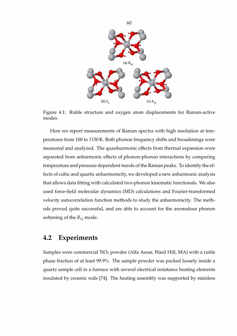
60
(a) B1g
(c) A1g(b) Eg
Figure 4.1: Rutile structure and oxygen atom displacements for Raman-activemodes.
Here we report measurements of Raman spectra with high resolution at tem-
peratures from 100 to 1150 K. Both phonon frequency shifts and broadenings were
measured and analyzed. The quasiharmonic effects from thermal expansion were
separated from anharmonic effects of phonon-phonon interactions by comparing
temperature and pressure dependent trends of the Raman peaks. To identify the ef-
fects of cubic and quartic anharmonicity, we developed a new anharmonic analysis
that allows data fitting with calculated two-phonon kinematic functionals. We also
used force-field molecular dynamics (MD) calculations and Fourier-transformed
velocity autocorrelation function methods to study the anharmonicity. The meth-
ods proved quite successful, and are able to account for the anomalous phonon
softening of the B1g mode.
4.2 Experiments
Samples were commercial TiO2 powder (Alfa Aesar, Ward Hill, MA) with a rutile
phase fraction of at least 99.9%. The sample powder was packed loosely inside a
quartz sample cell in a furnace with several electrical resistance heating elements
insulated by ceramic rods [74]. The heating assembly was supported by stainless

61
steel flanges and surrounded by heat shields made of niobium foil. The assembly
was mounted in a quartz optical tube of 1 mm thickness, and evacuated with a
turbomolecular pump. Both the interior and exterior of the tube were covered by
aluminum foil for thermal radiation shielding. A temperature controller drove a
1 kW direct current power supply for heating power. For low temperature measure-
ments, the sample cell was mounted on the copper cold finger of a liquid nitrogen
filled cryostat and evacuated. Uniformity of sample temperature was confirmed by
multiple ultrafine thermocouples mounted at different locations inside the sample
cell, and the temperature resolution was ±1 K. Samples were measured at tem-
peratures from 100 to 1150 K, with intervals of 100 K below 700 K and 50 K above
700 K.
The Raman spectrometer used the 532 nm line from a solid state laser at power
levels of 100 mW or less. A high efficiency longpass edge filter was used to block
the laser line. The single pass spectrometer (Princeton Instruments Acton Series
500 mm) used a two-dimensional charge-coupled device camera with thermoelec-
tric cooling (Princeton Instruments PIXIS 400B). The instrument resolution was
1.4 cm−1. Each Raman spectrum was accumulated in 10 measurements with 1 s
exposure times.
4.3 Molecular Dynamics Calculations
Our classical molecular dynamics (MD) calculations used simulation tools in the
GULP software package [75]. Rutile TiO2, with its relatively small ionicity and large
dipole moments on anions, is a challenging system for developing an interatomic
potential. Few of those we tried [76–79] could simultaneously provide the crystal
structure, elastic properties, thermal expansion and phonon vibrational frequen-
cies. The best results for phonon properties were obtained with the Buckingham
potential (Model 3) developed by Mostoller and Wang (MW shell model) [79]. The
MW shell model was parameterized by fitting the phonon spectra over the whole
Brillouin zone, and the model also gives reasonable bulk properties. We altered
62
slightly this model to improve its transferability and stability at different temper-
atures and pressures (the shell charge of titanium atoms was increased to 0.37 |e|).The parameters of the force field model were fixed for all the calculations presented
below.
To extract anharmonic information on individual phonon modes from the
atomic trajectories of the MD simulations, the phonon spectral energy density
function g(q,ω) was obtained by the velocity autocorrelation technique [43, 80]
g(q,ω) =∫
dt e−iωt∑n,b
ei q·Rn ⟨vn,b(t) v0,0(0)⟩ (4.1)
where ⟨ ⟩ is an ensemble average, vn,b(t) is the velocity of the atom b in the unit
cell n at time t, Rn is the equilibrium position of the cell n, and q is the phonon
wavevector. Equation 4.1 is both a time and space Fourier transform, and gives the
frequency and lifetime of each phonon mode with a resolution determined by the
size of the supercell used in the simulation.
Our MD simulations were performed with a 2×2×20 supercell containing 960
atom cores and shells. We used the Verlet algorithm, an NPT ensemble, and a
modified Nose-Hoover thermostat for control of temperature and pressure. Both
the isobaric temperature-dependent phonon peaks and the isothermal pressure-
dependent phonon peaks were obtained in ranges of 300 K to 900 K and 0 GPa to
6 GPa. The run time for each set was 100 ps with time steps of 0.5 fs and sampling
periods of 10 fs. The time-dependent atomic trajectories of velocity were post-
processed by the velocity autocorrelation method to obtain mode frequencies and
linewidths. The resolution of the wavevector q along theΓ-Z direction was therefore
Gz/20, where Gz is the magnitude of the reciprocal lattice vector. The frequency
resolution was approximately 0.5 cm−1.
63
4.4 Results
4.4.1 Experiment
After background subtraction, each peak in each spectrum was fitted to a Lorentzian
function to obtain a centroid and full-width-at-half-maximum (FWHM). The FWHM
data from the experiment were corrected for the finite resolution of the spectrome-
ter [81]. Figure 4.3 presents these results of peak shifts and widths versus temper-
ature. At room temperature, the Raman peak frequencies were 143 cm−1, 447 cm−1
and 612 cm−1, consistent with the well-accepted data from Porto, et al. [58]. We
also find good agreement with the frequency shift data reported by Samara and
Peercy [59] at temperatures below 480 K.
The Eg mode undergoes a large phonon softening with temperature. The A1g
mode has a small thermal softening at high temperature, but below 400 K the A1g
mode tends to stiffen slightly with temperature, as also reported by Samara and
Peercy [59]. The B1g mode appears to have no thermal shift. The thermal broaden-
ings of Eg and A1g peaks are large, but the B1g mode shows far less broadening.
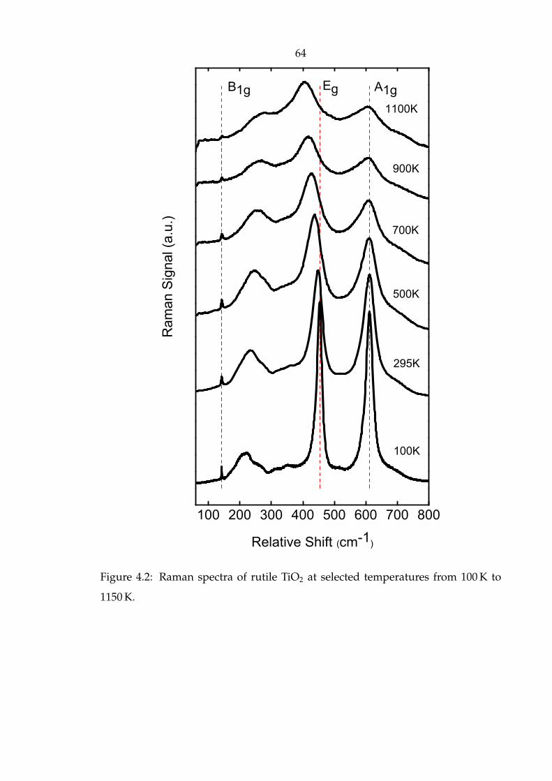
64
100 200 300 400 500 600 700 800
A1gEg
1100K
900K
700K
500K
295K
Ram
an S
ignal (a
.u.)
Relative Shift (cm-1)
100K
B1g
Figure 4.2: Raman spectra of rutile TiO2 at selected temperatures from 100 K to
1150 K.
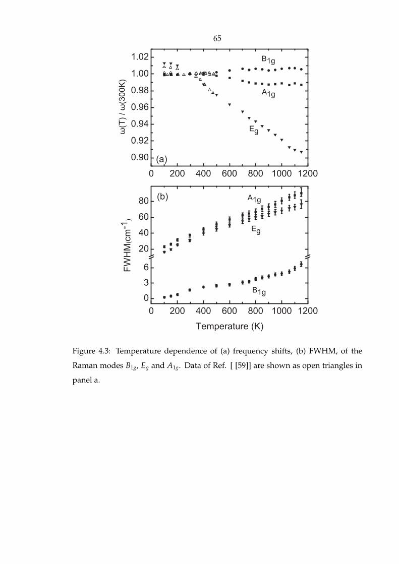
65
0 200 400 600 800 1000 1200
0.90
0.92
0.94
0.96
0.98
1.00
1.02
(a)
B1g
A1g
Eg
Eg
A1g
B1g
(b)
0 200 400 600 800 1000 1200
0
3
6
20
40
60
80
FW
HM
(cm
-1)
Temperature (K)
ω(T
) / ω
(300K
)
Figure 4.3: Temperature dependence of (a) frequency shifts, (b) FWHM, of the
Raman modes B1g, Eg and A1g. Data of Ref. [ [59]] are shown as open triangles in
panel a.
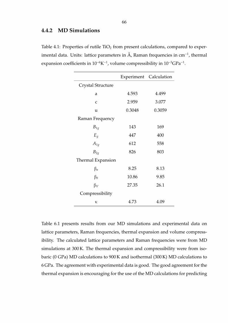
66
4.4.2 MD Simulations
Table 4.1: Properties of rutile TiO2 from present calculations, compared to exper-
imental data. Units: lattice parameters in Å, Raman frequencies in cm−1, thermal
expansion coefficients in 10−6K−1, volume compressibility in 10−3GPa−1.
Experiment Calculation
Crystal Structure
a 4.593 4.499
c 2.959 3.077
u 0.3048 0.3059
Raman Frequency
B1g 143 169
Eg 447 400
A1g 612 558
B2g 826 803
Thermal Expansion
βa 8.25 8.13
βb 10.86 9.85
βV 27.35 26.1
Compressibility
κ 4.73 4.09
Table 6.1 presents results from our MD simulations and experimental data on
lattice parameters, Raman frequencies, thermal expansion and volume compress-
ibility. The calculated lattice parameters and Raman frequencies were from MD
simulations at 300 K. The thermal expansion and compressibility were from iso-
baric (0 GPa) MD calculations to 900 K and isothermal (300 K) MD calculations to
6 GPa. The agreement with experimental data is good. The good agreement for the
thermal expansion is encouraging for the use of the MD calculations for predicting

67
anharmonic behavior.
Figure 4.4a presents simulated Raman peaks of the B1g mode at elevated tem-
peratures at 0 GPa, and at elevated pressures at 300 K. The small thermal shift
and broadening seen in the experimental results of Fig. 5.2 are apparent in the
simulated results.
Figure 4.4b, c presents simulated Raman peaks of the Eg and A1g modes at
elevated temperature. The large thermal broadening of both modes, and the large
thermal shift of the Eg mode are in apparent agreement with the experimental
results of Fig. 5.2.
4.5 Experimental Data Analysis
4.5.1 Analysis of Quasiharmonicity and Anharmonicity
Both quasiharmonicity and explicit anharmonicity contribute to the non-harmonic
lattice dynamics of rutile TiO2. In the quasiharmonic model, phonon modes be-
have harmonically with infinite lifetimes, but their frequencies are changed by the
effects of volume on the interatomic potential. Explicit anharmonicity originates
with phonon-phonon interactions, which increase with temperature. Explicit an-
harmonicity contributes to shifts in phonon frequencies, but also causes phonon
damping and lifetime broadening of phonon peaks with temperature. The large
peak broadenings and peculiar differences in shifts of the Raman peaks in rutile
TiO2 suggest there are important effects from explicit anharmonicity.
To separate the effects of quasiharmonicity and explicit anharmonicity, we treat
the mode frequency ω j = ω j(V,T) as a function of volume and temperature [59]
(∂ lnω j
∂T
)P= −β
κ
(∂ lnω j
∂P
)T+
(∂ lnω j
∂T
)V
(4.2)
where j is the phonon mode index, β is the volume thermal expansivity and κ is the
isothermal compressibility. The left-hand side gives the temperature-dependent

68
150 160 170 180 190
300K
500K
700K
900K
(a)
2GPa4GPa6GPa
520 540 560 580
Frequency (cm-1)
Frequency (cm-1) Frequency (cm
-1)
300K
500K
700K
900K(c)
365 385 405 425
(b)
300K
500K
700K
900K
g(q
=0
,ω
)
g(q
=0
,ω
)
Figure 4.4: (a) The B1g Raman peak calculated from the velocity trajectories ofMD simulations, at temperatures as labeled and constant pressure of 0 GPa, and atpressures from 0 to 6 GPa at 300 K. (b) Calculated Eg Raman peak, and (c) CalculatedA1g Raman peak at temperatures as labeled and constant pressure of 0 GPa. Solidred curves are the Lorentzian fits.

69
isobaric frequency shift, including both quasiharmonic and explicit anharmonic
behavior. The first term on the right-hand side, the isothermal frequency shift as a
function of pressure, is the quasiharmonic contribution to the frequency shift. By
defining a mode Gruneisen parameter as the proportionality of the relative change
of the mode frequency to the relative change of volume, i.e., γ j = −∂(lnω j)/(∂(ln V)),
this term can be written as γ jβ. The second term on the right of Eq. 6.7 is the pure
temperature contribution to the frequency shift from the explicit anharmonicity.
From the difference of the isobaric and isothermal frequency shifts, the explicit
anharmonicity can be determined experimentally.
We used the mode Gruneisen parameters γ j reported by Samara and Peercy [59]
from Raman measurements under pressure. Since the γ j are very weakly depen-
dent on temperature [59,65], as is the thermal expansion above 300 K [82], the γ j can
be assumed to be constants for identifying the volume dependent quasiharmonic
contribution. The results, summarized in Table 5.2, separate the frequency shifts
from quasiharmonicity and explicit anharmonicity. Samara and Peercy’s results at
296 K are also shown for comparison. For the B1g mode, Table 5.2 shows that the
quasiharmonic and explicit anharmonic contributions are both large but opposite
in sign, and their near-perfect cancellation causes the B1g mode to have a small
thermal frequency shift to 1150 K. The quasiharmonic softening of the B1g mode
with increasing pressure (or equivalently, with decreasing temperature), and its
negative Gruneisen parameter, are anomalous. The A1g mode has a similar can-
cellation of quasiharmonic and explicit anharmonic contributions, but the signs of
two contributions are reversed. The positive explicit anharmonic shift of the A1g
mode is unusual. We find this explicit anharmonicity at higher temperature to be
smaller than Samara and Peercy’s result below 400 K. There is a similar difference
for the Eg mode but with an opposite trend, where the explicit anharmonic contri-
bution increases by an order of magnitude when averaged over a larger range of
temperature. It becomes comparable to the quasiharmonic contribution, hastening
the softening of the Eg mode at temperatures above 400 K.
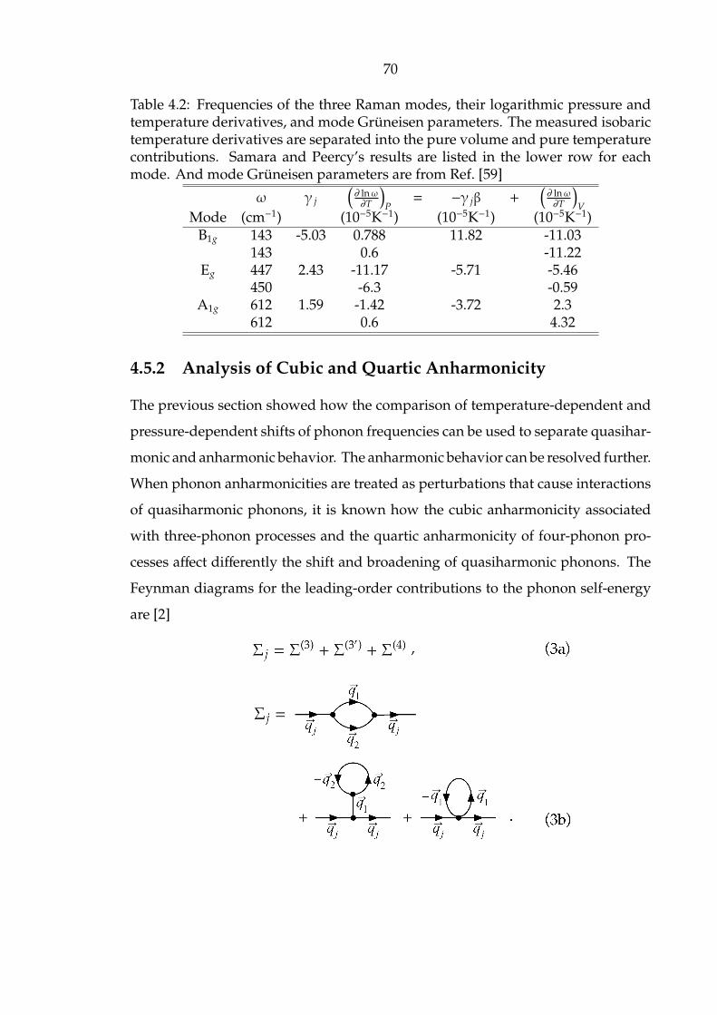
70
Table 4.2: Frequencies of the three Raman modes, their logarithmic pressure andtemperature derivatives, and mode Gruneisen parameters. The measured isobarictemperature derivatives are separated into the pure volume and pure temperaturecontributions. Samara and Peercy’s results are listed in the lower row for eachmode. And mode Gruneisen parameters are from Ref. [59]
ω γ j
(∂ lnω∂T
)P= −γ jβ +
(∂ lnω∂T
)V
Mode (cm−1) (10−5K−1) (10−5K−1) (10−5K−1)B1g 143 -5.03 0.788 11.82 -11.03
143 0.6 -11.22Eg 447 2.43 -11.17 -5.71 -5.46
450 -6.3 -0.59A1g 612 1.59 -1.42 -3.72 2.3
612 0.6 4.32
4.5.2 Analysis of Cubic and Quartic Anharmonicity
The previous section showed how the comparison of temperature-dependent and
pressure-dependent shifts of phonon frequencies can be used to separate quasihar-
monic and anharmonic behavior. The anharmonic behavior can be resolved further.
When phonon anharmonicities are treated as perturbations that cause interactions
of quasiharmonic phonons, it is known how the cubic anharmonicity associated
with three-phonon processes and the quartic anharmonicity of four-phonon pro-
cesses affect differently the shift and broadening of quasiharmonic phonons. The
Feynman diagrams for the leading-order contributions to the phonon self-energy
are [2]
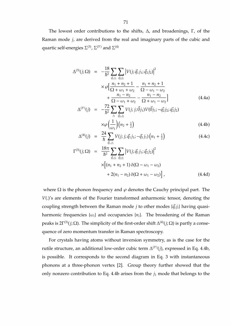
71
The lowest order contributions to the shifts, ∆, and broadenings, Γ, of the
Raman mode j, are derived from the real and imaginary parts of the cubic and
quartic self-energies Σ(3), Σ(3′) and Σ(4)
∆(3)( j;Ω) = −18~2
∑q1 j1
∑q2 j2
∣∣∣V( j; q1 j1; q2 j2)∣∣∣2
×℘[ n1 + n2 + 1Ω+ ω1 + ω2
− n1 + n2 + 1Ω − ω1 − ω2
+n1 − n2
Ω − ω1 + ω2− n1 − n2
Ω+ ω1 − ω2
](4.4a)
∆(3′)( j) = −72~2
∑j1
∑q2, j2
V( j; j; 0 j1)V(0 j1;−q2 j2; q2 j2)
×℘( 1ω1
) (n2 +
12
)(4.4b)
∆(4)( j) =24~
∑q1, j1
V( j; j; q1 j1;−q1 j1)(n1 +
12
)(4.4c)
Γ(3)( j;Ω) =18π~2
∑q1 j1
∑q2 j2
∣∣∣V( j; q1 j1; q2 j2)∣∣∣2
×[(n1 + n2 + 1) δ(Ω − ω1 − ω2)
+ 2(n1 − n2) δ(Ω+ ω1 − ω2)], (4.4d)
where Ω is the phonon frequency and ℘ denotes the Cauchy principal part. The
V(.)’s are elements of the Fourier transformed anharmonic tensor, denoting the
coupling strength between the Raman mode j to other modes qi ji having quasi-
harmonic frequencies ωi and occupancies ni. The broadening of the Raman
peaks is 2Γ(3)( j;Ω). The simplicity of the first-order shift ∆(4)( j;Ω) is partly a conse-
quence of zero momentum transfer in Raman spectroscopy.
For crystals having atoms without inversion symmetry, as is the case for the
rutile structure, an additional low-order cubic term ∆(3′)( j), expressed in Eq. 4.4b,
is possible. It corresponds to the second diagram in Eq. 3 with instantaneous
phonons at a three-phonon vertex [2]. Group theory further showed that the
only nonzero contribution to Eq. 4.4b arises from the j1 mode that belongs to the

72
identity representation [83]. Owing to the rigorous restrictions on the existence
of instantaneous three-phonon processes, ∆(3′) is generally much smaller than ∆(3).
For rutile TiO2, this term needs to be evaluated only for the A1g mode because it
does not have inversion symmetry for oxygen atom motions (see Fig. 4.1c).
Including all shifts, the frequencies of the Raman peaks are
ω j(T,Ω) = ω j0 exp[−γ j
∫ T
0β(T) dT
]+ ∆(3)( j;Ω)
+∆(3′)( j) + ∆(4)( j) . (4.5)
The first term on the right of Eq. 4.5 is the integral form of the quasiharmonic phonon
shift (discussed after Eq. 6.7) and from the last term of Eq. 4.5, (∂ω j/∂T)V δT =
∆(3)( j;Ω) + ∆(3′)( j) + ∆(4)( j) is the explicit anharmonic shift. To obtain β(T), experi-
mental data from 4 K to 1200 K [59, 82] were fitted with a well-accepted analytical
form [84]
β(T) =(A
T+
BT2
)sinh−2
(T1
T
)(4.6)
giving A = 7.16 × 10⁻⁵, B = 0.524K and T1 = 146.2K.
In what follows, we use Eqns. 4.4a - 4.4d, to identify the magnitudes and signs
of the cubic and quartic anharmonicities from the thermal shifts and broadenings
of the Raman modes in rutile TiO2. We do not calculate the V(.)’s, which are
complicated tensor quantities, but instead we treat them as parameters in fitting
the experimental trends of the Raman modes. We do a full calculation of the
two-phonon density of states, however, as described below.
From Ipatova, et al. [46], an anharmonic tensor element for a process with s
phonons is
V( j; q1 j1; ...; qs−1 js−1) =1
2s!
(~
2N
) s2
N∆(q1 + · · · + qs−1)
×[ω j0ω1 · · · ωs−1 ]12 C( j; q1 j1; ...; qs−1 js−1) (4.7)
where ∆(q1 + · · · + qs−1) enforces momentum conservation. Ipatova, et al. [46],

73
suggest that the C(.)’s are slowly-varying functions of their arguments. Several
studies used this assumption to calculate or fit approximately the anharmonic
broadening [46, 85, 86]. Klemens assumed the frequency independent part of the
coupling tensor for a Raman mode j was a constant that depended on the strain field
of the mode [87]. Likewise, we consider the term C( j; q1 j1; ...; qs−1 js−1) to be a constant
of the Raman mode j, and we use it as a fitting parameter. This approximation is
not rigorous because C( j; q1 j1; q2 j2) and C( j; j; q1 j1;−q1 j1) change with j1 and j2, but
an average over modes, ⟨C(.)⟩ = ∑1,2 C( j; q1 j1; q2 j2)/
∑1,2 1, is found by the fitting,
where 1, 2 under the summation symbol represent qi ji. We define the cubic and
quartic fitting parameters as
C(3)j = ⟨C( j; q1 j1; q2 j2)⟩ (4.8a)
C(4)j = ⟨C( j; j; q1 j1;−q1 j1)⟩ (4.8b)
While the anharmonic tensor describes the coupling strength of phonon-phonon
interactions, a prerequisite is that the phonons in these processes satisfy the kine-
matical conditions of conservation of energy and momentum (as explicitly written
in Eqs. 4.4 and 6.2). Central to phonon linewidth broadening from the cubic anhar-
monicity, 2Γ(3), is the two-phonon DOS, D(Ω), defined as
D(Ω) =∑q1, j1
∑q2 j2
D(Ω,ω1,ω2)
=1N
∑q1, j1
∑q2, j2
∆(q1 + q2)[(n1 + n2 + 1) δ(Ω − ω1 − ω2)
+ 2(n1 − n2) δ(Ω+ ω1 − ω2)]
(4.9)
which depends on temperature through the phonon occupancy factors, n. The first
and second terms in square brackets in Eq. 6.5 are from down-conversion and up-
conversion processes, respectively [47]. The two-phonon kinematical functional
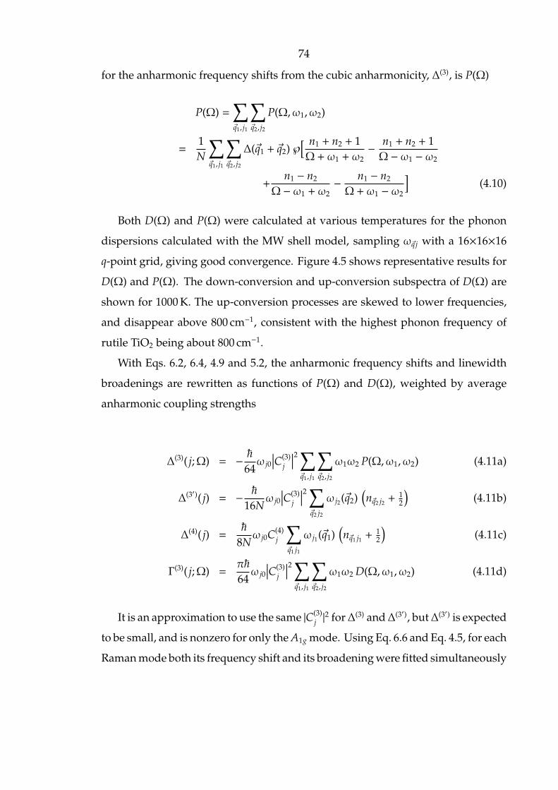
74
for the anharmonic frequency shifts from the cubic anharmonicity, ∆(3), is P(Ω)
P(Ω) =∑q1, j1
∑q2, j2
P(Ω,ω1,ω2)
=1N
∑q1, j1
∑q2, j2
∆(q1 + q2) ℘[ n1 + n2 + 1Ω+ ω1 + ω2
− n1 + n2 + 1Ω − ω1 − ω2
+n1 − n2
Ω − ω1 + ω2− n1 − n2
Ω+ ω1 − ω2
](4.10)
Both D(Ω) and P(Ω) were calculated at various temperatures for the phonon
dispersions calculated with the MW shell model, sampling ωq j with a 16×16×16
q-point grid, giving good convergence. Figure 4.5 shows representative results for
D(Ω) and P(Ω). The down-conversion and up-conversion subspectra of D(Ω) are
shown for 1000 K. The up-conversion processes are skewed to lower frequencies,
and disappear above 800 cm−1, consistent with the highest phonon frequency of
rutile TiO2 being about 800 cm−1.
With Eqs. 6.2, 6.4, 4.9 and 5.2, the anharmonic frequency shifts and linewidth
broadenings are rewritten as functions of P(Ω) and D(Ω), weighted by average
anharmonic coupling strengths
∆(3)( j;Ω) = − ~64ω j0
∣∣∣C(3)j
∣∣∣2 ∑q1, j1
∑q2, j2
ω1ω2 P(Ω,ω1,ω2) (4.11a)
∆(3′)( j) = − ~16Nω j0
∣∣∣C(3)j
∣∣∣2 ∑q2 j2
ω j2(q2)(nq2 j2 +
12
)(4.11b)
∆(4)( j) =~
8Nω j0C(4)
j
∑q1 j1
ω j1(q1)(nq1 j1 +
12
)(4.11c)
Γ(3)( j;Ω) =π~64ω j0
∣∣∣C(3)j
∣∣∣2 ∑q1, j1
∑q2, j2
ω1ω2 D(Ω,ω1,ω2) (4.11d)
It is an approximation to use the same |C(3)j |2 for∆(3) and∆(3′), but∆(3′) is expected
to be small, and is nonzero for only the A1g mode. Using Eq. 6.6 and Eq. 4.5, for each
Raman mode both its frequency shift and its broadening were fitted simultaneously

75
with the two parameters, |C(3)j |2 and C(4)
j . The best fits for the shifts and broadenings
are shown in Figs. 4.6, 4.7 and 4.8, and the fitting parameters are given in Table
5.3. Figure 4.6a, 4.7a and 4.8a also present contributions to the shift from the
quasiharmonic and explicit anharmonicity as dashed curves.
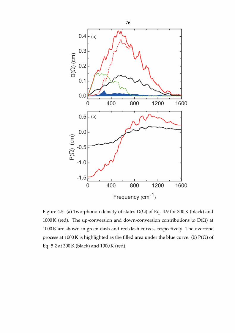
76
0 400 800 1200 1600
0.0
0.1
0.2
0.3
0.4 (a)
D(Ω
) (c
m)
(b)
0 400 800 1200 1600
-1.5
-1.0
-0.5
0.0
0.5
P(Ω
) (
cm
)
Frequency (cm-1)
Figure 4.5: (a) Two-phonon density of states D(Ω) of Eq. 4.9 for 300 K (black) and
1000 K (red). The up-conversion and down-conversion contributions to D(Ω) at
1000 K are shown in green dash and red dash curves, respectively. The overtone
process at 1000 K is highlighted as the filled area under the blue curve. (b) P(Ω) of
Eq. 5.2 at 300 K (black) and 1000 K (red).
77
Temperature (K)
0 200 400 600 800 1000 1200130
135
140
145
150
155
160
165
Ra
ma
n S
hift
(cm
-1)
(a)
0 200 400 600 800 1000 12000
1
2
3
4
5
6
7
FW
HM
(cm
-1)
(b)
Figure 4.6: Temperature dependence of parameters for fittings to Raman peaks of
mode B1g (a) frequency shift, and (b) FWHM. Solid circles are experimental data.
Solid curves are the fittings of the experimental points to Eq. 4.5 and Eq. 4.11d.
Dotted line is the quasiharmonic contribution to the frequency shift. Dash-dot line
is the explicit anharmonicity ω0 + ∆(4) + ∆(3), and dashed line is ω0 + ∆
(3).

78
Temperature (K)
0 200 400 600 800 1000 1200390
400
410
420
430
440
450
460
Ra
ma
n S
hift
(cm
-1)
(a)
0 200 400 600 800 1000 120010
20
30
40
50
60
70
80
FW
HM
(cm
-1)
(b)
Figure 4.7: Temperature dependence of parameters for fittings to Raman peaks
of mode Eg (a) frequency shift, and (b) FWHM. Dotted line is the quasiharmonic
contribution to the frequency shifts. Dash-dot line is the explicit anharmonicity
ω0 + ∆(4) + ∆(3) and dashed line is ω0 + ∆
(3).
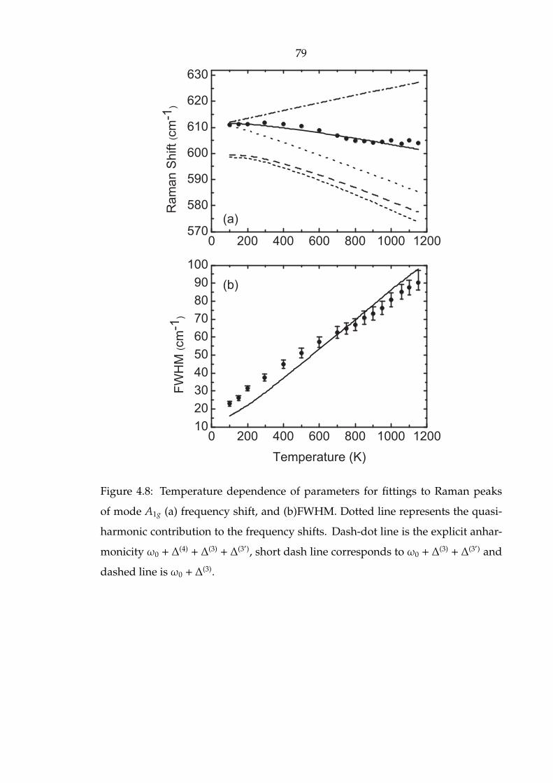
79
0 200 400 600 800 1000 120010
20
30
40
50
60
70
80
90
100
FW
HM
(cm
-1)
Temperature (K)
(b)
0 200 400 600 800 1000 1200570
580
590
600
610
620
630
Ra
ma
n S
hift
(cm
-1)
(a)
Figure 4.8: Temperature dependence of parameters for fittings to Raman peaks
of mode A1g (a) frequency shift, and (b)FWHM. Dotted line represents the quasi-
harmonic contribution to the frequency shifts. Dash-dot line is the explicit anhar-
monicity ω0 + ∆(4) + ∆(3) + ∆(3′), short dash line corresponds to ω0 + ∆
(3) + ∆(3′) and
dashed line is ω0 + ∆(3).
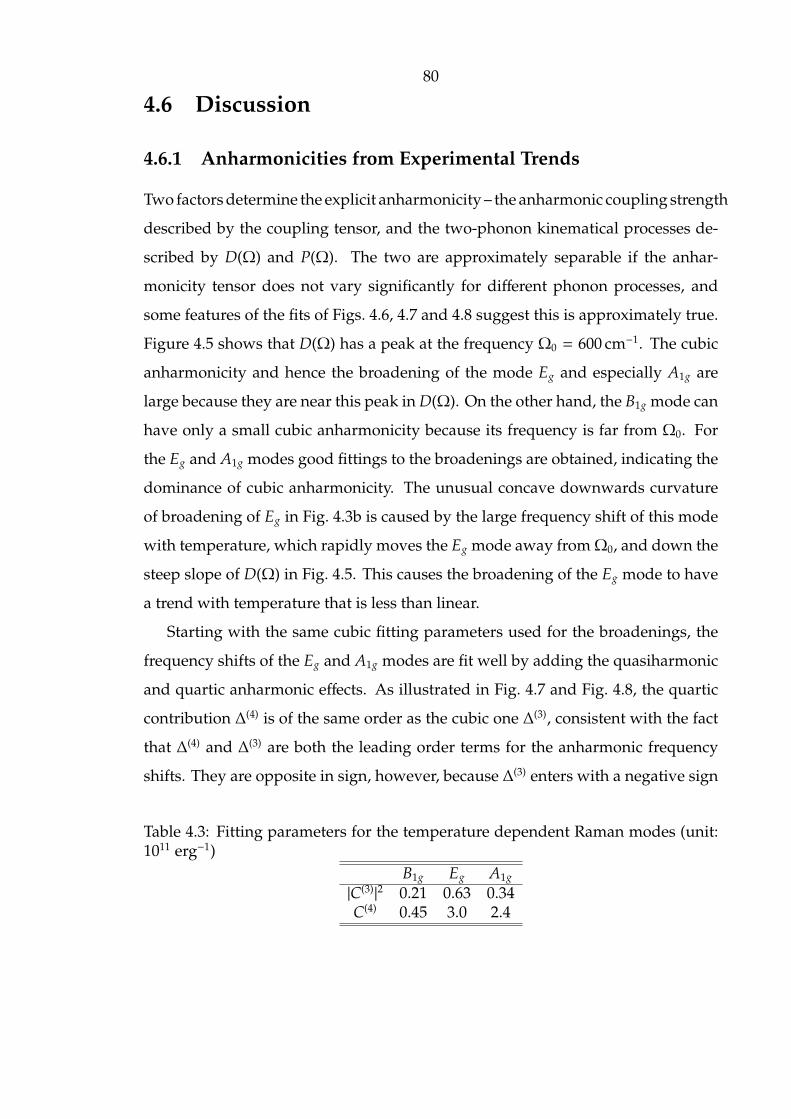
80
4.6 Discussion
4.6.1 Anharmonicities from Experimental Trends
Two factors determine the explicit anharmonicity – the anharmonic coupling strength
described by the coupling tensor, and the two-phonon kinematical processes de-
scribed by D(Ω) and P(Ω). The two are approximately separable if the anhar-
monicity tensor does not vary significantly for different phonon processes, and
some features of the fits of Figs. 4.6, 4.7 and 4.8 suggest this is approximately true.
Figure 4.5 shows that D(Ω) has a peak at the frequency Ω0 = 600 cm−1. The cubic
anharmonicity and hence the broadening of the mode Eg and especially A1g are
large because they are near this peak in D(Ω). On the other hand, the B1g mode can
have only a small cubic anharmonicity because its frequency is far from Ω0. For
the Eg and A1g modes good fittings to the broadenings are obtained, indicating the
dominance of cubic anharmonicity. The unusual concave downwards curvature
of broadening of Eg in Fig. 4.3b is caused by the large frequency shift of this mode
with temperature, which rapidly moves the Eg mode away fromΩ0, and down the
steep slope of D(Ω) in Fig. 4.5. This causes the broadening of the Eg mode to have
a trend with temperature that is less than linear.
Starting with the same cubic fitting parameters used for the broadenings, the
frequency shifts of the Eg and A1g modes are fit well by adding the quasiharmonic
and quartic anharmonic effects. As illustrated in Fig. 4.7 and Fig. 4.8, the quartic
contribution ∆(4) is of the same order as the cubic one ∆(3), consistent with the fact
that ∆(4) and ∆(3) are both the leading order terms for the anharmonic frequency
shifts. They are opposite in sign, however, because ∆(3) enters with a negative sign
Table 4.3: Fitting parameters for the temperature dependent Raman modes (unit:1011 erg−1)
B1g Eg A1g
|C(3)|2 0.21 0.63 0.34C(4) 0.45 3.0 2.4
81
times the square of the cubic coupling tensor. The net anharmonic shift is usually
negative, as for the Eg mode. For the A1g mode, the additional contribution from
the instantaneous three-phonon processes, ∆(3′) is also considered, but owing to a
symmetry restriction, this term is small. The A1g mode is unusual, having a net
anharmonic shift that is positive, indicating the quartic contribution to the shift is
larger than the cubic. Figure 4.5 shows that, at the frequency of mode A1g, P(Ω)
is close to zero. The cubic anharmonic shift ∆(3) is therefore attenuated for the A1g
mode.
For the B1g mode, Fig. 4.6a shows that the fitting deviates substantially from the
experimental data. The discrepancies may originate with anharmonic contribu-
tions beyond the leading terms we considered. The rapid increase of the linewidth
of the B1g mode above the Debye temperature (≃780 K for rutile TiO2) further sup-
ports this argument (a T2 dependence is typical of broadening from higher-order
quartic anharmonicity [46]).
The ratio of cubic to quartic anharmonicity is sometimes evaluated by fitting
Raman spectra to a simplified Klemens model, in which the shifts and broadenings
from phonon-phonon interactions (Eq. 4.4) include only overtone processes (one
optical phonon at the Γ point decays into two or three phonons of equal energy on
the same branch) [88]. In this simplified model, the temperature dependence of the
Raman peak linewidth is
Γ j(T) = Γ j(0) + A(1 +
2e~ω j0/2kBT − 1
)+ B
(1 +
3e~ω j0/3kBT − 1
+3
(e~ω j0/3kBT − 1)2
) (4.12)
where Γ j(0) is the FWHM extrapolated to 0 K, and A and B are fitting parameters
for three-phonon and four-phonon processes, respectively. A similar expression
is used to fit the frequency shift, with fitting parameters C, D replacing A, B, and
the quasiharmonic frequency shift replacing Γ j(0) in Eq. 4.12. This approach often
gives good fits to experimental Raman data, but the results can be misleading
owing to the oversimplified approximations. In performing such fits for our data

82
on rutile TiO2, we found a cubic anharmonicity for the B1g mode that was large
compared to the quartic, which we know to be incorrect. This approach also gave
a negative fitting parameter B for the quartic anharmonicity to explain the concave
curvature of the thermal broadening of the Eg mode, which is unreasonable. The
independent fits to thermal trends of linewidth and frequency shift (using Eq. 4.12
and its equivalent) offer no correlation between these quantities, even though they
share a dependence on the same cubic anharmonic coupling tensor. Furthermore,
it has been shown that the contributions from overtone processes are usually very
small [81], as is shown by the lowest curve in Fig. 4.5(a) for rutile TiO2.
4.6.2 Anharmonicities from MD Simulations
Figure 4.9 shows the effects of temperature on the frequency shifts and broadenings
of the B1g mode, obtained from MD results such as those of Fig. 4.4a. Also shown
is the effect of pressure on the frequency shift of the B1g mode. These results are in
excellent agreement with the experimental data.
From Fig. 4.9c, the Gruneisen parameter of the B1g mode is found to be −4.23,
which compares well to the experimental value of −5.03 reported by Samara and
Peercy [59].
To further study the anomalous anharmoncity of the B1g mode, the frozen
phonon method was used with the force field of MW shell model, allowing us to
obtain the effective potential energy curve of the B1g mode at different temperatures
and pressures, as shown in Fig. 4.10. Three sets of lattice parameters were used,
obtained from MD calculations at 300 K and 0 GPa, 300K and 6 GPa, 800 K and 0
GPa. These correspond to the volume at ambient conditions, a volume contraction
of about 2.4%, and a volume expansion by about 1.3%, respectively. The quadratic
potential dominates, and there is no cubic anharmonic contribution, as expected
from symmetry. The quartic anharmonic potential is significant, however.
Figure 4.10 shows that the harmonic part of the B1g potential has a curvature that
increases with volume, contrary to the usual trend. This anomalous quasiharmonic

83
response to volume reduces the force constant with increasing pressure, giving an
anomalous mode softening. This phenomenon can be explained by the transverse
motion of oxygen anion in the B1g mode, perpendicular to the Ti-O bond. This
transverse motion makes the mean interatomic distance ⟨R⟩ = |⟨rO − rTi⟩| greater
than the distance between the mean atomic positions R0 = |⟨rO⟩ − ⟨rTi⟩|. An in-
crease in volume increases the tension in the bond, tending to bring ⟨R⟩ closer
to R0. The restoring force for transverse motion is thus increased, and the mode
is stiffened [89]. For most materials this tension effect is hardly seen because the
stretching along the bond direction is usually dominant, and bond stretching weak-
ens the force constant. Rutile TiO2 is special owing to its open structure, which
reduces the coordination of atoms around the oxygen, allowing it large transverse
amplitudes. Moreover, the Ti-O bonds are strong (vibrational modes along this
bond direction, such as mode B2g, are at the highest frequencies). The rigidity
of the Ti-O bond suppresses bond stretching for the B1g mode. A similar mech-
anism was used to explain the negative thermal expansion in polyethylene and
Cu2O [90, 91]. The temperature dependence of the B1g mode is also anomalous –
for both experiment and MD calculations, thermal expansion does not stiffen or
soften the mode. As discussed following Eq. (6.7), this results from a quartic an-
harmonicity that increases with temperature, cancelling the stiffening trend from
quasiharmonicity.

84
200 400 600 800 1000120
130
140
150
160
170
180
190
Ra
ma
n S
hift
(cm
-1)
(a)
Ra
ma
n S
hift
(cm
-1)
200 400 600 800 10001
2
3
4
5
FW
HM
( cm -
1 )
Temperature (K)
(b)
0 2 4 6110
120
130
140
150
160
170
180
Pressure (GPa)
(c)
Figure 4.9: (a) Temperature dependent frequency shift, (b) FWHM broadening,
and (c) pressure dependent frequency shift, of the B1g mode from MD calculations
(red), compared with experiment data (black).
85
The success of the MD calculations at elevated temperature and pressure shows
that a shell model with a Buckingham potential can reproduce both the anomalous
quasiharmonicity and the explicit anharmonicity of the B1g mode of rutile TiO2,
giving a detailed picture than can be compared to results from uniaxial-stress
experiments [92], zero-pressure extrapolations of phonon frequencies [67, 68], and
DFT calculations within the quasiharmonic approximation [70]. No orthorhombic
or other distortion was found for our supercell at any temperature or pressure.
The anomalous anharmonic behavior of the B1g mode can be explained by volume
effects on quasiharmonic force constants, and by the quartic anharmonicity. We
need not invoke an incipient phase transition to the orthorhombic structure to
explain this anharmonic behavior.
For the Eg and A1g modes, the force field of the MW shell model qualitatively
accounts for the large anharmonicity. As shown in Fig. 4.11 and Fig. 4.12, we obtain
the trends of the large linewidth broadenings and the thermal softening of the Eg
mode, but the MD calculations significantly underestimate the amount. The Eg
and A1g modes are more anharmonic than predicted by the MW shell model.
For each Raman mode, Fig. 4.13 compares the anharmononic potential to the
harmonic potential, both obtained from the frozen phonon method with the MW
shell model. The B1g mode shows a large quartic potential. The A1g mode is dom-
inated by cubic anharmonicity. (A cubic contribution is not allowed by symmetry
for the B1g and Eg modes.) Since the MW shell model significantly underestimates
the anharmonicity of the A1g mode, the actual cubic potential energy could be
larger. Evidently the frozen phonon potential cannot itself explain the large anhar-
monic effects, especially for the Eg mode, due to the fact that the frozen phonon
potential does not account for phonon-phonon interactions. The large anharmonic
effects of the Eg mode may originate from the many couplings between anharmonic
phonons.
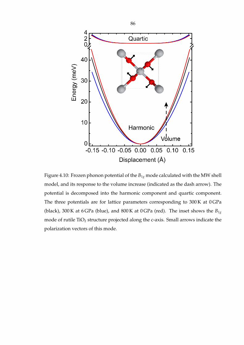
86
Figure 4.10: Frozen phonon potential of the B1g mode calculated with the MW shell
model, and its response to the volume increase (indicated as the dash arrow). The
potential is decomposed into the harmonic component and quartic component.
The three potentials are for lattice parameters corresponding to 300 K at 0 GPa
(black), 300 K at 6 GPa (blue), and 800 K at 0 GPa (red). The inset shows the B1g
mode of rutile TiO2 structure projected along the c-axis. Small arrows indicate the
polarization vectors of this mode.
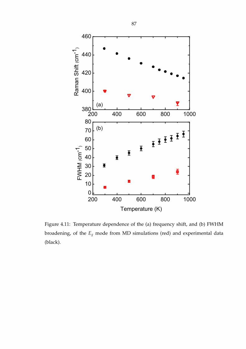
87
200 400 600 800 1000380
400
420
440
460
(a)
Ra
ma
n S
hift
(cm
-1)
(b)
200 400 600 800 1000
0
10
20
30
40
50
60
70
80
FW
HM
(cm
-1)
Temperature (K)
Figure 4.11: Temperature dependence of the (a) frequency shift, and (b) FWHM
broadening, of the Eg mode from MD simulations (red) and experimental data
(black).
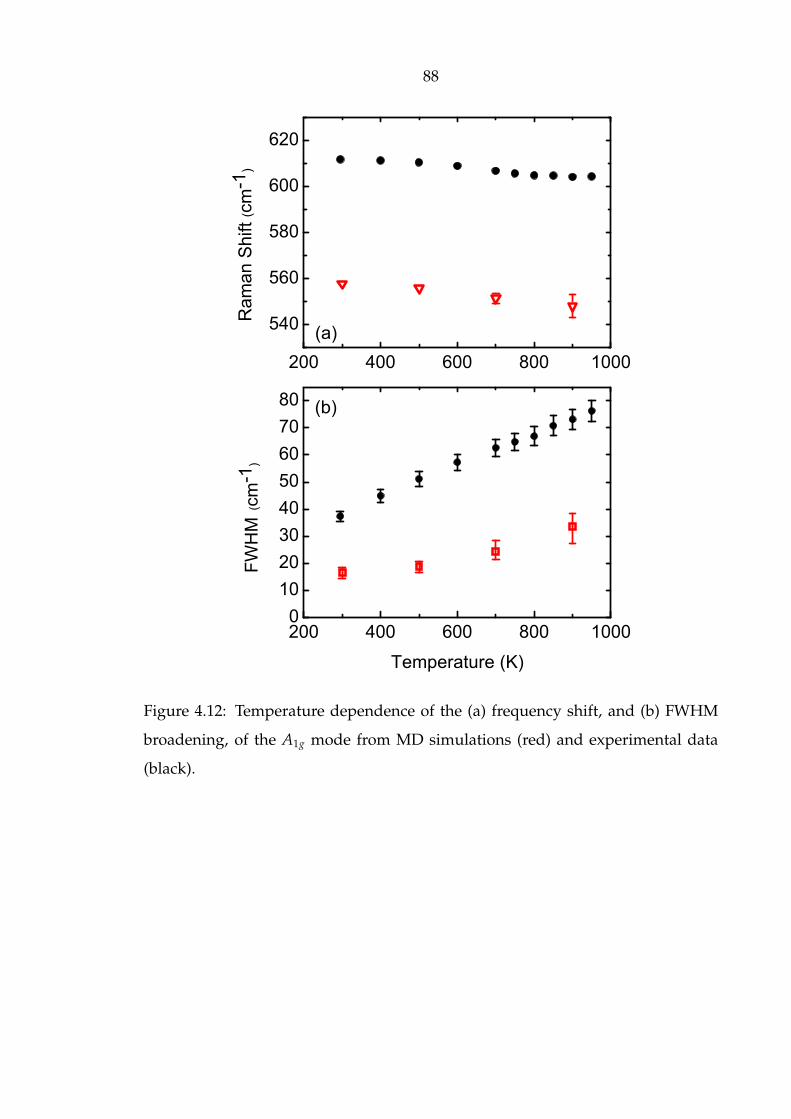
88
200 400 600 800 1000
540
560
580
600
620
(a)
Ra
ma
n S
hift
(cm
-1)
(b)
200 400 600 800 10000
10
20
30
40
50
60
70
80
FW
HM
(cm
-1)
Temperature (K)
Figure 4.12: Temperature dependence of the (a) frequency shift, and (b) FWHM
broadening, of the A1g mode from MD simulations (red) and experimental data
(black).

89
300 400 500 600 700 800 900 1000
0.0000.0030.006
0.02
0.04
0.06
0.08
0.10
0.12
0.14
0.16
Eg quarticA1g quartic
A1g cubic
Fra
ctio
n o
f H
arm
on
ic
Temperature (K)
B1g quartic
Figure 4.13: Ratio of the mode anharmonic potential and harmonic potential, with
increasing temperature.
4.6.3 Vibrational Entropy of Rutile TiO2
Vibrational entropy is important for thermophysical properties of materials, and
for the thermodynamic stabilities of different solid phases as reviewed recently [93].
The vibrational entropy Svib is
Svib = 3kB
∫ ∞
0g(ϵ)
[(n(ϵ) + 1) ln(n(ϵ) + 1) − n(ϵ) ln(n(ϵ))
]dϵ (4.13)
where g(ϵ) is the single phonon DOS at the temperature of interest, and n(ϵ) is the
phonon occupancy. Although Eq. 4.13 is derived from the harmonic model, it is
known to be valid for anharmonic systems to first order in perturbation theory [94].
From the phonon DOS obtained by MD simulations at elevated temperatures, Svib
was calculated with Eq. 4.13 and the results are presented in Table 4.4. The
calculated results are in general agreement with the experimental data, but the dis-

90
crepancies suggest that the average phonon frequencies from the MD calculations
are about 3.7 % too small.
Table 4.4: Entropy in J/(mol K) of rutile TiO2 from MD calculations and experimental
data of Ref. [95].
T [K] MD Experimental
300 48.01 50.69
500 80.28 82.21
700 101.79 105.51
900 119.22 123.65
4.7 Conclusions
Raman spectra were measured on rutile TiO2 at temperatures to 1150 K, and giant
anharmonic behaviors were found for the shifts and broadenings of the three mea-
surable Raman peaks. The pressure-dependence and temperature-dependence of
the Raman peak shifts were used to separate the anharmonic behavior from the
quasiharmonic behavior. Individual assessments of the cubic and quartic contribu-
tions to the anharmonicity were performed with a new data fitting method based
on the kinematics of 3-phonon and 4-phonon processes, with the phonons calcu-
lated from a shell model in this case. In fitting the anharmonic behavior, mode
broadening is from effects of cubic anharmonicity, while the anharmonic shifts are
from the same cubic factor plus a quartic anharmonicity. The quartic anharmonic-
ity of the B1g mode was found to be large, and its cubic anharmonicity small, unlike
the large cubic anharmonicity found for the Eg and A1g modes. From successes of
the fitting method, we suggest that the observed anharmonic effects are dominated
by considerations of the kinematics of energy and momentum conservation in the
phonon-phonon scattering processes, and less by the details of the anharmonicity
tensor.
Force field molecular dynamics (MD) calculations were performed with the
91
same shell model. Both the anomalous quasiharmonic behavior and the explicit
anharmonic behavior of the B1g mode from our calculations were in excellent
agreement with the experimental observation. No orthorhombic distortion was
found, suggesting that the anomalous anharmonicity originates with the phonon
responses to temperature and pressure, and not an incipient phase transition. Dis-
crepancies for the Eg and A1g modes suggest that the shell model potential may
not be sufficient for obtaining accurate anharmonicities from molecular dynamics
calculations, however.
92
Chapter 5
Phonon Anharmonicity of RutileSnO2
The main content of this chapter appeared in the journal article: Tian Lan, Chen W.
Li and Brent Fultz, Physical Review B 86, 134302 (2012).
93
Raman spectra of rutile tin dioxide (SnO2) were measured at temperatures from
83 to 873 K. The pure anharmonicity from phonon-phonon interactions was found
to be large and comparable to the quasiharmonicity. First principles calculations of
phonon dispersions were used to assess the kinematics of 3-phonon and 4-phonon
processes. These kinematics were used to generate Raman peak widths and shifts,
which were fit to measured data to obtain the cubic and quartic components of the
anharmonicity for each Raman mode. The B2g mode had a large quartic component,
consistent with the symmetry of its atom displacements. The broadening of the
B2g mode with temperature showed an unusual concave downwards curvature.
This curvature is caused by a change with temperature in the number of down-
conversion decay channels, originating with the wide band gap in the phonon
dispersions.
5.1 Introduction
Rutile tin dioxide (SnO2) is the most common and stable oxide of tin found in nature.
Owing to the wide variety of its applications for optoelectronics, heterogeneous
catalysis and gas sensors, rutile SnO2 has been the subject of much recent research.
[96] Lattice dynamics, phase transitions, and nanostructures of SnO2 have been
studied by measurements of optical phonons with Raman, Brillouin or infrared
spectroscopy, [65, 97–100] and by computation with force field models or density
functional theory. [97, 101–105] Rutile SnO2 is tetragonal with the space group
P4/mnm. The modes of symmetry B1g, Eg, A1g and B2g are Raman active, and
comprise motions of oxygen anions with respect to stationary tin cations, either
perpendicular to the c axis (modes B1g, A1g and B2g), or along the c axis (mode Eg).
Nonharmonic effects are known to be important for understanding the ther-
modynamic stability and the thermal transport properties of materials at elevated
temperatures, but the anharmonic lattice dynamics of rutile SnO2 is largely un-
known. Perhaps the most complete experimental results are from Peercy and
Morosin’s work in 1973. [65] They reported frequency shifts of Raman modes with

94
temperature and pressure, although the temperature range was below 480 K and
no phonon broadening information was reported. The linewidth broadening of the
A1g mode was measured to 973 K by Sato and Asari, and compared well with results
from shell model calculations. [102] Their results suggest that the anharmonicity
of SnO2 is large.
In our recent study on rutile TiO2, the pure anharmonicity gave shifts of Raman
peaks that were as large as from quasiharmonicity. [106] In that study we developed
a rigorous method of simultaneously fitting Raman peak widths and shifts with
calculations from the kinematics of phonon-phonon interactions. The effects of
cubic and quartic anharmonicity were separated, and these anharmonic effects
were found to be dominated by phonon kinematics. This previous work on TiO2
used kinematics calculated with a shell model, but in the present study on rutile
SnO2, inconsistencies in the different shell model parameters from the literature
motivated the use of ab initio methods to calculate phonon dispersions. The analysis
and comparison of our present results on rutile SnO2 with previous results on TiO2
provides a better understanding of the anharmonic phonon dynamics in both.
Figure 5.1: Rutile structure and oxygen atom displacements for Raman-active
modes.
95
Here we report high resolution measurements of Raman spectra at temper-
atures from 83 to 873 K. Both phonon frequency shifts and broadenings are re-
ported. The quasiharmonic effects from thermal expansion were separated from
the anharmonic effects of phonon-phonon interactions by comparing the tempera-
ture dependence to the pressure dependence of the Raman peaks. The data fitting
method used ab initio calculations of two-phonon kinematic functionals to identify
the effects of cubic and quartic anharmonicity. The peak broadening originates with
cubic anharmonicity, but the peak shifts depend on both cubic and quartic effects.
The phonon-phonon kinematics explains an unusual feature in the temperature
dependence of the broadening of the B2g mode of rutile SnO2. The large difference
in masses of Sn and O atoms causes a gap in the phonon density of states (DOS)
that produces a peak in the two-phonon DOS (TDOS). The thermal shift moves the
frequency of the B2g mode away from this peak in the TDOS, and reduces the num-
ber of channels available for three-phonon processes, giving a concave-downwards
curvature to the thermal broadening of the B2g peak. The symmetrical B2g mode
was found to have a relatively large quartic anharmonicity.
5.2 Experimental Procedures
Measurements were performed on both powder and single crystal samples of rutile
SnO2. The powder sample was prepared from commercial SnO2 powder (Alfa
Aesar, Ward Hill, MA) with a grain size of 10µm. The powder was compressed
into pellets of 1 mm thickness using a pressure of 50 MPa at ambient temperature.
Raman spectra were acquired before and after compression into a pellet, and were
found to be identical. A sample of single crystal casiterite of high optical quality
was provided by the Mineral Museum of the Division of Geological and Planetary
Sciences at the California Institute of Technology. The sample was cut and polished
to a thickness of approximately 0.3 mm. Samples were mounted on the silver block
of a Linkam thermal stage that provided excellent heat transfer and temperature
stability for both heating and cooling. The sample chamber was sealed and purged

96
with nitrogen gas flow. A temperature controller drove a 200 W power supply
for heating. For low temperature measurements, the stage was equipped with a
coolant pump that injected liquid nitrogen directly into the silver block. Samples
of powder pellets were measured at temperatures from 83 to 833 K, and the single
crystal sample was measured from 83 to 873 K. Each temperature was held stable
for 10 min before the spectrum was taken. The temperature precision was within
1 K.
The Raman spectra were measured with a Renishaw micro-Raman system with
an Olympus LMPlanFI microscope lens. The spectrometer was configured in
backscattering geometry, minimizing issues with the thickness of the sample. A
depolarized solid state laser operated at wavelength of 514.5 nm excited the sample
with the low incident power of 10 mW to avoid additional thermal heating. The
laser spot size was 12µm in diameter. To test for heating effects this spot size was
varied, but no changes were found. Each Raman spectrum was accumulated in 10
measurements with 10 s exposure times.
5.3 Results
Representative Raman spectra of powder samples are shown in Fig. 5.2. Three of
the four Raman-active modes, Eg, A1g and B2g, have enough intensity for extracting
quantitative information on phonon frequencies and linewidths. The B1g mode
was too weak for obtaining quantitative information (its intensity is about three
orders of magnitude smaller than that of the A1g mode [97]). The single crystal
sample showed very similar spectra, but the Eg mode was weaker primarily because
of orientation effects. Three weak abnormal Raman bands that were previously
reported [107] were also observed at 503, 545 and 692 cm−1 for both powder and
single crystal samples.
After background subtraction, each peak in each spectrum was fitted to a
Lorentzian function to obtain a centroid and full-width-at-half-maximum (FWHM).
The FWHM data from the experiment were corrected for the finite resolution of the
97
spectrometer. [81] At room temperature, the Raman peak frequencies were 475 cm−1
for Eg, 633 cm−1 for A1g, 774 cm−1 for B2g. The mode frequencies at 83 K, ω(83 K),
were 476 cm−1, 636 cm−1 and 778 cm−1. Figure 5.3 presents results of peak shifts and
widths versus temperature. Here the peak shift∆ω is defined asω(T)−ω(83 K). We
find good agreement with the frequency shift data reported by Peercy and Morosin
at temperatures below 480 K. [65] We also find good agreement with the linewidth
broadening data of the A1g mode reported by Sato and Asari to 900 K. [102]
With increasing temperature, the A1g and B2g modes undergo large shifts to
lower frequencies and significant linewidth broadenings, but the Eg mode under-
goes less shift and broadening. At high temperatures above 500 K, the broadening
of the B2g mode shows an unusual concave downward curvature, while the other
two modes broaden linearly. At low temperatures, the B2g mode has a much larger
linewidth than the other two modes. The linewidth of the B2g mode extrapolated
to 0 K is approximately 8 cm−1, whereas the linewidths of the Eg and A1g modes
extrapolate to less than 2 cm−1.
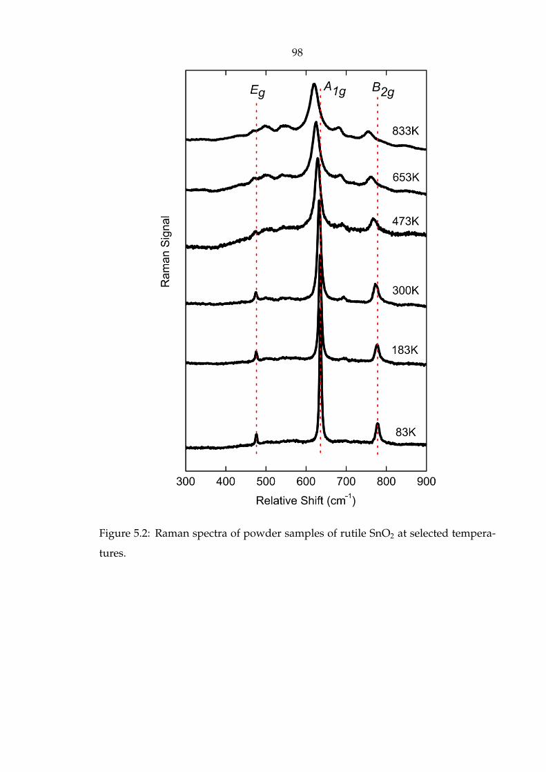
98
Figure 5.2: Raman spectra of powder samples of rutile SnO2 at selected tempera-
tures.
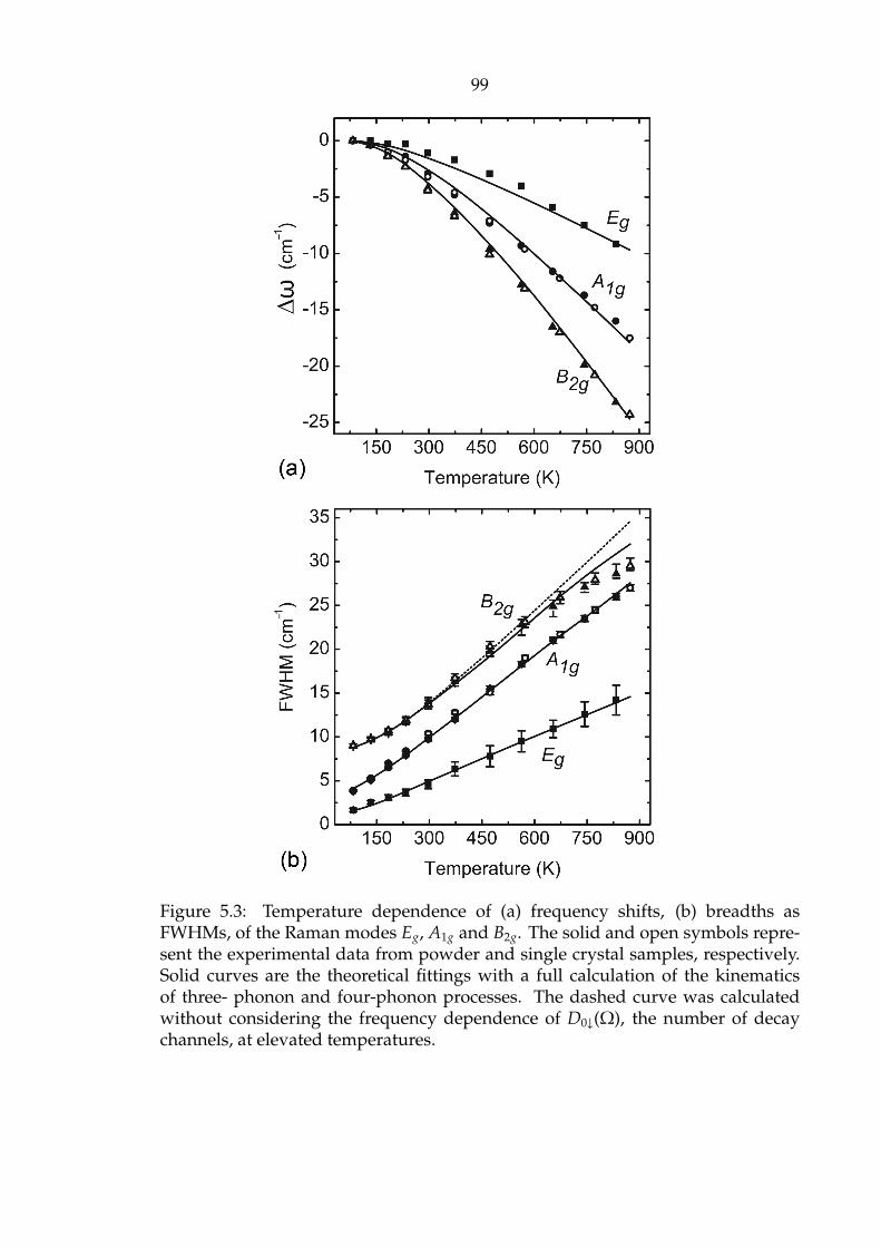
99
Figure 5.3: Temperature dependence of (a) frequency shifts, (b) breadths asFWHMs, of the Raman modes Eg, A1g and B2g. The solid and open symbols repre-sent the experimental data from powder and single crystal samples, respectively.Solid curves are the theoretical fittings with a full calculation of the kinematicsof three- phonon and four-phonon processes. The dashed curve was calculatedwithout considering the frequency dependence of D0↓(Ω), the number of decaychannels, at elevated temperatures.
100
5.4 Calculations
5.4.1 First Principles Lattice Dynamics
Phonon dispersion calculations over the whole Brillouin zone were performed
with the QuantumEspresso package, within the framework of ab initio density
functional perturbation theory (DFPT). [39] Vanderbilt ultrasoft pseudopotentials
with the local density approximation (LDA) and nonlinear core corrections were
used. The LO /TO splitting was corrected by adding a non-analytical part into the
dynamical matrix. [40] The calculated dispersion curves are shown in Fig. 6.2a,
and mode frequencies at the Γ-point are presented in Table 6.1. Calculations of
the phonon density of states (DOS) with a uniform 16×16×16 sampling grid were
also performed, as shown in Fig. 6.2b. Our calculations are in good agreement
with prior experimental and theoretical results. [97, 101–105] A band gap of width
100 cm−1, centered around 400 cm−1, is evident in Fig. 6.2. Above the gap, phonon
modes are dominated by the motions of oxygen atoms.
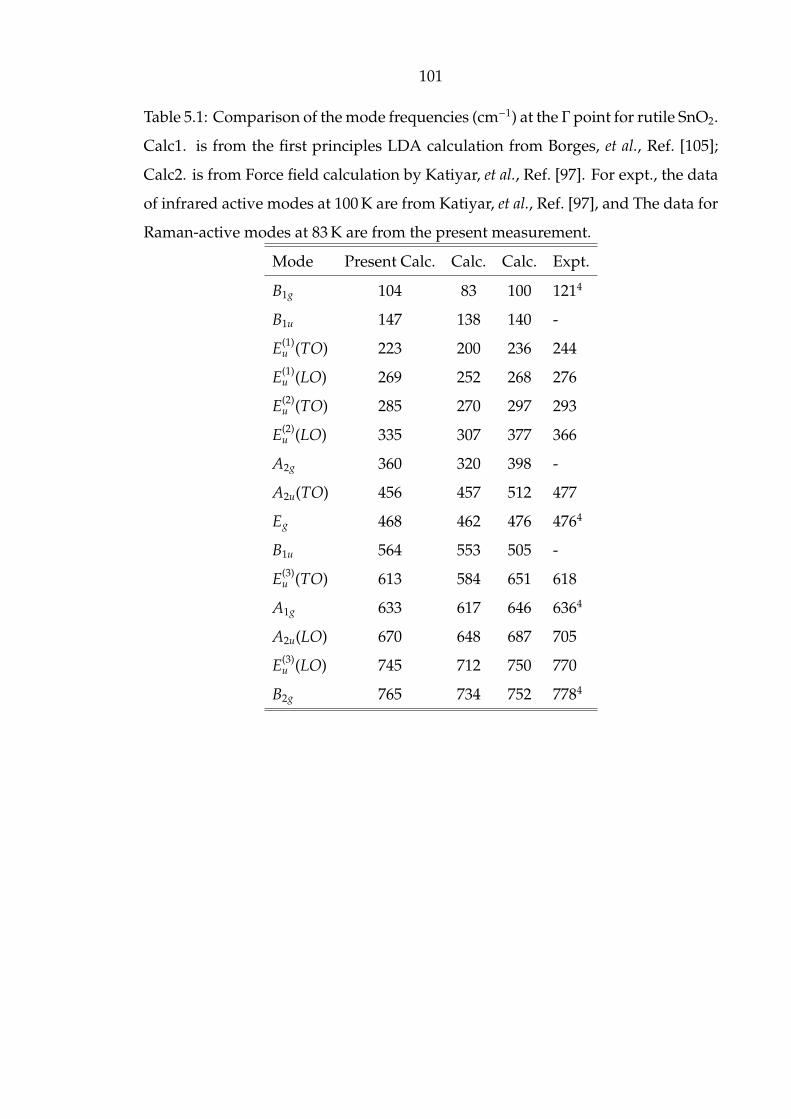
101
Table 5.1: Comparison of the mode frequencies (cm−1) at the Γ point for rutile SnO2.
Calc1. is from the first principles LDA calculation from Borges, et al., Ref. [105];
Calc2. is from Force field calculation by Katiyar, et al., Ref. [97]. For expt., the data
of infrared active modes at 100 K are from Katiyar, et al., Ref. [97], and The data for
Raman-active modes at 83 K are from the present measurement.
Mode Present Calc. Calc. Calc. Expt.
B1g 104 83 100 1214
B1u 147 138 140 -
E(1)u (TO) 223 200 236 244
E(1)u (LO) 269 252 268 276
E(2)u (TO) 285 270 297 293
E(2)u (LO) 335 307 377 366
A2g 360 320 398 -
A2u(TO) 456 457 512 477
Eg 468 462 476 4764
B1u 564 553 505 -
E(3)u (TO) 613 584 651 618
A1g 633 617 646 6364
A2u(LO) 670 648 687 705
E(3)u (LO) 745 712 750 770
B2g 765 734 752 7784

102
ARZX MГ Г
(b) DOS (a) Dispersions
0
100
200
300
400
500
600
700
800
Fre
qu
en
cy (
cm
-1)
Figure 5.4: (a) Calculated phonon dispersion along high symmetry directions
of rutile SnO2. Γ (0, 0, 0), X (0.5, 0, 0), M (0.5, 0.5, 0), Z (0, 0, 0.5), R (0.5, 0, 0.5) and
A (0.5, 0.5, 0.5). At the Γ point, the frequencies from Table 6.1 are presented as up
triangles (Raman) and down triangles (infrared). At the X, M, Z, R and A points,
the mode frequencies from Ref. [ [103]] (all doubly degenerate) are presented as
squares. (b) Total phonon DOS (black curve) and oxygen-projected DOS (filled
green).
5.4.2 The Kinematic Functionals Dω(Ω) and Pω(Ω)
In anharmonic phonon perturbation theory, [2] the phonon linewidth is related to
the two-phonon density of states (TDOS), D(Ω), which is defined as
D(Ω) =∑q1, j1
∑q2 j2
D(Ω,ω1,ω2)
=1N
∑q1, j1
∑q2, j2
∆(q1 + q2)[(n1 + n2 + 1) δ(Ω − ω1 − ω2)
+ 2(n1 − n2) δ(Ω+ ω1 − ω2)]
(5.1)
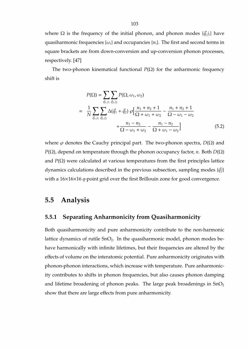
103
where Ω is the frequency of the initial phonon, and phonon modes qi ji have
quasiharmonic frequencies ωi and occupancies ni. The first and second terms in
square brackets are from down-conversion and up-conversion phonon processes,
respectively. [47]
The two-phonon kinematical functional P(Ω) for the anharmonic frequency
shift is
P(Ω) =∑q1, j1
∑q2, j2
P(Ω,ω1,ω2)
=1N
∑q1, j1
∑q2, j2
∆(q1 + q2) ℘[ n1 + n2 + 1Ω+ ω1 + ω2
− n1 + n2 + 1Ω − ω1 − ω2
+n1 − n2
Ω − ω1 + ω2− n1 − n2
Ω+ ω1 − ω2
](5.2)
where ℘ denotes the Cauchy principal part. The two-phonon spectra, D(Ω) and
P(Ω), depend on temperature through the phonon occupancy factor, n. Both D(Ω)
and P(Ω) were calculated at various temperatures from the first principles lattice
dynamics calculations described in the previous subsection, sampling modes q jwith a 16×16×16 q-point grid over the first Brillouin zone for good convergence.
5.5 Analysis
5.5.1 Separating Anharmonicity from Quasiharmonicity
Both quasiharmonicity and pure anharmonicity contribute to the non-harmonic
lattice dynamics of rutile SnO2. In the quasiharmonic model, phonon modes be-
have harmonically with infinite lifetimes, but their frequencies are altered by the
effects of volume on the interatomic potential. Pure anharmonicity originates with
phonon-phonon interactions, which increase with temperature. Pure anharmonic-
ity contributes to shifts in phonon frequencies, but also causes phonon damping
and lifetime broadening of phonon peaks. The large peak broadenings in SnO2
show that there are large effects from pure anharmonicity.
104
To separate the peak shifts caused by pure anharmonicity from shifts caused
by quasiharmonicity, we treat the mode frequency ω j = ω j(V,T) as a function of
volume and temperature [59](∂ lnω j
∂T
)P= −β
κ
(∂ lnω j
∂P
)T+
(∂ lnω j
∂T
)V
(5.3)
where j is the phonon mode index, β is the volume thermal expansivity and κ
is the isothermal compressibility. This is a general method to separate phonon
quasiharmonicity from phonon anharmonicity, and is not unique for rutile struc-
tures, for example. The left-hand side gives the directly measurable temperature-
dependent isobaric frequency shift, including both quasiharmonic and pure anhar-
monic behavior. The first term on the right-hand side, the isothermal frequency
shift as a function of pressure, is the quasiharmonic contribution, which is also
measureable. By defining a mode Gruneisen parameter as the proportionality of
the relative change of the mode frequency to the relative change of volume, i.e.,
γ j = −∂(lnω j)/(∂(ln V)), the quasiharmonic term can be written as γ jβ. The second
term on the right of Eq. 6.7 is the frequency shift from the pure anharmonicity,
which depends on temperature and not volume. From the difference of the iso-
baric and isothermal frequency shifts, the pure anharmonicity can be determined
experimentally.
To obtain the quasiharmonic contributions to the peak shifts, we used the mode
Gruneisen parameters γ j reported recently by Hellwig, et al., from Raman mea-
surements at pressures to 14 GPa, [98] which agreed well with earlier high pressure
measurements to 4 GPa. [108] These results suggest that Peercy and Morosin over-
estimated the quasiharmonic contributions to their data, for which the pressure
was only 0.4 GPa.
We also performed first principles calculations of the mode Gruneisen parame-
ters by optimizing the enthalpy function to 10 GPa. Our calculated γ j were in good
agreement with the experimental results of Hellwig, et al., and both are listed in
Table 5.2. Since the γ j are very weakly dependent on temperature, as is the thermal

105
Table 5.2: Frequencies of the three Raman modes, mode Gruneisen parameters,and the logarithmic pressure and temperature derivatives of frequency. Gruneisenparameters data from Hellwig, et al., Ref. [98]. Thermal expansion data from Peercyand Morosin, Ref. [65]
ω(300 K) γ j γ j
(∂ lnω∂T
)P= −γ jβ +
(∂ lnω∂T
)V
Mode (cm−1) [expt.] [calc.] (10−5K−1) (10−5K−1) (10−5K−1)Eg 475 1.45 1.48 -2.6 -1.7 -0.9A1g 633 1.65 1.81 -4.2 -1.9 -2.3B2g 774 1.49 1.71 -4.6 -1.7 -2.9
expansion above 400 K, [59, 65] the γ j were assumed to be constants when assess-
ing the volume dependent quasiharmonic contribution. The last two columns of
Table 5.2 separate the measured isobaric temperature derivatives into the pure
volume and pure temperature contributions as in Eq. 6.7. These last columns in
Table 5.2 are the frequency shifts from quasiharmonicity and pure anharmonicity
at temperatures above 400 K.
By comparing the last two columns in Table 5.2, we see that like rutile TiO2, the
pure anharmonic contribution is comparable to the quasiharmonic contribution
above 400 K. Nevertheless, the total anharmonicity of SnO2 is considerably smaller
than for TiO2. For the modes A1g and B2g in SnO2, the pure anharmonic contribution
is larger than the quasiharmonic, while the Eg mode is more quasiharmonic. The
relative magnitudes of pure anharmonicities of the three modes derived from
the frequency shift data are consistent with the relative magnitudes of linewidth
broadenings of the modes as shown in Fig. 5.3b.
5.5.2 Cubic and Quartic Anharmonicity
Anharmonicity tensors describe the coupling strengths for phonon-phonon inter-
actions, but a prerequisite is that the phonons in these processes satisfy the kine-
matical conditions of conservation of energy and momentum. An anharmonicity

106
tensor element for an s-phonon process is [46]
V( j; q1 j1; ...; qs−1 js−1) =1
2s!
(~
2N
) s2
N∆(q1 + · · · + qs−1)
×[ω j0ω1 · · · ωs−1 ]12 C( j; q1 j1; ...; qs−1 js−1) (5.4)
where ∆(q1 + · · · + qs−1) enforces momentum conservation and the C(.)’s, elements
of the s-phonon anharmonic tensor, are expected to be slowly-varying functions of
their arguments. The cubic anharmonicity tensor has been calculated by first prin-
ciples methods, [47, 109, 110] but to our knowledge the the quartic anharmonicity
tensor has never been fully calculated from first principles.
Nevertheless, if the anharmonicity tensor or its average does not vary signifi-
cantly for different phonon processes, the coupling factor and the kinematic factor
are approximately separable in Eq. 6.2. The separation of the anharmonic cou-
pling and the kinematics has been used with success in many studies including
our recent report on rutile TiO2. [106] We consider the term C( j; q1 j1; ...; qs−1 js−1) to
be a constant of the Raman mode j, and use it as a fitting parameter. Although
C( j; q1 j1; q2 j2) and C( j; j; q1 j1;−q1 j1) change with j1 and j2, an average over modes,
⟨C(.)⟩ = ∑1,2 C( j; q1 j1; q2 j2)/
∑1,2 1, is needed by the fitting, where 1, 2 under the sum-
mation symbol represent qi ji. We define the cubic and quartic fitting parameters as
C(3)j = ⟨C( j; q1 j1; q2 j2)⟩ (5.5a)
C(4)j = ⟨C( j; j; q1 j1;−q1 j1)⟩ (5.5b)
To the leading order of cubic and quartic anharmonicity, the broadening of the
Raman peaks is 2Γ(3)( j;Ω). The frequency shift of the Raman peaks is ∆Q + ∆(3) +
∆(3′) +∆(4), where the quasiharmonic part ∆Q is the integral form of the first term in
Eq. 6.7. These quantities can be written as functions of D(Ω,ω1,ω2) and P(Ω,ω1,ω2),
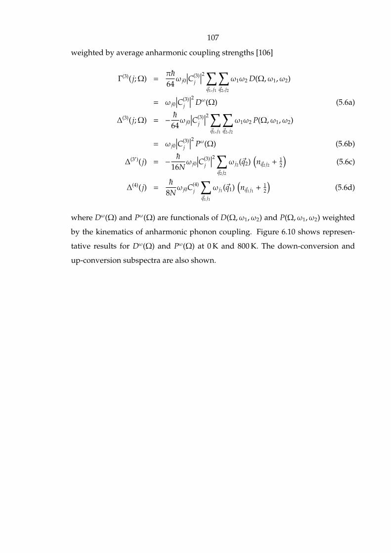
107
weighted by average anharmonic coupling strengths [106]
Γ(3)( j;Ω) =π~64ω j0
∣∣∣C(3)j
∣∣∣2 ∑q1, j1
∑q2, j2
ω1ω2 D(Ω,ω1,ω2)
= ω j0
∣∣∣C(3)j
∣∣∣2 Dω(Ω) (5.6a)
∆(3)( j;Ω) = − ~64ω j0
∣∣∣C(3)j
∣∣∣2 ∑q1, j1
∑q2, j2
ω1ω2 P(Ω,ω1,ω2)
= ω j0
∣∣∣C(3)j
∣∣∣2 Pω(Ω) (5.6b)
∆(3′)( j) = − ~16Nω j0
∣∣∣C(3)j
∣∣∣2 ∑q2 j2
ω j2(q2)(nq2 j2 +
12
)(5.6c)
∆(4)( j) =~
8Nω j0C(4)
j
∑q1 j1
ω j1(q1)(nq1 j1 +
12
)(5.6d)
where Dω(Ω) and Pω(Ω) are functionals of D(Ω,ω1,ω2) and P(Ω,ω1,ω2) weighted
by the kinematics of anharmonic phonon coupling. Figure 6.10 shows represen-
tative results for Dω(Ω) and Pω(Ω) at 0 K and 800 K. The down-conversion and
up-conversion subspectra are also shown.
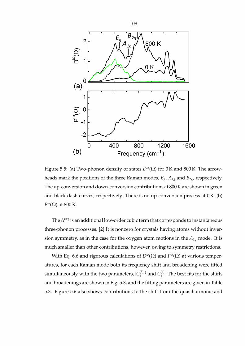
108
Figure 5.5: (a) Two-phonon density of states Dω(Ω) for 0 K and 800 K. The arrow-
heads mark the positions of the three Raman modes, Eg, A1g and B2g, respectively.
The up-conversion and down-conversion contributions at 800 K are shown in green
and black dash curves, respectively. There is no up-conversion process at 0 K. (b)
Pω(Ω) at 800 K.
The∆(3′) is an additional low-order cubic term that corresponds to instantaneous
three-phonon processes. [2] It is nonzero for crystals having atoms without inver-
sion symmetry, as in the case for the oxygen atom motions in the A1g mode. It is
much smaller than other contributions, however, owing to symmetry restrictions.
With Eq. 6.6 and rigorous calculations of Dω(Ω) and Pω(Ω) at various temper-
atures, for each Raman mode both its frequency shift and broadening were fitted
simultaneously with the two parameters, |C(3)j |2 and C(4)
j . The best fits for the shifts
and broadenings are shown in Fig. 5.3, and the fitting parameters are given in Table
5.3. Figure 5.6 also shows contributions to the shift from the quasiharmonic and
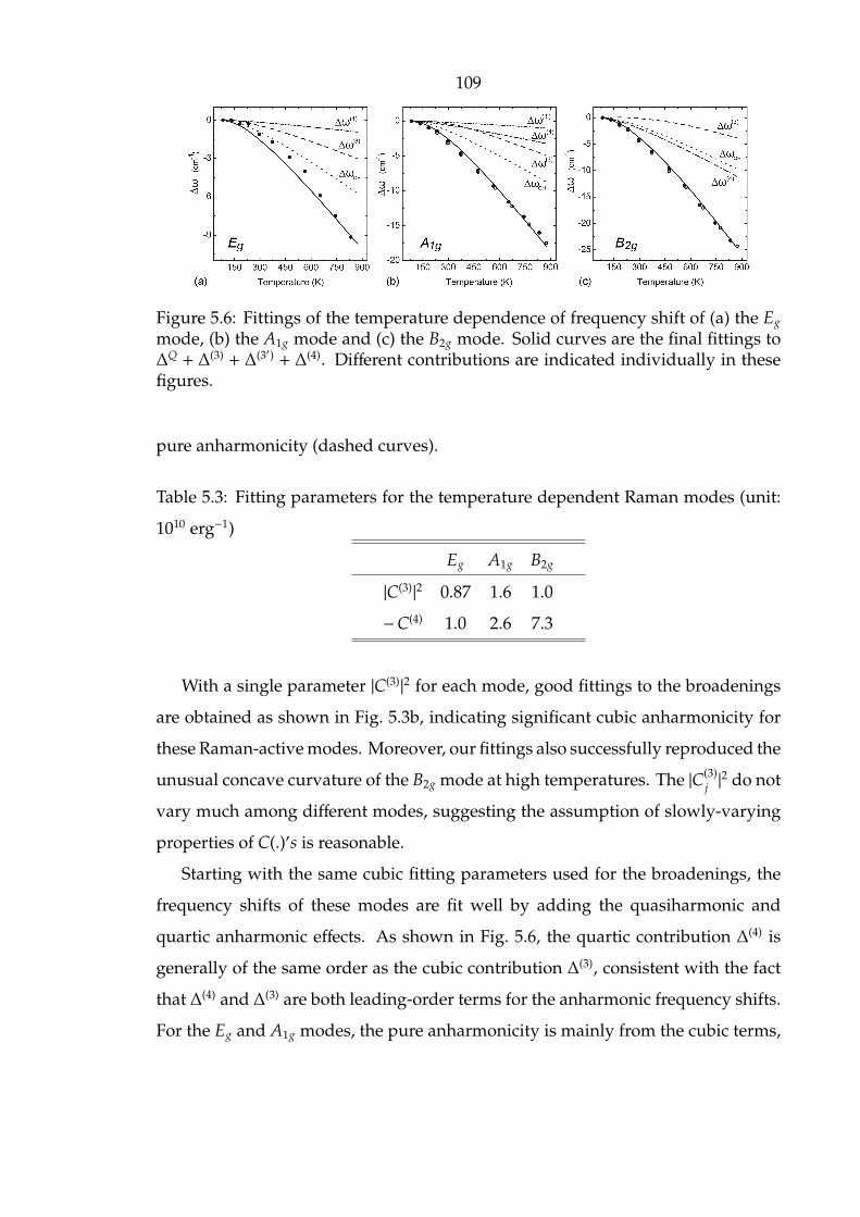
109
Figure 5.6: Fittings of the temperature dependence of frequency shift of (a) the Eg
mode, (b) the A1g mode and (c) the B2g mode. Solid curves are the final fittings to∆Q + ∆(3) + ∆(3′) + ∆(4). Different contributions are indicated individually in thesefigures.
pure anharmonicity (dashed curves).
Table 5.3: Fitting parameters for the temperature dependent Raman modes (unit:
1010 erg−1)
Eg A1g B2g
|C(3)|2 0.87 1.6 1.0
−C(4) 1.0 2.6 7.3
With a single parameter |C(3)|2 for each mode, good fittings to the broadenings
are obtained as shown in Fig. 5.3b, indicating significant cubic anharmonicity for
these Raman-active modes. Moreover, our fittings also successfully reproduced the
unusual concave curvature of the B2g mode at high temperatures. The |C(3)j |2 do not
vary much among different modes, suggesting the assumption of slowly-varying
properties of C(.)′s is reasonable.
Starting with the same cubic fitting parameters used for the broadenings, the
frequency shifts of these modes are fit well by adding the quasiharmonic and
quartic anharmonic effects. As shown in Fig. 5.6, the quartic contribution ∆(4) is
generally of the same order as the cubic contribution ∆(3), consistent with the fact
that ∆(4) and ∆(3) are both leading-order terms for the anharmonic frequency shifts.
For the Eg and A1g modes, the pure anharmonicity is mainly from the cubic terms,
110
but for the B2g mode, the quartic anharmonicity is dominant and is as large as the
quasiharmonic part.
5.6 Discussion
We can understand why the B2g mode has a relatively larger quartic anharmonicity
than the A1g from differences in how the O atoms move towards the Sn atoms.
Using a unit cell with 4 O atoms and 2 Sn atoms, as shown in Fig. 5.1, the A1g mode
has all 4 O atoms moving directly into one Sn atom on one half of the cycle, but
moving between two Sn atoms during the other half cycle. The B2g mode has 2 O
atoms moving into a Sn atom and 2 O atoms moving between two Sn atoms on both
halves of the vibrational cycle, making for a potential that is an even function of the
phonon coordinate. Table 5.3 shows a larger quartic contribution for the B2g mode
than the A1g. (The Eg mode does not have similar atom motions for comparison.)
The TDOS function Dω(Ω) in Fig. 6.10 shows large variations with Ω that ex-
plains a trend in the thermal broadening of Fig. 5.3b. Owing to the high frequency
of the B2g mode, at the temperatures of this study its phonon-phonon anharmonic-
ity comes mostly from down-conversion processes, as shown in Fig. 6.10. Ignoring
the small up-conversion contribution, at high temperatures [48]
Dω(Ω,T) ∝ T∑q1, j1
∑q2, j2
δ(Ω − ω1 − ω2) ≡ T D0↓(Ω) (5.7)
where D0↓(Ω) is the number of two-phonon down-conversion channels. Usually the
line broadening is linear in T because D0↓(Ω) does not vary much with temperature.
However, the B2g mode at 774 cm−1 lies on a steep gradient of Dω(Ω,T) in Fig. 6.10.
Because the B2g mode undergoes a significant shift of frequency with temperature,
it moves down the gradient of Dω(Ω,T), and its broadening is less than linear
in T. The temperature dependence of the broadening of the B2g mode has an
unusual concave downwards shape. For comparison, the dashed line in Fig. 5.3
was calculated without considering the frequency dependence of D0↓(Ω) at elevated

111
temperatures, and it deviates substantially from the experimental trend.
The unusual temperature dependence of the linewidth of the B2g mode comes
from the sharp peak in Dω(Ω,T) centered at 800 cm−1. This feature in the TDOS
originates with the phonon DOS of SnO2 shown in Fig. 6.2, which has a band
gap between 360 cm−1 to 450 cm−1 associated with the mass difference of Sn and O
atoms. The shape of the TDOS can be understood as the convolution of the phonon
DOS with itself. With two approximately equal regions above and below the gap,
the result is a peak at 800 cm−1, with steep slopes on both sides. For comparison,
although the TDOS of rutile TiO2 is shaped as a broad peak, [106] it does not have
the sharp features of Fig. 6.10a because the mass difference between Ti and O atoms
does not cause a band gap in the phonon DOS of TiO2.
Especially with more up-conversion processes at higher temperatures, there is
another peak in the SnO2 TDOS at 400 cm−1. The up-conversion channels are pri-
marily from the pairs of sharp peaks in the phonon DOS at 100 cm−1 and 500 cm−1,
200 cm−1 and 600 cm−1, and 350 cm−1 and 750 cm−1. Although the Eg mode at
475 cm−1 is on the slope of this peak in the TDOS, the Eg mode does not show
anomalous broadening with temperature because it undergoes only a small ther-
mal shift in frequency.
In the low-temperature limit, up-conversion processes are prohibited because
n → 0. The peak linewidth extrapolated to 0 K is determined entirely by down-
conversion processes, quantified by the down-conversion TDOS. [48] The B2g mode
has a significant broadening because its frequency is near a peak in the down-
conversion TDOS, as seen in Fig. 6.10. On the other hand, the Eg and A1g modes are
not broadened at low temperatures because their frequencies are at low values of
the TDOS. The phonon-phonon kinematics accounts for the significant difference of
linewidths between the B2g and the other two Raman modes at low temperatures.

112
5.7 Conclusions
Raman spectra were measured on rutile SnO2 at temperatures from 83 to 873 K,
and large anharmonic shifts and broadenings were found for the three measurable
Raman peaks. Individual assessments of the cubic and quartic contributions to
the anharmonicity were performed by calculating the kinematics of 3-phonon and
4-phonon processes with ab initio methods, and varying the anharmonic coupling
parameters to fit the peak shifts and broadenings simultaneously. The quartic
anharmonicity of the B2g mode was found to be large, unlike the Eg and A1g modes
for which cubic anharmonicity is dominant. The quartic behavior of the B2g mode
can be understood from the symmetry of the oxygen atom displacements.
The phonon DOS of SnO2 has a band gap around 400 cm−1 owing to the mass
difference of Sn and O atoms, with similar structure above and below the gap. This
causes a sharp peak in the TDOS at 800 cm−1. The frequency of the B2g mode is on the
slope of this peak in the TDOS, and its frequency shift with temperature reduces the
number of down-conversion channels for its broadening. The thermal broadening
of the B2g mode consequently shows an anomalous concave downwards curvature.
At 0 K, the large TDOS around 800 cm−1 explains the large linewidth of the B2g
mode. The anharmonic peak shifts and broadenings were well accounted for by
the kinematics of phonon-phonon interactions, suggesting that on the average, the
anharmonicity tensors for rutile SnO2 are not rich in structure.

113
Chapter 6
Phonon Anharmonicity of Ag2O withCuprite Structure
The main content of this chapter appeared in the journal article: Tian Lan, Chen W.
Li, Jennifer L. Niedziela, Hillary Smith, Douglas L. Abernathy, George R. Rossman,
and Brent Fultz Physical Review B 89, 054306 (2014)
114
Inelastic neutron scattering measurements on silver oxide (Ag2O) with the
cuprite structure were performed at temperatures from 40 to 400 K, and Fourier
transform far-infrared spectra were measured from 100 to 300 K. The measured
phonon densities of states and the infrared spectra showed unusually large en-
ergy shifts with temperature, and large linewidth broadenings. First principles
molecular dynamics (MD) calculations were performed at various temperatures,
successfully accounting for the negative thermal expansion (NTE) and local dy-
namics. Using the Fourier-transformed velocity autocorrelation method, the MD
calculations reproduced the large anharmonic effects of Ag2O, and were in excel-
lent agreement with the neutron scattering data. The quasiharmonic approximation
(QHA) was less successful in accounting for much of the phonon behavior. The
QHA could account for some of the NTE below 250 K, although not at higher
temperatures. Strong anharmonic effects were found for both phonons and for the
NTE. The lifetime broadenings of Ag2O were explained by anharmonic perturba-
tion theory, which showed rich interactions between the Ag-dominated modes and
the O-dominated modes in both up- and down-conversion processes.
6.1 Introduction
Silver oxide (Ag2O) with the cuprite structure has attracted much interest after the
discovery of its extraordinarily large negative thermal expansion (NTE), [111, 112]
which exceeds −1 × 10⁻⁵ K−1 and occurs over a wide range of temperature from
40 K to its decomposition temperature near 500 K. Besides its large NTE, Ag2O is
commonly used as a modifier in fast-ion conducting glasses and batteries, [113,114]
and its catalytic properties are also of interest. [115, 116]
In the cuprite structure of Ag2O shown in Fig. 6.1, the fcc Ag lattice is expanded
by the presence of the O atoms, which form an interpenetrating bcc lattice. The O
atoms occupy two tetrahedral sites of the standard fcc unit cell of Ag atoms. Each O
atom is linked to four O atoms through a bridging Ag atom, placing the Ag atoms
in linear O-Ag-O links with little transverse constraint. A geometrical model of
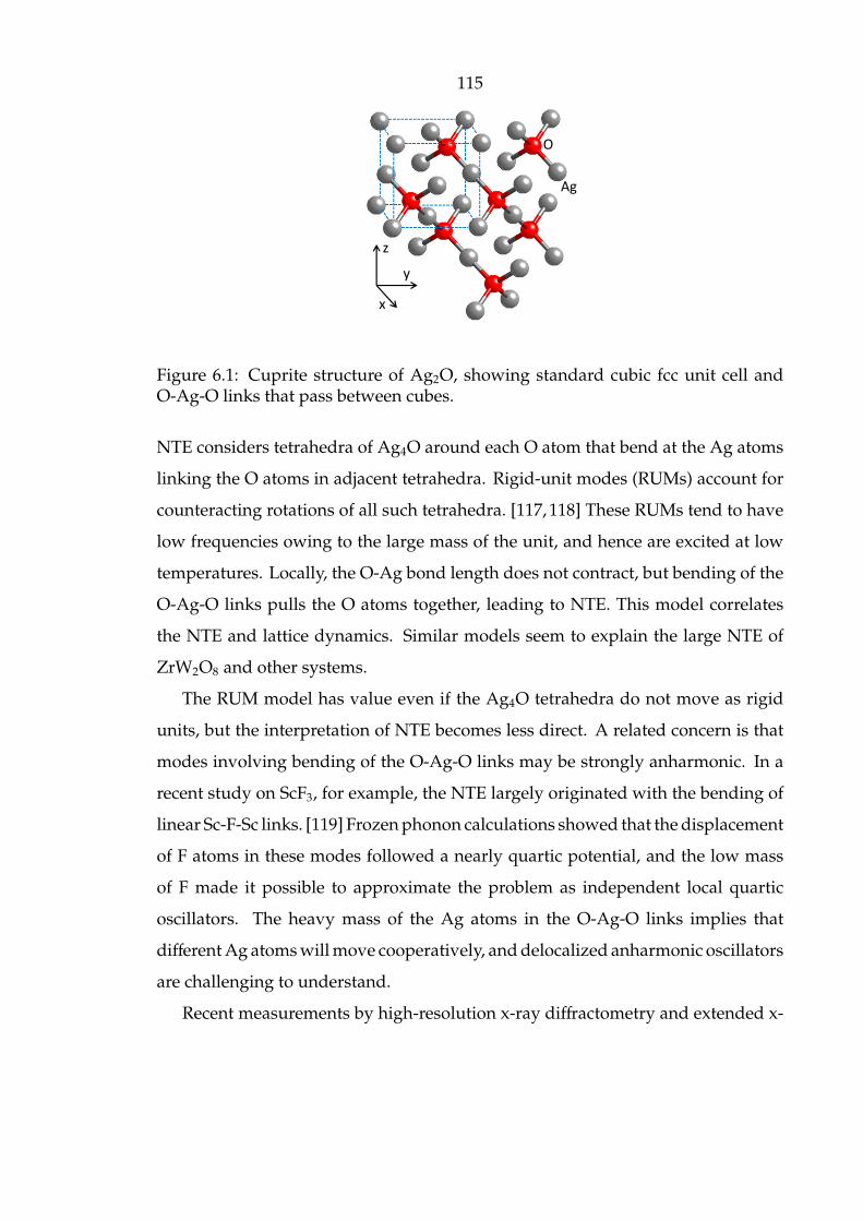
115
x
y
z
O
Ag
Figure 6.1: Cuprite structure of Ag2O, showing standard cubic fcc unit cell andO-Ag-O links that pass between cubes.
NTE considers tetrahedra of Ag4O around each O atom that bend at the Ag atoms
linking the O atoms in adjacent tetrahedra. Rigid-unit modes (RUMs) account for
counteracting rotations of all such tetrahedra. [117, 118] These RUMs tend to have
low frequencies owing to the large mass of the unit, and hence are excited at low
temperatures. Locally, the O-Ag bond length does not contract, but bending of the
O-Ag-O links pulls the O atoms together, leading to NTE. This model correlates
the NTE and lattice dynamics. Similar models seem to explain the large NTE of
ZrW2O8 and other systems.
The RUM model has value even if the Ag4O tetrahedra do not move as rigid
units, but the interpretation of NTE becomes less direct. A related concern is that
modes involving bending of the O-Ag-O links may be strongly anharmonic. In a
recent study on ScF3, for example, the NTE largely originated with the bending of
linear Sc-F-Sc links. [119] Frozen phonon calculations showed that the displacement
of F atoms in these modes followed a nearly quartic potential, and the low mass
of F made it possible to approximate the problem as independent local quartic
oscillators. The heavy mass of the Ag atoms in the O-Ag-O links implies that
different Ag atoms will move cooperatively, and delocalized anharmonic oscillators
are challenging to understand.
Recent measurements by high-resolution x-ray diffractometry and extended x-

116
ray absorption fine structure spectrometry (EXAFS) showed large deformations of
the Ag4O tetrahedra. [120–123] Although these tetrahedra are not distorted by a
pure RUM, the simultaneous excitation of other modes makes it unrealistic to view
the dynamics as motions of rigid framework units. Measurements by EXAFS also
showed that the average Ag-O nearest-neighbor distance expands slightly upon
heating, but the Ag-Ag next-nearest neighbor distance contracts approximately as
expected from the bulk NTE.
Anharmonic phonon behavior is known to be important for the thermody-
namics and the thermal conductivity of materials at elevated temperatures. It is
also important for the thermodynamic stability of phases. [124, 125] Anharmonic
phonon behavior is sometimes associated with NTE, but such relationships are not
well understood, and helped motivate the present study.
Inelastic neutron scattering is a powerful method to measure phonon dynamics,
allowing accurate measurements of vibrational entropy. [93] Additionally, phonon
energy broadening can be measured, allowing further assessment of how anhar-
monic effects originate from the non-quadratic parts of the interatomic potential.
A recent inelastic neutron scattering experiment on Ag2O with the cuprite struc-
ture showed phonon softening (reduction in energy) with temperature. [126] The
authors interpreted this result with a quasiharmonic model, where they calculated
harmonic phonons for reduced volumes of the structure and obtained a negative
Gruneissen parameter. These measurements were performed on the neutron en-
ergy gain side of the elastic line, restricting measurements to temperatures above
150 K, and the available energy range of 20 meV allowed about a quarter of the
Ag2O phonon spectrum to be measured.
Lattice dynamics calculations, based on either classical force fields or density
functional theory (DFT), have been used to study materials with the cuprite struc-
ture. [126–128] All these calculations were performed with the quasiharmonic ap-
proximation (QHA), where the interatomic forces and phonon frequencies changed
with volume, but all phonons were assumed to be harmonic normal modes with
infinite lifetimes. This QHA ignores interactions of phonons at finite temperatures

117
through the cubic or quartic parts of the interatomic potential, but these interac-
tions are essential to explicit phonon anharmonicity. Although the QHA calculation
accounted for the NTE behavior in ZrW2O8, [129] for Ag2O with the cuprite struc-
ture, the QHA was only partly successful. Molecular dynamics (MD) simulations
should be reliable for calculating phonon spectra in strongly anharmonic systems
, [72, 130, 131] even when the QHA fails. To our knowledge, no MD investigation
has yet been performed on Ag2O with the cuprite structure.
To study phonon anharmonicity in Ag2O, and its possible relationship to NTE,
we performed temperature-dependent inelastic neutron scattering experiments at
temperatures from 40 to 400 K to obtain the phonon density of states (DOS). (At
temperatures below 40 K a first-order phase transition occurs, giving a temperature-
dependent fraction of a second phase with different phonon properties [112, 132].)
Fourier transform infrared spectrometry at cryogenic temperatures was also used
to measure the frequencies and lineshapes of phonons at the Γ-point of the Bril-
louin zone. First-principles ab-initio MD simulations were performed, and by
Fourier transforming the velocity autocorrelation function, the large temperature-
dependent phonon anharmonicity was reproduced accurately. An independent
calculation of anharmonic phonon interaction channels was performed with in-
teracting phonon perturbation theory, and semiquantitatively explained anhar-
monicites of the different phonons. Most of the phonons have many channels for
decay and are highly anharmonic. Although the QHA is capable of predicting
about half of the NTE at low temperatures, part of this NTE is associated with
anharmonicity, and most of the NTE above 250 K originates with anharmonic in-
teractions between Ag-dominated and O-dominated phonon modes.
118
6.2 Experiments
6.2.1 Inelastic Neutron Scattering
Inelastic neutron scattering measurements were performed with the wide angular-
range chopper spectrometer, ARCS, [13] at the Spallation Neutron Source at Oak
Ridge National Laboratory. Powder samples of Ag2O with the cuprite structure of
99.99% purity were loaded into an annular volume between concentric aluminum
cylinders with an outer diameter of 29 mm and an inner diameter of 27 mm, giving
about 5% scattering of the incident neutron beam. The sample assembly was
mounted in a bottom-loading closed cycle refrigerator outfitted with a sapphire
hot stage that can be controlled independently of the second stage of the cryostat.
Spectra were acquired with two incident neutron energies of approximately 30
and 100 meV. Measurements were performed at temperatures of 40, 100, 200, 300
and 400 K, each with approximately 1.6 × 10⁶ neutron counts. Backgrounds with
empty sample cans were measured at each temperature. Ag has an absorption
cross section of 63 barns, but this was not be a problem with low background and
high neutron flux.
The raw data were rebinned into intensity I as a function of momentum transfer
Q and energy transfer E. After deleting the elastic peak around zero energy,
neutron-weighted phonon densities of states curves were calculated from I(Q, E) by
subtracting the measured background, and using an iterative procedure to remove
contributions from multiple scattering and higher-order multiphonon processes.
[133]
6.2.2 Fourier Transform Far-Infrared Spectrometer
The far-infrared spectrometry measurements were performed with a Thermo-
Nicolet Magna 860 FTIR spectrometer using a room-temperature deuterated triglycine
sulfate detector and a solid substrate beam splitter. The same Ag2O powder was
mixed with polyethylene fine powder with a mass ratio of 1:19 and finely ground.
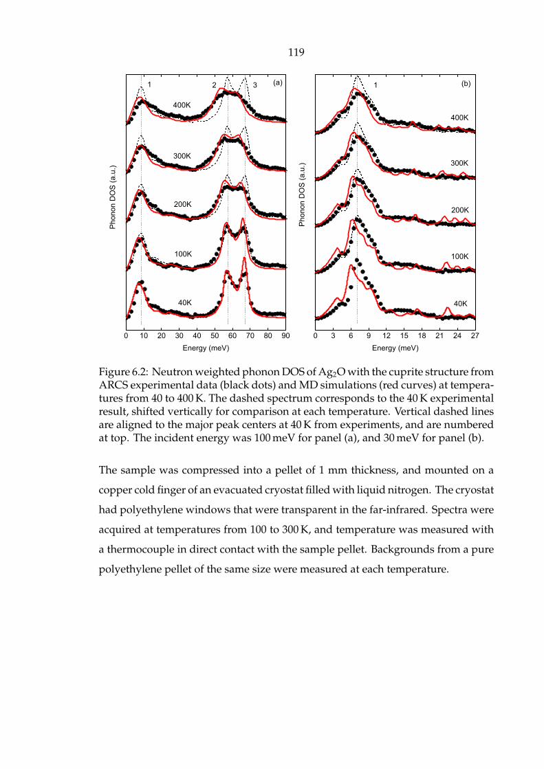
119
0 10 20 30 40 50 60 70 80 90
400K
300K
200K
100K
Ph
on
on
DO
S (
a.u
.)
Energy (meV)
40K
0 3 6 9 12 15 18 21 24 27
400K
300K
200K
100K
Ph
on
on
DO
S (
a.u
.)
Energy (meV)
40K
1 12 3 (a) (b)
Figure 6.2: Neutron weighted phonon DOS of Ag2O with the cuprite structure fromARCS experimental data (black dots) and MD simulations (red curves) at tempera-tures from 40 to 400 K. The dashed spectrum corresponds to the 40 K experimentalresult, shifted vertically for comparison at each temperature. Vertical dashed linesare aligned to the major peak centers at 40 K from experiments, and are numberedat top. The incident energy was 100 meV for panel (a), and 30 meV for panel (b).
The sample was compressed into a pellet of 1 mm thickness, and mounted on a
copper cold finger of an evacuated cryostat filled with liquid nitrogen. The cryostat
had polyethylene windows that were transparent in the far-infrared. Spectra were
acquired at temperatures from 100 to 300 K, and temperature was measured with
a thermocouple in direct contact with the sample pellet. Backgrounds from a pure
polyethylene pellet of the same size were measured at each temperature.

120
0 100 200 300 400-4.0
-3.5
-3.0
-2.5
-2.0
-1.5
-1.0
-0.5
0.0
0.5
1.0
3
2
Temperature (K)
1
MD calc.QH calc.
DO
S P
ea
k S
hih
ft (m
eV
)
Figure 6.3: Shifts of centers of peaks in the phonon DOS, relative to data at 40 K.The filled symbols are experimental data, open symbols (green) are from MD-basedQHA calculations and solid curves (red) are from MD calculations. Indices 1, 2, 3correspond to the peak labels in Fig. 6.2, and are also represented by the triangle,square and circle respectively for experimental data and QHA calcuations.
6.2.3 Results
Figure 6.2 presents the “neutron-weighted” phonon DOS of Ag2O with the cuprite
structure from ARCS data at two incident energies at temperatures from 40 to
400 K. Neutron-weighting is an artifact of inelastic neutron scattering by phonons.
Phonon scattering scales with the scattering cross section divided by atom mass,
σ/m, so the Ag-dominated modes around 8 meV are relatively weaker than the
O-dominated modes around 63 meV. Since the instrument energy resolution is
inversely related to both the incident energy and the energy transfer, the spectra
in Fig. 6.2(b) have generally higher resolution than in Fig. 6.2(a). As shown in
Fig. 6.2, the main features (peaks 1, 2 and 3) of the DOS curve from inelastic
neutron scattering experiments undergo substantial broadening with temperature,
121
even below 200 K, indicating an unusually large anharmonicity. Along with the
broadening, peak 1 stiffens slightly, but peaks 2 and 3 shift to lower energy by
more than 3.2 meV. This is an enormous shift over such a small temperature range.
Over the same temperature range, phonons of ScF3 shifted by about 1 meV, for
example. [119] To quantify thermal shifts, Gaussian functions were fitted to the
three major peaks in the phonon DOS, and Fig. 6.3 presents the peak shifts relative
to their centers at 40 K.
Figure 6.4 presents the infrared spectra of Ag2O between 50 and 650 cm−1.
Two absorption bands at 86 cm−1 and 540 cm−1 are seen, consistent with previous
measurements at room temperature [134]. Analysis by group theory showed they
have F1u symmetry. The low frequency mode at 86 cm−1 is an Ag-O-Ag bending
mode, while the high frequency band corresponds to Ag-O stretching. Consistent
with the trend of phonon DOS measured by neutron scattering, the high frequency
band broadened significantly with temperature. From 100 to 300 K, the two modes
shifted to lower energy by about 4 cm−1 and 13 cm−1, respectively.
6.3 First-Principles Molecular Dynamics Simulations
6.3.1 Methods
First-principles calculations were performed with the generalized gradient ap-
proximation (GGA) of density functional theory (DFT), implemented in the VASP
package. [135–137] Projector augmented wave pseudopotentials and a plane wave
basis set with an energy cutoff of 500 eV were used in all calculations.
First-principles Born-Oppenheimer molecular dynamics simulations were per-
formed for a 3 × 3 × 3 supercell with temperature control by a Nose thermostat.
The relatively small simulation cell could be a cause for concern. [138] As shown in
Fig. 6.5, we did the convergence test for different sizes of cells, and the test showed
that the supercell in our study is large enough to accurately capture the phonon
anharmonicity of Ag2O. We also did the convergence test for different simulation

122
Absorb
ance
Energy (meV)
0
0.8
0.4
Energy (cm-1)
100 200 300 400 500 600
10 20 30 40 50 60 70 80
Energy (meV)
400 450 500 550 600
52 56 60 64 68 72
170K
103K
Energy (meV)
300K
Energy (cm-1)
Energy (cm-1)
(a)
(c)
60 70 80 90 100 110
8 9 10 11 12 13
170K
103K
Absorb
ance
300K
(b)
Figure 6.4: (a) FT-IR absorbtion spectra of Ag2O with the cuprite structure at 300 K.(b), (c) Enlargement of two bands at selected temperatures.
123
time. As shown in Fig. 6.6, the simulated phonon spectra were well converged
after 12 ps simulation time. The simulated temperatures included 40, 100, 200, 300
and 400 K. For each temperature, the system was first equilibrated for 3 ps, then
simulated for 18 ps with a time step of 3 fs. The system was fully relaxed at each
temperature, with convergence of the pressure within 1 kbar.
Phonon frequency spectra and their k-space structure were obtained from the
MD trajectories by the Fourier transform velocity autocorrelation method. [45, 72,
130, 131] The phonon DOS is
g(ω) =∑n,b
∫dt e−iωt⟨vn,b(t) v0,0(0)⟩ (6.1)
where ⟨ ⟩ is an ensemble average, and vn,b(t) is the velocity of the atom b in the unit
cell n at time t. Individual phonon modes could also be projected onto each k-point
in the Brillouin zone by computing the phonon power spectrum. [72,131] To better
compare with data from inelastic neutron scattering, the calculated DOS at each
temperature was convoluted with the ARCS instrumental broadening function,
and was neutron-weighted appropriately. [119, 133]
Calculations in the quasiharmonic approximation were performed two ways.
In the lattice dynamics method, the thermal expansion was evaluated by optimiz-
ing the vibrational free energy as a function of volume. [119] Calculations were
performed self-consistently with a 6-atom unit cell with a 10 × 10 × 10 k-point
grid. Phonon frequencies were calculated using the small displacement method
implemented by the Phonopy package. [139] These phonon dispersions in the
QHA were also used for the anharmonic perturbation theory described below. The
second method used MD calculations to implement the QHA. We removed the
temperature-dependent explicit anharmonicity by performing simulations at 40 K
for volumes characteristic of 400 K, which produced a pressure of 0.45 GPa at 40 K.
Further computational details are given in Section 6.5.1.
At the lowest simulation temperature of 40 K, classical MD trajectories may re-
quire justification. In principle, nuclear motions could be better treated by mapping
124
each nucleus onto a classical system of several fictitious particles governed by an
effective Hamiltonian, derived from a Feynman path integral, for example. [32,33]
Such low temperature quantum effects are beyond the scope of this work. Nev-
ertheless, our results should not be altered significantly by quantum effects for
the following reasons. Our particular interest is in anharmonic phonon-phonon
interactions at higher temperatures, and our new results concern the phonons and
NTE above 250 K. A classical MD simulation is usually appropriate at higher tem-
peratures. The modes most subject to quantum corrections are those involving
the dynamics of the lower mass O atoms, but these are at high energies. They are
not activated at 40 K, and show weak anharmonic effects. Relatively larger anhar-
monic effects at low temperatures are found in the modes below 10 meV. These are
dominated by the Ag atoms, but with their high mass only tiny quantum effects are
expected. There are several semi-quantitative methods to estimate the magnitudes
of quantum corrections. For example, Berens, et al. [140] and Lin, et al. [44] suggest
that quantum effects could be evaluated from the difference between the quantum
and classical vibrational energy or free energy derived from the corresponding par-
tition functions. These methods do not account for all quantum effects on nuclear
trajectories, but for Ag2O at 40 K, by using both classical and quantum paritition
function for the same phonon DOS, we found the vibrational energy difference
between classical and quantum statistics is only 1.2% of the cohesive energy.

125
Ph
on
on
DO
S
806040200
Energy (meV)
3X3X3
3X3X2
400 K
Figure 6.5: The phonon densities of states for two different cells used in molecular
dynamics simulations at 400 K.
Ph
on
on
DO
S
806040200
Energy (meV)
12 ps 18 ps 30 ps
40 K3X3X3 supercell
Figure 6.6: The simulated phonon densities of states for 12, 18 and 30 ps at 40 K
126
6.3.2 Results
Table 6.1 presents results from our MD simulations and experimental data on lattice
parameter, bulk modulus, thermal expansivity, and phonon frequences at the Γ-
point. As shown in Fig. 6.7, the MD simulations predicted the NTE very well. On
the other hand, consistent with a recent QHA calculation, [126] the NTE calculated
with the QHA method was much smaller.
The phonon DOS curves calculated from first-principles MD simulations are
shown in Fig. 6.2 with the experimental spectra for comparison. To facilitate visual
comparison, in Fig. 6.2(a) the energy axis of the calculated spectra were scaled
by 6.8% to correct for underestimates of the force constants in the GGA method.
Nevertheless, excellent agreement is found between the simulated phonon DOS
and the experimental data, and the calculated thermal broadenings and shifts are
in good agreement, too. Gaussian functions were also fit to the calculated spectra,
and Fig. 6.3 compares these thermal shifts from experiment and calculation.
Because of the large mass difference between Ag and O atoms, the O-dominated
phonon modes are well separated from the Ag-dominated modes. Partial phonon
DOS analysis showed that the Ag-dominated modes had similar energies, forming
the peak of the phonon DOS below 20 meV (peak 1 in Fig. 6.2), whereas the O-
dominated modes had energies above 40 meV (peaks 2 and 3).
Figure 6.8 shows the normal modes from MD simulations, projected to the
Γ-point. Six vibrational modes are evident, including the IR-active F(1)1u and F(2)
1u
modes. The calculated frequencies of these modes at 40 K are listed in Table 6.1,
showing good agreement with experiment. Large thermal shifts and broadenings
are apparent in the simulated frequencies, consistent with experiment. The calcu-
lated peaks were then fitted with Lorentzian functions to extract the centroids and
linewidths, which compare well with the FT-IR data as shown in Fig. 6.9.
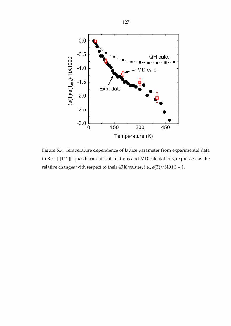
127
-3.0
-2.5
-2.0
-1.5
-1.0
-0.5
0.0
Exp. data
QH calc.
MD calc.(a
(T)/
a(T
40
K)-
1)X
10
00
0 150 300 450
Temperature (K)
Figure 6.7: Temperature dependence of lattice parameter from experimental data
in Ref. [ [111]], quasiharmonic calculations and MD calculations, expressed as the
relative changes with respect to their 40 K values, i.e., a(T)/a(40 K) − 1.
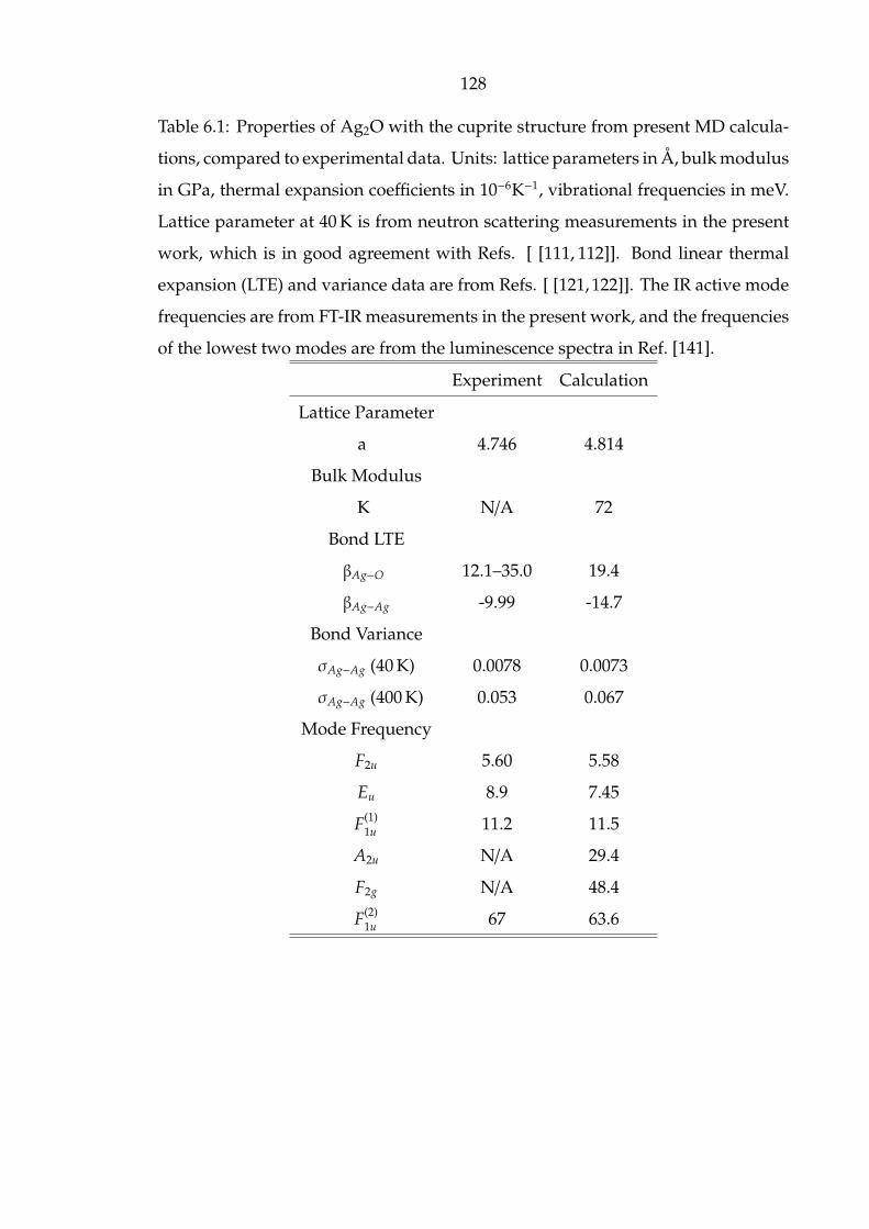
128
Table 6.1: Properties of Ag2O with the cuprite structure from present MD calcula-
tions, compared to experimental data. Units: lattice parameters in Å, bulk modulus
in GPa, thermal expansion coefficients in 10−6K−1, vibrational frequencies in meV.
Lattice parameter at 40 K is from neutron scattering measurements in the present
work, which is in good agreement with Refs. [ [111, 112]]. Bond linear thermal
expansion (LTE) and variance data are from Refs. [ [121,122]]. The IR active mode
frequencies are from FT-IR measurements in the present work, and the frequencies
of the lowest two modes are from the luminescence spectra in Ref. [141].
Experiment Calculation
Lattice Parameter
a 4.746 4.814
Bulk Modulus
K N/A 72
Bond LTE
βAg−O 12.1–35.0 19.4
βAg−Ag -9.99 -14.7
Bond Variance
σAg−Ag (40 K) 0.0078 0.0073
σAg−Ag (400 K) 0.053 0.067
Mode Frequency
F2u 5.60 5.58
Eu 8.9 7.45
F(1)1u 11.2 11.5
A2u N/A 29.4
F2g N/A 48.4
F(2)1u 67 63.6

129
0 10 20 30 40 50 60 70
F1u
(IR)F2g
A2u
F1u
(IR)Eu
F2u
40K+
0.45GPa
400K
200K
40K
Energy (meV)
P(ω
) (a
.u)
(1) (2)
Figure 6.8: Phonon modes simulated by MD and projected on the Γ-point, at
temperatures and pressures as labeled. The normal-mode frequencies calculated
from harmonic lattice dynamics are shown as vertical dashed lines in red. The
group symmetry for each mode is shown at the bottom.

130
0 100 200 300 400
-3.0
-2.5
-2.0
-1.5
-1.0
-0.5
0.0
0.5
F1u
F2g
Temperature (K)
Mo
de
Sh
ihft (m
eV
)
F1u
(1)
(2)
(a)
F1u
F1u
(2)
(1)
(b)
0 100 200 300 400
1
2
4
8
16
F2g
Life
tim
e (
ps)
Temperature (K)
Figure 6.9: (a) Temperature dependent frequency shifts of the Ag-dominated F(1)1u
mode and the O-dominated F2g and F(2)1u modes from FT-IR (black), compared
with the MD simulated peaks (red) such as in Fig. 6.8. (b) The lifetimes of the
corresponding modes at temperatures from 40 to 400 K, from FT-IR (black) and the
MD simulated peaks (red).

131
6.4 Anharmonic Perturbation Theory
6.4.1 Computational Methodology
Cubic anharmonicity gives rise to three-phonon processes, which are an important
mechanism of phonon-phonon interactions. The strengths of the three-phonon
processes depend on two elements – the cubic anharmonicity tensor that gives
the coupling strengths between three phonons, and the kinematical processes de-
scribed by the two-phonon density of states (TDOS). [2, 48, 142]
From Ipatova, et al. [46], an anharmonic tensor element for a process with the
initial phonon mode j at the Γ-point and s phonons is
V( j; q1 j1; ...; qs−1 js−1) =1
2s!
(~
2N
) s2
N∆(q + q1 + · · · + qs−1)
×[ωω1 · · · ωs−1 ]12 C( j; q1 j1; ...; qs−1 js−1) (6.2)
where the phonon modes qi ji have quasiharmonic frequencies ωi and occupan-
cies ni. The C(.)’s are expected to be slowly-varying functions of their argu-
ments. [143] We assume the term C( j; q1 j1; ...; qs−1 js−1) is a constant for the initial
phonon j, and use it as a parameter when fitting to trends from MD or experiment.
Although C( j; q1 j1; q2 j2) changes with j1 and j2, an average over modes,
⟨C(.)⟩ =∑
1,2 C( j; q1 j1; q2 j2)∑1,2 1
(6.3)
is found by fitting to experimental or simulational results, where 1, 2 under the
summation symbol represent qi ji. We define the cubic fitting parameter as
C(3)j = ⟨C( j; q1 j1; q2 j2)⟩ (6.4)
The second key element of perturbation theory is that interacting phonons
satisfy the kinematical conditions of conservation of energy and momentum. This
condition is averaged over all phonons with the two-phonon density of states
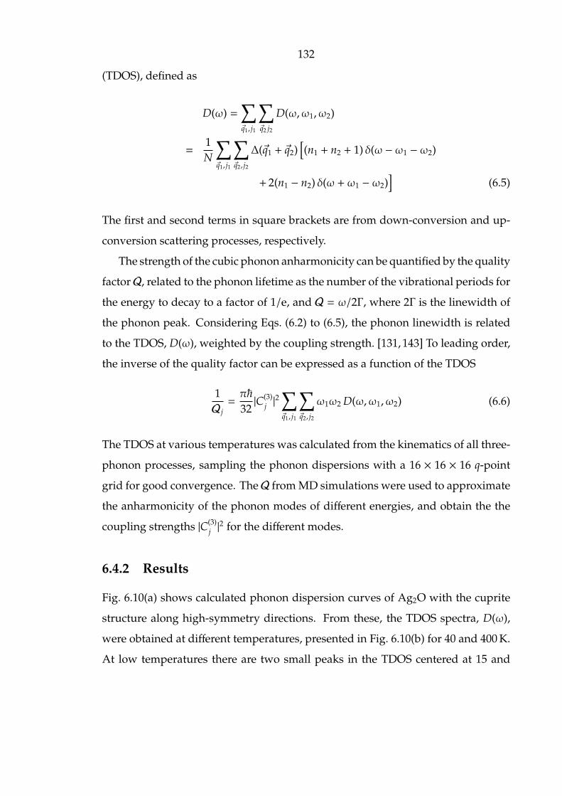
132
(TDOS), defined as
D(ω) =∑q1, j1
∑q2 j2
D(ω,ω1,ω2)
=1N
∑q1, j1
∑q2, j2
∆(q1 + q2)[(n1 + n2 + 1) δ(ω − ω1 − ω2)
+ 2(n1 − n2) δ(ω + ω1 − ω2)]
(6.5)
The first and second terms in square brackets are from down-conversion and up-
conversion scattering processes, respectively.
The strength of the cubic phonon anharmonicity can be quantified by the quality
factorQ, related to the phonon lifetime as the number of the vibrational periods for
the energy to decay to a factor of 1/e, and Q = ω/2Γ, where 2Γ is the linewidth of
the phonon peak. Considering Eqs. (6.2) to (6.5), the phonon linewidth is related
to the TDOS, D(ω), weighted by the coupling strength. [131, 143] To leading order,
the inverse of the quality factor can be expressed as a function of the TDOS
1Q j=π~32|C(3)
j |2∑q1, j1
∑q2, j2
ω1ω2 D(ω,ω1,ω2) (6.6)
The TDOS at various temperatures was calculated from the kinematics of all three-
phonon processes, sampling the phonon dispersions with a 16 × 16 × 16 q-point
grid for good convergence. TheQ from MD simulations were used to approximate
the anharmonicity of the phonon modes of different energies, and obtain the the
coupling strengths |C(3)j |2 for the different modes.
6.4.2 Results
Fig. 6.10(a) shows calculated phonon dispersion curves of Ag2O with the cuprite
structure along high-symmetry directions. From these, the TDOS spectra, D(ω),
were obtained at different temperatures, presented in Fig. 6.10(b) for 40 and 400 K.
At low temperatures there are two small peaks in the TDOS centered at 15 and

133
65 meV. Our calculation showed that the peak at 15 meV is from the decay processes
of one Ag-dominated mode into two with lower frequencies, i.e., Ag 7→ Ag + Ag.
The peak at 65 meV originates from spontaneous decay of one O-dominated mode
into another O-dominated mode of lower frequency and one Ag-dominated mode.
At high temperatures there are more down-conversion processes, but an even
greater change in up-conversion processes. Figure 6.10(b) shows how the strong
down-conversion peaks at low temperatures grow approximately linearly with
temperature, following the thermal population of phonon modes involved in the
interactions. Near the peak at 65 meV, one up-conversion band centered at 50 meV
is also strong. This band comprises scattering channels in which one O-dominated
mode is combined with a Ag-dominated mode to form a higher frequency O-
dominated mode, i.e., O 7→ O − Ag. At the low energy side, there is another
band below 15 meV from two types of up-conversion processes. One is from Ag-
dominated modes alone, i.e., Ag 7→Ag −Ag. The other involves two O-dominated
modes, i.e., Ag 7→ O − O, owing to the increased number of higher energy O-
dominated modes that can participate in these processes at higher temperatures.
Figure 6.11 shows the inverse of quality factors, 1/Q, of the F(1)1u , F2g, F(2)
1u and A2u
phonon modes from FT-IR and MD calculations, together with the best theoretical
fits with Eq. (6.6). These modes are near the centers of main features of the phonon
DOS shown in Fig. 6.2, i.e., the peaks 1, 2, 3 and the gap in between, respectively,
and are useful for understanding the overall anharmonicity. As shown in Fig. 6.11,
at higher temperatures the quality factors decrease substantially. At 400 K, the F(1)1u ,
F2g, F(2)1u modes have low Q values from 12 to 15, but the A2u mode has a much
larger value of 26. With a single parameter |C(3)j |2 for each mode, good fittings to
the quality factors are obtained. The fitting curves and the corresponding values of
the parameters |C(3)j |2 are presented in Fig. 6.11. The |C(3)
j |2 values do not vary much
among different modes, so the typical assumption of a slowly varying C(.) seems
reasonable.

134
(a.u.)
D
(ω)
0
10
20
30
40
50
60
70
RX
Energy (meV)
M
(a)
0 20 40 60 80 100 120
0.0
0.5
1.0
1.5 Ag Ag Ag
Ag Ag+Ag
O O Ag
O O+Ag
Energy (meV)
Ag O O
Г Г
(b)
Figure 6.10: (a) Calculated phonon dispersion along high-symmetry directions of
Ag2O with the cuprite structure. Γ (0, 0, 0), M (0.5, 0.5, 0), X (0.5, 0, 0), R (0.5, 0.5, 0.5).
(b) The TDOS spectra, D(ω), at 40 K (dashed) and 400 K (solid). The down-
conversion and up-conversion contributions are presented separately as black and
green curves, respectively.
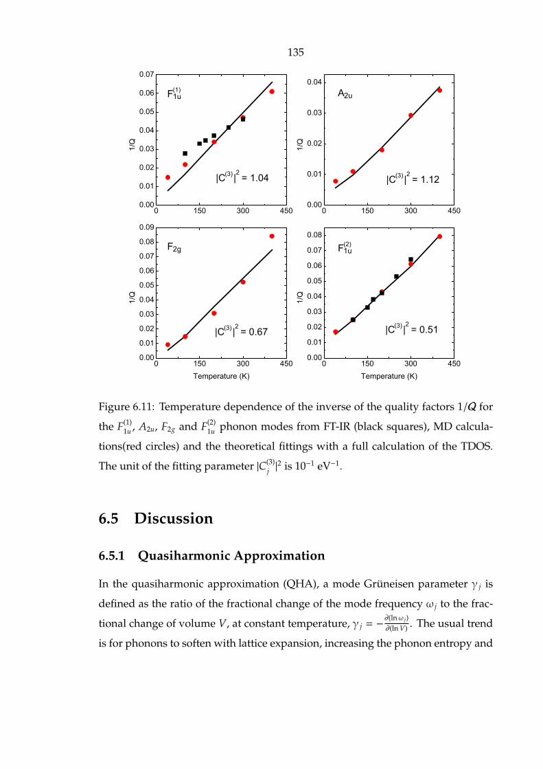
135
0 150 300 4500.00
0.01
0.02
0.03
0.04
0.05
0.06
0.07
0.08
0.09
1/Q
Temperature (K)
0 150 300 4500.00
0.01
0.02
0.03
0.04
1/Q
0 150 300 4500.00
0.01
0.02
0.03
0.04
0.05
0.06
0.07
0.08
1/Q
Temperature (K)
0 150 300 4500.00
0.01
0.02
0.03
0.04
0.05
0.06
0.07
1/Q
F1u(1)
F1u(2)F2g
A2u
|C | = 1.04(3) 2
|C | = 1.12(3) 2
|C | = 0.67(3) 2 |C | = 0.51
(3) 2
Figure 6.11: Temperature dependence of the inverse of the quality factors 1/Q for
the F(1)1u , A2u, F2g and F(2)
1u phonon modes from FT-IR (black squares), MD calcula-
tions(red circles) and the theoretical fittings with a full calculation of the TDOS.
The unit of the fitting parameter |C(3)j |2 is 10−1 eV−1.
6.5 Discussion
6.5.1 Quasiharmonic Approximation
In the quasiharmonic approximation (QHA), a mode Gruneisen parameter γ j is
defined as the ratio of the fractional change of the mode frequency ω j to the frac-
tional change of volume V, at constant temperature, γ j = −∂(lnω j)∂(ln V) . The usual trend
is for phonons to soften with lattice expansion, increasing the phonon entropy and
136
stabilizing the expanded lattice at elevated temperatures. A negative Gruneisen
parameter is therefore expected for the special phonon modes associated with NTE,
such as RUMs. If all the anharmonicity of Ag2O with the cuprite structure is at-
tributed to this volume effect, however, the values of Gruneisen parameters are
approximately –9 for the high energy modes at peaks 2 and 3 of the phonon DOS,
and –20 for the infrared-active F1u mode. These anomalous values may indicate
a problem with the QHA. The QHA method also significantly underestimates the
NTE, and misses the behavior at temperatures above 250 K.
To separate the effects of quasiharmonicity and explicit anharmonicity, the mode
frequency ω j = ω j(V,T) is expressed as a function of volume and temperature
(∂ lnω j
∂T
)P= −γ jβ +
(∂ lnω j
∂T
)V
(6.7)
where j is the phonon mode index, β is the volume thermal expansivity and γ j is
the mode Gruneisen parameter. The left-hand side is the temperature-dependent
frequency shift at constant pressure, and includes contributions from both quasi-
harmonicity and explicit anharmonicity. The first term on the right-hand side, the
isothermal frequency shift as a function of pressure, is the quasiharmonic contri-
bution to the frequency shift. The second term on the right is the pure temperature
contribution to the frequency shift from the explicit anharmonicity. From the dif-
ference of the isobaric and isothermal frequency shifts, the explicit anharmonicity
can be determined.
In a molecular dynamics simulation, the quasiharmonic contribution can be
evaluated explicitly by turning off the temperature-dependent anharmonicity. In
principle, this method is equivalent to the QHA method implemented with self-
consistent lattice dynamics, [119] and in practice we have found this to be true.
For example, we performed simulations at 40 K for volumes characteristic of 400 K,
which produced a pressure of 0.45 GPa. This calculation therefore removed the
temperature effect while preserving the quasiharmonic volume effect at 400 K. The
corresponding phonon DOS curves from MD calculations are shown in Fig. 6.12.
137
By comparing the phonon spectrum of a simulation at 40 K and 0.45 GPa with a
simulation at 400 K, the pure temperature dependence is identified. From the spec-
tra of Fig. 6.12, it is found that the explicit anharmonicity dominates the softening
and broadening of the phonon spectra. All features in the phonon spectra with the
QHA showed little change with temperature, except for small stiffenings at high
energies.
As seen in Fig. 6.12 and in Fig. 6.8, the giant negative Gruneisen parameters are
inconsistent with the results of MD simulations. The volume change alone does
not affect much the phonon lifetimes or frequency shifts. All features in the phonon
spectra generated with the MD-implemented QHA showed little change except for
small stiffening about 0.6 meV at high energies, in agreement with the recent lattice
dynamics QHA calculations. [126]
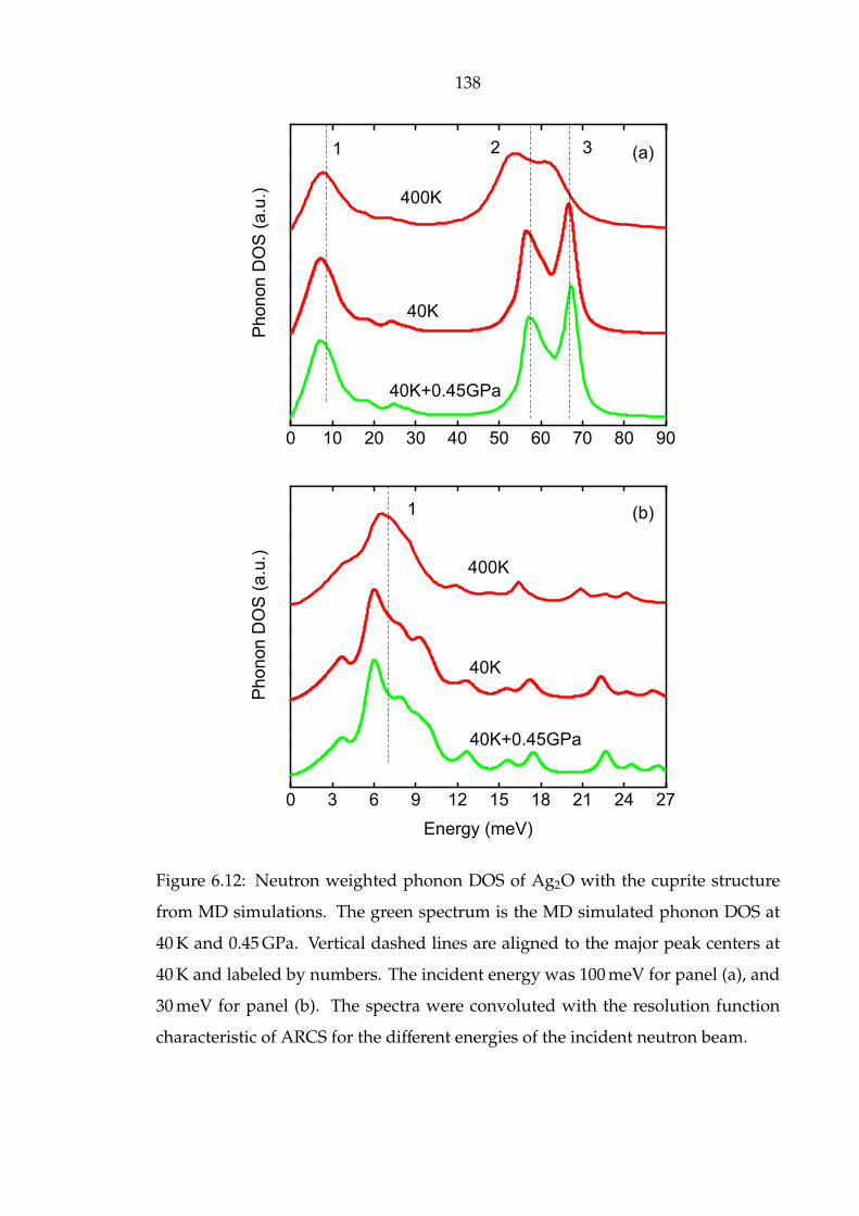
138
0 10 20 30 40 50 60 70 80 90
40K+0.45GPa
400K
Ph
on
on
DO
S (
a.u
.)
40K
0 3 6 9 12 15 18 21 24 27
40K+0.45GPa
400K
Ph
on
on
DO
S (
a.u
.)
Energy (meV)
40K
(a)
(b)
1
1
2 3
Figure 6.12: Neutron weighted phonon DOS of Ag2O with the cuprite structure
from MD simulations. The green spectrum is the MD simulated phonon DOS at
40 K and 0.45 GPa. Vertical dashed lines are aligned to the major peak centers at
40 K and labeled by numbers. The incident energy was 100 meV for panel (a), and
30 meV for panel (b). The spectra were convoluted with the resolution function
characteristic of ARCS for the different energies of the incident neutron beam.
139
6.5.2 Negative Thermal Expansion
Our eigenvector analysis of phonon modes showed that the three low-energy Ag-
dominated F2u, Eu and F1u modes correspond to two distinct types of vibrations.
The F2u mode involves rigid rotations of Ag4O tetrahedra, and could be considered
as RUM. The Eu mode involves the shearing of Ag4O units by changing the Ag-O-
Ag bond angles. The F1u mode measured by infrared spectrometry also shears the
Ag4O units, and includes some displacements of O atoms. Shearing the tetrahedra
was shown to reduce the average vertex-vertex distance [134, 144] and contribute
to the NTE.
In the cuprite structure, the modes associated with the rigid rotations and
the distortions of the Ag4O tetrahedra have similar energies below 10 meV. They
are equally favorable thermodynamically, and both would be active at very low
temperature. As a consequence, there is simultaneously a large deformation of
Ag4O units and a strong contraction of the Ag-Ag shell, as observed experimentally
and computationally at low temperatures. The large thermal distortions of the
Ag4O tetrahedra involve the Ag atoms at the vertices, and their large mass causes
these distortions to occur at low frequencies. Polyhedral units in most other NTE
materials are bridged by the lightweight atoms, such as O and C-N, so the polyhedra
are distorted at significantly higher energies (usually above 40 meV), and may not
distort at lower temperatures.
It is a thermodynamic requirement that the NTE of Fig. 6.7 must go to zero
at T = 0, but the intervening phase transition at 40 K impedes this measurement.
Nevertheless, the steep slope of the lattice parameter with temperature is consis-
tent with the occupancy of phonon modes of 10 meV energy, suggesting that the
QHA model of NTE involves the correct modes, such as the F2u mode (which is a
RUM). These low-energy modes are dominated by motions of the Ag atoms. This
explanation based on the QHA is qualitatively correct, but anharmonic interactions
are large enough to cause the QHA to underestimate the NTE by a factor of two.
140
6.5.3 Explicit Anharmonicity
At temperatures above 250 K, there is a second part of the NTE behavior that is
beyond the predictions of quasiharmonic theory. This NTE above 250 K is predicted
accurately by the ab-initio MD calculations, so it is evidently a consequence of
phonon anharmonicity. The temperature-dependence of this NTE behavior follows
the Planck occupancy factor for phonon modes above 50 meV, corresponding to the
O-dominated band of optical frequencies. In the QHA these modes above 50 meV
do not contribute to the NTE. These modes are highly anharmonic, however, as
shown by their large broadenings and shifts.
For cubic anharmonicity, the two-phonon DOS (TDOS) is the spectral quantity
parameterizing the number of phonon-phonon interaction channels available to
a phonon. For Ag2O with the cuprite structure, the peaks in the TDOS overlap
well with the peaks in the phonon DOS. Most of the phonons therefore have
many possible interactions with other phonons, which contributes to the large
anharmonicity of Ag2O with the cuprite structure, and small Q (short lifetimes).
Although the Q values of most phonon modes in Ag2O with the cuprite structure
are small and similar, the origins of these lifetime broadenings are intrinsically
different. For peak 2 of the phonon DOS, the anharmonicity is largely from the up-
conversion processes: O 7→O−Ag, while for peak 3 it is from the down-conversion
processes: O 7→ O + Ag. The anharmonicity of peak 1 is more complicated. It
involves both up-conversion and down-conversion processes of Ag-dominated
modes. The TDOS also shows why the A2u mode has a larger Q than other modes.
Figure 6.10(b) shows that the A2u mode lies in the trough of the TDOS where there
are only a few phonon decay channels.
Owing to explicit anharmonicity from phonon-phonon interactions, the ther-
modynamic properties of Ag2O with the cuprite structure cannot be understood
as a sum of contributions from independent normal modes. The frequency of an
anharmonic phonon depends on the level of excitation of other modes. At high
temperatures, large vibrational amplitudes increase the anharmonic coupling of

141
modes, and this increases the correlations between the motions of the Ag and O
atoms, as shown by perturbation theory. Couplings in perturbation theory have
phase coherence, so the coupling between Ag- and O-dominated modes at higher
energies, as seen in the peak of the TDOS, causes correlations between the motions
of Ag and O atoms. The ab-initio MD simulations show that anharmonic inter-
actions allow the structure to become more compact with increasing vibrational
amplitude. The mutual motions of the O and Ag atoms cause higher density as
the atoms fill space more effectively. The large difference in atomic radii of Ag and
O may contribute to this effect. Perhaps it also facilitates the irreversible changes
in Ag2O at temperatures above 500 K, but this requires further investigation. For
cuprite Cu2O, which has less of a difference in atomic radii, the thermal expansion
is much less anomalous.
6.6 Conclusions
Phonon densities of states of Ag2O with the cuprite structure at temperatures
from 40 to 400 K were measured by inelastic neutron scattering spectrometry. The
infrared spectra of phonon modes were also obtained at temperatures from 100
to 300 K. Large anharmonicity was found from both the shifts and broadenings of
peaks in the phonon spectra. A normal mode analysis identified the rigid unit
modes and the bending modes of the Ag4O tetrahedra that play key roles in the
negative thermal expansion (NTE) at low temperatures. Some of the NTE can be
understood by quasiharmonic theory, but this approach is semiquantitative, and
limited to temperatures below 250 K.
First principles MD calculations were performed at several temperatures. These
calculations accurately accounted for the NTE and local dynamics of Ag2O with
the cuprite structure, such as the contraction of the Ag-Ag shell and the large
distortion of the Ag4O tetrahedra. The phonon DOS obtained from a Fourier-
transformed velocity autocorrelation method showed large anharmonic effects in
Ag2O, in excellent agreement with the experimental data. A second part of the NTE
142
at temperatures above 250 K is due largely to the anharmonicity of phonon-phonon
interactions and is not predicted with volume dependent quasiharmonicity.
Phonon perturbation theory with the cubic anharmonicity helped explain the
effects of phonon kinematics on phonon anharmonicity of Ag2O with the cuprite
structure. The phonon interaction channels for three-phonon processes are given
by the TDOS, weighted approximately by the phonon coupling strength. The
phonons that are most broadened are those with energies that lie on peaks in the
TDOS. The temperature-dependence of the quality factors Q of individual phonon
modes measured by infrared spectrometry were explained well by anharmonic
perturbation theory. Perturbation theory also showed strong interactions between
the Ag-dominated modes and the O-dominated modes in both up-conversion and
down-conversion processes. In particular, the strong interactions of O-dominated
modes with Ag-dominated modes causes the second stage of NTE at temperatures
above 250 K.
143
Chapter 7
Conclusions
7.1 Summary
Non-harmonic phonon-phonon interaction in solids is a central but poorly under-
stood topic in condensed matter physics. For example, thermodynamic equilib-
rium cannot be achieved with non-interacting harmonic phonons. Finite thermal
conductivity also requires phonon-phonon interactions. We obtained the data of
anharmonic effects in metal oxides (rutile TiO2, cuprite Ag2O, e.g. ) from Raman
spectroscopy, FTIR spectroscopy and inelastic neutron scattering. The focus of
this thesis is more on the models and algorithms we developed, which success-
fully reproduced the vibrational information on anharmonic lattice dynamics. In
particular, we developed the Fourier transformed velocity autocorrelation method
to reproduce the anharmonic phonon energy spectra in solids, and we also used
perturbation theory to investigate microscopically the phonon interaction channels
and interaction intensities in anharmonic processes.
In Chapter 1, fundamental theories of lattice dynamics were reviewed. The
focus was on anharmonic lattice dynamics and phonon-phonon interactions, upon
which most of work presented in this thesis is based. In particular, the Green’s
function method for phonon-phonon interactions was derived in detail, and the
mathematical expressions for anharmonic phonon energy broadening and shift
were proved.
In Chapter 2, the experimental techniques performed in this thesis were dis-
144
cussed. For Raman scattering, the quantum theory and selection rules based on
the group theoretical analysis were discussed in detail. For time-of-flight inelastic
neutron scattering, basic principles of neutron scattering were reviewed, and the
experimental setup and data reduction procedures were introduced.
In Chapter 3, the main computational methods and algorithms that we used
in this study were discussed. This chapter started with a brief review of modern
density functional theory, and molecular dynamics simulations. The focus was on
the methods for phonon calculations, especially the Fourier-transformed velocity
autocorrelation method and the anharmonic phonon-phonon interaction analysis
method.
In Chapter 4, we considered the phonon anharmonicity of rutile TiO2. Raman
spectra of rutile TiO2 were measured at temperatures from 100 K to 1150 K. A dom-
inant role of phonon-phonon kinematics on phonon shifts and broadenings was
reported. Force field MD calculations with the Fourier-transformed velocity auto-
correlation method were also used to perform a quantitative study of anharmonic
effects, successfully accounting for the anomalous phonon anharmonicity of the
B1g mode.
In Chapter 5, we considered the phonon anharmonicity of rutile SnO2. Raman
spectra of rutile SnO2 were measured at temperatures from 83 to 873 K. The pure
anharmonicity from phonon-phonon interactions was found to be large and com-
parable to the quasiharmonicity. The broadening of the B2g mode with temperature
showed an unusual concave downwards curvature. This curvature is caused by
a change with temperature in the number of down-conversion decay channels,
originating with the wide band gap in the phonon dispersions.
In Chapter 6, we considered the phonon anharmonicity of Ag2O with the cuprite
structure. Inelastic neutron scattering measurements on Ag2O were performed at
temperatures from 40 to 400 K, and Fourier transform far-infrared spectra were
measured from 100 to 300 K. The measured phonon densities of states and the in-
frared spectra showed unusually large energy shifts with temperature, and large
linewidth broadenings. First principles molecular dynamics (MD) calculations
145
were performed at various temperatures, successfully accounting for the nega-
tive thermal expansion (NTE) and local dynamics. Using the Fourier-transformed
velocity autocorrelation method, the MD calculations reproduced the large anhar-
monic effects of Ag2O, and were in excellent agreement with the neutron scattering
data. Strong anharmonic effects were found for both phonons and for the NTE.
The lifetime broadenings of Ag2O were explained by anharmonic perturbation
theory, which showed rich interactions between the Ag-dominated modes and the
O-dominated modes in both up- and down-conversion processes.
7.2 Future Work
The study of phonon anharmonicity and phonon-phonon interaction is a difficult
but exciting field. It is difficult because we must consider how phonons interact
with other phonons or with other excitations – an example of a notorious many-
body interaction problem. In comparison, our understanding today about the
vibrational thermodynamics of materials at low temperatures is broad and deep
because it is based on the harmonic model in which phonons are independent,
avoiding issues of anharmonic lattice dynamics.
Phonon anharmonicity is an exciting topic because of its fundamental impor-
tance and broad applications. With the development of modern experimental
techniques and the progress of the anharmonic phonon theories and computa-
tional methodologies, we are in a good position to study the relation between the
phonon anharmonicity and many important thermodynamic properties of materi-
als, for example, thermodynamic phase stability, thermal expansion and thermal
conductivity. Nevertheless, this subject needs new theoretical models and compu-
tational algorithms.
I. Thermodynamic Phase Stability
The ability to predict phase equilibria and structural transformations in solids

146
under pressure and temperature is of great importance to both science and indus-
try. The failure of the harmonic theory mostly arises from the assumption of in-
dependent phonons, which becomes increasingly inaccurate at high temperatures.
For example, although rutile is the most common and stable crystal structure of
TiO2, most of the phonon calculations do not agree well with experimental results.
For example, the anatase phase was calculated to be more stable than the rutile
phase [145]. Moreover, a recent study based on the quasiharmonic approximation
found the low energy modes of rutile to be very soft, and some of them decrease
to zero frequency upon a 0.5% lattice expansion [71]. This suggests an instability
of rutile upon heating. With inelastic neutron scattering data from ARCS, and
very recent first principles MD calculations, we found double well potentials with
a depth of about 2.5 meV for the modes with negative frequencies upon lattice
expansion. This is a classic ”Landau potential”. Using MD simulation at finite
temperatures, the thermal energy of anharmonic modes was found to be consid-
erably larger than the shallow depth of the double wells, ensuring no symmetry
break and structure instability. Moreover, at elevated temperatures, it was found
that these anharmonic modes explore a potential surface that can be approximated
as a quartic form, which accounts for the anomalously large thermal stiffening.
This work is coming along well, and is a good example showing how the phonon
anharmonicity determines the phase stability.
II. Thermal Expansion
Thermal expansion is another anharmonic effect. Recently, negative thermal
expansion (NTE) has been discovered and its potential applications in engineering
are attacting much interest. However, most studies about thermal expansion are
based on harmonic theory or quasiharmonic theory with non-interacting phonons.
In some cases, a harmonic free energy optimization leads to a good estimation of
thermal expansivity, but there are many examples showing that the anharmonic
contribution is significant. The NTE of Ag2O presented in this thesis, for example,

147
is an interesting one [146]. At high temperatures, large vibrational amplitudes
increase the anharmonic coupling of modes, and this tends to increase the correla-
tions between the motions of the Ag and O atoms. The ab-initio MD simulations
show that anharmonic interactions allow the structure to become more compact
with increasing vibrational amplitude. Although we can understand this effect at
a qualitative level, a quantitative model is desirable to describe this interaction.
Because couplings in perturbation theory have phase coherence, the coupling be-
tween Ag- and O-dominated modes at higher energies, as seen in the peak of the
TDOS, is expected to cause correlations between the motions of Ag and O atoms,
and the study of this correlation could be an interesting direction.
III. Thermal Conductivity
In many cases, harmonic lattice dynamics can still be regarded as the leading
order approximation, but such a model predicts an infinite phonon thermal con-
ductivity for a perfect crystal. To obtain a finite thermal conductivity, three-phonon
and higher anharmonic processes must be considered. Thermal conductivity can
be predicted with the Green-Kubo method by using the heat current generated by
MD and taking the autocorrelation [41,42]. The calculation is a little more complex
than the velocity autocorrelation method, but the computational logic and struc-
ture are exactly the same. Our code should be easily extended to this calculation,
which converges fast and is quite robust and accurate.
The Callaway method is also popular [147]. It computes the phonon lifetime
directly, but it also requires the phonon group velocity and energy/momentum
conservation to be calculated explicitly. Actually, several important components
of this method were already developed in the work presented in this thesis. This
method has its own benefit because it can investigate thermal conduction in a mi-
croscopic manner, i.e., contributions from different modes can be clearly identified.
The result from this method can also compare directly with the anharmonic data
obtained in real experiments. For example, using inelastic neutron scattering, we
148
can directly obtain phonon dispersions with lifetime broadening. In our recent
neutron experiment, we got such phonon data on a single crystal of silicon (Si).
These new data could be an important testbed to develop and implement this
method.
IV. Other Theoretical Methods
With the MD calculations and the velocity autocorrelation analysis being well
developed, we can incorporate the MD method with the self-consistent lattice
dynamics model described in Chapter 1. These methods are promising in the
study of anharmonic thermal stabiliy, for example. The benefit of a self-consistent
lattice dynamics calculation is that it is based on a lattice dynamics model, and
therefore once the parameters in this model are known, it could be more efficient
and simpler to get the anharmonic phonon dispersions with very high signal to
noise ratio. It is also interesting to compare the self-consistent lattice dynamics
model with pure MD results because using a mean field harmonic model could be
questionable under very anharmonic conditions.
Another interesting approach might be a frozen ”phonon-phonon interaction”
method. It is based on the direct frozen phonon method, but we can add one more
loop above it. This additional loop would sample different atomic displacements
of different frozen phonons and assign with them appropriate amplitudes. In this
way, we can still take advantage of the well-established frozen phonon method,
but we may also generate an ensemble to simulate the phonon-phonon interactions
and their high-dimensional potential surface. The key to this method is that instead
of assigning displacements randomly, we should build the ensemble according to
the phonon eigenvectors and the target temperature. A MD calculation essentially
provides a dynamic phonon-phonon interactions atmosphere, while in this method,
we are interested in how to freeze these interactions in a controllable manner, and
to extract the potential surface.
Last but not least, the evaluation of anharmonic entropy is quite an interesting

149
and challenging topic. As we presented before, up to now the vibrational entropy
is exclusively based on the harmonic or quasiharmonic approximation, the validity
is under question for a strong anharmonic case. This approximation should fail for
a highly anharmonic material. Although it is more theoretical, the understanding
of the anharmonic vibrational entropy is crucial for advancing the basic theory
of lattice dynamics. In this case, approachs with the harmonic partition function
may be unreliable, and one possible way is to start from the orignial definition
of entropy, i.e., we can sample the phase space from a MD simulation, and try to
obtain the phase volume from those trajectories. Such an approach may include
problems of chaotic dynamics, but rich contributions could come from this.
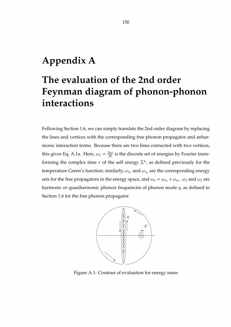
150
Appendix A
The evaluation of the 2nd orderFeynman diagram of phonon-phononinteractions
Following Section 1.6, we can simply translate the 2nd order diagram by replacing
the lines and vertices with the corresponding free phonon propagator and anhar-
monic interaction terms. Because there are two lines connected with two vertices,
this gives Eq. A.1a. Here, ωn =2nπβ~ is the discrete set of energies by Fourier trans-
forming the complex time τ of the self energy Σ⋆, as defined previously for the
temperature Green’s function; similarly, ωn1 and ωn2 are the corresponding energy
sets for the free propagators in the energy space, and ωn = ωn1 +ωn2 . ω1 and ω2 are
harmonic or quasiharmonic phonon frequencies of phonon mode q, as defined in
Section 1.6 for the free phonon propagator.
C
C’
Figure A.1: Coutour of evaluation for energy sums
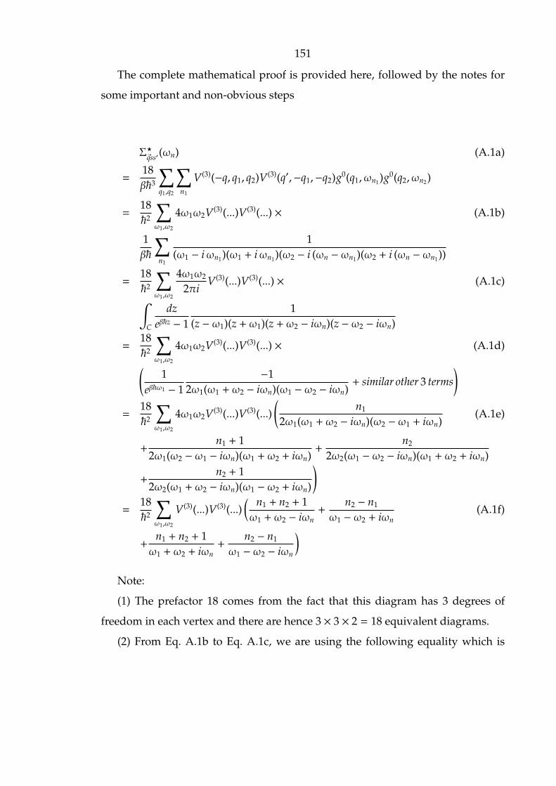
151
The complete mathematical proof is provided here, followed by the notes for
some important and non-obvious steps
Σ⋆qss′(ωn) (A.1a)
=18β~3
∑q1,q2
∑n1
V(3)(−q, q1, q2)V(3)(q′,−q1,−q2)g0(q1,ωn1)g0(q2,ωn2)
=18~2
∑ω1,ω2
4ω1ω2V(3)(...)V(3)(...) × (A.1b)
1β~
∑n1
1(ω1 − iωn1)(ω1 + iωn1)(ω2 − i (ωn − ωn1)(ω2 + i (ωn − ωn1))
=18~2
∑ω1,ω2
4ω1ω2
2πiV(3)(...)V(3)(...) × (A.1c)∫
C
dzeβ~z − 1
1(z − ω1)(z + ω1)(z + ω2 − iωn)(z − ω2 − iωn)
=18~2
∑ω1,ω2
4ω1ω2V(3)(...)V(3)(...) × (A.1d)(1
eβ~ω1 − 1−1
2ω1(ω1 + ω2 − iωn)(ω1 − ω2 − iωn)+ similar other 3 terms
)=
18~2
∑ω1,ω2
4ω1ω2V(3)(...)V(3)(...)(
n1
2ω1(ω1 + ω2 − iωn)(ω2 − ω1 + iωn)(A.1e)
+n1 + 1
2ω1(ω2 − ω1 − iωn)(ω1 + ω2 + iωn)+
n2
2ω2(ω1 − ω2 − iωn)(ω1 + ω2 + iωn)
+n2 + 1
2ω2(ω1 + ω2 − iωn)(ω1 − ω2 + iωn)
)=
18~2
∑ω1,ω2
V(3)(...)V(3)(...)( n1 + n2 + 1ω1 + ω2 − iωn
+n2 − n1
ω1 − ω2 + iωn(A.1f)
+n1 + n2 + 1ω1 + ω2 + iωn
+n2 − n1
ω1 − ω2 − iωn
)Note:
(1) The prefactor 18 comes from the fact that this diagram has 3 degrees of
freedom in each vertex and there are hence 3 × 3 × 2 = 18 equivalent diagrams.
(2) From Eq. A.1b to Eq. A.1c, we are using the following equality which is
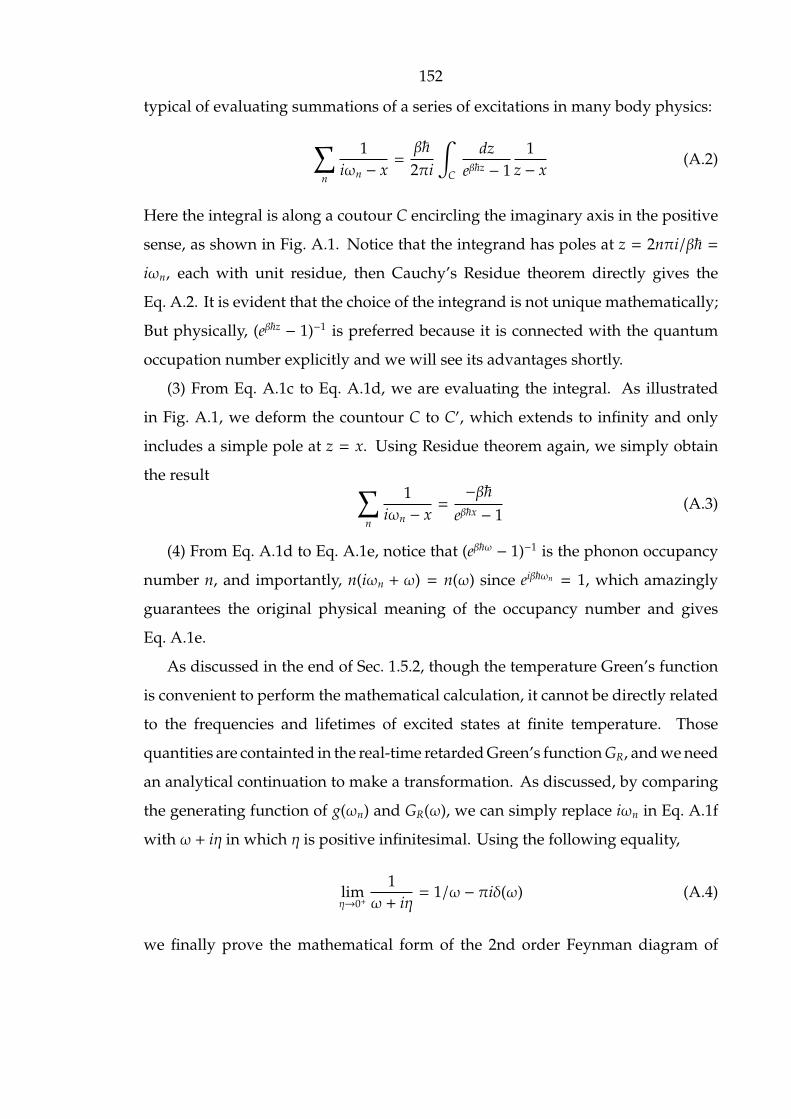
152
typical of evaluating summations of a series of excitations in many body physics:
∑n
1iωn − x
=β~
2πi
∫C
dzeβ~z − 1
1z − x
(A.2)
Here the integral is along a coutour C encircling the imaginary axis in the positive
sense, as shown in Fig. A.1. Notice that the integrand has poles at z = 2nπi/β~ =
iωn, each with unit residue, then Cauchy’s Residue theorem directly gives the
Eq. A.2. It is evident that the choice of the integrand is not unique mathematically;
But physically, (eβ~z − 1)−1 is preferred because it is connected with the quantum
occupation number explicitly and we will see its advantages shortly.
(3) From Eq. A.1c to Eq. A.1d, we are evaluating the integral. As illustrated
in Fig. A.1, we deform the countour C to C′, which extends to infinity and only
includes a simple pole at z = x. Using Residue theorem again, we simply obtain
the result ∑n
1iωn − x
=−β~
eβ~x − 1(A.3)
(4) From Eq. A.1d to Eq. A.1e, notice that (eβ~ω − 1)−1 is the phonon occupancy
number n, and importantly, n(iωn + ω) = n(ω) since eiβ~ωn = 1, which amazingly
guarantees the original physical meaning of the occupancy number and gives
Eq. A.1e.
As discussed in the end of Sec. 1.5.2, though the temperature Green’s function
is convenient to perform the mathematical calculation, it cannot be directly related
to the frequencies and lifetimes of excited states at finite temperature. Those
quantities are containted in the real-time retarded Green’s function GR, and we need
an analytical continuation to make a transformation. As discussed, by comparing
the generating function of g(ωn) and GR(ω), we can simply replace iωn in Eq. A.1f
with ω + iη in which η is positive infinitesimal. Using the following equality,
limη→0+
1ω + iη
= 1/ω − πiδ(ω) (A.4)
we finally prove the mathematical form of the 2nd order Feynman diagram of
153
phonon-phonon interactions as presented in Eq. 4.4(a) and (d), which correspond
to the energy shift and broadening respectively. We can use the same mathematical
manipulation to calculate other diagrams. In particular, that the other two lowest
order diagrams in Fig. 1.2 have no phonon lifetime broadening is because these
terms turn out to have no ωn dependence by the end and hence no imaginary part
when doing the analytical continuation.
154
Appendix B
The Corrrelation method: an examplefor Ag2O with curprite structure
Essentially, we are using the character table to transform the symmetry group rep-
resentation from its natural atomic coordinate basis to its normal basis. Following
Eq. 2.31 and the theory discussed in Section 2.1.3.3, we will provide an example
showing how to derive the group correlation and the selection rule, and the only
tool we need is a character table of point groups that can be found in most books
about group theory.
As described in Section 2.1.3.3, we need to establish the correlation between
the site group and the factor group by comparing the characters in both groups.
Consider first the four equivalent Ag atoms. The D3d sites accommodate four atoms
and it can be shown that Ag atoms are indeed on sites of D3d symmetry. Similarly,
we can find that the two O atoms are on sites of Td symmetry. Since cuprite
structure belongs to the space group O4h , and for the first order Raman scattering,
the factor group inherites the full symmetry of the space group, we therefore need
to establish the correlation between the site groups D3d, Td and the factor group Oh.
Let’s correlate D3d with Oh first. To do this, we need compare the characters of
the operations common to both groups, and find the representations (or modes in
the language of lattice dynamics) of both groups having the same characters. We
can simply write the partial character table of factor group Oh, including only the
operations common to both D3d and Oh. As shown in Table B.1, the irreducible
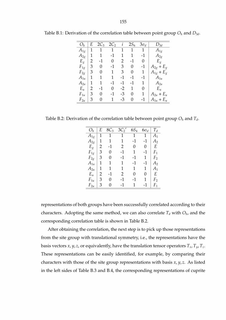
155
Table B.1: Derivation of the correlation table between point group Oh and D3d.
Oh E 2C3 2C2 i 2S6 3σd D3d
A1g 1 1 1 1 1 1 A1g
A2g 1 1 -1 1 1 -1 A2g
Eg 2 -1 0 2 -1 0 Eg
F1g 3 0 -1 3 0 -1 A2g + Eg
F2g 3 0 1 3 0 1 A1g + Eg
A1u 1 1 1 -1 -1 -1 A1u
A2u 1 1 -1 -1 -1 1 A2u
Eu 2 -1 0 -2 1 0 Eu
F1u 3 0 -1 -3 0 1 A2u + Eu
F2u 3 0 1 -3 0 -1 A1u + Eu
Table B.2: Derivation of the correlation table between point group Oh and Td.
Oh E 8C3 3C2′ 6S4 6σd Td
A1g 1 1 1 1 1 A1
A2g 1 1 1 -1 -1 A2
Eg 2 -1 2 0 0 EF1g 3 0 -1 1 -1 F1
F2g 3 0 -1 -1 1 F2
A1u 1 1 1 -1 -1 A2
A2u 1 1 1 1 1 A1
Eu 2 -1 2 0 0 EF1u 3 0 -1 -1 1 F2
F2u 3 0 -1 1 -1 F1
representations of both groups have been successfully correlated according to their
characters. Adopting the same method, we can also correlate Td with Oh, and the
corresponding correlation table is shown in Table B.2.
After obtaining the correlation, the next step is to pick up those representations
from the site group with translational symmetry, i.e., the representations have the
basis vectors x, y, z, or equivalently, have the translation tensor operators Tx,Ty,Tz.
These representations can be easily identified, for example, by comparing their
characters with those of the site group representations with basis x, y, z. As listed
in the left sides of Table B.3 and B.4, the corresponding representations of cuprite

156
Table B.3: Irreducible representation of Ag atoms
Site Group D3d =⇒ Factor Group Dh
irr. reps. trans. type irr. reps. degeneracyA2u 1
A2u Tz F1u 3F1u 3
Eu (Tx, Ty) Eu 2F2u 3
Table B.4: Irreducible representation of O atoms
Site Group Td =⇒ Factor Group Dh
irr. reps. trans. type irr. reps. degeneracyF2 (Tx,Ty,Tz) F1u 3
F2g 3
structures have been identified. Then we can use the correlation tables that we
just built up to map these site group representations to the factor group, which is
straightforward at this point. The only issue here is to adjust the number of each
factor group representations to maintain the degrees of freedom. Take the Ag atom
for example, the degrees of freedom from the site group is simply 4 atoms (per unit
cell) times 3 translational degrees of freedom and is hence equal to 12. On the right
hand side, evidently, the mode degeneracy times the number of corresponding
mode also sum up to 12.
The acoustic modes are also included in this irreducible representation. The
acoustic modes are readily identifiable in factor group because they correspond to
the translational motions of the system. Therefore we can identify them in exactly
the same way as we do for the site group representations with translational sym-
metry. When we consider only those vibrations at the Γ point, the three acoustic
modes are of no physical interest, we can therefore substract them from the irre-
ducible representation. Finally, we obtain the irreducible representation of Ag2O

157
with cuprite structure as follows:
ΓAg2O = ΓAg + ΓO − Γacoust (B.1)
= (A2u + Eu + 2F1u + F2u) + (F1u + F2g) − F1u (B.2)
= A2u + Eu + 2F1u + F2u + F2g (B.3)
At this point, we just need to apply the Selection Rule 2: A mode s is Ra-
man active only if the normal coordinate Qs transforms in the same way as one
of the polarizability tensor components αµν, or equivalently, in the same way as
x2, y2, z2, xy, yz or zx. This is easy to accomplish by checking the corresponding
characters (the same method as being used for identifying the translational sym-
metry described above). Actually in some professional handbooks [9, 10], this
information is explicitly provided along the character table. We find only mode
F2g, a triply degenerate mode, contains the polarizability tensor component and
thereofore is Raman active. Similarly, we find mode F1u is infrared active because
it transforms in the same way as Tx,Ty,Tz. The corresponding eigenvectors can
be derived by using the group projection operator as discussed in Section 2.1.3.3.
The displacement patterns of the normal modes in this example can be found in
Chapter 6.
158
Appendix C
Raman spectra of two-phase and solidsolution phase of Li0.6FePO4 atelevated temperatures
Over the past decade, phosphate-based olivine materials have attracted great re-
search interest as a new class of cathods for lithium-ion rechargeable batteries. In
particular, with the flat discharge voltage of 3.5 V, a theoretical specific capacity of
169 mAh/g and the environmentally friendly constituents, LiFePO4 has been the
focus of much of this research [148,149]. The electrochemical properties of LiFePO4
are limited by a low intrinsic electronic conductivity, and efforts are being made to
improve this feature [150, 151]. The Raman scattering technique clearly represents
a suitable way to investigate the dynamic properties of this material. Although
it is not the focus of the study presented in this thesis, the data we obtained are
interesting and informative for reference and further study.
In particular, Fig. 1 shows the Raman spectra at elevated temperatures of
Li0.6FePO4. The Raman spectra for the two-phase compound (LiFePO4 + FePO4
with phase boundary) show clear evidences of phase transition from the two-phase
to the solid solution above 230 C. As shown in the figure, the sharp Raman lines
diminished at 230 C, caused by a diffusion transfer of lithium ions across the phase
boundary of LiFePO4 and FePO4. Fig. 2 shows evidences that the transition from
the two-phase to the solid solution phase may involve some slow kinetic processes.
Compared with a short heat time (40 mins, 2 hrs and 40 mins), the spectra at long

159
heating time (5 hrs and 40 mins) shows additional energy broadening and shift
features.
12001000800600400200
23C
200C
230C
260C
290C
320C
400C
12001000800600400200
23C
100C
130C
160C
190C
240C
300C
Wavenumbers (cm )-1 Wavenumbers (cm )-1
Figure C.1: Raman spectra at elevated temperatures of two-phase Li0.6FePO4 (leftpanel) and solid solution phase quenched at 400 C(right panel)
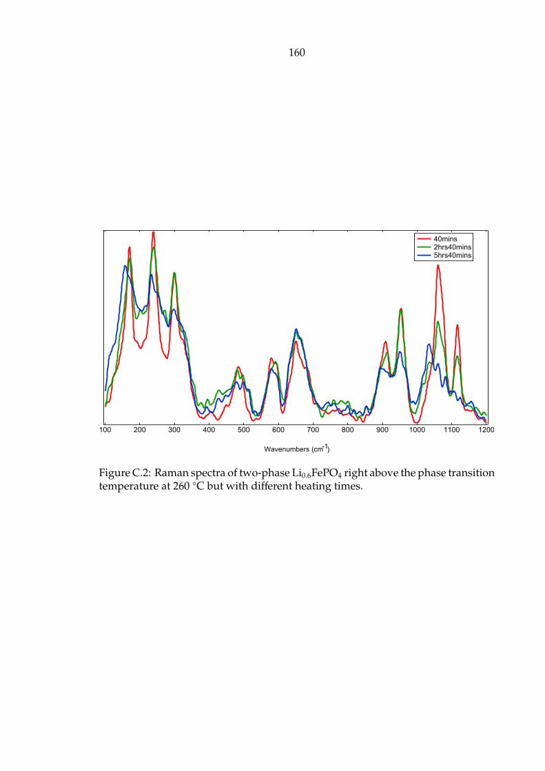
160
120011001000900800700600500400300200100
40mins 2hrs40mins 5hrs40mins
Wavenumbers (cm )-1
Figure C.2: Raman spectra of two-phase Li0.6FePO4 right above the phase transitiontemperature at 260 C but with different heating times.
161
Bibliography
[1] A. L. Fetter and J. D. Walecka. Quantum theory of many particle systems. Dover,
2003.
[2] A. A. Maradudin and A. E. Fein. Phys. Rev., 128:2589, 1962.
[3] J. A. Reissland. The Physics of Phonons. John Wiley and Sons LTD, 1973.
[4] P. Souvatzis, O. Eriksson, M. I. Katsnelon, and S. P. Rudin. Phys. Rev. Lett.,
100:095901, 2008.
[5] O. Hellman, I. A. Abrikosov, and S. I. Simak. Phys. Rev. B, 84:180301, 2011.
[6] R. Loudon. Advances in Physics, 13(52):423, 1964.
[7] A. Compaan and H. Z. Cummins. Phys. Rev. Lett., 31:41, 1973.
[8] P. Y. Yu and Shen. Y. R. Phys. Rev. Lett., 32:373, 1974.
[9] T. Inui, Y. Tanabe, and Y. Onodera. Group theory and its applications in physics.
Springer, 1996.
[10] W. G. Fately, R. R. Dollish, N. T. McDevitt, and F. F. Bentley. Infrared and Raman
Selection Rules for Molecular and Lattice Vibrations. John Wiley and Sons, 1972.
[11] P. Bruesch. Phonons: Theory and Experiments. Springer-Verlag, 1982.
[12] W. L. Chen. Phonon Anharmonicity of Ionic Compounds and Metals. PhD thesis,
California Institute of Technology, 2012.
162
[13] D. L. Abernathy, M. B. Stone, M. J. Loguillo, M. S. Lucas, O. Delaire, X. Tang,
J. Y. Y. Lin, and B. Fultz. Rev. Sci. Instum., 83(1):015114, 2012.
[14] M. G. Kresch. Temperature Dependence of Phonons in Elemental Cubic Metals
Studied by Inelastic Scattering of Neutrons and X-Rays. PhD thesis, California
Institute of Technology, 2009.
[15] B. Fultz, T. Kelley, J. Lin, J. Lee, O Delaire, M. Kresch, M. McKerns, and
M. Aivazis. Experimental inelastic neutron scattering: Introduction to DANSE,
http://docs.danse.us. 2009.
[16] P. Hohenberg and W Kohn. Phys. Rev., 136:864, 1964.
[17] W. Kohn and L. J. Sham. Phys. Rev., 140:1133, 1965.
[18] R. M. Martin. Electronic Structure: Basic Theory and Practical Methods. Cam-
bridge University Press, 2008.
[19] D. M. Ceperley and B. J. Alder. Phys. Rev. Lett, 45:566, 1980.
[20] J. P. Perdew and A. Zunger. Phys. Rev. B, 23:5048, 1981.
[21] J. P. Perdew and Y. Wang. Phys. Rev. B, 45:13244, 1992.
[22] J. P. Perdew, K. Burke, and M. Ernzerhof. Phys. Rev. Lett., 77:3865, 1996.
[23] J. C. Slater. Phys. Rev., 51:846, 1937.
[24] F. Herman. Rev. Mod. Phys., 30:102, 1958.
[25] D. R. Hamann, M. Schluter, and C. Chiang. Phys. Rev. Lett., 43:1494, 1979.
[26] D. Vanderbilt. Phys. Rev. B, 41:7892, 1990.
[27] P. E. Blochl. Phys. Rev. B, 50:17953, 1994.
[28] G. Kresse and D. Joubert. Phys. Rev. B, 59:1758, 1999.
163
[29] D. Marx and J. J. Hutter. Ab Initio Molecular Dynamics: Basic Theory and
Advanced Methods. Cambridge University Press, 2009.
[30] F. Jensen. Introduction to Computational Chemistry. Wiley, 2007.
[31] M. Griebel. Numerical Simulation in Molecular Dynamics. 2007.
[32] J. A. Morrone and R. Car. Phys. Rev. Lett., 101:017801, 2008.
[33] L. Lin, J. A. Morrone, R. Car, and M. Parrinello. Phys. Rev. Lett., 105:110602,
2010.
[34] R. Car and M. Parrinello. Phys. Rev. Lett., 55:2471, 1985.
[35] L. Verlet. Phys. Rev., 159:98, 1967.
[36] H. C. Anderson. J. Chem. Phys., 72:2384, 1980.
[37] S. Nose. Mol. Phys., 52:255, 1984.
[38] W. G. Hoover. Phys. Rev. A, 31:1695, 1985.
[39] P. Giannozzi, S. Baroni, N. Bonini, M. Calandra, R. Car, C. Cavazzoni,
D. Ceresoli, G. L. Chiarotti, M. Cococcioni, I. Dabo, A. Dal Corso, S. de Giron-
coli, S. Fabris, G. Fratesi, R. Gebauer, U. Gerstmann, C. Gougoussis, A. Kokalj,
M. Lazzeri, L. Martin-Samos, N. Marzari, F. Mauri, R. Mazzarello, S. Paolini,
A. Pasquarello, L. Paulatto, C. Sbraccia, S. Scandolo, G. Sclauzero, A. P. Seit-
sonen, A. Smogunov, P. Umari, and R. M. Wentzcovitch. J. Phys.: Condens.
Matter., 21:395502, 2009.
[40] S. Baroni, S. de Gironcoli, A. Dal Corso, and P. Giannozzi. Rev. Mod. Phys.,
73:515–562, Jul 2001.
[41] M. S. Green. J. Chem. Phys., 22:398, 1954.
[42] R. Kubo. J. Phys. Soc. Jpn., 12:570, 1957.

164
[43] D. W. Noid, M. L. Koszykowski, and R. A. Marcus. J. Chem. Phys., 67:404,
1977.
[44] S-T Lin, M. Blanco, and W. A. Goddard. J. Chem. Phys., 119:11792, 2003.
[45] N. de Koker. Phys. Rev. Lett., 103:125902, 2009.
[46] I. P. Ipatova, A. A. Maradudin, and R. F. Wallis. Phys. Rev., 155:882–895, 1967.
[47] X. Tang, C. W. Li, and B. Fultz. Phys. Rev. B, 82:184301, Nov 2010.
[48] X. Tang and B. Fultz. Phys. Rev. B, 84:054303, Aug 2011.
[49] A. L. Linsebigler, G. Lu, and J. T. Yates. catalyst review. Chem. Rev., 95:735,
1995.
[50] U. G. Akpan and B. H. Hameed. Appl. Catal. A-Gen., 375:1, 2010.
[51] Y. Du, N. A. Deskins, Z. Zhang, Z. Dohnalek, M. Dupuis, and I. Lyubinetsky.
Phys. Rev. Lett., 102:096102, Mar 2009.
[52] B. O’Regan and M. Gratzel. Nature(London), 353:737, 1991.
[53] U. Diebold. Surf. Sci. Rep., 48:53, 2003.
[54] P. Balaya. Energy Environ. Sci., 1(6):645–654, 2008.
[55] M. K. Nowotny, L. R. Sheppard, T. Bak, and J. Nowotny. J. Phys. Chem. C,
112:5275, 2008.
[56] D. G. Isaak, J. D. Carnes, O. L. Anderson, H. Cynn, and E. Hake. Phys. Chem.
Minerals, 26:31, 1998.
[57] P. S. Narayanan. Proc. Indian Acad. Sci. Sect. A, 32:279, 1950.
[58] S. P. S. Porto, P. A. Fleury, and T. C. Damen. Phys. Rev., 154(2):522, 1967.
[59] G. A. Samara and P. S. Peercy. Phys. Rev. B, 7(3):1131–1148, 1973.
165
[60] U. Balachandran and N. G. Eror. J. Solid State Chem., 42:276, 1982.
[61] L. G. Liu and T. P. Mernagh. Eur. J. Mineral., 4:45, 1992.
[62] H. Chang and P. Huang. J. Raman Spectrosc., 29:97, 1998.
[63] W. Zhang, Y. He, M. Zhang, Z. Yin, and Q. Chen. J. Phys. D: Appl. Phys.,
33:912, 2000.
[64] X. Feng, Y. Guo, J. Chen, and J. Zhang. J. Biomater. Sci.-Polym. Ed., 18:1443,
2007.
[65] P. S. Peercy and B. Morosin. Phys. Rev. B, 7(6):2779, 1972.
[66] J. Pascual, J. Camassel, P. Merle, B. Gil, and H. Mathieu. Phys. Rev. B, 24:2101–
2108, Aug 1981.
[67] A. Perakis, E. Sarantopoulou, Y. S. Raptis, and C. Raptis. Phys. Rev. B,
59(2):775–782, 1999.
[68] D. J. Lockwood, R. S. Katiyar, and V. C. Y. So. Phys. Rev. B, 28:1983–1987, Aug
1983.
[69] P. S. Peercy. Phys. Rev. B, 8:6018–6020, Dec 1973.
[70] B. Montanari and N. M. Harrison. J. Phys.: Condens. Matter, 16:273, 2004.
[71] P. D. Mitev, K. Hermansson, B. Montanari, and K. Refson. Phys. Rev. B,
81:134303, 2010.
[72] J. A. Thomas, J. E. Turney, R. M. Iutzi, C. H. Amon, and A. J. H. McGaughey.
Phys. Rev. B, 81:081411, 2010.
[73] G. Kopidakis, C. Z. Wang, C. M. Soukoulis, and K. M. Ho. J. Phys.: Condens.
Matter, 9:7071, 1997.
[74] C. W. Li, M. M. McKerns, and B. Fultz. Phys. Rev. B, 80:054304, 2009.

166
[75] J. D. Gale and A. L. Rohl. Mol. Simul., 29:291, 2003.
[76] M. Matsui and M. Akaogi. Mol. Simul., 6:239, 1991.
[77] V. Swamy and J. D. Gale. Phys. Rev. B, 62:5406–5412, Sep 2000.
[78] G. C. Mather, M. S. Islam, and F. M. Figueiredo. Adv. Func. Mater., 17:905,
2007.
[79] M. Mostoller and J. C. Wang. Phys. Rev. B, 32:6773–6786, Nov 1985.
[80] C. Z. Wang, C. T. Chan, and K. M. Ho. Phys. Rev. B, 42:11276–11283, Dec 1990.
[81] J. Menendez and M. Cardona. Phys. Rev. B, 29:2051–2059, Feb 1984.
[82] C. M. B Henderson, K. S Knight, and A. R. Lennie. Open Mineral.J., 3:1, 2009.
[83] J. L. Feldman, L. L. Boyer, P. J. Edwardson, and J. Hardy. Phys. Rev. B,
40:4105–4118, Aug 1989.
[84] E. Liarokapis, E. Anastassakis, and G. A. Kourouklis. Phys. Rev. B,
32(12):8346–8355, 1985.
[85] K. Nishidate and T. Sato. Phys. Rev. B, 46:13773–13778, Dec 1992.
[86] J. Suda and T. Sato. J Phys. Soc. Japan, 66:1707, 1996.
[87] P. G. Klemens. Phys. Rev., 148(2):845, 1966.
[88] M. Balkanski, R. F Wallis, and E. Haro. Phys. Rev. B, 28(4):1928, 1983.
[89] G. D. Barrera, J. A. O. Bruno, T. H. K. Barron, and N. L. Allan. J. Phys.:
Condens. Mattter, 17:217, 2005.
[90] J. A. O. Bruno, N. L. Allan, T. H. K. Barron, and A. D. Turner. Phys. Rev. B,
58:8416–8427, Oct 1998.
[91] R. Mittal, S. L. Chaplot, S. K. Mishra, and Preyoshi P. Bose. Phys. Rev. B,
75:174303, May 2007.

167
[92] P. Merle, J. Pascual, J. Camassel, and H. Mathieu. Phys. Rev. B, 21:1617–1626,
Feb 1980.
[93] B. Fultz. Prog. Mater. Sci., 55:247, 2010.
[94] D. C. Wallace. Thermodynamics of Crystals. Dover Publications, Inc, 1998.
[95] S. J. Smith, R. Stevens, S. Liu, G. Li, A. Navrotsky, J. Boerio-Goates, and B. F.
Woodfield. Am. Miner., 94:236, 2009.
[96] M. Batzill and U. Diebold. Prog. Surf. Sci., 79(2-4):47–154, 2005.
[97] R. S. Katiyar, P. Dawson, M. M. Hargreave, and G. R. Wilkinson. J. Phys. C:
Solid St. Phys., 4:2421, 1971.
[98] H. Hellwig, A. F. Goncharov, E. Gregoryanz, H-K Mao, and R. J. Hemley.
Phys. Rev. B, 67:174110, May 2003.
[99] T. Livneh, Y. Lilach, I. Popov, A. Kolmakov, and M. Moskovits. J. Phys. Chem.
C, 115:17270, 2011.
[100] A. Dieguez, A. Romano-Rodrıguez, A. Vila, and J. R. Morante. J. Appl. Phys.,
90(3):1550–1557, 2001.
[101] F. Gervais and W. Kress. Phys. Rev. B, 31:4809–4814, Apr 1985.
[102] T. Sato and T. Asari. J. Phys. Soc. Japan, 64:1193, 1995.
[103] K. Parlinski and Y. Kawazoe. Eur. Phys. J. B, 13:679, 2000.
[104] H. W. Leite Alves, C. C. Silva, A. T. Lino, P. D. Borges, L. M. R. Scolfaro, and
E. F. da Silva, Jr. Appl. Surf. Sci., 255(3):752–754, 2008.
[105] P. D. Borges, L. M. R. Scolfaro, H. W. Leite Alves, and E. F. da Silva, Jr. Theor.
Chem. Acc., 126:39–44, 2010.
[106] T. Lan, X. Tang, and B. Fultz. Phys. Rev. B, 85:094305, 2012.
168
[107] D. Wang, B. Chen, and J. Zhao. J. Appl.Phys., 101(11):113501, 2007.
[108] J. F. Mammone, M. Nicol, and S. K. Sharma. J. Phys. Chem. Solids, 42:379, 1981.
[109] A. Debernardi. Phys. Rev. B, 57:12847, 1998.
[110] G. Deinzer, G. Birner, and D. Strauch. Phys. Rev. B, 67:144304, 2003.
[111] W. Tiano, M. Dapiaggi, and G Artioli. J. Appl. Crystallogr., 36:1461, 2003.
[112] B. J. Kennedy, Y. Kubota, and K. Kato. Solid State Commun., 136:177, 2005.
[113] S. Bhattacharya and A. Ghosh. Solid State Ionics, 161:61, 2003.
[114] T. Minami. J. Non-Crys. Solids, 56:15, 1983.
[115] W-X Li, C. Stampfl, and M. Scheffler. Phys. Rev. Lett., 90:256102, 2003.
[116] L. Gou and C. Murphy. Nano Lett., 3:231, 2003.
[117] A. K. A. Pryde, K. D. Hammonds, M. T. Dove, V. Heine, J. D. Gale, and M. C.
Warren. J. Phys.-Condens. Matter, 8(50):10973–10982, 1996.
[118] V. Heine, P. R. L. Welche, and M. T. Dove. J. Am. Ceram. Soc., 82:1793, 1999.
[119] C. W. Li, X. Tang, J. A. Munoz, J. B. Keith, S. J. Tracy, D. L. Abernathy, and
B. Fultz. Phys. Rev. Lett., 107(19):195504, NOV 4 2011.
[120] S. a Beccara, G. Dalba, P. Fornasini, R. Grisenti, A. Sanson, and F. Rocca. Phys.
Rev. Lett., 89:025503, Jun 2002.
[121] A. Sanson, F. Rocca, G. Dalba, P. Fornasini, R. Grisenti, M. Dapiaggi, and
G. Artioli. Phys. Rev. B, 73:214305, Jun 2006.
[122] K. W. Chapman and P. J. Chupas. Chem. Mater., 21:425, 2009.
[123] M. Dapiaggi, H. Kim, Emil S. Bozin, S. J. L. Billinge, and G. Artioli. J. Phys.
Chem. Solids, 69:2182, 2008.
169
[124] P. Souvatzis, O. Eriksson, M. I. Katsnelson, and S. P. Rudin. Phys. Rev. Lett.,
100:095901, 2008.
[125] N. Antolin, O. D. Restrepo, and W. Windl. Phys. Rev. B, 86:054119, 2012.
[126] M. K. Gupta, R. Mittal, S. Rols, and S. L. Chaplot. Physica B, 407:2146, 2012.
[127] A. Sanson. Solid State Commun., 151:1452, 2011.
[128] R. Mittal, S. L. Chaplot, S. K. Mishra, and Preyoshi P. Bose. Phys. Rev. B,
75:174303, 2007.
[129] V. Gava, A. L. Martinotto, and C. A. Perottoni. Phys. Rev. Lett., 109:195503,
2012.
[130] A. Putrino and M. Parrinello. Anharmonic raman spectra in high-pressure
ice from Ab Initio simulations. Phys. Rev. Lett., 88:176401, 2002.
[131] T. Lan, X. Tang, and B. Fultz. Phys. Rev. B, 85:094305, 2012.
[132] K. S. Pitzer and W. V. Smith. J. Am. Chem. Soc., 59:2633, 1937.
[133] M. Kresch, M. Lucas, O. Delaire, J. Y. Lin, and B. Fultz. Phys. Rev. B, 77:024301,
2008.
[134] G. I. N. Waterhouse, G. A. Bowmaker, and J. B. Metson. Phys. Chem. Chem.
Phys., 3:3838, 2001.
[135] G. Kresse and J. Furthmuller. Comput. Mater. Sci., 6:15, 1996.
[136] G. Kresse and J. J. Hafner. Phys. Rev. B, 47:558, 1993.
[137] G. Kresse and J. Furthmuller. Phys. Rev. B, 54:11169–11186, 1996.
[138] D. P. Sellan, E. S. Landry, J. E. Turney, A. J. H. McGaughey, and C. H. Amon.
Phys. Rev. B, 81:214305, 2010.
[139] A. Togo, F. Oba, and I. Tanaka. Phys. Rev. B, 78:134106, Oct 2008.
170
[140] P. H. Berens, D. H. J. Mackay, G. M. White, and K. R. Wilson. J. Chem. Phys.,
79:2375, 1983.
[141] F. I. Kreingol’d and B. S. Kulinkin. Soviet Phys.- Semicond., 4:2022, 1970.
[142] Alberto Debernardi, Stefano Baroni, and Elisa Molinari. Phys. Rev. Lett.,
75:1819–1822, 1995.
[143] T. Lan, C. W. Li, and B. Fultz. Phys. Rev. B, 86:134302, 2012.
[144] A. Sanson. Solid State Sciences, 11:1489, 2009.
[145] F. Labat, P. Baranek, C. Domain, C. Minot, and C. Adamo. J. Chem. Phys.,
126:154703, 2007.
[146] T. Lan, C. W. Li, J. L. Niedziela, H. Smith, D. L. Abernathy, G. R. Rossman,
and B. Fultz. Phys. Rev. B, 89:054306, 2014.
[147] J. Callaway. Phys. Rev., 113:1046, 1959.
[148] A. K. Padhi, K. S. Nanjundaswami, and J. B. Goodenough. J. Electrochem.
Soc., 144:1188, 1997.
[149] C. M. Burba and R. Frech. J. Electrochem. Soc, 151:A1032, 2004.
[150] C. Delacourt, C. Wurm, L. Laffont, J. B. Leriche, and C. Masquelier. Solid State
Ionics, 177:333, 2006.
[151] C. Lu, G. T. Fey, and H. Kao. J. Power Sources, 189:155, 2009.