study of the torque vectoring control problem

Alma Mater Studiorum · Università di Bologna

School of Engineering and Architecture · Bologna

Master’s Degree inAdvanced Automotive Electronics Engineering

Class LM-29

STUDY OF THETORQUE VECTORINGCONTROL PROBLEM

Master’s Thesis inApplied Automatic Control

Advisor:Prof. Ing. NICOLA MIMMO

Candidate:GIORGIA FALBO

I Call - I SessionAcademic Year 2018/2019

Contents

List of Symbols 7

1 Introduction 9

1.1 Traction architecture . . . . . . . . . . . . . . . . . . . . . . . . . . . 10

1.2 Torque vectoring . . . . . . . . . . . . . . . . . . . . . . . . . . . . . 11

2 Mathematical Introspection 13

2.1 Euler-Lagrange Equations . . . . . . . . . . . . . . . . . . . . . . . . 13

2.2 Lagrangian Mechanics . . . . . . . . . . . . . . . . . . . . . . . . . . 14

2.3 Moore-Penrose pseudo-inverse . . . . . . . . . . . . . . . . . . . . . . 15

2.3.1 Notation . . . . . . . . . . . . . . . . . . . . . . . . . . . . . . 15

2.4 Equilibrium condition study . . . . . . . . . . . . . . . . . . . . . . . 16

3 Model 19

3.0 Reference Frames . . . . . . . . . . . . . . . . . . . . . . . . . . . . . 19

3.1 Rotation matrices . . . . . . . . . . . . . . . . . . . . . . . . . . . . . 22

3.2 Kinematics . . . . . . . . . . . . . . . . . . . . . . . . . . . . . . . . 26

3.2.1 Justification to the model . . . . . . . . . . . . . . . . . . . . 26

3.2.2 Position Description . . . . . . . . . . . . . . . . . . . . . . . 27

3.2.3 Kinematic Constrains . . . . . . . . . . . . . . . . . . . . . . 29

3.2.4 Car Trim . . . . . . . . . . . . . . . . . . . . . . . . . . . . . 31

3.3 Dynamics . . . . . . . . . . . . . . . . . . . . . . . . . . . . . . . . . 31

3.3.1 Masses Definition . . . . . . . . . . . . . . . . . . . . . . . . . 31

3.3.2 Dynamic Constrains . . . . . . . . . . . . . . . . . . . . . . . 32

3.3.3 Kinetic Energy . . . . . . . . . . . . . . . . . . . . . . . . . . 33

3.3.4 Potential Energy . . . . . . . . . . . . . . . . . . . . . . . . . 34

3.3.5 Work of Non-Conservative Forces . . . . . . . . . . . . . . . . 34

3.3.6 Eulero-Lagrange Equation . . . . . . . . . . . . . . . . . . . . 40

3

CONTENTS

4 Equilibrium Analysis 474.1 Definition of the equilibrium condition . . . . . . . . . . . . . . . . . 474.2 Complete model at the equilibrium conditions . . . . . . . . . . . . . 50

5 Conclusion 59

A Calculations 65A.1 Complete relative rotational matrix . . . . . . . . . . . . . . . . . . . 65A.2 Complete under-vehicle rotational matrix . . . . . . . . . . . . . . . 65A.3 Complete navigation rotational matrix . . . . . . . . . . . . . . . . . 66A.4 Complete i-th wheel reference frame . . . . . . . . . . . . . . . . . . 66A.5 Vehicle position . . . . . . . . . . . . . . . . . . . . . . . . . . . . . . 66A.6 Small angle approximation . . . . . . . . . . . . . . . . . . . . . . . . 67A.7 Simplified position equation . . . . . . . . . . . . . . . . . . . . . . . 67A.8 Partial derivatives used in the position computation . . . . . . . . . 67A.9 Derotation and selection . . . . . . . . . . . . . . . . . . . . . . . . . 68A.10 Derotation and selection computation . . . . . . . . . . . . . . . . . 69A.11 Simplifications . . . . . . . . . . . . . . . . . . . . . . . . . . . . . . 71

B Matlab™Code 73B.1 Variables definition . . . . . . . . . . . . . . . . . . . . . . . . . . . . 73B.2 Matrix definition for position, angles and intertias . . . . . . . . . . . 74B.3 Position first time derivative . . . . . . . . . . . . . . . . . . . . . . . 74B.4 Angular speed definition . . . . . . . . . . . . . . . . . . . . . . . . . 75B.5 Kinetic and potential energy . . . . . . . . . . . . . . . . . . . . . . . 76B.6 Euler-Lagrange equations . . . . . . . . . . . . . . . . . . . . . . . . 76B.7 Symplified Euler-Lagrange equations . . . . . . . . . . . . . . . . . . 78B.8 Additional complete rotational matrices . . . . . . . . . . . . . . . . 79

Bibliography 81

List of Figures 83

List of Tables 85

4

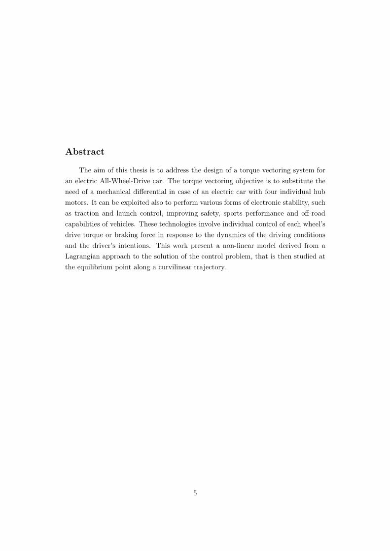
Abstract

The aim of this thesis is to address the design of a torque vectoring system foran electric All-Wheel-Drive car. The torque vectoring objective is to substitute theneed of a mechanical differential in case of an electric car with four individual hubmotors. It can be exploited also to perform various forms of electronic stability, suchas traction and launch control, improving safety, sports performance and off-roadcapabilities of vehicles. These technologies involve individual control of each wheel’sdrive torque or braking force in response to the dynamics of the driving conditionsand the driver’s intentions. This work present a non-linear model derived from aLagrangian approach to the solution of the control problem, that is then studied atthe equilibrium point along a curvilinear trajectory.

5

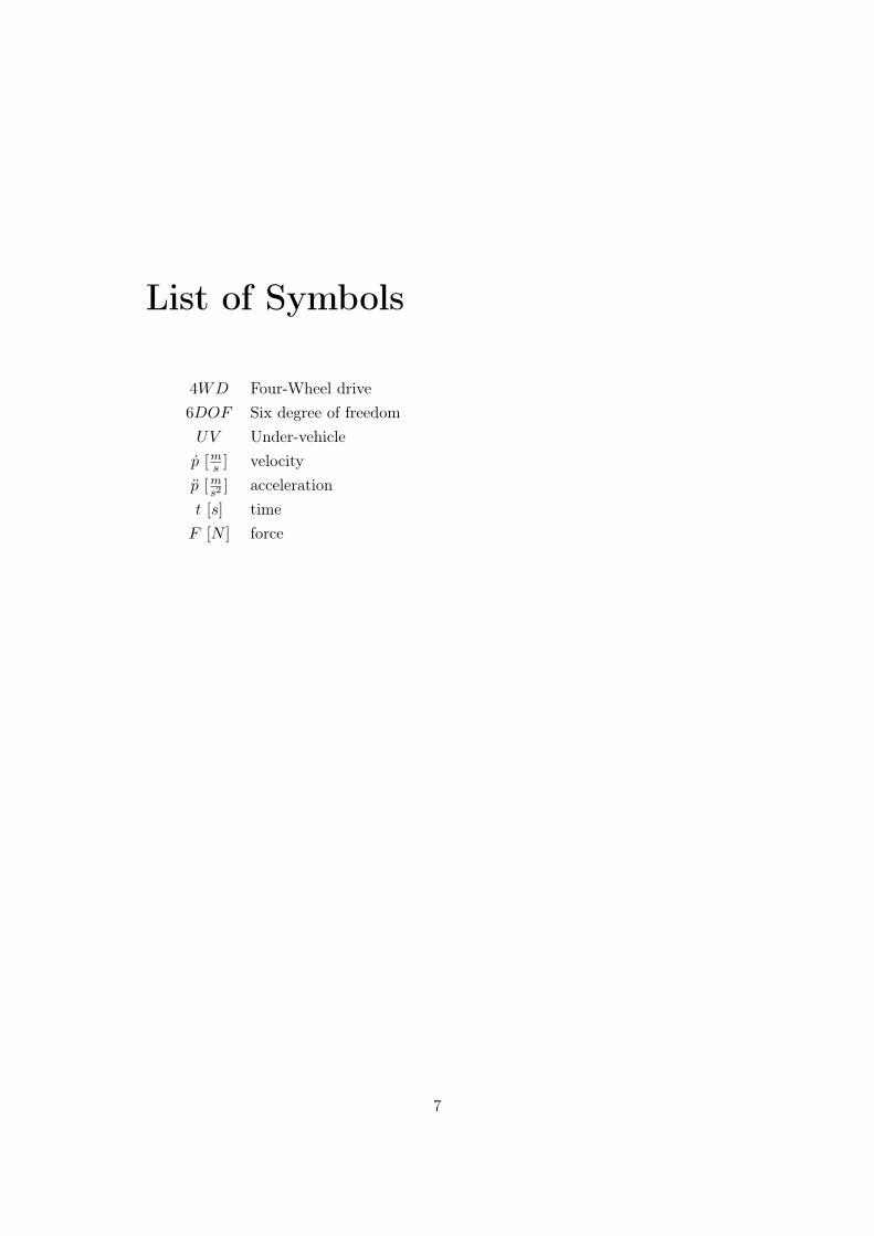
List of Symbols

4WD Four-Wheel drive6DOF Six degree of freedomUV Under-vehiclep [ms ] velocityp [m

s2] acceleration

t [s] timeF [N ] force

7

Chapter 1

Introduction

With the increasing problem of air pollution and global warming, most of thecar manufacturers are starting to develop and sell cars with different topologies ofelectric powertrains. In this context of changes also in the racing world it is possibleto see an increasing effort to make likable also the electric races, as it is possibleto see with FIA Formula E. In this category, the chassy is the same for all carswhile the team has to push above all on the powertrain configuration and the energymanagement.

The energy management in the case of electric vehicles is really important sincenow the benchmark for this new technology is to have the same performances andranges with the internal combustion engine cars, considering a trade off with thecosts. What is important to highlight is that considering the introduction of a newtechnology in the market, there will always be some advantages and disadvantages,but it is really important to let people be aware of the capabilities of the electric

Figure 1.1: Formula E MercedesEQ car for the season 2019/20

9

vehicles.

1.1 Traction architecture

Figure 1.2: Electric All-Wheel drive architecture versus an mechanical all wheel drive

It is possible to make a comparison between the traction architecture of a fourwheel drive internal combustion engine vehicle and a four wheel drive full electricvehicle. In case of a full electric vehicle it is possible to exploit the fact that thepower-train can be designed with four independent electric motors, each one with itsown inverter.

At this point the vehicle control unit can distribute four different torque demandsto the wheels independently, allowing an improvement in performance and stabilityof the vehicle. This chance of having four independently controlled wheels leadsto avoid the need of a mechanical differential, that is normally used with internalcombustion engines vehicle.

A huge advantage of this architecture is the simplification in the transmissionchain, thus leading to the reduction of the total weight of the vehicle and to lessmoving mechanical parts.

Reducing the weight of a mechanical part, it is really important for the vehicleperformance, because instead of having the addition of weight in a fixed point, it can

10

be distribute, through a proper design, to have a better vehicle dynamics.

1.2 Torque vectoring

The torque vectoring, in case of a four wheel drive full electric vehicle, is thetorque distribution on each wheel that can be exploited to have optimal vehicledynamics. The way of how the control is designed depends on the type of vehicleneeds. For instance, for a road car it can be exploited to have a better stability,while in case of a race car, the performance can be stressed as the main goal.

The torque vectoring control can be also designed to allow traction and launchcontrol of the vehicle, acting again on the wheel torque. It depends on how it isdecided to design the control law.

When the vehicle goes around the corner, the weight distribution is not equalon both sides. During the corner the weight get transferred from the inside to theoutside, thus leading to more load on the outside tyres. This is way it is importantto have a different torque on each wheel.

Furthermore, while the vehicle is performing a straight, then during theacceleration, there is a longitudinal weight transfer. The result is that the reartyres experience more load than the rear one, while they are all running at the samespeed. The same happens during the deceleration of breaking, but in the oppositeway.

According to the previous considerations, it is necessary to have on the vehiclea central control unit that calculate, in each instant of time, which is the bettertorque distribution on each wheel according to different measurable parameters. Itis possible to exploit both the power of a feed-forward and feed-back control law.The first one is used to calculate the differentiation of wheel torque during a normaltrajectory, while the second one can be exploited to keep the vehicle on the trajectoryin case of disturbances.

11

Chapter 2

Mathematical Introspection

In this chapter, it will be described the mathematical tools used in the followingmodel solution.

2.1 Euler-Lagrange Equations

Definition: The Euler-Lagrange equations

They are second-order partial differential equation that gives functionalstationary solutions. Where a functional, in mathematical analysis, refers to amapping from a space X into real or complex numbers, with a purpose of having morecomputation like structures. While, a stationary point of a differentiable function ona variable, is a point in which the derivative of the function is zero.

Given the functional:

S(q) =

∫ b

aL(t.q(t), q(t) dt (2.1)

where q is a function of real argument t, then the Euler-Lagrange equation isthe one that has a stationary point given by it.

The Euler-Lagrange equation, then, is given by:

Lx(t.q(t), q(t)− d

dtLv(t.q(t), q(t) = 0 (2.2)

where Lx and Lv denote the partial derivative of L with respect to the secondand third arguments, respectively.

If the dimension of the space X is greater than one, it becomes a system ofdifferential equations, one for each components:

13

∂L

∂qi(t.q(t), q(t)− d

dt

∂L

∂qi(t.q(t), q(t) = 0 for i = 1, ..., n (2.3)

In this specific case, it has been exploited the formulation for several functionsof single variable with single derivative.

In general, if the problem involves finding several functions of a singleindependent variable. Which in the specific case, the function are the motionequation of the vehicle and the single variable is the time t. Then, the formulationof the Euler-Lagrange equations is:

∂L

∂fi− d

dx(∂L

∂f ′i= 0i (2.4)

2.2 Lagrangian Mechanics

The Lagrangian approach, in classical mechanic, can be used to describe theevolution in time of a physical system, since it is equivalent to the solution of Newtonlaw of motion. A huge advantage of this approach is that these equations take thesame form in any system of generalized coordinate systems, thus leading for it to bebetter suited for generalization.

Indeed, in Newton’s laws when it is necessary to include the non-conservativeforces, it is better to express it in Cartesian coordinates. Lagrangian mechanics atthis poi becomes very useful because it allows to bypass any specific coordinatessystem. At this point it is possible to express dissipative and driven forces with thesum of potential and non-potential forces, leading to a set of modified equations. Themain convenience of this approach cam from the fact that the generalized coordiantescan be chosen to suite any requirement, like simplification due to symmetry whichmay help in solve a motion problem.

In general, in order to use this approach, it is necessary to define the Lagrangianas the combination of kinetic and potential energy of the considered system. Thiscan be done in the following way:

L = K − T (2.5)

where K is the potential energy of the system andNow exploiting the definition given in the equation 2.4, it can be found the

equation of motion, which is actually a second-order differential equation, not theactual variable as function of t that can be derived by integrating twice the equation.

This instrument is really powerful since, if the problem involves more than one

14

coordinate, than it would just be necessary to apply the equation 2.4 to each of it.This solution of the problem comes from the principle of stationary action

described in the previous paragraph.

2.3 Moore-Penrose pseudo-inverse

In linear algebra, the pseudo-inverse is a generalization of the inverse of a matrix.It is widely used to find the solution of a system of linear equations which do not

have a unique solution, indeed it peaks the one with the smallest norm. is is uniqueand defined if the entries of the matrix are real or complex and it can be computedusing the singular value decomposition.

2.3.1 Notation

Conventions adopted in the following discussion:

• K denotes one of the fiels of real or complex numbers, R o C. The vector spaceof m× n matrices over K is denoted by Km × n.

• For A ∈ Km×n, A> and A∗ denote the transpose and the conjugate transpose.

• For A ∈ Km × n, im(A) denotes the image of A, the space spanned by thecolumn vectors of A.

• For A ∈ Km × n, ker(A) denotes the kernel of A.

• For any positive integer n, In ∈ Kn × n denotes the Kn × n identity matrix.

Definition: Moore-Penrose pseudo-inverseFor A ∈ Km × n, a pseudo-inverse of A is defined as a matrix A+ ∈ Km × n

that satisfies all the following criteria:

1. AA+A = A

2. A+AA+ = A+

3. (AA+)∗ = AA+

4. (A+A)∗ = A+A

A+ always exist for any matrix A, but when it has full rank (that is defined asthe min{m,n}), it can be expressed with a simple algebraic formula.

At this point it is necessary to distinguish two cases:

15

• n<m The A matrix in this case has linearly independent column, thus leadingto an injective function. This means, it is dealing with an under-sized system:

A+ = (A ∗A)−1A∗ (2.6)

This is called left pseud-inverse.

• n>m The A matrix in this case has linearly independent row, thus leading toa surjective function. This means, it is dealing with an over-sized system:

A+ = A ∗ (A ∗A)−1 (2.7)

This is called right pseud-inverse.

For this specific case, it will be used the right pseudo-inverse.

2.4 Equilibrium condition study

Given a dynamic system, with a finite dimension, continuous in time, non-linearand stationary, that can be described by the state differential equation:

x(t) = f(x(t), u(t) (2.8)

It is possible to consider two different temporal evolution:

1. nominal movement of equilibrium x(t) = x. This can be obtained applying thenominal entry of equilibrium u(t) = u to the system, that is in the nominalinital state x(t = 0) = x⇒ x(t) has to satisfy the following system of equations:

˙x(t) = ˙x = 0 = f(x, u) (2.9)

2. disrupted movement x(t) obtained applying the nominal entry u(t) = u to thesystem in a initial state that is different form the nominal one x0 6≡ x ⇒ x(t)

has to satisfy the following system of equations:{x(t) = f(x(t), u)

x(t0 = 0) = x0(2.10)

The difference between the two movements is the perturbation on the systemstate:

16

δx(t) = x(t)− x ∈ Rn ⇒ x(t) = x+ δx(t) (2.11)

The time evolution of the perturbation is on the state δx(t) is the solution ofthe following differential equation:

δx(t) =d(δx(t))

dt=

=d(x(t)− x

dt=

= x(t)− ˙x =

= f(x(t), u) =

= f(x+ δx(t), u)

(2.12)

that is a non-linear equation in the variable δx(t) and it has the following initialcondition:

δx(t0 = 0) = x(t0 = 0)− x = x0 − x = δx0 6≡ 0 (2.13)

In general the solution of a non linear differential equation δx(t) = f(x +

δx(t), u), δx(t0 = 0) = x0 − x = δx0 is really difficult to find. Furthermore itdepends from both the initial nominal equilibrium state x and from the nominalequilibrium entry u. This means, it depends on the considered equilibrium point.

In case of non-linear and stationary dynamic system, the property of stabilitycan be studied only on a small neighbourhood of a chosen equilibrium state (localstability).

In many cases, with the indirect method of Lyapunov, known also aslinearization method, it is possible to study the local stability at the equilibriumpoint without having to solve the non-linear differential equation.

δx(t) = f(x+ δx(t), u), δx(t0 = 0) = x0 − x = δx0 (2.14)

The function f(x + δx(t), u) can be developed in Taylor series around theequilibrium point.

According to the linearization method, if it is possible to discard all the termsthat contain power of grade greater than one, than the analysis of the stability ofthe equilibrium can be done through the study of the internal stability of an LTIdynamic system.

17

Chapter 3

Model

3.0 Reference Frames

Definition: Rigid bodyIt is a solid body with no deformation and if it as a deformation, it is so small

that it can be neglected. In a rigid body the distance among each point remainsconstant regardless any external force.Definition: Reference frame

In physics, it consist of an abstract coordinate frame and reference points thatdefine uniquely, in term of position and orientation, the behaviour of an object inthe space. Sometimes the reference frame is attached to the modifier.

First of all, it is necessary to define two parts of the car:

1. Body : representation of a rigid body with 6 degree of freedoms (threetraslations and three rotatios), which is attached to the road by means of an

Figure 3.1: Definition of the Body and Under-Vehicle systems

19

equivalent system of suspension and tyres. On this part act the aerodynamicforces iFa and the gravity g.

2. Under-Vehicle: ideal part of the vehicle modeled as a rigid body with 6 degreeof freedoms (three traslations and three rotatios) which is attached to the road,which is plane if the suspention are in rest position and it coincides with thebody. On this part act the wheel forces

∑iFw and momenta

∑uτw).

These two parts are connected each other by means of both kinematic anddynamic constraints, which will be described in the section 3.2.3. It it possible tosee a graphical representation of the definition of these system in figure 3.1.

This is the list of reference frame that has been exploited to describe thebehaviour of the car in this case:

• Inertial: FI(OI , xI , yI , zI) where the origin OI is centered in a plane tangentialto the Earth surface, while the axis xI and yI lay on it with the followingdirections:

– xI : oriented toward North

– yI : oriented toward West

While the zI axis is perpendicular to this plane and points upward.

It is possible to see a graphical representation of this reference frame in fig.3.2.

Figure 3.2: Definition of the Inertial reference frame

• Body: FB(OB, xB, yB, zB) where the origin OB is centered in centre of gravityof the car and the axis are defined in the following way:

20

– xB: oriented along the longitudinal symmetry axis

– zB: points upward and lays on the longitudinal symmetry plane

– yB: complete the reference frame according to the right-hand rule


Figure 3.3: Definition of the Body reference frame

• Under-vehicle: FU (OU , xU , yU , zU ) where the centre coincides with the one ofthe body reference frame, OU ≡ OB. The axis are defined by means of arotation of the body reference frame considering the definition of road-relativeangles that will be given at page 24. If the suspensions are in rest position thetwo reference frames are totally coincident.


• Navigation: FN (ON , xN , yN , zN ) where the centre coincides with the one ofthe body reference frame, ON ≡ OB. The important characteristic of thisreference frame is that the axes xN is aligned with the inertial speed of thevehicle. The yN lies on the under-vehicle and it is perpendicular to xN andthe axis zN completes the reference frame according to the right-hand rule.


• i-th Wheel: FWi(OWi , xWi , yWi , zWi) is a fixed reference frame attached to thewheel. Where the origin OWi is centered in the i-th wheel centre of gravityand the axis are defined in the following way:

21

Figure 3.4: Definition of the Under-vehicle reference frame

Figure 3.5: Definition of the Navigation reference frame

– yWi : aligned with the revolution axis of the wheel towards the left side ofthe vehicle

– zWi : points upward and it is aligned with the axis zU

– xWi : complete the reference frame according to the right-hand rule


3.1 Rotation matrices

When it is necessary to consider two different reference frame, it is also necessaryto define the relationship between them. Given two reference frames F1 and F2 anda vector v1 with the coordinate defined in F1, if it is necessary to represent it in

22

Figure 3.6: Definition of the i-th wheel reference frame

the second reference frame, this can be done by means of a linear transformationobtained through the rotational matrix used to define the projection of v1 on theaxis of F2.

One of the most common way of performing rotation in different reference frameis done using the Euler angles that are defined to describe the orientation of a rigidbody in a fixed or moving coordinate reference frame.

The rotation is the combination of three different rotation performed along theaxis, so it necessary also to define three angles of rotation with the correspondingrotational matrices:

• yaw angle (ψ): represents a rotation around the axes z

v′ = R3(ψ)v1 =

cosψ sinψ 0

− sinψ cosψ 0

0 0 1

v1 (3.1)

• pitch angle (ψ): represents a rotation around the axes y

v′′ = R2(θ)v′ =

cos θ 0 − sin θ

0 1 0

sin θ 0 cos θ

v′ (3.2)

• roll angle (ψ): represents a rotation around the axes x

v2 = R1(φb)v′′ =

1 0 0

0 cosφ sinφ

0 − sinφ cosφ

v′′ (3.3)

23

Figure 3.7: Sequence of rotations used to pass from F1 to F2

The composition of these three rotations results in:

v2 = R1(φ)R2(θ)R3(ψ)v1 = 2R1(φ, θ, ψ)v2 (3.4)

Where 2R1(φ, θ, ψ)v2 represent the total rotation matrix between, as it ispossible to see in fig. 3.11. After these consideration it is possible to define allthe rotational angles and matrices among the different reference frame defined in theparagraph 3.0:

• From Inertial to Body :

BRI(φ, θ, ψ) = R1(φ)R2(θ)R3(ψ) (3.5)

where φ, θ and ψ correspond to the Euler angles of pitch, yaw and roll,respectively;

• From Body to Under-vehicle:

URB(φr, θr, ψr) = R1(φr)R2(θr)R3(ψr) (3.6)

where φr, θr and ψr correspond to the relative Euler angles of pitch, yaw androll, respectively. Indeed they describe the relative position of the under-vehiclesystem with respect to the body part, as it is defined in the paragraph 3.0. Thecomplete expression of this matrix can be found in the appendix A.8.

• From Inertial to Under-vehicle:

URI(φu, θu, ψu) = R1(φu)R2(θu)R3(ψu) (3.7)

where φu, θu and ψu correspond to the Euler angles of pitch, yaw and roll,respectively. For this description it will be necessary actually to use the

24

opposite transformation, so from the Under-vehicle to Inertial reference frame.In order to obtain the proper rotational matrix, it is necessary to perform thetranspose of the matrix previously defined:

IRU (φu, θu, ψu) = URI(φu, θu, ψu)> = R>3 (ψu)R>2 (θu)R>1 (φu) (3.8)

This come from the fact that it can be demonstrated that the rotational matrixare orthonormal, which means R> = R−1. The complete expression of thismatrix can be found in the appendix A.2.

• From the Navigation to the Under-vehicle:

URN (0, γU , βU ) = R2(γU )R3(βU ) (3.9)

where βU indicates the side-slip angle. The parameter is really importantfor this discussion and the definition of it will be explained in the chapter 4.1.While γU is the under-vehicle climb angle. The complete expression of thismatrix can be found in the appendix A.3.

• From i-th wheel to Under-vehicle:

URWi(φWi , 0, δWi) = R1(φWi)R3(δWi) (3.10)

where δWi indicates the angle of the wheel with respect to the rest position,during a straight trajectory, needed to perform a curvilinear trajectory. WhileφWi indicates the i-th wheel roll angle, that is its camber angle. The completeexpression of this matrix can be found in the appendix A.4.

FROM TO SYMBOLS ROTATIONSInertial Body BRI φ, θ, ψ

Body Under-vehicle URB φr, θr, ψrInertial Under-vehicle URI φu, θu, ψu

Navigation Under-vehicle URN γU , βUi-th wheel Under-vehicle URWi φWi , δWi

Table 3.1: Summary of all the required coordinate transformation, rotation matricesand angles

25

3.2 Kinematics

3.2.1 Justification to the model

Considering the definition of the vehicle as the assembly of two parts, givenat page 3.0, it is necessary at this point to highlight the main idea that is behindthe description of this model. Starting from a general idea, it will be given thedescription of all the assumption made for this specific case.Definition: Inverted pendulum

An inverted pendulum is a particular type of pendulum which has its centre ofmass above its pivot point, that is the point that should allow the body to keep anull displacement when a rotation is applied on it.

Figure 3.8: Schematic of a cart inverted pendulum

In this case the system considers more degree of freedom with respect to thenormal inverted pendulum that usually as only one. Indeed there are two masses,one of the body and the other one of the under-vehicle system, that are connectedby the means of a torsional spring. This way of outline the vehicle allows the bodyto have both relative roll and pitch with respect to the under-vehicle.

Together with the rotational degrees of freedom, it is necessary also to describethe relative translations that can occur between the body and the under-vehicleidealization. This is done assuming that the only possible translation can beperformed by means of the suspensions is along the z axis.

The following list is the description of all the considered distances within themodel:

• Lx > 0 is the arm linking the centre of mass of the body to the rotation jointin the lateral direction;

• Lz > 0 is the arm linking the centre of mass of the body to the rotation jointin the vertical direction;

26

Figure 3.9: Schematic of the proposed system

• dz(t) represents the relative vertical movement between the two parts (in theunder-vehicle coordinates).

3.2.2 Position Description

The following equation describes the position of the vehicle in the inertialreference frame. From this equation it is possible to understand also how it is definedthe geometry that centre of gravity of the two parts.

ipb = ipu + iRu(Θu)

u

0

0

dz

+ uRb(φr, θr)b

Lx

0

Lz

(3.11)

Where:

• ipu represents the centre of gravity of the under-vehicle (in the inertialcoordinates)

• ipb represents the centre of gravity of the body (in the inertial coordinates)

• Θu = [φu, θu, ψu] are the roll, pitch and yaw angles of the under-vehicle

• φr, θr are the relative roll and pitch angles

The distances, along the different axis, between the centre of gravity are givenaccording to the definition highlighted in the previous paragraph. At this point it ispossible to see that the relative yaw angle between the body and the under-vehiclesystems has been considered always zero. This means that the two parts can’t rotateone on the other along the z axis.

27

Considering this equation, it is necessary to substitute the rotational matricesaccording to the definition given at paragraph 3.1. The complete expression of thissystem is to complicated to be handle manually, so it can be found, just for thereader to know, in appendix A.5.

Small angle approximation

Let us now consider the angles φr and θr sufficiently small:

• φr ≈ 0

such that

– sinφr ≈ φr

– cosφr ≈ 1

• θr ≈ 0

such that

– sin θr ≈ θr

– cos θr ≈ 1

This approximation comes from the fact that it is possible to assume that allthe relative rotations generated by the suspension systems can be neglected.

It is possible to find the complete result of this approximation in the appendixA.6. Since also this expression is not as easy to be handle, it has been tried to shrinkthe system using the following definitions:

A =

(sinφu sinψu + cosφu cosψu sin θu)

− (cosψu sinφu − cosφu sinψu sin θu)

cosφu cos θu

(3.12)

B =

cosψu cos θu

cos θu sinψu

− sin θu

(3.13)

C =

(cosφu sinψu − cosψu sinφu sin θu)

− (cosφu cosψu + sinφu sinψu sin θu)

− cos θu sinφu

(3.14)

This come from the equation that can be found in the appendix A.7.

28

Thus leading to the far more compact equation:

ipb ≈ ipu +A (dz − Lx θr + Lz) +B (Lx + Lz θr) + C (Lz φr) (3.15)

At this point it is necessary to compute the first derivative of ipb to express thevehicle speed in the inertial reference frame, that is given by:

ipb = ipu + A (dz − Lx θr + Lz) +A(dz − Lx θr

)+

+B (Lx + Lz θr) +Bθr + CL (Lz φr) + Cφr(3.16)

where the following substitutions holds:

•A =

∂A

∂φuφu +

∂A

∂θuθu +

∂A

∂ψuψu (3.17)

•B =

∂B

∂φuφu +

∂B

∂θuθu +

∂B

∂ψuψu (3.18)

•C =

∂C

∂φuφu +

∂C

∂θuθu +

∂C

∂ψuψu (3.19)

The complete expression of these derivatives can be found in the appendix A.8.This equation for the small angles approximation previously described, i.e.

φr, θr ≈ 0, is simplified as follows:


)+


3.2.3 Kinematic Constrains

In this paragraph it will be described which are the kinematic constrains thatlink all the systems used to describe the vehicle behaviour. The links are above allbetween the body and the under-vehicle systems. It is important to highlight thatit has been assumed that a movement of the body, as a consequence in the motionof the under-vehicle and vice-versa. As a consequence, this leads to necessity ofdescribing how the single kinematic of the two system influence actually the overallbehaviour of the vehicle.

This comes from the fact that many reference system are exploited for thedescription of the vehicle behaviour and the complete model need to be coherentwith all the assumption that links all the definitions.

29

1. Under-vehicle reference frame with respect to Inertial reference frameThe under-vehicle plane, (OU , xU , yU ), is coincident with the correspondinginertial, OI , xI , yI). It means that the vehicle is leveled with the North-Westplane and the under-vehicle reference frame is aligned with the inertial one,with except for a rotation around the third axis z of the angle ψu. Thisassumption will be exploited after the computation of the Eulero-Lagrangeequations, since to calculate it it is necessary to consider all the possible degreeof freedom.

• φU = 0

• θU = 0

From the physical point of view, it means that the wheels are always attachedto the ground and the vehicle is not jumping or flying.

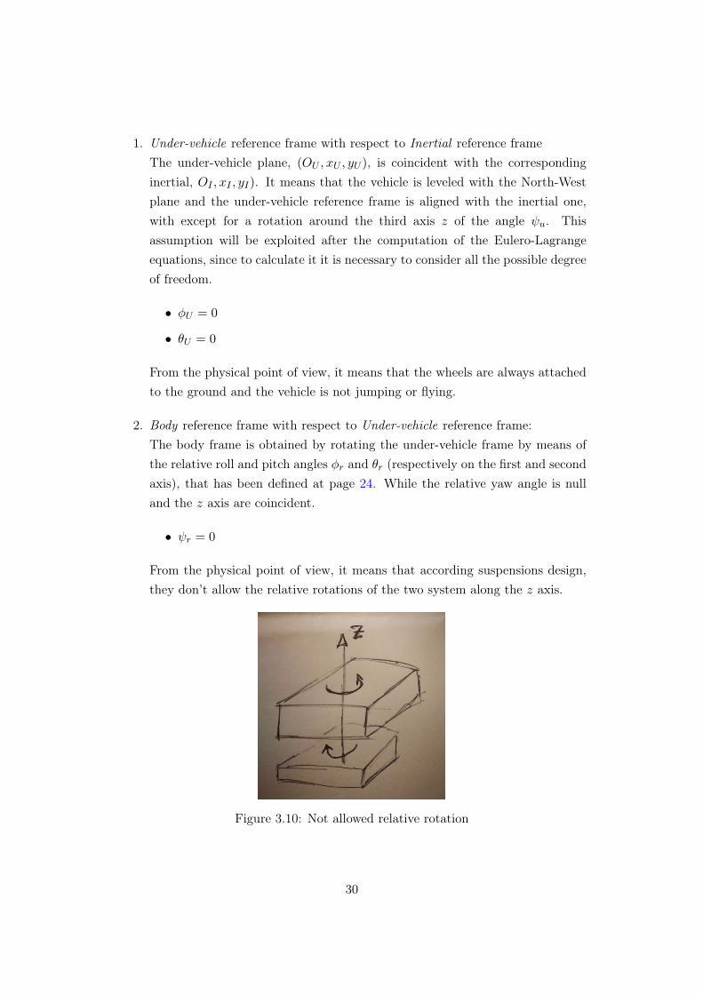
2. Body reference frame with respect to Under-vehicle reference frame:The body frame is obtained by rotating the under-vehicle frame by means ofthe relative roll and pitch angles φr and θr (respectively on the first and secondaxis), that has been defined at page 24. While the relative yaw angle is nulland the z axis are coincident.

• ψr = 0

From the physical point of view, it means that according suspensions design,they don’t allow the relative rotations of the two system along the z axis.

Figure 3.10: Not allowed relative rotation

30

3.2.4 Car Trim

In this paragraph, it will be described which are the further assumption on thevehicle attitude.

• Null camber angle φWi = 0:The camber angle of a wheel is the inclination that is can have along x, so withrespect to the frontal section. In this case, it is considered that the suspensionkinematic chain doesn’t allow the following behaviour, but onth the first case.

Figure 3.11: Camber angle examples

• Null climb angle γU :The climb angle describe the road inclination according the speed of the vehicle.It come as a consequence of the considered type of road, as for example thevehicle climbing a mountain or coming down from a descent. Assuming a nullclimb angle means that in this case the vehicle is moving on a flat road.

3.3 Dynamics

3.3.1 Masses Definition

As the vehicle as been arranged as the sum of two subsystem, the body and theunder-vehicle, it is also important to define which are the masses that belongs twothe two sub-system and where the centre of gravity are located.

The masses of the two sub-systems includes the following vehicle parts:

• Sprung mass (mb): body and chassy

31

• Unsprung mass (mu): wheels, brakes, hubs, axles, A-frames, springs and shockabsorbers

The position of the centre of gravity of the two subsystem considering theposition of the total centre of gravity is important also for the definition used atpage 27.

Figure 3.12: Weight distribution of the vehicle

Through this image, it is possible to understand also where the dynamicconstrains have been applied, from the schematic point of view.

3.3.2 Dynamic Constrains

As it has been highlighted at page 20, some of the external forces are ideallyapplied on the body and others are applied to the under-vehicle. As a consequence,it is really important to describe how the forces applied to one system influence theother. For instance, if the vehicle is accelerating the under-vehicle is going to movefaster, while the body is initially dragged by it.

The dynamical link between the two subsystem is defined by a system of bothtranslational and rotational assembly of springs and dumpers that follows the samerelative degree of freedom left from the kinematic constrains.

The forces and momenta provided by the dumper-spring system are thefollowing:

32

(a) Horizontal system of spring and dumper (b) Vertical system of spring and dumper

• Force along the zU axis:Fz = −kzdz − βzdz (3.21)

• Momentum along the xU axis:

Mx = −kφrφr − βφr φr (3.22)

• Momentum along the yU axis:

My = −kθrθr − βθr θr (3.23)

3.3.3 Kinetic Energy

The kinetic energy associated to the system is:

T =1

2mu

ip>uipu +

1

2mb

ip>bipb +

1

2

[φu θu ψu

] Jxu Jxyu Jxzu

Jxyu Jyu Jyzu

Jxzu Jyzu Jzu

φu

θu

ψu

+

+1

2

[φr θr ψu

] Jxb Jxyb JxzbJxyb Jyb JyzbJxzb Jyzb Jzb

φr

θr

ψu

(3.24)

In this formula, it is necessary to substitute the expression of the body speedipu, with the one found at paragraph 3.2.2 as function of the under-vehicle, in orderto consider the geometry of the system.

The contribution to the kinetic energies come from all the masses and inertiasof the system according to the previous definition of the two sub-system.

33

3.3.4 Potential Energy

From the assumption given at paragraph 3.2.3, it is possible to deduce that theunder-vehicle is always at ground level (zero level). Thus leading to the fact thatthere is not potential energy associated with the mass mu, i.e. ipu(3) ≡ 0). As aconsequence the potential energy depends only on mb and the energy associated tothe spring-dumper systems, according to the following formula:

K =1

2kzd

2z +

1

2kφrφ

2r +

1

2kθrθ

2r +mbg(Lz + dz) (3.25)

3.3.5 Work of Non-Conservative Forces

In this paragraph, it is going to be described the non-conservative forces thatacts on the the vehicle. This is necessary in order to find the work of these forces,that will be used for the equalities in the Eulero-Lagrange equations, at paragraph3.3.6.

Wheel Forces

Figure 3.14: Free body diagram of a driven wheel represented in two dimension

In order to have the generation of forces between the pneumatic and the road,it is necessary to have a relevant slip in the zone where the contact happens. In thiscase it is necessary to have a null relative speed between the two parts. The sliptakes into account the scenario where the deformation of the pneumatic compensatethe difference of speed between the wheel and the road.

For this model the forces between the tyres and the ground on the three axiscan be expressed all as function of FWWiz

. This is possible because the vertical forceis the one that determines the load on the road depending on different coefficients.

The force produced by tires in contact with the ground can be expressed asfollows:

34

FWWi= FWWiz

λLiλTi

µ (λTi) + CR(ViWix

)λSiλTi

µ (λTi)

1

(3.26)

where the total, longitudinal and side slip ratio are defined by means of thefollowing equations:

• λLi longitudinal slip ratio

λLi =ωir − ViWxvmax

(3.27)

• λSi side slip ratio

λSi =−ViWyvmax

(3.28)

• λTi total slip ratioλTi = λ2Li + λ2Si (3.29)

Where the definition of vmax is given by:

vmax =

√(ViWy

)2+ (max {|ViWx − ωir|, |ViWx |, |ωir|}) (3.30)

while the wheel speed expressed in the wheel reference frame, V Wi , depends on

the vehicle speed according to the following rotation:

V Wii =U RWi(0, 0, δWi)V

Ui (3.31)

while the definition of V Ui is:

V Ui = ωUU × rUi + URN (0, 0, βU )V N

OB(3.32)

It is also necessary to show the behavior of the following coefficients throughsome graphs that are obtained with successive experiments, this is due to the factthat is not possible to describe it through a model because they depends on toomany variable:

• µ (λTi) friction coefficient

This graph is actually strictly dependent on the road conditions, as it is possibleto see in figure 3.16. From this graph it is possible to see how for certaincondition the friction coefficient decreases a lot, hence leading to high difficultyin controlling the vehicle.

35

Figure 3.15: Longitudinal friction coefficient at various longitudinal slip

Figure 3.16: Longitudinal friction coefficient for various road conditions

• CR(ViWix

)rolling coefficient

Figure 3.17: Rolling resistance as function of the vehicle speed

36

This parameter takes into account the penetration of the tyre and the road.

In figure 3.18, it is possible to see a schematic of the forces acting on the wheels.

Figure 3.18: Wheel forces

Aerodynamic Forces

The aerodynamic forces in this cases is described in the body reference frameFB, while the speed from which it depends at the beginning is defined in the inertialreference frame FB.

Now the most important parameter to be defined is the air relative speed, thatdescribes the speed of the vehicle taking into account the wind speed, as it show inthe following formula:

V Ia = V I

OB−W I (3.33)

where:

• V IOB

is the inertial vehicle speed, considered as the speed of the centre of gravity;

• W I is the wind speed measured in the inertial reference frame

It is necessary, at this point, to apply a reference transformation since the forceneeds to be described in the body reference frame. This is done in the following way:

V Ba = BRI(φ, θ, ψ)V I

a = BRI(φ, θ, ψ)(V IOB−W I

)(3.34)

37

It is necessary now to define two angles, starting from this velocity, in order toexplain the dependence of the force on it.

The two angles are defined according to the following formulas:

• α is the aerodynamic angle of attack :

α = tan−1

V Bax√(

V Bax

)2+(V Bay

)2 (3.35)

It describes the angle that the air relative speed has with the xb − yb plane ofthe body reference frame

• β is the aerodynamic side slip angle:

β = sin−1

V Bay√(

V Bax

)2+(V Bay

)2 (3.36)

If the air relative speed is projected on the xb − yb plane of the body referenceframe, this is the angle that is present between the projection and the xB axis.

where V Ba is the following column vector:

V Ba =

V Bax

V Bay

V Bay

(3.37)

At this point it is possible to describe the relationship that link the aerodynamicforces, FBa expressed in the body reference frame FB.

The forces are function of the impact pressure, that is computed in the followingway:

P =1

2ρV 2

a (3.38)

This parameter has to be multiplied by the reference surface of the vehicle Sand the non-dimensional coefficients CX , CY and CZ .

The formula describing this behaviour is:

FBa =1

2ρV 2

a

CX

CY

CZ

(3.39)

38

where:

• Va = ||V Ba || = ||V I

a || is the modulus of the air relative speed;

• ρ is the density of the air;

• S is the cross section of the vehicle on the plane defined in the body referenceframe by OB, yB and zB.

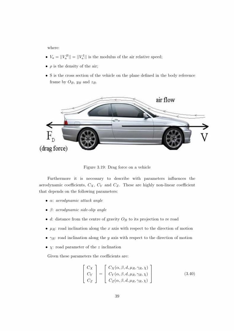
Figure 3.19: Drag force on a vehicle

Furthermore it is necessary to describe with parameters influences theaerodynamic coefficients, CX , CY and CZ . These are highly non-linear coefficientthat depends on the following parameters:

• α: aerodynamic attack angle

• β: aerodynamic side-slip angle

• d: distance from the centre of gravity OB to its projection to re road

• µR: road inclination along the x axis with respect to the direction of motion

• γR: road inclination along the y axis with respect to the direction of motion

• χ: road parameter of the z inclination

Given these parameters the coefficients are: CX

CY

CZ

=

CX(α, β, d, µR, γR, χ)

CY (α, β, d, µR, γR, χ)

CZ(α, β, d, µR, γR, χ)

(3.40)

39

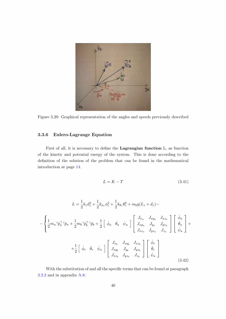
Figure 3.20: Graphical representation of the angles and speeds previously described

3.3.6 Eulero-Lagrange Equation

First of all, it is necessary to define the Lagrangian function L, as functionof the kinetic and potential energy of the system. This is done according to thedefinition of the solution of the problem that can be found in the mathematicalintroduction at page 14.

L = K − T (3.41)

L =1

2kzd

2z +

1

2kφrφ

2r +

1

2kθrθ

2r +mbg(Lz + dz)−

−

1

2mu

ip>uipu +

1

2mb

ip>bipb +

1

2

[φu θu ψu

] Jxu Jxyu Jxzu

Jxyu Jyu Jyzu

Jxzu Jyzu Jzu

φu

θu

ψu

+

+1

2

[φr θr ψu

] Jxb Jxyb JxzbJxyb Jyb JyzbJxzb Jyzb Jzb

φr

θr

ψu

(3.42)

With the substitution of and all the specific terms that can be found at paragraph3.2.2 and in appendix A.8:

40


)+


Below, it is possible to find all the Eulero-Lagrange equations one for eachvariable the appears in the lagrangian function L. The external forces related to eachvariable can be found considering zero all the other variables, with except of theconsidered one, and taking into account all the forces and torques that influencethat variable.

• ipu:

∂L

∂ ipu− ∂

∂t

∂L

∂ ipu= (mu +mb)

ipu+

+mb

[ALzφr +BLz θr + C

(dz − Lxθr

)+DLxψu

]=∑

iFw + iFa

( ipu(3) ≡ 0)

(3.44)

• dz:∂L

∂dz− ∂

∂t

∂L

∂dz= kzdz +mbg +mb

ip>uC +mbdz =

= e>z R2(−θr)R1(−φr) bFa − βzdz

( ip>uC ≡ 0)

(3.45)

• φr:

∂L

∂φr− ∂

∂t

∂L

∂φr= kφrφr +mb

ip>uLzA+[φr θr ψu

] mbL2zb

+ JxbJxybJxzb

=

= −βφr φr + e>x ( bFa × bL)

(3.46)

41

• θr:

∂L

∂θr− ∂

∂t

∂L

∂θr= kθrθr +mb

ip>uLzB −mbip>uLxC +

1

2mbA

>DLxbLzbψu+

+[φr θr ψu

] Jxybmb(L

2zb

+ L2xb

) + JybJyzb

= −βθr θr + e>y R1(−φr)( bFa × bL)

( ip>uC ≡ 0A>D ≡ −1)

(3.47)

• ψu:∂L

∂ψu− ∂

∂t

∂L

∂ψu= mb

ip>uLxD +1

2mbA

>DLxbLzb θr+

+[φr θr ψu

] JxzbJyzb

Jzb + Jzu +mbL2xb

=

e>z

[∑uτw +R2(−θr)R1(−φr)( bFa × bL)

](A>D ≡ −1)

(3.48)

• φu:

∂L

∂φu− ∂

∂t

∂L

∂φu= Jxzb ψu + Lz

2mb φr −mb cosψu dz puy + Lzmb dz φr−

+Lxmb dz ψu + +mb sinψu dz pux − Lzmb cosψu puy − Lx Lzmb ψu+

+Lzmb sinψu pux − 2Lz2mb θr ψu − 2Lzmb dz θr ψu = 0

(3.49)

42

• θu:

∂L

∂θu− ∂

∂t

∂L

∂θu= Jyzb ψu − Lxmb dz + Lx

2mb θr + Lz2mb θr − Lxmb dz ψ

2u

+mb cosψu dz pux + Lzmb dz θr +mb sinψu dz puy+

−Lx Lzmb ψ2u + Lzmb cosψu pux + Lzmb sinψu puy + 2Lz

2mb φr ψu+

+2Lzmb dz φr ψu + Lx Lzmb sinψu φr + 2Lx Lzmb cosψu ψu φr = 0

(3.50)

It is necessary to specify that for the aerodynamic forces, some de-rotations areapplied to be coherent with the main reference system. As it is possible to see fromthe equation 3.39, the aerodynamic forces, as a consequence also the torques, areexpressed in the body reference frame, while all the Euler-Lagrange equations havebeen calculated in the under-vehicle reference frame. It is also necessary to performa selection of the forces on a specific axis, because the specific Lagrangian variablesare not influenced by the forces along the three axis.

It is possible to find the the definition of these de-rotation and selections in theappendix A.9.

In order to solve this complex system of second order differential equations, itis useful to write it in the matrix form. At this point, all the symbolic matrix thathave been substituted, to have easier computation, are going to be written in theoriginal form.

mb +mu 0 Lzmb sinψu Lzmb cosψu −Lxmb sinψu 0

0 mb +mu −Lzmb cosψu Lzmb sinψu Lxmb cosψu 0

0 0 0 0 0 mbLzmb sinψu −Lzmb cosψu mbL

2z + Jxb Jxyb Jxzb 0

Lzmb cosψu Lzmb sinψu Jxyb mb(L2zb

+ L2xb

) + Jyb Jyzb −1

2mbLxbLzb 0

−Lxmb sinψu Lxmb cosψu Jxzb Jyzb −1

2mbLxbLzb Jzb + Jzu +mbL

2xb

0

dzmb sinψu + Lzmb sinψu −dzmb cosψu − Lzmb cosψu mbL2z +mbLzdz 0 Jxzb − LxLzdz 0

dzmb cosψu + Lzmb cosψu dzmb sinψu + Lzmb sinψu LxLzmb sinψu mb(L2zb

+ L2xb

) + Lzmbdz Jyzb −Lxmb

ipu(1)ipu(2)

φrθrψudz

=

∑ iFwx + iFax∑ iFwy + iFayuFaz − βz dz − kz dz −mb g

e>x ( bFa × bL) − βφr φr − kφrφr

e>y R1(−φr)( bFa × bL) − βθr θr − kθr θr

e>z

[R2(−θr)R1(−φr)( bFa × bL) +

∑u τw

]2Lz

2mb θr ψu + 2Lzmb dz θr ψuLxmb dz ψ

2u + Lx Lzmb ψ

2u − 2Lz

2mb φr ψu − 2Lzmb dz φr ψu − 2Lx Lzmb cosψu ψu φr

(3.51)

Considering that the equation in dz is independent from the others, it is possibleto take it out from the system and it solution is:

43

dz =uFaz − βz dz − kz dz − gmb

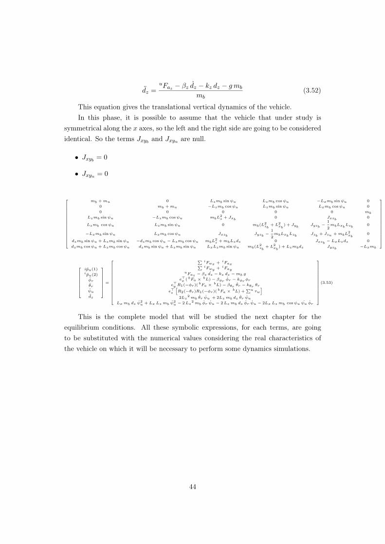
mb(3.52)

This equation gives the translational vertical dynamics of the vehicle.In this phase, it is possible to assume that the vehicle that under study is

symmetrical along the x axes, so the left and the right side are going to be consideredidentical. So the terms Jxyb and Jxyu are null.

• Jxyb = 0

• Jxyu = 0




2z + Jxb 0 Jxzb 0

Lzmb cosψu Lzmb sinψu 0 mb(L2zb

+ L2xb

) + Jyb Jyzb −1

2mbLxbLzb 0



2xb

0



+ L2xb


ipu(1)ipu(2)

φrθrψudz

=

∑ iFwx + iFax∑ iFwy + iFayuFaz − βz dz − kz dz −mb g

e>x ( bFa × bL) − βφr φr − kφrφr

e>y R1(−φr)( bFa × bL) − βθr θr − kθr θr

e>z

[R2(−θr)R1(−φr)( bFa × bL) +

∑u τw

]2Lz

2mb θr ψu + 2Lzmb dz θr ψuLxmb dz ψ

2u + Lx Lzmb ψ

2u − 2Lz

2mb φr ψu − 2Lzmb dz φr ψu − 2Lx Lzmb cosψu ψu φr

(3.53)

This is the complete model that will be studied the next chapter for theequilibrium conditions. All these symbolic expressions, for each terms, are goingto be substituted with the numerical values considering the real characteristics ofthe vehicle on which it will be necessary to perform some dynamics simulations.

44

Chapter 4

Equilibrium Analysis

In this chapter, it will be analyzed the behaviour of the proposed non-linearsystem under the equilibrium conditions. In order to do so, it is necessary to considersome simplifying assumption to describe in which kind of situation the system is goingto be analyzed.

4.1 Definition of the equilibrium condition

First of all, it is necessary to describe the trajectory along which the analysiswill be performed. It has been assumed that the car is on a point of equilibriumwhile performing an ideal turn, this means that the trajectory is perfectly round andthe speed of the vehicle is constant during the entire route.

• R = const

• VOB = const

There is also an additional kinematic condition deriving from this ideal situationthat is preferable to achieve. he βU angle is constant, this is the angle between thebow of the vehicle and the tangent to the curve, as it has been defined at paragraph3.1. As a consequence, of this kinematic condition, the first order dynamic of ψu isconstant and it depends only from the tangential speed Vtg and the radius of theturn R.

Considering the fact that the analysis is done in static conditions, this means,together with the previous consideration, that the relative angles [φr θr β], belongingto the system, are constant. Furthermore, in this situation it is considered that thesuspension are in rest position, thus lead actually to null relative angles, [φr θr].

Taking into account all these considerations, it is possible to gather that:

47

1. ψu:ψu = const(K)⇒ ψu = 0 (4.1)

2. φr:φr ⇒ φr = 0⇒ φr = 0 (4.2)

3. θr:θr = 0⇒ θr = 0⇒ θr = 0 (4.3)

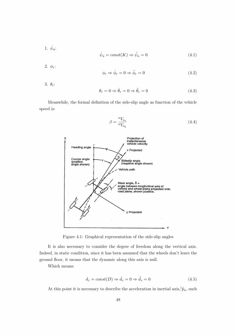
Meanwhile, the formal definition of the side-slip angle as function of the vehiclespeed is:

β =uVoxuVoy

(4.4)

Figure 4.1: Graphical representation of the side-slip angles

It is also necessary to consider the degree of freedom along the vertical axis.Indeed, in static condition, since it has been assumed that the wheels don’t leave theground floor, it means that the dynamic along this axis is null.

Which means:

dz = const(D)⇒ dz = 0⇒ dz = 0 (4.5)

At this point it is necessary to describe the acceleration in inertial axis,ipu, such

48

that the vehicle keeps the trajectory and it remains on the circle. It is important toknow the modulus of the acceleration because actually the direction is known and itis along the radius that sweeps the turn.

In this conditions, also the modulus of the acceleration depends only on thetangential speed Vtg and the radius of the turn R, according to the following formula:

|ipu| =V 2t

R(4.6)

This is valid only in case of constant speed and radius.In inertial axis, the two components are:

ipux = −V2t

Rcosα (4.7)

ipuy = −V2t

Rsinα (4.8)

Where α is a generic angle that indicates at which point of the curvilineartrajectory the vehicle is arrived. It is a generic angle considered during the rotationtaking into account the position of the vehicle with respect to the centre of thecircle, so it is function of time. While considering this representation β is the angleof projection of the acceleration.

While in tangential and radial axes, they are:

put = 0 (4.9)

pur =V 2t

R(4.10)

While considering this representation, in the tangential-radial plane, the side-slipangle β is the angle of projection of the acceleration in the inertial reference frame.

It is necessary now to express the relationship between the accelerationdecomposed along the inertial axis and it expression along the tangential and radialaxes. To do so, it is necessary first to pass through the representation in theunder-vehicle reference frame. It is possible to perform two consecutive rotationsfirst of angle β and than of angle ψu, according to the following matrices:

uRt (β) =

cosβ − sinβ 0

sinβ cosβ 0

0 0 1

(4.11)

49

iRu (ψu) =

cosψu − sinψu 0

sinψu cosψu 0

0 0 1

(4.12)

In conclusion, the relationship between the acceleration expressed in the inertialreference frame and the one expressed in the radial-tangential plane is:

ipuxy = iRu (ψu) uRt (β) putr (4.13)

A graphical representation of all these consideration can be found in figure 5.1.

Figure 4.2: Graphical representation of the vehicle accelerations according to twodifferent reference frame

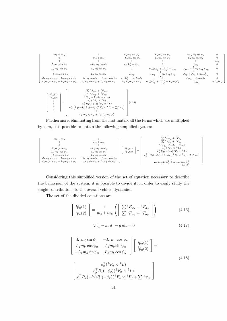
4.2 Complete model at the equilibrium conditions

Now it is necessary to go back and consider again the complete model, that canbe found in the equation 3.3.6 and gather together all the equilibrium assumptions:

• ψu = const(K)⇒ ψu = 0

• φr = θr = 0⇒ φr = θr = 0⇒ φr = θr = 0

• dz = const(D)⇒ dz = 0⇒ dz = 0

Thus leading to the following simplified set of equations:

50




2z + Jxb 0 Jxzb 0

Lzmb cosψu Lzmb sinψu 0 mb(L2zb

+ L2xb

) + Jyb Jyzb −1

2mbLxbLzb 0



2xb

0



+ L2xb


ipu(1)ipu(2)

0

0

0

0

=

∑ iFwx + iFax∑ iFwy + iFayuFaz − kz dz −mb g

e>x ( bFa × bL)

e>y R1(−φr)( bFa × bL)

e>z

[R2(−θr)R1(−φr)( bFa × bL) +

∑u τw

]0

Lxmb dz ψ2u + Lx Lzmb ψ

2u

(4.14)

Furthermore, eliminating from the first matrix all the terms which are multipliedby zero, it is possible to obtain the following simplified system:

mb +mu 0

0 mb +mu0 0

Lzmb sinψu −Lzmb cosψuLzmb cosψu Lzmb sinψu−Lxmb sinψu Lxmb cosψu

dzmb sinψu + Lzmb sinψu −dzmb cosψu − Lzmb cosψudzmb cosψu + Lzmb cosψu dzmb sinψu + Lzmb sinψu

[ipu(1)ipu(2)

]=

∑ iFwx + iFax∑ iFwy + iFayuFaz − kz dz −mb g

e>x ( bFa × bL)


e>z

[R2(−θr)R1(−φr)( bFa × bL) +

∑u τw

]0


2u

(4.15)

Considering this simplified version of the set of equation necessary to describethe behaviour of the system, it is possible to divide it, in order to easily study thesingle contributions to the overall vehicle dynamics.

The set of the divided equations are:[ipu(1)ipu(2)

]=

1

mb +mu

([ ∑iFwx + iFax∑iFwy + iFay

])(4.16)

iFaz − kz dz − gmb = 0 (4.17)

Lzmb sinψu −Lzmb cosψu

Lzmb cosψu Lzmb sinψu

−Lxmb sinψu Lxmb cosψu

[ ipu(1)ipu(2)

]=

e>x ( bFa × bL)


e>z R2(−θr)R1(−φr)( bFa × bL) +∑

uτw

(4.18)

51

[dzmb sinψu + Lzmb sinψu −dzmb cosψu − Lzmb cosψu

dzmb cosψu + Lzmb cosψu dzmb sinψu + Lzmb sinψu

][ipu(1)ipu(2)

]=

[0


2u

](4.19)

Now it is possible to study individually the behaviour of the different equation,taking into account all the necessary substitutions and simplifications.

Starting from the equations 4.16:[ipu(1)ipu(2)

]=

1

mb +mu


])(4.20)

Where the forces of the wheels and the aerodynamic forces needs to be expressedin the inertial reference frame, while they have been defined in the paragraph3.3.5 in a different one, in the wheel reference frame and the body reference framerespectively. So they need to be rotated according to the following formulas:

iFa = iRuuRb

bFa (4.21)

iFw = iRuuRwi

wiFwi (4.22)

It is also necessary to substitute in the previous equation, 4.16, the relationshipcoming from the formula 4.13.

iRu (ψu) uRt (β) putr =1

mb +mu


])(4.23)

It is possible to see that there is the same rotation matrix on both side, betweenthe inertial reference frame and the under-vehicle, that it means that it is possibleto simplify it. As a consequence it remains only the the one in β that is the one ofinterest.

uRt (β) putr =1

mb +mu

([ ∑uFwx + uFax∑uFwy + uFay

])(4.24)

where all the terms are expressed in the under-vehicle reference frame.At this point it is necessary to isolate the variable of interest, that are the wheel

forces, arriving to the following formula:

52

∑uFwi = (mb +mu) uRt (β) putr − uFa (4.25)

This equation tells how the forces on the wheel varies as function of the side slipangle. These are centripetal forces that have the same direction of the accelerationof the vehicle projected with β.

Afterwards, it is necessary to analyze the third set of equations, 4.26:

Lzmb sinψu −Lzmb cosψu

Lzmb cosψu Lzmb sinψu

−Lxmb sinψu Lxmb cosψu

[ ipu(1)ipu(2)

]=

e>x ( bFa × bL)


e>z R2(−θr)R1(−φr)( bFa × bL) +∑

uτw

(4.26)

In this case, it is necessary to substitute the accelerations with the samerelationship used before, the one coming from the equation 4.13. Considering thematrix that pre-multiplies the acceleration now is multiplied by the rotational matrixiRu (ψu), a lot of simplifications come as a consequence.

It is also necessary to take into account, on the right side of the equation, whichare the cross product between the aerodynamic forces and there own arms, togetherwith all the de-rotation matrices and the selection vectors, that have been defined inthe appendix A.9. All these consideration together leads to the following simplifiedrelationship:

0 −Lzmb 0

Lzmb 0 0

0 Lxmb 0

uRt (β) putr =

bFay

bLzbFaz

bLx − bFaxbLz

− bFazbLx +

∑uτw

(4.27)

The last equation gives the yaw dynamics of the system.

Where the definition of the torques forces is the following one:

uτw = ( uRw(δw)wFw)× uLw = uFw × uLw = −S( uLw) uFw (4.28)

53

S( uLw) =

0 − bLz 0bLz 0 − bLx

0 bLx 0

(4.29)

uτw = −S( uLw) uFw = −

0 − bLz 0bLz 0 − bLx

0 bLx 0

uFwxuFwyuFwz

=

= −

− bLzuFwy

bLzuFwx − bLx

uFwzbLx

uFwz

=

bLz

uFwybLx

uFwz − bLzuFwx

− bLxuFwz

(4.30)

All the calculation done to consider the de-rotation matrices and selection of thespecific torques con be found in the appendix A.10.

The last set of equation is given by the equation, 4.19:



][ipu(1)ipu(2)

]=

[0


2u

](4.31)

As in the previous cases, the substitution of the acceleration expressed inthe tangential reference frame, according to the relationship 4.13, leads to somesimplification:

0 −1 0

1 0 0

0 0 0

uRt (β) putr =

[0

Lx ψ2u

](4.32)

The calculation on how the terms have been simplified can be found in theappendix A.11.

The complete set of equation in which it has been explicit the terms uRt (β) andputr , according to the definitions given at page 49, are the following:

54

[ ∑uFwxi∑uFwyi

]= (mb +mu)

[cosβ − sinβ

sinβ cosβ

] 0

V 2t

R

− [ uFaxuFay

](4.33)

iFaz − kz dz − gmb = 0 (4.34)

0 −Lzmb 0

Lzmb 0 0

0 Lxmb 0

cosβ − sinβ 0

sinβ cosβ 0

0 0 1

0

V 2tR

0

=

bFay

bLzbFaz

bLx − bFaxbLz

− bFazbLx −

∑bLx

uFwz

(4.35)

0 −1 0

1 0 0

0 0 0

cosβ − sinβ 0

sinβ cosβ 0

0 0 1

0

V 2tR

0

=

0

Lx ψ2u

0

(4.36)

The equation 4.46 gives the vertical equilibrium of the system. An additionalconstrain needs to be taken into account, i.e. the equilibrium of the torques of thesystem. Since the system is in static conditions, the equilibrium is give for fixed rolland pitch angle. This is given according to the following definitions:

∑uτ =

∑uτwi + uτa + uτg = 0 (4.37)

∑uτwi =

∑( uRwi(δwi)

wFwi)× uLwi (4.38)

uτa = ( uRbbFa)× uLa (4.39)

uτg = ( uRiigmb)× uLm (4.40)

With the arm uLm obtained from the difference of the position of theunder-vehicle and the body parts:

uLm = upb − upu =u

0

0

dz

+ uRb(φr, θr)b

Lx

0

Lz

(4.41)

It is necessary to take into account only the equations that gives the roll and

55

pitch dynamics, taking into account the cross-product:

∑bLz

uFwy + uLazuFay + uLmz

igmb = 0 (4.42)

∑( bLx

uFwz − bLzuFwx) + bLax

uFaz − bLazuFax + bLmx

igmb − bLmzigmb = 0

(4.43)The final list of equations is:

uFwx1 + uFwx2 + uFwx3 + uFwx4 = −(mb +mu) sinβV 2t

R− uFax (4.44)

uFwy1 + uFwy2 + uFwy3 + uFwy4 = (mb +mu) cosβV 2t

R− uFay (4.45)

iFaz − kz dz − gmb = 0 (4.46)

− Lzmb cosβV 2t

R= bFay

bLz (4.47)

− Lzmb sinβV 2t

R= bFaz

bLx − bFaxbLz (4.48)

∑bLx

uFwz = − bFazbLx − Lxmb cosβ

V 2t

R(4.49)

− cosβV 2t

R= 0 (4.50)

− sinβV 2t

R= Lx ψ

2u (4.51)

∑bLz

uFwy = − uLazuFay − uLmz

igmb (4.52)

∑( bLx

uFwz − bLzuFwx) = − bLax

uFaz + bLazuFax − bLmx

igmb + bLmzigmb

(4.53)

56

Chapter 5

Conclusion

At this point, with all the gathered equations, it is possible to describe thefeed-forward law, that given the forces and torques on the vehicle, that gives thewheel force that are applied to the ground.

The unknown of the problem, since the beginning, are forces acting on thewheels. From the complete system, given at the equation 3.3.6, it is possible to seethat there are 8 equations with 12 unknown. This means that the problem has aninfinite number of solution. Indeed this is an hyperstatic problem because it comesfrom an undersized system.

In order to solve the problem, it is necessary to select one of the infinite solutionsand in this case it has been decided to exploit the one that minimize the norm. Todo so, it is necessary to calculate the Moore-Penrose pseudo inverse, that incase of a matrix that has linearly independent rows, is defined in the following way:

A+ = A∗(A ·A∗)−1 (5.1)

This is a right pseudoinverse, as A · A+ = 1 for a non injective problem. Thisis a non injective matrix because the A matrix belongs to the space Km×n wheren > m.

For this specific problem, the A is the following one:

cos δwx1− sin δwx1

0 cos δwx2− sin δwx2



0

sin δwx1cos δwx1

0 sin δwx2cos δwx2



0

0 0 uLx1 0 0 uLx2 0 0 uLx3 0 0 uLx4uLz1 sin δwx1

uLz1 cos δwx10 uLz2 sin δwx2



uLz4 cos δwx40

−uLz1 cos δwx1uLz1 sin δwx1

uLx1 −uLz2 cos δwx2uLz2 sin δwx2



uLx4

(5.2)

This is obtained from the final system of chapter 4, substituting all the specificrotation matrix of each wheel to have all the terms in the under-vehicle reference

59

frame. While the vector bL is coincident with uL if the relative angles φr and θr arenull.

Figure 5.1: Definition of the wheel numeration

The previous matrix can be simplified considering the fact that only the frontwheel are steering wheels. This consideration gives:

• δwx3 = 0

• δwx4 = 0

The simplified matrix is:

cos δwx1− sin δwx1


0 1 0 0 1 0 0

sin δwx1cos δwx1


0 0 1 0 0 1 0

0 0 uLx1 0 0 uLx2 0 0 uLx3 0 0 uLx4uLz1 sin δwx1


uLz2 cos δwx20 0 1 0 0 1 0

−uLz1 cos δwx1uLz1 sin δwx1


uLx2 −1 0 uLx3 −1 0 uLx4

(5.3)

60

Acknowledgements

Innanzitutto un immenso e vivissimo ringraziamento va al professor NicolaMimmo, che in tutti questi mesi mi ha supportata ed aiutata. La sua disponibilità eil suo collaborazione sono state per me fonte di forza e determinazione per portare altermine questo lavoro di tesi, nonostante le difficoltà dovute alla mancanda di tempoe all’inizio del lavoro.

Un particolare ringraziamento va al professore Riccardo Rovatti, che all’inizio diquesto cammino si è preso a cuore la mia iscrizione alla magistrale e mi ha aiutata acercare di realizzare un sogno nel cassetto. Vorrei inoltre ringraziare tutti i professoriincotrati in questo tortuoso cammino burocratico, la loro gentilezza e disponibilità èstata ammirevole.

Vorrei poi ringraziare la mia famiglia, che in questi anni mi ha sostenuta in ognidifficoltà e situazione, permettendomi di vivere un’esperienza utile e formativa comel’Erasmus. Loro sono sempre stati al mio fianco, insegnandomi il valore dell’impegnoe della dedizione.

In fine, ma non per ultimi, vorrei ringraziare tutti i miei amici che, durantequesto percorso, mi hanno aiutata a credere in me stessa e a non dubitare delle miecapacità.

63

64 CHAPTER 5. CONCLUSION

Appendix A

Calculations

A.1 Complete relative rotational matrix

uRb(Θr) = R1(φr)R2(θr)R3(ψr) =

=

cosψr cos θr cos θr sinψr − sin θr

cosψr sinφr sin θr − cosφr sinψr cosφr cosψr + sinφr sinψr sin θr cos θr sinφr

sinφr sinψr + cosφr cosψr sin θr cosφr sinψr sin θr − cosψr sinφr cosφr cos θr

(A.1)

A.2 Complete under-vehicle rotational matrix

iRu(Θu) = R>3 (ψu)R>2 (θu)R>1 (φu) =

=

cosψu cos θu cosψu sinφu sin θu − cosφu sinψu sinφu sinψu + cosφu cosψu sin θu

cos θu sinψu cosφu cosψu + sinφu sinψu sin θu cosφu sinψu sin θu − cosψu sinφu

− sin θu cos θu sinφu cosφu cos θu

(A.2)

65

66 APPENDIX A. CALCULATIONS

A.3 Complete navigation rotational matrix

URN (γU , βU ) =

cosβU cos γU − cos γU sinβU sin γU

sinβU cosβU 0

− cosβU sin γU sinβU sin γU cos γU

(A.3)

A.4 Complete i-th wheel reference frame

URWi (φWi , δWi) =

cos δWi − sin δWi 0

cosφWi sin δWi cos δWi cosφWi − sinφWi

sin δWi sinφWi cos δWi sinφWi cosφWi

(A.4)

A.5 Vehicle position

ipb = ipu+

(sinφu sinψu + cosφu cosψu sin θu) (dz − Lx sin θr + Lz cosφr cos θr) +

+ cosψu cos θu (Lx cos θr + Lz cosφr sin θr) + Lz sinφr (cosφu sinψu − cosψu sinφu sin θu)

− (cosψu sinφu − cosφu sinψu sin θu) (dz − Lx sin θr + Lz cosφr cos θr) +

+ cos θu sinψu (Lx cos θr + Lz cosφr sin θr)− Lz sinφr (cosφu cosψu + sinϕu sinψu sin θu)

cosφu cos θu (dz − Lx sin θr + Lz cosφr cos θr)−+ sin θu (Lx cos θr + Lz cosφr sin θr)− Lz cos θu sinφr sinφu

(A.5)

A.6. SMALL ANGLE APPROXIMATION 67

A.6 Small angle approximation

ipb ≈i pu+

(sinφu sinψu + cosφu cosψu sin θu) (dz − Lx θr + Lz) +

+ cosψu cos θu (Lx + Lz θr) + Lz φr (cosφu sinψu − cosψu sinφu sin θu)

− (cosψu sinφu − cosφu sinψu sin θu) (dz − Lx θr + Lz) +

+ cos θu sinψu (Lx + Lz θr)− Lz φr (cosφu cosψu + sinφu sinψu sin θu)

cosφu cos θu (dz − Lx θr + Lz)−+ sin θu (Lx + Lz θr)− Lz φr cos θu sinφu

(A.6)

A.7 Simplified position equation

ipb ≈ ipu +

(sinφu sinψu + cosφu cosψu sin θu)

− (cosψu sinφu − cosφu sinψu sin θu)

cosφu cos θu

(dz − Lx θr + Lz) +

+

cosψu cos θu

cos θu sinψu

− sin θu

(Lx + Lz θr) +

(cosφu sinψu − cosψu sinφu sin θu)

− (cosφu cosψu + sinφu sinψu sin θu)

− cos θu sinφu

(Lz φr)

(A.7)

A.8 Partial derivatives used in the position computation

∂A

∂φu=

sinψu cosφu − cosψut sin θu sinφu

− cosψu cosφu − sinψu sin θu sinφu

− cos θu sinφu

(A.8)

∂A

∂θu=

cosφu cosψu cos θu

cosφu sinψu cos θu

− cosφu sin θu

(A.9)


∂A

∂ψu=

sinφu cosψu − cosφu sin θu sinψu

sinφu sinψu + cosφu sin θu cosψu

0

(A.10)

∂B

∂φu=

0

0

0

(A.11)

∂B

∂θu=

− cosψu sin θu

− sinψu sin θu

− cos θu

(A.12)

∂B

∂ψu=

− cos θu sinψu

cos θu cosψu

0

(A.13)

∂C

∂φu=

− sinψu sinφu − cosψu sin θu cosφu

cosψu sinφu + sinψu sin θu cosφu

0

(A.14)

∂C

∂θu=

− cosψu sinφu cos θu

sinφu sinψu cos θu

sinψu sin θu

(A.15)

∂C

∂ψu=

sinφu cosψu − cosφu sin θu sinψu

sinφu sinψu + cosϕu sin θu cosψu

0

(A.16)

A.9 Derotation and selection

1. Selections:ex = (1; 0; 0) ey = (0; 1; 0) ez = (0; 0; 1) (A.17)

2. De-rotation only along the first axis xB:

R1(−φr) = R>1 (φr) =

1 0 0

0 cosφr − sinφr

0 sinφr cosφr

(A.18)

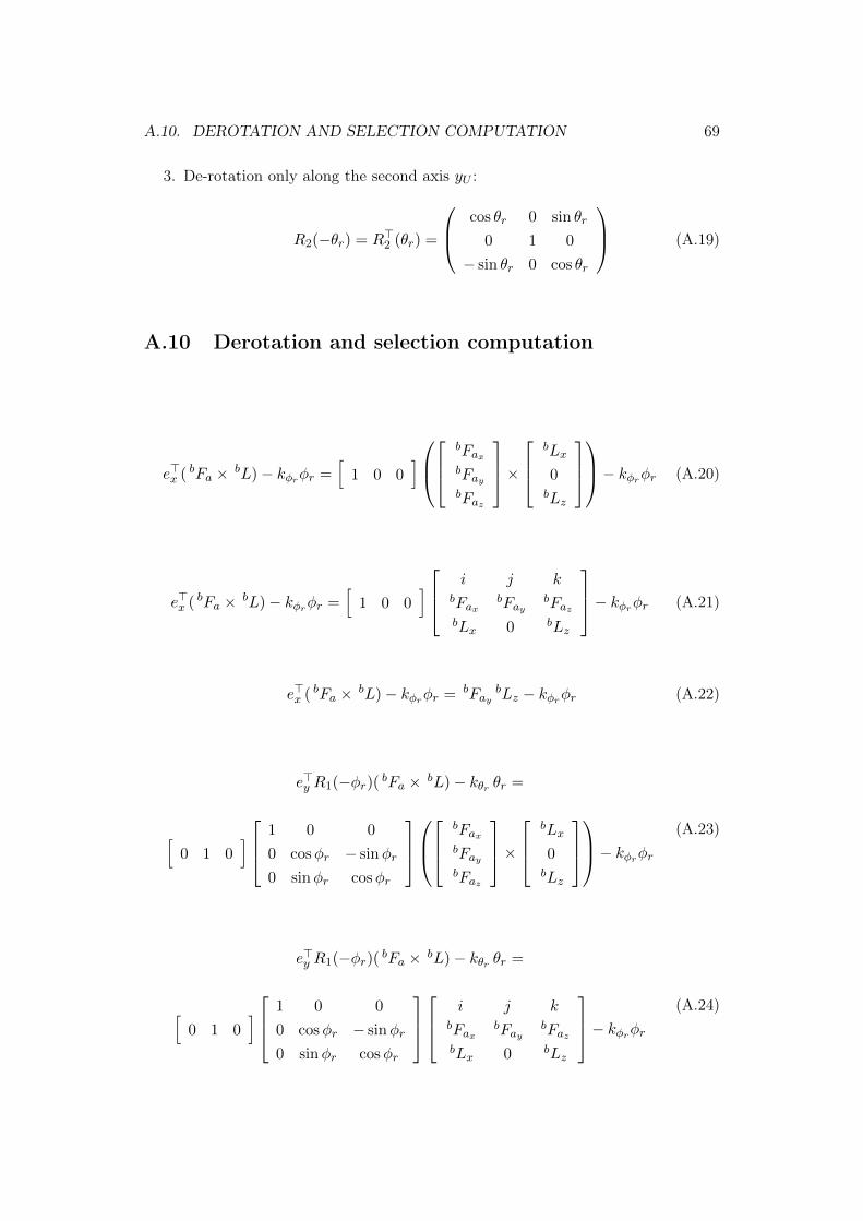
A.10. DEROTATION AND SELECTION COMPUTATION 69

3. De-rotation only along the second axis yU :

R2(−θr) = R>2 (θr) =

cos θr 0 sin θr

0 1 0

− sin θr 0 cos θr

(A.19)

A.10 Derotation and selection computation

e>x ( bFa × bL)− kφrφr =[

1 0 0]

bFaxbFaybFaz

×

bLx

0bLz

− kφrφr (A.20)

e>x ( bFa × bL)− kφrφr =[

1 0 0] i j k

bFaxbFay

bFazbLx 0 bLz

− kφrφr (A.21)

e>x ( bFa × bL)− kφrφr = bFaybLz − kφrφr (A.22)

e>y R1(−φr)( bFa × bL)− kθr θr =

[0 1 0

] 1 0 0

0 cosφr − sinφr

0 sinφr cosφr

bFaxbFaybFaz

×

bLx

0bLz

− kφrφr (A.23)


[0 1 0

] 1 0 0

0 cosφr − sinφr

0 sinφr cosφr

i j k

bFaxbFay

bFazbLx 0 bLz

− kφrφr (A.24)



[0 1 0

] 1 0 0

0 1 −φr0 φr 1

bLzuFay

bLxuFaz − bLz

uFax

− bLxuFaz

− kφrφr (A.25)

e>y R1(−φr)( bFa× bL)− kθr θr = bFazbLx− bLz

uFax + bLxuFazφr− kφrφr (A.26)

e>z R2(−θr)R1(−φr)( bFa × bL) =

[0 0 1

] cos θr 0 sin θr

0 1 0


1 0 0

0 cosφr − sinφr

0 sinφr cosφr

bFaxbFaybFaz

×

bLx

0bLz

(A.27)


[0 0 1

] cos θr 0 sin θr

0 1 0


1 0 0

0 cosφr − sinφr

0 sinφr cosφr

i j k

bFaxbFay

bFazbLx 0 bLz

(A.28)


[0 0 1

] 1 0 θr

0 1 0

−θr 0 1

1 0 0

0 1 −φr0 φr 1

bLzuFay

bLxuFaz − bLz

uFax

− bLxuFaz

(A.29)

A.11. SIMPLIFICATIONS 71


[0 0 1

] 1 0 θr

0 1 0

−θr 0 1

bFaybLz

bLxuFaz − bLz

uFax + bLxuFazφr(

bLxuFaz − bLz

uFax)φr − bLx

uFaz

(A.30)

e>z R2(−θr)R1(−φr)( bFa× bL) = − bFaybLz θr+

(bLx

uFaz − bLzuFax

)φr− bLx

uFaz

(A.31)

A.11 Simplifications



][ipu(1)ipu(2)

]=

=

[0


2u

](A.32)

[(dz + Lz)mb sinψu −(dz + Lz)mb cosψu

(dz + Lz)mb cosψu (dz + Lx)mb sinψu

][ipu(1)ipu(2)

]=

[0


2u

](A.33)

(dz + Lz)mb

[sinψu − cosψu

cosψu sinψu

][ipu(1)ipu(2)

]=

[0

Lx ψ2umb(dz + Lz)

](A.34)

[sinψu − cosψu

cosψu sinψu

][ipu(1)ipu(2)

]=

[0

Lx ψ2u

](A.35)

[sinψu − cosψu

cosψu sinψu

][ipu(1)ipu(2)

]=

[0

Lx ψ2u

](A.36)


sinψu − cosψu 0

cosψu sinψu 0

0 0 0

cosψu − sinψu 0

sinψu cosψu 0

0 0 1

uRt (β) putr =

[0

Lx ψ2u

](A.37) 0 −1 0

1 0 0

0 0 0

uRt (β) putr =

[0

Lx ψ2u

](A.38)

Appendix B

Matlab™Code

B.1 Variables definition

clear allclose allclc

syms t real %timesyms x y z real %generic variablessyms m_u m_b %massessyms L_x L_z %armsyms J_xu J_yu J_zu J_xyu J_xzu J_yzu %under−vehicle inertiasyms J_xb J_yb J_zb J_xyb J_xzb J_yzb %body inertiassyms F_ax F_ay F_az %aerodynamic forcessyms F_wx F_wy F_wz %wheel forcessyms tau_wx tau_wy tau_wz %wheel momentasyms k_z k_pr k_tr k_x k_y %elastic constantssyms B_pr B_tr B_z %damping constantssyms d_z(t) %vertical movementsyms d %vertical movement derivativesyms g %gravitational constantsyms tau_w %wheel momentasyms de %a determinant

syms phi_r(t) theta_r(t) real %relative anglessyms dphi_r(t) dtheta_r(t) real %rotational speed of the bodysyms phi_u(t) theta_u(t) psi_u(t) real %undervehicle anglesyms dphi_u(t) dtheta_u(t) dpsi_u(t) real %rotational speed of the undervehiclesyms p_x(t) p_y(t) real %undervehicle positionssyms dp_x(t) dp_y(t) real %undervehicle speeds

73

74 APPENDIX B. MATLAB™CODE

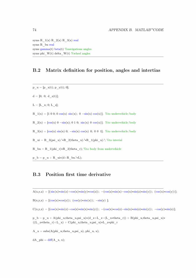
syms R_1(x) R_2(x) R_3(x) realsyms R_bu realsyms gamma(t) beta(t) %navigations anglessyms phi_W(t) delta_W(t) %wheel angles

B.2 Matrix definition for position, angles and intertias

p_u = [p_x(t); p_y(t); 0];

d = [0; 0; d_z(t)];

L = [L_x; 0; L_z];

R_1(x) = [1 0 0; 0 cos(x) sin(x); 0 −sin(x) cos(x) ]; %to undervehicle/body

R_2(x) = [cos(x) 0 −sin(x); 0 1 0; sin(x) 0 cos(x) ]; %to undervehicle/body

R_3(x) = [cos(x) sin(x) 0; −sin(x) cos(x) 0; 0 0 1]; %to undervehicle/body

R_ui = R_3(psi_u).'∗R_2(theta_u).'∗R_1(phi_u).'; %to interial

R_bu = R_1(phi_r)∗R_2(theta_r); %to body from undervehicle

p_b = p_u + R_ui∗(d+R_bu.'∗L);

B.3 Position first time derivative

A(x,y,z) = [(sin(x)∗sin(z)+cos(x)∗sin(y)∗cos(z)); −(cos(z)∗sin(x)−cos(x)∗sin(z)∗sin(y)) ; (cos(x)∗cos(y)) ];

B(x,y,z) = [(cos(z)∗cos(y)) ; (cos(y)∗sin(z)) ; −sin(y) ];

C(x,y,z) = [(cos(x)∗sin(z)−cos(z)∗sin(x)∗sin(y)) ; −(cos(x)∗cos(z)−sin(x)∗sin(z)∗sin(y)) ; −cos(y)∗sin(z) ];

p_b = p_u + A(phi_u,theta_u,psi_u)∗(d_z+L_z−(L_x∗theta_r)) + B(phi_u,theta_u,psi_u)∗((L_z∗theta_r)+L_x) + C(phi_u,theta_u,psi_u)∗L_z∗phi_r

A_x = subs(A(phi_u,theta_u,psi_u), phi_u, x);

dA_phi = diff(A_x, x);

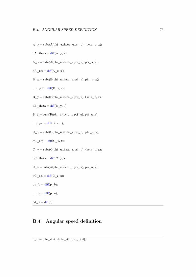
B.4. ANGULAR SPEED DEFINITION 75

A_y = subs(A(phi_u,theta_u,psi_u), theta_u, x);

dA_theta = diff(A_y, x);

A_z = subs(A(phi_u,theta_u,psi_u), psi_u, x);

dA_psi = diff(A_z, x);

B_x = subs(B(phi_u,theta_u,psi_u), phi_u, x);

dB_phi = diff(B_x, x);

B_y = subs(B(phi_u,theta_u,psi_u), theta_u, x);

dB_theta = diff(B_y, x);

B_z = subs(B(phi_u,theta_u,psi_u), psi_u, x);

dB_psi = diff(B_z, x);

C_x = subs(C(phi_u,theta_u,psi_u), phi_u, x);

dC_phi = diff(C_x, x);

C_y = subs(C(phi_u,theta_u,psi_u), theta_u, x);

dC_theta = diff(C_y, x);

C_z = subs(A(phi_u,theta_u,psi_u), psi_u, x);

dC_psi = diff(C_z, x);

dp_b = diff(p_b);

dp_u = diff(p_u);

dd_z = diff(d);

B.4 Angular speed definition

a_b = [phi_r(t); theta_r(t); psi_u(t)];


a_u = [phi_u(t); theta_u(t); psi_u(t)];

w_b = diff(a_b);

w_u = diff(a_u);

B.5 Kinetic and potential energy

J_b = [J_xb J_xyb J_xzb; J_xyb J_yb J_yzb; J_xzb J_yzb J_zb];

J_u = [J_xu J_xyu J_xzu; J_xyu J_yu J_yzu; J_xzu J_yzu J_zu];

T = ((1/2)∗m_u∗(dp_u.'∗dp_u)) + ((1/2)∗m_b∗(dp_b.'∗dp_b)) +((1/2)∗w_b.'∗J_b∗w_b) + ((1/2)∗w_u.'∗J_b∗w_u);

K = ((1/2)∗k_z∗d_z^2) + ((1/2)∗k_pr∗phi_r^2) + ((1/2)∗k_tr∗theta_r^2) + m_b∗g∗(L_z+d_z);

L = K − T;

B.6 Euler-Lagrange equations

L_pux = subs(L, p_u(1), x);dL_pux = diff(L_pux,x);dL_pux = subs(dL_pux, x, p_u(1));

L_puy = subs(L, p_u(2), x);dL_puy = diff(L_puy,x);dL_puy = subs(dL_puy, x, p_u(2));

L_dpux = subs(L, dp_u(1), x);dL_dpux = diff(L_dpux, x);dL_dpux = subs(dL_dpux, x, dp_u(1));ddL_dpux = diff(dL_dpux);

L_dpuy = subs(L, dp_u(2), x);dL_dpuy = diff(L_dpuy, x);dL_dpuy = subs(dL_dpuy, x, dp_u(2));ddL_dpuy = diff(dL_dpuy);

B.6. EULER-LAGRANGE EQUATIONS 77

L_dz = subs(L, d_z, x);dL_dz = diff(L_dz, x);dL_dz = subs(dL_dz, x, d_z);

L_ddz = subs(L, dd_z(3), x);dL_ddz = diff(L_ddz, x);dL_ddz = subs(dL_ddz, x, dd_z(3));ddL_ddz = diff(dL_dz);

L_phr = subs(L, phi_r, x);dL_phr = diff(L_phr, x);dL_phr = subs(dL_phr, x, phi_r);

L_dphr = subs(L, w_b(1), x);dL_dphr = diff(L_dphr, x);dL_dphr = subs(dL_dphr, x, w_b(1));ddL_dphr = diff(dL_dphr);

L_thr = subs(L, theta_r, x);dL_thr = diff(L_thr, x);dL_thr = subs(dL_thr, x, theta_r);

L_dthr = subs(L, w_b(2), x);dL_dthr = diff(L_dthr, x);dL_dthr = subs(dL_dthr, x, w_b(2));ddL_dthr = diff(dL_dthr);

L_phu = subs(L, phi_u, x);dL_phu = diff(L_phu, x);dL_phu = subs(dL_phu, x, phi_u);

L_dphu = subs(L, w_u(1), x);dL_dphu = diff(L_dphu, x);dL_dphu = subs(dL_dphu, x, w_u(1));ddL_dphu = diff(dL_dphu);

L_thu = subs(L, theta_u, x);dL_thu = diff(L_thu, x);dL_thu = subs(dL_thu, x, theta_u);

L_dthu = subs(L, w_u(2), x);dL_dthu = diff(L_dthu, x);dL_dthu = subs(dL_dthu, x, w_u(2));ddL_dthu = diff(dL_dthu);


L_psu = subs(L, psi_u, x);dL_psu = diff(L_psu, x);dL_psu = subs(dL_psu, x, psi_u);

L_dpsu = subs(L, w_u(3), x);dL_dpsu = diff(L_dpsu, x);dL_dpsu = subs(dL_dpsu, x, w_u(3));ddL_dpsu = diff(dL_dpsu);

B.7 Symplified Euler-Lagrange equations

phi_u = 0;theta_u = 0;

NdL_pux = subs(dL_pux);

NdL_puy = subs(dL_puy);

NddL_dpux = subs(ddL_dpux);

NddL_dpuy = subs(ddL_dpuy);

NdL_dz = subs(dL_dz);

NddL_ddz = subs(ddL_ddz);

NdL_phr = subs(dL_phr);

NddL_dphr = subs(ddL_dphr);

NdL_thr = subs(dL_thr);

NddL_dthr = subs(ddL_dthr);

NdL_phu = subs(dL_phu);

NddL_dphu = subs(ddL_dphu);

NdL_thu = subs(dL_thu);

NddL_dthu = subs(ddL_dthu);

B.8. ADDITIONAL COMPLETE ROTATIONAL MATRICES 79

%NdL_psu = subs(dL_psu);

%NddL_dpsu = subs(ddL_dpsu);

B.8 Additional complete rotational matrices

R_ti = R_3(psi_u).'∗R_3(beta).';

R_nu = R_2(gamma).'∗R_3(beta).';

R_Wu = R_1(phi_W).'∗R_3(delta_W).';

Bibliography

Euler–Lagrange equation. URL https://en.wikipedia.org/wiki/Euler%

E2%80%93Lagrange_equation.

Lagrangian mechanics. URL https://en.wikipedia.org/wiki/

Lagrangian_mechanics.

Inverted pendulum. URL https://en.wikipedia.org/wiki/Inverted_

pendulum.

Frame of reference. URL https://en.wikipedia.org/wiki/Frame_of_

reference.

Rigid body. URL https://en.wikipedia.org/wiki/Rigid_body.

J. P. Alberto Parra, Asier Zubizarreta and M. Dendaluce. Intelligent TorqueVectoring Approach for Electric Vehicles with Per-Wheel Motors. ComplexityVolume 2018, Article ID 7030184, 14 pages. URL https://www.hindawi.

com/journals/complexity/2018/7030184/.

D. Morin. The Lagrangian Method. URL http://www.people.fas.harvard.

edu/~djmorin/chap6.pdf.

D. L. M. William F. Milliken. Race cars vehicle dynamics. SAE International.

Sorted in alphabetic order

81

https://en.wikipedia.org/wiki/Euler%E2%80%93Lagrange_equation

https://en.wikipedia.org/wiki/Euler%E2%80%93Lagrange_equation

https://en.wikipedia.org/wiki/Lagrangian_mechanics

https://en.wikipedia.org/wiki/Lagrangian_mechanics

https://en.wikipedia.org/wiki/Inverted_pendulum

https://en.wikipedia.org/wiki/Inverted_pendulum

https://en.wikipedia.org/wiki/Frame_of_reference

https://en.wikipedia.org/wiki/Frame_of_reference

https://en.wikipedia.org/wiki/Rigid_body

https://www.hindawi.com/journals/complexity/2018/7030184/

https://www.hindawi.com/journals/complexity/2018/7030184/

http://www.people.fas.harvard.edu/~djmorin/chap6.pdf

http://www.people.fas.harvard.edu/~djmorin/chap6.pdf

82 BIBLIOGRAPHY

List of Figures

1.1 Formula E MercedesEQ car for the season 2019/20 . . . . . . . . . . 91.2 Electric All-Wheel drive architecture versus an mechanical all wheel

drive . . . . . . . . . . . . . . . . . . . . . . . . . . . . . . . . . . . . 10

3.1 Definition of the Body and Under-Vehicle systems . . . . . . . . . . 193.2 Definition of the Inertial reference frame . . . . . . . . . . . . . . . . 203.3 Definition of the Body reference frame . . . . . . . . . . . . . . . . . 213.4 Definition of the Under-vehicle reference frame . . . . . . . . . . . . 223.5 Definition of the Navigation reference frame . . . . . . . . . . . . . . 223.6 Definition of the i-th wheel reference frame . . . . . . . . . . . . . . . 233.7 Sequence of rotations used to pass from F1 to F2 . . . . . . . . . . . 243.8 Schematic of a cart inverted pendulum . . . . . . . . . . . . . . . . . 263.9 Schematic of the proposed system . . . . . . . . . . . . . . . . . . . . 273.10 Not allowed relative rotation . . . . . . . . . . . . . . . . . . . . . . . 303.11 Camber angle examples . . . . . . . . . . . . . . . . . . . . . . . . . 313.12 Weight distribution of the vehicle . . . . . . . . . . . . . . . . . . . . 323.14 Free body diagram of a driven wheel represented in two dimension . 343.15 Longitudinal friction coefficient at various longitudinal slip . . . . . . 363.16 Longitudinal friction coefficient for various road conditions . . . . . . 363.17 Rolling resistance as function of the vehicle speed . . . . . . . . . . . 363.18 Wheel forces . . . . . . . . . . . . . . . . . . . . . . . . . . . . . . . . 373.19 Drag force on a vehicle . . . . . . . . . . . . . . . . . . . . . . . . . . 393.20 Graphical representation of the angles and speeds previously described 40

4.1 Graphical representation of the side-slip angles . . . . . . . . . . . . 484.2 Graphical representation of the vehicle accelerations according to two

different reference frame . . . . . . . . . . . . . . . . . . . . . . . . . 50

5.1 Definition of the wheel numeration . . . . . . . . . . . . . . . . . . . 60

83

84 LIST OF FIGURES

List of Tables

3.1 Summary of all the required coordinate transformation, rotationmatrices and angles . . . . . . . . . . . . . . . . . . . . . . . . . . . . 25

85

study of the torque vectoring control problem

Documents