study on downside risk of demand and cost behavior …

ABSTRACT

Our study verifies cost behavior of public sector organizations by empirical techniques. First is to clarify that cost behavior of the public sector is not clear enough up to now. Second is to verify the relation between market share level and cost behavior. Last is to clarify how business managers have carried out cost management against the downside risk of demand. We used 39,803 financial data of local public enterprises of 4,342 businesses for 15 years from 1999 to 2013 for analysis. Some local public enterprises have a market share exceeding 90%. As a result of the analysis, sticky costs were confirmed throughout the local public enterprises. However, the sticky costs were confirmed regardless of the degree of monopoly. Therefore, the market share was confirmed to have no influence on cost behavior of local public enterprises. And it became clear that sticky costs strengthened cost behavior of the local public enterprises since 2006. From this fact, in the situation in which the downside risk of demand rose, it was confirmed that the local public enterprise managers could not adjust capacity due to their high fixed cost structure.

Keywords: local public enterprises, sticky costs, downside risk of demand, market share, population estimation scenarios

STUDY ON DOWNSIDE RISK OF DEMAND AND COST BEHAVIOR OF LOCAL PUBLIC ENTERPRISES: VERIFICATION OF LOCAL

PUBLIC ENTERPRISE MANAGER’S DECISION MAKING BASED ON A POPULATION ESTIMATE

SCENARIO IN THE FUTUREShoichiro Hosomi and Shohei Nagasawa*

Graduate School of Social Science, Tokyo Metropolitan University, Japan

E-mail : [email protected], [email protected]

ARTICLE InFO

Article History: Received: 10 December 2017Accepted: 15 February 2018Published: 30 April 2018

22

Asia-Pacific Management Accounting Journal, Volume 13 Issue 1

INTRODUCTION

In the last few decades, empirical research on cost behavior has developed mainly in the private sector. Anderson et al. (2003) empirically clarified that the decreased rate in cost when the activity amount decreases is small compared to the increased rate of cost when the activity amount increases, and named this phenomenon as sticky costs. Afterwards, it has been clarified empirically that cost does not change proportionally (Subramaniam and Weidenmier, 2003; Calleja et al., 2006; Weiss, 2010; Banker and Byzalov, 2014; etc.).

On the other hand, there are very few research on cost behavior in the public sector (Bradbury & Scott, 2014; Cohen et al., 2014; Holzhacker et al., 2015). Some prior studies explain that the reason is caused by the fact that accounting methods are different (Kama and Weiss, 2013; Shust and Weiss, 2014). However, in public sector organizations such as national and local governments and public enterprises, cost management is essential as well as for-profit enterprises. This is because it is indispensable for public sector organizations to conduct efficient management and cost reduction efforts in carrying out sustainable public services. Therefore, we think that cost management is also important in public institutions.

In this research, we focused on local public enterprises among public sector organizations. The local public enterprises adopt the same accounting standards and accounting treatment as for-profit enterprises though they are one of the public sector organizations. For this reason, it clears the issue of differences in accounting methods pointed out by Kama and Weiss (2013) and Shust and Weiss (2014).

In this context, in Nagasawa and Hosomi (2016) that analyzes cost behavior of the Japanese local public enterprises, we clarified that there are sticky costs and an anti-sticky costs from 1979 to 1998 as an analysis term. It seems that the background of this phenomenon appears to have an impact on the business environment, cost structure, market monopoly level, and pricing procedure. However, cost behavior after 1999 cannot be verified in Nagasawa and Hosomi (2016).

23

Study on Downside Risk of Demand and Cost Behavior of Local Public Enterprises

First, we decided to clarify cost behavior in local public enterprises after 1999. And we focused on “market monopoly” and “business environment” as pointed out by Nagasawa and Hosomi (2016) as a factor influencing cost and behavior. Especially, we focused on “Change in demand” in the business environment. It is pointed out that the change in the public service demand is influenced by the demographic change by the public economics and the public finance. Therefore, we decided to catch the demographic change as a representation index of demand, and to verify the relation between demand and cost behavior. Banker et al. (2014b) argue that demand uncertainty affects cost behavior. And, when demand uncertainty is large, they point out that the sticky costs become strong. However, when demand uncertainty is small, it has not been verified how cost behavior will change. When the market share is high, demand forecasting can be done accurately, so demand uncertainty will be small. Local public enterprises have businesses with a high market share. Therefore, in the case of a business with a high market share, managers can accurately predict demand and unnecessary adjustment of management resources will not be done, so we think that sticky costs should weaken. Thus, in our research we examined the relationship between market share and cost behavior. Finally, we examined the relationship between the downside risk of demand and cost behavior.

Banker et al. (2014b) explains that the downside risk of demand influences as one of the factors of sticky costs. In our research, we focused on the population decline which represents the downside risk of demand. In Japan, the country reports that the population decline began in 2006. For this reason, we examined how behavior changes cost when the downside risk of demand increases due to a population decline.

First, in section 2, we will describe the characteristics of local public enterprises in recent years and the changes in the population and future predictions in Japan. In section 3, we will review research in cost behavior in public sector organizations and research on demand fore-casts and cost behavior. Then, based on prior studies, we derive the research hypotheses. Section 4 confirms the analysis technique, and section 5 explains the analysis result. Finally, in section 6, we summarize and discuss the contents of this study.

24


CHARACTERISTICS OF LOCAL PUBLIC ENTERPRISES AND POPULATION FORECAST

Characteristics of Local Public Enterprises

Local public enterprises in Japan are public sector organizations owned by each local public entity. However, they do not depend on local governments but are operated independently. For this reason, local public enterprise managers exist as the highest decision-maker in local public enterprises, making management decisions.

Managers of local public enterprises have two major missions. One is to demonstrate economic efficiency and the other is to increase public interest. Therefore, they should secure a profit at a level necessary to sustain public service (Eldenburg et al., 2004; Ballantine et al., 2008). In other words, they must make appropriate cost management based on accurate prediction of demand.

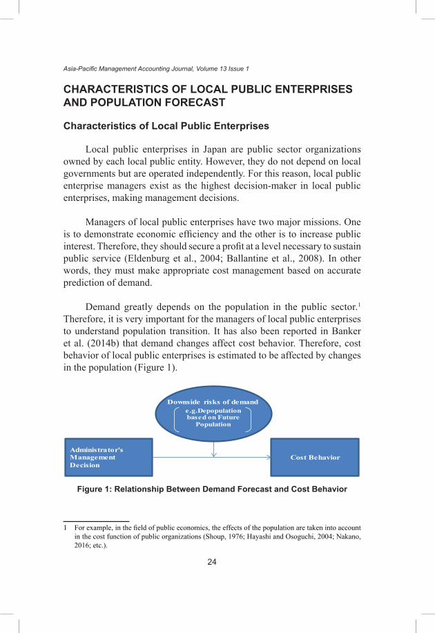
Demand greatly depends on the population in the public sector.1 Therefore, it is very important for the managers of local public enterprises to understand population transition. It has also been reported in Banker et al. (2014b) that demand changes affect cost behavior. Therefore, cost behavior of local public enterprises is estimated to be affected by changes in the population (Figure 1).

e.g.Depopulation based on Future

Population

Administrator's Management Decision

Cost Behavior

Downside risks of demand

Figure 1: Relationship Between Demand Forecast and Cost Behavior

1 For example, in the field of public economics, the effects of the population are taken into account in the cost function of public organizations (Shoup, 1976; Hayashi and Osoguchi, 2004; Nakano, 2016; etc.).

25


And we would like to explain supplementarily about another mission, publicity. Businesses of local public enterprises include social infrastructure businesses such as water supply, industrial water supply, electricity, gas, transportation, and service business such as hospital, nursing care etc. Every business is an indispensable service for residents’ lives. Such public services are subject to government entry restrictions and fee restrictions.2 In other words, the businesses that local public enterprises are responsible for are businesses that require the introduction of large-scale human and material capital such as social infrastructure, or high risk businesses where service supply is not sufficiently done only by the market principle. For this reason, “Market Failure” in Economics exists, and there are many projects for which a commercial business entity finds it difficult to enter. As a result, there are many industries with a high market share in local public enterprises (Table 1).

Table 1: Market Share of Local Public Enterprises

Type of Businesses Market Share (%)

Water Supply 99.5

Industrial Water Supply 99.9

Sewerage 91.3

Transportation *1 13.4

Electric Power 1.1

Gas Power 2.3

Hospital 12.3

Wholesale Market *2 13.1

Car Parking *3 -Source: (excluded Wholesale Market): “The Local Public Enterprises Yearbook No.60(2013)” *1 Average of Railway, Car Transport, Monorail and Shipping, *2 Source: Endo (2013), *3 No data

Trend of Population in Japan and Future Population Estimates

Changes in the population in Japan have two characteristics. One is the population structure where the percentage of elderly people in the population 2 The new entry company cannot do business without obtaining permission. In addition, official price

system such as summary cost method and medical fee are introduced for the fee.

26


is higher than other generations. And the other is that the trend has changed dramatically that the population may decrease after 2006.

In connection with the first feature, though elderly people are over 65 years old, in Japan, in 2005 the proportion of elderly people in the population exceeded 20%, and labelled as a super aging society. For this reason, Japan is said to be one of the world’s highest population with elderly people, and elderly people with health risks have a pension as their main source of income, so their reliance on public services is high.3 It is pointed out in the field of public economics and public finance that the changing population composition by age in this way leads to a change in the demand for public services in the medium and long term (Hayashi and Osoguchi, 2004; nakano, 2016; etc.). Therefore, in order to carry out effective cost management, to accurately grasp the demand forecast and respond to the change is very important. And managers must also pay attention to the change in the proportion of population by age in order to cope with the change in demand. Thus, in order to verify cost behavior of local public enterprises, it is necessary to verify it while paying attention to the trend of a population composition by age.

As the second feature, in Japan, the total population has declined since 2006. In Japan, the population has consistently increased since 1945 after World War, but its trend has changed significantly. And the National Institute of Population and Social Security estimates the population in the future and predicts that the population decline will continue into the future.4 Local public enterprises must rebuild their capacity to the capacity corresponding to the demand drop of population decline and to downsize management resources so as not to generate unnecessary slack. Therefore, a management based on future population estimation is indispensable not only for local public enterprises but also for all public organizations.5 There 3 Medical expenses for the elderly has exceeded 35% of the national medical expenses since 2000

and continues to increase. The nursing care expenditure was 0.7% of GDP in 2000, but it doubled to 1.9% in 2013. In addition, the ratio of elderly person 60 years or older is higher than 50% among welfare recipients.

4 Most recently, estimates are conducted in 1997, 2002, 2006, 2012 and 2017.5 In public works projects carried out by the government, it is explained that proper operation

of population projection in the future is important for demand forecasting (Ministry of Internal Affairs and Communications “Advice based on the findings about demand for public works project predictions” (August, 2008). This material is used as a reference material in formulating future management plans in many public organizations including local public enterprises (Nishioka et al., 2007a; nishioka et al., 2007b).

27


are three estimates for this future population decline prediction: optimistic scenario (high estimate), neutral scenario (middle estimate), pessimistic scenario (low order estimation), but in all scenarios the future population will be in a decreasing trend. And, it is reported by the census that it is after 2006 that the population decline actually started.6

Therefore, from 2006 onwards, the population decrease scenario based on future population estimation will show the downside risk of demand. Banker et al. (2014b) explains that the downside risk of demand is a cause of sticky costs. If the managers misread the demand forecast, it will hold a large amount of unnecessary slack. Conversely, if the capacity is excessively reduced, it will lead to a crisis that the service will be insufficient for demand. In other words, it can be said that managers are in an environment where accurate demand forecasting and cost management must be performed based on population projections in the future.

124,000

125,000

126,000

127,000

128,000

129,000

130,000

1999 2000 2001 2002 2003 2004 2005 2006 2007 2008 2009 2010 2011 2012 2013

1997Medium variant projections 1997High variant projections 1997Low variant projections

2002Medium variant projections 2002High variant projections 2002Low variant projections

populaotionscale:1,000people

Figure 2: Population Projections for Japan (High, Medium and Low Variant Projections)

6 The word “population decline” was used for the first time in “2005 preliminary population report of the 2005 census population” published by the Ministry of Internal Affairs and Communications in December 2005. http://www.stat.go.jp/info/today/009.htm

28


PRIOR STUDIES AND HYPOTHESIS DERIVING

Prior Studies

Empirical studies of cost behavior have been actively studied over the last ten years. It has become clear that cost changes asymmetrically with respect to the change in activity amount (sticky costs and anti-sticky costs). However, there are only a few studies in cost behavior for public sector organizations, and the research contents are limited. In this section, we confirmed prior studies from two points of research on cost behavior of public organizations and the relationship between demand forecast and cost behavior.

Bradbury and Scott (2014) and Cohen et al. (2014) investigate local public entities. And they clarified that there is an asymmetric diversity in cost behavior of the local public entity. They explain that factors that cause sticky costs are mainly service expenses for residents. The resident service expense relates to the core competence of the local public entity, and it becomes an incentive to try to improve resident’s satisfaction rating. For this reason, it has been pointed out that managers are less likely to have the incentive to reduce costs even if the tax revenue decreases (Bradbury and Scott, 2014). In addition, it is explained that sticky costs appear from the reason that cost reduction is difficult because provision of public service is a core competence for public sector organizations (Cohen et al., 2014). On the other hand, Cohen et al. (2014) clarifies that anti- sticky costs appear in internal expenses such as administrative expenses not related to core competencies.

However, tax is used for the proxy index of the activity amount in

their analyses. Tax is not a result of consideration of service but one that is obligatorily collected. For this reason, it is pointed out that tax is not suitable as the proxy index representing the change in the activity amount of the organization (Banker et al., 2016). The local public enterprises that we analyzed are getting usage fee as a service consideration as well as for-profit enterprises, so their points are clear.

Kama and Weiss (2013) and Shust and Weiss (2014) excluded public enterprises from the analysis object for the reasons that the accounting

29


methods were different. However, the local public enterprises in Japan are managed by the same accounting standards and methods as for commercial enterprises. Therefore, their points are cleared and the same research technique as the prior studies can be used.

Holzhacker et al. (2015) analyzed cost behavior of hospitals into three categories, private, public, and non-profit by each ownership, clearly shows that sticky costs appear strongly in local public enterprises. However, since they have examined only the hospital business in public services, they do not grasp cost behavior of public services in other business fields. In this respect, our research covers nine businesses including the hospital business, so we can generalize and verify cost behavior of public sector organizations.

Next, we confirm prior studies on demand forecast and the relationship between cost behavior of local public enterprises. Banker et al. (2014b) explain that in situations where demand uncertainty arises, management maintains management resources to respond to changes in demand to maintain idle capacity. For this reason, they say that if the uncertainty of demand is large, sticky costs will increase to maintain capacity.

On the other hand, when the possibility of demand falling below forecast increases, that is, when the downside risk of demand is high, it is distinguished from uncertainty of demand. And, they explain that sticky costs appear in this case (Banker et al.,2014b). According to Banker et al. (2014b), if the downside risk of demand is high, it will lower the average of demand. Therefore, they are explaining that sticky costs appear because it comes with a lot of needless resources on business to the demand forecast, and the idle capacity increases as a result in high fixed cost structure industries.

Thus, when sticky costs appear, it is divided into the case where demand is uncertain and the case where downside risk of demand arises and they insist that sticky costs appear as a result of each different cost management.

Banker et al. (2014a) clarify that there are differences in the decision-making stance when management is optimistic and when it is pessimistic. That is, if management is optimistic, it is expected that future expectations

30


will be high, so management resources will be kept intact, if it is pessimistic, management resources will be adjusted.

Characteristics of this research not only clarify whether sticky costs are confirmed in the cost behavior of public organizations, but also the relationship between market share and uncertainty of demand forecast, and future demand forecast and the downside risk of demand.

Hypothesis Setting

In previous studies on cost behavior of public organizations, both sticky costs and anti-sticky costs appear, and an asymmetric cost behavior has been confirmed (Bradbury and Scott, 2014; Cohen et al., 2014; Holzhacker et al., 2015; etc.). In addition, Nagasawa and Hosomi (2016) analyzed cost behavior of local public enterprises in Japan during the period 1979 to 1998, and confirmed that asymmetry appears in cost behavior. And, they suggest the possibility that the business environment, the cost structure, the market share, and the pricing procedure influence as a factor of the asymmetric cost behavior.

Focusing on the business environment pointed out by them, in Japan, since 1999, the population which substitutes for demand changed significantly. Concretely, the percentage of elderly people in Japan’s population composition by age until 1998 was low compared to the present. However, as confirmed in the previous section, in 2005, Japan began to enter a super aging society stage and changed to an era where the proportion of elderly people is remarkably in-creasing. Therefore, it can be said that it shifted to a business environment clearly different from the analysis period of Nagasawa and Hosomi (2016) when demand changes are examined from the population structure.

Elderly people are highly dependent on public services, but pension is the center of income, so it is difficult to increase fee income. Bradbury and Scott (2014) and Cohen et al. (2014) pointed out that even though tax revenue declines, residents’ services are the core competence of public organizations and incentives to reduce their expenses do not work, and sticky costs will occur. As the demand for public services has increased due to the increase in elderly people, man-agers have had to reduce the

31


flexibility of cost adjustment. In other words, it can be said that the business environment has undergone a major change due to changes in population composition by age. Therefore, unlike the analysis result of nagasawa and Hosomi (2016), it is thought that sticky costs appear in the cost behavior of local public enterprises. Then,

H1: The sticky costs appear in the cost behavior of local public enterprises.

Next, Nagasawa and Hosomi (2016) pointed out that the market share is one factor that affects cost behavior of local public enterprises. Banker et al. (2014b) pointed out that sticky costs appear when demand uncertainty rises. Conversely, when the uncertainty of demand is low, theoretical and empirical validation has not been done on how cost behavior changes. Theoretically, the uncertainty of demand decreases in a business environment where the market share is high and the future demand forecast is high. Therefore, it is not necessary for managers to hold slacks, and cost adjustment should be done so as to be an optimal management re-source. In this case, the idle capacity cost decreases, and sticky costs become weak or it seems that anti-sticky costs appear. Three businesses of water supply business, industrial water supply business and sewerage business maintain the market share of 90% or more as shown in Table 1. In these three businesses, the market share is high, so it can be said that it is in a business environment in which more accurate demand forecasting can be performed than other businesses. Nagasawa and Hosomi (2016) also revealed that anti-sticky costs appear in the water supply business and the industrial water supply business in the analysis of cost behavior by industry. Then,

H2: In businesses with a high market share, sticky costs are weaker than that of businesses with low monopolization, or anti-sticky costs appear.

Finally, we would like to examine the change in cost behavior from the relationship between the three future population estimation scenarios and the downside risk of demand. Banker et al. (2014b) asserts that sticky costs appear when there is a downside risk of demand, apart from the uncertainty of demand. Three population estimation prospects that represent the demand forecast of local public enterprises are the optimistic scenario, neutral scenario, and pessimistic scenario. However, all of these predicted that the future population will decline. In other words, it can be said that

32


the business environment of Japanese public organizations has a situation in which the downside risk of demand is high. In particular, since 2006, population declines have also been reported in the census. Banker et al. (2014b) analyzed commercial companies, but we think that local public enterprises are different from commercial companies. In other words, we think that local public enterprises can make demand forecasts based on population, and because the demand forecast accuracy is high, managers can respond to the downside risk of demand. Therefore, we think that sticky costs show a weak value or anti-sticky costs show even when the downside risk of demand increases due to the declining population since 2006. Managers of local public enterprises are considered to be capable of cost management based on a long-term management plan without holding large amounts of unnecessary slacks. Then,

H3: Because the downside risk of demand rises after 2006, sticky costs become weak more than before that.

RESEARCH METHOD

Sample Selection and Descriptive Statistics

In this study, we analyzed local public enterprises in Japan since 1999 which Nagasawa and Hosomi (2016) did not analyze. The analysis period is 15 years from 1999 to 2013. The reason for this is to avoid bias due to the change in accounting methods because the accounting method of local public enterprises was changed with the revision of the law in 2014.

Sample data were targeted at 9 industries (water supply business, industrial water supply business, transportation business, electric power business, gas power business, hospital business, sewerage business, wholesale market business, and car parking business) based on the “Local Public Enterprise Yearbook” by the Autonomy Local Finance Bureau of the Ministry of Public Management, Home Affairs, Posts and Telecommunications.

In our analysis model, since the year-on-year ratio was used, except for the 1999 data, the number of samples was 41,194 fiscal year data. From

33


this data, further outliers of 1% above and below were excluded. Eventually the number of samples was 4,342 businesses, and 39,803 data. Descriptive statistics are shown in Table 2. The largest number of samples is 20,363, the water supply business, accounting for 51.16%. The second largest number of samples is hospital business 10,989 data, accounting for 27.61%. And the third largest number of samples is 3,253, sewerage business data, accounting for 8.17%, the fourth largest is 3,080, industrial water business, accounting for 7.74%. In the other projects, the number of samples is less than 5% of the total. The point where the present study is different from nagasawa and Hosomi (2016) is a point that the toll road business is not included in the analysis. Since the toll road business was entrusted or transferred to private enterprises, it was no longer a local public enterprise.

As a feature of the data, the operating expenses, the average value of operating revenues, and the standard deviation are highest in the transportation business. And the minimum value includes 0 yen for operating expenses and operating revenues. This means including preparations for start-up and preparation for disposal. Although some studies exclude these samples, survival bias is generated by excluding these samples, so we decided to include them in this study. And the water supply business is the largest for the maximum value.

And, in this study, these samples were converted in a natural logarithm and used for analysis.

34


Table 2: Descriptive Statistics*Scale: 1,000 yen

Mean Standarddeviation

Minimum Lowerquartile

Median Upperquartile

Maximum numberof firm-

Cost（Operating costs）* 2,612,574 8,799,640 0 221,487 662,522 2,151,206 287,019,811Revenue（Operating revenues）* 2,755,903 10,869,173 0 239,630 671,813 2,144,273 343,940,347ln cost t/cost t-1 0.0024 0.0757 -0.4990 -0.0284 0.0009 0.0303 0.5087ln revenue t/revenue t-1 -0.0006 0.0737 -0.6526 -0.0242 -0.0023 0.0216 0.6419Cost（Operating costs）* 1,548,498 8,312,254 0 185,332 395,952 1,055,683 287,019,811Revenue（Operating revenues）* 1,829,384 9,941,144 0 217,217 463,236 1,217,356 343,940,347ln cost t/cost t-1 0.0053 0.0739 -0.4990 -0.0274 0.0011 0.0320 0.5087ln revenue t/revenue t-1 0.0005 0.0570 -0.5997 -0.0214 -0.0045 0.0141 0.6239Cost（Operating costs）* 439,601 903,945 0 24,339 161,663 427,028 7,998,631Revenue（Operating revenues）* 562,334 1,149,919 0 23,598 172,163 566,361 10,943,486ln cost t/cost t-1 -0.0041 0.1045 -0.4982 -0.0457 -0.0043 0.0375 0.4999ln revenue t/revenue t-1 -0.0016 0.0863 -0.5840 -0.0159 0.0000 0.0109 0.5922Cost（Operating costs）* 4,097,754 16,494,054 0 128,629 477,270 1,894,689 225,035,329Revenue（Operating revenues）* 5,195,664 23,407,597 0 57,751 343,483 57,751 341,558,184ln cost t/cost t-1 0.0146 0.0788 -0.4764 -0.0154 0.0081 -0.0154 0.4929ln revenue t/revenue t-1 0.0234 0.0904 -0.6526 -0.0121 0.0084 -0.0121 0.6419Cost（Operating costs）* 11,283,879 23,086,602 0 616,783 2,099,192 10,968,929 138,555,307Revenue（Operating revenues）* 11,737,793 26,872,233 0 509,212 1,672,011 10,845,291 155,059,483ln cost t/cost t-1 -0.0265 0.0812 -0.4816 -0.0575 -0.0202 0.0102 0.4580ln revenue t/revenue t-1 -0.0262 0.0928 -0.6122 -0.0464 -0.0155 0.0074 0.5557Cost（Operating costs）* 2,222,829 5,213,301 0 300,991 637,249 1,479,712 40,287,262Revenue（Operating revenues）* 2,382,385 5,523,493 0 330,796 691,594 1,531,321 40,270,247ln cost t/cost t-1 0.0107 0.0756 -0.2547 -0.0309 0.0043 -0.0309 0.4891ln revenue t/revenue t-1 0.0099 0.0688 -0.6239 -0.0247 0.0051 -0.0247 0.4456Cost（Operating costs）* 2,177,425 1,585,314 30,139 1,083,237 1,853,304 2,891,793 7,926,889Revenue（Operating revenues）* 2,648,441 1,914,715 45,709 1,291,597 2,225,493 3,540,690 9,506,942ln cost t/cost t-1 -0.0044 0.0711 -0.3572 -0.0422 -0.0102 0.0302 0.3839ln revenue t/revenue t-1 -0.0118 0.0631 -0.3742 -0.0406 -0.0104 0.0107 0.4312Cost（Operating costs）* 4,175,345 4,512,187 0 974,274 2,319,061 5,954,692 31,602,391Revenue（Operating revenues）* 3,772,942 4,265,283 0 812,593 2,022,084 812,593 32,298,365ln cost t/cost t-1 -0.0022 0.0657 -0.4888 -0.0274 0.0012 -0.0274 0.5049ln revenue t/revenue t-1 -0.0068 0.0873 -0.6494 -0.0397 0.0010 -0.0397 0.6249Cost（Operating costs）* 2,267,100 4,212,595 66,223 267,661 602,699 1,839,599 16,928,397Revenue（Operating revenues）* 1,963,711 3,743,950 0 178,288 571,458 1,418,043 14,497,486ln cost t/cost t-1 -0.0148 0.0738 -0.4109 -0.0412 -0.0167 0.0087 0.4347ln revenue t/revenue t-1 -0.0148 0.0394 -0.4207 -0.0266 -0.0111 0.0022 0.0510

Gas Power 422

Hospital 10,989

WholesaleMarket 193

Sewerage 3,253

Transportation 819

ElectricPower 542

IndustrialWater Supply 3,080

Total 39,803

Water Supply 20,363

*Scale: 1,000 yen

Mean Standarddeviation

Minimum Lowerquartile

Median Upperquartile

Maximum numberof firm-

Cost（Operating costs）* 95,731 73,103 2,791 50,318 83,077 120,878 372,239Revenue（Operating revenues）* 135,424 98,231 4,533 73,697 103,079 192,007 499,078ln cost t/cost t-1 -0.0211 0.1155 -0.4468 -0.0703 -0.0219 0.0219 0.4063ln revenue t/revenue t-1 -0.0406 0.1103 -0.5347 -0.0896 -0.0281 0.0141 0.2633

Car Parking 142

Analytical Model

The model from Anderson et al. (2003) has been adopted in many studies as an empirical research method for cost behavior (Banker and Byzalov, 2014; etc.). This model was also used for research targeting public organizations, and the asymmetry of cost has been clarified (Bradbury and Scott, 2014; etc.). And since Nagasawa and Hosomi (2016) also used this model, it is effective in comparison with their analysis results. Therefore, we decided to use the Anderson et al. (2003) model to verify hypothesis 1 and hypothesis 2.

35


Model I


12

Model I

In this formula, Cost represents operating expenses and Revenue represents operating revenue. The Decrease Dummy is a dummy variable that takes 1 if the operating revenue declines compared with the previous year and 0 in other cases.

Ifβ2 is 0, the operating revenue and the operating expenses are in a proportional relationship, but ifβ2 is a negative value it indicates sticky costs, and in the contrary when it becomes a plus, it indicates anti-sticky costs.

In addition, in the verification of hypothesis 3, in order to take into account the influence of the trend of population decline that began in 2006, verification is carried out by Model II which adds the after dummy variable to Model I.

Model II

In this formula, Cost represents operating expenses, Revenue represents operating revenue. Decrease Dummy is a dummy variable that takes 1 if the operating revenue declines compared with the previous year and 0 in other cases. After dummy is a dummy variable in which it assumes after the fiscal year 2006 to be 1.

RESULT

Using Model I, we verified cost behavior of local public enterprises through panel data analysis (Table 3). As a result of the analysis, a significant result was obtained in all of the pooled model, the fixed effect model, and the random effect model. And, as a result of the Hausman test, the fixed effect model represented the most suitable result. β2 showed a negative value of -0.830. From this result, it was confirmed that sticky costs appeared in cost behavior of the local public enterprises from 1999 to 2013. Nagasawa and Hosomi (2016) analyzed cost behavior between 1979 and 1998 and confirmed anti-sticky costs. The result of this analysis contrasts with the analysis result of Nagasawa and Hosomi (2016). We focused on demand in the business environment and thought that the change in the composition ratio of population by age due to the increase in elderly people influences cost behavior, but this hypothesis 1 was supported.

titi

titi

ti

ti

ti

ti

venuevenue

DummyDecreasevenuevenue

CostCost

,1,

,,2

1,

,10

1,

,

ReRe

ln*_*ReRe

ln*ln εβββ +⎥⎥⎦

⎤

⎢⎢⎣

⎡+

⎥⎥⎦

⎤

⎢⎢⎣

⎡+=

⎥⎥⎦

⎤

⎢⎢⎣

⎡

−−−

⎥⎥⎦

⎤

⎢⎢⎣

⎡+

⎥⎥⎦

⎤

⎢⎢⎣

⎡+=⎥

⎦

⎤⎢⎣

⎡

−−− 1,

,,2

1,

,10

1.

,

ReRe

ln*_*ReRe

lnlnti

titi

ti

ti

ti

ti

venuevenue


CostCost

βββ

titi

titi After

venuevenue

DummyDecrease ,1,

,,3 *

ReRe

ln*_* εβ +⎥⎥⎦

⎤

⎢⎢⎣

⎡+

−


If β2 is 0, the operating revenue and the operating expenses are in a proportional relationship, but if β2 is a negative value it indicates sticky costs, and in the contrary when it becomes a plus, it indicates anti-sticky costs.


Model II


12

Model I


Ifβ2 is 0, the operating revenue and the operating expenses are in a proportional relationship, but ifβ2 is a negative value it indicates sticky costs, and in the contrary when it becomes a plus, it indicates anti-sticky costs.


Model II


RESULT

Using Model I, we verified cost behavior of local public enterprises through panel data analysis (Table 3). As a result of the analysis, a significant result was obtained in all of the pooled model, the fixed effect model, and the random effect model. And, as a result of the Hausman test, the fixed effect model represented the most suitable result. β2 showed a negative value of -0.830. From this result, it was confirmed that sticky costs appeared in cost behavior of the local public enterprises from 1999 to 2013. Nagasawa and Hosomi (2016) analyzed cost behavior between 1979 and 1998 and confirmed anti-sticky costs. The result of this analysis contrasts with the analysis result of Nagasawa and Hosomi (2016). We focused on demand in the business environment and thought that the change in the composition ratio of population by age due to the increase in elderly people influences cost behavior, but this hypothesis 1 was supported.

titi

titi

ti

ti

ti

ti

venuevenue


CostCost

,1,

,,2

1,

,10

1,

,

ReRe

ln*_*ReRe

ln*ln εβββ +⎥⎥⎦

⎤

⎢⎢⎣

⎡+

⎥⎥⎦

⎤

⎢⎢⎣

⎡+=

⎥⎥⎦

⎤

⎢⎢⎣

⎡

−−−

⎥⎥⎦

⎤

⎢⎢⎣

⎡+

⎥⎥⎦

⎤

⎢⎢⎣

⎡+=⎥

⎦

⎤⎢⎣

⎡

−−− 1,

,,2

1,

,10

1.

,

ReRe

ln*_*ReRe

lnlnti

titi

ti

ti

ti

ti

venuevenue


CostCost

βββ

titi

titi After

venuevenue

DummyDecrease ,1,

,,3 *

ReRe

ln*_* εβ +⎥⎥⎦

⎤

⎢⎢⎣

⎡+

−


RESULT

Using Model I, we verified cost behavior of local public enterprises through panel data analysis (Table 3). As a result of the analysis, a significant result

36


was obtained in all of the pooled model, the fixed effect model, and the random effect model. And, as a result of the Hausman test, the fixed effect model represented the most suitable result. β2 showed a negative value of -0.830. From this result, it was confirmed that sticky costs appeared in cost behavior of the local public enterprises from 1999 to 2013. nagasawa and Hosomi (2016) analyzed cost behavior between 1979 and 1998 and confirmed anti-sticky costs. The result of this analysis contrasts with the analysis result of Nagasawa and Hosomi (2016). We focused on demand in the business environment and thought that the change in the composition ratio of population by age due to the increase in elderly people influences cost behavior, but this hypothesis 1 was supported.

Table 3: Cost Behavior of Local Public Enterprises

Coefficient Pooled Fixed-effect Random-effect

β0 0.0015 *** 0.0009 ** 0.0015 ***

3.54 2.01 3.51

β1 0.4939 *** 0.4811 *** 0.4939 ***

68.73 57.73 68.11

β2 -0.0568 *** -0.0830 *** 0.0568 ***

-5.07 -6.24 -5.03

Adj.R2 0.2076 0.1930 0.2076

N 39,803 39,803 39,803

DW 2.1763 2.3961 2.1763 H-Test statistic (degree of freedom) P-value

135.15 2 0Upper data indicates coefficient estimates, under data indicates t-statistics *: significant at 10% level, **: significant at 5% level, ***: significant at 1% level Adj.R2=Adjusted R2, N=Number of Observations, DW=Durbin-Watson ratio, H-Test:Hausman Test

Next, we confirm cost behavior from the correlation between market share and demand forecast for hypothesis 2. We compared cost behavior between the three businesses, water supply, industrial water supply, sewerage, which has a market share of more than 90%, and other projects (Table 4). As a result of the analysis, significant results were obtained in all of the pooled model, the fixed effect model, and the random effect model.

37


And, as a result of the Hausman test, the fixed effect model showed the best result. In three businesses with a high market share, β2, indicated sticky costs, at -0.1287, but in the other businesses where the market share was low, β2 was -0.0395. As a result, we assumed that sticky costs weakened or anti-sticky costs occurred due to the low uncertainty of demand when market share was high, but hypothesis 2 was not supported.

For reference, the cost behavior for each industry is shown in Table 5, but a variety of cost behavior was confirmed for each type of industry. This result was partially different from Nagasawa and Hosomi (2016).

38


H

igh

Mar

ket S

hare

Bus

ines

ses†1

Low

Mar

ket S

hare

Bus

ines

ses†2

Coe

ffici

ent

Pool

edFi

xed-

effe

ctR

ando

m-

effe

ctPo

oled

Fixe

d-ef

fect

Ran

dom

-ef

fect

β 00.

0020

**

*0.

0017

**

*0.

0020

**

*-0

.001

0 *

-0.0

011

**-0

.001

0 **

*

3.76

3.

01

3.71

-1

.65

-1.6

7 -1

.65

β 10.

4933

**

*0.

4883

**

*0.

4933

**

*0.

5093

**

*0.

4698

**

*0.

5093

**

*

52.9

6 44

.47

52.2

5 48

.14

40.0

7 48

.22

β 2-0

.110

1 **

*-0

.128

7 **

*-0

.110

1 **

*-0

.047

0 **

*-0

.039

5 **

*-0

.047

0 **

*

-6.6

3 -6

.58

-6.5

4 -3

.18

-2.3

6 -3

.18

Adj

.R2

0.14

53

0.12

18

0.14

53

0.37

47

0.37

69

0.37

47

N26

,696

26,6

9626

,696

13,1

07

13,1

07

13,1

07

DW

2.23

84

2.45

33

2.23

84

1.97

42

2.19

73

1.97

42

H-T

est

stat

istic

(deg

ree

of

freed

om)

P-v

alue

stat

istic

(deg

ree

of

freed

om)

P-v

alue

23.0

8

2

0

158.

95

2

0

Tabl

e 4:

Rel

atio

nshi

p B

etw

een

Mar

ket S

hare

and

Cos

t Beh

avio

r

Upp

er d

ata

indi

cate

s co

effic

ient

est

imat

es, u

nder

dat

a in

dica

tes

t-sta

tistic

s, *

: sig

nific

ant a

t 10%

leve

l, **

: sig

nific

ant a

t 5%

leve

l, **

*: s

igni

fican

t at 1

% le

vel,

Adj

.R2=

Adj

uste

d R

2, N

=Num

ber o

f Obs

erva

tions

, DW

=Dur

bin-

Wat

son

ratio

, H-T

est:

Hau

sman

Tes

t†1

Wat

er S

uppl

y B

usin

ess,

Indu

stria

l Wat

er S

uppl

y B

usin

ess,

Sew

erag

e B

usin

ess,

†2

Oth

er b

usin

esse

s

39


Table 5: Cost Behavior by Industrial Classification (Additional Analysis)

0.0035 *** 0.0033 *** 0.0035 *** -0.0018 -0.0011 -0.0018 0.0012 0.0018 0.00136.20 5.60 6.11 -0.85 -0.49 -0.84 0.74 1.14 0.75

0.6149 *** 0.6074 *** 0.6149 *** 0.2286 *** 0.1951 *** 0.2286 *** 0.3823 *** 0.3600 *** 0.3795 ***

54.92 50.45 54.14 7.03 5.38 6.94 20.15 17.15 19.82-0.0881 *** -0.1013 *** -0.0881 *** 0.0772 0.1122 ** 0.0772 -0.2998 *** -0.2897 *** -0.2991 ***

-4.25 -4.47 -4.19 1.58 2.07 1.56 20.15 -7.47 -8.25

H-test

-0.0114 *** -0.0127 *** -0.0114 *** -0.0005 0.0007 -0.0005 -0.0051 * -0.0049 -0.0051-3.95 -4.24 -3.95 -0.12 0.16 -0.12 -1.65 -1.53 -1.63

0.4039 *** 0.3698 *** 0.4039 *** 0.3594 *** 0.3059 *** 0.3594 *** 0.9068 *** 0.8862 *** 0.9068 ***

7.98 6.70 7.97 4.47 3.55 4.41 17.83 16.19 17.620.1130 * 0.1012 0.1130 * -0.0162 0.0567 -0.0162 -0.3932 *** -0.3929 *** -0.3932 ***

1.73 1.40 1.73 -0.12 0.40 -0.12 -4.32 -4.06 -4.27

H-test

0.0002 -0.0001 0.0002 -0.0043 -0.0043 -0.0043 -0.0210 -0.0271 ** -0.02100.36 -0.21 0.36 -0.69 -0.66 -0.68 -1.61 -2.02 -1.61

0.4955 *** 0.4860 *** 0.4955 *** 0.6816 0.5575 0.6816 0.4572 ** 0.5655 ** 0.4572 **

46.25 42.36 46.05 1.31 0.98 1.29 2.01 2.37 2.02-0.0321 ** -0.0416 ** -0.0321 ** 0.0423 0.1385 0.0423 -0.3095 -0.4858 -0.3095

-2.14 -2.56 -2.13 0.07 0.22 0.07 -1.10 -1.63 -1.10

H-test

upper data indicates coefficient estimates, under data indicates t-statistics, *: significant at 10％ level, **: significant at 5％ level, ***: significant at 1％ level,Adj.R2=Adjusted R2, n=number of Observations, DW=Durbin-Watson ratio, H-Test:Hausman Test

0.0246

Electric Power

β0

β1

β2

Adj.R2

Water Supply Industrial Water Supply

Transportation

Pooled Fixed Random Pooled Fixed Random

0.0489n 20,363 3,080

0.0489

β0

β1

β2

Adj.R2 0.2026 0.1795 0.2026

Pooled

DW 2.3075 2.4155 2.3075

Pooled Fixed Random

0.16

0.3014

2.1852

2.0576 2.2031 2.0576

32.65 (2) 0.00 5.28 (2) 0.07

0.3007 0.3014 0.0934 0.0699819

Fixed Random

2.1852 2.3178

193

Pooled Fixed

3.66 (2)

n

9.37 (2) 0.01

RandomHospital Wholesale Market

Fixed

2.1726 2.06603.16 (2)

0.4756

β0

β1

β2

0.21

0.1172

0.1383Adj.R2 0.4119 0.4068 0.4119 0.1383 0.1072

422 542DW 2.4645 2.5845 2.4645 2.0660

0.0934 0.4756 0.4631

Random Pooled

Sewerage

54.28 (2) 0.00

Pooled Fixed Random

10,989

1.82 (2) 0.402.2141

3,2530.1209 0.1383

Car Parking

n

3.79 (2) 0.15DW 2.0449 2.1847 2.0449 2.2141 2.3004

Pooled Fixed Random

2.0900 2.2476142

9.03 (2) 0.01

2.0900

2.0809 2.2927 2.1160

0.0441 0.04120.0412

Gas PowerPooled Fixed Random

Finally, in order to verify hypothesis 3, we performed a panel data analysis using Model II (Table 6). As a result of the analysis, significant results were obtained in all three analysis models. And, as a result of the Hausman test, we found that the fixed effect model is most suitable. The β3 representing cost behavior since 2006 has a negative value of -0.2094. In other words, it is confirmed that sticky costs tended to strengthen after 2006, when the downside risk of demand increased. As a result, hypothesis 3 was not supported.

40


Table 6: Relationship Between Downside Risk of Demand and Cost Behavior

β0 0.0016 *** 0.0013 *** 0.0016 ***

3.98 2.87 3.94

β1 0.4926 *** 0.4775 *** 0.4926 ***

68.74 57.42 68.10

β2 0.0648 *** 0.0525 *** 0.0648 ***

4.73 3.20 4.69

β3 -0.2016 *** -0.2094 *** -0.2016 ***

-15.35 -13.97 -15.21

Adj.R2 0.2122 0.1974 0.2122n 39,803 39,803 39,803

DW 2.1771 2.3961 2.1771statistic (degree of freedom) P-value

117.08 3 0upper data indicates coefficient estimates, under data indicates t-statistics*: significant at 10％ level, **: significant at 5％ level, ***: significant at 1％ level

Adj.R2=Adjusted R2, n=number of Observations, DW=Durbin-Watson ratio, H-Test:Hausman Test

coefficient

H-Test

Including After year 2006 Dummy Variables

Pooled Fixed-effect Random-effect

CONCLUSION

In this research, in order to clarify cost behavior in public organization, we confirm that cost behavior for the local public enterprises owned by local public entities. Together with the work of Nagasawa and Hosomi (2016) covering 1979 to 1998, the analysis period lasts 35 years. Over the long term, we have verified cost behavior of local public enterprises. Based on this point, we will describe the features of this research, the limits of this research and future subjects below.

As the first feature, it can be pointed out that sticky costs are confirmed in the cost behavior of local public enterprise as a whole. This result contrasted with Nagasawa and Hosomi (2016) which confirmed anti-sticky costs. As an external environmental factor affecting asymmetric cost behavior, the impact of the increase in elderly people can be considered. In other words, changes in population composition by age may have influenced cost behavior in local public enterprises. Japan has entered a super aging society in 2005 and pressure is increasing to expand public services for

41


public organizations. Therefore, as for local public enterprise managers, the situation that it was difficult to reduce cost to income decrease continued to cope with the stagnation of the income rate. We thought that changes in the business environment due to the proportion of these population by age group contributed to the asymmetry of cost behavior. However, in this research we cannot fully control these external environmental factors. In future research, it can be said that it is necessary to verify these factors more strictly. In addition, not only external environmental factors, but also analysis of factors within the organization is required.

The second feature is that the influence on cost behavior is confirmed from the interaction of market share and demand forecast. When the market share is high, precise demand forecasting is possible and the uncertainty of demand decreases. For this reason, we thought that the local public enterprise managers did not need to keep track of management resources in preparation for uncertainty of demand, and that sticky costs would decline. However, as a result of the analysis, our conclusion showed the opposite fact. In other words, sticky costs appeared stronger in all of the three businesses of water supply, industrial water supply, and sewerage, which have a high market share, compared to other businesses. This means that even if the reliability of demand due to market share increases, cost behavior of local public enterprises is affected by other factors. In future research, explanation from other factors other than market share rate is required. nagasawa and Hosomi (2016) suggests that pricing and cost structure may influence as other factors affecting cost behavior. Even these factors need to be verified in future research. Furthermore, as additional analysis, we confirmed cost behavior by industry, but the result was different from nagasawa and Hosomi (2016). Therefore, it can be said that a more detailed analysis is necessary for each industry. We would like to identify the factors that change cost behavior for each industry type in future research.

Finally, as the third feature, this study focused on the downside risk of demand. Public services are mainly conducted by local public enterprises, so we used the population as a proxy variable for demand. Then, we confirmed how local public enterprises are performing cost management for three scenarios of a future population forecast (optimism, neutral, pessimism). As a result of the analysis, after 2006 when the downside risk of demand by the population decline rose, it became clear that sticky costs strengthen. This

42


suggests that local public enterprises may be affected more than anticipated by the cost structure specific to the public organization, i.e. high fixed costs, low variable costs. And this indicates that the mechanism of sticky costs found in private enterprises was confirmed in public organizations in the event of downside risks as argued by Banker et al. (2014b). In other words, it means that the administrators of local public enterprises could not adjust their management resources in preparation for the downside risk of demand like private enterprises managers caused by their high fixed cost structure.

The costs behaviors of public organizations are expected to be elucidated not only from academics but also at the practical level and further exploration is required in the future.

REFERENCES

Anderson, M. C., Banker, R. D. & Janakiraman, S. (2003). Are selling, general, and administrative costs “sticky”?. Journal of Accounting Research, 41(1), 47-63.

Ballantine, J., Forker, J. & Greenwood, M. J. (2008). The governance of CEO incentives in English nHS hospital trusts. Financial Accountability and Management, 24(4), 385-410.

Banker, R. D. & Byzalov, D. (2014). Asymmetric Cost Behavior. Journal of Management Accounting Research, 26(2), 43-79.

Banker, R. D., Byzalov, D., Ciftci, M. & Mashruwala, R. (2014a). The moderating effect of prior sales changes on asymmetric cost behavior. Journal of Management Accounting Research, 26(2), 221–242.

Banker, R. D., Byzalov, D. & Plehn-Dujowich, J. M. (2014b). Demand uncertainty and cost behavior. The Accounting Review, 89(3), 839–865.

Banker, R. D., Byzalov, D., Fang, S. & Liang, Y. (2016). Cost behavior research. Working Paper, Social Science Research network.

Bradbury, M. E. & Scott, T. (2014). Do managers understand asymmetric cost behavior?, Working Paper, Social Science Research network.

43


Calleja, K., Steliaros, M. & Thomas, D. C. (2006). A note on cost stickiness: Some international comparisons. Management Accounting Research, 17(2), 127-140.

Cohen, S., Karatzimas, S. & Naoum, V. C. (2014). The sticky cost phenomenon at the local government level: Empirical evidence from Greece. Working Paper, Social Science Research network.

Eldenburg, L., Hermalin, B. E., Weisbach M. S. & Wosinska, M. (2004). Governance, performance objectives and organizational form: Evidence from hospitals. Journal of Corporate Finance, 10(4), 527-548.

Endo, S. (2013). Local public enterprises current situation and issues-with the focus on water supply business. The Japan Economic Research Institute monthly report, 423, 44-53.

Hayashi, Y., & Osoguchi, K. (2004). Supply of local public services and productivity analysis. Kwansei Gakuin University Departmental Bulletin Paper, 58(2), 1-28.

Holzhacker, M., Krishnan, R. & Mahlendorf, M. D. (2015). The impact of changes in regulation on cost behavior. Contemporary Accounting Research, 32(2), 534-566.

Kama, I. & Weiss, D. (2013). Do earnings targets and managerial incentives affect sticky costs?. Journal of Accounting Research, 51(1), 201-224.

Ministry of Internal Affairs and Communications Local Public Finance Bureau Editing. (2001-2015). Local Public Enterprise Yearbook Part47-61, Institute of Local Finance.

Nagasawa, S. & Hosomi, S. (2016). Empirical Study on Asymmetric Cost Behavior of the Public Sector Organizations-Analysis of the Sticky Costs of Local Public Enterprises, Proceedings of APMAA 2016, no.69.

Nakano, K. (2016). Effects of population and household structures on residential electricity demand – A literature review and future research agenda. The Electric Power Economic Research, 63, 35-49.

44


Nishioka, H., Yamauchi, M. & Koike, S. (2007a). Implementation status of future estimates of population and households in local governments, usage situation and correspondence to population-related measures - In the case of Municipalities. Journal of Population Problems, 63(2), 57-66.

Nishioka, H., Yamauchi, M. & Koike, S. (2007b). Implementation status of future estimates of population and households in local governments, usage situation and correspondence to population-related measures - In the case of Municipalities. Journal of Population Problems, 63(4), 56-73.

Shoup, C. S. (1976). Collective Consumption and Relative Size of the Government Sector. Public and Urban Economics, 191-212.

Shust, E. & Weiss, D. (2014). asymmetric cost behavior-sticky costs expenses versus cash flows. Journal of Management Accounting Research, 26(2), 81-90.

Subramaniam, C. & Weidenmier, M. L. (2003). Additional evidence on the sticky behavior of costs. Working Paper, Texas Christian University.

Weiss, D. (2010). Cost behavior and analysts’ earnings forecasts. The Accounting Review, 85, 1441-1474.

study on downside risk of demand and cost behavior …

Documents