study on the cost and contribution of the rail...
TRANSCRIPT

Prepared by Steer Davies Gleave
Study on the Cost and Contribution of the Rail Sector
European Commission
Directorate General for Mobility
and Transport
Final Report
September 2015
Our ref: 22783801
Client ref: MOVE/B2/2014-761


The information and views set out in this report are those of the author(s) and do not necessarily reflect
the official opinion of the Commission. The Commission does not guarantee the accuracy of the data
included in this study. Neither the Commission nor any person acting on the Commission’s behalf may
be held responsible for the use which may be made of the information contained therein.
Steer Davies Gleave has prepared this material for European Commission Directorate General for
Mobility and Transport. This material may only be used within the context and scope for which Steer
Davies Gleave has prepared it and may not be relied upon in part or whole by any third party or be used
for any other purpose. Any person choosing to use any part of this material without the express and
written permission of Steer Davies Gleave shall be deemed to confirm their agreement to indemnify
Steer Davies Gleave for all loss or damage resulting therefrom. Steer Davies Gleave has prepared this
material using professional practices and procedures using information available to it at the time and as
such any new information could alter the validity of the results and conclusions made.
Study on the Cost and Contribution of the Rail Sector
European Commission
Directorate General for Mobility
and Transport
Final Report
September 2015
Our ref: 22783801
Client ref: MOVE/B2/2014-761
.
Prepared by:
Prepared for:
Steer Davies Gleave
28-32 Upper Ground
London SE1 9PD
European Commission Directorate
General for Mobility and Transport
Rue de Mot 28
B-1040 Brussels
Belgium
+44 20 7910 5000
www.steerdaviesgleave.com

Study on the Cost and Contribution of the Rail Sector | Final Report
September 2015 | i
Contents
1 Introduction ....................................................................................................................... 1
Background ................................................................................................................................... 1
Study objectives and methodology .............................................................................................. 2
Organisation of this report ........................................................................................................... 4
2 Data collection ................................................................................................................... 5
Overview ....................................................................................................................................... 5
Data collection .............................................................................................................................. 7
Addressing data limitations and gaps ......................................................................................... 10
Summary of rail industry characteristics and trends .................................................................. 11
3 Key performance indicators .............................................................................................. 26
Overview ..................................................................................................................................... 26
Selection of KPIs.......................................................................................................................... 26
KPI analysis ................................................................................................................................. 29
Conclusions ................................................................................................................................. 41
4 Clustering analysis ............................................................................................................ 42
Overview ..................................................................................................................................... 42
Clustering principles ................................................................................................................... 42
Clustering methodology ............................................................................................................. 44
5 Efficiency gap analysis ...................................................................................................... 55
Data Envelopment Analysis ........................................................................................................ 55
Conclusions ................................................................................................................................. 62
6 Scenario assessment ......................................................................................................... 63
Scenario definition ...................................................................................................................... 63
Estimating economic impacts ..................................................................................................... 67
Core scenario .............................................................................................................................. 72
Supplementary scenario analysis ............................................................................................... 75
7 Policy implications ............................................................................................................ 80
The current policy context .......................................................................................................... 80
The need for industry restructuring ........................................................................................... 81

Study on the Cost and Contribution of the Rail Sector | Final Report
September 2015 | ii
Potential policy development ..................................................................................................... 83
Recommendations for further work ........................................................................................... 85
Figures
Figure 1.1: The analytical framework ........................................................................................... 4
Figure 2.1: Trends in input indicators (2007 = 100) .................................................................... 12
Figure 2.2: Trends in output indicators (2007 = 100) ................................................................. 13
Figure 2.3: Trends in financial indicators (2007 = 100, adjusted for HICP) ................................ 15
Figure 2.4: Cost and contribution of the EU rail sector (2012) ................................................... 17
Figure 2.5: Fare revenue per passenger kilometre (2012) ......................................................... 18
Figure 2.6: Freight revenue per tonne kilometre (2012) ............................................................ 19
Figure 2.7: Operating costs per train kilometre by Member State (2012) ................................. 20
Figure 2.8: Passenger and freight activity (2012) ....................................................................... 21
Figure 2.9: Train km per inhabitant (2012) ................................................................................. 22
Figure 2.10: Passenger km per inhabitant (2012) ...................................................................... 23
Figure 2.11: Freight tonne kilometres per unit GDP (2012) ....................................................... 23
Figure 2.12: Change in Passenger Rail Mode Share (2003 to 2012) ........................................... 24
Figure 2.13: Change in Rail Freight Mode Share (2003 to 2012) ................................................ 25
Figure 3.1: Change in Track Utilisation (2007 to 2012) – train kilometres per track kilometre . 30
Figure 3.2: Change in Passenger Train Utilisation (2007 to 2012) – passenger kilometres per
passenger train kilometre ........................................................................................................... 31
Figure 3.3: Change in Freight Train Utilisation (2007 to 2012) – freight tonne kilometres per
freight train kilometre ................................................................................................................ 32
Figure 3.4: Track utilisation and population density (2012) – logarithmic scale ........................ 34
Figure 3.5: Track utilisation and passenger train utilisation (2012) – logarithmic scale ............ 35
Figure 3.6: Track utilisation and freight train utilisation (2012) – logarithmic scale .................. 36
Figure 3.7: Passenger track utilisation and freight track utilisation (2012) – logarithmic scale . 37
Figure 3.8: Passenger track utilisation and freight track utilisation (2012) – absolute figures .. 38
Figure 3.9: Cost efficiency and passenger km (2012) – logarithmic scale .................................. 39
Figure 3.10: Subsidy and revenue (2012) – logarithmic scale .................................................... 40
Figure 4.1: Illustration of clustering analysis (2012) ................................................................... 45
Figure 4.2: Dendrogram and nested cluster examples ............................................................... 47

Study on the Cost and Contribution of the Rail Sector | Final Report
September 2015 | iii
Figure 4.3: Relative size of clusters by GDP, population, passenger km and freight tonne km
(2012) .......................................................................................................................................... 51
Figure 4.4: GDP per capita by Member State and cluster (2012) ............................................... 52
Figure 4.5: Rail network length by Member State and cluster (2012) ....................................... 52
Figure 4.6: Passenger train utilisation versus total track utilisation by Member State and cluster
(2012) .......................................................................................................................................... 53
Figure 4.7: Freight train utilisation versus total track utilisation by Member State and cluster
(2012) .......................................................................................................................................... 54
Figure 5.1: Indicative efficiency frontier for railway operations ................................................ 56
Figure 5.2: Total capital productivity technical efficiency scores (DEA model 1 VRS) - 2012 (not
re-based) ..................................................................................................................................... 58
Figure 5.3: Technical efficiency scores for passenger rail (DEA model 3 VRS) – 2012 (not re-
based) ......................................................................................................................................... 59
Figure 5.4: Technical efficiency scores for rail freight (DEA model 4 VRS) – 2012 (not re-based)
.................................................................................................................................................... 60
Figure 5.5: Track utilisation technical efficiency scores (DEA model 5 VRS) – 2012 (not re-
based) ......................................................................................................................................... 61
Figure 5.6: Train utilisation technical efficiency scores (DEA model 6 VRS) – 2012 (not re-based)
.................................................................................................................................................... 62
Figure 6.1: Rail sector output multipliers for a sample of Member States ................................ 70
Figure 6.2: Rail sector employment multipliers for a sample of Member States ....................... 71
Figure 6.3: NPV of GVA impacts 2015-2030 (core scenario) ...................................................... 73
Figure 6.4: Estimate of employment impacts 2015-2030 (core scenario) ................................. 73
Figure 6.5: NPV of external benefits 2015-2030 (core scenario) ............................................... 74
Figure 6.6: Comparison of outputs (rail passenger km) between the core scenario and
supplementary scenario analysis in 2030 ................................................................................... 78
Figure 6.7: Comparison of outputs (rail tonne km) between the core scenario and
supplementary scenario analysis in 2030 ................................................................................... 78
Figure 7.1: The EU policy framework for the rail sector ............................................................. 80
Tables
Table 2.1: Summary of study data ................................................................................................ 5
Table 2.2: Contextual and Infrastructure Data ............................................................................. 7
Table 2.3: Harmonisation Data ..................................................................................................... 8
Table 2.4: Input and Output Data ................................................................................................. 8
Table 2.5: Financial and Staffing Data Sources ............................................................................. 9

Study on the Cost and Contribution of the Rail Sector | Final Report
September 2015 | iv
Table 3.1: Key performance indicators for rail systems and their main issues .......................... 27
Table 3.2: Review of the inputs and outputs used in previous studies ...................................... 28
Table 3.3: Change in secondary KPIs (2007 – 2012) ................................................................... 33
Table 4.1: Literature review – key determinants of utilisation and efficiency of rail ................. 43
Table 4.2: Clustering variables .................................................................................................... 44
Table 4.3: Summary of clustering analysis ................................................................................. 47
Table 4.4: Clustering outputs (passenger) – test 4 ..................................................................... 48
Table 4.5: Clustering outputs (freight) – test 8 ........................................................................... 49
Table 4.6: Final clusters .............................................................................................................. 50
Table 5.1: Selected data envelopment analysis models ............................................................. 57
Table 6.1: Using clusters to re-base DEA outputs ...................................................................... 64
Table 6.2: The core scenario efficiency gaps and potential operating cost savings .................. 65
Table 6.3: Rail sector output and employment multipliers (indirect) for a sample of Member
States .......................................................................................................................................... 69
Table 6.4: Summary of scenario results and impacts (2010 prices, 2010 PV) ............................ 74
Table 6.5: Road Price Cross Elasticities of Demand for Rail by Member State .......................... 76
Table 6.6: Comparison between the supplementary scenario analysis and the core scenario by
cluster ......................................................................................................................................... 79

Study on the Cost and Contribution of the Rail Sector | Final Report
September 2015 | v
Appendices
A Data collection – Member State notes
B Data tables
C Clustering methods
D Clustering outputs
E Data envelopment analysis models
F Scenario modelling tool – record of assumptions
G Bibliography

Study on the Cost and Contribution of the Rail Sector | Final Report
September 2015 | 1
1 Introduction Background
1.1 The rail sector makes a substantial contribution to the European Union (EU) economy, directly
employing 577,000 people across passenger and freight operations and the provision of track
and station infrastructure1. Some estimates suggest that, once the entire supply chain for rail
services is taken into account (e.g. including train manufacturing, catering services etc.), the
economic footprint of the rail sector in Europe extends to 2.3 million employees and €143
billion of Gross Value Added (some 1.1% of the total)2. It is also critical to the EU strategy for
improving economic and social cohesion and connectivity within and between Member States,
including through the further development of the TEN-T rail corridors, and is expected to play
a major role in the reduction of carbon and other emissions from transport. The development
of the sector has been encouraged over a period of more than 20 years through the
implementation of an extensive legislative framework, including three major packages of
legislation, and a fourth package currently being considered by the European Council and
Parliament.
1.2 Accordingly, the 2011 White Paper, Roadmap to a Single European Transport Area – Towards a
competitive and resource efficient transport system, envisages much greater use of rail
transport in the future. More specifically, the White Paper includes a number of rail-related
objectives supporting a more efficient and sustainable transport system for the EU, in
particular:
30% of road freight over 300km shifting to other modes by 2030, and 50% by 2050;
Completion of the European high speed rail network by 2050, and maintaining a dense rail
network in all Member States;
By 2050 the majority of medium-distance passenger transport should go by rail;
A fully functional TEN-T core network by 2030, with a high quality/capacity network by
2050;
Connection of all core network airports to the rail network (ideally the high speed
network) by 2050;
Deployment of the European Rail Traffic Management System (ERTMS);
The establishment of the framework for a European multimodal information,
management and payment system by 2020; and
Full application of user pays/polluter pays principles in transport.
1 EU Transport in Figures: Statistical Pocketbook 2015 (European Commission)
2 The Economic Footprint of Railway Transport in Europe (CER, 2014)

Study on the Cost and Contribution of the Rail Sector | Final Report
September 2015 | 2
1.3 However, while the rail sector has achieved significant volume growth in recent years, rail’s
modal share remains below expectations, accounting for only 6.6% of passenger km and 10.8%
of tonne-km within the EU28 in 20123. These average shares reflect a wide range of
experience in different Member States, but are generally considered symptomatic of an
overall lack of competitiveness driven by insufficient investment and inadequate customer-
focused innovation across the EU (notwithstanding that the sector also absorbs at least €36
billion of public funds annually, some €80 for every European citizen)4.
1.4 As a result of these and other factors, rail has failed to challenge the dominance of road in
both freight and passenger transport and, despite the considerable growth of high speed
networks, has been unable to arrest the small but steady increase in the share of short to
medium distance passenger transport taken by aviation since the mid-1990s. Moreover,
ongoing constraints on the availability of public funds following the financial crisis are
expected to reduce the traditional resources available for rail investment in a number of
Member States.
1.5 Therefore it is opportune to look in depth at how different national rail systems have
performed over recent years, and to learn from the best how to improve the efficiency of
railways.
Study objectives and methodology
Study objectives
1.6 Against this background, the primary objectives of this study are to:
provide a 'broad brush' analysis of the trends in overall performance of different national
rail systems; and
conduct a scenario analysis assessing the potential societal benefits of a better performing
rail sector.
1.7 In meeting these objectives, the study encompasses:
An analysis of recent trends in passenger and freight volumes as well as associated fare
levels and revenues;
A review of operating and capital expenditure, recognising that this may be incurred by
train operators, infrastructure managers and other parties, and of the related flow of
funding between rail sector stakeholders;
Estimation of the contribution of the sector according to a range of economic, social and
sustainability metrics including GVA, employment and emissions; and
An analysis of sector efficiency, based on measures of asset utilisation and indicators of
financial performance.
Overview of methodology
1.8 The methodology developed to meet the study objectives is broadly sequential, although
there is, necessarily, some iteration required between analytical steps described below.
3 EU Transport in Figures: Statistical Pocketbook 2015 (European Commission) – includes non-surface
modes
4 Fourth Report on Monitoring Development of the Rail Market (European Commission, 2014)
Study on the Cost and Contribution of the Rail Sector | Final Report
September 2015 | 3
1.9 The first step was to collect and harmonise data for all Member States that have a rail network
(i.e. excluding Malta and Cyprus). This included demographic and economic data, indicators of
rail sector resources and the value added by rail. This data was then used to generate primary
and secondary Key Performance Indicators (KPIs), which measure the performance of an
economic entity (in this case Member State railways) and allow comparability over time as
well as against other entities. KPIs are typically ratios of key outputs to inputs, but can also be
measures of service quality derived, for example, from customer surveys. Our approach to
selecting and finalising KPIs for this study was based on the following criteria:
Adherence to policy goals (do the KPIs match the policy levers available to the
Commission to improve performance?);
Literature review (which input and output measures have been successfully identified and
analysed in past studies?); and
Data availability (obtaining good quality, comparable data on railway operations across
the whole of the European Union is challenging).
1.10 We then analysed relationships between primary and secondary KPIs, and a range of
exogenous variables in order to inform the subsequent clustering exercise. This step is
intended to control for the variation in the performance of Member State rail systems that
could be attributed to exogenous factors. Clustering analysis is conducive to achieving two
objectives: first, to establish a basic categorisation of national rail systems for the purpose of
the current analysis and to inform future benchmarking exercises at the EU level; and
secondly, to increase the discriminatory power of the efficiency analysis which follows by
reducing the heterogeneity of the sample.
1.11 A technique called data envelopment analysis (DEA) was then used to measure the technical
efficiency gap between rail systems. Given a set of inputs (e.g. rail sector employees, track-
km) and outputs (e.g. passenger-km, train-km), DEA fits an efficiency frontier which envelops
the data. In specifying the DEA analysis, the choice of inputs and outputs was determined to
match the capital efficiency measures established in the analysis of KPIs.
1.12 Finally, both the outputs of the clustering exercise and the DEA were used to define the scope
of achievable efficiency improvements. Further assumptions were required regarding the
timescales over which these improvements can be made and the mechanisms through which
they can be achieved (informed by consideration of secondary KPIs and additional indicators).
Supplementary data sources and analyses were then used to quantify the impact of efficiency
improvements over time, on a range of economic and social indicators.
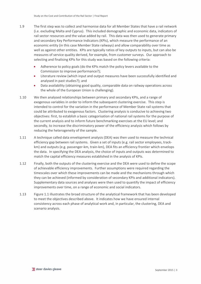
1.13 Figure 1.1 illustrates the broad structure of the analytical framework that has been developed
to meet the objectives described above. It indicates how we have ensured internal
consistency across each phase of analytical work and, in particular, the clustering, DEA and
scenario analysis.

Study on the Cost and Contribution of the Rail Sector | Final Report
September 2015 | 4
Figure 1.1: The analytical framework
Organisation of this report
1.14 This remainder of this report is organised according to the following structure, which aligns
with the methodology described above:
Chapter 2: Data collection and harmonisation
Chapter 3: Development of Key Performance Indicators
Chapter 4: Clustering analysis
Chapter 5: Measuring the efficiency gap
Chapter 6: Scenario assessment
Chapter 7: Policy implications.

Study on the Cost and Contribution of the Rail Sector | Final Report
September 2015 | 5
2 Data collection Overview
2.1 In order to understand the nature and performance of railways across Member States, we
undertook an extensive data collection and harmonisation exercise. As summarised in Table
2.1, we have collected data sets for 32 indicators across 26 Member States.
Table 2.1: Summary of study data
Contextual and infrastructure data Harmonisation data Rail sector data
Area Currencies (average) Freight rolling stock
Border countries Currencies (year-end) Passenger rolling stock
Urban population Market share Employees
Ports linked by rail Operating costs
TEN corridors Public subsidies
Cost of congestion Passenger revenue
Rail Satisfaction Freight revenue
Population Train kilometres
GDP per capita Rail passenger kilometres
Registered cars Rail tonne kilometres
Motorways Rail mode share
Total passenger kilometres
Total tonne kilometres
Road fatalities
Rail fatalities
In-use rail network track kilometres
High speed rail network kilometres
Electrified rail network kilometres
2.2 This chapter provides an overview of the data collection process, and provides commentary
regarding the quality of data collected. It describes the following stages of the data collection,
collation and review process:
Contextual and infrastructure data: the sources of the demographic, economic and
infrastructure data used to understand the context in which each Member State’s rail
network operates.
Harmonisation data: the data used to ensure comparability between Member States,
and the approach to making comparisons where the data was incomplete (as in the case
of rail market share).

Study on the Cost and Contribution of the Rail Sector | Final Report
September 2015 | 6
Input and output data: the data collected to understand the resources used by, and the
outputs from, each rail system. The inputs are expressed in terms of rolling stock,
employees, operational costs and subsidy, with outputs measured in terms of revenues,
passenger kilometres, tonne kilometres and mode share.
Data limitations and gaps: issues encountered in seeking to collect a complete data set
(covering all indicators across all Member States and years) and the actions taken to
address these as far as possible.
Country specific issues: the key data-related issues that are particular to each Member
State, and the actions taken to address these.
Quality assurance: the measures we have taken to ensure that the data set is as robust
as possible given the scope of, and timescales for, the study.
Rail industry characteristics and trends: presentation of trends in key input and output
indicators over time.
2.3 We have obtained data for the period 2003 to 2013 wherever possible. For a number of
reasons, however, we have focussed our subsequent analysis on the period 2007 to 2012. In
particular:
Member States were only captured within the dataset from the year of their accession to
the European Union. Since 11 Member States considered in this study joined after 2004,
it is not possible to draw meaningful comparisons before this point.
Where it exists, data from primary sources prior to 2007 is increasingly difficult to access
and interpret through time.
Non-statutory third-party datasets (such as that provided by the International Union of
Railways), while often being the only consistently available source, suffer from coverage
and self-selection bias.
Data release schedules mean that comprehensive data for 2013 has been difficult to
obtain.
2.4 For some indicators, such as “Country Area”, we have only collected data for one year, since
we would not expect any material changes in the value of the indicator over a 10-year period.
For a small number of data series (for example, total passenger kilometres and mode share) it
has been necessary to use secondary data sources to calculate indicators for some Member
States.
2.5 In line with the study requirements we have attempted to capture at least 90% of all activity
across freight and passenger railway undertakings and infrastructure providers.

Study on the Cost and Contribution of the Rail Sector | Final Report
September 2015 | 7
Data collection
Contextual and infrastructure data
2.6 A summary of the contextual and infrastructure related data that we have collected for this
study is provided in Table 2.2.
Table 2.2: Contextual and Infrastructure Data
Data Unit Date(s) Source Comment
CONTEXTUAL DATA
Area Km2 2013 CIA Factbook
It has been assumed this data has not changed significantly between 2003-14
Border countries Number 2013 CIA Factbook
Urban population % 2013 Eurostat
Ports linked by rail Number 2013 EU TENtec
TEN corridors Number 2013 EU TENtec
Cost of congestion €m 2010 PRIMES model Data limited to 2010
Rail Satisfaction % satisfied 2012 Eurobarometer Data limited to 2012
Population Million people 2003-13 EU Statistical Pocketbook
GDP per capita € 2006-13 Eurostat In real terms
Registered cars Thousand cars 2003-12 EU Statistical Pocketbook
Motorways Length in km 2003-11 EU Statistical Pocketbook
Definitions of “motorway” vary by Member State
Total passenger kilometres
Billion passenger km
2003-12 EU Statistical Pocketbook
Sum of passenger km for car, bus, coach, tram and rail
Total tonne kilometres
Billion tonne km 2003-12 EU Statistical Pocketbook
Sum of road, rail and inland waterway tonne km
Road fatalities Fatalities 2003-12 EU Statistical Pocketbook
Rail fatalities Fatalities 2003-12 EU Statistical Pocketbook
INFRASTRUCTURE DATA
In-use rail network (line length)
Length in km 2003-12 EU Statistical Pocketbook
High speed rail network
Length in km 2003-13 EU Statistical Pocketbook
High speed is defined as >250 km per hour
Electrified rail network
Length in km 2007-12 EU Statistical Pocketbook
2.7 We are satisfied that the data summarised in Table 2.2 is sufficiently consistent and complete
for the purposes of this study. There are a small number of apparent anomalies in some data
sets. For example, the Italian High Speed Rail network appears to have reduced in size
between 2006 and 2007. However, we do not believe that these inconsistencies will have any
material impact on the study.
Study on the Cost and Contribution of the Rail Sector | Final Report
September 2015 | 8
Harmonisation data
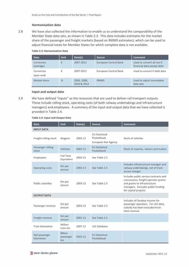
2.8 We have also collected the information to enable us to understand the comparability of the
Member State data sets, as shown in Table 2.3. This data includes estimates for the market
share of the passenger and freight markets (based on RMMS estimates), which can be used to
adjust financial totals for Member States for which complete data is not available.
Table 2.3: Harmonisation Data
Data Unit Date(s) Source Comment
Currencies (average)
€ 2007-2012 European Central Bank Used to convert all non € financial data except debt
Currencies
(year-end)
€ 2007-2012 European Central Bank Used to convert € debt data
Market share % 2006, 2008, 2010 & 2012
RMMS Used to adjust incomplete data sets
Input and output data
2.9 We have defined “inputs” as the resources that are used to deliver rail transport outputs.
These include rolling stock, operating costs (of both railway undertakings and infrastructure
managers) and employees. A summary of the input and output data that we have collected is
provided in Table 2.4.
Table 2.4: Input and Output Data
Data Unit Date(s) Source Comment
INPUT DATA
Freight rolling stock Wagons 2003-12
EU Statistical Pocketbook
European Rail Agency
Stock of vehicles
Passenger rolling stock
Vehicles 2003-12 EU Statistical Pocketbook
Stock of coaches, railcars and trailers
Employees Full Time Equivalent
2003-13 See Table 2.5
Operating costs €m per annum
2003-13 See Table 2.5 Includes infrastructure manager and railway undertakings, net of track access charges
Public subsidies €m per annum
2003-13 See Table 2.5
Includes public service contracts and concessions, freight operator grants and grants to infrastructure managers. Excludes public funding for capital projects
OUTPUT DATA
Passenger revenue €m per annum
2003-13 See Table 2.5
Includes all farebox income for passenger operators. For UIC data, subsidy has been excluded from total revenue
Freight revenue €m per annum
2003-13 See Table 2.5
Train kilometres Million train km
2007-12 UIC Database
Rail passenger kilometres
Billion passenger km
2003-12 EU Statistical Pocketbook

Study on the Cost and Contribution of the Rail Sector | Final Report
September 2015 | 9
Rail tonne kilometres
Billion tonne km
2003-12 EU Statistical Pocketbook
Rail mode share (split into freight and passenger)
% 2003-12
EU Statistical Pocketbook and calculations by SDG (which align)
Ratio of rail passenger or tonne kilometres to total passenger or tonne kilometres (across all modes)
2.10 Very little financial and staffing data was available from the sources listed in Table 2.4. In
order to fill these gaps, we commissioned a group of country experts to investigate each
Member State. In most cases, this involved studying the Annual Reports and Accounts for the
largest Infrastructure Managers and Operators in each country. A summary of the data
sources used to complete the country data sets is provided in Table 2.5.
Table 2.5: Financial and Staffing Data Sources
MS Source Source Type Year(s) Revenue Costs Staffing Debt
AT OBB Annual Reports 2003-12
BE Infrabel Regulatory Accounts 2003-13
BE SNCB Regulatory Accounts 2003-13
BG DB Schenker Company Website 2013
BG UIC Database 2007-12
CZ UIC Database 2007-12
DE DB AG Annual Reports 2003-13
DK DB Schenker Company Website 2013 DK Banedanmark Regulatory Accounts 2003-13
DK DSB Regulatory Accounts 2003-13
EE UIC Database 2009-12
EL OSE Regulatory Accounts 2006-13
EL TrainOSE Regulatory Accounts 2006-13
EL UIC Database 2007-13
ES ADIF Regulatory Accounts 2003-13
ES DB Schenker Company Website 2013 ES RENFE Regulatory Accounts 2003-13
FI UIC Database 2007-12
FI RMMS Survey Data 2013 FR DB Schenker Company Website 2013
FR RFF Regulatory Accounts 2003-13
FR SNCF Regulatory Accounts 2003-13
HU DB Schenker Company Website 2014 HU UIC Database 2007-12
IE Iarnród Éireann Regulatory Accounts 2003-13
IT DB Schenker Company Website 2014 IT Arrigo, Di Foggia Academic Paper 2003-13
IT Corte dei Conti Publication 2003-12
IT Eurofound Statistical bulletin 2005
IT FS Group Regulatory Accounts 2003-12
IT NTV Regulatory Accounts 2011-12
IT UIC Database 2003-12
IT Wikipedia Article 2007-08
LT UIC Database 2009-12
LU CFR Annual Report 2007-12
LV UIC Database 2009-12
NL DB Schenker Company Website 2014 NL NS Regulatory Accounts 2003-13
NL Prorail Regulatory Accounts 2003-13
PL DB Schenker Company Website 2013
PL UIC Database 2007-12
PT CP Regulatory Accounts 2003-13

Study on the Cost and Contribution of the Rail Sector | Final Report
September 2015 | 10
MS Source Source Type Year(s) Revenue Costs Staffing Debt
PT REFER Regulatory Accounts 2003-13
RO DB Schenker Company Website 2013
RO UIC Database 2007-12
SE Banverkets Regulatory Accounts 2004-09
SE RMMS Survey Data 2009-12
SE UIC Database 2007-12
SK UIC Database 2007-12
UK BRES Labour statistics 2003-13
UK DB Schenker Company Website 2013 UK DRDNI Regulatory accounts 2003-13
UK Network Rail Regulatory accounts 2003-13
UK ORR Data portal reports 2003-13
UK Uni. Leeds Academic paper 2007-09
Addressing data limitations and gaps
Summary of key limitations and gaps
2.11 While the process outlined above enabled us to fill in a number of gaps, we were not able to
compile a complete data set for all Member States. The principal outstanding gaps and
limitations are summarised below.
Not all private sector operators (particularly freight operators) report at a Member State
level. In part, this is because many transport operators prefer to present their regulatory
accounts as consolidated accounts, which often combine modes and/or markets. We
were able to obtain a very small amount of country specific data from some operators (for
example, DB Schenker for the year 2013). However, this data is insufficient to allow an
analysis of trends over time. In order to address this issue, we used RMMS data to
estimate the proportion of the market captured by the data collected. We then inflated
incomplete totals (notably for revenues and operating costs) on the basis of the
associated estimates of missing values. This issue relates only to operators and not to
infrastructure managers.
Employee data usually does not include employees who work for sub-contractors or
agencies. Additionally, some organisations report their staffing data on a Full Time
Equivalent (FTE) basis, while others simply report the number of employees. The absence
of supply chain and, in most cases, smaller operator data from our database leads us to
believe that the total employment figures represent an underestimate. We have been
able to cross-reference some Member State data with other published data. For example,
our UK estimate for 2013 is within 5% of the Rail Delivery Group’s estimate for direct
employment in the rail industry in the same year (although their estimate for indirect
employment is much higher).
The public subsidy stated in each operator’s regulatory accounts may not include indirect
public subsidy, such as that provided through capital programmes or tax relief. The
definition of subsidy is not always clear in some Annual Reports and Accounts. Where
possible, we have included Public Service Contracts and Concessions – although these
funding streams are not always obvious. Additionally, not all public funding intended for
capital investment is explicitly separated from the subsidy intended to help operators
meet their day-to-day costs. While we have taken a number of steps to exclude funding
intended for capital investment projects from our data, it is possible that some costs
related to capital expenditure have been captured in the dataset.
Net debt data is not widely reported by the UIC or in regulated accounts, and it has
therefore not been possible to provide aggregate debt figures for several Member States.
Study on the Cost and Contribution of the Rail Sector | Final Report
September 2015 | 11
In spite of these constraints, we have estimated debt for some of the largest
Infrastructure Managers in the EU, in particular those in Germany, France, the UK and
Italy. However, we do not believe that debt data is sufficiently robust or comparable to
use in this study.
We have tried as far as possible to be consistent in the interpretation of operating
expenditure (net of track access charges), which for the purposes of this study includes
depreciation, amortisation, maintenance, renewals and finance costs for both railway
undertakings and infrastructure managers5. However, not all Annual Reports and
Accounts disaggregate their operating expenditure in this manner. It is therefore possible
that some capital expenditure (e.g. for enhancements) may have been included in the
operating costs of some organisations.
In many cases it has been difficult to obtain complete data for the years prior to 2007 and
after 2012. We have therefore limited most of our analysis to the years 2007 to 2012
(inclusive).
Quality assurance
2.12 Notwithstanding the issues and limitations of the datasets collected (see Appendix A for
further details for each Member State), we have taken a number of steps to give assurance
that the data collected provides a reasonable representation of the rail operations in each
Member State. Checks have included:
Comparing data provided in published annual accounts data with the UIC database;
Comparing academic studies with other data sources including government statistics and
the UIC database;
Examining trends in each indicator to identify anomalous or outlying data points;
Generating and reviewing the relationship between datasets to ensure that they
demonstrate a reasonable spread and consistency through time and across Member
States;
Supplementing data obtained from desk research with other information provided by
Member State experts, who bring local and sector knowledge and experience; and
Where multiple datasets report the same observations, selecting a preferred value or
series based on the completeness and consistency of the datasets themselves.
2.13 However, notwithstanding these checks, we have not been able to verify the accuracy of the
individual datasets used to inform this study. By focussing on the most recent data in the
subsequent tasks, we have sought to ensure that our analysis is based upon the most accurate
data available.
Summary of rail industry characteristics and trends
2.14 The data collection exercise has enabled us to examine trends in the rail industry at a Member
State and EU level. A summary of high-level trends at an EU-wide level is provided below, with
the underlying data for each Member State reported in Appendix B.
5 Adjustments to avoid the double-counting of track access charges have been applied.

Study on the Cost and Contribution of the Rail Sector | Final Report
September 2015 | 12
Input indicators
Figure 2.1: Trends in input indicators (2007 = 100)
2.15 Rolling stock fleet sizes (vehicles) for both passenger and freight appear to have been in
decline since 2009. This may be due to changes to the characteristics of rolling stock such as
increasing seat densities and larger freight wagons, or economic effects such as asset disposal
or stabling during the economic crisis. Without detailed investigation at a national level, it is
not reasonable to draw any firm conclusions regarding the drivers of these trends, since many
of the observed changes through time may be driven naturally by the rolling stock fleet
replacement cycle rather than any particular policy or commercial imperative.
2.16 At a national level, we note that only 7 out of 26 Member States (Bulgaria, Germany, Latvia,
Luxembourg, Netherlands, Portugal and Romania) have increased the size of their freight
fleets over the five year period, with typical reductions elsewhere of 5% – 15%. In the
passenger market there is a more even split in the number of Member States increasing or
decreasing their fleet sizes but, with the exception of Bulgaria, the railway systems that are
expanding are exclusively higher-income Western European nations.
80
90
100
110
2007 2008 2009 2010 2011 2012
Freight rolling stock Passenger rolling stock Employees
80
90
100
110
2007 2008 2009 2010 2011 2012
Freight rolling stock Passenger rolling stock Employees
Study on the Cost and Contribution of the Rail Sector | Final Report
September 2015 | 13
2.17 There has also been a marked decrease in employment in the rail sector. However, this trend
could be attributed to structural changes in the industry (particularly outsourcing). The
practice of outsourcing is of particular importance when considering absolute levels of
performance whereby, through reducing the number of individuals directly employed by a
railway undertaking or infrastructure manager, the output per employee is perceived to
increase.
2.18 When considering relative performance (i.e. between Member States) it is more important to
understand the prevalence of outsourcing in each country. In this sense, we would expect the
level of outsourcing to vary, primarily, according to network size. In particular, we would
expect larger, more divisible rail networks to have a greater proportion of outsourcing,
thereby over-stating their efficiency relative to smaller Member States. National data suggests
that some Member States may have outsourced activities during the period 2007-2012 (for
example Bulgaria, Czech Republic, Estonia and Greece), although it is not possible to separate
out this effect from general reductions in staff numbers observed across the EU rail sector
over this period.
Output indicators
Figure 2.2: Trends in output indicators (2007 = 100)
80
90
100
110
2007 2008 2009 2010 2011 2012
Train kilometres Rail passenger kilometres Rail tonne kilometres

Study on the Cost and Contribution of the Rail Sector | Final Report
September 2015 | 14
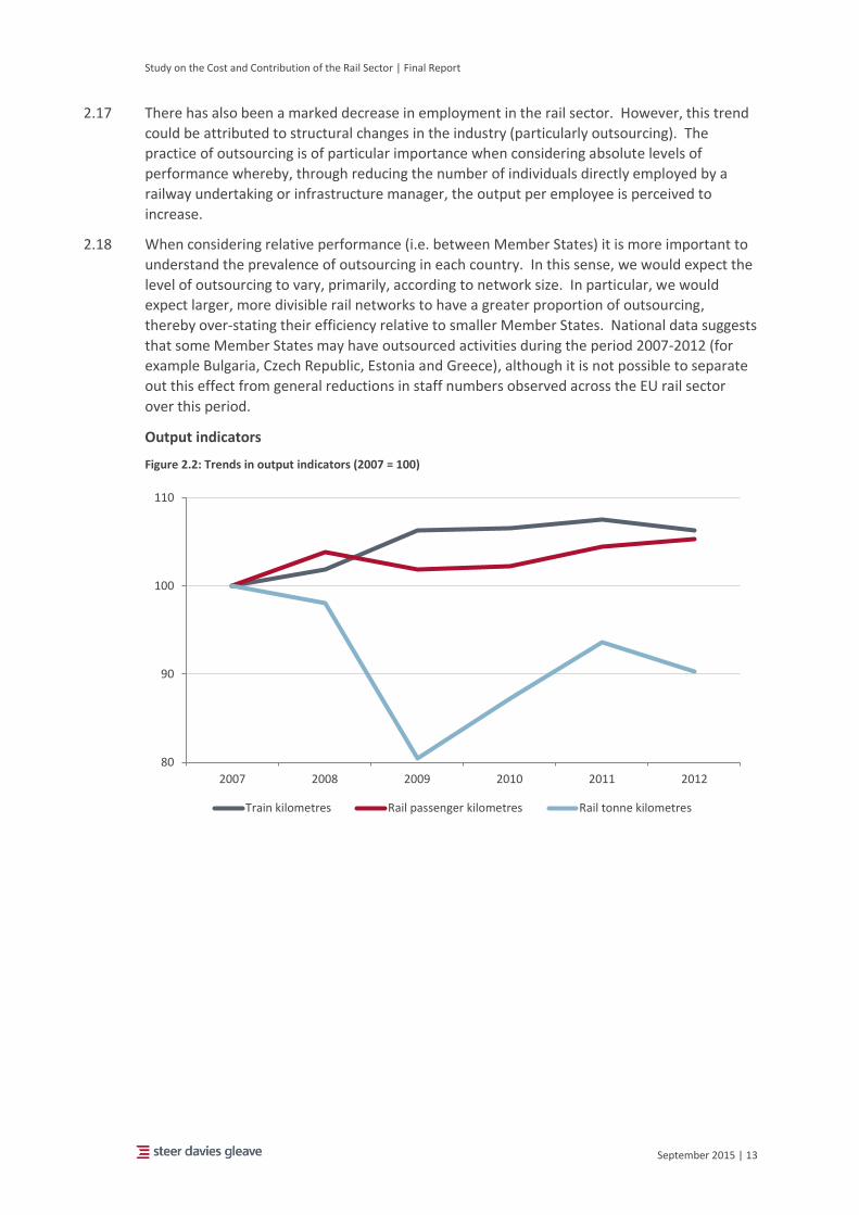
2.19 Despite an unfavourable economic climate across much of the EU over this period, rail
passenger outputs have grown. Figure 2.2 shows that both passenger kilometres and train
kilometres (which include both passenger and freight train movements) have increased by
approximately 1% each year. This is in contrast to the change in rail freight outputs (tonne
kilometres), which have declined by 10% overall in the five years to 2012 despite recovering
substantially since the depth of the recession in 2009.
2.20 The most significant increases in train kilometres have been observed in Western Europe, with
six Member States (Denmark, Germany, Luxembourg, Netherlands, Sweden, UK) expanding
their rail operations by more than 15% between 2007 and 2012. In many cases this is a
consequence of major infrastructure enhancements coming into use during the period, such
as the HSL-Zuid line in the Netherlands (2009), and the West Coast Main Line upgrade works in
the UK (2008). While the majority of other Member States have seen relatively minor changes
in train kilometres since 2007, three countries (Bulgaria, Estonia and Greece) have seen a
significant downturn in activity. Train kilometres in Bulgaria have fallen by 24%, largely
because of the consolidation activity required by its Railway Reform Programme. In Greece,
however, the 38% reduction in train kilometres can be attributed to the reduction in state
funding required as part of the wider fiscal austerity packages implemented from 2010.
2.21 While there have been modest increases in rail passenger kilometres across the EU, this hides
significant variation at a Member State level. In line with trends in train kilometres, the best
performing countries are typically higher income Western European Member States, with the
UK reporting the largest increase in passenger usage of 21%. Slovakia (13%) and the Czech
Republic (5%) are notable exceptions. Alongside Greece (-57%), three Member States
(Croatia, Latvia and Romania) observed reductions in patronage of more than 25%.
In contrast to the passenger railway, freight outputs almost universally declined across Europe
between 2007 and 2012. Only three Member States reported any increase in rail freight
activity, with Denmark (27%) and Latvia (19%) considerably ahead of the UK (< 1%). Some of
the increase in Latvia (3.6 billion tonne kilometres) may be freight traffic that has been
displaced from neighbouring Estonia, which observed a decline in freight volumes of 39% (or
3.3 billion freight kilometres).
80
90
100
110
2007 2008 2009 2010 2011 2012
Train kilometres Rail passenger kilometres Rail tonne kilometres

Study on the Cost and Contribution of the Rail Sector | Final Report
September 2015 | 15
This displacement of freight activity between Baltic States is, in part, due to lower access
charges (both track access charges and port fees) for transit flows in Latvia coupled with the
delivery of increased port capacity6. It may also reflect the political impact of the so called
“scandal of the bronze soldier” when, in 2007, Russia completely stopped its coal and oil
transit via the ports in Estonia. Meanwhile, Latvia managed to attract a considerable amount
of these cargos to its transit corridor.
Financial indicators
Figure 2.3: Trends in financial indicators (2007 = 100, adjusted for HICP)
6 Cargo volumes handled at Latvian ports increased by 23% between 2004 and 2012 (see Rijkure. A and
Sare. I (2013), The Role of Latvian Ports Within Baltic Sea Region, European Integration Studies, 2013 No 7)
80
90
100
110
120
130
140
2007 2008 2009 2010 2011 2012
Passenger revenue Operating costs Subsidies
Study on the Cost and Contribution of the Rail Sector | Final Report
September 2015 | 16
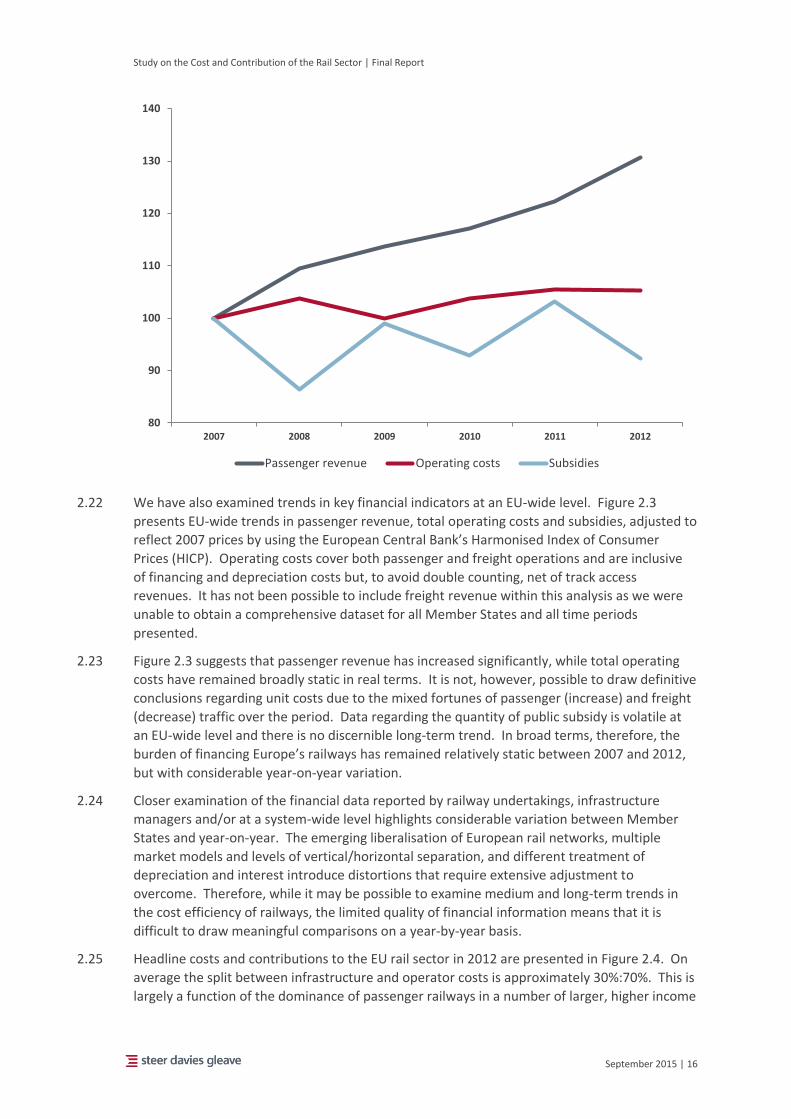
2.22 We have also examined trends in key financial indicators at an EU-wide level. Figure 2.3
presents EU-wide trends in passenger revenue, total operating costs and subsidies, adjusted to
reflect 2007 prices by using the European Central Bank’s Harmonised Index of Consumer
Prices (HICP). Operating costs cover both passenger and freight operations and are inclusive
of financing and depreciation costs but, to avoid double counting, net of track access
revenues. It has not been possible to include freight revenue within this analysis as we were
unable to obtain a comprehensive dataset for all Member States and all time periods
presented.
2.23 Figure 2.3 suggests that passenger revenue has increased significantly, while total operating
costs have remained broadly static in real terms. It is not, however, possible to draw definitive
conclusions regarding unit costs due to the mixed fortunes of passenger (increase) and freight
(decrease) traffic over the period. Data regarding the quantity of public subsidy is volatile at
an EU-wide level and there is no discernible long-term trend. In broad terms, therefore, the
burden of financing Europe’s railways has remained relatively static between 2007 and 2012,
but with considerable year-on-year variation.
2.24 Closer examination of the financial data reported by railway undertakings, infrastructure
managers and/or at a system-wide level highlights considerable variation between Member
States and year-on-year. The emerging liberalisation of European rail networks, multiple
market models and levels of vertical/horizontal separation, and different treatment of
depreciation and interest introduce distortions that require extensive adjustment to
overcome. Therefore, while it may be possible to examine medium and long-term trends in
the cost efficiency of railways, the limited quality of financial information means that it is
difficult to draw meaningful comparisons on a year-by-year basis.
2.25 Headline costs and contributions to the EU rail sector in 2012 are presented in Figure 2.4. On
average the split between infrastructure and operator costs is approximately 30%:70%. This is
largely a function of the dominance of passenger railways in a number of larger, higher income
80
90
100
110
120
130
140
2007 2008 2009 2010 2011 2012
Passenger revenue Operating costs Subsidies

Study on the Cost and Contribution of the Rail Sector | Final Report
September 2015 | 17
Member States. In those countries where freight traffic plays a more significant role, the
proportion of total costs borne by the infrastructure manager is greater.
2.26 On the income side of the equation, roughly 60% of observed costs are covered by fare-box
and freight revenue (40% passenger and 20% freight) and a further 30% by subsidy7. The
remaining 10% (or roughly €10.7bn) is a residual balancing item that is likely to include freight
income not captured at the Member State level (data was not available for all Member States)
and other sources of income such as property rents and retail revenue.
Figure 2.4: Cost and contribution of the EU rail sector (2012)
Source: SDG analysis
2.27 Figure 2.5 highlights the disparity in the average fare revenue per passenger kilometre
between Member States. Of course, average fares hide considerable variation between the
various routes, operators and ticket-types available within Member States. They may also
reflect the typically heavy regulation of rail fares by national governments, with passengers
often paying a fixed fare per kilometre (“kilometric fare”) for standard class travel and a fixed
multiplier for first class travel. Pure kilometric pricing is increasingly rare, but distance-based
fares are still common in a number of Member States. For instance, in the Netherlands the
introduction of the OV-chipcard has been accompanied by a return to kilometric prices,
although these are modulated by region and class of travel and subject to discounts. Trenitalia
in Italy continues to apply kilometric pricing to most regional services operated under Public
Service Contracts.
7 It should be noted that, in some Member States, there may be unobserved or ‘hidden’ cost items, such
as maintenance backlogs, that are not captured in this analysis.
75,724
36,404
46,420
20,011
35,014
10,682
-
20,000
40,000
60,000
80,000
100,000
120,000
Costs Income
€m
illio
n (
20
10
pri
ces)
Operator costs IM costs Passenger revenue Freight revenue Subsidy Other
Study on the Cost and Contribution of the Rail Sector | Final Report
September 2015 | 18
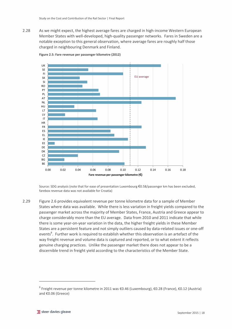
2.28 As we might expect, the highest average fares are charged in high-income Western European
Member States with well-developed, high-quality passenger networks. Fares in Sweden are a
notable exception to this general observation, where average fares are roughly half those
charged in neighbouring Denmark and Finland.
Figure 2.5: Fare revenue per passenger kilometre (2012)
Source: SDG analysis (note that for ease of presentation Luxembourg €0.58/passenger km has been excluded, farebox revenue data was not available for Croatia)
2.29 Figure 2.6 provides equivalent revenue per tonne kilometre data for a sample of Member
States where data was available. While there is less variation in freight yields compared to the
passenger market across the majority of Member States, France, Austria and Greece appear to
charge considerably more than the EU average. Data from 2010 and 2011 indicate that while
there is some year-on-year variation in the data, the higher freight yields in these Member
States are a persistent feature and not simply outliers caused by data-related issues or one-off
events8. Further work is required to establish whether this observation is an artefact of the
way freight revenue and volume data is captured and reported, or to what extent it reflects
genuine charging practices. Unlike the passenger market there does not appear to be a
discernible trend in freight yield according to the characteristics of the Member State.
8 Freight revenue per tonne kilometre in 2011 was €0.46 (Luxembourg), €0.28 (France), €0.12 (Austria)
and €0.06 (Greece)
0.00 0.02 0.04 0.06 0.08 0.10 0.12 0.14 0.16 0.18
BE
BG
CZ
DK
DE
EE
IE
EL
ES
FR
HR
IT
LV
LT
HU
NL
AT
PL
PT
RO
SI
SK
FI
SE
UK
Fare revenue per passenger kilometre (€)
EU average

Study on the Cost and Contribution of the Rail Sector | Final Report
September 2015 | 19
Figure 2.6: Freight revenue per tonne kilometre (2012)
Source: SDG analysis (note that for ease of presentation Luxembourg €0.52/tonne km has been excluded, it was not possible to obtain sufficiently comprehensive freight revenue data for United Kingdom, Sweden, Netherlands, Croatia and Denmark)
2.30 Finally, Figure 2.7 describes total operating costs per train kilometre by Member State. While
there are a few notable outliers (in particular Greece and Croatia), the spread of operating
costs lies broadly in the range of €20 - €40 per train kilometre. Towards the upper end of this
range lie high-income Western European Member States including Belgium, the Netherlands
and Austria with France and Luxembourg higher still. A number of Central European member
States lie towards the lower end of the range including the Czech Republic, Hungary and
Poland.
0.00 0.05 0.10 0.15 0.20 0.25 0.30 0.35
BE
BG
CZ
DK
DE
EE
IE
EL
ES
FR
HR
IT
LV
LT
HU
NL
AT
PL
PT
RO
SI
SK
FI
SE
UK
Freight revenue per tonne kilometre (€)
EU average

Study on the Cost and Contribution of the Rail Sector | Final Report
September 2015 | 20
Figure 2.7: Operating costs per train kilometre by Member State (2012)
0
20
40
60
80
100
120
BE BG CZ DK DE EE IE EL ES FR HR IT LV LT LU HU NL AT PL PT RO SI SK FI SE UK
€ p
er
train
kil
om
etr
e
Railway undertaking(s) Infrastructure manager(s)
EU average

Study on the Cost and Contribution of the Rail Sector | Final Report
September 2015 | 21
Rail market characteristics by Member State
2.31 Figure 2.8 provides high-level statistics regarding the absolute scale of the market for rail by
Member State, as measured by passenger kilometres and freight tonne kilometres. There is
considerable variation in both the size and distribution of rail activity between Member States.
Given the scale of divergence, it will be important to ensure that scale effects are captured
within this study. It is highly likely that the scale of a Member State and its rail network will
have some bearing on the efficiency of delivering rail outputs.
Figure 2.8: Passenger and freight activity (2012)
Source: SDG analysis
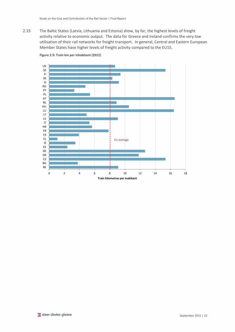
2.32 Figure 2.9, Figure 2.10 and Figure 2.11 use population size and economic output to normalise
rail outputs and permit comparison of rail markets on a more consistent basis. Unsurprisingly,
due to the dominance of passenger rail in a number of Member States, there is a remarkably
close relationship between train kilometres per inhabitant and passenger kilometres per
inhabitant. The top three Member States (excluding Luxembourg) as measured by train
kilometres per inhabitant are Austria, Czech Republic and Sweden9. These share similar
geographic characteristics, in particular the location of all their major cities along the same rail
corridor.
9 Per capita measures for Luxembourg are often skewed due to the significant difference between
workplace and residential populations as a consequence of commuting from neighbouring countries. While we might expect the workplace population to affect rail usage, population statistics are recorded on a residential basis.
0
20
40
60
80
100
120
BE BG CZ DK DE EE IE EL ES FR HR IT LV LT LU HU NL AT PL PT RO SI SK FI SE UK
bill
ion
s
Passenger km Freight tonne km
Study on the Cost and Contribution of the Rail Sector | Final Report
September 2015 | 22
2.33 The Baltic States (Latvia, Lithuania and Estonia) show, by far, the highest levels of freight
activity relative to economic output. The data for Greece and Ireland confirms the very low
utilisation of their rail networks for freight transport. In general, Central and Eastern European
Member States have higher levels of freight activity compared to the EU15.
Figure 2.9: Train km per inhabitant (2012)
0 2 4 6 8 10 12 14 16 18
BE
BG
CZ
DK
DE
EE
IE
EL
ES
FR
HR
IT
LV
LT
LU
HU
NL
AT
PL
PT
RO
SI
SK
FI
SE
UK
Train kilometres per inabitant
EU average

Study on the Cost and Contribution of the Rail Sector | Final Report
September 2015 | 23
Figure 2.10: Passenger km per inhabitant (2012)
Figure 2.11: Freight tonne kilometres per unit GDP (2012)
Source: SDG analysis
- 200 400 600 800 1,000 1,200 1,400 1,600
BE
BG
CZ
DK
DE
EE
IE
EL
ES
FR
HR
IT
LV
LT
LU
HU
NL
AT
PL
PT
RO
SI
SK
FI
SE
UK
Passenger kilometres per inabitant
0 0.2 0.4 0.6 0.8 1 1.2 1.4 1.6 1.8
BE
BG
CZDKDE
EE
IEELES
FR
HRIT
LV
LT
LUHUNL
AT
PLPTRO
SISK
FISE
UK
Freight tonne kilometres per unit GDP (€ )
EU average
EU average
Study on the Cost and Contribution of the Rail Sector | Final Report
September 2015 | 24
Rail mode share
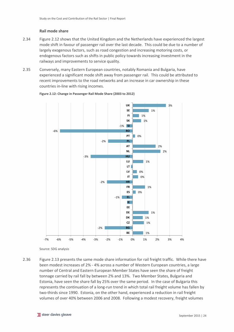
2.34 Figure 2.12 shows that the United Kingdom and the Netherlands have experienced the largest
mode shift in favour of passenger rail over the last decade. This could be due to a number of
largely exogenous factors, such as road congestion and increasing motoring costs, or
endogenous factors such as shifts in public policy towards increasing investment in the
railways and improvements to service quality.
2.35 Conversely, many Eastern European countries, notably Romania and Bulgaria, have
experienced a significant mode shift away from passenger rail. This could be attributed to
recent improvements to the road networks and an increase in car ownership in these
countries in-line with rising incomes.
Figure 2.12: Change in Passenger Rail Mode Share (2003 to 2012)
Source: SDG analysis
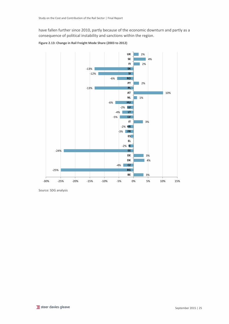
2.36 Figure 2.13 presents the same mode share information for rail freight traffic. While there have
been modest increases of 2% - 4% across a number of Western European countries, a large
number of Central and Eastern European Member States have seen the share of freight
tonnage carried by rail fall by between 2% and 13%. Two Member States, Bulgaria and
Estonia, have seen the share fall by 25% over the same period. In the case of Bulgaria this
represents the continuation of a long-run trend in which total rail freight volume has fallen by
two-thirds since 1990. Estonia, on the other hand, experienced a reduction in rail freight
volumes of over 40% between 2006 and 2008. Following a modest recovery, freight volumes
1%
-2%
1%
1%
1%
-1%
0%
1%
-2%
0%
0%
1%
-3%
2%
2%
-2%
0%
-6%
-1%
1%
1%
1%
3%
-7% -6% -5% -4% -3% -2% -1% 0% 1% 2% 3% 4%
BE
BG
CZ
DK
DE
EE
IE
EL
ES
FR
HR
IT
LV
LT
LU
HU
NL
AT
PL
PT
RO
SI
SK
FI
SE
UK
Study on the Cost and Contribution of the Rail Sector | Final Report
September 2015 | 25
have fallen further since 2010, partly because of the economic downturn and partly as a
consequence of political instability and sanctions within the region.
Figure 2.13: Change in Rail Freight Mode Share (2003 to 2012)
Source: SDG analysis
3%
-25%
-4%
4%
3%
-24%
-2%
-3%
-2%
3%
-5%
-4%
-2%
-6%
1%
10%
-13%
2%
-6%
-12%
-13%
2%
4%
2%
-30% -25% -20% -15% -10% -5% 0% 5% 10% 15%
BE
BG
CZ
DK
DE
EE
IE
EL
ES
FR
HR
IT
LV
LT
LU
HU
NL
AT
PL
PT
RO
SI
SK
FI
SE
UK
Study on the Cost and Contribution of the Rail Sector | Final Report
September 2015 | 26
3 Key performance indicators Overview
3.1 This chapter describes the development and treatment of Key Performance Indicators (KPIs).
These are used to measure the relative efficiency of rail systems and to draw comparisons
between the performance of individual Member States. KPIs can be defined as a set of
quantifiable measures that an industry uses to gauge or compare performance in terms of
meeting their strategic and operational goals.
3.2 The choice of KPIs will vary between industries, depending on their priorities or performance
criteria. They will also be affected by a range of exogenous factors that are outside the direct
control of the industry in question and its agents. Therefore, for this study, we have defined
the following:
Primary KPIs: direct measures of rail sector efficiency such as passenger kilometres per
train kilometre;
Secondary KPIs: potential indicators of efficiency that are within the control of the rail
industry, for example train kilometres per employee; and
Additional indicators: a combination of exogenous measures (e.g. population density) and
endogenous measures (e.g. passenger satisfaction) which may also indirectly affect rail
sector efficiency, largely from a demand-side perspective.
3.3 Primary indicators are the main focus for this study since they describe the relative
performance of rail systems according to efficiency measures over which the Commission has
relatively more influence (e.g. through rolling stock and infrastructure standards, ERTMS,
funding and policy on market access). Secondary indicators provide additional information
about the characteristics and performance of rail systems. Any policy prescription identified
through consideration of secondary KPIs may, however, be beyond the direct control of the
Commission. Other exogenous factors that affect rail sector efficiency but which are largely
outside of the control of both the Commission and individual Member State administrations
also need to be taken into account.
3.4 The remainder of this chapter explains the process we followed to select KPIs, describes key
trends in those KPIs through time, and explores relationships between KPIs and a range of
exogenous variables in order to inform the subsequent clustering analysis set out in Chapter 4.
Selection of KPIs
3.5 KPIs measure the performance of an economic entity and allow comparability over time as
well as against other entities. KPIs are typically ratios of key outputs to inputs, but can also be
measures of service quality derived, for example, from customer surveys.
3.6 For the purposes of this study, past and present performance must be measured against the
key policy objectives identified in Chapter 1. These objectives underpin the scenario

Study on the Cost and Contribution of the Rail Sector | Final Report
September 2015 | 27
assessment exercise and have been identified in close dialogue with the Commission to be
targeted on improvements in capital productivity. As discussed further in Chapter 6, we have
identified a core scenario focused on total capital productivity (i.e. track and train utilisation in
combination) and undertaken further analysis of a scenario in which additional rail demand is
generated as a result of an increase in the costs of road transport. We have therefore
developed primary KPIs that provide information on capital productivity measures.
3.7 Second, we have reviewed the existing literature to support an evidence-based definition of
KPIs and to ensure that we cover the main indicators from previous studies. Table 3.1 below
identifies a range of KPIs reviewed by the OECD and highlights some issues associated with
their interpretation. For instance, train kilometres per track kilometre is a useful indicator of
infrastructure utilisation, but this measure is influenced by the extent to which the network is
congested, and the existing capacity allocation rules which may favour passenger traffic and
penalise freight operations.
Table 3.1: Key performance indicators for rail systems and their main issues
Performance measure - KPIs What it measures Main issues
Train-km per track-km Infrastructure utilisation Impacted by congestion and passenger / freight policies
Train-km per staff Labour productivity Less influenced by government policy and external factors. However, affected by outsourcing practices.
Total cost per train-km Underlying cost of operations Accounting conventions and factors prices (e.g. wages) differ
Revenue per traffic unit10
Revenue generation Affected by government policies on fares affordability
Revenue / Operating cost Cost recovery Affected by fare and service obligations imposed on operators
Market share Competitiveness of rail Ignores overall growth / decline in patronage
Source: Steer Davies Gleave analysis of Transport Benchmarking Methodologies, Applications and Data Needs – European Conference of Ministers of Transport, OECD, 2000
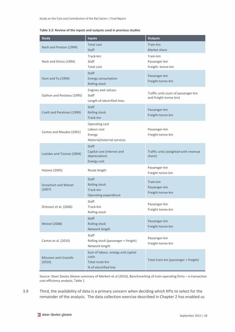
3.8 A recent study by Merkert et al (2010) presents a list of the main inputs and outputs (which
form the basis of any KPI) used in previous studies assessing the efficiency of national railway
systems. These are reported in Table 3.2 below. We have added the work carried out by
Mizutani and Uranishi (2010) to the list as this was not captured in the Merkert et al study,
and it provides some interesting indicators of total input costs and outputs.
10 Traffic units are calculated as a weighted average of passenger kilometres and freight tonne
kilometres. This relies on the assumption that average traffic unit costs are broadly constant. Otherwise, increasing productivity may simply mean that the railway is moving towards producing more freight traffic and less passenger traffic or vice versa. Hence, such a simple measure of output has significant shortcomings.
Study on the Cost and Contribution of the Rail Sector | Final Report
September 2015 | 28
Table 3.2: Review of the inputs and outputs used in previous studies
Study Inputs Outputs
Nash and Preston (1994) Total cost
Staff
Train-km
Market share
Nash and Shires (1994)
Track-km
Staff
Total cost
Train-km
Passenger-km
Freight -tonne-km
Oum and Yu (1994)
Staff
Energy consumption
Rolling stock
Passenger-km
Freight-tonne-km
Gathon and Pestieau (1995)
Engines and railcars
Staff
Length of electrified lines
Traffic units (sum of passenger-km and freight-tonne-km)
Coelli and Perelman (1999)
Staff
Rolling stock
Track-km
Passenger-km
Freight-tonne-km
Cantos and Maudos (2001)
Operating cost
Labour cost
Energy
Material/external services
Passenger-km
Freight-tonne-km
Loizides and Tsionas (2004)
Staff
Capital cost (interest and depreciation)
Energy cost
Traffic units (weighted with revenue share)
Hatano (2005) Route length Passenger-km
Freight tonne-km
Growitsch and Wetzel (2007)
Staff
Rolling stock
Track-km
Operating expenditure
Train-km
Passenger-km
Freight-tonne-km
Driessen et al. (2006)
Staff
Track-km
Rolling stock
Passenger-km
Freight-tonne-km
Wetzel (2008)
Staff
Rolling stock
Network length
Passenger-km
Freight-tonne-km
Cantos et al. (2010)
Staff
Rolling stock (passenger + freight)
Network length
Passenger-km
Freight-tonne-km
Mizutani and Uranishi (2010)
Sum of labour, energy and capital costs
Total route km
% of electrified line
Total train-km (passenger + freight)
Source: Steer Davies Gleave summary of Merkert et al (2010), Benchmarking of train operating firms – a transaction cost efficiency analysis, Table 1
3.9 Third, the availability of data is a primary concern when deciding which KPIs to select for the
remainder of the analysis. The data collection exercise described in Chapter 2 has enabled us

Study on the Cost and Contribution of the Rail Sector | Final Report
September 2015 | 29
to compile a large dataset. However, as noted in paragraph 2.11 there are gaps and
limitations. Gaps arise mainly in time-series data, with the result that it is not possible to
observe a specific KPI for every Member State for each year over the period 2003-2012.
3.10 There are also limitations relating to both the quality of data and the impact of external
influences. For instance, total track length may be an imprecise measure of productive capital
stock in Member States with a network comprised largely of assets nearing the end of their
economic life. A potential alternative would be to use the length of electrified lines, but this
measure is heavily influenced by the legacy of previous policy decisions and the availability of
investment funds.
3.11 Another measure subject to limitations is the value of subsidy. For example, a network that
benefits from substantial capital investment may require less maintenance expenditure and,
as a result, attract a lower level of operating subsidy. However, this apparently low level of
public resources used to support operations may be more than offset by public funding of
capital investment.
3.12 The primary and secondary KPIs considered in subsequent phases of the study have been
developed in the light of the three criteria described above (adherence to policy goals,
literature review and data availability). They are:
Primary KPIs
Track utilisation (train kilometres/track kilometres)
Passenger train utilisation (passenger kilometres/passenger rolling stock)
Freight train utilisation (freight tonne kilometres/freight rolling stock)
Secondary KPIs
Cost efficiency 1 (train kilometres/total operating costs)
Cost efficiency 2 (passenger kilometres/passenger operating costs)
Cost efficiency 3 (freight tonne kilometres/freight operating costs)
Staff efficiency (train kilometres/employees).
KPI analysis
3.13 As with all benchmarking activities, comparing the performance of rail systems across Member
States is not straightforward and any results should be interpreted with care. Benchmarking
simply compares outturn figures between observations and does not take into account the
broad range of micro and macro factors that may have contributed to a given level of
performance, and whether these are one-off or ongoing factors (e.g. outsourcing of labour).
Nor does benchmarking contribute to resolving any of the potential issues identified.
Notwithstanding these qualifications, by considering a broad range of performance measures
for each Member State it is possible to identify insights into the operating practices and
relative strengths and weaknesses of each railway system under consideration.
3.14 In order to develop hypotheses about the relative performance of rail systems across Member
States, we calculated and analysed relationships between combinations of primary and
secondary KPIs, together with a range of other explanatory variables. Bivariate analysis of this
nature allows investigation of how efficiency (as measured by primary KPIs) for a particular
Member State may be correlated with changes in secondary KPIs and/or exogenous factors.
The observed correlation between indicators does not imply causality, but indicates
relationships to be explored further in the subsequent clustering and data envelopment
analysis exercises. This section begins with a brief commentary on recent trends in KPIs and
then summarises the most useful evidence identified through correlation analysis. Detailed
outputs by Member State are provided in Appendix B.

Study on the Cost and Contribution of the Rail Sector | Final Report
September 2015 | 30
Trends in Key Performance Indicators
Track utilisation
3.15 As shown in Figure 3.1 there was a noticeable difference between Western and Eastern
Europe in track utilisation growth over the period 2007-2012. Although it fell in some Member
States, track utilisation in Western Europe grew by an average 8%, with the Netherlands (30%)
experiencing the largest increase. Track utilisation in Eastern Europe fell by an average of
10%, with the largest decreases in Greece and Estonia, where track utilisation fell by more
than 30% and 60% respectively.
Figure 3.1: Change in Track Utilisation (2007 to 2012) – train kilometres per track kilometre
Source: SDG analysis
Passenger train utilisation
3.16 As with track train utilisation, there was a contrast between Western and Eastern Europe in
passenger train utilisation growth over the period 2007-2012. Figure 3.2 indicates that
passenger train utilisation increased by an average of 8% in Western Europe over the period
2007-2012, with only Italy and Ireland experiencing a reduction. In Eastern Europe growth
was more varied, with Slovakia and Lithuania experiencing increases of more than 30% and
-3%
-23%
6%
17%
17%
-64%
-6%
-38%
-11%
2%
-18%
-10%
27%
20%
-15%
30%
18%
5%
0%
4%
17%
17%
-80% -60% -40% -20% 0% 20% 40%
BE
BG
CZ
DK
DE
EE
IE
EL
ES
FR
HR
IT
LV
LT
LU
HU
NL
AT
PL
PT
RO
SI
SK
FI
SE
UK
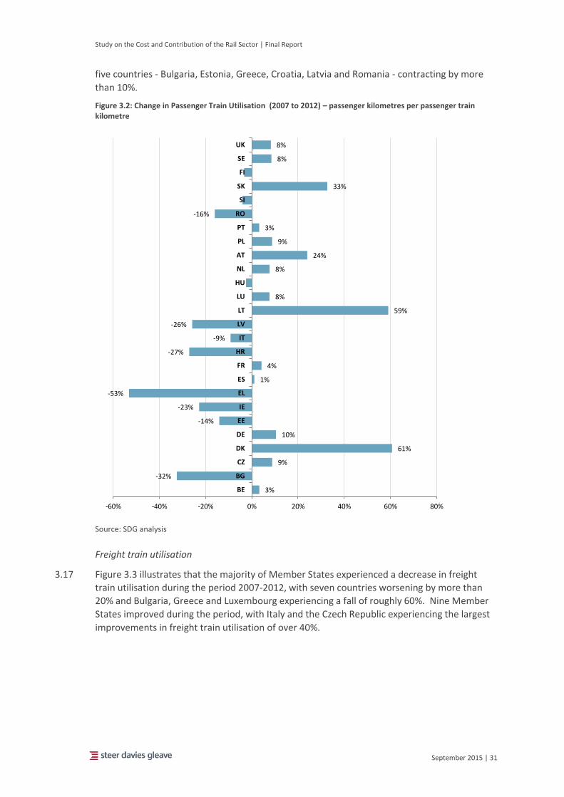
Study on the Cost and Contribution of the Rail Sector | Final Report
September 2015 | 31
five countries - Bulgaria, Estonia, Greece, Croatia, Latvia and Romania - contracting by more
than 10%.
Figure 3.2: Change in Passenger Train Utilisation (2007 to 2012) – passenger kilometres per passenger train kilometre
Source: SDG analysis
Freight train utilisation
3.17 Figure 3.3 illustrates that the majority of Member States experienced a decrease in freight
train utilisation during the period 2007-2012, with seven countries worsening by more than
20% and Bulgaria, Greece and Luxembourg experiencing a fall of roughly 60%. Nine Member
States improved during the period, with Italy and the Czech Republic experiencing the largest
improvements in freight train utilisation of over 40%.
3%
-32%
9%
61%
10%
-14%
-23%
-53%
1%
4%
-27%
-9%
-26%
59%
8%
8%
24%
9%
3%
-16%
33%
8%
8%
-60% -40% -20% 0% 20% 40% 60% 80%
BE
BG
CZ
DK
DE
EE
IE
EL
ES
FR
HR
IT
LV
LT
LU
HU
NL
AT
PL
PT
RO
SI
SK
FI
SE
UK

Study on the Cost and Contribution of the Rail Sector | Final Report
September 2015 | 32
Figure 3.3: Change in Freight Train Utilisation (2007 to 2012) – freight tonne kilometres per freight train kilometre
Source: SDG analysis
Secondary KPIs
3.18 As shown in Table 3.3 there has been considerable variation in the performance of Member
States against a range of secondary KPIs. At a system-wide level, there has been a significant
reduction in the number of train kilometres (freight and passenger combined) per unit of
operating cost expenditure, with only six Member States demonstrating any improvement.
Similar trends are observed when we compare passenger and freight tonne kilometres to
passenger and freight operating costs respectively, with the deterioration in freight cost
efficiency on average greater than that for passenger rail. This is unsurprising since in each
case the denominator of the KPI is a cost measure that is derived from the same source.
3.19 In contrast, when comparing outputs to the number of employees we observe improvements
in staff efficiency across 18 Member States. While there has been a modest reduction of
44,000 (or 4%) employees in the EU rail sector between 2007 and 2012, this is insufficient to
explain the discrepancy between physical and financial measures of efficiency. Changes to
wage rates may explain some of the discrepancy, but over the period in question wage growth
was subdued due to the ongoing impact of the financial crisis. Alternatively, deterioration in
7%
-58%
54%
28%
-17%
-33%
25%
-62%
-17%
-27%
50%
3%
-62%
-8%
-37%
-7%
5%
-13%
-37%
23%
-17%
2%
21%
-80% -60% -40% -20% 0% 20% 40% 60%
BE
BG
CZ
DK
DE
EE
IE
EL
ES
FR
HR
IT
LV
LT
LU
HU
NL
AT
PL
PT
RO
SI
SK
FI
SE
UK
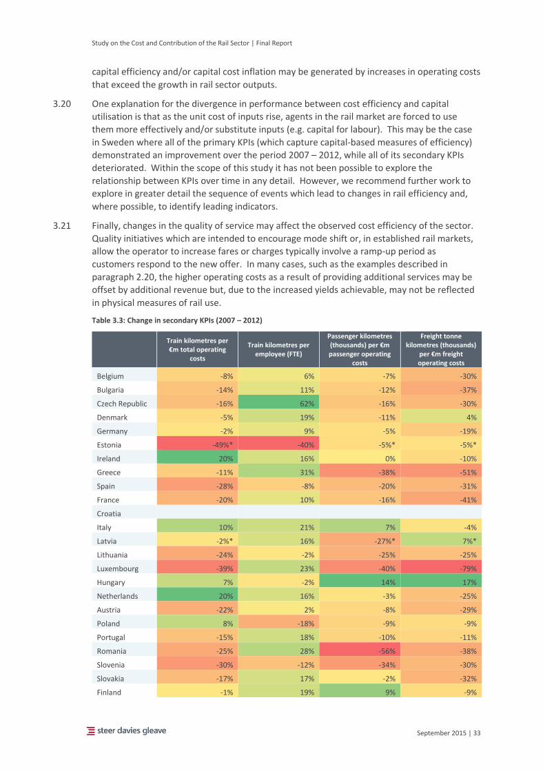
Study on the Cost and Contribution of the Rail Sector | Final Report
September 2015 | 33
capital efficiency and/or capital cost inflation may be generated by increases in operating costs
that exceed the growth in rail sector outputs.
3.20 One explanation for the divergence in performance between cost efficiency and capital
utilisation is that as the unit cost of inputs rise, agents in the rail market are forced to use
them more effectively and/or substitute inputs (e.g. capital for labour). This may be the case
in Sweden where all of the primary KPIs (which capture capital-based measures of efficiency)
demonstrated an improvement over the period 2007 – 2012, while all of its secondary KPIs
deteriorated. Within the scope of this study it has not been possible to explore the
relationship between KPIs over time in any detail. However, we recommend further work to
explore in greater detail the sequence of events which lead to changes in rail efficiency and,
where possible, to identify leading indicators.
3.21 Finally, changes in the quality of service may affect the observed cost efficiency of the sector.
Quality initiatives which are intended to encourage mode shift or, in established rail markets,
allow the operator to increase fares or charges typically involve a ramp-up period as
customers respond to the new offer. In many cases, such as the examples described in
paragraph 2.20, the higher operating costs as a result of providing additional services may be
offset by additional revenue but, due to the increased yields achievable, may not be reflected
in physical measures of rail use.
Table 3.3: Change in secondary KPIs (2007 – 2012)
Train kilometres per €m total operating
costs
Train kilometres per employee (FTE)
Passenger kilometres (thousands) per €m passenger operating
costs
Freight tonne kilometres (thousands)
per €m freight operating costs
Belgium -8% 6% -7% -30%
Bulgaria -14% 11% -12% -37%
Czech Republic -16% 62% -16% -30%
Denmark -5% 19% -11% 4%
Germany -2% 9% -5% -19%
Estonia -49%* -40% -5%* -5%*
Ireland 20% 16% 0% -10%
Greece -11% 31% -38% -51%
Spain -28% -8% -20% -31%
France -20% 10% -16% -41%
Croatia
Italy 10% 21% 7% -4%
Latvia -2%* 16% -27%* 7%*
Lithuania -24% -2% -25% -25%
Luxembourg -39% 23% -40% -79%
Hungary 7% -2% 14% 17%
Netherlands 20% 16% -3% -25%
Austria -22% 2% -8% -29%
Poland 8% -18% -9% -9%
Portugal -15% 18% -10% -11%
Romania -25% 28% -56% -38%
Slovenia -30% -12% -34% -30%
Slovakia -17% 17% -2% -32%
Finland -1% 19% 9% -9%
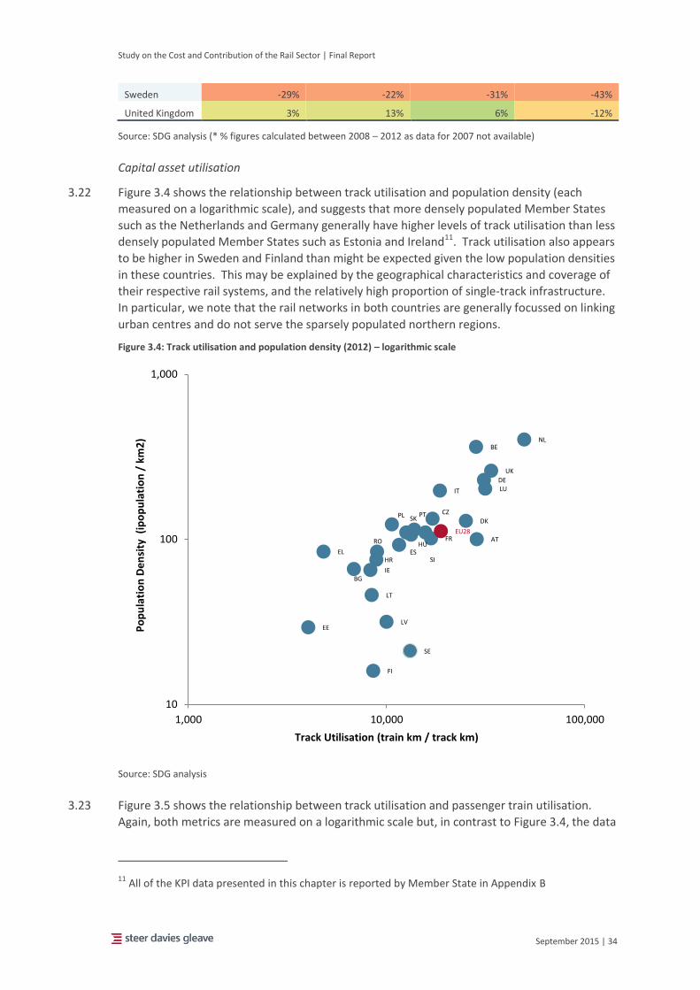
Study on the Cost and Contribution of the Rail Sector | Final Report
September 2015 | 34
Sweden -29% -22% -31% -43%
United Kingdom 3% 13% 6% -12%
Source: SDG analysis (* % figures calculated between 2008 – 2012 as data for 2007 not available)
Capital asset utilisation
3.22 Figure 3.4 shows the relationship between track utilisation and population density (each
measured on a logarithmic scale), and suggests that more densely populated Member States
such as the Netherlands and Germany generally have higher levels of track utilisation than less
densely populated Member States such as Estonia and Ireland11. Track utilisation also appears
to be higher in Sweden and Finland than might be expected given the low population densities
in these countries. This may be explained by the geographical characteristics and coverage of
their respective rail systems, and the relatively high proportion of single-track infrastructure.
In particular, we note that the rail networks in both countries are generally focussed on linking
urban centres and do not serve the sparsely populated northern regions.
Figure 3.4: Track utilisation and population density (2012) – logarithmic scale
Source: SDG analysis
3.23 Figure 3.5 shows the relationship between track utilisation and passenger train utilisation.
Again, both metrics are measured on a logarithmic scale but, in contrast to Figure 3.4, the data
11 All of the KPI data presented in this chapter is reported by Member State in Appendix B
BE
BG
CZ
DK
DE
EE
IE
EL ES
FR
HR
IT
LV
LT
LU
HU
NL
AT
PL PT
RO
SI
SK
FI
SE
UK
EU28
10
100
1,000
1,000 10,000 100,000
Po
pu
lati
on
De
nsi
ty (
ipo
pu
lati
on
/ k
m2
)
Track Utilisation (train km / track km)
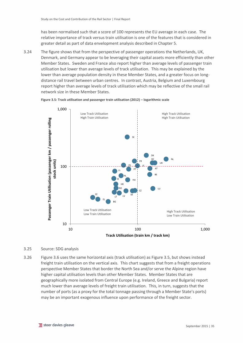
Study on the Cost and Contribution of the Rail Sector | Final Report
September 2015 | 35
has been normalised such that a score of 100 represents the EU average in each case. The
relative importance of track versus train utilisation is one of the features that is considered in
greater detail as part of data envelopment analysis described in Chapter 5.
3.24 The figure shows that from the perspective of passenger operations the Netherlands, UK,
Denmark, and Germany appear to be leveraging their capital assets more efficiently than other
Member States. Sweden and France also report higher than average levels of passenger train
utilisation but lower than average levels of track utilisation. This may be explained by the
lower than average population density in these Member States, and a greater focus on long-
distance rail travel between urban centres. In contrast, Austria, Belgium and Luxembourg
report higher than average levels of track utilisation which may be reflective of the small rail
network size in these Member States.
Figure 3.5: Track utilisation and passenger train utilisation (2012) – logarithmic scale
3.25 Source: SDG analysis
3.26 Figure 3.6 uses the same horizontal axis (track utilisation) as Figure 3.5, but shows instead
freight train utilisation on the vertical axis. This chart suggests that from a freight operations
perspective Member States that border the North Sea and/or serve the Alpine region have
higher capital utilisation levels than other Member States. Member States that are
geographically more isolated from Central Europe (e.g. Ireland, Greece and Bulgaria) report
much lower than average levels of freight train utilisation. This, in turn, suggests that the
number of ports (as a proxy for the total tonnage passing through a Member State’s ports)
may be an important exogenous influence upon performance of the freight sector.
BE
BG
CZ
DK
DE
EE
IE
EL
ES
FR
HR
IT
LV LT
LU
HU
NL
AT
PL
PT
RO
SK
FI
UK
SE
10
100
1,000
10 100 1,000
Pas
sen
ger
Trai
n U
tilis
atio
n (
pas
sen
ger
km /
pas
sen
ger
rolli
ng
sto
ck u
nit
s)
Track Utilisation (train km / track km)
Low Track Utilisation High Train Utilisation
High Track Utilisation High Train Utilisation
High Track Utilisation Low Train Utilisation
Low Track Utilisation Low Train Utilisation

Study on the Cost and Contribution of the Rail Sector | Final Report
September 2015 | 36
Figure 3.6: Track utilisation and freight train utilisation (2012) – logarithmic scale
Source: SDG analysis (note that Luxembourg is not shown in the chart as it lies outside the area illustrated)
Figure 3.7 shows the relationship between passenger track utilisation and freight track
utilisation using a logarithmic scale where a score of 100 represents the EU average for that
indicator12. This helps us to categorise Member States according to the main market served by
their railway network (passenger-centric, freight-centric or both). It is notable that most
Member States with higher than average passenger track utilisation are relatively high income,
Western European countries. However, those Member States with the very highest freight
track utilisation are the three Baltic States. The high utilisation rates are as a result of large
freight transit traffic volumes to Russia and other countries in the Commonwealth of
Independent States (CIS).
3.27 Figure 3.8 shows the same relationship on an absolute scale and suggests there may be a
trade-off between freight track utilisation and passenger track utilisation, as indicated by the
12 Care should be taken when comparing Figures 3.5 and 3.6 with Figures 3.7 and 3.8. The ‘track
utilisation’ metric is formulated differently whereby in the former figures it measures train kilometres per track kilometre while in the latter figures it measures passenger kilometres or freight kilometres per track kilometre.
BE
BG
CZ
DK
DE
EE
IE
EL
ES
FR
HR
IT
LV
LT
HU
NL
AT
PL PT
RO
SI
SK
FI
UK
SE
10
100
1,000
10 100 1,000
Fre
igh
t Tr
ain
Uti
lisat
ion
(to
nn
e k
m /
fre
igh
t ro
llin
g st
ock
un
its)
Track Utilisation (train km / track km)
Low Track Utilisation
Low Train Utilisation
High Track Utilisation
Low Train Utilisation
Low Track Utilisation
High Train Utilisation High Train Utilisation High Track Utilisation

Study on the Cost and Contribution of the Rail Sector | Final Report
September 2015 | 37
illustrative efficiency frontier13. This is unsurprising given that both types of operations often
use the same network and compete for scarce paths.
Figure 3.7: Passenger track utilisation and freight track utilisation (2012) – logarithmic scale
13 Note that the efficiency frontier has been shown for illustrative purposes only. No statistical tests
were carried out to determine the significance, nor test the functional form of this relationship.
BE
BG
CZ
DK
DE
EE
ES
FR
HR
IT
LV
LT
LU
HU
NL
AT
PL
PT
RO
SI
SK
FI UK
SE
10
100
1,000
10 100 1,000
Fre
igh
t Tr
ack
Uti
lisat
ion
(to
nn
e k
m /
tra
ck k
m)
Passenger Track Utilisation (passenger km / track km)
High Passenger Utilisation
High Freight Utilisation
High Passenger Utilisation
Low Freight Utilisation
Low Passenger Utilisation
Low Freight Utilisation
Low Passenger Utilisation
High Freight Utilisation
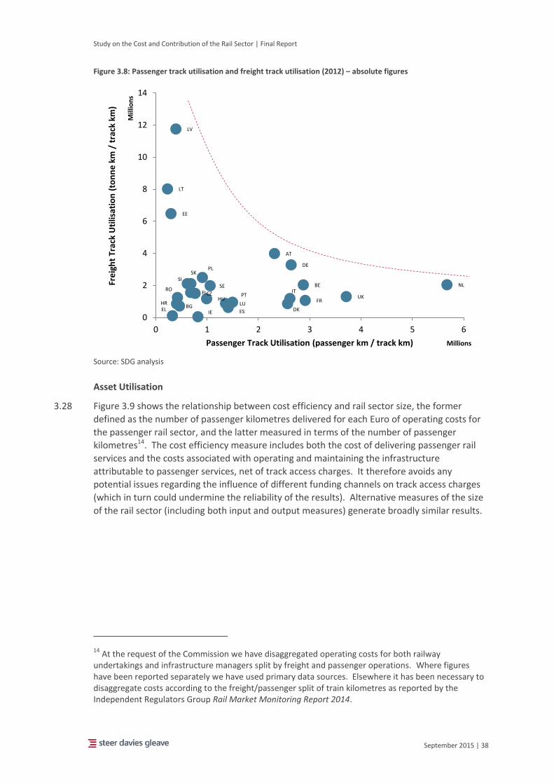
Study on the Cost and Contribution of the Rail Sector | Final Report
September 2015 | 38
Figure 3.8: Passenger track utilisation and freight track utilisation (2012) – absolute figures
Source: SDG analysis
Asset Utilisation
3.28 Figure 3.9 shows the relationship between cost efficiency and rail sector size, the former
defined as the number of passenger kilometres delivered for each Euro of operating costs for
the passenger rail sector, and the latter measured in terms of the number of passenger
kilometres14. The cost efficiency measure includes both the cost of delivering passenger rail
services and the costs associated with operating and maintaining the infrastructure
attributable to passenger services, net of track access charges. It therefore avoids any
potential issues regarding the influence of different funding channels on track access charges
(which in turn could undermine the reliability of the results). Alternative measures of the size
of the rail sector (including both input and output measures) generate broadly similar results.
14 At the request of the Commission we have disaggregated operating costs for both railway
undertakings and infrastructure managers split by freight and passenger operations. Where figures have been reported separately we have used primary data sources. Elsewhere it has been necessary to disaggregate costs according to the freight/passenger split of train kilometres as reported by the Independent Regulators Group Rail Market Monitoring Report 2014.
BE
BG
CZ
DK
DE
EE
IE EL ES
FR HR
IT
LV
LT
LU HU
NL
AT
PL
PT RO
SI SK
FI UK
SE
0
2
4
6
8
10
12
14
0 1 2 3 4 5 6
Fre
igh
t Tr
ack
Uti
lisat
ion
(to
nn
e k
m /
tra
ck k
m)
Mill
ion
s
Passenger Track Utilisation (passenger km / track km) Millions

Study on the Cost and Contribution of the Rail Sector | Final Report
September 2015 | 39
Figure 3.9: Cost efficiency and passenger km (2012) – logarithmic scale
Source: SDG analysis
3.29 The chart indicates a weak relationship between rail system size and efficiency, with larger
railway systems marginally more cost efficient than smaller ones. This, in turn, suggests that
economies of scale (and potentially network benefits) may play a relatively limited role in
delivering high levels of efficiency, and that relative efficiency is likely to be affected by a range
of factors other than scale.
3.30 The rail network in Germany delivered 88.4 billion passenger kilometres in 2012, 6.9
passenger kilometres for every Euro of operating costs spent. By contrast, France delivered
marginally higher passenger outputs of 89.1 billion passenger kilometres but at more than
twice the cost (3.3 passenger kilometres per € operating cost). In practice this is due, in part,
to the considerably larger labour force employed by the French railways (158,000) compared
to German railways (100,000).
3.31 While a number of smaller, Eastern European rail systems appear to deliver higher than
average passenger kilometres per unit of operating costs this may, in part, be an artefact of
the methodology used to disaggregate total operating costs into freight and passenger costs15.
15 By disaggregating total operating costs (for both operators and infrastructure managers) according to
the proportion of passenger and freight train kilometres, in those Member States where freight delivers a large proportion of total train kilometres relative to passenger-focussed rail systems it may be the case that the operating costs for the passenger railway are under-estimated.
BE
BG
CZ
DK
DE
EE
IE
EL
ES
FR
IT
LV
LT
LU
HU
NL
AT
PL
PT
RO SI SK
FI
UK
SE
0
1
2
3
4
5
6
7
8
9
10
100 1,000 10,000 100,000
Co
st E
ffic
ien
cy (
pas
sen
ger
kilo
me
tre
s /
€ p
asse
nge
r o
pe
rati
ng
cost
)
Passenger km (millions)

Study on the Cost and Contribution of the Rail Sector | Final Report
September 2015 | 40
Ireland, on the other hand, which has relatively small freight sector, provides a more direct
comparison to the larger Member States and appears to deliver high levels of rail patronage
relative to its operating costs.
Subsidies
3.32 Figure 3.10 illustrates the relationship between passenger revenues and total subsidies16.
These have been normalised using track kilometres as a scaling measure. The strong positive
correlation suggests that subsidy and revenue increase is in-line with each other and we note
that, in absolute terms, subsidies tend to be greater in large, higher income Member States.
From a purely financial perspective, we might have expected to observe a negative
relationship. In practice, however, this suggests either that:
Member States which provide a high-quality, high-frequency railway generate higher
levels of patronage and fare revenue (e.g. Netherlands);
Member States which generate high levels of patronage and revenue are willing to
subsidise higher quality rail services (e.g. United Kingdom); or
Some combination of the two points above (e.g. Germany).
Figure 3.10: Subsidy and revenue (2012) – logarithmic scale
16 Freight operations should, in principle, not be subsidised. They may, however, benefit indirectly from
the subsidies provided to infrastructure managers - higher subsidies to infrastructure managers lead to lower track access charges.
BE
BG
CZ
DK
DE
IE
EL
ES
FR
IT
LT
LU
HU
NL
AT
PL
PT
RO
SI SK
FI
UK
SE
10,000
100,000
1,000,000
1,000 10,000 100,000 1,000,000
Sub
sid
y p
er
trac
k ki
lom
etr
e (
€ /
km
)
Passenger revenue per track kilometre (€ / km)

Study on the Cost and Contribution of the Rail Sector | Final Report
September 2015 | 41
Source: SDG analysis (note that it has not been possible to obtain reliable revenue data for Estonia and Croatia. Latvia is not shown on the charts as it lies outside the area illustrated)
Conclusions
3.33 In carrying out this investigation it was notable how few relationships could be identified on a
bivariate basis, suggesting that the range of factors which affect the efficiency of rail networks
between Member States are many and/or the relationships are complex.
3.34 This chapter summarises the results of an extensive data mining exercise in which
relationships between primary KPIs and secondary KPIs/exogenous variables were explored in
depth. The purpose of this exercise was to develop hypotheses regarding the variables that
are likely to have greatest influence upon the efficiency of the rail sector, and to test these
hypotheses through the subsequent clustering (exogenous) and data envelopment analysis
(endogenous) exercises.

Study on the Cost and Contribution of the Rail Sector | Final Report
September 2015 | 42
4 Clustering analysis Overview
4.1 The primary goal of the clustering exercise is to control for the impact of exogenous factors
that are beyond the control of managers and policy-makers and can only be changed over the
long term, if at all. This allows us to focus on differences in industry performance that are
explained by endogenous factors, including investment and innovation. We therefore cluster
Member States into subsets consisting of countries for which the impact of exogenous factors
is expected to be broadly similar. In analytical terms, the aim is to minimise the similarity
between the subsets while maximising the similarity between countries within each subset.
This will:
Establish a basic categorisation of national rail systems for the purpose of the current
analysis and to inform future benchmarking exercises at the EU level; and
Increase the discriminatory power of the subsequent efficiency analysis by reducing the
heterogeneity of the sample.
4.2 Clustering analysis is intended to provide a bridge between the bivariate analysis of key
performance indicators described in Chapter 3 and the more formal measurement of
efficiency generated by the data envelopment analysis described in Chapter 5.
Clustering principles
4.3 The choice of exogenous variables to include within the clustering analysis was informed by:
Empirical evidence;
Economic theory; and
Investigation of KPIs discussed in the previous chapter.
4.4 In order to identify relevant exogenous factors we reviewed a selection of academic and
industry literature on the determinants of utilisation and efficiency of national rail services
(e.g. mode share, productivity) and isolated the exogenous factors that appear most
frequently. From our review of the literature (summarised in Table 4.1), we concluded that:
Measures of population density (inhabitants per km2) and wealth (GDP per capita) should
be included as explanatory variables within the clustering analysis;
Where available, specific measures closely related to rail (e.g. the number of major ports
linked by rail) are preferred to broader definitions such as the length of the coastline and
should be included;
The external cost of car travel is highly correlated with GDP per capita and should not be
included in the analysis;
While the existing length/density of the rail network is arguably endogenous over the long
term, we consider that it should be treated as exogenous given the timeframe of our
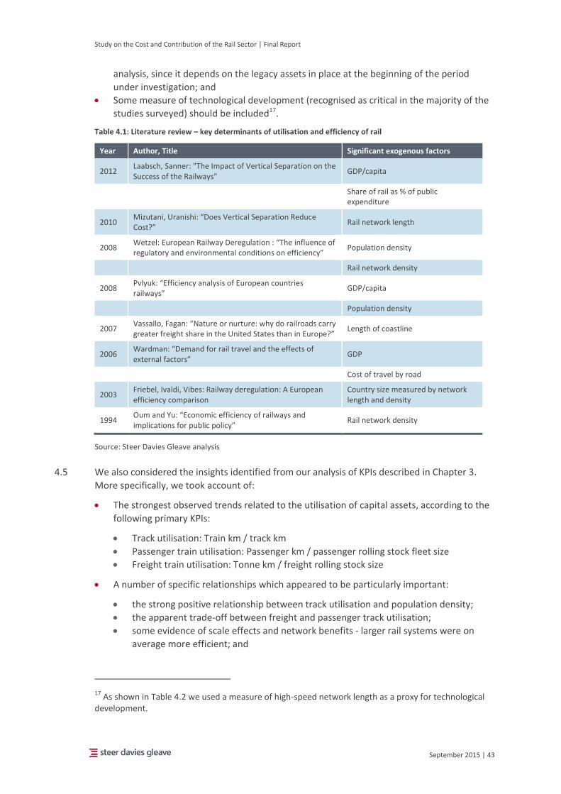
Study on the Cost and Contribution of the Rail Sector | Final Report
September 2015 | 43
analysis, since it depends on the legacy assets in place at the beginning of the period
under investigation; and
Some measure of technological development (recognised as critical in the majority of the
studies surveyed) should be included17.
Table 4.1: Literature review – key determinants of utilisation and efficiency of rail
Year Author, Title Significant exogenous factors
2012 Laabsch, Sanner: "The Impact of Vertical Separation on the Success of the Railways"
GDP/capita
Share of rail as % of public expenditure
2010 Mizutani, Uranishi: “Does Vertical Separation Reduce Cost?”
Rail network length
2008 Wetzel: European Railway Deregulation : “The influence of regulatory and environmental conditions on efficiency”
Population density
Rail network density
2008 Pvlyuk: “Efficiency analysis of European countries railways”
GDP/capita
Population density
2007 Vassallo, Fagan: “Nature or nurture: why do railroads carry greater freight share in the United States than in Europe?”
Length of coastline
2006 Wardman: “Demand for rail travel and the effects of external factors”
GDP
Cost of travel by road
2003 Friebel, Ivaldi, Vibes: Railway deregulation: A European efficiency comparison
Country size measured by network length and density
1994 Oum and Yu: “Economic efficiency of railways and implications for public policy”
Rail network density
Source: Steer Davies Gleave analysis
4.5 We also considered the insights identified from our analysis of KPIs described in Chapter 3.
More specifically, we took account of:
The strongest observed trends related to the utilisation of capital assets, according to the
following primary KPIs:
Track utilisation: Train km / track km
Passenger train utilisation: Passenger km / passenger rolling stock fleet size
Freight train utilisation: Tonne km / freight rolling stock size
A number of specific relationships which appeared to be particularly important:
the strong positive relationship between track utilisation and population density;
the apparent trade-off between freight and passenger track utilisation;
some evidence of scale effects and network benefits - larger rail systems were on
average more efficient; and
17 As shown in Table 4.2 we used a measure of high-speed network length as a proxy for technological
development.

Study on the Cost and Contribution of the Rail Sector | Final Report
September 2015 | 44
The limited evidence relating to the utilisation of non-capital assets generated through
our examination of KPIs.
4.6 On the basis of these exercises, the exogenous variables described Table 4.2 were used in the
clustering exercise as the measures against which the similarity between Member States
would be estimated.
Table 4.2: Clustering variables
Passenger Freight Comments
Population Affects the overall level of activity in the economy
Area Rail has a particular advantage over medium distances
Population density Goods carried by freight not typically affected by settlement patterns
Urban population (%) As above
GDP per capita Direct measure of economic activity
Border countries (#) Long-distance transit freight supports international trade
Ports connected by rail Majority of goods conveyed by freight travel to/from sea ports
Network length Direct measure of network size
High speed network length Indirect measure of innovation
4.7 The number of clusters needs to be large enough to ensure that it is possible to differentiate
between them, while at the same time the number of observations within each cluster needs
to be large enough to ensure the data envelopment analysis generates meaningful estimates
of relative efficiency between Member States. In addition, while clustering should be based
on the most recent data available, it is important to avoid allocating Member States to clusters
based on what might be one-off events in a given year. We have reviewed historical series
and, where outliers were found, taken an average across a three year time period.
Clustering methodology
Trial methodologies
4.8 While it is necessary to use an approach that is rooted in evidence, the methodology
underpinning the definition of clusters should also be transparent and robust. Using the
principles described above as a guide, we considered and applied a number of alternative
clustering techniques before identifying a preferred approach. More specifically, we
considered three distinct yet complementary methodologies that appeared promising but
which were ultimately discarded. These were:
Regression modelling;
Hierarchical partitioning; and
Expert review.
4.9 Given the limitations of these approaches, as reported in Appendix B, we concluded that there
would be a significant risk of misallocation of a Member State to a cluster if any one of them
were applied in isolation. This, in turn, could have significant implications for the results of the
scenario assessment exercise (for example, if the best performing observation in a given
cluster were misallocated and became the worst performing Member State in another). We
therefore identified an alternative approach, using non-parametric analysis, which places
greater weight on the use of data to determine cluster boundaries.
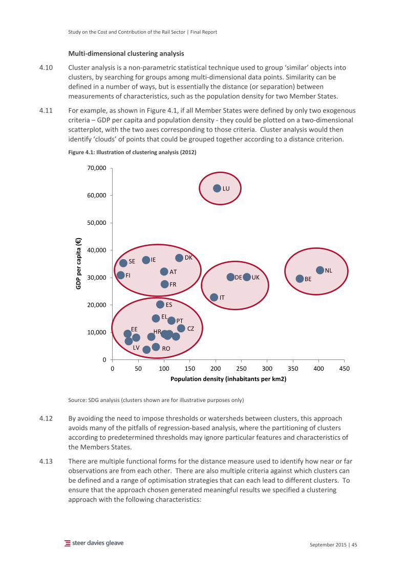
Study on the Cost and Contribution of the Rail Sector | Final Report
September 2015 | 45
Multi-dimensional clustering analysis
4.10 Cluster analysis is a non-parametric statistical technique used to group ‘similar’ objects into
clusters, by searching for groups among multi-dimensional data points. Similarity can be
defined in a number of ways, but is essentially the distance (or separation) between
measurements of characteristics, such as the population density for two Member States.
4.11 For example, as shown in Figure 4.1, if all Member States were defined by only two exogenous
criteria – GDP per capita and population density - they could be plotted on a two-dimensional
scatterplot, with the two axes corresponding to those criteria. Cluster analysis would then
identify ‘clouds’ of points that could be grouped together according to a distance criterion.
Figure 4.1: Illustration of clustering analysis (2012)
Source: SDG analysis (clusters shown are for illustrative purposes only)
4.12 By avoiding the need to impose thresholds or watersheds between clusters, this approach
avoids many of the pitfalls of regression-based analysis, where the partitioning of clusters
according to predetermined thresholds may ignore particular features and characteristics of
the Members States.
4.13 There are multiple functional forms for the distance measure used to identify how near or far
observations are from each other. There are also multiple criteria against which clusters can
be defined and a range of optimisation strategies that can each lead to different clusters. To
ensure that the approach chosen generated meaningful results we specified a clustering
approach with the following characteristics:
BE
CZ
DK
DE
EE
IE
EL
ES
FR
HR
IT
LV
LU
NL AT
PT
RO
FI UK
SE
0
10,000
20,000
30,000
40,000
50,000
60,000
70,000
0 50 100 150 200 250 300 350 400 450
GD
P p
er
cap
ita
(€)
Population density (inhabitants per km2)

Study on the Cost and Contribution of the Rail Sector | Final Report
September 2015 | 46
Hierarchical: the set of clusters generated is nested and organised as a tree. Each node
(cluster) in the tree is the union of its branches (sub-clusters) and the root of the tree is
the cluster containing all the objects (in this case Member States).
Exclusive: Member States cannot belong to more than one cluster. Each object is
assigned to a single cluster only.
Complete: Every Member State is assigned to a cluster.
4.14 Given the requirements described above, and to avoid predetermining the number of clusters,
we used agglomerative hierarchical clustering techniques, which tend to be the most common
methods used in practice18. Agglomerative clustering methods begin with every object
(Member State) defined as an individual cluster, following which, at each iterative step, the
closest pairs of clusters are merged.
4.15 More specifically, for this study we have used an agglomerative technique known as Ward’s
minimum variance method19. This aims to minimise the total ‘within cluster’ variance across
all the clusters and ensures the clusters are compact with a good level of similarity between
observations in the same cluster. The distance measure used to calculate the distance
between clusters is given by the following formula20:
[∑(𝑥𝑖,𝑝−𝑥𝑗,𝑝)2
𝑃
𝑝=1
]
12⁄
4.16 A hierarchical clustering can be displayed graphically using a tree-like diagram called a
dendrogram, which shows both the cluster/sub-cluster relationship and the order in which the
clusters were merged. Figure 4.2 shows an example dendrogram (and its associated nested
cluster diagram) for a set of four two-dimensional points. Dendrograms showing the results of
the clustering analysis carried out for this study are provided in Appendix D.
18 See Introduction to Data Mining (Tan, Steinbach and Kumar, 2006)
19 See Ward, J.H. (1963) Hierarchical Grouping to Optimize and Objective Function, Journal of the
American Statistical Association
20 We also considered an alternative distance measure (the squared Euclidean) but this had no impact
upon the results of the clustering analysis.

Study on the Cost and Contribution of the Rail Sector | Final Report
September 2015 | 47
Figure 4.2: Dendrogram and nested cluster examples
Application and results
4.17 Based on the measures reported in Table 4.2, we identified combinations of variables to be
used in the clustering exercise. In doing so we carried out both freight and passenger-oriented
clustering exercises using variables that are expected to affect the efficiency of that sector (for
example, we would not expect the number of ports linked by rail to have a material influence
on the efficiency of the passenger railway).
Table 4.3: Summary of clustering analysis
Passenger Freight
Clustering model 1 2 3 4 5 6 7 8 9
Population
Area
Population density
Urban population (%)
GDP per capita
Border countries (#)
Ports connected by rail
Network length
High speed network length
4.18 In carrying out the clustering analysis, we identified the following features and trends. For the
passenger-based clustering exercises (1 to 5):
Separate measures of population and land mass strongly dominate all other variables.
This leads to very stable (but counterintuitive) clusters.
Using a measure of population density is preferable to using separate measures of
population and land mass (area) and fits with insights drawn from the KPI analysis
exercise reported in Chapter 3.
Clustering based on population density (among other measures) consistently identified
Luxembourg as an outlier – this may be a result of both Luxembourg’s size and the
divergence between resident population and employment.
Including measures of network length led to an allocation of Member States to clusters
according to their size. These results were considered preferable to those derived using
an approach that ignored network size, as network length can be regarded as a proxy for
scale effects.
MS1 MS
2 MS
3 MS
4
MS1
MS2
MS3
MS4
Dendrogram Nested cluster diagram

Study on the Cost and Contribution of the Rail Sector | Final Report
September 2015 | 48
The specification of the high-speed network length (in absolute or proportionate terms)
had no impact on the results of the clustering exercise.
4.19 For the freight-based clustering exercises (6 to 9):
As with the passenger-focussed clustering tests, the inclusion of land mass within the
analysis strongly dominates all other variables. In the presence of a land mass variable,
the inclusion of measures that describe the number of ports linked by rail or number of
border countries did not affect the specification of clusters.
Removing measures of land mass from the clustering analysis increases the influence of
those measures thought to be more closely linked to freight performance, such as the
number of ports and border countries.
Again, Luxembourg was consistently identified as an outlier.
4.20 For each of the clustering exercises, we sought to identify four to six clusters21. As labelled in
Figure 4.3, clustering exercises four (passenger-based) and eight (freight-based) generated the
most stable and intuitive results and are presented in Table 4.4 and Table 4.5 below. The
colour coding represents the allocation of Member States to clusters. A full set of clustering
outputs, including the associated dendrograms is provided in Appendix D.
Table 4.4: Clustering outputs (passenger) – test 4
6 clusters 5 clusters 4 clusters
Belgium
Denmark Ireland Netherlands Austria Finland Luxembourg Germany
France Spain
Italy Sweden UK Poland
Hungary Czech Republic Bulgaria Romania Estonia
Greece Croatia Latvia Lithuania Slovenia Slovakia Portugal
Source: SDG analysis
21 Note that, due to the hierarchical nature of the clustering methodology, in order to generate one of
the clusters identified in the ‘4-cluster’ specification, two cluster from ‘5-cluster’ specification must be
combined, and vice-versa.
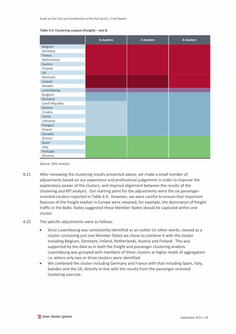
Study on the Cost and Contribution of the Rail Sector | Final Report
September 2015 | 49
Table 4.5: Clustering outputs (freight) – test 8
6 clusters 5 clusters 4 clusters
Belgium
Germany France Netherlands Austria Finland UK Denmark
Ireland Sweden Luxembourg Bulgaria
Romania Czech Republic
Estonia Croatia Latvia Lithuania Hungary Poland Slovakia Greece
Spain Italy Portugal Slovenia
Source: SDG analysis
4.21 After reviewing the clustering results presented above, we made a small number of
adjustments based on our experience and professional judgement in order to improve the
explanatory power of the clusters, and improve alignment between the results of the
clustering and KPI analysis. Our starting point for the adjustments were the six passenger-
oriented clusters reported in Table 4.4. However, we were careful to ensure that important
features of the freight market in Europe were retained, for example, the dominance of freight
traffic in the Baltic States suggested these Member States should be captured within one
cluster.
4.22 The specific adjustments were as follows:
Since Luxembourg was consistently identified as an outlier (in other words, classed as a
cluster containing just one Member State) we chose to combine it with the cluster
including Belgium, Denmark, Ireland, Netherlands, Austria and Finland. This was
supported by the data as in both the freight and passenger clustering analysis
Luxembourg was grouped with members of these clusters at higher levels of aggregation
i.e. where only two or three clusters were identified.
We combined the cluster including Germany and France with that including Spain, Italy,
Sweden and the UK, directly in-line with the results from the passenger-oriented
clustering exercise.

Study on the Cost and Contribution of the Rail Sector | Final Report
September 2015 | 50
We split the large residual cluster according to the 6-cluster results from the passenger-
oriented clustering exercise22.
4.23 The final set of clusters are presented in Table 4.6.
Table 4.6: Final clusters
Cluster A Cluster B Cluster C Cluster D
Belgium Germany Poland Estonia
Denmark France Hungary Greece
Ireland Spain Czech Republic Croatia
Netherlands Italy Bulgaria Latvia
Austria Sweden Romania Lithuania
Finland UK Slovenia
Luxembourg Slovakia
Portugal
4.24 Upon initial inspection, the clusters may be broadly categorised as follows:
Cluster A: Relatively small, high income western European countries;
Cluster B: Large, populous western European countries;
Cluster C: Medium-sized, lower income central and eastern European countries; and
Cluster D: Baltic states and Mediterranean fringe countries with lower incomes.
4.25 Figure 4.3 summarises the size of the clusters obtained above with respect to population, GDP,
passenger-kilometres and freight tonne kilometres. While clusters A, C and D are broadly of
the same size, particularly with respect to population, cluster B is significantly larger. This is
unsurprising since cluster B includes Europe’s five largest economies. It is notable that the
variable with least variation between clusters is freight tonne kilometres, consistent with the
observation that the rail networks of the larger Member States captured within cluster B are
focused primarily on the provision of passenger rather than freight services.
22
Since 78% of the market for rail services in the European Union is passenger traffic, we have placed greater, but not exclusive, weight on the findings of the passenger-based clustering exercise

Study on the Cost and Contribution of the Rail Sector | Final Report
September 2015 | 51
Figure 4.3: Relative size of clusters by GDP, population, passenger km and freight tonne km (2012)
Source: SDG analysis
4.26 Figure 4.4 and Figure 4.5 examine a subset of the variables used to inform the clustering
exercise in more detail. It is clear from Figure 4.4 that the Member States that make up
clusters A and B have significantly higher income per capita than those Member States in
clusters C and D. However, as Figure 4.5 indicates, the countries in cluster A are significantly
smaller than those in cluster B and this is reflected in the size of their rail network. The rail
networks within cluster C are generally larger than those in cluster D, but there is considerable
variation between individual Member States.
0.0%
10.0%
20.0%
30.0%
40.0%
50.0%
60.0%
70.0%
80.0%
GDP Population Pax km Tonne km
Cluster A Cluster B Cluster C Cluster D

Study on the Cost and Contribution of the Rail Sector | Final Report
September 2015 | 52
Figure 4.4: GDP per capita by Member State and cluster (2012)
Figure 4.5: Rail network length by Member State and cluster (2012)
Source: SDG analysis
4.27 In order to understand the extent to which the clustering analysis has captured variations in
the relative performance of Member State rail systems (as measured by primary KPIs), Figure
4.6 and Figure 4.7 replicate Figure 3.5 and Figure 3.6 with the data points coloured according
to the cluster to which the Member State is assigned. If the data points for a given cluster are
located close to each other, we can infer that exogenous variables account for a large
proportion of the variation between Member States. Conversely, if the data points remain
-
10,000
20,000
30,000
40,000
50,000
60,000
70,000
BE DK IE LU NL AT FI DE ES FR IT SE UK BG CZ HU PL RO EE EL HR LV LT PT SI SK
Cluster A Cluster B Cluster C Cluster D
GD
P p
er
cap
ita
(€)
-
5,000
10,000
15,000
20,000
25,000
30,000
35,000
40,000
BE DK IE LU NL AT FI DE ES FR IT SE UK BG CZ HU PL RO EE EL HR LV LT PT SI SK
Cluster A Cluster B Cluster C Cluster D
Ne
two
rk le
ngt
h (
km)

Study on the Cost and Contribution of the Rail Sector | Final Report
September 2015 | 53
dispersed, this suggests that endogenous (and potentially unobserved) factors have a greater
role to play in explaining relative performance.
Figure 4.6: Passenger train utilisation versus total track utilisation by Member State and cluster (2012)
Source: SDG analysis
4.28 Typically, high levels of passenger track utilisation are often representative of extensive public
service obligations and, due to the requirement to deliver service level commitments, can
often lead to lower levels of train utilisation. Figure 4.6 suggests that the exogenous variables
used in the clustering exercise perform well in explaining variation in the performance of
Member States in clusters C and D against both passenger train utilisation and track utilisation.
4.29 In clusters A and B, however, the explanatory power of these variables is more mixed.
Observations for cluster B are relatively tightly grouped against the train utilisation metric, but
there is considerably greater variation against the track utilisation measure. The converse
appears to be true for cluster A, where performance against the track utilisation measure is
uniform (with Ireland and Finland obvious outliers) but there is greater variation in
performance against the train utilisation measure.
4.30 In contrast, Figure 4.7 suggests that the exogenous variables used to cluster Member States
are better for explaining variation in freight train utilisation for clusters A and B than for
clusters C and D. This is likely to be a consequence of the significant variation in the relative
importance of freight to the overall market in the Member States in clusters C and D, and the
greater weight placed upon the results of the passenger clustering exercise when determining
the final clusters.
BE
BG
CZ
DK
DE
EE
IE
EL
ES
FR
HR
IT
LV LT
LU
HU
NL
AT
PL
PT
RO SK
FI
UK
SE
10
100
1,000
10 100 1,000
Pas
sen
ger
Trai
n U
tilis
atio
n (
pas
sen
ger
km /
pas
sen
ger
rolli
ng
sto
ck u
nit
s)
Track Utilisation (train km / track km)
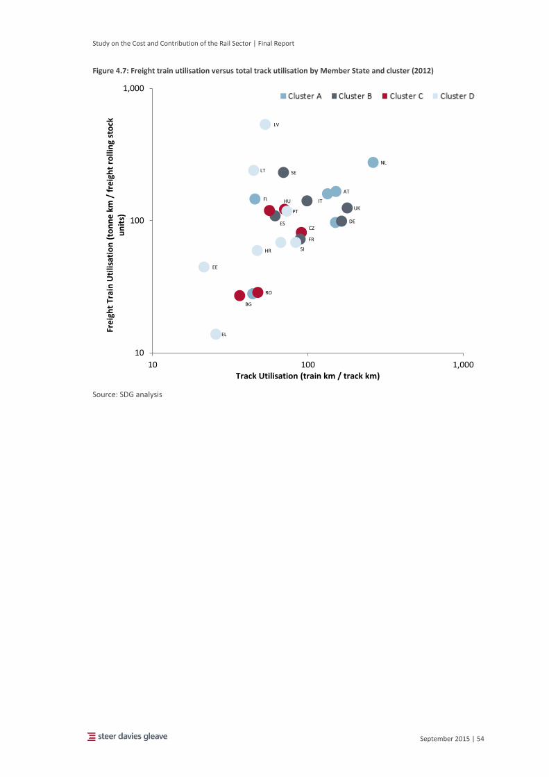
Study on the Cost and Contribution of the Rail Sector | Final Report
September 2015 | 54
Figure 4.7: Freight train utilisation versus total track utilisation by Member State and cluster (2012)
Source: SDG analysis
BG
CZ DE
EE
EL
ES
FR
HR
IT
LV
LT
HU
NL
AT
PT
RO
SI
FI
UK
SE
10
100
1,000
10 100 1,000
Fre
igh
t Tr
ain
Uti
lisat
ion
(to
nn
e k
m /
fre
igh
t ro
llin
g st
ock
u
nit
s)
Track Utilisation (train km / track km)
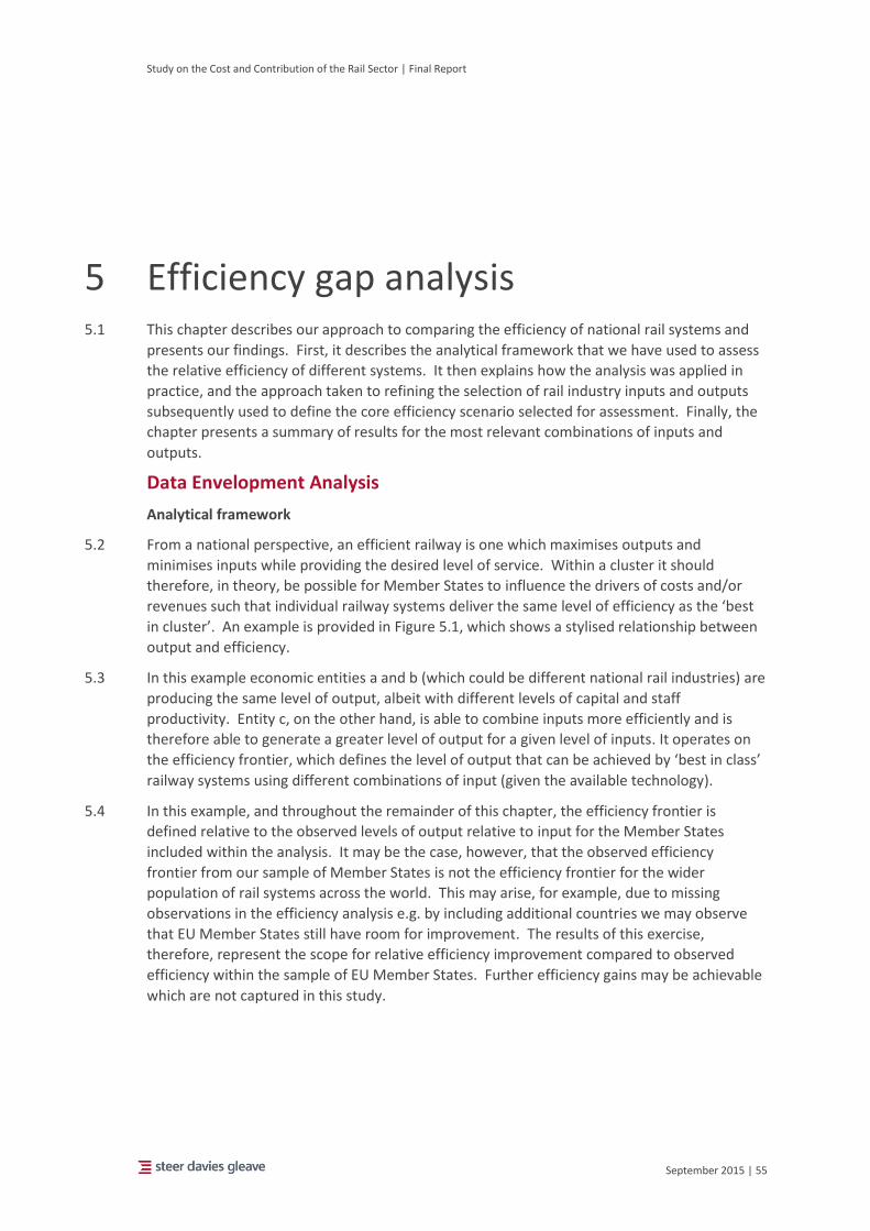
Study on the Cost and Contribution of the Rail Sector | Final Report
September 2015 | 55
5 Efficiency gap analysis 5.1 This chapter describes our approach to comparing the efficiency of national rail systems and
presents our findings. First, it describes the analytical framework that we have used to assess
the relative efficiency of different systems. It then explains how the analysis was applied in
practice, and the approach taken to refining the selection of rail industry inputs and outputs
subsequently used to define the core efficiency scenario selected for assessment. Finally, the
chapter presents a summary of results for the most relevant combinations of inputs and
outputs.
Data Envelopment Analysis
Analytical framework
5.2 From a national perspective, an efficient railway is one which maximises outputs and
minimises inputs while providing the desired level of service. Within a cluster it should
therefore, in theory, be possible for Member States to influence the drivers of costs and/or
revenues such that individual railway systems deliver the same level of efficiency as the ‘best
in cluster’. An example is provided in Figure 5.1, which shows a stylised relationship between
output and efficiency.
5.3 In this example economic entities a and b (which could be different national rail industries) are
producing the same level of output, albeit with different levels of capital and staff
productivity. Entity c, on the other hand, is able to combine inputs more efficiently and is
therefore able to generate a greater level of output for a given level of inputs. It operates on
the efficiency frontier, which defines the level of output that can be achieved by ‘best in class’
railway systems using different combinations of input (given the available technology).
5.4 In this example, and throughout the remainder of this chapter, the efficiency frontier is
defined relative to the observed levels of output relative to input for the Member States
included within the analysis. It may be the case, however, that the observed efficiency
frontier from our sample of Member States is not the efficiency frontier for the wider
population of rail systems across the world. This may arise, for example, due to missing
observations in the efficiency analysis e.g. by including additional countries we may observe
that EU Member States still have room for improvement. The results of this exercise,
therefore, represent the scope for relative efficiency improvement compared to observed
efficiency within the sample of EU Member States. Further efficiency gains may be achievable
which are not captured in this study.
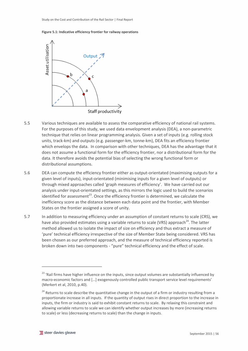
Study on the Cost and Contribution of the Rail Sector | Final Report
September 2015 | 56
Figure 5.1: Indicative efficiency frontier for railway operations
5.5 Various techniques are available to assess the comparative efficiency of national rail systems.
For the purposes of this study, we used data envelopment analysis (DEA), a non-parametric
technique that relies on linear programming analysis. Given a set of inputs (e.g. rolling stock
units, track-km) and outputs (e.g. passenger-km, tonne-km), DEA fits an efficiency frontier
which envelops the data. In comparison with other techniques, DEA has the advantage that it
does not assume a functional form for the efficiency frontier, nor a distributional form for the
data. It therefore avoids the potential bias of selecting the wrong functional form or
distributional assumptions.
5.6 DEA can compute the efficiency frontier either as output-orientated (maximising outputs for a
given level of inputs), input-orientated (minimising inputs for a given level of outputs) or
through mixed approaches called ‘graph measures of efficiency’. We have carried out our
analysis under input-orientated settings, as this mirrors the logic used to build the scenarios
identified for assessment23. Once the efficiency frontier is determined, we calculate the
inefficiency score as the distance between each data point and the frontier, with Member
States on the frontier assigned a score of unity.
5.7 In addition to measuring efficiency under an assumption of constant returns to scale (CRS), we
have also provided estimates using a variable returns to scale (VRS) approach24. The latter
method allowed us to isolate the impact of size on efficiency and thus extract a measure of
‘pure’ technical efficiency irrespective of the size of Member State being considered. VRS has
been chosen as our preferred approach, and the measure of technical efficiency reported is
broken down into two components - “pure” technical efficiency and the effect of scale.
23 ‘Rail firms have higher influence on the inputs, since output volumes are substantially influenced by
macro-economic factors and […] exogenously controlled public transport service level requirements’ (Merkert et al, 2010, p.40).
24 Returns to scale describe the quantitative change in the output of a firm or industry resulting from a
proportionate increase in all inputs. If the quantity of output rises in direct proportion to the increase in inputs, the firm or industry is said to exhibit constant returns to scale. By relaxing this constraint and allowing variable returns to scale we can identify whether output increases by more (increasing returns to scale) or less (decreasing returns to scale) than the change in inputs.

Study on the Cost and Contribution of the Rail Sector | Final Report
September 2015 | 57
5.8 The clustering analysis presented in the previous chapter has also informed the DEA as
follows:
EU-wide efficiency scores are calculated using all 26 Member States within the sample;
Member States (and their efficiency scores) are grouped according to the clusters
estimated in Chapter 4; and
Efficiency scores are subsequently re-based according to the level of efficiency achieved
by the best-in-cluster Member State (a worked example is provided in paragraphs 6.4 to
6.8).
Application of data envelopment analysis
5.9 Given the flexibility of DEA to incorporate measures of inputs and outputs across multiple
dimensions, we followed a systematic but iterative approach to analyse the efficiency of
national railway systems. Table 5.1 describes the combination of inputs and outputs used in
the six DEA models on which our efficiency assessment is based. These combinations of inputs
and outputs have been chosen as they most closely reflect the KPIs described in Chapter 3 and
the scenario development activities explained in Chapter 6. A single model was then selected
to inform the scenario assessment exercise. Detailed results for the six models described in
Table 5.1 are provided in Appendix E.
Table 5.1: Selected data envelopment analysis models
Total capital productivity^
Passenger only
Freight only Track
utilisation Train
utilisation
DEA model 1 2* 3 4 5 6
Outputs Passenger km
Tonne km
Inputs
Track km
Rolling stock (passenger)
Rolling stock (freight)
^ Total capital productivity is defined as including both track and train (freight and passenger) related inputs simultaneously within the data envelopment model
* Model 2 is identical to model 1 except that it captures three years of data rather than one (2012)
Results
5.10 The remainder of this chapter summarises the results from the data envelopment models
described in Table 5.1 with greater focus on the ‘total capital productivity’, ‘track utilisation’
and ‘train utilisation’ results as these most directly correspond to the levers available to the
Commission to influence rail efficiency across Europe. Detailed results from the data
envelopment analysis are provided in Appendix E.
5.11 It should be noted that, when reporting the results of the DEA, we have used the convention
that the term ‘productivity coefficient’ describes the efficiency scores generated when
assuming constant returns to scale. We use the term ‘technical efficiency coefficient’ to
represent efficiency scores when assuming variable returns to scale, which is now measured
separately from the ‘scale effect’ that takes into account the size of the rail system across
Member States. By definition, the productivity coefficient is the product of the technical
efficiency coefficient and the scale coefficient.

Study on the Cost and Contribution of the Rail Sector | Final Report
September 2015 | 58
Total capital productivity
5.12 We developed two DEA models to explore the characteristics of total capital productivity
(defined as including both track, freight train and passenger train related inputs
simultaneously within a single data envelopment model). The first was a static model which
only took account of the relative performance of Member States in 2012. The rationale behind
this model was to understand how well Member States are able to combine both track
infrastructure and rolling stock assets to deliver both passenger and freight outputs. Under an
assumption of variable returns to scale, half of the Member States included were considered
to be on the efficiency frontier. This is a function of the large number of both inputs and
outputs that are included within the analysis and the fact that individual observations are
therefore more likely to be captured by the efficiency frontier (which is expressed in a large
number of dimensions). As can be seen in Figure 5.2, with the exception of Poland, Member
States in cluster C appear to perform particularly poorly against this specification of inputs and
outputs.
Figure 5.2: Total capital productivity technical efficiency scores (DEA model 1 VRS) - 2012 (not re-based)
Source: SDG analysis
5.13 A second DEA model was developed using identical input and output measures, but which
included observations from 2010 to 2012, chain-linked using a Malmquist Index25. The
purpose of this test was to examine the stability of technical efficiency coefficients through
time. In-line with a number of modelled but un-reported DEA assessments (considering both
three and six-year time horizons), the results of this model showed that coefficients were
25 The Malmquist Index (MI) is a bilateral index that can be used to compare the production technology
of two economies. It is also called the Malmquist Productivity Index and is based on the concept of the
production function.
0.00
0.10
0.20
0.30
0.40
0.50
0.60
0.70
0.80
0.90
1.00
BE DK IE LU NL AT FI DE ES FR IT SE UK BG CZ HU PL RO EE EL HR LV LT PT SI SK
Cluster A Cluster B Cluster C Cluster D
Tech
nic
al e
ffic
ien
cy c
oe
ffic
ien
t

Study on the Cost and Contribution of the Rail Sector | Final Report
September 2015 | 59
largely static through time and could not be used to discern efficiency trajectories. Further
details can be found in Appendix E.
Passenger efficiency
5.14 We examined passenger efficiency by limiting the input measures used to track kilometres and
passenger rolling stock, and the output measures to passenger kilometres. While the results
are broadly as expected, with primarily higher-income western European Member States
dominating the efficiency frontier, the presence of Estonia on the frontier was surprising (see
Figure 5.3. Upon inspection of the results generated under an assumption of constant returns
to scale, we observed that Estonia is the least efficient Member State. It is likely, therefore,
that the very small size of the Estonian passenger network (delivering just 235m passenger
kilometres in 2012) means that scale effects are having a significant (and potentially spurious)
impact upon the technical efficiency score for the country under an assumption of variable
returns to scale.
Figure 5.3: Technical efficiency scores for passenger rail (DEA model 3 VRS) – 2012 (not re-based)
Source: SDG analysis
Freight efficiency
5.15 The freight efficiency model is a direct parallel to the passenger efficiency model in that the
inputs are track kilometres and freight wagons, and the only output is tonne kilometres. As
shown in Figure 5.4, the best performing Member States are all relatively small, Northern
European countries and, given the dominance of Russian transit freight it is unsurprising to see
two Baltic States represented. There is no discernible trend in freight technical efficiency by
cluster, although Member States in clusters B and C perform less well than those in clusters A
and D.
0.00
0.10
0.20
0.30
0.40
0.50
0.60
0.70
0.80
0.90
1.00
BE DK IE LU NL AT FI DE ES FR IT SE UK BG CZ HU PL RO EE EL HR LV LT PT SI SK
Cluster A Cluster B Cluster C Cluster D
Tech
nic
al e
ffic
ien
cy c
oe
ffic
ien
t

Study on the Cost and Contribution of the Rail Sector | Final Report
September 2015 | 60
Figure 5.4: Technical efficiency scores for rail freight (DEA model 4 VRS) – 2012 (not re-based)
Source: SDG analysis
Track utilisation
5.16 Figure 5.5 shows that five of the six Member States on the efficient frontier generated by this
model are higher-income western European countries, all of which procure a large proportion
of their passenger services through public service contracts (this proportion is lower in
Luxembourg due to the importance of international services). It is, therefore, unsurprising
that they demonstrate high levels of track utilisation. The presence of Latvia on the efficient
frontier is notable since we might expect this to be a result of the scaling process when
considering variable returns to scale. However, under constant returns to scale both Latvia
and the Netherlands are on the efficient frontier.
5.17 This result is highly likely to be the result of the intensity with which freight traffic uses the rail
network in Latvia. Despite having the third most disperse network in the European Union
(measured by rail network length per capita), the Latvian rail network conveys more than
double the quantity of freight per capita than its nearest rival Lithuania, and twenty times that
of France.
0.00
0.10
0.20
0.30
0.40
0.50
0.60
0.70
0.80
0.90
1.00
BE DK IE LU NL AT FI DE ES FR IT SE UK BG CZ HU PL RO EE EL HR LV LT PT SI SK
Cluster A Cluster B Cluster C Cluster D
Tech
nic
al e
ffic
ien
cy c
oe
ffic
ien
t
Study on the Cost and Contribution of the Rail Sector | Final Report
September 2015 | 61
Figure 5.5: Track utilisation technical efficiency scores (DEA model 5 VRS) – 2012 (not re-based)
Source: SDG analysis
Train utilisation
5.18 As can be seen in Figure 5.6, it is notable that a very large number of Member States are on
the efficiency frontier in the train utilisation model. In the case of some Member States, this is
because the variable returns to scale assumption identifies the cost minimising size of rail
systems and then limits the comparison between Member States to those within a similar
distance from the optimum. In contrast to many of the other models, however, in this case
many large Member States are perceived to be operating at a level of output beyond the cost
efficient level and therefore exhibit decreasing returns to scale. If their operations were
smaller, i.e. they delivered fewer train kilometres, they would be able to operate more
efficiently. Under an assumption of constant returns to scale, only smaller Member States
(Denmark, Sweden, Netherlands, Latvia and Lithuania) can be found on the efficient frontier.
5.19 This result suggests that further work to investigate the optimal size of rail networks may
provide insights on the mechanisms and policy levers through which greater efficiency can be
achieved. In the presence of diseconomies of scale there may be a case for horizontal and/or
vertical separation. It is notable, however, that the UK rail network in aggregate exhibits
diseconomies of scale despite considerable horizontal separation. The observed outcome
may, therefore, be a feature of co-ordination failure, coupled with extensive public service
obligations that require the provision of services on sparsely utilised sections of the network.
0.00
0.10
0.20
0.30
0.40
0.50
0.60
0.70
0.80
0.90
1.00
BE DK IE LU NL AT FI DE ES FR IT SE UK BG CZ HU PL RO EE EL HR LV LT PT SI SK
Cluster A Cluster B Cluster C Cluster D
Tech
nic
al e
ffic
ien
cy c
oe
ffic
ien
t

Study on the Cost and Contribution of the Rail Sector | Final Report
September 2015 | 62
Figure 5.6: Train utilisation technical efficiency scores (DEA model 6 VRS) – 2012 (not re-based)
Source: SDG analysis
Conclusions
5.20 The findings of the data envelopment analysis have extended our understanding of the
performance measures obtained through the analysis of KPIs. They provide an estimate of the
efficiency gap between best and worst performing Member States (both across the entire
dataset and within clusters) across a range of scenarios. As discussed further in Chapter 6, the
‘total capital productivity’ model discussed here will be used to define the core scenario used
in the scenario assessment exercise. They also support the rationale for selecting those
Member States that are used to estimate output and employment multipliers. Further details
are provided in the following chapter.
0.00
0.10
0.20
0.30
0.40
0.50
0.60
0.70
0.80
0.90
1.00
BE DK IE LU NL AT FI DE ES FR IT SE UK BG CZ HU PL RO EE EL HR LV LT PT SI SK
Cluster A Cluster B Cluster C Cluster D
Tech
nic
al e
ffic
ien
cy c
oe
ffic
ien
t
Study on the Cost and Contribution of the Rail Sector | Final Report
September 2015 | 63
6 Scenario assessment 6.1 This chapter describes our approach to scenario definition and assessment. A single core
scenario has been defined, and an assessment made of the direct and indirect impacts of a
'best performing' rail system upon the wider economy. In addition to economic impacts (e.g.
GDP and employment impacts), we have estimated the impacts in terms of transport system
externalities (emissions, noise and safety).
6.2 In this chapter, we describe the core scenario, the steps taken to quantify its impacts and the
results obtained. We also set out the methodology used to estimate output and employment
multipliers, which capture the upstream impacts of changes to rail industry outputs on the
wider economy. Finally, we describe the results of an additional, supplementary scenario,
based upon assumptions about the impact of a change in the relative cost of road and rail
travel.
Scenario definition
6.3 After consideration of the range of policy levers available to the Commission that can be used
to support improvements to the efficiency of the EU rail sector, we focused on scenarios which
captured measures of capital productivity rather than staff or total factor productivity. We
therefore considered the following three scenarios:
Total capital productivity: considers how Member States combine all capital inputs (both
track and train) to deliver rail outputs (passenger km and tonne km);
Track utilisation: considers how Member States can, in isolation, optimise the number of
trains running on their network to improve track utilisation and hence deliver rail outputs
more efficiently; and
Train utilisation: considers how Member States can, in isolation, optimise load factors on
freight and passenger trains in order to deliver rail outputs more efficiently.
6.4 To reflect the trade-offs available to Member States when planning and delivering rail services
we decided to take forward the total capital productivity option as our core scenario. The
basic premise of the core scenario is that all Member States currently operating away from the
efficient frontier move, over a period of time, towards the frontier. In doing so, however, they
are constrained such that they cannot exceed the current performance of the most-efficient
Member State within the same cluster.
6.5 Table 6.1 provides a stylised example of this process for five Member States (1 to 5) and two
clusters (A and B). The left-hand panel represents the efficiency scores directly generated by
the DEA using the full sample of Member States. Member State 1 is the best in class (and best
in cluster A), and Member State 3 is the best in cluster B.
6.6 The middle panel shows the results of the rebasing exercise. In cluster A the efficiency scores
are unchanged since Member State 1 is on the efficiency frontier and therefore other Member

Study on the Cost and Contribution of the Rail Sector | Final Report
September 2015 | 64
States in the cluster are expected to be able to reach this level of efficiency. In cluster B,
however, the best-in-cluster Member State is not on the efficiency frontier. We assume that
other Member States in cluster B will not be able to exceed the performance of the best-in-
cluster Member State, and therefore the efficiency scores are re-based accordingly (e.g. the
rebased efficiency score for Member State 4 is 0.40 ÷ 0.80 = 0.50 where 0.80 is the efficiency
score of the best-in-cluster).
6.7 Finally, as shown in the right-hand panel, it is possible to express the efficiency scores as an
‘efficiency gap’ that describes the reduction in inputs that could be achieved while maintaining
the same level of outputs for a given Member State. A score of 0% indicates that the Member
State is performing as well as the best in cluster.
Table 6.1: Using clusters to re-base DEA outputs
DEA outputs
Re-based DEA outputs
Re-based efficiency gap
Member State
Cluster Efficiency
Score Member
State Cluster
Re-based Efficiency
Score
Member State
Cluster Efficiency
Gap
1 A 1.00 1 A 1.00 1 A 0%
2 A 0.80 2 A 0.80 2 A 20%
3 B 0.80 3 B 1.00 3 B 0%
4 B 0.40 4 B 0.50 4 B 50%
5 B 0.60 5 B 0.75 5 B 25%
6.8 The purpose of this approach is two-fold. First, controlling for the influence of exogenous
factors outside the efficiency analysis allows us to use the full sample within the estimation
process. Second, limiting the size of the efficiency gap is a prudent assumption. It means that
less efficient Member States are only expected to catch-up with their peers, rather than with
the very best performing railways across the EU.
6.9 This approach requires us to adopt the following assumptions:
The best-performing railways in Europe are on the efficient frontier. While there may be
rail systems outside the EU that are more efficient, these are unobserved and it is not,
therefore, possible to estimate any residual technical efficiency gap.
The efficiency savings gained are, and can be directly translated into, additional railway
outputs e.g. passenger kilometres or freight tonne kilometres. In practice, there may be a
range of constraints, particularly network capacity and households’ propensity to travel by
rail, which may limit expansion in rail output that is possible and/or desirable.
6.10 In addition, the scope of the analysis has certain limitations:
The analysis considers only efficiency gains related to the utilisation of physical assets and
ignores differences in unit costs. Therefore Member States already on the efficiency
frontier (measured in terms of their asset utilisation rate) could, potentially, still improve
their cost efficiency in line with that of the best performers26.
Only capital productivity is considered, leaving labour productivity out of scope.
Service quality and safety performance are not within scope.
26
For example, in Table 6.2 both France and Germany are considered to be on the efficient frontier. However, cost efficiency in Germany is demonstrably better than in France.
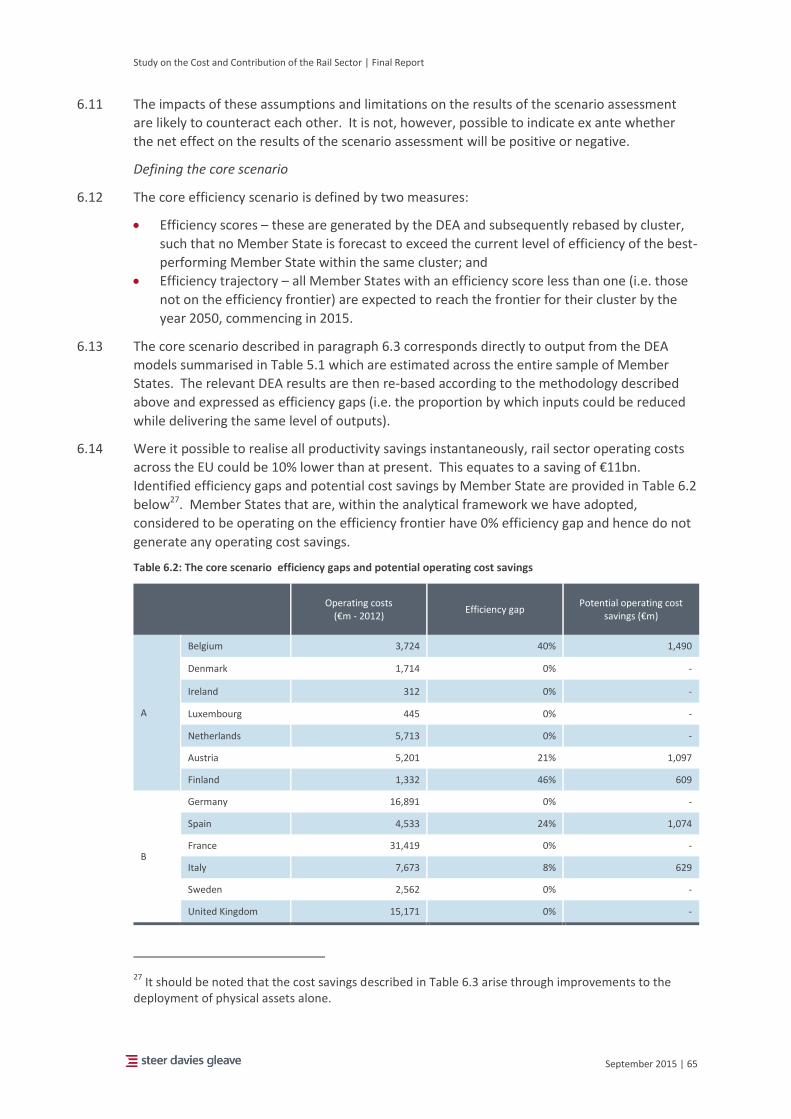
Study on the Cost and Contribution of the Rail Sector | Final Report
September 2015 | 65
6.11 The impacts of these assumptions and limitations on the results of the scenario assessment
are likely to counteract each other. It is not, however, possible to indicate ex ante whether
the net effect on the results of the scenario assessment will be positive or negative.
Defining the core scenario
6.12 The core efficiency scenario is defined by two measures:
Efficiency scores – these are generated by the DEA and subsequently rebased by cluster,
such that no Member State is forecast to exceed the current level of efficiency of the best-
performing Member State within the same cluster; and
Efficiency trajectory – all Member States with an efficiency score less than one (i.e. those
not on the efficiency frontier) are expected to reach the frontier for their cluster by the
year 2050, commencing in 2015.
6.13 The core scenario described in paragraph 6.3 corresponds directly to output from the DEA
models summarised in Table 5.1 which are estimated across the entire sample of Member
States. The relevant DEA results are then re-based according to the methodology described
above and expressed as efficiency gaps (i.e. the proportion by which inputs could be reduced
while delivering the same level of outputs).
6.14 Were it possible to realise all productivity savings instantaneously, rail sector operating costs
across the EU could be 10% lower than at present. This equates to a saving of €11bn.
Identified efficiency gaps and potential cost savings by Member State are provided in Table 6.2
below27. Member States that are, within the analytical framework we have adopted,
considered to be operating on the efficiency frontier have 0% efficiency gap and hence do not
generate any operating cost savings.
Table 6.2: The core scenario efficiency gaps and potential operating cost savings
Operating costs (€m - 2012)
Efficiency gap Potential operating cost
savings (€m)
A
Belgium 3,724 40% 1,490
Denmark 1,714 0% -
Ireland 312 0% -
Luxembourg 445 0% -
Netherlands 5,713 0% -
Austria 5,201 21% 1,097
Finland 1,332 46% 609
B
Germany 16,891 0% -
Spain 4,533 24% 1,074
France 31,419 0% -
Italy 7,673 8% 629
Sweden 2,562 0% -
United Kingdom 15,171 0% -
27 It should be noted that the cost savings described in Table 6.3 arise through improvements to the
deployment of physical assets alone.

Study on the Cost and Contribution of the Rail Sector | Final Report
September 2015 | 66
C
Bulgaria 370 75% 279
Czech Republic 2,753 68% 1,885
Hungary 1,655 58% 958
Poland 3,354 0% -
Romania 2,188 69% 1,505
D
Estonia 82 0% -
Greece 1,217 39% 478
Croatia 106 38% 40
Latvia 500 0% -
Lithuania 570 0% -
Portugal 1,038 26% 271
Slovenia 365 0% -
Slovakia 1,239 62% 771
EU26 112,128 10% 11,086
6.15 In practice, it is unrealistic to assume that rail operations can realise efficiency savings
instantaneously. Therefore, for the purposes of the core scenario assessment we have
assumed that all Member States currently operating below the efficiency frontier would follow
a linear improvement to reach the level of performance of the best-in-cluster Member State
by 2050.
6.16 There are a number of mechanisms via which potential efficiency savings can be achieved,
examples of which are provided in Chapter 7. For the purposes of this study, however,
regardless of the time-horizon or mechanism through which cost savings are achieved, we
have assumed that the savings gained are directly translated into additional railway outputs as
measured by passenger and freight tonne kilometres rather than reducing railway sector
resources.
Assessing the core scenario
6.17 The long-term impacts of efficiency improvements have been considered with reference to a
counterfactual scenario. For this study, the counterfactual scenario against which the core
‘efficiency scenario’ is compared is the European Commission Reference Scenario 2013, with
the EU-wide assessment aggregated from separate calculations for each Member State28. It is
defined in terms of:
Exogenous variables: GDP and population;
Rail Inputs: track kilometres, rolling stock, operating costs;
Transport Outputs: road passenger and freight kilometres, rail passenger and freight
kilometres; and
Externalities: road passenger and freight CO2 emissions, rail passenger and freight CO2
emissions.
6.18 Baseline data is provided at five-year intervals between 2010 and 2050, and we have applied
linear interpolation between these dates in order to generate estimates for intermediate
years.
28 http://ec.europa.eu/transport/media/publications/doc/trends-to-2050-update-2013.pdf
Study on the Cost and Contribution of the Rail Sector | Final Report
September 2015 | 67
6.19 In applying the core scenario we have:
Estimated the change in value added/operating surplus that would result if all efficiency
savings were retained;
Estimated the change in rail sector outputs (e.g. passenger kilometres) that could be
achieved if all efficiency savings were reinvested into the rail sector (using outputs from
the DEA) in order to define the comparator ‘efficiency scenario’29;
Applied output and employment multipliers (estimated according to the methodology
described in the following section) to calculate the change in direct/indirect GVA and
employment;
Applied external cost valuations from the Update of the Handbook on External Costs of
Transport (European Commission, 2014) alongside estimates of rail/road diversion factors
to calculate the welfare impacts of increased rail usage; and
Generated net present value estimates for all monetary values30.
Estimating economic impacts
Methodology
6.20 We have used a static input-output analysis framework to estimate the impact of changes in
productivity in the rail sector on the wider economy. Input-output analysis is one of a set of
related quantitative methods that represents macroeconomic activity as a system of
interrelated goods and services and shows how the parts of the system are affected by a
specific change in one particular sector (in this case a change in the efficiency of the rail
sector).
6.21 This approach requires the adoption of assumptions that are implicit in the input-output
methodology, including:
Relative prices remaining constant: the analysis assumes that the relative prices of sector
inputs remain constant;
Factor supplies meeting demand: it is assumed that the supply of factors of production
(e.g. capital) do not constrain the production of output and hence the supply of output of
a sector will increase to match demand; and
Factor proportions remaining fixed: over the time horizons defined by the scenario
assessment we might expect factor proportions to change. This suggests that,
notwithstanding the constraints identified previously, the true impact of an efficiency
improvement is likely to be larger than estimated by this study.
Creating the sectors of interest using direct employment data
6.22 The first step was to isolate the rail sector from all other sectors within the input-output tables
as these only report outputs from the rail sector at a high level of industrial disaggregation
(NACE Rev.2). The transport of passengers and freight by rail is contained within the ‘land
29 By using variable returns to scale assumptions the data envelopment analysis accounts for size in
determining the distance to the efficient frontier. As Member States re-invest efficiency savings and increase output we might, therefore, expect the scope for improvement to vary in-line with the change in scale. In practice, however, the scale of variation captured by the data envelopment analysis is far greater than the potential change in scale delivered through re-investment and the impact is expected to be marginal.
30 We have used the standard European Commission discount rate of 4%
Study on the Cost and Contribution of the Rail Sector | Final Report
September 2015 | 68
transport and transport via pipelines’ branch (49), which also includes transport by road and
the movement of freight via pipeline. The activities of the infrastructure manager are included
in ‘service activities incidental to land transportation’ (52.21).
6.23 In order to estimate the economic effects specifically for the rail sector, we have further
differentiated the original input-output tables so that the provision of passenger and freight
rail services is extracted from the rest of the sector. The goal here was to introduce a new
sector that reflected the composition of the national rail market, for which we could then
estimate indirect output and employment multipliers.
6.24 To generate the relevant sub-sectors within the input-output tables, we used structural data
(employment and GVA per worker) from individual Member States to identify the sub-sectors'
share of the higher-level sectors (e.g. share of rail transport in relation to all activities in the
‘land transport and transport via pipelines' branch)31. Following best practice, we have also
included a productivity adjustment based on average GVA per worker in the sectors of
interest. This results in different multipliers for the output and employment effects, as
presented in Table 6.3 below. In the small number of cases where GVA data at the correct
level of granularity was unavailable, or when the GVA-based results were counter-intuitive,
our approach was to use direct employment in the rail sector32.
6.25 The process for isolating the rail sector in the input-output tables was as follows:
Direct employment and GVA per worker figures for the broader sectors that make up the
rail sector were collected and the overall value added for each of the components of the
original sectors was derived (where unavailable, direct employment only was used)33;
These value added figures were then used to estimate the share of each original sector
(NACE sectors 49 and 52) to be apportioned to the new sector (rail sector);
We treated the supply, use, and compensation for employees in a proportional manner to
GVA; and
Following this apportionment, the results were consolidated into the new ‘rail sector’.
Input-output analysis
6.26 In determining the relationship between the inputs required to provide rail services and the
outputs generated by the rail sector, we used an open-static model based on national input-
output tables as inputs34.
6.27 To understand how the rail industry of individual Member States combines inputs, we have
applied a classic input-output analysis which allows the estimation of the indirect effects of
31 GVA and employment data were sourced from Eurostat, the European Annual Business Survey and
the European Union Labour Force Survey
32 This was the case for Slovakia and the Czech Republic
33 While excluding productivity-based measures from the analysis may introduce a small bias into the
isolation of the rail sector from other NACE sectors, once applied in subsequent steps to generate a weighted average employment and output multiplier for the rail sector, the impact is expected to be small.
34 An “open” model is one in which inflows and outflows caused by imports and exports within and
beyond the European Union are captured such that the multipliers estimated can capture the impact of leakages and injections. A static model is one in which factor proportions are assumed to remain fixed through time.

Study on the Cost and Contribution of the Rail Sector | Final Report
September 2015 | 69
the economic activity of a certain industry (in this case, the newly created ‘rail sector’) on
output and employment over the whole supply chain. For example, in order to provide rail
passenger services, a train operator needs inputs from other sectors such as energy,
consulting, financial services, food and beverage services etc. In turn, the energy sector will
require a range of inputs, including the extraction of crude petroleum and gas, manufacture of
coke and refined petroleum products and possibly rail freight services.
6.28 The relationship between the rail sector and the range of upstream sectors required to
generate rail services was quantified by our Leontief model. In the first stage of the analysis,
we estimated the economic effects of interrelations between the rail industry and its direct
suppliers from different sectors. We then calculated the direct supply interrelations of the
first-stage supplying sectors e.g. the energy sector35. In theory, we would have run this
process infinitely, which would result in an infinite number of calculations. A so-called
"Leontief inverse" provides a mathematical approximation of the output of the infinite
process.
6.29 Having obtained the output multipliers, we have augmented the calculation of the Leontief
inverse multipliers with an assessment of labour intensities. Labour intensity is defined as the
relative number of employees compared to value added or production output. In some cases,
this adjustment results in a higher employment multiplier than the output multipliers. In other
cases, the opposite occurs, given the relative productivity, labour laws and historical
employment in the railway sector in different Member States.
6.30 We carried out the analysis for eight Member States, selecting two in each cluster. In each
case, we analysed both the domestic multipliers (assuming imports and exports are treated as
leakages) and total multipliers (assuming that only imports and exports to/from countries
outside the EU are treated as leakages).
6.31 The choice of Member States within a cluster upon which to carry out the input-output
analysis was primarily a function of data availability. Given that we have used a static
modelling approach in which factor proportions are assumed fixed, it was important to obtain
the most up-to-date input-output data such that the factor proportions it describes reflect
recent technological developments. At the same time, based upon the assessment of KPIs
described in Chapter 3 we sought to identify ‘typical’ Member States within each cluster and
which provided a representative split between passenger and freight outputs.
Key results
6.32 The main results of our analysis are presented in Table 6.3, Figure 6.1 and Figure 6.2.
Table 6.3: Rail sector output and employment multipliers (indirect) for a sample of Member States
Cluster Member State Output multiplier Employment multiplier
Domestic SIOT Total SIOT Domestic SIOT Total SIOT
A Austria 1.90 2.36 1.88 2.23
Netherlands 1.55 1.90 1.38 1.54
B Italy 2.30 2.72 2.76 3.30
UK 1.98 2.35 2.50 2.99
35 The ‘energy’ sector is captured within the NACE2 classification as electricity, gas, steam and air
conditioning supply.
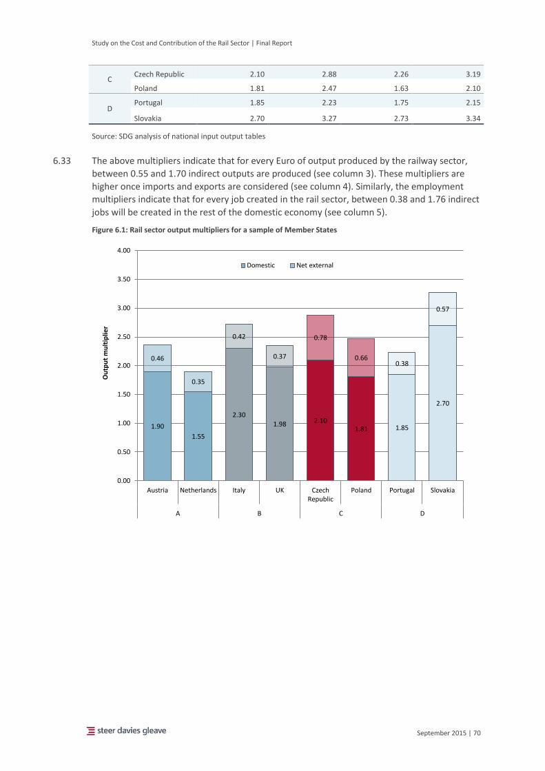
Study on the Cost and Contribution of the Rail Sector | Final Report
September 2015 | 70
C Czech Republic 2.10 2.88 2.26 3.19
Poland 1.81 2.47 1.63 2.10
D Portugal 1.85 2.23 1.75 2.15
Slovakia 2.70 3.27 2.73 3.34
Source: SDG analysis of national input output tables
6.33 The above multipliers indicate that for every Euro of output produced by the railway sector,
between 0.55 and 1.70 indirect outputs are produced (see column 3). These multipliers are
higher once imports and exports are considered (see column 4). Similarly, the employment
multipliers indicate that for every job created in the rail sector, between 0.38 and 1.76 indirect
jobs will be created in the rest of the domestic economy (see column 5).
Figure 6.1: Rail sector output multipliers for a sample of Member States
1.90
1.55
2.30
1.98 2.10 1.81 1.85
2.70
0.46
0.35
0.42
0.37
0.78
0.66 0.38
0.57
0.00
0.50
1.00
1.50
2.00
2.50
3.00
3.50
4.00
Austria Netherlands Italy UK CzechRepublic
Poland Portugal Slovakia
A B C D
Ou
tpu
t m
ult
iplie
r
Domestic Net external
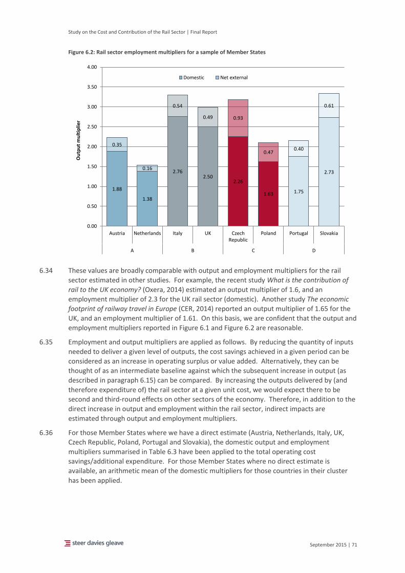
Study on the Cost and Contribution of the Rail Sector | Final Report
September 2015 | 71
Figure 6.2: Rail sector employment multipliers for a sample of Member States
6.34 These values are broadly comparable with output and employment multipliers for the rail
sector estimated in other studies. For example, the recent study What is the contribution of
rail to the UK economy? (Oxera, 2014) estimated an output multiplier of 1.6, and an
employment multiplier of 2.3 for the UK rail sector (domestic). Another study The economic
footprint of railway travel in Europe (CER, 2014) reported an output multiplier of 1.65 for the
UK, and an employment multiplier of 1.61. On this basis, we are confident that the output and
employment multipliers reported in Figure 6.1 and Figure 6.2 are reasonable.
6.35 Employment and output multipliers are applied as follows. By reducing the quantity of inputs
needed to deliver a given level of outputs, the cost savings achieved in a given period can be
considered as an increase in operating surplus or value added. Alternatively, they can be
thought of as an intermediate baseline against which the subsequent increase in output (as
described in paragraph 6.15) can be compared. By increasing the outputs delivered by (and
therefore expenditure of) the rail sector at a given unit cost, we would expect there to be
second and third-round effects on other sectors of the economy. Therefore, in addition to the
direct increase in output and employment within the rail sector, indirect impacts are
estimated through output and employment multipliers.
6.36 For those Member States where we have a direct estimate (Austria, Netherlands, Italy, UK,
Czech Republic, Poland, Portugal and Slovakia), the domestic output and employment
multipliers summarised in Table 6.3 have been applied to the total operating cost
savings/additional expenditure. For those Member States where no direct estimate is
available, an arithmetic mean of the domestic multipliers for those countries in their cluster
has been applied.
1.88
1.38
2.76 2.50
2.26
1.63 1.75
2.73
0.35
0.16
0.54
0.49 0.93
0.47 0.40
0.61
0.00
0.50
1.00
1.50
2.00
2.50
3.00
3.50
4.00
Austria Netherlands Italy UK CzechRepublic
Poland Portugal Slovakia
A B C D
Ou
tpu
t m
ult
iplie
r Domestic Net external

Study on the Cost and Contribution of the Rail Sector | Final Report
September 2015 | 72
Core scenario
Overview
6.37 Having estimated output and employment multipliers as described above, and following the
methodology summarised in paragraph 6.19 we have estimated the long-term impacts of the
efficiency improvements identified by building a Calculator that combines the various
analytical streams reported above. Impacts are estimated with respect to the EU Reference
Scenario 2013. We have anchored the development of all other variables (e.g. operating cost)
to this reference scenario.
6.38 The three main impacts estimated from the Calculator for the core scenario are:
Direct and indirect GVA impacts, resulting from the direct efficiency savings following an
operational improvement. These savings are subsequently reinvested, generating indirect
GVA impacts throughout the economy based on the Input-Output multipliers;
Direct and indirect employment impacts - we estimate a number of direct jobs as the
equivalent number of FTEs (full time equivalents) that would be needed to deliver the
GVA impacts calculated above, and then estimate indirect jobs based on the input-output
multipliers; and
External benefits, resulting from modal shift from road to rail, given an assumption about
diversion of passenger and tonne-km (emissions, noise and safety/accidents).
Results
6.39 The Net Present Value (NPV) of impacts resulting from the core scenario for the EU26 is €32
billion of direct GVA, €31 billion of indirect GVA and €75 million of external benefits, for the
period 2015-2030. Figure 6.3 shows the GVA results by cluster. Cluster C has the highest direct
impacts, driven by the potential efficiency savings materialising in Bulgarian, Czech, Hungarian
and Romanian railway systems. The direct impacts in clusters B and D are smaller, but the
indirect GVA is expected to be proportionately larger given the size of the rail multipliers
identified in these economies.
6.40 Figure 6.4 shows the resulting effects on job creation. The increase in rail activity resulting
from reinvesting the operating surpluses is expected to generate 1,600 jobs across the EU, the
greatest share of which are in cluster C. These will give rise to a broadly equivalent number of
indirect jobs over the period 2015-2030. These numbers are relatively small as the focus of our
analysis is on capital productivity improvements. Should efficiency estimates be derived based
on a more balanced distribution of capital and labour impacts, the employment effects could
be greater.
6.41 External benefits are estimated to have an NPV of €75 million. The magnitude of the external
benefit estimates is a function of the assumption that all additional railway outputs that are
provided as a consequence of reinvestment of cost savings are met with an equivalent
increase in demand for passenger and rail freight. In line with standard practice, we assume
that approximately 20% of all new rail traffic is abstracted from private car or road freight
traffic, thus reducing external costs for travel by road36.
36 The external benefit for cluster B is estimated to be negative because the dis-benefit of additional
emissions, noise and accidents exceeds the benefits from the reduction in these external impacts from the assumed reduction in road use. Since all of the Member States within cluster B are large, higher-

Study on the Cost and Contribution of the Rail Sector | Final Report
September 2015 | 73
Figure 6.3: NPV of GVA impacts 2015-2030 (core scenario)
Steer Davies Gleave analysis
Figure 6.4: Estimate of employment impacts 2015-2030 (core scenario)
income countries they will have higher values for the reduction of externalities compared to other clusters, which exacerbates the scale of the negative impact.
32,263 31,401
9,445 6,847 5,945 6,777
15,109 14,429
5,452 6,951
-
5,000
10,000
15,000
20,000
25,000
30,000
35,000
Direct GVA (€ million)
Indirect GVA (€ million)
Direct GVA (€ million)
Indirect GVA (€ million)
Direct GVA (€ million)
Indirect GVA (€ million)
Direct GVA (€ million)
Indirect GVA (€ million)
Direct GVA (€ million)
Indirect GVA (€ million)
A B C D
EU26 EU26 Cluster A Cluster B Cluster C Cluster D
Ne
t p
rese
nt
valu
e 2
03
0 (
€ m
illio
n, 2
01
0 p
rice
s)
1,627 1,621
193 122 104 169
1,083 1,024
247 307
-
200
400
600
800
1,000
1,200
1,400
1,600
1,800
Dir
ect
em
plo
ymen
t
Ind
ire
ct e
mp
loym
ent
Dir
ect
em
plo
ymen
t
Ind
ire
ct e
mp
loym
ent
Dir
ect
em
plo
ymen
t
Ind
ire
ct e
mp
loym
ent
Dir
ect
em
plo
ymen
t
Ind
ire
ct e
mp
loym
ent
Dir
ect
em
plo
ymen
t
Ind
ire
ct e
mp
loym
ent
A B C D
EU26 EU26 Cluster A Cluster B Cluster C Cluster D
Ad
dit
ion
al jo
bs
stim
ula
ted
20
15
-20
30
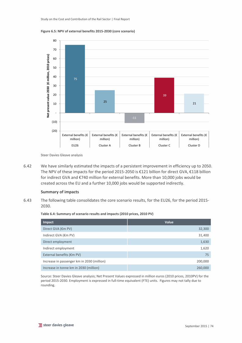
Study on the Cost and Contribution of the Rail Sector | Final Report
September 2015 | 74
Figure 6.5: NPV of external benefits 2015-2030 (core scenario)
Steer Davies Gleave analysis
6.42 We have similarly estimated the impacts of a persistent improvement in efficiency up to 2050.
The NPV of these impacts for the period 2015-2050 is €121 billion for direct GVA, €118 billion
for indirect GVA and €740 million for external benefits. More than 10,000 jobs would be
created across the EU and a further 10,000 jobs would be supported indirectly.
Summary of impacts
6.43 The following table consolidates the core scenario results, for the EU26, for the period 2015-
2030.
Table 6.4: Summary of scenario results and impacts (2010 prices, 2010 PV)
Impact Value
Direct GVA (€m PV) 32,300
Indirect GVA (€m PV) 31,400
Direct employment 1,630
Indirect employment 1,620
External benefits (€m PV) 75
Increase in passenger km in 2030 (million) 200,000
Increase in tonne km in 2030 (million) 260,000
Source: Steer Davies Gleave analysis; Net Present Values expressed in million euros (2010 prices, 2010PV) for the period 2015-2030. Employment is expressed in full-time equivalent (FTE) units. Figures may not tally due to rounding.
75
25
-11
39
21
(20)
(10)
-
10
20
30
40
50
60
70
80
External benefits (€ million)
External benefits (€ million)
External benefits (€ million)
External benefits (€ million)
External benefits (€ million)
EU26 Cluster A Cluster B Cluster C Cluster D
Ne
t p
rese
nt
valu
e 2
03
0 (
€ m
illio
n, 2
01
0 p
rice
s)

Study on the Cost and Contribution of the Rail Sector | Final Report
September 2015 | 75
Supplementary scenario analysis
Background
6.44 The supplementary scenario analysis has been developed to assess changes in relative prices
between transport modes, given that the main model developed to capture the impacts of
productivity improvements does not include an assessment of price dynamics. To this end, we
have produced an off-model calculation that assesses the impact of a change in road costs on
modal shift and estimates the additional rail demand that would result if the price of road
transport were to increase.
Methodology
6.45 In carrying out the supplementary scenario analysis we have:
Estimated cross price elasticities between road costs and rail usage (for freight and
passenger traffic separately);
Assumed a one-off shock to motoring costs in 2015;
Calculated the knock-on impact of the shock on rail demand; and
Compared the increase in rail demand caused by the shock, with the increase in rail
supply delivered in the core scenario.
Estimating cross elasticities
6.46 First, we have reviewed the existing literature on own price elasticities for road, rail, passenger
and freight transport, focusing on the following sources:
Price sensitivity of European road freight transport – towards a better understanding of
existing results (Significance, 2010);
Transit Price Elasticities and Cross Elasticities (VTPI, 2015)37;
Understanding Transport Demands and Elasticities (VTPI, 2013);
Passenger Demand Forecasting Handbook v5.1 (ATOC, 2013);
Road Traffic Demand Elasticities (RAND Europe, 2014); and
Long Run Trends in Car Use (OECD, 2013).
6.47 Our review of the literature identified that most studies base the estimation of elasticities on
the demand response to changes in fuel prices (own price demand elasticity). Where possible
we have sought to identify long-run price elasticities which, ceteris paribus, tend to be higher
than short-run elasticities. Key conclusions from our review are as follows:
It is reasonable to assume the fuel cost own price elasticity falls within a fairly narrow
range of -0.1 to -0.5, but some trips are more elastic depending on distance and purpose.
Transit ridership elasticities (mainly from US data samples) are typically in the range -0.6
to -0.9, although this varies considerably between peak and off peak, and by distance.
There is little evidence on differences in fuel price elasticities for urban and non-urban
journeys, and we are therefore not able to remove the effect of urban journeys from our
sample.
There is some consistency in the own price elasticity of freight demand, with values in the
range -0.1 to -0.6.
37 In reviewing the literature we have isolated bus fares from wider definitions of “transit” which may
include some rail systems, light rail systems and metro systems. European evidence has been given greater weight than studies from North America.

Study on the Cost and Contribution of the Rail Sector | Final Report
September 2015 | 76
6.48 In contrast, evidence on cross-elasticity values shows they are unstable and depend heavily on
the current market share between modes. Therefore we make use of the following
relationship between own price elasticities, market share and diversion factors in order to
derive cross elasticities. This is a standard relationship between own and cross elasticities that
is true by definition and which is extensively reported within the literature (see Dodgson,
1986)38.
𝑒𝐴𝐵 = |𝑒𝐵𝐵|. (𝑉𝐵 𝑉𝐴).⁄ 𝛿𝐵𝐴
where eAB is the cross elasticity of demand for A to the price of B, eBB is B’s own price elasticity,
VB/VA is the relative volume share of B to A, and δBA is the proportion of the change in demand
for B that diverts to/from A (a ‘diversion factor’).
6.49 We have adopted the following assumptions in order to populate the formula above and
estimate the additional rail demand from a change in road costs:
The evidence from the literature review has informed our own elasticity values for road
transport (-0.3 for passengers and -0.4 for freight journeys);
Separate market shares for passenger and freight transport are derived at the Member
State level based on our database for this study;
A diversion factor is the proportion of the change in demand for a mode (as a result of
cost changes) that comes from or goes to another mode. In calculating the external
benefits of the core scenario we assumed a value of 20% (i.e. 20% of road demand would
divert to rail) and for consistency we adopt the same value in this analysis.
For the purpose of this exercise a 5% uniform increase in road transport costs is
assumed39. This might come from an increase in fuel prices, the application of tolls or an
increase in private car and truck purchase / maintenance costs40.
6.50 The resulting cross-elasticities by Member State are reported in Table 6.5 below.
Table 6.5: Road Price Cross Elasticities of Demand for Rail by Member State
Member State Road Price Cross Elasticity (Rail Passenger)
Road Price Cross Elasticity (Rail Freight)
Austria -0.39 -0.14
Belgium -0.60 -0.41
Bulgaria -1.14 -0.46
Czech Republic -0.48 -0.28
Germany -0.57 -0.22
Denmark -0.45 -0.55
Estonia -2.13 -0.06
Greece -4.01 -3.65
38 Dodgson, J. S. (1986) Benefits of Changes in Urban Public Transport Subsidies in the Major Australian
Cities. Economic Record 62, pp.224-235
39 Given the variation in existing road transport costs across Member States, the variations at Member
State level may differ.
40 Recent trends suggest that the cost of passenger transport by rail is rising compared to road
transport. Between 2005 and 2014 rail passenger prices rose by 41% (EU28 excluding Malta and Cyprus) while the cost of passenger motoring rose by 36% (Harmonised Indices of Consumer Prices – Eurostat). This suggests that the scale of price shock is reasonable and could be interpreted as a reversal of the trends observed over the past decade.
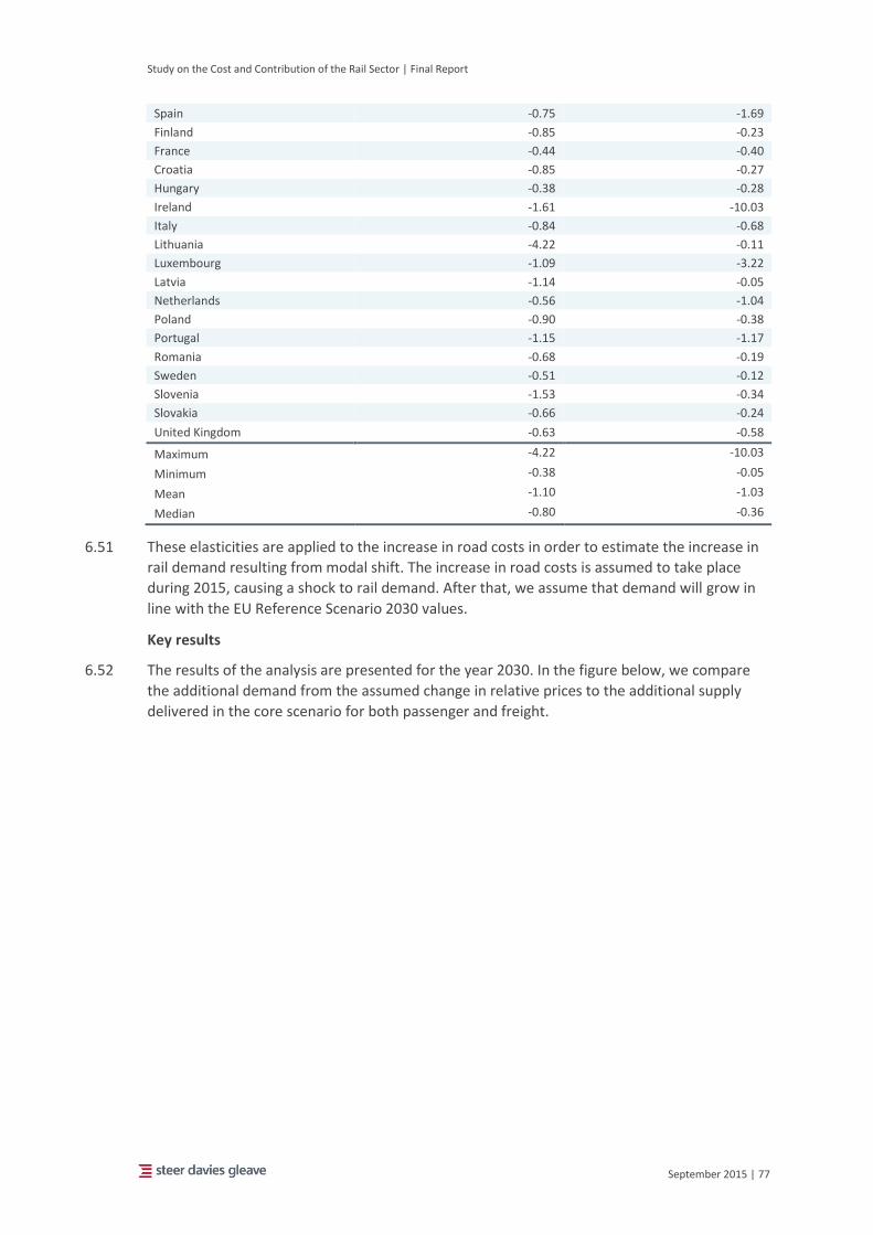
Study on the Cost and Contribution of the Rail Sector | Final Report
September 2015 | 77
Spain -0.75 -1.69
Finland -0.85 -0.23
France -0.44 -0.40
Croatia -0.85 -0.27
Hungary -0.38 -0.28
Ireland -1.61 -10.03
Italy -0.84 -0.68
Lithuania -4.22 -0.11
Luxembourg -1.09 -3.22
Latvia -1.14 -0.05
Netherlands -0.56 -1.04
Poland -0.90 -0.38
Portugal -1.15 -1.17
Romania -0.68 -0.19
Sweden -0.51 -0.12
Slovenia -1.53 -0.34
Slovakia -0.66 -0.24
United Kingdom -0.63 -0.58
Maximum -4.22 -10.03
Minimum -0.38 -0.05
Mean -1.10 -1.03
Median -0.80 -0.36
6.51 These elasticities are applied to the increase in road costs in order to estimate the increase in
rail demand resulting from modal shift. The increase in road costs is assumed to take place
during 2015, causing a shock to rail demand. After that, we assume that demand will grow in
line with the EU Reference Scenario 2030 values.
Key results
6.52 The results of the analysis are presented for the year 2030. In the figure below, we compare
the additional demand from the assumed change in relative prices to the additional supply
delivered in the core scenario for both passenger and freight.
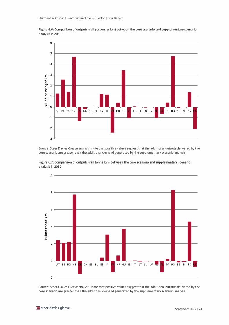
Study on the Cost and Contribution of the Rail Sector | Final Report
September 2015 | 78
Figure 6.6: Comparison of outputs (rail passenger km) between the core scenario and supplementary scenario analysis in 2030
Source: Steer Davies Gleave analysis (note that positive values suggest that the additional outputs delivered by the core scenario are greater than the additional demand generated by the supplementary scenario analysis)
Figure 6.7: Comparison of outputs (rail tonne km) between the core scenario and supplementary scenario analysis in 2030
Source: Steer Davies Gleave analysis (note that positive values suggest that the additional outputs delivered by the core scenario are greater than the additional demand generated by the supplementary scenario analysis)
-3
-2
-1
0
1
2
3
4
5
6
AT BE BG CZ DE DK EE EL ES FI FR HR HU IE IT LT LU LV NL PL PT RO SE SI SK UK
Bill
ion
pas
sen
ger
km
-2
0
2
4
6
8
10
AT BE BG CZ DE DK EE EL ES FI FR HR HU IE IT LT LU LV NL PL PT RO SE SI SK UK
Bill
ion
to
nn
e k
m

Study on the Cost and Contribution of the Rail Sector | Final Report
September 2015 | 79
6.53 The charts should be interpreted with some care. For those Member States on the efficient
frontier, the total quantity of outputs generated in 2030 by the core scenario is simply the
level projected by the EU Reference Scenario 2013 (i.e. there are no efficiency gains to be
delivered). By contrast, for those Member States currently operating away from the efficient
frontier, additional rail outputs over-and-above the EU Reference Scenario 2013 are delivered
as a result of the re-investment of cost savings achieved through efficiency improvements.
6.54 In most cases in which a Member State is currently operating inefficiently (i.e. away from the
efficient frontier), the additional demand that can be accommodated by reinvesting the
efficiency savings is broadly in line with the additional demand generated by a change in
relative prices. In practice, while some investment expenditure is likely to be required (e.g. to
upgrade junctions and signalling) our analysis suggests that the additional demand could be
served through better deployment of current rolling stock and infrastructure assets.
6.55 In other Member States, primarily where no productivity improvements have been modelled
(e.g. France), the increase in rail demand from modal shift would need to be accommodated
by further investment which, in turn, would require additional funding. Our analysis does not
attempt to quantify the exact threshold beyond which national rail systems would need extra
investment.
6.56 When results are aggregated by the Member State clusters reported in the rest of the study
we find that in all clusters except Cluster B, the additional demand generated by the motoring
cost shock is less than the additional capacity supplied in the core scenario (i.e. the additional
demand can be accommodated without further investment expenditure). However, for
Cluster B, where the potential for productivity improvements is lowest, a considerable amount
of excess demand would need to be accommodated and this might require further
investment.
6.57 At the European level, the additional rail demand resulting from a change in relative prices
would be lower than the additional demand that could be accommodated by reinvesting the
efficiency savings under the core scenario.
Table 6.6: Comparison between the supplementary scenario analysis and the core scenario by cluster
Cluster Passenger km (million) from supplementary
scenario analysis vs core scenario Tonne km (million) from supplementary
scenario analysis vs core scenario
A 2,600 6,900
B -4,600 -3,500
C 13,600 20,700
D 2,200 5,100
Steer Davies Gleave analysis. Positive figures indicate that the additional demand from the core scenario is higher than that from the core scenario.

Study on the Cost and Contribution of the Rail Sector | Final Report
September 2015 | 80
7 Policy implications The current policy context
7.1 As noted in Chapter 1, the 2011 White Paper, Roadmap to a Single European Transport Area –
Towards a competitive and resource efficient transport system, sets out a vision for the
European transport sector in which rail transport plays a much greater role than at present.
Rail’s share of both passenger and freight movements is expected to increase significantly as a
result of the generation of new traffic and a switch of existing traffic from other modes, in
particular from road. This, in turn, will require a substantial improvement in rail’s
competitiveness, delivered through a range of policy interventions covering infrastructure and
operations. The policy framework described in the White Paper is summarised in the figure
below.
Figure 7.1: The EU policy framework for the rail sector

Study on the Cost and Contribution of the Rail Sector | Final Report
September 2015 | 81
7.2 This framework includes policy interventions designed to address a number of general issues
arising across the sector with the ultimate aim to improve the quality and efficiency of rail
services. This study has demonstrated that enhancing the productivity of both the rail network
and rolling stock can deliver significant cost savings. Current EU policies, such as TEN-T and rail
freight corridors, interoperability measures and market opening aim to transition from the
patchwork of national railways to a network of EU railways, and thus enhance productivity and
cost efficiency of rail transport.
7.3 This study has nevertheless demonstrated the need to consider additional country-specific
constraints and weaknesses that are currently undermining rail industry efficiency and
competitiveness. In particular, we note that:
Some Member States, including several in Eastern Europe, have legacy networks that
were developed to serve a different profile and distribution of economic activity from that
observed today, with the result that their rail industries require substantial restructuring
and investment to realign both passenger and freight services with current economic
needs;
Others, primarily among the EU 15, have already undertaken substantial investment in
new infrastructure and rolling stock, but their networks continue to be subject to major
capacity constraints that will need to be relieved through further enhancements; at the
same time there are countries where network utilisation rates can significantly improved;
While the majority of Member States experience relatively low levels of passenger train
utilisation, often reflecting inflexible capacity and service frequency requirements in
public service contracts, some still achieve significantly higher average load factors than
others; and
Some Member States have been more successful than others in balancing the
performance of passenger and freight rail.
7.4 In addition, although there is a general concern about the overall financial sustainability of the
sector across Europe, financial constraints have taken different forms in different countries.
For example, in Bulgaria the industry’s financial position deteriorated to the point where it
could no longer cover operational expenditure, prompting the introduction of a major reform
programme supported by the World Bank in 2011. By contrast, in the UK, the financing of
operations has been on a stable footing for some years, with premiums paid by some
passenger franchisees now broadly balancing the subsidies paid to others, but some industry
commentators have nevertheless suggested that Network Rail’s ongoing accumulation of debt
to fund enhancements will prove unsustainable in the long-run.
7.5 Against this background, the interaction between EU and national rail policy requires careful
coordination. On the one hand, it is important that necessary restructuring and network
consolidation at the national level does not undermine the further development of an EU
single market in rail services. On the other key European policy initiatives, for example
support for TEN-T projects from the Connecting Europe Facility and research funded by the
Shift2Rail Joint Undertaking, will need to be implemented in a coordinated manner with
national policy measures to improve efficiency. In the following paragraphs, we consider a
number of implications for the development of both EU and national rail policies, drawing on
the results of the analysis described in previous chapters.
The need for industry restructuring
7.6 Arguably, the most important area of policy interaction relates to industry restructuring
among Member States in Eastern Europe, in particular Bulgaria, the Czech Republic, Hungary
Study on the Cost and Contribution of the Rail Sector | Final Report
September 2015 | 82
and Romania (included in cluster C in the analysis reported in Chapter 4). The results of the
DEA reported in Chapter 5 suggest that these countries must achieve substantial
improvements in efficiency if they are to catch up with Poland, the most productive Member
State in cluster C, which, after adjusting for scale effects, has one of the most productive
railways in Europe41. Reflecting this, if all four countries were to achieve this improvement
based upon 2012 outputs and operating costs, the resulting rail sector cost savings would be
€4.4bn - €5.1bn per annum, some 23% - 41% of the total annual cost savings estimated across
the 26 Member States modelled.
7.7 Our scenario analysis is necessarily simplified for the purposes of modelling, and is not
intended to simulate precisely the effects of the restructuring programme needed to raise the
efficiency of the rail industry in each country. However, the scope for efficiency
improvements and associated cost savings indicated by our analysis are broadly in line with
the aims of the industry reform measures being implemented in Bulgaria with the support of
the World Bank. We note, for example, that the programme includes a number of measures
intended to improve the efficiency of resource use as well as others focused on securing a
more efficient scale of operations, not least:
Optimisation of business units and staff, with associated cost reductions;
Disposal of businesses that are not related to railways;
Suspension of operations on railway lines that do not have any traffic, but which incur
costs;
Appointment of qualified, competent staff and management who are accountable to
Bulgarian citizens; and
Training of railway managers and workers.
7.8 We anticipate that elements of the programme, suitably modified to take account of different
national industry characteristics, could be transferred to other countries, and note that the
new Rail Reform Authority in Romania has already been charged with managing a similar
streamlining exercise. More generally, experience in Bulgaria suggests that the
implementation of major restructuring programmes is a realistic prospect, and that the level
of improvement in efficiency assumed for the purposes of the scenario analysis, while
challenging, is considered achievable by industry stakeholders. We also note that significant
improvements in efficiency have already been achieved in countries such as the United
Kingdom, Italy, Germany, Austria and Sweden as a result of the full liberalisation of rail freight
markets and the introduction of competition, albeit more limited, in rail passenger markets.
7.9 At the same time, we consider that caution should be exercised in the development and
implementation of programmes of this kind for a number of reasons:
First, reductions in the size of the asset base (for example, as a result of a reduction in the
size of the operational infrastructure network or the national rolling stock fleet) may be
necessary to ensure better targeting of existing resources in conditions of financial
constraint. At the same time, reductions in the asset base do not always result in
proportionate cost savings. By way of illustration, closure of an existing line may result in
only limited savings in maintenance costs in the short term, since it may not be cost
effective to isolate track, signalling, electrification and communications equipment until it
41 It has to be noted however that while showing high capital productivity rates, the quality of rail
infrastructure and rail services in Poland is relatively poor
Study on the Cost and Contribution of the Rail Sector | Final Report
September 2015 | 83
has deteriorated to the point where a major intervention is needed, which may take
several years. In these circumstances, substantial reductions in costs may only be possible
in the long-run. This highlights the limitations of analysis based on physical measures of
efficiency, which can overstate the potential for cost savings, at least in the short to
medium term.
Second, reductions in the size of the network, while they may deliver both efficiency
improvements and significant cost savings, may also prove inappropriate in the long term.
In the UK, the size of the national network decreased by 40% between 1960 and 1980.
While this undoubtedly led to significant cost savings, and reflected the general decline in
rail traffic resulting from a growth in road transport over the same period, it has made it
more difficult to accommodate the substantial increase in both passenger and freight
traffic since the mid-1990s. In the event, capacity previously removed has recently been
reinstated, for example on the Cotswold and Swindon to Gloucester lines where capacity
has been increased from one track to two on each route. Elsewhere, the disposal of
railway land has further constrained the ability of the industry to respond to increasing
demand through infrastructure enhancements, since reinstatement of infrastructure
would involve costly acquisition of land and change of land use, e.g. again in the UK on the
proposed Bedford to Cambridge route.
Finally, excessive rationalisation of infrastructure capacity could discourage or even
prevent competitive entry into the rail market, whether inadvertently or by design. For
example, between 1999 and 2010 Deutsche Bahn removed capacity, preventing access to
large sections of its peripheral rail network, while at the same time increasing the density
of traffic on its core network. Consequently, the availability of paths, and therefore the
scope for market entry, was reduced.
7.10 Taken together, these considerations suggest that there is some risk that sector
rationalisation, although necessary, will not deliver all of the anticipated cost savings, and/or
that it may hinder subsequent development of the industry in terms of capacity and service
offer. This highlights a need for long term planning and coordination at EU level, reliable
information on costs, capacity provision and outputs, and careful consideration of the impact
of individual restructuring programmes.
Potential policy development
Industry reporting and monitoring
7.11 The collection and consolidation of EU rail sector data was a key part of this study, and we
have prepared a database including information on costs, inputs and outputs for all Member
States, differentiating between infrastructure management and train operation and between
freight and passenger services wherever possible. However, this exercise has highlighted
various deficiencies in the available data tending to limit the potential for analysis and hence
the information used to inform policy both at national and EU level. These deficiencies are
described in more detail in Appendix A, but here we note that they include:
presentation of consolidated accounts which often combine modes and/or markets which
may straddle Member States;
omission of individuals who work for sub-contractors or agencies from employment data,
and the lack of consistency in reporting employee data according to total staff numbers or
full-time-equivalents;
lack of clarity regarding the definition of public subsidy as stated in each operator’s
regulatory accounts, which may not include indirect public subsidy such as that provided
through capital programmes or tax relief.

Study on the Cost and Contribution of the Rail Sector | Final Report
September 2015 | 84
limited availability of net debt data, which is not widely reported in regulated accounts;
and
difficulties associated with obtaining consistent time-series data for the period 2003-2013,
during which there has been considerable market liberalisation and consolidation.
7.12 This issue could be addressed through the introduction of a more prescriptive framework for
the collection of data on infrastructure management. The Commission Implementing
Regulation on rail market monitoring, reports of regulatory bodies and railway indicators
developed by ERA are first steps in this direction42. However, following the air navigation
precedent43, the information collected would be limited to that available within the
infrastructure managers (i.e. the monopoly suppliers of network infrastructure services) and
could not be expected to include the costs and revenues of train service providers, some of
which operate in competitive markets. It is a general characteristic of liberalised markets that
commercially sensitive information of this kind is often not published (at least below a high
level of aggregation) and/or may not be prepared on a consistent basis across operators. It
follows that strengthening the framework of data collection in the way outlined above would
not resolve all of the data issues identified in the course of this study44.
Ensuring optimal rail capacity
7.13 We have noted the potential for rationalisation of rail infrastructure to have an adverse effect
on the availability of capacity, including capacity that might otherwise be used by new entrant
rail service providers, and the need to consider possible long-term rail market requirements
when undertaking major restructuring. However, while the possibility of excessive
rationalisation is a general concern, potentially applying to any programme of restructuring in
Member States across the EU, whether or no specific proposals for capacity reduction are
appropriate or not will depend on the part of the network in question and the markets that it
serves (or may serve in the future). For example, it may be possible to demonstrate that
closure of a line or a marshalling yard will effectively foreclose new entry, but it may
nevertheless be the case that:
The new entrant is not able to pay non-discriminatory access charges designed to cover
the direct costs of the infrastructure (i.e. the line is genuinely commercially unviable);
and/or
The wider benefits of the new service, including environmental benefits and other
externalities, are insufficient to cover ongoing maintenance, renewal and other costs (i.e.
there is no existing economic case for continuing to operate the infrastructure, although
such a case might be made in the future).
7.14 This demonstrates the need for case-by-case appraisal of proposals for rationalisation,
drawing on the powers of rail sector regulators and competition authorities as necessary,
42 Commission Implementing Regulation (EU) No 2015/1100 of 7 July 2015 on the reporting obligations
of the Member States in the framework of rail market monitoring
43 In the European air navigation industry national service providers are subject to detailed reporting
requirements covering both the cost information required to calculate charges and more general information relating to safety, capacity, efficiency and environmental impacts
44 In the case of data for rail freight operations, there may be parallels to the annual Rail Waybill dataset
for the United States which includes shipment data from a stratified sample of rail waybills submitted by freight operators to the Surface Transportation Board

Study on the Cost and Contribution of the Rail Sector | Final Report
September 2015 | 85
where operators or other stakeholders raise concerns. More general regulatory provisions
seeking to preserve defined levels of capacity, whether at the EU or national level, are unlikely
to ensure economically optimal outcomes in which possible future capacity needs are
balanced against more immediate potential for cost savings.
7.15 Nevertheless, given the risk that major restructuring programmes designed to achieve
substantial cost savings can lead to excessive rationalisation, it is important to ensure that
stakeholders (including relevant transport authorities, representatives of passengers and
existing and potential operators) have the opportunity to express their views on the closure of
lines, stations, freight yards and other facilities. There is therefore a general need to ensure
that Member States and infrastructure managers, when developing rail infrastructure
development strategies and business plans as foreseen in Article 8 of Directive 2012/34/EU,
would consider thoroughly future mobility needs and give an opportunity to all existing and
potential users to express their views on closure of lines.
7.16 It may therefore be appropriate to develop a framework for ensuring that stakeholders are
properly consulted on the effects of rail rationalisation, to be implemented through either
legislation or guidance. In either case, consultation procedures will need to reflect the legal,
institutional and cultural environment prevailing in individual Member States, and specific
consultations will need to be tailored according to the proposals in question. Any framework
must therefore provide for flexibility, allowing Member States to balance the need for open
and transparent consultation on the one hand with effective and timely decision-making on
the other.
Exchange of experience and good practice
7.17 Our analysis has demonstrated that rail industries across the EU vary considerably in terms of
the economic and demographic environments in which they operate, their relative stages of
development, the relative importance of different markets (e.g. passenger and freight) that
they serve and the levels of efficiency that they achieve. At the same time, the clustering
analysis in Chapter 4 and the DEA in Chapter 5 have highlighted important similarities between
national rail industries within individual clusters. Against this background, we consider that
the exchange of experience and good practice, including in relation to management and
operational practice as well as policy implementation, is likely to yield significant benefits.
7.18 To some degree, this kind of exchange of information is already supported through existing
institutional arrangements, for example the framework for developing Technical Specifications
for Interoperability (TSIs) overseen by the European Railway Agency, and the work of several
pan-European rail organisations. Recently new structures have been created, such as the
European Network of Rail Regulatory Bodies (ENRRB), the Platform of Rail Infrastructure
Managers in Europe (PRIME) and Rail Undertakings' Dialogue. These forums shall continue to
encourage the dissemination of good practice in areas such as forecasting future capacity
needs and management of network rationalisation, driving productivity improvements,
opening markets, industry consultation, application of the results of new research (including
those arising from the work of Shift2Rail).
Recommendations for further work
7.19 In light of the experience gained in completing this study, it is clear that there is considerable
scope to better understand the relative efficiency of rail systems across Europe. While any
further analysis is likely to face similar data constraints to those identified in this report, we
have highlighted three areas which we consider to be promising areas for further work. They
include work to:

Study on the Cost and Contribution of the Rail Sector | Final Report
September 2015 | 86
Investigate scale effects to understand the optimal size of rail networks and agents;
Explore trade-offs between factors of production (including labour) simultaneously; and
In addition to assessment at national level, consider European rail efficiency within a
wider geographic and temporal context.
Economies of scale
7.20 The results of the data envelopment analysis described in Chapter 5 suggest that further work
to investigate the optimal size of rail networks may provide insights on the mechanisms and
policy levers through which greater efficiency can be achieved. In the presence of
diseconomies of scale there may be a case for horizontal and/or vertical separation.
7.21 These observations are supported by Sánchez, Monsálvez and Martínez (2008) who find that
the process of vertical separation has had a positive effect on the efficiency of European
railway systems45. These gains are larger when horizontal separation has also been
completed. By contrast, no significant gains are observed in productivity or efficiency when
only operations are reformed, but the vertically integrated structure of the industry is
maintained.
7.22 Other studies, however, suggest a more mixed response to vertical separation. For example,
Growitsch and Wetzel (2009) find that vertical separation raises costs while Cantos et al (2011)
find vertical separation to be statistically insignificant46. Others such as Friebel et al (2010)
find that reforms can improve efficiency, but only where they are delivered sequentially and
not part of a package, and Mizutani and Uranashi (2013) find that the impact of vertical
separation depends upon the level of traffic density on the rail network47.
Total factor productivity
7.23 Given the range of policy levers available to the European Commission to influence and
encourage the efficiency of the rail sector, this study deliberately focused upon capital
productivity. However, either by including additional factors of production, or by
disaggregating efficiency measures according to broad categories of rail-related activities, it
may be possible to shed further light on the drivers of efficiency. Further work may include:
Exploiting disaggregate (ideally company-level) data to decompose total factor
productivity between different activities performed by railway agents e.g. provision of
locomotive power, operation of carriages and wagons, provision of permanent way and
working of traffic (see Dodgson, 2011).
Gathering data on employment within the rail sector to better understand and benchmark
labour market characteristics including working conditions, market constraints, capital-
labour substitution rates etc. For example, this could build upon AECOM (2011) which
shows that average staff costs were about 20% higher in the UK than in Germany and
45 See Sánchez, Monsálvez and Martínez, Vertical and Horizontal Separation in the European Railway
Sector: Effects on Productivity
46 See Growtisch and Wetzel, Testing for Economies of Scope in European Railways: An Efficiency
Analysis and Cantos et al, Evaluating European Railway Deregulation Using Different Approaches 47
See Friebel et al, Railroad (De)Regulation – A European Efficiency Comparison and Mizutani and Uranishi, Does Vertical Separation Reduce Cost? An Empirical Analysis of the Rail Industry in European and East Asian OECD Countries.
Study on the Cost and Contribution of the Rail Sector | Final Report
September 2015 | 87
Sweden, though about 25% less in Britain than in the Netherlands (allowing for currency
differences and PPP).
Extending the scope of analysis
7.24 The majority of the analysis presented in this report considers the relative performance of
European railway systems at a single point in time. While we attempted to explore trends in
efficiency through time, the temporal dimension of our dataset is small when compared to the
number of cross-sectional observations and therefore provides limited insights. In practice,
however, the accumulation of capital will have an impact on the technology available to the
rail sector and hence the capital-labour substitution ratio would be expected to change
through time. Understanding the evolution of performance through time would allow the
development of more sophisticated, dynamic efficiency scenarios.
7.25 In addition to furthering our understanding of efficiency trajectories through time, we
consider that there may be value in extending the sample of international benchmarks beyond
the European Union. European railways may not, necessarily, represent the best benchmarks
in all cases and across all rail-related activities. As a consequence it is implicit in the findings of
this study that those Member States currently operating on the efficiency frontier cannot
improve any further given the current technological mix. In practice, this is unlikely to be the
case.


Study on the Cost and Contribution of the Rail Sector | Final Report
September 2015 | 89
Appendices

Study on the Cost and Contribution of the Rail Sector | Final Report
A Data collection – Member State notes
A.1 In addition to the generic issues described in paragraphs to , we also encountered a
number of country specific issues and gaps in data covering the years 2007 to 2012. These are
summarised by Member State below:
Austria (AT)
The passenger revenue dataset was inflated using RMMS market size data to reflect the
fact that not all operators were captured in our study. This adjustment could not be made
to the operating cost and staffing datasets as the data reported by this Member State is
not disaggregated between the Infrastructure Manager and the operator.
Czech Republic (CZ)
No subsidy data was available for 2008 from the UIC Database. We were able to identify
data from the principal Operator’s Annual Report and Accounts for the “Settlement of
losses from passenger transportation from the State/regional budget(s) including the
grant for student fares” and for “securing railway routes”. We have assumed that these
items are a subsidy, although this assumption may not be directly comparable to the
assumption underpinning UIC data for 2007 and 2009-12.
The passenger revenue, operating cost and staffing datasets were inflated using RMMS
market size data to reflect the fact that not all operators were captured in our study.
Denmark (DK)
We were unable to account for Arriva Denmark’s incomes and expenditure, as their
accounts were not presented at a sufficiently disaggregated level. We have used RMMS
data to adjust the passenger revenues, operating costs and staffing datasets to reflect this
gap.
It should be noted that staffing figures for the Infrastructure Manager (Banedanmark)
were provided as employees and not as Full Time Equivalents. However, in one set of
accounts both figures were given and they were within 1% of each other. We therefore
believe that the total staffing figures for this Member State are accurate.
Estonia (EE)
We have been unable to obtain passenger fare income, operating cost and staffing data
for the Operator AS GoRail, which is the international operator in Estonia. We have,
however, been able to obtain data for the domestic passenger operator, the
Infrastructure Manager and the principal freight operator.
Study on the Cost and Contribution of the Rail Sector | Final Report
Please note that this data was provided to us by a third party, who undertook currency
conversion calculations themselves. It is possible that slightly different conversion rates
were used.
France (FR)
SNCF Group does not disaggregate its domestic income and costs from those incurred by
its subsidiaries (including those operating outside France). It also does not provide a clear
breakdown of its revenue between fares and subsidies/public service contracts. We have
had to make a number of assumptions to produce estimates for the breakdown of SNCF
revenues.
In particular, we have assumed that the following items are considered to be subsidies:
Public Service Orders for train operations (excludes RFF PSOs)
Operating Grants
Payments received for concession financial assets
Investment grants relating to intangible assets
Any income derived from the state for Capital expenditure has not been considered as a
subsidy.
The revenue arising from fares has had to be estimated, as SNCF does not provide a
breakdown for its revenues at a Group Level. It does, however, provide figures for fares
revenue for its divisions. In order to estimate fares revenue, we have assumed the
following:
For 2003-09: the revenues generated by SNCF in France are the sum of the revenues
generated by Voyages and Proximités minus the estimated subsidy.
For 2010-13: the revenues generated by SNCF in France are calculated by following
the same formula as set out above, then deflated by 25%. This deflationary factor
has been introduced to account for the income generated by SNCF’s overseas
interests. We chose this value as this was the difference between the figure
generated by our estimate and the (single) revenue figure provided by the RMMS.
Freight revenues are equal to the income of Géodis (SNCF’s freight division).
Income raised by SNCF Infra and Gares & Connections are considered out of scope.
Finland (FI)
No Infrastructure Manager data was available for 2007 and 2008.
It should also be noted that the principal operator’s passenger revenue has been
calculated by taking away the public subsidy to passenger services from passenger
revenue. This may not be a completely accurate representation of actual fare income.
However, we believe that it provides a reasonable estimate.
Greece (EL)
No infrastructure income data was available for 2007 and 2008.
Public subsidy data was only available for 2011-13.
Staffing figures for 2007-08 may be incomplete. However, the trend in staffing levels is
very clear (there has been a significant reduction during the period 2007-13).
Italy (IT)
Data for this Member State were sourced from a relatively large number of sources. It is
possible that not all sources will be directly comparable. However, we believe that the
totals for this Member State are generally accurate.
Study on the Cost and Contribution of the Rail Sector | Final Report
Latvia (LV)
It was not possible to disaggregate the income data for the principal operator Pasažieru
Vilciens. We were also unable to obtain staffing data for this operator.
Please note that this data was provided to us by a third party, who undertook currency
conversion calculations themselves. It is possible that slightly different conversion rates
were used.
Lithuania (LT)
No major issues have been identified.
Netherlands (NL)
We were unable to account for Arriva Netherland’s incomes and expenditure, as their
accounts are not presented at a sufficiently disaggregated level. We have used RMMS
data to adjust the passenger revenue, operating costs and staffing datasets to reflect this
gap.
Poland (PL)
It should also be noted that Passenger and Infrastructure revenue were calculated by
taking away the passenger and infrastructure portion of the public subsidy respectively.
The passenger revenue dataset was inflated using RMMS market size data to reflect the
fact that not all operators were captured in our study. This adjustment could not be made
to the operating cost and staffing datasets as the data reported by this Member State is
not disaggregated between the Infrastructure Manager and the operator. That said, it
was possible to adjust the staffing data for 2012.
Portugal (PT)
Data for the passenger operator are presented at a group level, as disaggregated figures
were not available for most of the period 2003-13. It is therefore possible that non-rail
interests have been captured in our figures.
Values for depreciation and amortisation are very different in size between CP and the
infrastructure manager REFER. We are therefore not convinced that this data is
consistent and comparable.
The passenger revenue, operating cost and staffing datasets were inflated using RMMS
market size data to reflect the fact that not all operators were captured in our study.
Romania (RO)
Data on the many smaller operators is incomplete and, for this reason, have not at all
been included in the final dataset.
It should also be noted that Passenger and Infrastructure revenue were calculated by
taking away the passenger and infrastructure portion of the public subsidy respectively.
The passenger revenue, operating cost and staffing datasets were inflated using RMMS
market size data to reflect the fact that not all operators were captured in our study.
Slovakia (SK)
The passenger revenue, operating cost and staffing datasets were inflated using RMMS
market size data to reflect the fact that not all operators were captured in our study.
Study on the Cost and Contribution of the Rail Sector | Final Report
Slovenia (SI)
No debt data was available.
As UIC International Railway Statistics are not yet available for 2013, we were unable to
access data for this year.
Spain (ES)
We were unable to obtain income data (passenger, freight and subsidy) for 2003 and
2004.
We were unable obtain employee data for 2003.
There are some further gaps in data for minor operators/infrastructure managers, but we
do not believe these have a material impact.
Debt data was only available for 2009-12.
Sweden (SE)
The data collection process for Sweden has been complicated a number of issues:
There are a large number of operators that do not report to the UIC or produce
annual accounts in a consistent format
In 2010 the rail Infrastructure Manager, Banverket, was amalgamated with a number
of other transport agencies to create the organisation Trafikverket. This organisation
(a government body) does not report its accounts on a modal basis. It has therefore
been impossible to obtain disaggregated data for infrastructure revenue, costs, debt
and staff.
The Freight operator only reported complete data to the UIC in 2009.
No market share data is available from the RMMS. This means that we are unable to
scale up our data based on the market share of the operators that we are able to
account for.
We have been able to obtain reasonably complete data for 2007-08 and 2012. This may
enable some analysis, but not over the timeline covered by this study.
United Kingdom (UK)
All financial data for regulatory accounts are presented by UK Financial Year (April 1st to
March 31st) and not by calendar year. We have converted this data into Calendar Years by
calculating a weighted average of each consecutive pair of years.
Staffing data comes from multiple sources, which may not be directly comparable.
In one year (2010) it was necessary to interpolate 2009 and 2011 data to provide an
estimate for operator employees in this year.
Revenues and public subsidies for Northern Ireland railways are included, whereas
operating costs for Northern Ireland Railways (which were not provided by DRDNI) are not
included. We estimate that Northern Ireland Railways accounts for less than 1% of the
total operating costs for the UK rail sector, and so this omission is unlikely to undermine
the total figure.
Total public subsidy is provided by the Office for Road and Rail (ORR). We have been able
to identify the proportion of this subsidy that is paid to the Infrastructure Manager
(Network Rail) and franchised operators; however, we have not been able to identify
which organisations receive the remaining public funding. For the purposes of this study,
we are only presenting the total public subsidy provided by the ORR and the Department
for Regional Development in Northern Ireland (DRDNI).
Study on the Cost and Contribution of the Rail Sector | Final Report
Operating cost data for UK train operators is available via the ORR data portal but the data
series commences in 2008. We were, however, able to locate a benchmarking study,
published by ORR in 2012, that included data for the revenues and costs of franchised
train operators covering the period 2003 to 2008. This data was presented in 2010/11
prices, and therefore have been adjusted (by applying a ratio determined by comparing
ORR nominal revenue data with the revenue data provided in this study) in order to
provide an estimate for operating costs over the 2003 to 2008 period.
Study on the Cost and Contribution of the Rail Sector | Final Report
B Data tables B.1 The data tables presented in this Appendix report:
High-level indicators for each Member State over the period 2007-2012 (Tables B.1 to B.9)
Primary KPIs over the period 2007-2012 (Tables B.10 to B.12)
Primary and secondary KPIs for 2012 (Table B.13)

Study on the Cost and Contribution of the Rail Sector | Final Report
Table B.1: Freight Rolling Stock by Member State (2007 = 100)
2007 2008 2009 2010 2011 2012
Belgium 100.0 100.8 81.5 73.8 73.8 73.8
Bulgaria 100.0 103.3 95.1 94.6 132.5 133.5
Czech Republic 100.0 98.5 74.4 57.5 57.3 56.8
Denmark 100.0 100.0 100.0 100.0 99.8 99.7
Germany 100.0 118.8 121.6 116.3 118.8 116.1
Estonia 100.0 100.0 93.1 89.5 90.0 90.4
Ireland 100.0 100.0 78.8 56.3 56.3 56.3
Greece 100.0 133.5 133.5 88.5 88.5 88.5
Spain 100.0 96.5 80.2 92.4 88.5 91.1
France 100.0 102.0 93.9 99.4 95.7 92.2
Croatia 100.0 97.8 98.0 98.4 89.4 89.4
Italy 100.0 98.4 73.1 73.1 68.7 53.4
Cyprus n/a n/a n/a n/a n/a n/a
Latvia 100.0 99.5 115.0 114.9 116.6 120.2
Lithuania 100.0 101.7 100.8 97.4 97.1 96.1
Luxembourg 100.0 108.8 110.5 110.5 110.5 110.5
Hungary 100.0 100.4 99.8 99.8 99.8 99.8
Malta n/a n/a n/a n/a n/a n/a
Netherlands 100.0 107.2 114.4 121.6 128.8 136.0
Austria 100.0 165.2 147.0 154.8 94.3 98.0
Poland 100.0 100.6 98.3 92.1 88.0 85.5
Portugal 100.0 103.0 103.0 108.2 107.3 107.3
Romania 100.0 87.4 87.4 135.4 129.2 135.5
Slovenia 100.0 98.5 98.1 80.7 79.0 78.4
Slovakia 100.0 96.8 95.2 93.6 95.6 94.6
Finland 100.0 101.3 97.5 97.0 96.0 91.0
Sweden 100.0 99.0 93.1 95.4 94.0 92.5
United Kingdom 100.0 98.0 94.1 88.1 85.8 83.5
Note: Results are only provided if data for the entire time series is available

Study on the Cost and Contribution of the Rail Sector | Final Report
Table B.2: Passenger Rolling Stock by Member State (2007 = 100)
2007 2008 2009 2010 2011 2012
Belgium 100.0 97.7 104.2 104.2 100.5 100.5
Bulgaria 100.0 103.2 103.4 88.3 114.6 114.6
Czech Republic 100.0 99.9 99.7 98.9 97.7 96.8
Denmark 100.0 103.4 117.9 88.7 78.4 68.0
Germany 100.0 106.5 106.1 105.9 101.8 101.2
Estonia 100.0 100.0 100.0 100.0 100.0 100.0
Ireland 100.0 111.7 101.9 101.9 101.9 101.9
Greece 100.0 101.5 101.5 91.9 91.9 91.9
Spain 100.0 104.4 108.1 116.6 104.1 101.7
France 100.0 102.5 104.2 106.5 106.2 104.8
Croatia 100.0 100.2 94.7 94.7 94.0 94.0
Italy 100.0 96.6 122.6 122.5 105.6 98.7
Cyprus n/a n/a n/a n/a n/a n/a
Latvia 100.0 100.0 100.0 100.0 100.0 100.0
Lithuania 100.0 85.8 80.4 79.7 63.4 61.9
Luxembourg 100.0 97.9 97.9 112.0 109.9 109.9
Hungary 100.0 96.5 91.1 93.0 86.9 91.5
Malta n/a n/a n/a n/a n/a n/a
Netherlands 100.0 97.6 87.7 97.9 98.9 102.1
Austria 100.0 101.1 100.6 99.9 96.0 95.3
Poland 100.0 99.6 95.7 95.5 92.2 82.5
Portugal 100.0 99.2 98.4 91.0 89.9 92.5
Romania 100.0 95.7 95.7 87.7 80.1 72.5
Slovenia 100.0 97.1 96.5 95.2 95.2 95.2
Slovakia 100.0 96.5 92.9 86.4 88.6 85.6
Finland 100.0 101.1 100.9 104.6 107.6 110.4
Sweden 100.0 111.0 111.0 110.0 101.9 105.9
United Kingdom 100.0 105.7 107.8 107.8 111.5 112.3
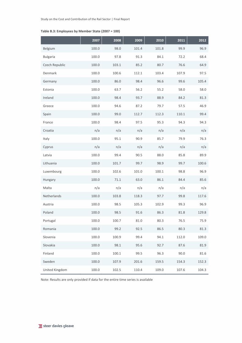
Study on the Cost and Contribution of the Rail Sector | Final Report
Table B.3: Employees by Member State (2007 = 100)
2007 2008 2009 2010 2011 2012
Belgium 100.0 98.0 101.4 101.8 99.9 96.9
Bulgaria 100.0 97.8 91.3 84.1 72.2 68.4
Czech Republic 100.0 103.1 85.2 80.7 76.6 64.9
Denmark 100.0 100.6 112.1 103.4 107.9 97.5
Germany 100.0 86.0 98.4 96.6 99.6 105.4
Estonia 100.0 63.7 56.2 55.2 58.0 58.0
Ireland 100.0 98.4 93.7 88.9 84.2 81.3
Greece 100.0 94.6 87.2 79.7 57.5 46.9
Spain 100.0 99.0 112.7 112.3 110.1 99.4
France 100.0 98.4 97.5 95.3 94.3 94.3
Croatia n/a n/a n/a n/a n/a n/a
Italy 100.0 95.1 90.9 85.7 79.9 76.3
Cyprus n/a n/a n/a n/a n/a n/a
Latvia 100.0 99.4 90.5 88.0 85.8 89.9
Lithuania 100.0 101.7 99.7 98.9 99.7 100.6
Luxembourg 100.0 102.6 101.0 100.1 98.8 96.9
Hungary 100.0 71.1 63.0 86.1 84.4 85.6
Malta n/a n/a n/a n/a n/a n/a
Netherlands 100.0 103.8 118.3 97.7 99.8 117.6
Austria 100.0 98.5 105.3 102.9 99.3 96.9
Poland 100.0 98.5 91.6 86.3 81.8 129.8
Portugal 100.0 100.7 81.0 80.3 76.5 75.9
Romania 100.0 99.2 92.5 86.5 80.3 81.3
Slovenia 100.0 100.9 99.4 94.1 112.0 109.0
Slovakia 100.0 98.1 95.6 92.7 87.6 81.9
Finland 100.0 100.1 99.5 96.3 90.0 81.6
Sweden 100.0 107.9 201.6 159.5 154.3 152.3
United Kingdom 100.0 102.5 110.4 109.0 107.6 104.3
Note: Results are only provided if data for the entire time series is available
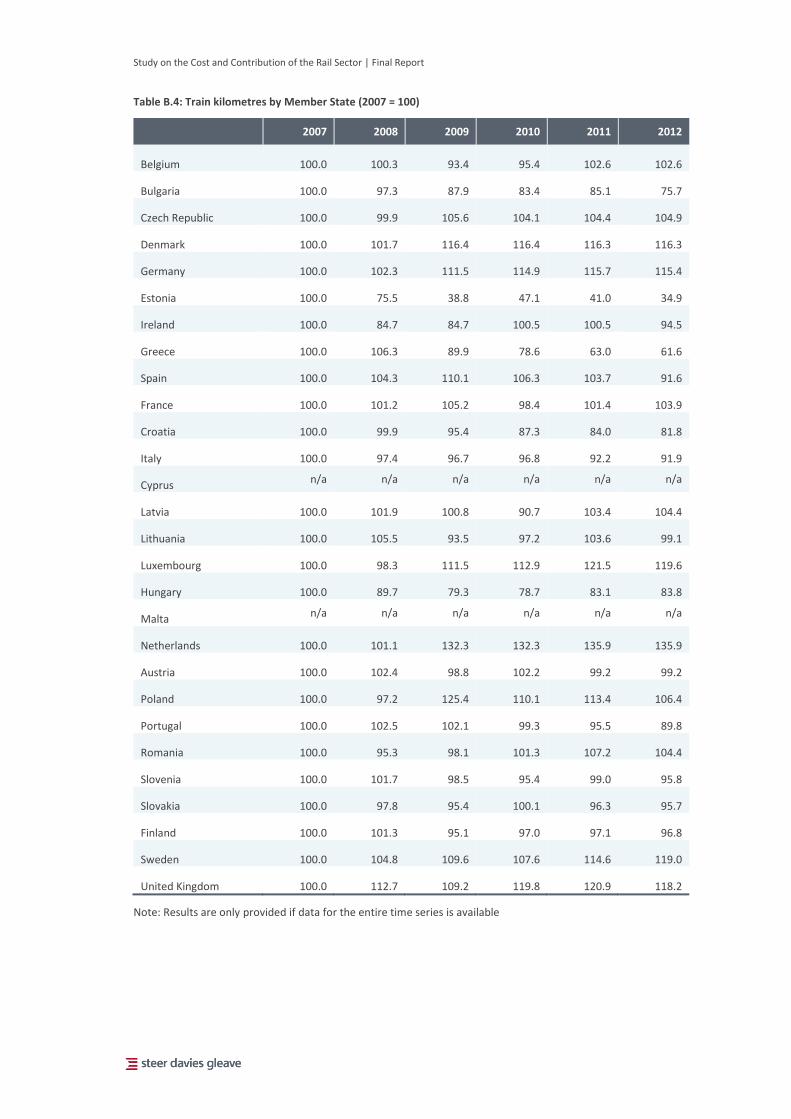
Study on the Cost and Contribution of the Rail Sector | Final Report
Table B.4: Train kilometres by Member State (2007 = 100)
2007 2008 2009 2010 2011 2012
Belgium 100.0 100.3 93.4 95.4 102.6 102.6
Bulgaria 100.0 97.3 87.9 83.4 85.1 75.7
Czech Republic 100.0 99.9 105.6 104.1 104.4 104.9
Denmark 100.0 101.7 116.4 116.4 116.3 116.3
Germany 100.0 102.3 111.5 114.9 115.7 115.4
Estonia 100.0 75.5 38.8 47.1 41.0 34.9
Ireland 100.0 84.7 84.7 100.5 100.5 94.5
Greece 100.0 106.3 89.9 78.6 63.0 61.6
Spain 100.0 104.3 110.1 106.3 103.7 91.6
France 100.0 101.2 105.2 98.4 101.4 103.9
Croatia 100.0 99.9 95.4 87.3 84.0 81.8
Italy 100.0 97.4 96.7 96.8 92.2 91.9
Cyprus n/a n/a n/a n/a n/a n/a
Latvia 100.0 101.9 100.8 90.7 103.4 104.4
Lithuania 100.0 105.5 93.5 97.2 103.6 99.1
Luxembourg 100.0 98.3 111.5 112.9 121.5 119.6
Hungary 100.0 89.7 79.3 78.7 83.1 83.8
Malta n/a n/a n/a n/a n/a n/a
Netherlands 100.0 101.1 132.3 132.3 135.9 135.9
Austria 100.0 102.4 98.8 102.2 99.2 99.2
Poland 100.0 97.2 125.4 110.1 113.4 106.4
Portugal 100.0 102.5 102.1 99.3 95.5 89.8
Romania 100.0 95.3 98.1 101.3 107.2 104.4
Slovenia 100.0 101.7 98.5 95.4 99.0 95.8
Slovakia 100.0 97.8 95.4 100.1 96.3 95.7
Finland 100.0 101.3 95.1 97.0 97.1 96.8
Sweden 100.0 104.8 109.6 107.6 114.6 119.0
United Kingdom 100.0 112.7 109.2 119.8 120.9 118.2
Note: Results are only provided if data for the entire time series is available

Study on the Cost and Contribution of the Rail Sector | Final Report
Table B.5: Rail passenger kilometres by Member State (2007 = 100)
2007 2008 2009 2010 2011 2012
Belgium 100.0 104.7 105.2 106.4 105.1 103.7
Bulgaria 100.0 96.4 88.5 86.7 85.3 77.4
Czech Republic 100.0 98.6 94.3 95.5 97.3 105.3
Denmark 100.0 101.7 99.6 102.8 107.0 109.3
Germany 100.0 104.3 104.0 106.1 107.6 111.8
Estonia 100.0 100.1 91.1 90.5 88.8 85.9
Ireland 100.0 98.5 83.9 83.6 81.6 78.6
Greece 100.0 85.7 73.2 69.2 49.6 43.0
Spain 100.0 109.7 105.9 102.4 104.3 102.8
France 100.0 106.2 105.3 105.3 109.1 109.2
Croatia 100.0 112.4 113.9 108.1 92.2 68.5
Italy 100.0 99.5 96.7 94.8 94.1 89.6
Cyprus n/a n/a n/a n/a n/a n/a
Latvia 100.0 96.7 76.9 76.2 75.4 74.2
Lithuania 100.0 97.3 87.3 91.2 95.1 98.5
Luxembourg 100.0 109.2 105.4 109.8 110.4 118.4
Hungary 100.0 94.8 92.2 87.9 89.2 89.2
Malta n/a n/a n/a n/a n/a n/a
Netherlands 100.0 98.5 99.1 99.1 108.1 110.0
Austria 100.0 113.1 111.2 112.1 113.5 118.2
Poland 100.0 101.7 93.8 90.2 91.5 89.8
Portugal 100.0 105.7 104.1 103.1 103.9 95.4
Romania 100.0 93.1 82.0 72.7 67.7 60.9
Slovenia 100.0 102.7 103.4 100.1 95.2 91.3
Slovakia 100.0 106.1 104.6 106.7 112.3 113.6
Finland 100.0 107.3 102.6 104.8 102.8 106.8
Sweden 100.0 108.6 110.3 108.7 110.9 114.9
United Kingdom 100.0 105.6 105.2 111.3 116.8 121.5
Note: Results are only provided if data for the entire time series is available
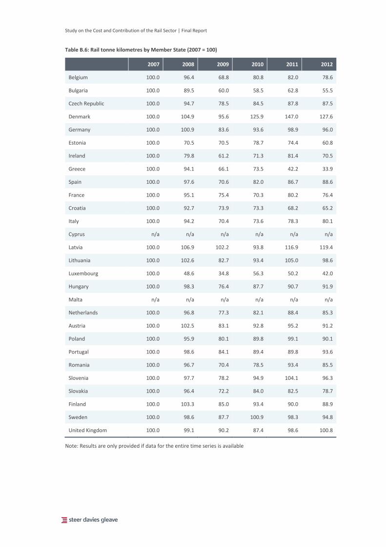
Study on the Cost and Contribution of the Rail Sector | Final Report
Table B.6: Rail tonne kilometres by Member State (2007 = 100)
2007 2008 2009 2010 2011 2012
Belgium 100.0 96.4 68.8 80.8 82.0 78.6
Bulgaria 100.0 89.5 60.0 58.5 62.8 55.5
Czech Republic 100.0 94.7 78.5 84.5 87.8 87.5
Denmark 100.0 104.9 95.6 125.9 147.0 127.6
Germany 100.0 100.9 83.6 93.6 98.9 96.0
Estonia 100.0 70.5 70.5 78.7 74.4 60.8
Ireland 100.0 79.8 61.2 71.3 81.4 70.5
Greece 100.0 94.1 66.1 73.5 42.2 33.9
Spain 100.0 97.6 70.6 82.0 86.7 88.6
France 100.0 95.1 75.4 70.3 80.2 76.4
Croatia 100.0 92.7 73.9 73.3 68.2 65.2
Italy 100.0 94.2 70.4 73.6 78.3 80.1
Cyprus n/a n/a n/a n/a n/a n/a
Latvia 100.0 106.9 102.2 93.8 116.9 119.4
Lithuania 100.0 102.6 82.7 93.4 105.0 98.6
Luxembourg 100.0 48.6 34.8 56.3 50.2 42.0
Hungary 100.0 98.3 76.4 87.7 90.7 91.9
Malta n/a n/a n/a n/a n/a n/a
Netherlands 100.0 96.8 77.3 82.1 88.4 85.3
Austria 100.0 102.5 83.1 92.8 95.2 91.2
Poland 100.0 95.9 80.1 89.8 99.1 90.1
Portugal 100.0 98.6 84.1 89.4 89.8 93.6
Romania 100.0 96.7 70.4 78.5 93.4 85.5
Slovenia 100.0 97.7 78.2 94.9 104.1 96.3
Slovakia 100.0 96.4 72.2 84.0 82.5 78.7
Finland 100.0 103.3 85.0 93.4 90.0 88.9
Sweden 100.0 98.6 87.7 100.9 98.3 94.8
United Kingdom 100.0 99.1 90.2 87.4 98.6 100.8
Note: Results are only provided if data for the entire time series is available

Study on the Cost and Contribution of the Rail Sector | Final Report
Table B.7: Passenger revenue by Member State (2007 = 100)
2007 2008 2009 2010 2011 2012
Belgium 100.0 107.3 109.5 113.0 114.5 114.9
Bulgaria 100.0 109.2 100.8 96.1 98.4 96.1
Czech Republic 100.0 107.9 106.4 113.2 121.8 124.8
Denmark 100.0 103.5 96.4 98.8 127.0 108.9
Germany 100.0 107.2 106.9 107.5 109.5 128.0
Estonia 100.0 116.2 118.0 114.1 117.3 108.3
Ireland 100.0 102.0 93.8 86.7 83.0 89.1
Greece 100.0 99.0 102.6 109.8 91.2 103.3
Spain 100.0 125.7 136.4 139.7 148.6 145.8
France* 100.0 124.5 150.6 166.5 189.9 192.9
Croatia n/a n/a n/a n/a n/a n/a
Italy 100.0 104.6 107.3 109.9 114.0 113.0
Cyprus n/a n/a n/a n/a n/a n/a
Latvia 100.0 26.1 27.0 26.3 25.1 5.9
Lithuania 100.0 109.2 101.9 117.0 130.0 137.7
Luxembourg 100.0 104.6 107.7 117.2 119.7 123.6
Hungary 100.0 12.4 169.1 180.1 190.4 187.0
Malta n/a n/a n/a n/a n/a n/a
Netherlands 100.0 102.9 107.3 110.6 117.8 120.2
Austria 100.0 113.6 111.7 89.8 90.6 94.9
Poland* 100.0 154.6 178.6 209.6 175.6 409.9
Portugal 100.0 107.2 107.2 109.2 111.5 112.3
Romania 100.0 97.9 74.9 71.0 78.1 73.9
Slovenia 100.0 105.3 104.6 104.3 111.2 119.3
Slovakia 100.0 115.4 111.9 113.9 125.3 139.5
Finland 100.0 110.9 110.6 113.9 113.5 120.7
Sweden 100.0 103.5 87.6 95.0 87.3 90.2
United Kingdom 100.0 102.3 96.1 105.2 111.2 130.0
Note: Results are only provided if data for the entire time series is available (* Passenger revenue in Poland is considerably higher in 2012 when compared to previous years and is a result of improved coverage of our dataset in 2012 compared to previous time periods)

Study on the Cost and Contribution of the Rail Sector | Final Report
Table B.8: Operating costs (operator and infrastructure manager) by Member State (2007 = 100)
2007 2008 2009 2010 2011 2012
Belgium 100.0 105.3 110.5 123.5 112.9 111.9
Bulgaria 100.0 111.1 95.6 86.1 82.8 88.3
Czech Republic 100.0 128.6 120.6 120.1 115.9 125.2
Denmark 100.0 104.2 111.5 122.7 130.7 123.0
Germany 100.0 101.6 99.9 102.0 101.9 117.8
Estonia n/a n/a n/a n/a n/a n/a
Ireland 100.0 105.0 96.0 90.6 80.0 78.6
Greece 100.0 101.2 104.8 92.8 140.8 69.2
Spain 100.0 109.9 118.8 119.1 138.7 128.0
France 100.0 102.0 109.7 126.9 132.5 129.6
Croatia n/a n/a n/a n/a n/a n/a
Italy 100.0 101.2 93.9 83.9 84.3 83.8
Cyprus n/a n/a n/a n/a n/a n/a
Latvia n/a n/a n/a n/a n/a n/a
Lithuania 100.0 118.3 99.3 108.5 120.6 130.7
Luxembourg 100.0 103.0 101.0 175.1 191.9 196.9
Hungary 100.0 130.7 71.7 72.6 74.7 78.2
Malta n/a n/a n/a n/a n/a n/a
Netherlands 100.0 105.8 93.6 103.0 102.8 113.6
Austria 100.0 118.0 123.7 129.2 129.2 127.9
Poland 100.0 128.6 95.9 108.7 126.8 98.7
Portugal 100.0 104.8 101.8 102.1 116.4 105.5
Romania 100.0 100.1 80.2 111.9 130.2 138.3
Slovenia 100.0 110.0 105.4 113.8 150.5 137.8
Slovakia 100.0 121.9 125.2 120.1 116.8 115.4
Finland 100.0 102.6 105.3 100.5 103.3 97.6
Sweden 100.0 105.9 105.8 109.2 154.0 166.9
United Kingdom 100.0 101.7 90.9 94.3 96.1 114.5
Note: Results are only provided if data for the entire time series is available
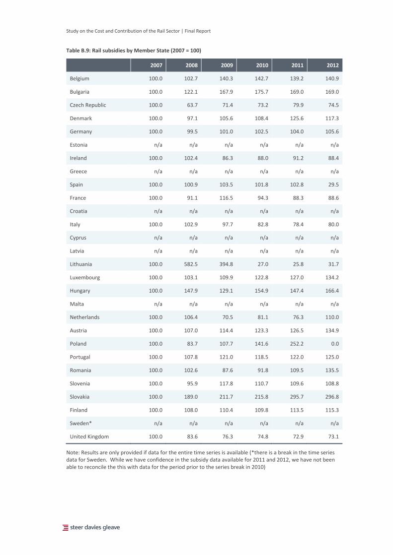
Study on the Cost and Contribution of the Rail Sector | Final Report
Table B.9: Rail subsidies by Member State (2007 = 100)
2007 2008 2009 2010 2011 2012
Belgium 100.0 102.7 140.3 142.7 139.2 140.9
Bulgaria 100.0 122.1 167.9 175.7 169.0 169.0
Czech Republic 100.0 63.7 71.4 73.2 79.9 74.5
Denmark 100.0 97.1 105.6 108.4 125.6 117.3
Germany 100.0 99.5 101.0 102.5 104.0 105.6
Estonia n/a n/a n/a n/a n/a n/a
Ireland 100.0 102.4 86.3 88.0 91.2 88.4
Greece n/a n/a n/a n/a n/a n/a
Spain 100.0 100.9 103.5 101.8 102.8 29.5
France 100.0 91.1 116.5 94.3 88.3 88.6
Croatia n/a n/a n/a n/a n/a n/a
Italy 100.0 102.9 97.7 82.8 78.4 80.0
Cyprus n/a n/a n/a n/a n/a n/a
Latvia n/a n/a n/a n/a n/a n/a
Lithuania 100.0 582.5 394.8 27.0 25.8 31.7
Luxembourg 100.0 103.1 109.9 122.8 127.0 134.2
Hungary 100.0 147.9 129.1 154.9 147.4 166.4
Malta n/a n/a n/a n/a n/a n/a
Netherlands 100.0 106.4 70.5 81.1 76.3 110.0
Austria 100.0 107.0 114.4 123.3 126.5 134.9
Poland 100.0 83.7 107.7 141.6 252.2 0.0
Portugal 100.0 107.8 121.0 118.5 122.0 125.0
Romania 100.0 102.6 87.6 91.8 109.5 135.5
Slovenia 100.0 95.9 117.8 110.7 109.6 108.8
Slovakia 100.0 189.0 211.7 215.8 295.7 296.8
Finland 100.0 108.0 110.4 109.8 113.5 115.3
Sweden* n/a n/a n/a n/a n/a n/a
United Kingdom 100.0 83.6 76.3 74.8 72.9 73.1
Note: Results are only provided if data for the entire time series is available (*there is a break in the time series data for Sweden. While we have confidence in the subsidy data available for 2011 and 2012, we have not been able to reconcile the this with data for the period prior to the series break in 2010)

Study on the Cost and Contribution of the Rail Sector | Final Report
Table B.10: Track utilisation by Member State (total train kilometres/track kilometres)
2007 2008 2009 2010 2011 2012
Belgium
29,243
28,159
25,748
26,271
28,273
28,273
Bulgaria
8,862
8,623
7,778
7,478
7,673
6,830
Czech Republic
16,049
16,213
17,148
16,920
16,959
17,045
Denmark
21,440
21,794
24,949
24,949
25,105
25,114
Germany
26,537
27,171
29,737
30,662
30,986
30,959
Estonia
11,183
7,499
3,849
5,461
4,724
4,021
Ireland
8,771
7,428
7,428
8,819
8,819
8,286
Greece
7,803
8,293
7,014
6,130
4,908
4,800
Spain
12,915
13,471
14,425
13,484
13,071
11,556
France
16,462
16,676
17,331
16,228
16,422
16,740
Croatia
10,842
10,836
10,341
9,469
9,102
8,870
Italy
20,653
19,889
19,574
19,579
18,620
18,549
Latvia
7,853
8,009
9,516
8,503
9,861
9,983
Lithuania
8,489
8,961
7,935
8,243
8,786
8,409
Luxembourg
26,287
25,851
29,313
29,676
31,931
31,440
Hungary
15,719
14,182
12,545
12,443
13,118
13,286
Netherlands
37,952
38,267
48,125
48,125
49,452
49,452
Austria
24,140
25,387
25,897
28,483
27,744
28,464
Poland
10,086
9,701
12,428
10,950
11,263
10,620
Portugal
13,722
14,046
13,998
13,603
13,318
13,769
Romania
8,569
8,164
8,403
8,678
9,185
8,946
Slovenia
16,093
16,366
15,856
15,345
16,180
15,667
Slovakia
12,991
12,720
12,409
13,035
12,525
12,557
Finland
8,913
8,998
8,451
8,616
8,592
8,562
Sweden
11,165
11,635
12,050
11,808
12,524
13,086
United Kingdom
28,851
32,510
31,627
34,641
34,457
33,675
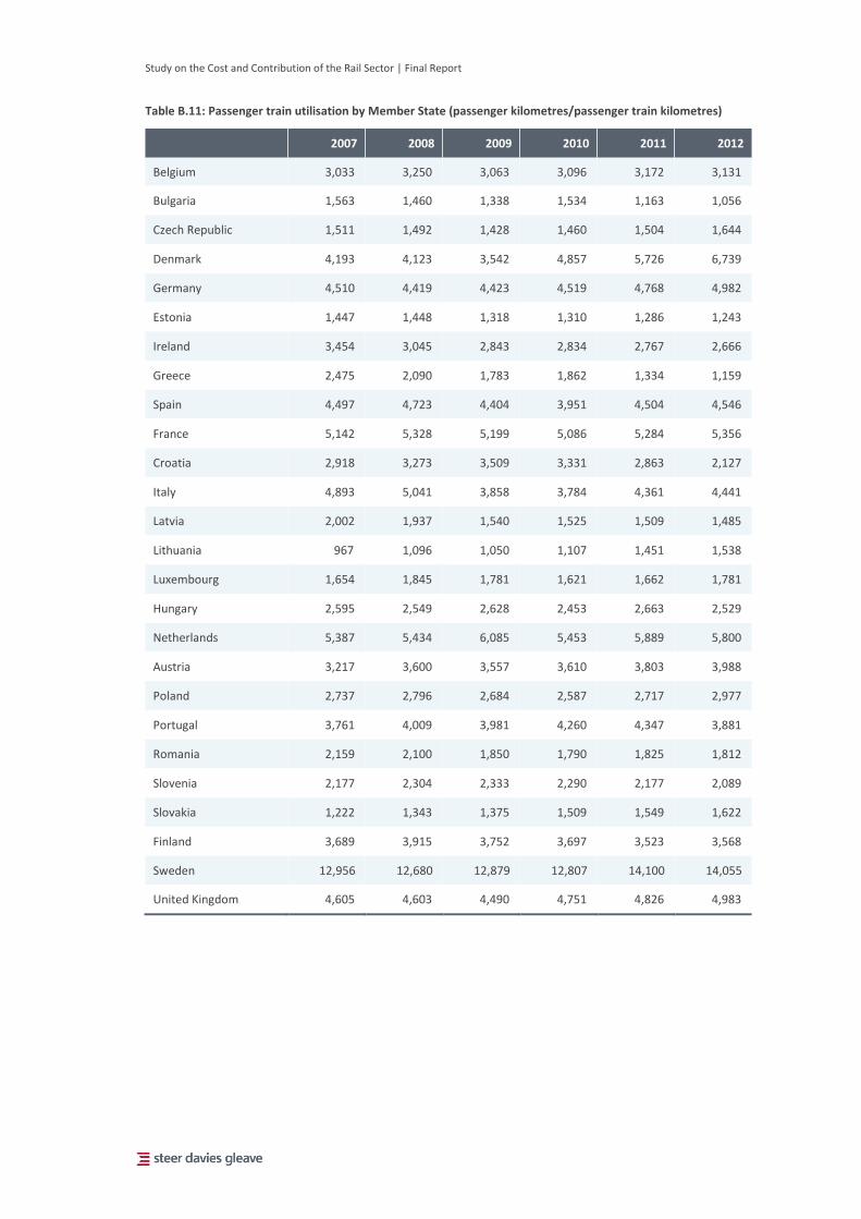
Study on the Cost and Contribution of the Rail Sector | Final Report
Table B.11: Passenger train utilisation by Member State (passenger kilometres/passenger train kilometres)
2007 2008 2009 2010 2011 2012
Belgium 3,033 3,250 3,063 3,096 3,172 3,131
Bulgaria 1,563 1,460 1,338 1,534 1,163 1,056
Czech Republic 1,511 1,492 1,428 1,460 1,504 1,644
Denmark 4,193 4,123 3,542 4,857 5,726 6,739
Germany 4,510 4,419 4,423 4,519 4,768 4,982
Estonia 1,447 1,448 1,318 1,310 1,286 1,243
Ireland 3,454 3,045 2,843 2,834 2,767 2,666
Greece 2,475 2,090 1,783 1,862 1,334 1,159
Spain 4,497 4,723 4,404 3,951 4,504 4,546
France 5,142 5,328 5,199 5,086 5,284 5,356
Croatia 2,918 3,273 3,509 3,331 2,863 2,127
Italy 4,893 5,041 3,858 3,784 4,361 4,441
Latvia 2,002 1,937 1,540 1,525 1,509 1,485
Lithuania 967 1,096 1,050 1,107 1,451 1,538
Luxembourg 1,654 1,845 1,781 1,621 1,662 1,781
Hungary 2,595 2,549 2,628 2,453 2,663 2,529
Netherlands 5,387 5,434 6,085 5,453 5,889 5,800
Austria 3,217 3,600 3,557 3,610 3,803 3,988
Poland 2,737 2,796 2,684 2,587 2,717 2,977
Portugal 3,761 4,009 3,981 4,260 4,347 3,881
Romania 2,159 2,100 1,850 1,790 1,825 1,812
Slovenia 2,177 2,304 2,333 2,290 2,177 2,089
Slovakia 1,222 1,343 1,375 1,509 1,549 1,622
Finland 3,689 3,915 3,752 3,697 3,523 3,568
Sweden 12,956 12,680 12,879 12,807 14,100 14,055
United Kingdom 4,605 4,603 4,490 4,751 4,826 4,983

Study on the Cost and Contribution of the Rail Sector | Final Report
Table B.12: Freight train utilisation by Member State (freight tonne kilometres/freight train kilometres)
2007 2008 2009 2010 2011 2012
Belgium 589 563 497 644 654 627
Bulgaria 422 366 266 261 200 175
Czech Republic 342 329 361 502 524 527
Denmark 809 848 773 1,018 1,191 1,035
Germany 776 659 533 625 646 642
Estonia 429 303 325 378 355 289
Ireland 145 116 113 183 209 181
Greece 234 165 116 194 111 90
Spain 724 733 638 642 710 704
France 566 528 455 400 475 469
Croatia 527 499 398 392 402 385
Italy 610 584 587 614 694 914
Latvia 3,484 3,745 3,099 2,845 3,495 3,460
Lithuania 1,515 1,529 1,243 1,454 1,638 1,555
Luxembourg 163 73 51 83 74 62
Hungary 857 839 656 753 779 789
Netherlands 2,844 2,567 1,922 1,920 1,952 1,784
Austria 1,157 718 654 693 1,168 1,077
Poland 733 699 597 715 826 773
Portugal 876 838 714 724 732 764
Romania 294 325 237 170 212 185
Slovenia 906 898 721 1,065 1,194 1,112
Slovakia 533 530 404 478 460 443
Finland 967 986 843 932 907 945
Sweden 1,463 1,457 1,378 1,547 1,531 1,498
United Kingdom 669 676 641 663 769 808
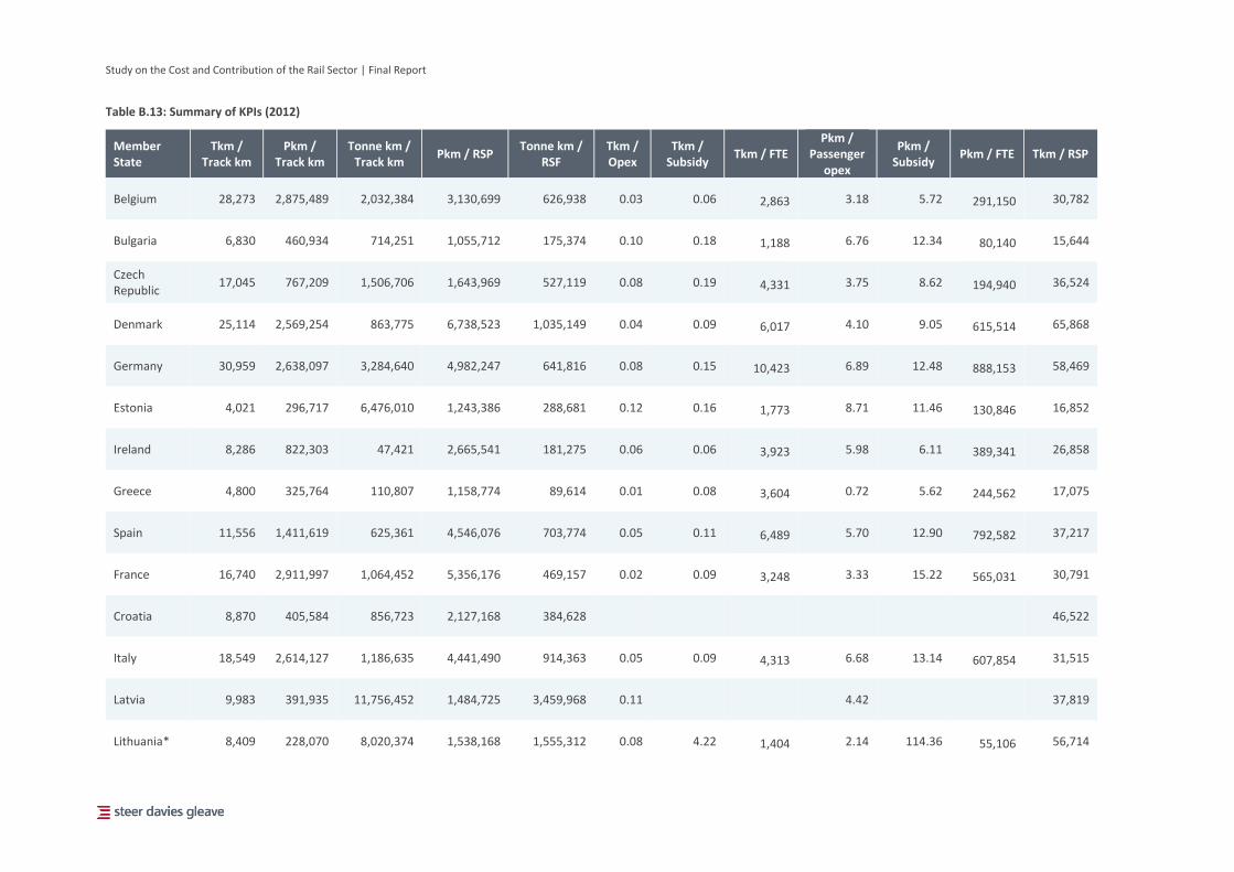
Study on the Cost and Contribution of the Rail Sector | Final Report
Table B.13: Summary of KPIs (2012)
Member State
Tkm / Track km
Pkm / Track km
Tonne km / Track km
Pkm / RSP Tonne km /
RSF Tkm / Opex
Tkm / Subsidy
Tkm / FTE Pkm /
Passenger opex
Pkm / Subsidy
Pkm / FTE Tkm / RSP
Belgium 28,273 2,875,489 2,032,384 3,130,699 626,938 0.03 0.06 2,863 3.18 5.72 291,150 30,782
Bulgaria 6,830 460,934 714,251 1,055,712 175,374 0.10 0.18 1,188 6.76 12.34 80,140 15,644
Czech Republic
17,045 767,209 1,506,706 1,643,969 527,119 0.08 0.19 4,331 3.75 8.62 194,940 36,524
Denmark 25,114 2,569,254 863,775 6,738,523 1,035,149 0.04 0.09 6,017 4.10 9.05 615,514 65,868
Germany 30,959 2,638,097 3,284,640 4,982,247 641,816 0.08 0.15 10,423 6.89 12.48 888,153 58,469
Estonia 4,021 296,717 6,476,010 1,243,386 288,681 0.12 0.16 1,773 8.71 11.46 130,846 16,852
Ireland 8,286 822,303 47,421 2,665,541 181,275 0.06 0.06 3,923 5.98 6.11 389,341 26,858
Greece 4,800 325,764 110,807 1,158,774 89,614 0.01 0.08 3,604 0.72 5.62 244,562 17,075
Spain 11,556 1,411,619 625,361 4,546,076 703,774 0.05 0.11 6,489 5.70 12.90 792,582 37,217
France 16,740 2,911,997 1,064,452 5,356,176 469,157 0.02 0.09 3,248 3.33 15.22 565,031 30,791
Croatia 8,870 405,584 856,723 2,127,168 384,628
46,522
Italy 18,549 2,614,127 1,186,635 4,441,490 914,363 0.05 0.09 4,313 6.68 13.14 607,854 31,515
Latvia 9,983 391,935 11,756,452 1,484,725 3,459,968 0.11
4.42
37,819
Lithuania* 8,409 228,070 8,020,374 1,538,168 1,555,312 0.08 4.22 1,404 2.14 114.36 55,106 56,714

Study on the Cost and Contribution of the Rail Sector | Final Report
Luxembourg 31,440 1,360,000 876,364 1,780,952 61,874 0.02 0.05 1,402 0.99 2.14 38,015 41,171
Hungary 13,286 990,990 1,171,766 2,529,497 788,889 0.08 0.12 2,667 5.75 8.85 115,361 33,913
Netherlands 49,452 5,674,743 2,043,478 5,799,864 1,784,262 0.03 0.05 2,683 3.22 5.57 200,144 50,543
Austria 28,464 2,313,649 3,984,266 3,988,376 1,077,055 0.04 0.06
2.98 5.09
49,067
Poland 10,620 908,702 2,492,889 2,977,451 772,938 0.10 0.20 4,407 8.30 16.71 505,701 34,796
Portugal 13,769 1,496,655 952,774 3,880,612 763,722 0.04 0.47 3,353 4.21 50.63 272,561 35,700
Romania 8,946 422,195 1,250,070 1,812,027 185,468 0.06 0.24 1,300 2.95 11.12 111,270 38,394
Slovenia 15,667 613,482 2,870,141 2,089,296 1,112,179 0.10 0.43 5,564 3.99 16.77 604,778 53,355
Slovakia 12,557 684,386 2,112,719 1,622,032 442,753 0.05 0.10 1,877 2.88 5.18 88,599 29,761
Finland 8,562 678,836 1,560,397 3,567,639 944,790 0.05 0.36 2,190 4.21 28.16 85,765 44,996
Sweden^ 13,086 1,058,908 1,979,436 14,054,827 1,498,442 0.08 0.23 1,630 6.14 18.93 88,819 173,695
United Kingdom
33,675 3,712,111 1,305,730 4,983,162 807,524 0.04 0.11 6,175 4.32 12.58 489,625 45,205
Source: SDG analysis (TKm = train kilometres; Pkm – passenger kilometres; RSP = passenger rolling stock; RSF = freight rolling stock; Opex = total operating costs; Passenger opex = passenger operating costs; FTE = full time equivalent employees) * Subsidy data for Lithuania appear volatile over time and therefore Tkm/subsidy and Tkm/subsidy figures may be over-stated ^ Passenger rolling stock quantities for Sweden appear very small compared to the size of the rail network (this is consistent through time)
Study on the Cost and Contribution of the Rail Sector | Final Report
C Clustering methods C.1 In determining our approach to clustering, we considered three distinct yet complementary
methodologies that appeared promising but which were ultimately discarded. These were:
Regression modelling;
Hierarchical partitioning; and
Expert review.
Regression modelling
C.2 Our first approach to clustering used regression modelling in which a normalised measure of
performance (e.g. passenger-kilometre per capita) was used as the dependent variable of a
regression model. The exogenous factors identified above were then treated as independent
variables that have an influence on performance. In performing this analysis we:
Obtained factor-specific coefficients by way of a OLS/logit regression;
Used these coefficients as inputs into a modelled function for each Member State
Used outturn data for the exogenous variables to estimate the expected value of the
dependent variable48;
Ranked Member States based on those scores; and
Allocated Member States to clusters according to the frequency with which they were
ranked in a given quartile across models.
C.3 Regression modelling is more data-driven and potentially more objective than other methods,
but the results are based on the assumption that the main exogenous determinants of key
performance have been included in the analysis.
Hierarchical partitioning
C.4 Our second approach involved hierarchical clustering by way of partitioning. Exogenous
factors were ranked in terms of their statistical significance using outputs from the regression
analysis49. We then constructed a tree diagram based on thresholds that are set at the mean
value for each of the exogenous factors. For instance, Member States were first divided into
two groups depending on whether their GDP per capita (identified as the most important
48 Either as an absolute number (from the OLS regression) or as a probability score (from the logit
regression)
49 GDP per capita was the most important variable, followed by population density, track density, and
number of ports linked by rail. High-speed rail network length was not included in the partitioning in
order to reduce the number of branches created.

Study on the Cost and Contribution of the Rail Sector | Final Report
influence on rail performance) was above or below the average GDP per capita for the EU26.
Next, the group of wealthier Member States was split according to whether the population
density (the second most important influence on performance) was above or below the
average.
C.5 Hierarchical partitioning is more flexible and gives greater weight to the exogenous factors
that are deemed to be most important, such as GDP per capita. However, it requires
assumptions about the thresholds underpinning each partition and led to a greater level of
disaggregation than was required for the analysis.
Expert review
C.6 The third approach relied heavily on expert judgement. While broadly comparable to the
method of hierarchical clustering, this approach built clusters from the bottom-up. We created
13 pairs of Member States based on a review of exogenous factors, and consideration of
similarities and differences in rail markets from previous studies. Having identified the pairs of
‘most similar’ Member States, we then aggregated those pairs into larger groups based on the
similarities between pairs. This was based on an inspection of the available data on
exogenous factors, as well as knowledge of other systems of classification adopted by EU
institutions. For example, the Cohesion Funding Framework 2014-2020 indicates which
countries are eligible for EU funds based on an index of socio-economic indicators and allows
groupings according to classifications such as ‘more developed’ or ‘transition’ Member States.
The Global Competitiveness Index prepared by the World Economic Forum similarly provided
useful information on the quality of perceived transport infrastructure. While the approach
allows greater flexibility, it is clearly subjective and therefore particularly open to challenge.

Study on the Cost and Contribution of the Rail Sector | Final Report
D Clustering outputs D.1 Table C.1 reports the results of the nine clustering model specifications described in Table 4.3.
The results are presented against a ‘five-cluster’ specification. While models 4 and 8 were
identified as our preferred models from a passenger and freight perspective, it should be
noted that further professional experience and judgement was applied in order to determine
the final clusters used in subsequent phases of the analysis.
Table D.1: Detailed clustering outputs
Passenger Freight
Model 1 2 3 4 5 6 7 8 9
BE 1 1 1 1 1 1 1 1 1
BG 4 2 2 5 2 2 2 4 2
CZ 4 2 2 5 2 2 2 4 2
DK 2 1 1 1 1 1 1 2 1
DE 1 3 3 3 3 3 3 1 3
EE 4 1 1 5 1 1 1 4 1
IE 2 2 2 1 2 2 2 2 2
EL 5 2 2 5 2 2 2 5 2
ES 5 4 4 4 4 4 4 5 4
FR 1 5 5 3 5 5 5 1 5
HR 4 1 1 5 1 1 1 4 1
IT 5 3 3 4 3 3 3 5 3
LV 4 1 1 5 1 1 1 4 1
LT 4 1 1 5 1 1 1 4 1
LU 3 1 1 2 1 1 1 3 1
HU 4 2 2 5 2 2 2 4 2
NL 1 1 1 1 1 1 1 1 1
AT 1 2 2 1 2 2 2 1 2
PL 4 3 3 5 3 3 3 4 3
PT 5 2 2 5 2 2 2 5 2
RO 4 3 3 5 3 3 3 4 3
SI 5 1 1 5 1 1 1 5 1
SK 4 1 1 5 1 1 1 4 1
FI 1 3 3 1 3 3 3 1 3
SE 2 4 4 4 4 4 4 2 4
UK 1 3 3 4 3 3 3 1 3
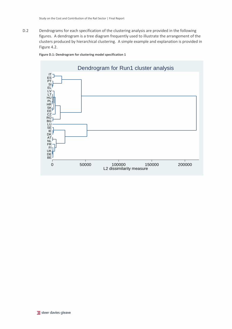
Study on the Cost and Contribution of the Rail Sector | Final Report
D.2 Dendrograms for each specification of the clustering analysis are provided in the following
figures. A dendrogram is a tree diagram frequently used to illustrate the arrangement of the
clusters produced by hierarchical clustering. A simple example and explanation is provided in
Figure 4.2.
Figure D.1: Dendrogram for clustering model specification 1
BEDEUKFI
FRNLATDKIE
SELUBGROCZEESKHRPLHULTLVELSI
PTESIT
0 50000 100000 150000 200000L2 dissimilarity measure
Dendrogram for Run1 cluster analysis

Study on the Cost and Contribution of the Rail Sector | Final Report
Figure D.2: Dendrogram for clustering model specification 2
Figure D.3: Dendrogram for clustering model specification 3
BEDKNLSI
LUEESKHRLVLTBGELCZHUPTIE
ATDEFIIT
PLROUKESSEFR
0 500000 1000000 1500000 2000000 2500000L2 dissimilarity measure
Dendrogram for Run_2 cluster analysis
BEDKNLSI
LUEESKHRLVLTBGELCZHUPTIE
ATDEFIIT
PLROUKESSEFR
0 500000 1000000 1500000 2000000 2500000L2 dissimilarity measure
Dendrogram for Run_3 cluster analysis

Study on the Cost and Contribution of the Rail Sector | Final Report
Figure D.4: Dendrogram for clustering model specification 4
Figure D.5: Dendrogram for clustering model specification 5
BENLATFI
DKIE
LUDEFRESIT
SEUKBGROCZHUPLEEHRLTLVSKELPTSI
0 50000 100000 150000 200000L2 dissimilarity measure
Dendrogram for Run_4 cluster analysis
BEDKNLSI
LUEESKHRLVLTBGELCZHUPTIE
ATDEFIIT
PLROUKESSEFR
0 500000 1000000 1500000 2000000 2500000L2 dissimilarity measure
Dendrogram for Run_5 cluster analysis

Study on the Cost and Contribution of the Rail Sector | Final Report
Figure D.6: Dendrogram for clustering model specification 6
Figure D.7: Dendrogram for clustering model specification 7
BEDKNLSI
LUEESKHRLVLTBGELCZHUPTIE
ATDEFIIT
PLROUKESSEFR
0 500000 1000000 1500000 2000000 2500000L2 dissimilarity measure
Dendrogram for Run_6 cluster analysis
BEDKNLSI
LUEESKHRLVLTBGELCZHUPTIE
ATDEFIIT
PLROUKESSEFR
0 500000 1000000 1500000 2000000 2500000L2 dissimilarity measure
Dendrogram for Run_7 cluster analysis
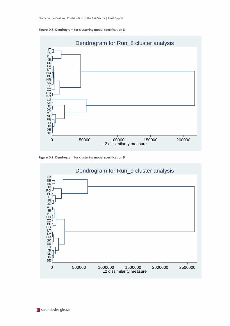
Study on the Cost and Contribution of the Rail Sector | Final Report
Figure D.8: Dendrogram for clustering model specification 8
Figure D.9: Dendrogram for clustering model specification 9
BEDEUKFI
FRNLATDKIE
SELUBGROCZEESKHRPLHULTLVELSI
PTESIT
0 50000 100000 150000 200000L2 dissimilarity measure
Dendrogram for Run_8 cluster analysis
BEDKNLSI
LUEESKHRLVLTBGELCZHUPTIE
ATDEFIIT
PLROUKESSEFR
0 500000 1000000 1500000 2000000 2500000L2 dissimilarity measure
Dendrogram for Run_9 cluster analysis

Study on the Cost and Contribution of the Rail Sector | Final Report
E Data envelopment analysis models E.1 Given the flexibility of DEA to incorporate measures of inputs and outputs across multiple
dimensions, we followed a systematic but iterative approach to analyse the efficiency of
national railway systems. The following pages present results for a sample of the DEA models
tested and as described in Table 5.1, under both constant and variable returns to scale
assumptions.
Table E.1: Data envelopment analysis outputs – variable returns to scale (mean)
Total capital productivity
(static)
Total capital productivity
(dynamic)
Passenger only
Freight only Track
utilisation Train
utilisation
DEA model 1 2 3 4 5 6
Cluster A 0.85 0.85 0.74 0.61 0.62 0.79
Cluster B 0.95 0.94 0.90 0.42 0.73 0.95
Cluster C 0.44 0.46 0.30 0.33 0.28 0.40
Cluster D 0.79 0.81 0.57 0.66 0.50 0.78
EU26 0.78 0.78 0.64 0.53 0.54 0.75
Table E.2: Data envelopment analysis outputs – variable returns to scale (standard deviation)
Total capital productivity
(static)
Total capital productivity
(dynamic)
Passenger only
Freight only Track
utilisation Train
utilisation
DEA model 1 2 3 4 5 6
Cluster A 0.20 0.20 0.25 0.30 0.32 0.26
Cluser B 0.10 0.10 0.13 0.30 0.32 0.10
Cluster C 0.30 0.31 0.09 0.32 0.18 0.32
Cluster D 0.24 0.24 0.23 0.26 0.31 0.26
EU26 0.27 0.27 0.28 0.30 0.32 0.30

Study on the Cost and Contribution of the Rail Sector | Final Report
Table E.3: Data envelopment analysis outputs – variable returns to scale (direct results)
Total capital productivity
(static)
Total capital productivity
(dynamic)
Passenger only
Freight only Track
utilisation Train
utilisation
Cluster DEA model 1 2 3 4 5 6
A
Belgium 0.60 0.62 0.55 0.33 0.60 0.44
Denmark 1.00 1.00 1.00 0.66 0.50 1.00
Ireland 1.00 1.00 0.54 1.00 0.25 1.00
Luxembourg 1.00 1.00 1.00 1.00 1.00 1.00
Netherlands 1.00 1.00 1.00 0.63 1.00 1.00
Austria 0.79 0.78 0.64 0.34 0.77 0.59
Finland 0.54 0.55 0.46 0.31 0.24 0.54
B
Germany 1.00 1.00 0.93 1.00 1.00 1.00
Spain 0.76 0.77 0.68 0.22 0.31 0.76
France 1.00 1.00 1.00 0.38 1.00 1.00
Italy 0.92 0.86 0.81 0.27 0.70 0.92
Sweden 1.00 1.00 1.00 0.44 0.38 1.00
United Kingdom 1.00 1.00 1.00 0.23 1.00 1.00
C
Bulgaria 0.24 0.27 0.22 0.21 0.17 0.23
Czech Republic 0.30 0.28 0.26 0.18 0.24 0.25
Hungary 0.41 0.43 0.37 0.25 0.25 0.39
Poland 0.96 1.00 0.42 0.90 0.59 0.96
Romania 0.30 0.31 0.25 0.12 0.17 0.18
D
Estonia 1.00 1.00 1.00 0.80 0.80 1.00
Greece 0.61 0.61 0.32 0.54 0.13 0.61
Croatia 0.62 0.67 0.47 0.43 0.19 0.62
Latvia 1.00 1.00 0.45 1.00 1.00 1.00
Lithuania 1.00 1.00 0.76 0.73 0.73 1.00
Portugal 0.74 0.83 0.63 0.60 0.36 0.72
Slovenia 1.00 1.00 0.63 0.95 0.46 1.00
Slovakia 0.38 0.36 0.31 0.26 0.30 0.30

Study on the Cost and Contribution of the Rail Sector | Final Report
Table E.4: Data envelopment analysis outputs – variable returns to scale (re-based outputs results)
Total capital productivity
(static)
Total capital productivity
(dynamic)
Passenger only
Freight only Track
utilisation Train
utilisation
Cluster DEA model 1 2 3 4 5 6
A
Belgium 0.60 0.62 0.55 0.33 0.60 0.44
Denmark 1.00 1.00 1.00 0.66 0.50 1.00
Ireland 1.00 1.00 0.54 1.00 0.25 1.00
Luxembourg 1.00 1.00 1.00 1.00 1.00 1.00
Netherlands 1.00 1.00 1.00 0.63 1.00 1.00
Austria 0.79 0.78 0.64 0.34 0.77 0.59
Finland 0.54 0.55 0.46 0.31 0.24 0.54
B
Germany 1.00 1.00 0.93 1.00 1.00 1.00
Spain 0.76 0.77 0.68 0.22 0.31 0.76
France 1.00 1.00 1.00 0.38 1.00 1.00
Italy 0.92 0.86 0.81 0.27 0.70 0.92
Sweden 1.00 1.00 1.00 0.44 0.38 1.00
United Kingdom 1.00 1.00 1.00 0.23 1.00 1.00
C
Bulgaria 0.25 0.27 0.52 0.23 0.28 0.24
Czech Republic 0.32 0.28 0.61 0.19 0.40 0.25
Hungary 0.42 0.43 0.88 0.28 0.42 0.41
Poland 1.00 1.00 1.00 1.00 1.00 1.00
Romania 0.31 0.31 0.59 0.13 0.28 0.19
D
Estonia 1.00 1.00 1.00 0.80 0.80 1.00
Greece 0.61 0.61 0.32 0.54 0.13 0.61
Croatia 0.62 0.67 0.47 0.43 0.19 0.62
Latvia 1.00 1.00 0.45 1.00 1.00 1.00
Lithuania 1.00 1.00 0.76 0.73 0.73 1.00
Portugal 0.74 0.83 0.63 0.60 0.36 0.72
Slovenia 1.00 1.00 0.63 0.95 0.46 1.00
Slovakia 0.38 0.36 0.31 0.26 0.30 0.30

Study on the Cost and Contribution of the Rail Sector | Final Report
Table E.5: Data envelopment analysis outputs – variable returns to scale efficiency gap (re-based outputs results)
Total capital productivity
(static)
Total capital productivity
(dynamic)
Passenger only
Freight only Track
utilisation Train
utilisation
Cluster DEA model 1 2 3 4 5 6
A
Belgium 40% 38% 45% 67% 40% 56%
Denmark 0% 0% 0% 34% 50% 0%
Ireland 0% 0% 46% 0% 75% 0%
Luxembourg 0% 0% 0% 0% 0% 0%
Netherlands 0% 0% 0% 37% 0% 0%
Austria 21% 22% 36% 66% 23% 42%
Finland 46% 45% 54% 69% 76% 46%
B
Germany 0% 0% 7% 0% 0% 0%
Spain 24% 23% 32% 78% 69% 24%
France 0% 0% 0% 62% 0% 0%
Italy 8% 14% 19% 74% 30% 8%
Sweden 0% 0% 0% 56% 62% 0%
United Kingdom 0% 0% 0% 77% 0% 0%
C
Bulgaria 75% 74% 48% 77% 72% 76%
Czech Republic 68% 72% 39% 81% 60% 75%
Hungary 58% 57% 12% 72% 58% 59%
Poland 0% 0% 0% 0% 0% 0%
Romania 69% 69% 41% 87% 72% 81%
D
Estonia 0% 0% 0% 20% 20% 0%
Greece 39% 39% 68% 47% 87% 39%
Croatia 38% 33% 53% 57% 81% 38%
Latvia 0% 0% 55% 0% 0% 0%
Lithuania 0% 0% 24% 27% 27% 0%
Portugal 26% 17% 37% 40% 65% 28%
Slovenia 0% 0% 37% 5% 54% 0%
Slovakia 62% 64% 69% 74% 70% 70%
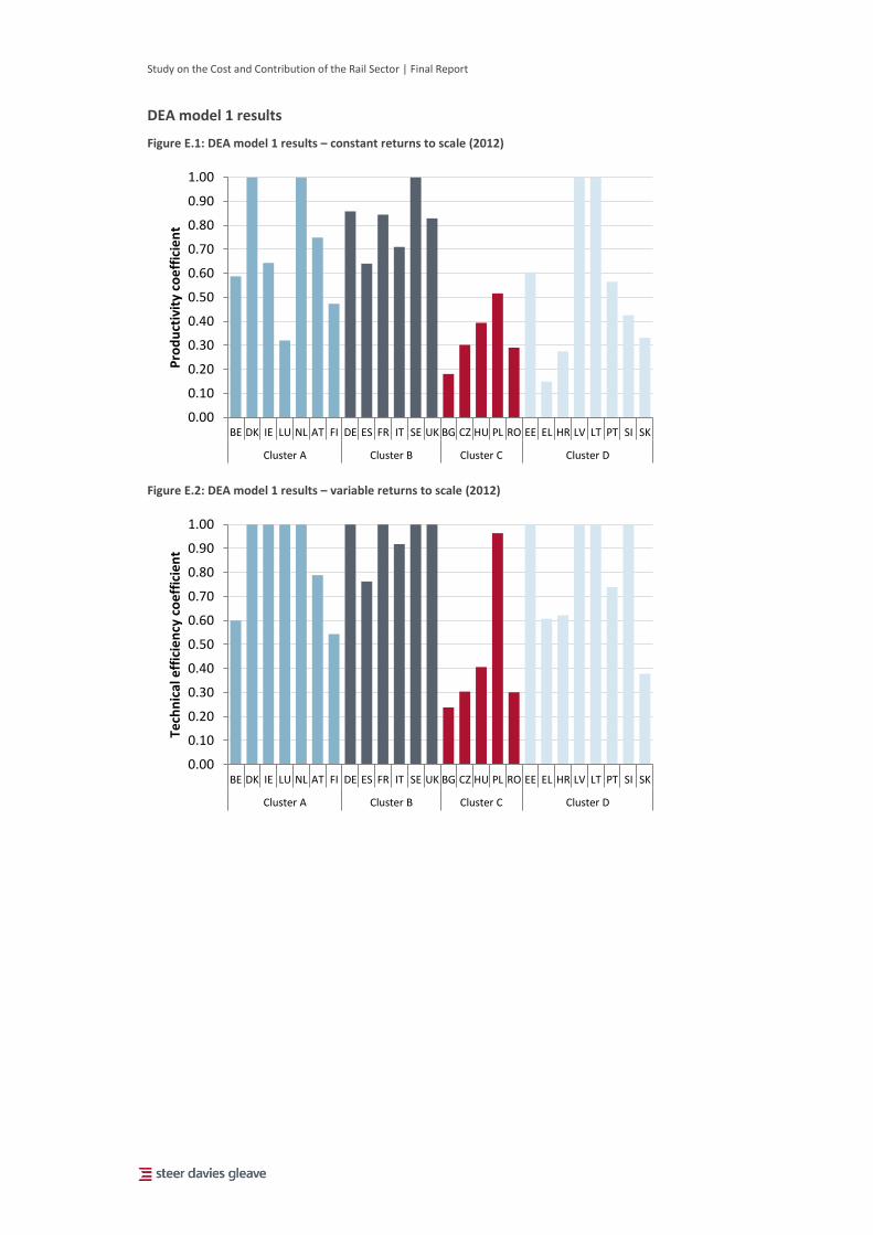
Study on the Cost and Contribution of the Rail Sector | Final Report
DEA model 1 results
Figure E.1: DEA model 1 results – constant returns to scale (2012)
Figure E.2: DEA model 1 results – variable returns to scale (2012)
0.00
0.10
0.20
0.30
0.40
0.50
0.60
0.70
0.80
0.90
1.00
BE DK IE LU NL AT FI DE ES FR IT SE UK BG CZ HU PL RO EE EL HR LV LT PT SI SK
Cluster A Cluster B Cluster C Cluster D
Pro
du
ctiv
ity
coe
ffic
ien
t
0.00
0.10
0.20
0.30
0.40
0.50
0.60
0.70
0.80
0.90
1.00
BE DK IE LU NL AT FI DE ES FR IT SE UK BG CZ HU PL RO EE EL HR LV LT PT SI SK
Cluster A Cluster B Cluster C Cluster D
Tech
nic
al e
ffic
ien
cy c
oe
ffic
ien
t

Study on the Cost and Contribution of the Rail Sector | Final Report
DEA model 2 results
E.2 Model 2 has the same inputs and outputs as Run 1, but is modelled over a 3 year period. This
allows for the comparison of efficiency scores over time as well as across the sample.
Figure E.3: DEA model 2 results – variable returns to scale (2012)
Figure E.4: DEA model 2 results – constant returns to scale over time (sample of Member States)
0.00
0.10
0.20
0.30
0.40
0.50
0.60
0.70
0.80
0.90
1.00
BE DK IE LU NL AT FI DE ES FR IT SE UK BG CZ HU PL RO EE EL HR LV LT PT SI SK
Cluster A Cluster B Cluster C Cluster D
Tech
nic
al e
ffic
ien
cy c
oe
ffic
ien
t
-
0.2
0.4
0.6
0.8
1.0
1.2
2010 2011 2012
Pro
du
ctiv
ity
coe
ffic
ien
t
Year CZ ES IT NL AT PL PT
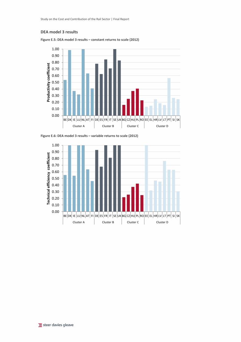
Study on the Cost and Contribution of the Rail Sector | Final Report
DEA model 3 results
Figure E.5: DEA model 3 results – constant returns to scale (2012)
Figure E.6: DEA model 3 results – variable returns to scale (2012)
0.00
0.10
0.20
0.30
0.40
0.50
0.60
0.70
0.80
0.90
1.00
BE DK IE LU NL AT FI DE ES FR IT SE UK BG CZ HU PL RO EE EL HR LV LT PT SI SK
Cluster A Cluster B Cluster C Cluster D
Pro
du
ctiv
ity
coe
ffic
ien
t
0.00
0.10
0.20
0.30
0.40
0.50
0.60
0.70
0.80
0.90
1.00
BE DK IE LU NL AT FI DE ES FR IT SE UK BG CZ HU PL RO EE EL HR LV LT PT SI SK
Cluster A Cluster B Cluster C Cluster D
Tech
nic
al e
ffic
ien
cy c
oe
ffic
ien
t

Study on the Cost and Contribution of the Rail Sector | Final Report
DEA model 4 results
Figure E.7: DEA model 4 results – constant returns to scale (2012)
Figure E.8: DEA model 4 results – variable returns to scale (2012)
0.00
0.10
0.20
0.30
0.40
0.50
0.60
0.70
0.80
0.90
1.00
BE DK IE LU NL AT FI DE ES FR IT SE UK BG CZ HU PL RO EE EL HR LV LT PT SI SK
Cluster A Cluster B Cluster C Cluster D
Pro
du
ctiv
ity
coe
ffic
ien
t
0.00
0.10
0.20
0.30
0.40
0.50
0.60
0.70
0.80
0.90
1.00
BE DK IE LU NL AT FI DE ES FR IT SE UK BG CZ HU PL RO EE EL HR LV LT PT SI SK
Cluster A Cluster B Cluster C Cluster D
Tech
nic
al e
ffic
ien
cy c
oe
ffic
ien
t

Study on the Cost and Contribution of the Rail Sector | Final Report
DEA model 5 results
Figure E.9: DEA model 5 results – constant returns to scale (2012)
Figure E.10: DEA model 5 results – variable returns to scale (2012)
0.00
0.10
0.20
0.30
0.40
0.50
0.60
0.70
0.80
0.90
1.00
BE DK IE LU NL AT FI DE ES FR IT SE UK BG CZ HU PL RO EE EL HR LV LT PT SI SK
Cluster A Cluster B Cluster C Cluster D
Pro
du
ctiv
ity
coe
ffic
ien
t
0.00
0.10
0.20
0.30
0.40
0.50
0.60
0.70
0.80
0.90
1.00
BE DK IE LU NL AT FI DE ES FR IT SE UK BG CZ HU PL RO EE EL HR LV LT PT SI SK
Cluster A Cluster B Cluster C Cluster D
Tech
nic
al e
ffic
ien
cy c
oe
ffic
ien
t
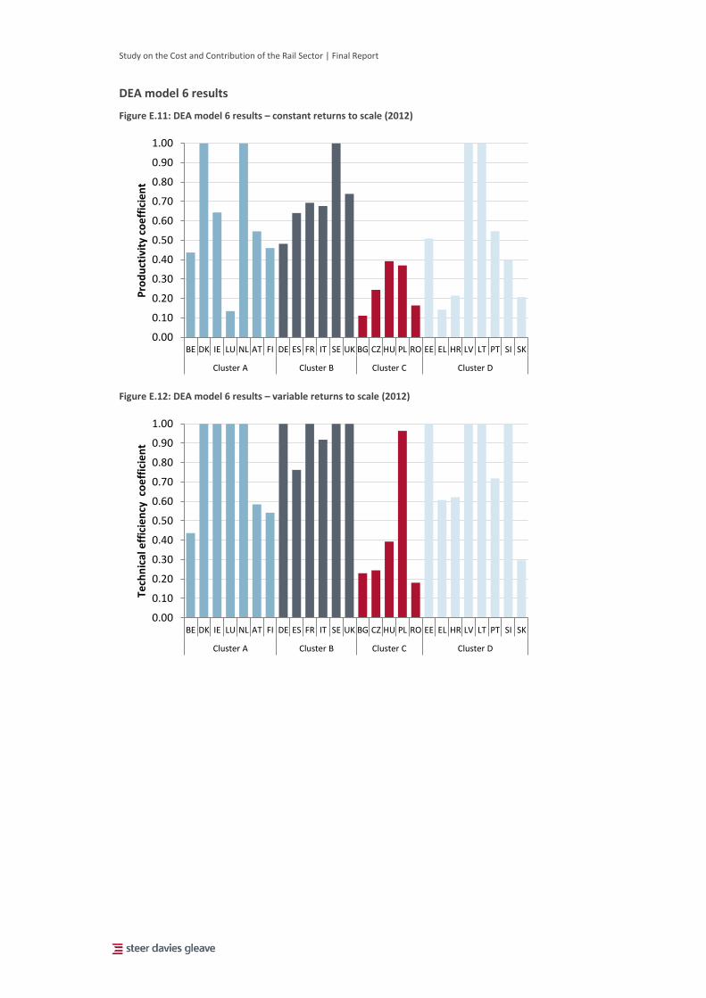
Study on the Cost and Contribution of the Rail Sector | Final Report
DEA model 6 results
Figure E.11: DEA model 6 results – constant returns to scale (2012)
Figure E.12: DEA model 6 results – variable returns to scale (2012)
0.00
0.10
0.20
0.30
0.40
0.50
0.60
0.70
0.80
0.90
1.00
BE DK IE LU NL AT FI DE ES FR IT SE UK BG CZ HU PL RO EE EL HR LV LT PT SI SK
Cluster A Cluster B Cluster C Cluster D
Pro
du
ctiv
ity
coe
ffic
ien
t
0.00
0.10
0.20
0.30
0.40
0.50
0.60
0.70
0.80
0.90
1.00
BE DK IE LU NL AT FI DE ES FR IT SE UK BG CZ HU PL RO EE EL HR LV LT PT SI SK
Cluster A Cluster B Cluster C Cluster D
Tech
nic
al e
ffic
ien
cy c
oe
ffic
ien
t

Study on the Cost and Contribution of the Rail Sector | Final Report
F Scenario modelling tool – record of assumptions Base Case
Outputs
F.1 For all output data, the Reference scenario 2013 results are available for the years 2010, 2015,
2020, 2025, 2030, 2035, 2040, 2045 and 2050. Data between these years has been
interpolated and assumed to grow at a constant rate. Outputs include:
Rail passenger kilometres (the sum of conventional and high speed rail);
Freight rail tonne kilometres;
Road passenger kilometres; and
Road freight tonne kilometres.
Emissions
F.2 For all emissions data, the Reference scenario 2013 results are available for the years 2010,
2015, 2020, 2025, 2030, 2035, 2040, 2045 and 2050. Data between these years has been
interpolated and assumed to grow at a constant rate. Data include:
Rail passenger CO2 emissions;
Freight rail CO2 emissions;
Road passenger CO2 emissions; and
Road freight CO2 emissions;
Rolling Stock
F.3 Passenger rolling stock numbers are taken from the input data gathered from UIC datasets and
national sources for years 2010, 2011, 2012. The figures for subsequent years are based on the
growth rates from the PRIMES-TREMOVE Transport Model ‘stock’ section for ‘Rail Transport-
Passenger’.
F.4 Freight rolling stock numbers are taken from the input data gathered from UIC datasets and
national sources for years 2010, 2011, 2012. The figures for subsequent years are based on the
growth rates from the Reference scenario 2013 results.
Inputs
Track km
F.5 Track km for the years 2010, 2011 and 2012 are taken from the input data gathered from UIC
datasets and the EU Statistical Pocketbook. For subsequent years, track km is assumed to
remain constant at the 2012 level.

Study on the Cost and Contribution of the Rail Sector | Final Report
Operating Costs (Opex)
F.6 Operating costs for the years 2010, 2011 and 2012 are taken from the input data gathered
from UIC datasets and national sources. These costs have been deflated to 2010 prices using
Eurostat Annual average HICP data.
F.7 For subsequent years, operating costs per unit are assumed to remain constant at the average
(mean) value of 2010 – 2012. Total operating costs rise in line with passenger and freight
outputs.
Exogenous Variables
F.8 The exogenous variable data is available for the years 2010, 2015, 2020, 2025, 2030, 2035,
2040, 2045 and 2050 data between these years has been interpolated and assumed to grow at
a constant rate.
GDP data projections is taken from the EPC/ECFIN Ageing Report 2012.
Population data is taken from Eurostat - EUROPOP2010 population projections.
Scenario test
Step one – reduce operating costs
F.9 Based upon the expected efficiency level for a given Member State in a given year (as defined
by its efficiency score and efficiency trajectory), we calculate the operating cost savings that
can be achieved. This results in a reduction in total costs for a given level of output (i.e. unit
costs fall).
F.10 Efficiency savings are assumed to affect freight and passenger rail in equal measure and
therefore cost savings are distributed between the provision of freight and passenger services
according to the share of total costs attributable to delivering freight and passenger services.
Step two – increase output
F.11 The total cost saving achieved in year t (e.g. 2015) is reinvested in year t+1 (e.g. 2016) to
deliver additional passenger and freight outputs. The unit cost for any additional output in
year t+1 is taken from the calculation described in paragraph F.9 for year t50.
F.12 The quantity of additional outputs that can be generated from cost savings is calculated
separately for freight and passenger outputs.
Step three – economic benefits
F.13 By reducing the quantity of inputs needed to deliver a given level of outputs, when considered
in isolation the results of ‘step one’ can be considered as an increase in operating surplus or
value added. Alternatively, they can be thought of as an intermediate baseline against which
the increase in output estimated through ‘step two’ can be compared. By increasing the
outputs delivered by (and therefore expenditure of) the rail sector at a given unit cost, we
would expect there to be second and third-round effects on other sectors of the economy.
50
For example, in the counterfactual scenario Member State A generates outputs of 10 billion passenger kilometres at a cost of €10 million (i.e. 1,000 passenger kilometres/€). In the efficiency scenario, its total costs fall to €8 million in year t. In year t+1 the €2 million saved is re-invested to generate additional rail outputs at the more efficient cost per unit of 1,250 passenger kilometres/€. Output increases by 2.5bn passenger kilometres (€2 million x 1,250 passenger kilometres/€).
Study on the Cost and Contribution of the Rail Sector | Final Report
Therefore, in addition to the direct increase in output and employment within the rail sector,
indirect impacts need to be estimated through output and employment multipliers.
F.14 For those Member States where we have a direct estimate (Austria, Netherlands, Italy, UK ,
Czech Republic, Poland, Portugal, Slovakia), their specific output and employment multipliers
have been applied to the total operating cost savings/additional expenditure. For those
Member States where no direct estimate is available, an arithmetic mean of the multipliers for
those countries in their cluster has been applied.
Step four – externalities
F.15 In order to estimate the net impact of additional rail outputs upon external factors (CO2
emissions, noise and safety) it is necessary to make two assumptions. First, we assume that all
of the additional supply generated by the rail industry is taken up with additional demand i.e.
there is latent demand that is not fulfilled within the counterfactual scenario. Second, we
assume that 20% of all additional rail passenger and freight kilometres are abstracted from the
road network. The scenario assessment calculator has the facility to allow us to amend these
assumptions.
F.16 Finally, using values taken from the Update of the Handbook on External Costs of Transport,
we have calculated the net marginal impact of a reduction in road use (by both freight and
passenger traffic) and a corresponding increase in rail use. For example, the reduction in road
passenger/vehicle kilometres is multiplied by the relevant value of a marginal change in usage
to generate a gross reduction in highway externalities, from which the equivalent value of
externalities generated by an increase in rail passenger/vehicle kilometres is subtracted to
estimate a net overall figure.

Study on the Cost and Contribution of the Rail Sector | Final Report
G Bibliography Publications
2011 White Paper, Roadmap to a Single European Transport Area – Towards a competitive and
resource efficient transport system (European Commission)
Achieving Value for Money from People in the GB Rail Industry – Theme H Benchmarking
(AECOM, ITS Leeds, First Class Partnerships, 2011)
EU Transport in Figures: Statistical Pocketbook 2015 (European Commission)
Fourth Report on Monitoring Development of the Rail Market (European Commission, 2014)
The Economic Footprint of Railway Transport in Europe (CER, 2014)
The economic footprint of railway travel in Europe (CER, 2014)
What is the contribution of rail to the UK economy? (Oxera, 2014)
Books
A guide to DEAP Version 2.1 (Coelli, 1996)
Introduction to Data Mining (Tan, Steinbach and Kumar, 2006)
Papers
Cantos et al (2011), Evaluating European Railway Deregulation Using Different Approaches
Dodgson, J. S. (1986) Benefits of Changes in Urban Public Transport Subsidies in the Major
Australian Cities Economic Record 62, pp.224-235
Dodgson. J (2011), New, Disaggregated, British Railway Total Factor Productivity Growth
Estimates, 1875 to 1912, The Economic History Review v64
Friebel et al (2008), Railroad (De)Regulation – A European Efficiency Comparison, Economica
Friebel, Ivaldi, Vibes (2003), Railway deregulation: A European efficiency comparison,
Economica
Growtisch and Wetzel (2009), Testing for Economies of Scope in European Railways: An
Efficiency Analysis, Working Paper
Laabsch, Sanner (2012), The Impact of Vertical Separation on the Success of the Railways,
European Railway Policy
Merkert et al (2010), Benchmarking of train operating firms – a transaction cost efficiency
analysis, Transportation Planning and Technology
Study on the Cost and Contribution of the Rail Sector | Final Report
Mizutani and Uranishi (2013), Does Vertical Separation Reduce Cost? An Empirical Analysis of
the Rail Industry in European and East Asian OECD Countries, Journal of Regulatory Economics
Mizutani, Uranishi (2010), Does Vertical Separation Reduce Cost?, Journal of Regulatory
Economics
Oum and Yu (1994), Economic efficiency of railways and implications for public policy, Journal
of transport Economics and Policy
Pvlyuk (2008), Efficiency analysis of European countries railways, Proceedings of the 8th
International Conference Reliability and Statistics in Transportation and Communication
Rijkure. A and Sare. I (2013), The Role of Latvian Ports Within Baltic Sea Region, European
Integration Studies, 2013 No 7
Sánchez, Monsálvez and Martínezn (2008), Vertical and Horizontal Separation in the European
Railway Sector: Effects on Productivity, Fundación BBVA
Vassallo, Fagan (2007), Nature or nurture: why do railroads carry greater freight share in the
United States than in Europe?, Transportation
Ward, J.H. (1963) Hierarchical Grouping to Optimize and Objective Function, Journal of the
American Statistical Association
Wardman (2006), Demand for rail travel and the effects of external factors, Transportation
Research Part E: Logistics and Transportation Review
Wetzel (2008), European Railway Deregulation, The influence of regulatory and environmental
conditions on efficiency, Working Paper

steerdaviesgleave.com
e