arX

iv:h

ep-t

h/05

1124

5v1

24

Nov

200

5

On the Hamiltonian reduction of geodesic motion on

SU(3) to SU(3)/SU(2)

V. Gerdt a , R. Horan b , A. Khvedelidze a,b,c , M. Lavelle b ,

D. McMullan b and Yu. Palii a

a Laboratory of Information Technologies,

Joint Institute for Nuclear Research,

Dubna, 141980, Russia

b School of Mathematics and Statistics,

University of Plymouth,

Plymouth, PL4 8AA, United Kingdom

c Department of Theoretical Physics,

A.M.Razmadze Mathematical Institute,

Tbilisi, GE-0193, Georgia

Abstract

The reduced Hamiltonian system on T∗(SU(3)/SU(2)) is derived from a Riemannian geodesic

motion on the SU(3) group manifold parameterised by the generalised Euler angles and endowed

with a bi-invariant metric. Our calculations show that the metric defined by the derived reduced

Hamiltonian flow on the orbit space SU(3)/SU(2) ≃ S5 is not isometric or even geodesically equiv-

alent to the standard Riemannian metric on the five-sphere S5 embedded into R

6.

1

Contents

I. Introduction 3

A. Hamiltonian reduction 4

II. Geodesic flow on SU(2) 6

A. The Euler angle parametrisation 6

B. Quotient SU(2)/U(1) 10

C. Lagrangian in Euler coordinates 11

D. Hamiltonian dynamics on T∗SU(2) 12

E. Hamiltonian reduction to the coset SU(2)/U(1) 13

III. Geodesic flow on SU(3) using generalised Euler coordinates 14

A. Generalised Euler decomposition of SU(3) 14

B. Geometry of the left coset SU(3)/SU(2) 18

C. Lagrangian on SU(3) in terms of generalised Euler angles 21

D. Hamiltonian dynamics on SU(3) 22

E. Hamiltonian reduction to SU(3)/SU(2) 22

IV. Riemannian structures on the quotient space 24

V. Conclusion 25

Acknowledgments 25

A. Appendix 26

1. The su(3) algebra structure 26

2. The basis of invariant 1-forms on the SU(3) group 28

a. The left-invariant 1-forms 28

b. The right-invariant 1-forms 29

3. The basis of the invariant vector fields on the SU(3) group 30

a. The left-invariant vector fields 30

b. The right-invariant vector fields 32

References 35

2

I. INTRODUCTION

Symmetry plays a central role in our pursuit of a better understanding of nature. Through

the preservation or artful breaking of symmetry, powerful models have been developed which

describe the fundamental forces and which have, so far, withstood all tests. Indeed, any

endeavour to go beyond this standard model also has, at its heart, an appropriate symmetry

argument.

An immediate consequence of symmetry is that it permits for a reduction in the relevant

degrees of freedom needed to describe a given problem. In a gauge theory this reduction

implies that not all the degrees of freedom present in the formulation of the theory correspond

to physical degrees of freedom. So, for example, in Quantum Electrodynamics, with its U(1)

gauge symmetry, the potential Aµ, which naively has four degrees of freedom, describes the

photon, which has just two physical degrees of freedom. Understanding how this type of

reduction should best take place and how the process of quantising a system interacts with

the symmetry, has driven many of the important advances in our understanding of gauge

theories [1].

In many cases, the reduction to the true physical degrees of freedom in a field theory

has been fruitfully studied through simpler, finite dimensional systems. In particular, coset

spaces of the form G/H , where G and H are finite dimensional Lie groups, have provided

much insight [2] into how global and topological properties of these configuration spaces can

be encoded into the quantisation process via generalised notions of reduction to the true

degrees of freedom [3].

In all investigations to date, specific details on dynamical aspects of the reduction to G/H

have been restricted to groups for which manageable parameterisations of the group elements

exist. Essentially this has restricted attention to groups directly related to the rotation group

and its covering, SU(2). However, recently there has been much progress in finding suitable

parameterisations for the higher dimensional unitary groups [4, 5, 6, 7] and particularly

for the group SU(3) [8, 9]. These advances open the door to detailed investigations of

dynamics on spaces such as the five-sphere, S5, now viewed as the reduction from SU(3)

to SU(3)/SU(2). By exploiting our concrete description of this reduction we shall see a

new phenomenon for this system: different metric structures emerge depending on whether

the five sphere is viewed as the coset space or via its natural embedding in six dimensional

3

Euclidean space. This is, to the best of our knowledge, the first explicit example of this

metric property of reduction.

The plan of the paper is as follows. We will conclude this introduction with a brief

summary of the classical Hamiltonian reduction procedure. Then, in section 2, we will see

how this procedure is applied to the group SU(2). This section does not contain any new

results, but fixes notation and introduces themes that will prepare us for the reduction

on the configuration space SU(3) which will be presented in detail in section 3. Then, in

section 4 we will investigate the possible Riemannian structures that arise on the quotient

space S5 and discuss the possible metric and geodesic correspondences. In an appendix we

will collect together the details of our consistent parametrisation of SU(3).

A. Hamiltonian reduction

Consider the special class of Lagrangian systems whose configuration space is a compact

matrix Lie group G. This means that the state of a system at fixed time t = 0 is characterised

by an element of the Lie group g(0) ∈ G and the evolution is described by the curve g(t)

on the group manifold [10, 11]. The “free evolution” on the semisimple group G is, by

definition, the Riemannian geodesic motion on the group manifold with respect to the so-

called Cartan-Killing metric [12, 13]

ds2G

= κ Tr(

g−1dg ⊗ g−1dg)

,

where κ is a normalisation factor. The geodesics are given by the extremal curves of the

action functional

S[g] =κ

2

∫ T

0

dt Tr(

g−1g g−1g)

. (1.1)

This action is invariant under the continuous left translation

g(t) → g(ε) g(t) , ε = ( ε1 , ε2 , . . . , εdimG) ,

and therefore the system possesses the integrals of motion I1 , I2 , . . . , IdimG . The existence

of these integrals of motion allows us to reduce the number of degrees of freedom of the

system using the well-known method of Hamiltonian reduction [10, 11].

For a generic Hamiltonian system defined on T ∗M with symmetry associated to the Lie

group G action, the level set of the corresponding integrals of motion

Mc = I−1(c) . (1.2)

4

where c is a set of arbitrary real constants c = (c1 , . . . , cdimG), determines the reduced

Hamiltonian system on the reduced phase space Fc ⊂ Mc. The subset Fc is described by the

isotropy group, Gc , of the integrals level set Mc

Fc = Mc/Gc .

Here we are interested in a special case when the manifold M is itself a group manifold and

the symmetry transformation are group translations. Now the level set Mc is a subset of

the trivial cotangent bundle T ∗G which can be identified with the product of the group G

and its algebra, G × g. The level set given by the integrals I1 = c1 , I2 = c2 , . . . , IN =

cN , N ≤ dim G , defines the isotropy group Gc ⊂ G and the so-called orbit space

O = G/Gc . (1.3)

The relationship between the orbit space O and the reduced phase space Fc can be sum-

marised as follows (see e.g. [10, 11]):

• the reduced phase space Fc is symplectic and diffeomorphic to the cotangent bundle

T∗O;

• the dynamics on the reduced degrees of freedom is Hamiltonian with a reduced Hamil-

tonian given by the projection of the original Hamiltonian function to Fc.

These results are the modern generalisations of the classical theorems proving that the

collection of holonomic constraints defines a configuration manifold M as a submanifold of

Rn and that, in the absence of forces, the trajectories of mechanical system are geodesics of

the induced Riemannian metric.

Note that the above results do not claim that the reduced phase space and the dynamics

on the orbit space are isometric. Indeed, we know that on the reduced phase space we can

define, at least locally, an induced metric that arises from the kinetic energy energy part of

the reduced Hamiltonian

KO =1

2gO(ξa, ξb)pa pb , (1.4)

On the other hand the map π : G → G/Gc induces the metric

gO = π∗gG. (1.5)

We now pose a question about the relation between these two metrics.

5

When are the metrics gO and gO isometrically or, more weakly, geodesically

equivalent?

We do not know the general answer to this question, so in this present note we will focus

our study on two examples: geodesic motion on the SU(2) and SU(3) group manifolds.

We start with a well-known example of Hamiltonian reduction SU(2) → SU(2)/U(1)

and show that the reduced space is indeed in isometrical correspondence with the cotangent

bundle T∗S

2 and the standard induced metric on the two-sphere S2. The case of the SU(3)

→ SU(3)/SU(2) reduction gives an example of the opposite result: the metric defined by

the Hamiltonian flow on on the orbit space SU(3)/SU(2) is not isometrically equivalent

to a standard round metric on the five-sphere S5. Furthermore, in this case, the stronger

result is true: the reduced configuration space and the standard S5 are not even geodesically

equivalent.

II. GEODESIC FLOW ON SU(2)

In this section we discuss the example of reduction of free motion on the SU(2) group

manifold. We start with a presentation of the key geometrical structures found on this group

which are necessary for any further dynamical analysis.

A. The Euler angle parametrisation

The special unitary group SU(2), considered as a subgroup of the general matrix group

GL(2, C), is topologically the three-sphere S3 embedded into C2. This correspondence

SU(2) ≈ S3 follows immediately from the standard identification of an arbitrary element

g ∈ SU(2) as

g :=

z1 −z2

z2 z1

, |z1|2 + |z2|2 = 1 . (2.1)

The three-sphere S3 is a manifold which requires more than one chart to cover it and therefore

there is no global parametrisation of the SU(2) group as a 3-dimensional space. The local

description usually adopted is given by the conventional symmetric Euler representation

[14] for a group element

g = exp(

iα

2σ3

)

exp

(

iβ

2σ2

)

exp(

iγ

2σ3

)

, (2.2)

6

with the appropriately chosen range for the Euler angles α , β , γ .

In this representation the generators of the one-parameter subgroups are the standard

Pauli matrices σ1 , σ2 and σ3 ,

σ1 =

0 1

1 0

, σ2 =

0 −i

i 0

, σ3 =

1 0

0 −1

, (2.3)

satisfying the su(2) algebra

σaσb − σbσa = 2 i ǫabc σc . (2.4)

Writing the complex numbers in (2.1) as z1 = x1 + ix2 and z2 = x3 + ix4 in polar form

z1 := eiu cos θ , z2 := eiv sin θ , (2.5)

and comparing (2.1) with the explicit form of the Euler matrix (2.2)

g =

eiα + γ

2 cos

(

β

2

)

eiα − γ

2 sin

(

β

2

)

−e−i

α − γ

2 sin

(

β

2

)

e−i

α + γ

2 cos

(

β

2

)

, (2.6)

we have

u =α + γ

2, v =

α − γ

2, θ =

β

2. (2.7)

The Euler decomposition (2.2) corresponds to the following parametric representation of the

three-sphere embedded in R4:

x1 = cos

(

α + γ

2

)

cos

(

β

2

)

, x2 = sin

(

α + γ

2

)

cos

(

β

2

)

,

x3 = − cos

(

α − γ

2

)

sin

(

β

2

)

, x4 = sin

(

α − γ

2

)

sin

(

β

2

)

.

(2.8)

To be more precise, though, this is not a valid parametrisation for the entire three-sphere.

In particular, the neighbourhood of the identity element of the group in this decomposition

turns out to be degenerate. The identity element of SU(2) corresponds to the whole set:

β = 0 and α+γ = 0 . In order to properly cover the whole group manifold it is necessary to

consider an atlas on the SU(2) group and used different parameterisations on the different

charts. Bearing this in mind, we proceed by assuming that we are working in a chart (U , φ)

7

where α , β and γ serve as good local coordinates on S3 and calculate the Maurer-Cartan

forms on SU(2).

Using the following normalisation

g−1dg =i

2

3∑

a = 1

σa ⊗ ωaL , (2.9)

dg g−1 =i

2

3∑

a = 1

σa ⊗ ωaR (2.10)

and performing the straightforward calculations with the Eulerian representation (2.2) we

arrive at the well-known expressions for left-invariant 1-forms

ω1L = cos γ sin β dα − sin γ dβ ,

ω2L = sin β sin γ dα + cos γ dβ , (2.11)

ω3L = cos β dα + dγ .

and the corresponding dual vectors, ωaL( XL

b ) = δab , a, b = 1 , 2 , 3 ,

XL1 =

cos γ

sin β

∂

∂α− sin γ

∂

∂β− cot β cos γ

∂

∂γ,

XL2 =

sin γ

sin β

∂

∂α+ cos γ

∂

∂β− cot β sin γ

∂

∂γ, (2.12)

XL3 =

∂

∂γ.

The right invariant 1-forms and the corresponding dual vectors, ωaR( XR

b ) = δab , are

ω1R = sin α dβ − cos α sin β dγ ,

ω2R = cos α dβ + sin α sin β dγ , (2.13)

ω3R = dα + cos β dγ .

XR1 = cos α cot β

∂

∂α+ sin α

∂

∂β− cos α

sin β

∂

∂γ,

XR2 = − sin α cotβ

∂

∂α+ cos α

∂

∂β+

sin α

sin β

∂

∂γ, (2.14)

XR3 =

∂

∂α.

The vector fields XLa and XR

a obey the su(2)⊗su(2) algebra with respect to the Lie brackets

8

operation

[

XLa , XL

b

]

= −ǫabc XLc (2.15)

[

XRa , XR

b

]

= ǫabc XRc (2.16)

[

XLa , XR

b

]

= 0 . (2.17)

Any compact Lie group can be endowed with the bi-invariant Riemannian metric build

uniquely (up to a normalization factor) from the Cartan-Killing form over the algebra. It

is convenient to choose the following normalization for the bi-invariant metric on the SU(2)

group:

gSU(2)

= −1

2Tr(

g−1dg ⊗ g−1dg)

. (2.18)

In terms of this left/right-invariant non-holonomic frame, (2.18) reads

gSU(2)

=1

4

(

ω1L ⊗ ω1

L + ω2L ⊗ ω2

L + ω3L ⊗ ω3

L

)

, (2.19)

=1

4

(

ω1R ⊗ ω1

R + ω2R ⊗ ω2

R + ω3R ⊗ ω3

R

)

. (2.20)

Substitution of the expressions (2.11) and (2.13) for the Maurer-Cartan forms ωL and ωR

yields the metric in the coordinate frame dα , dβ , dγ basis

gSU(2)

=1

4(dα ⊗ dα + dβ ⊗ dβ + dγ ⊗ dγ + 2 cosβ dα ⊗ dγ) . (2.21)

In order to understand the metrical characteristics of a group manifold viewed as an embed-

ded space, it is instructive to compare this invariant metric with the metric induced from

the ambient 4-dimensional Euclidian space on the unit three-sphere (2.8)

gS3

= dz1 ⊗ dz1 + dz2 ⊗ dz2 (2.22)

=1

4(dα ⊗ dα + dβ ⊗ dβ + dγ ⊗ dγ + 2 cosβdα ⊗ dγ) .

Comparing the metrics, (2.21) and (2.22), we conclude that the bi-invariant metric on SU(2)

is the same as the standard metric on the unit three-sphere S3 and its bi-invariant volume

is

Vol(SU(2)) =

∫

√

det gSU(2)

dα ∧ dβ ∧ dγ

=

(

1

2

)3 ∫ 2π

0

dα

∫ 4π

0

dγ

∫ π

0

dβ sin(β) = 2π2 = Vol( S3) . (2.23)

9

As a Riemannian manifold the SU(2) group endowed with the metric (2.21) is a 3-

dimensional space of constant curvature with the Riemann scalar RSU(2)

= 6 and the Ricci

tensor Rab given by

Rab =R

SU(2)

3gab = 2 gab . (2.24)

The Gaussian curvature K of an n-dimensional manifold and the Riemann scalar are related

via

K =R

n(n − 1), (2.25)

therefore KSU(2) = 1 in agreement with the volume calculation (2.23).

B. Quotient SU(2)/U(1)

Here we recall the key ingredients of the construction of a quotient space G/H by con-

sidering the transitive action of the group G on a certain base space M . We have the result

that [27]:

If the group G acts transitively on a set M with H ⊂ G being an isotropy subgroup

leaving a point x0 ∈ M fixed

H = {g ∈ G | g · x0 = x0} ,

then the set M is in one-to-one correspondence with the left cosets gH of G .

The explicit form of this map for the SU(2) group is as follows. We identify the su(2)

algebra with R3 by the map, xa ∈ R3 → X ∈ su(2)

X =3∑

a=1

xaσa . (2.26)

Consider now the adjoint action of SU(2) on an element of its algebra X ∈ su(2)

Ad(g)(X) = g X g−1 .

The base point x0 = (0 , 0 , 1) (corresponding to the element σ3) has a one-parameter isotropy

subgroup

H = exp(

iα

2σ3

)

.

10

The orbit space of σ3

Ad(g)(σ3) = g σ3 g−1 ,

is the coset SU(2)/U(1). The proper atlas covering the SU(2) group manifold provides the

coset space parametrisation. When SU(2) ≃ S3 is parameterised in terms of two complex

coordinates z1 and z2 and the two-sphere is described by a unit vector n = (n1 , n2 , n3), then

the projection S3 → S

2 reads explicitly

(z1, z2) → (n1 , n2 , n3) =(

2ℜ[z1z2] , 2ℑ[z1z2] , |z1|2 − |z2|2)

. (2.27)

This is the famous Hopf projection map π : SU(2) → S2 showing that SU(2) is a fibre

bundle over S2 with nonintersecting circles U(1) ≡ S1 as fibres

S1 → SU(2)

π→ S2 .

Using the Euler decomposition (2.6) the coset parametrisation reads

g σ3 g−1 = na σa , (2.28)

with the unit 3-vector

n = (− sin β cos α , sin β sin α , cos β ) . (2.29)

C. Lagrangian in Euler coordinates

The bi-invariant Lagrangian

LSU(2) = −1

2Tr

(

g−1(t)d

dtg(t) g−1(t)

d

dtg(t)

)

, (2.30)

in terms of left/right invariant Maurer-Cartan forms (2.9) reads

LSU(2) =1

4

3∑

a=1

iUωaL iUωa

L

=1

4

3∑

a=1

iUωaR iUωa

R , (2.31)

where iU is the interior contraction of the vector field U = α ∂∂α

+ β ∂∂β

+ γ ∂∂γ

.

Covering the group manifold with an atlas and considering the chart where the parameters

α, β, γ in the Euler decomposition (2.2) serve as good coordinates, we arrive at

LSU(2) =1

4

(

α2 + β2 + γ2 + 2 cos(β)αγ)

. (2.32)

11

Comparing (2.32) with the expression (2.21) for the bi-invariant metric on SU(2) we conclude

that

LSU(2) = gSU(2)

(U , U) . (2.33)

D. Hamiltonian dynamics on T∗SU(2)

The Hamiltonian dynamics on the SU(2) group is defined on the cotangent bundle

T∗SU(2) which can be identified with the trivialisation T∗SU(2) ≈ SU(2) × su(2)L or with

T∗SU(2) ≈ SU(2) × su(2)R .

The canonical Hamiltonian describing geodesic motion on SU(2) can be obtained by a

Legendre transformation of the Lagrangian function (2.31). Introducing the Poincare-Cartan

symplectic one-form

Θ = pα dα + pβ dβ + pγ dγ ,

with the canonically conjugated pairs

{α , pα} = 1 , {β , pβ} = 1 , {γ , pγ} = 1 ,

the Hamiltonian on T∗SU(2) is defined as

HSU(2) =3∑

a=1

ξLa ξL

a ,

=3∑

a=1

ξRa ξR

a , (2.34)

where ξLa and ξR

a are the values of the one-form Θ on the left/right invariant vector fields

XLa , XR

a spanning the algebra su(2)L,R

ξLa := Θ

(

XLa

)

ξRa := Θ

(

XRa

)

.

The set of functions ξLa and ξR

a obey the su(2)L × su(2)R relations with respect to the

Poisson brackets

{ξLa , ξL

b } = −ǫabc ξLc (2.35)

{ξRa , ξR

b } = ǫabc ξRc (2.36)

{ξLa , ξR

b } = 0 . (2.37)

12

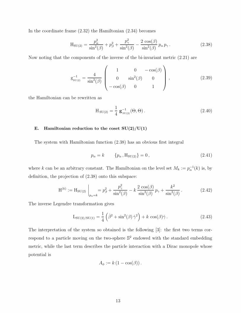
In the coordinate frame (2.32) the Hamiltonian (2.34) becomes

HSU(2) =p2

α

sin2(β)+ p2

β +p2

γ

sin2(β)− 2 cos(β)

sin2(β)pα pγ . (2.38)

Now noting that the components of the inverse of the bi-invariant metric (2.21) are

g−1SU(2)

=4

sin2(β)

1 0 − cos(β)

0 sin2(β) 0

− cos(β) 0 1

, (2.39)

the Hamiltonian can be rewritten as

H SU(2) =1

4g−1

SU(2)(Θ, Θ) . (2.40)

E. Hamiltonian reduction to the coset SU(2)/U(1)

The system with Hamiltonian function (2.38) has an obvious first integral

pα = k {pα , HSU(2)} = 0 , (2.41)

where k can be an arbitrary constant. The Hamiltonian on the level set Mk := p−1α (k) is, by

definition, the projection of (2.38) onto this subspace:

H(k) := HSU(2)

∣

∣

∣

∣

pα=k

= p2β +

p2γ

sin2(β)− k

2 cos(β)

sin2(β)pγ +

k2

sin2(β). (2.42)

The inverse Legendre transformation gives

LSU(2)/SU(1) =1

4

(

β2 + sin2(β) γ2)

+ k cos(β)γ . (2.43)

The interpretation of the system so obtained is the following [3]: the first two terms cor-

respond to a particle moving on the two-sphere S2 endowed with the standard embedding

metric, while the last term describes the particle interaction with a Dirac monopole whose

potential is

Aφ := k (1 − cos(β)) .

13

III. GEODESIC FLOW ON SU(3) USING GENERALISED EULER COORDI-

NATES

A. Generalised Euler decomposition of SU(3)

Now we pass on to the description of the Euler decomposition of the SU(3) group element.

The Euler angle parametrisation of the 3-dimensional rotation group has been generalised

for the higher orthogonal SO(n) and special unitary SU(n) groups [5, 6, 7], [15], [16] and

[17]. Special attention has been paid to the study of the SU(3) [18, 19, 20, 21] and SU(4)

[4] groups.

The starting point for the derivation [28] of the Euler angle representation of the SU(3)

group is the so-called Cartan decomposition which holds for a real semi-simple Lie algebra

G. A decomposition of the algebra G into the direct sum of vector spaces K and P

G = K ⊕ P (3.1)

is a Cartan decomposition of the algebra G if

[K,K] ⊂ K , (3.2)

[K,P] ⊂ P , (3.3)

[P,P] ⊂ K . (3.4)

The Cartan decomposition for a Lie algebra induces a corresponding Cartan decomposi-

tion of the group G

G = KP , (3.5)

where K is a Lie subgroup of G with Lie algebra K and P is given by the exponential map

P = exp(P) .

An explicit realisation of the Cartan decomposition for SU(3) can be achieved using the

standard traceless 3 × 3 Hermitian Gell-Mann matrices λa , (a = 1 , . . . , 8) (the explicit

form of the λ matrices is given in Appendix A1). Indeed, from the expressions for the

commutation relations

[λa, λb] = 2i

8∑

c=1

fabc λc , (3.6)

14

where the structure constants fabc are antisymmetric in all indices and have the non-zero

values

f123 = 1,

f147 = f246 = f257 = f345 = f516 = f637 = 1/2,

f458 = f678 =√

3/2,

(3.7)

it follows that the set of matrices (λ1 , λ2 , λ3 , λ8 ) can be used as the basis for the vector

space K while the matrices (λ4 , λ5 , λ6 , λ7 ) span the Cartan subspace P. Noting that the

set of matrices (λ1, λ2 , λ3 , λ8 ) comprise the generators (λ1 , λ2 , λ3 ) of the SU(2) group, one

can locally represent K as the product of the SU(2) subgroup and a one-parameter subgroup

K = SU(2) eiφλ8 . (3.8)

The second factor, P = exp(P) in the Cartan decomposition (3.5) can be represented as

a product of one-parameter subgroups. Moreover, based on the algebra (3.6), it can be

represented as a product of a one-parameter subgroup generated by an element [29] from

λ4 , . . . , λ7 “sandwiched” between two different copies of K. Fixing this generator to be,

say, λ4, we have

P = K ′ eiθ′λ4 K ′′ . (3.9)

Now observing that [λ8 , λ4] = i√

3λ5, the product KP can be reduced to

G = SU(2) eiθλ5 SU(2)′ eiφλ8 . (3.10)

Therefore, finally choosing the Euler representation for the elements of two subgroups U ∈SU(2) and V ∈ SU(2)′ in terms of two sets of angles (α, β, γ) and (a, b, c)

U(α, β, γ) = exp(

iα

2λ3

)

exp

(

iβ

2λ2

)

exp(

iγ

2λ3

)

, (3.11)

V (a, b, c) = exp(

ia

2λ3

)

exp

(

ib

2λ2

)

exp(

ic

2λ3

)

, (3.12)

we arrive at the generalised Euler decomposition of an element of g ∈ SU(3)

g = U(α, β, γ) Z(θ, φ) V (a, b, c), (3.13)

with

Z(θ, φ) := ei θ λ5 ei φ λ8 . (3.14)

15

Now it is necessary to fix the range of angles in (3.13). Just as in the case of the SU(2) group

where the Euler parametrisation was not a global one, the SU(3) group manifold cannot be

covered by one chart. However there is a range of parameters such that the parametrisation

covers almost the whole manifold except the set whose measure in the integral quantities,

e.g. such as the invariant volume, is zero. The following ranges for the angles in (3.13)

0 ≤ α, a ≤ 2π , 0 ≤ β , b ≤ π , 0 ≤ γ , c ≤ 4π , (3.15)

0 ≤ θ ≤ π

2, 0 ≤ φ ≤

√3π , (3.16)

lead to the invariant volume for SU(3)

Vol(SU(3)) =

∫

SU(3)

∗1 =√

3π5 . (3.17)

Below this result will be checked by an explicit calculation of the volume of the SU(3)

manifold considered as the Riemannian space endowed with the bi-invariant metric

gSU(3)

= −1

2Tr(

g−1 dg ⊗ g−1 dg)

. (3.18)

In terms of the non-holonomic frame built up from the left/right-invariant forms

g−1dg =i

2

8∑

A = 1

λA ⊗ ωAL , (3.19)

dg g−1 =i

2

8∑

A = 1

λA ⊗ ωAR , (3.20)

the Cartan-Killing metric (3.18) has the diagonal form

gSU(3)

=1

4

(

ω1L ⊗ ω1

L + ω2L ⊗ ω2

L + . . . + ω8L ⊗ ω8

L

)

(3.21)

=1

4

(

ω1R ⊗ ω1

R + ω2R ⊗ ω2

R + . . . + ω8R ⊗ ω8

R

)

, (3.22)

while in the corresponding coordinate frame, with the Eulerian coordinates

16

(α , β , γ , a , b , c , θ , φ ), presented in Appendix A.2, it becomes

gSU(3)

=1

4

(

dα ⊗ dα + dβ ⊗ dβ + dγ ⊗ dγ + 2 cos β dα ⊗ dγ)

+1

4

(

da ⊗ da + db ⊗ db + dc ⊗ dc + 2 cos b da ⊗ dc)

+1

2cos θ

[

sin(a + γ)(

sin β dα ⊗ db + sin b dβ ⊗ dc)

(3.23)

+ cos(a + γ)(

dβ ⊗ db − sin β sin b dα ⊗ dc)

]

−√

3

2sin2 θ

(

cos β dα + dγ)

⊗ dφ

+1

4(1 + cos2 θ)

(

cos β dα + dγ)

⊗(

da + cos b dc)

+ dθ ⊗ dθ + dφ ⊗ dφ .

Fixing the range of the Euler angles according to (3.15) and noting that the determinant of

the Cartan- Killing metric (3.23) is

det gSU(3)

=

(

1

2

)12

sin6(θ) cos2(θ) sin2(β) sin2(b) ,

one can check that the group invariant volume on SU(3) agrees with (3.17)

Vol(SU(3)) =

∫

SU(3)

√

det gSU(3)

dα ∧ dβ ∧ dγ ∧ dθ ∧ da ∧ db ∧ dc ∧ dφ

=

(

1

2

)6 ∫ 2π

0

dα

∫ 4π

0

dγ

∫ 2π

0

da

∫ 4π

0

dc

∫

√3π

0

dφ (3.24)

×∫ π

0

dβ sin(β)

∫ π/2

0

dθ cos(θ) sin3(θ)

∫ π

0

db sin(b) =√

3π5 .

This volume is in accordance with the general formula established by I.G. Macdonald in [23]

and expresses the volume element of a compact Lie group in terms of the product of volume

elements of odd-dimensional unit spheres

Vol(SU(3)) =

√3

2× Vol(S5) × Vol(S3) =

√3

2× π3 × 2π2 . (3.25)

In (3.25) the multiplier√

3/2 , comes from the volume of the maximal torus in SU(3),

interpreted sometimes as the “stretching” factor [24, 25]. This fact explicitly shows that the

SU(3) group is not a trivial product of the two spheres, S3 and S5.

The SU(3) group endowed with the bi-invariant metric (3.23) has a constant positive

Riemann scalar curvature

RSU(3) = 24 ,

17

and the Ricci tensor obeys the relations [30]

Rµν =RSU(3)

8gµν = 3 gµν . (3.26)

B. Geometry of the left coset SU(3)/SU(2)

The group SU(3) can be viewed as a principal bundle over the base S5 with the structure

group SU(2)

SU(2) → SU(3)π→ S

5 ,

with the canonical projection π from the SU(3) onto the left coset SU(3)/SU(2) ≃ S5 . This

map can be realised in the following manner. Consider the general linear group GL(3, C).

An arbitrary element M3×3 can be written in the block form

M3×3 =

z3

M2×2 z2

y1 y2 z1

=

aM2×2

b z1

, (3.27)

for complex 2×2 matrix M2×2 and z1 , z2 , z3 , y1 , y2 ∈ C . The U(3) subgroup of the GL(3, C)

group is defined by the two matrix equations

M3×3M†3×3 = I3×3 , M†

3×3M3×3 = I3×3 . (3.28)

When M3×3 is represented in block form, (3.27), the conditions (3.28) reduce to the quadratic

equations

|z1|2 + |z2|2 + |z3|2 = 1 , (3.29)

|z1|2 + |y1|2 + |y2|2 = 1 , (3.30)

and to the set of 2 × 2 matrix equations

M2×2M†2×2 + aa† = I2×2 (3.31)

M†2×2M2×2 + b†b = I2×2 (3.32)

z1 a + M2×2a = 0 (3.33)

z1 b + M†2×2b = 0 . (3.34)

18

Now let S5 be the five-sphere characterised by a unit complex vector Z := (z1 , z2 , z3)T

Z†Z = 1 .

The SU(3) group element g then acts on this through left translations:

Z → Z′ = gZ . (3.35)

Let Z0 be the base point on this five-sphere with coordinates Z0 = (0, 0, 1)T whose isotropy

group is

H3×3 =

0SU(2)

0 1

. (3.36)

Then the coset SU(3)/SU(2) can be identified with the orbit

Z = g · (0 , 0 , 1)T . (3.37)

Using the explicit form of the representation (3.13), the subgroup SU(2) is embedded into

SU(3) as follows:

SU(2) → SU(3) , V =

e−i

a + c

2 cos

(

b

2

)

−e−i

a − c

2 sin

(

b

2

)

0

eia − c

2 sin

(

b

2

)

eia + c

2 cos

(

b

2

)

0

0 0 1

. (3.38)

So the parametrisation of a group element is

g = U Z V = W V ,

where the factor W reads

W =

cos θ cosβ

2ei(u +

1√3φ)

sinβ

2ei(v +

1√3φ)

sin θ cosβ

2ei(u − 2√

3φ)

− cos θ sinβ

2e−i(v − 1√

3φ)

cosβ

2e−i(u − 1√

3φ)

− sin θ sinβ

2e−i(v +

2√3φ)

− sin θ e

i√3φ

0 cos θ e−i

2√3φ

.

19

u =α + γ

2, v =

α − γ

2.

Using these representations in (3.37) we easily identify the projection onto the left coset as

a five-sphere:

π : g ∈ SU(3) → (z1 , z2 , z3) ∈ S5 ,

which explicitly reads

z1 = cos θ e−i

2√3

φ, (3.39)

z2 = − sin θ sinβ

2e− i

2(α − γ +

4√3

φ), (3.40)

z3 = sin θ cosβ

2e

i

2(α + γ − 4√

3φ)

. (3.41)

Under this projection the Euclidean metric tr(dMdM †) on GL(3,C) induces the following

metric on a unit S5

gS5

= dz1 ⊗ dz1 + dz2 ⊗ dz2 + dz3 ⊗ dz3 (3.42)

= sin2 θ

(

1

4

(

dα ⊗ dα + dβ ⊗ dβ + dγ ⊗ dγ + 2 cos β dα ⊗ dγ)

− 2√3

(cos βdα + dγ) ⊗ dφ

)

+ dθ ⊗ dθ +4

3dφ ⊗ dφ ,

whose determinant is

det gS5

=1

48sin6(θ) cos2(θ) sin2(β) . (3.43)

The metric (3.42) defines a unit five-sphere S5 as a constant curvature Riemann manifold

RS5 = 20 , (3.44)

which is in accordance with its Gaussian curvature

KS5 =RS5

5(5 − 1)= 1 ,

as well as with its volume

Vol(S5) =

∫

S5

√

det gS5

dα ∧ dβ ∧ dγ ∧ dθ ∧ dφ (3.45)

=1

4√

3

∫ 2π

0

dα

∫ 4π

0

dγ

∫

√3π

0

dφ

∫ π

0

dβ sin(β)

∫ π/2

0

dθ cos(θ) sin3(θ) = π3 .

20

C. Lagrangian on SU(3) in terms of generalised Euler angles

Consider the Lagrangian describing the geodesic motion on the SU(3) group manifold

with respect to the bi-invariant metric (3.18)

LSU(3) = −1

2Tr

(

g−1(t)d

dtg(t) g−1(t)

d

dtg(t)

)

. (3.46)

Using the generalised Euler angles on SU(3) as the configuration space coordinates and

(3.23) for the bi-invariant metric, one can write the Lagrangian (3.46) as

LSU(3) =1

4

(

α2 + β2 + γ2 + 2 cosβ αγ + a2 + b2 + c2 + 2 cos b ac)

(3.47)

+1

2cos θ

(

sin(a + γ)(

sin β αb + sin b βc)

+ cos(a + γ)(

βb − sin β sin b αc)

)

−√

3

2sin2 θ

(

cos β α + γ)

φ +1

4(1 + cos2 θ)

(

cos β α + γ)(

a + cos b c)

+ θ2 + φ2 .

From this expression and (3.23) for it follows that

LSU(3) = gSU(3)

(Z, Z) . (3.48)

where Z is the vector field on the tangent bundle TSU(3)

Z = α∂

∂α+ β

∂

∂β+ γ

∂

∂γ+ θ

∂

∂θ+ φ

∂

∂φ+ a

∂

∂a+ b

∂

∂b+ c

∂

∂c. (3.49)

It is worth to note that the Euler decomposition (3.13) for elements of SU(3) in terms of

the SU(2) subgroups,

SU(3) = U(α, β, γ) exp(i θ λ5) V (a, b, c) exp(i φ λ8) ,

allows for the expression of the SU(3) Lagrangian (3.47) in terms of the corresponding left

and right invariant elements of the SU(2) Maurer-Cartan 1-forms:

LSU(3) =1

4

3∑

a=1

iUωaL iUωa

L +1

4

3∑

a=1

iV ωaL iV ωa

L

+1

2cos θ

2∑

a=1

iUωaL iV ωi

R − 1

4(1 + cos2 θ) iUω3

L iV ω3R

−√

3

2sin2 θ iUω3

L φ + θ2 + φ2 . (3.50)

Here iU and iV denote the interior contraction of the vector field on each copy of the SU(2)

group, U and V respectively

U = α∂

∂α+ β

∂

∂β+ γ

∂

∂γ, V = a

∂

∂a+ b

∂

∂b+ c

∂

∂c. (3.51)

21

D. Hamiltonian dynamics on SU(3)

Performing the Legendre transformation, we derive the canonical Hamiltonian generating

the dynamics on the SU(3) group manifold:

HSU(3) =1

sin2 θ

[

p2α

sin2 β+ p2

β +

(

tan2 θ +1

sin2 β

)

p2γ − 2

cos β

sin2 βpαpγ (3.52)

+ sin2 θ

(

1 +1

4cot2 θ +

1

sin2 b

)

p2a + p2

b +1

sin2 bp2

c − 2cos b

sin2 bpapc

]

+ 2cos θ

sin2 θ sin β sin b

[

cos(a + γ)

(

(pα − cos β pγ)(pc − cos b pa) − sin b pβ pb

)

− sin(a + γ)

(

sin b(pα − cos β pγ)pb + sin β(pc − cos b pa)pβ

)]

+1

4p2

θ +1

16

(

1 +3

cos2 θ

)

p2φ +

√3

2

pγpφ

cos2 θ−

√3

4

(

1 +1

cos2 θ

)

papφ .

The Hamiltonian (3.52) can be rewritten in a compact form using the left and right-invariant

vector fields on the two SU(2) group copies, U and V used in the Euler decomposition (3.13):

HSU(3) =

3∑

a=1

ζRa ζR

a +1

sin2 θ

2∑

a=1

(ξLa − cos θ ζR

a )2

+1

sin2 2 θ(2 ξL

3 − (1 + cos2 θ) ζR3 −

√3

2sin2 θ pφ)2 +

1

4p2

θ +1

4p2

φ . (3.53)

Here ξLa and ζR

a are functions defined through the relations

ξLa := Θ

(

XLa

)

, ζRa := Θ

(

Y Ra

)

,

with the SU(2) left-invariant vector fields XLa on the tangent space to the U subgroup, TU ,

and the right-invariant fields Y Ra on TV correspondingly.

E. Hamiltonian reduction to SU(3)/SU(2)

The representation (3.53) is very convenient for performing the reduction in degrees of

freedom associated with the SU(2) symmetry transformation. Due to the algebra of Poisson

brackets (2.35) the functions ζL1 , ζL

2 and ζL3 are the first integrals

{ζLa , HSU(3)} = 0 .

Let us consider the zero level of these integrals

ζL1 = 0 , ζL

2 = 0 , ζL3 = 0 . (3.54)

22

Noting the relation between the left and right invariant vector fields on a group one can

express the functions ζRa entering in the Hamiltonian as

ζRc = Ad(V)cb ζL

b ,

where Ad(V)cb is an adjoint matrix of an element V ∈ SU(2). From this one can immediately

find the reduced Hamiltonian on the integral level (3.54). Indeed, projecting the expression

(3.53) on ζRa = 0 we find

HSU(3)/SU(2) =1

sin2 θ

3∑

a=1

ξLa ξL

a +1

sin2 2 θ(2 ξL

3 −√

3

2sin2 θ pφ)

2 +1

4p2

θ +1

4p2

φ , (3.55)

or more explicitly in terms of the canonical coordinates

HSU(3)/SU(2) =1

sin2 θ

(

p2α

sin2 β+ p2

β +

(

tan2 θ +1

sin2 β

)

p2γ − 2

cos β

sin2 βpαpγ +

√3

2tan2 θ pγpφ

)

+1

4p2

θ +1

16

(

1 +3

cos2 θ

)

p2φ . (3.56)

Performing the inverse Legendre transformation we find the Lagrangian

LSU(3)/SU(2) =1

4sin2 θ

(

(

1 − 1

4cos2 β sin2 θ

)

α2 + β2 +1

4

(

3 + cos2 θ)

γ2

+1

2cos β

(

3 + cos2 θ)

αγ − 2√

3 (cos β α + γ)φ

)

+ θ2 + φ2 . (3.57)

Now one can consider the bilinear form (3.57) as the metric gO on the orbit space O =

SU(3)/SU(2)

gO =1

4sin2 θ

(

(

1 − 1

4cos2 β sin2 θ

)

dα ⊗ dα + dβ ⊗ dβ +1

4

(

3 + cos2 θ)

dγ ⊗ dγ (3.58)

+1

2cos β

(

3 + cos2 θ)

dα ⊗ dγ − 2√

3 (cos β dα + dγ) ⊗ dφ

)

+ dθ ⊗ dθ + dφ ⊗ dφ .

Using our previous calculations (3.45) of Vol(S5) with respect to the metric (3.42) induced

by the canonical projection to the left coset π : SU(3) → SU(3)/SU(2) and noting that the

determinant of the new orbit metric (3.58) induced by the Hamiltonian reduction is

det gO =1

64sin6(θ) cos2(θ) sin2(β) , (3.59)

we find

Vol(SU(3)/SU(2)) =

√3

2Vol(S5) , (3.60)

with the same stretching factor√

3/2 as found in (3.25) for the bi-invariant volume of the

SU(3) group.

23

IV. RIEMANNIAN STRUCTURES ON THE QUOTIENT SPACE

Now we are ready to answer the questions about the relation between metric (3.42)

induced on the left coset SU(3)/SU(2) by canonical projection from the ambient Euclidian

space and the metric (3.58) obtained as a result of performing the Hamiltonian reduction of

the geodesic motion from SU(3) to SU(3)/SU(2).

Performing a straightforward calculation of the Riemannian curvature with respect to

the metric (3.58) yields

R(

gSU(3)SU(2)

)

= 21 , (4.1)

while, from the embedding argumentation we used before, the Riemann scalar of the unit

five-sphere S5 with standard metric induced from the Euclidean space is

R(

gS5

)

= 20 . (4.2)

Furthermore, even though the Riemann scalar is a constant, calculations shows that the

metric (3.57) is not the metric of a space of constant curvature.

So, we have found that the Lagrangian of the reduced system defines local flows on the

configuration space which are not isometric to those on S5 with its standard round metric.

We have shown above that the orbit space SU(3)/SU(2) considered as a Riemannian

space with metric g induced from the Cartan-Killing metric on SU(3) is not isometric to the

S5 with the standard round metric g S5 . The next natural question is whether the metrics g

and g S5 are geodesically /projectively equivalent.

There are several criteria on metrics to be geodesically equivalent. According to L.P.

Eisenhart [26], two metrics g and g on n-dimensional Riemann manifold are geodesically

equivalent if and only if

2 (n + 1)∇i(g) gjk = 2gjk ∂iΛ + gik ∂jΛ + gji ∂kΛ , (4.3)

where ∇i(g) is covariant with respect the metric g an the scalar function Λ is

Λ = ln

(

det(g)

det(g)

)

. (4.4)

According to our calculations

det(gO) =3

4det(g S5)

24

and

∇i

(

g S5

)

gO jk 6= 0 ,

and therefore g S5 and gO are not geodesically /projectively equivalent.

V. CONCLUSION

In this paper we have presented, for the first time, the explicit Hamiltonian reduction

from free motion on SU(3) to motion on the coset space SU(3)/SU(2)≈ S5. This has been

made possible through a consistent parametrisation of SU(3) that generalises the Euler

angle parametrisation of SU(2). The full details for this parametrisation of SU(3) are, for

completeness, collected together in an appendix to this paper. The results presented there

have been checked independently using the computer algebra packages Mathematica 5.0 and

Maple 9.5.

Through this analysis we have seen that the resulting dynamics is not equivalent to the

geodesic motion on S5 induced from its standard round metric. This result prompts the

following questions.

• Is it possible to identify, a priori, the induced metric on the coset space in terms of

the properties of SU(3)?

• Is it possible to formulate the dynamics on SU(3) so that the reduced dynamics is the

expected geodesic motion on S5?

• What happens if we reduce to a non-zero level set of the integrals (3.54)?

Progress in answering these questions will, we feel, throw much light on the dynamical

aspects of the Hamiltonian reduction procedure and hence lead to a deeper understanding

of the quantisation of gauge theories.

Acknowledgments

Helpful discussions during the work on the paper with T. Heinzl, D. Mladenov and

O. Schroder are acknowledged.

The contribution of V.G., A.K. and Yu.P. was supported in part by the Grant 04-01-00784

from the Russian Foundation for Basic Research.

25

APPENDIX A: APPENDIX

1. The su(3) algebra structure

The eight traceless 3 × 3 Gell-Mann matrices providing a basis for the su(3) algebra are

listed below

λ1 =

0 1 0

1 0 0

0 0 0

, λ2 =

0 −i 0

i 0 0

0 0 0

, λ3 =

1 0 0

0 −1 0

0 0 0

,

λ4 =

0 0 1

0 0 0

1 0 0

, λ5 =

0 0 −i

0 0 0

i 0 0

, λ6 =

0 0 0

0 0 1

0 1 0

,

λ7 =

0 0 0

0 0 −i

0 i 0

, λ8 =1√3

1 0 0

0 1 0

0 0 −2

.

(A1)

Sometimes it is convenient to use instead of the Gell-Mann matrices the anti-Hermitian basis

ta :=1

2iλa , obeying the relations

ta tb = −1

6δab I +

1

2

8∑

c = 1

( fabc − ı dabc) tc , (A2)

where the structure constants dabc are symmetric in their indices and the non-vanishing

values are given in the Table I, the coefficients fabc are skew symmetric in all indices. The

constants fabc determine the commutators between the basis elements

[ta , tb] =8∑

c = 1

fabc tc . (A3)

Table I. The symmetric coefficients dabc

(abc) (118)(228)(338) (146),(157)(256)(344)(355) (247)(366)(377) (448)(558)(668)(778)(888)

dabc1√3

1

2−1

2− 1

2√

3

26

Table II Structure of the su(3) algebra

t1 t2 t3 t4 t5 t6 t7 t8

t1 0 t3 −t21

2t7 −1

2t6

1

2t5 −1

2t4 0

t2 −t3 0 t11

2t6

1

2t7 −1

2t4 −1

2t5 0

t3 t2 −t1 01

2t5 −1

2t4 −1

2t7

1

2t6 0

t4 −1

2t7 −1

2t6 −1

2t5 0 1

2t3 +

√3

2t8

1

2t2

1

2t1 −

√3

2t5

t51

2t6 −1

2t7

1

2t4 −1

2t3 −

√3

2t8 0 −1

2t1

1

2t2

√3

2t4

t6 −1

2t5

1

2t4

1

2t7 −1

2t2

1

2t1 0 −1

2t3 +

√3

2t8 −

√3

2t7

t71

2t4

1

2t5 −1

2t6 −1

2t1 −1

2t2

1

2t3 −

√3

2t8 0

√3

2t6

t8 0 0 0

√3

2t5 −

√3

2t4

√3

2t7 −

√3

2t6 0

27

2. The basis of invariant 1-forms on the SU(3) group

a. The left-invariant 1-forms

Using the generalised Euler decomposition (3.13) for the SU(3) group element, it is

straightforward to calculate the left and right invariant 1-forms. The results are given

below

ω1L =

(

cos[β] sin[b] cos[c](1 − 1

2sin2[θ])

+ cos[θ] sin[β](

cos[b] cos[c] cos[a + γ] − sin[c] sin[a + γ])

)

dα

− cos[θ]

(

cos[a + γ] sin[c] + cos[b] cos[c] sin[a + γ]

)

dβ

+ cos[c] sin[b](

1 − 1

2sin2[θ]

)

dγ + cos[c] sin[b]da − sin[c]db ,

ω2L =

(

cos[β] sin[b] sin[c](1 − 1

2sin2[θ])

+ cos[θ] sin[β](

cos[b] cos[a + γ] sin[c] + cos[c] sin[a + γ])

)

dα

+ cos[θ]

(

cos[c] cos[a + γ] − cos[b] sin[c] sin[a + γ]

)

dβ

+ sin[b] sin[c](1 − 1

2sin2[θ])dγ + sin[b] sin[c]da + cos[c]db ,

ω3L =

(

cos[b] cos[β](1 − 1

2sin2[θ]) − cos[a + γ] cos[θ] sin[b] sin[β]

)

dα

+ cos[θ] sin[b] sin[a + γ]dβ + cos[b](1 − 1

2sin2[θ])dγ + cos[b]da + dc ,

ω4L = sin[θ]

(

cos[β] cos[θ] cos[b

2] cos

[a + c

2+√

3φ]

− cos[a − c

2+ γ −

√3φ]

sin[b

2] sin[β]

)

dα

+ sin[b

2] sin[θ] sin

[a − c

2+ γ −

√3φ]

dβ

+1

2cos[

b

2] cos

[a + c

2+√

3φ]

sin[2θ]dγ − 2 cos[b

2] sin

[a + c

2+√

3φ]

dθ ,

ω5L = sin[θ]

(

sin[b

2] sin[β] sin

[a − c

2+ γ −

√3φ]

+ cos[b

2] cos[β] cos[θ] sin

[a + c

2+√

3φ]

)

dα

+ cos[a − c

2+ γ −

√3φ]

sin[b

2] sin[θ]dβ

+1

2cos[

b

2] sin[2θ] sin

[a + c

2+√

3φ]

dγ + 2 cos[b

2] cos

[a + c

2+√

3φ]

dθ ,

28

ω6L = sin[θ]

(

cos[β] cos[θ] cos[a − c

2+√

3φ]

sin[b

2] + sin[β] cos

[a + c

2+ γ −

√3φ]

cos[b

2]

)

dα

− cos[b

2] sin[θ] sin

[a + c

2+ γ −

√3φ]

dβ

+1

2cos[a − c

2+√

3φ]

sin[b

2] sin[2θ]dγ − 2 sin[

b

2] sin

[a − c

2+√

3φ]

dθ ,

ω7L = sin[θ]

(

cos[β] cos[θ] sin[b

2] sin

[a − c

2+√

3φ]

− cos[b

2] sin[β] sin

[a + c

2+ γ −

√3φ]

)

dα

− cos[b

2] cos

[a + c

2+ γ −

√3φ]

sin[θ]dβ

+1

2sin[

b

2] sin[2θ] sin

[a − c

2+√

3φ]

dγ + 2 cos[a − c

2+√

3φ]

sin[b

2]dθ ,

ω8L = −

√3

2cos[β]sin2[θ]dα −

√3

2sin2[θ]dγ + 2 dφ .

b. The right-invariant 1-forms

ω1R = sin[α]dβ − cos[α] sin[β]dγ − cos[α] sin[β](1 − 1

2sin2[θ]) da

+ cos[θ]

(

cos[a + γ] sin[α] + cos[α] cos[β] sin[a + γ]

)

db

+

(

cos[θ] sin[b](

− cos[α] cos[β] cos[a + γ] + sin[α] sin[a + γ])

− cos[α] cos[b] sin[β](1 − 1

2sin2[θ])

)

dc +√

3 cos[α] sin[β]sin2[θ]dφ ,

ω2R = cos[α]dβ + sin[α] sin[β]dγ + sin[α] sin[β]

(

1 − 1

2sin2[θ]

)

da

+ cos[θ]

(

cos[α] cos[a + γ] − cos[β] sin[α] sin[a + γ]

)

db

+

(

cos[θ] sin[b](

cos[β] cos[a + γ] sin[α] + cos[α] sin[a + γ])

+ cos[b] sin[α] sin[β](1 − 1

2sin2[θ])

)

dc −√

3 sin[α] sin[β]sin2[θ]dφ

ω3R = dα + cos[β]dγ + cos[β](1 − 1

2sin2[θ])da + cos[θ] sin[β] sin[a + γ]db

+

(

cos[b] cos[β](1 − 1

2sin2[θ]) − cos[a + γ] cos[θ] sin[b] sin[β]

)

dc −√

3 cos[β]sin2[θ]dφ ,

29

ω4R = 2 cos[

β

2] sin[

α + γ

2]dθ − 1

2cos[

β

2] cos[

α + γ

2] sin[2θ]da − sin[

β

2] sin[a − α − γ

2] sin[θ]db

+ sin[θ]

(

cos[a − α − γ

2] sin[b] sin[

β

2] − cos[b] cos[

β

2] cos[θ] cos[

α + γ

2]

)

dc

−√

3 cos[β

2] cos[

α + γ

2] sin[2θ]dφ ,

ω5R = cos[

β

2] cos[

α + γ

2]dθ +

1

2cos[

β

2] sin[

α + γ

2] sin[2θ]da + cos[a − α − γ

2] sin[

β

2] sin[θ]db

+ sin[θ]

(

sin[b] sin[β

2] sin[a − α − γ

2] + cos[b] cos[

β

2] cos[θ] sin[

α + γ

2]

)

dc

+√

3 cos[β

2] sin[

α + γ

2] sin[2θ]dφ ,

ω6R = 2 sin[

β

2] sin[

α − γ

2]dθ +

1

2cos[

α − γ

2] sin[

β

2] sin[2θ]da − cos[

β

2] sin[a +

α + γ

2] sin[θ]db

+ sin[θ]

(

cos[β

2] cos[a +

α + γ

2] sin[b] + cos[b] cos[θ] cos[

α − γ

2] sin[

β

2]

)

dc

+√

3 cos[α − γ

2] sin[

β

2] sin[2θ]dφ ,

ω7R = −2 cos[

α − γ

2] sin[

β

2]dθ +

1

2sin[

β

2] sin[

α − γ

2] sin[2θ]da + cos[

β

2] cos[a +

α + γ

2] sin[θ]db

+ sin[θ]

(

cos[β

2] sin[b] sin[a +

α + γ

2] + cos[b] cos[θ] sin[

β

2] sin[

α − γ

2]

)

dc

+√

3 sin[β

2] sin[

α − γ

2] sin[2θ]dφ ,

ω8R = −

√3

2sin2[θ]da −

√3

2cos[b]sin2[θ]dc + (2 − 3 sin2[θ])dφ .

3. The basis of the invariant vector fields on the SU(3) group

The expressions for the left-invariant vector fields basis in the Euler angles coordinate

frame are given below

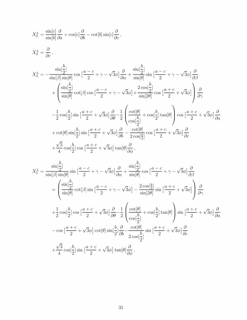
a. The left-invariant vector fields

XL1 =

cos[c]

sin[b]

∂

∂a= sin[c]

∂

∂b− cot[b] cos[c]

∂

∂c,

30

XL2 =

sin[c]

sin[b]

∂

∂a+ cos[c]

∂

∂b− cot[b] sin[c]

∂

∂c,

XL3 =

∂

∂c,

XL4 = −

sin[b

2]

sin[β] sin[θ]cos[a − c

2+ γ −

√3φ] ∂

∂α+

sin[b

2]

sin[θ]sin[a − c

2+ γ −

√3φ] ∂

∂β

+

sin[b

2]

sin[θ]cot[β] cos

[a − c

2+ γ −

√3φ]

+2 cos[

b

2]

sin[2θ]cos[a + c

2+√

3φ]

∂

∂γ

−1

2cos[

b

2] sin

[a + c

2+√

3φ] ∂

∂θ−1

2

cot[θ]

cos[b

2]

+ cos[b

2] tan[θ]

cos[a + c

2+√

3φ] ∂

∂a

+ cot[θ] sin[b

2] sin

[a + c

2+√

3φ] ∂

∂b− cot[θ]

2 cos[ b2]cos[a + c

2+√

3φ] ∂

∂c

+

√3

4cos[

b

2] cos

[a + c

2+√

3φ]

tan[θ]∂

∂φ,

XL5 =

sin[b

2]

sin[β] sin[θ]sin[a − c

2+ γ −

√3φ] ∂

∂α+

sin[b

2]

sin[θ]cos[a − c

2+ γ −

√3φ] ∂

∂β

=

sin[b

2]

sin[θ]cot[β] sin

[a − c

2+ γ −

√3φ]

− 2 cos[ b2]

sin[2θ]sin[a + c

2+√

3φ]

∂

∂γ

+1

2cos[

b

2] cos

[a + c

2+√

3φ] ∂

∂θ−1

2

cot[θ]

cos[b

2]

+ cos[b

2] tan[θ]

sin[a + c

2+√

3φ] ∂

∂a

− cos[a + c

2+√

3φ]

cot[θ] sin[b

2]∂

∂b− cot[θ]

2 cos[b

2]

sin[a + c

2+√

3φ] ∂

∂c

+

√3

4cos[

b

2] sin

[a + c

2+√

3φ]

tan[θ]∂

∂φ,

31

XL6 =

cos[b

2]

sin[β] sin[θ]cos[a + c

2+ γ −

√3φ] ∂

∂α−

cos[b

2]

sin[θ]sin[a + c

2+ γ −

√3φ] ∂

∂β

−

cos[b

2]

sin[θ]cot[β] cos

[a + c

2+ γ −

√3φ]

−2 sin[

b

2]

sin[2θ]cos[a − c

2+√

3φ]

∂

∂γ

−1

2sin[

b

2] sin

[a − c

2+√

3φ] ∂

∂θ−1

2

cot[θ]

sin[b

2]

+ sin[b

2] tan[θ]

cos[a − c

2+√

3φ] ∂

∂a

− cos[b

2] cot[θ] sin

[a − c

2+√

3φ] ∂

∂b+

cot[θ]

2 sin[b

2]

cos[a − c

2+√

3φ] ∂

∂c

+

√3

4cos[a − c

2+√

3φ]

sin[b

2] tan[θ]

∂

∂φ,

XL7 = −

cos[b

2]

sin[β] sin[θ]sin[a + c

2+ γ −

√3φ] ∂

∂α−

cos[b

2]

sin[θ]cos[a + c

2+ γ −

√3φ] ∂

∂β

+

cos[b

2]

sin[θ]cot[β] sin

[a + c

2+ γ −

√3φ]

+2 sin[

b

2]

sin[2θ]sin[a − c

2+√

3φ]

∂

∂γ

+1

2cos[a − c

2+√

3φ]

sin[b

2]∂

∂θ−1

2

cot[θ]

sin[b

2]

+ sin[b

2] tan[θ]

sin[a − c

2+√

3φ] ∂

∂a

+ cos[b

2] cos

[a − c

2+√

3φ]

cot[θ]∂

∂b+

cot[θ]

2 sin[b

2]

sin[a − c

2+√

3φ] ∂

∂c

+

√3

4sin[b] sin

[a − c

2+√

3φ]

tan[θ]∂

∂φ,

XL8 =

1

2

∂

∂φ.

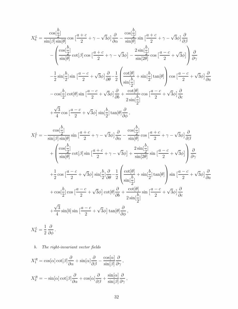
b. The right-invariant vector fields

XR1 = cos[α] cot[β]

∂

∂α+ sin[α]

∂

∂β− cos[α]

sin[β]

∂

∂γ,

XR2 = − sin[α] cot[β]

∂

∂α+ cos[α]

∂

∂β+

sin[α]

sin[β]

∂

∂γ,

32

XR3 =

∂

∂α,

XR4 =

cot[θ]

2 cos[β

2]

cos[α + γ

2]

∂

∂α− cot[θ] sin[

β

2] sin[

α + γ

2]

∂

∂β

+ cos[α + γ

2]

cot[θ]

2 cos[β

2]

− cos[β

2] tan[θ]

∂

∂γ+

1

2cos[

β

2] sin[

α + γ

2]∂

∂θ

−

cot[b]

sin[θ]cos[a − α − γ

2] sin[

β

2] +

cos[β

2]

sin[2θ]cos[

α + γ

2](2 − 3 sin2[θ])

∂

∂a

−sin[

β

2]

sin[θ]sin[a − α − γ

2]∂

∂b+

sin[β

2]

sin[b] sin[θ]cos[a − α − γ

2]∂

∂c

−√

3

4cos[

β

2] cos[

α + γ

2] tan[θ]

∂

∂φ,

XR5 = − cot[θ]

2 cos[β

2]

sin[α + γ

2]

∂

∂α− cos[

α + γ

2] cot[θ] sin[

β

2]

∂

∂β

− sin[α + γ

2]

cot[θ]

2 cos[β

2]

− cos[β

2] tan[θ]

∂

∂γ+

1

2cos[

β

2] cos[

α + γ

2]∂

∂θ

−

cot[b]

sin[θ]sin[a − α − γ

2] sin[

β

2] −

cos[β

2]

sin[2θ]sin[

α + γ

2](2 − 3 sin2[θ])

∂

∂a

+sin[

β

2]

sin[θ]cos[a − α + γ

2]∂

∂b+

sin[β

2]

sin[b] sin[θ]sin[a − α − γ

2]∂

∂c

+

√3

4cos[

β

2] sin[

α + γ

2] tan[θ]

∂

∂φ,

33

XR6 =

cot[θ]

2 sin[β

2]

cos[α − γ

2]

∂

∂α+ cos[

β

2] cot[θ] sin[

α − γ

2]

∂

∂β

− cos[α − γ

2]

cot[θ]

2 sin[β

2]

− sin[β

2] tan[θ]

∂

∂γ+

1

2sin[

β

2] sin[

α − γ

2]∂

∂θ

−

cot[b]

sin[θ]cos[a +

α + γ

2] cos[

β

2] −

sin[β

2]

sin[2θ]cos[

α − γ

2](2 − 3 sin2[θ])

∂

∂a

−cos[

β

2]

sin[θ]sin[a +

α + γ

2]∂

∂b+

cos[β

2]

sin[b] sin[θ]cos[a +

α + γ

2]∂

∂c

+

√3

4cos[

α − γ

2] sin[

β

2] tan[θ]

∂

∂φ,

XR7 =

cot[θ]

2 sin[β

2]

sin[α − γ

2]

∂

∂α− cos[

β

2] cos[

α − γ

2] cot[θ]

∂

∂β

− sin[α − γ

2]

cot[θ]

2 sin[β

2]

− sin[β

2] tan[θ]

∂

∂γ− 1

2cos[

α − γ

2] sin[

β

2]∂

∂θ

−

cot[b]

sin[θ]cos[

β

2] sin[a +

α + γ

2] −

sin[β

2]

sin[2θ]sin[

α − γ

2](2 − 3 sin2[θ])

∂

∂a

+cos[

β

2]

sin[θ]cos[a +

α + γ

2]∂

∂b+

cos[β

2]

sin[b] sin[θ]sin[a +

α + γ

2]∂

∂c

+

√3

4sin[

β

2] sin[

α − γ

2] tan[θ]

∂

∂φ,

XR8 =

√3

∂

∂γ−

√3

∂

∂a+

1

2

∂

∂φ.

34

[1] G. ’t Hooft, “50 Years of Yang-Mills Theory,” World Scientific Publishing, (2005).

[2] C. J. Isham, “Topological and Global Aspects of Quantum Theory,” in Relativity, Groups and

Topology edited by B. DeWitt and R. Stora, North-Holland, 1983.

[3] D. McMullan and I. Tsutsui, “On the Emergence of Gauge Structures and Generalized Spin

When Quantizing on a Coset Space”, Ann. of Phys. 237 (1995) 269.

[4] T. Tilma and E.C.G. Sudarshan, “A Parametrization of Bipartite Systems Based on SU(4)

Euler Angles ”, J. Phys. A: Math. Gen. 35 (2002) 10445-10465

[5] T. Tilma and E.C. Sudarshan, “Generalized Euler Angle Paramterization for SU(N)” , J.

Phys. A: Math. Gen. 35 (2002) 10467-10501

[6] T. Tilma and E.C. Sudarshan, “Generalized Euler Angle Parameterization for U(N) with

Applications to SU(N) Coset Volume Measures”, J. Geom. Phys. 52 (2004) 263-283.

[7] S. Bertini, S.L. Cacciatori, B.L. Cerchiai, “On the Euler Angles for SU(N)”, [arXiv:

math-ph/0510075]

[8] M.S. Byrd, “Differential Geometry on SU(3) with Applications to Three State Systems”, J.

Math. Phys. 39 (1998) pp. 6125-6136. Erratum, J. Math. Phys. 41 (2000) pp. 1026-1030.

[9] M.S. Byrd and E.C. Sudarshan, “SU(3) Revisited”, J. Phys. A 31 (1998) 9255

[arXiv:physics/9803029].

[10] R. Abraham and J.E. Marsden, “Foundations of Mechanics”, Second Edition, Ben-

jamin/Cummings, Reading, Massachusetts, 1978

[11] V.I. Arnold, “Mathematical Methods of Classical Mechanics”, Springer-Verlag, New-York,

1984

[12] S. Kobayashi and K. Nomizu, Foundations of Differential Geometry, I,II, Willey, New York,

1963 and 1969.

[13] S. Helgason, “Differential Geometry, Lie Groups, and Symmetric Spaces”, Academic Press,

Boston, 1978.

[14] According to H. Cheng ang K.C. Gupta, “An Historical Note on Finite Rotations”, Trans.

ASME Journal of Applied Mechanics, 56, 1989, 139-145, the first publication of the derivation

of the Euler angles was posthumous; Leonhard Euler, “De Motu Corporum Circa Punctum

Fixum Mobilium”, Opera Postuma 2, 1862, pp. 43-62. Reprinted in Opera Omnia: Series 2,

35

Volume 9, pp. 413 - 441, Blanc, Charles (Ed.) 1968.

[15] F.D. Murnaghan, “The Unitary and Rotation Groups”, Spartan Books, Washington, 1962

[16] E.P. Wigner, “On a Generalization of Euler’s Angles”, in Group Theory and its Applications,

edited by E.M. Loebl (1968) pp. 119-129.

[17] N. Vilenkin and A. Klimyk, “Representation of the Lie Groups and Special Functions”, Kluwer,

Academic Publishers, Netherlands, 1993

[18] M. Beg and H. Ruegg, “A Set of Harmonic Functions for the Group SU(3)”, J. Math. Phys.

6 (1965) 677.

[19] D.F.Holand, “Finite Transformations and Basis States of SU(n)”, J. Math. Phys. 10 (1969)

1903.

[20] H. Yabu and K. Ando, “A New Approach to the SU(3) Skyrme model”, Nucl. Phys. B 301

(1988) 601.

[21] H. Weigel, “Baryons as Three Flavor Solitons”, Int. J. Mod. Phys. A 11 (1996) 2419.

[22] R. Hermann, “Differential Geometry and the Calculus of Variations”, Academic Press, New

York, 1968.

[23] I.G. Macdonald, “The Volume of a Compact Lie Group”, Invent. Math., 56 (1980) 93-95

[24] C. Bernard, “Gauge Zero Modes, Instanton Determinants, and Quantum Chromodynamics

Calculations”, Phys. Rev. 19 (1979) 3013-3019

[25] L.J. Boya, E.C. Sudarshan and T. Tilma, “Volumes of Compact Manifolds”, Rep. Math. Phys.

52 (2003) 401-422.

[26] L.P. Eisenhart, “Riemannian Geometry”, Princeton University Press, Princeton, 1966.

[27] For a rigorous statement we refer to Theorem 3.2 in [13].

[28] We follow the method of Robert Hermann [22], who attributed this construction to C.C.

Moore.

[29] The freedom of choice in the one-parameter subgroups is analogous to the “x” or “y” Euler

angle representation of SU(2) with freedom to choose either σ1 or σ2.

[30] However, in contrast to the SU(2) group the basic relation defining a space of constant cur-

vature

Rµνσλ =R

n(n − 1)(gµσgνλ − gµλgνσ)

is not valid for the SU(3) group.

36