Sub-THz Component of Large Solar Flares

Emily UlanskiDecember 9, 2008

Plasma Physics and Magnetohydrodynamics

Solar Flares

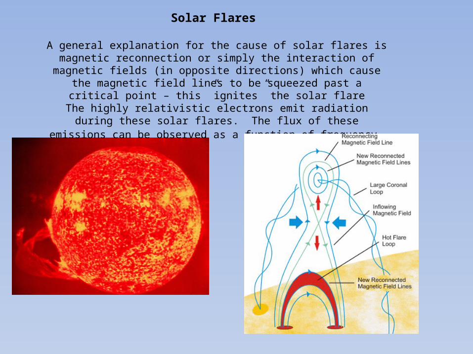
A general explanation for the cause of solar flares is magnetic reconnection or simply the interaction of magnetic fields (in opposite directions) which cause the magnetic field lines to be squeezed past a critical point – this ”ignites” the solar

flareThe highly relativistic electrons emit radiation during these solar flares. The flux

of these emissions can be observed as a function of frequency.

Gyrosynchrotron emission

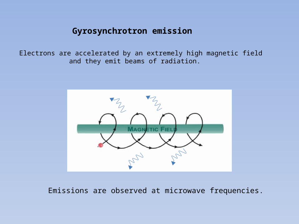
Electrons are accelerated by an extremely high magnetic field and they emit beams of radiation.

Emissions are observed at microwave frequencies.

Frequencies observed during Large Solar flares

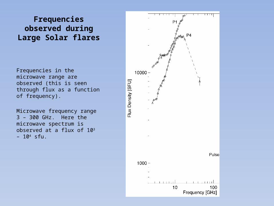
Frequencies in the microwave range are observed (this is seen through flux as a function of frequency).

Microwave frequency range 3 – 300 GHz. Here the microwave spectrum is observed at a flux of 103 – 104 sfu.

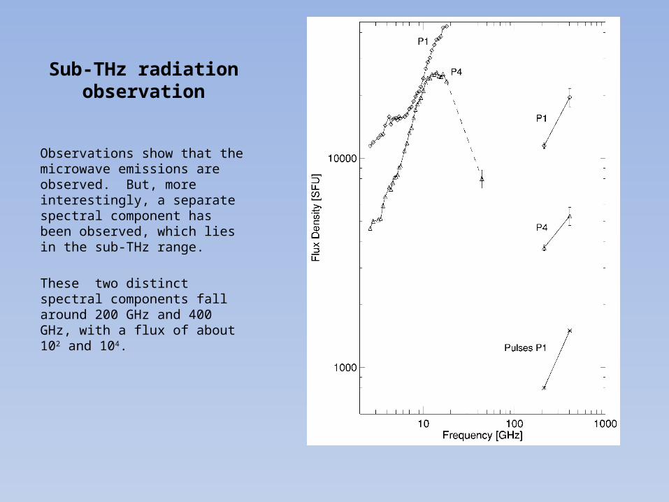
Sub-THz radiation observation

Observations show that the microwave emissions are observed. But, more interestingly, a separate spectral component has been observed, which lies in the sub-THz range.

These two distinct spectral components fall around 200 GHz and 400 GHz, with a flux of about 102 and 104.

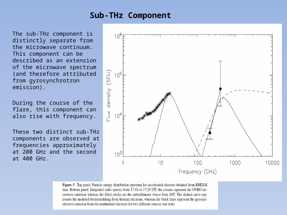
Sub-THz Component

The sub-THz component is distinctly separate from the microwave continuum. This component can be described as an extension of the microwave spectrum (and therefore attributed from gyrosynchrotron emission).

During the course of the flare, this component can also rise with frequency.

These two distinct sub-THz components are observed at frequencies approximately at 200 GHz and the second at 400 GHz.

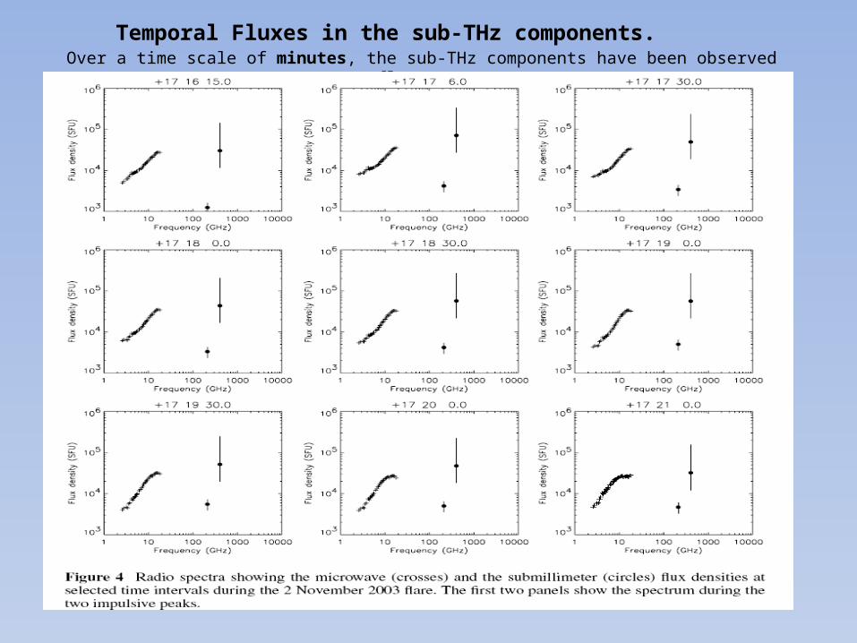
Temporal Fluxes in the sub-THz components.Over a time scale of minutes, the sub-THz components have been observed to fluctuate.

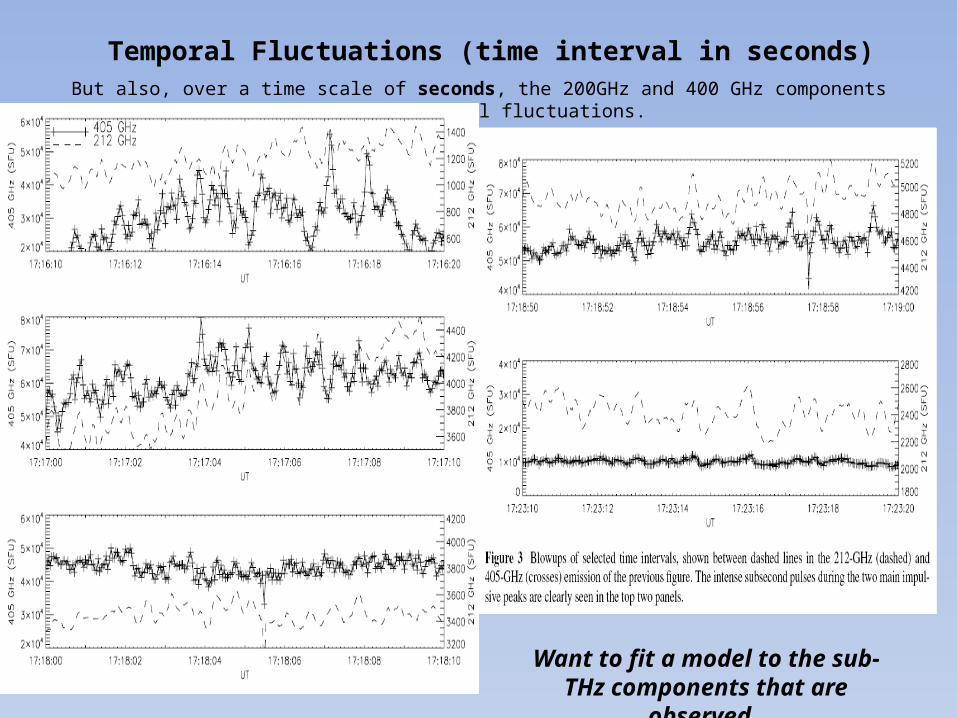
Temporal Fluctuations (time interval in seconds)But also, over a time scale of seconds, the 200GHz and 400 GHz components undergo temporal fluctuations.

Want to fit a model to the sub-THz components that are observed.

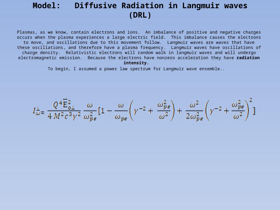
Model: Diffusive Radiation in Langmuir waves (DRL)

Plasmas, as we know, contain electrons and ions. An imbalance of positive and negative charges occurs when the plasma experiences a large electric field. This imbalance causes the electrons to move, and oscillations due to this movement follow. Langmuir waves are waves that have these oscillations, and therefore have a plasma frequency.

Langmuir waves have oscillations of charge density. Relativistic electrons will random walk in langmuir waves and will undergo electromagnetic emission. Because the electrons have nonzero acceleration they have radiation intensity.

To begin, I assumed a power law spectrum for Langmuir wave ensemble..

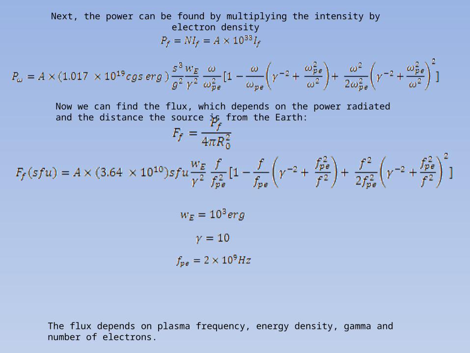
Next, the power can be found by multiplying the intensity by electron density

Now we can find the flux, which depends on the power radiated and the distance the source is from the Earth:

The flux depends on plasma frequency, energy density, gamma and number of electrons.

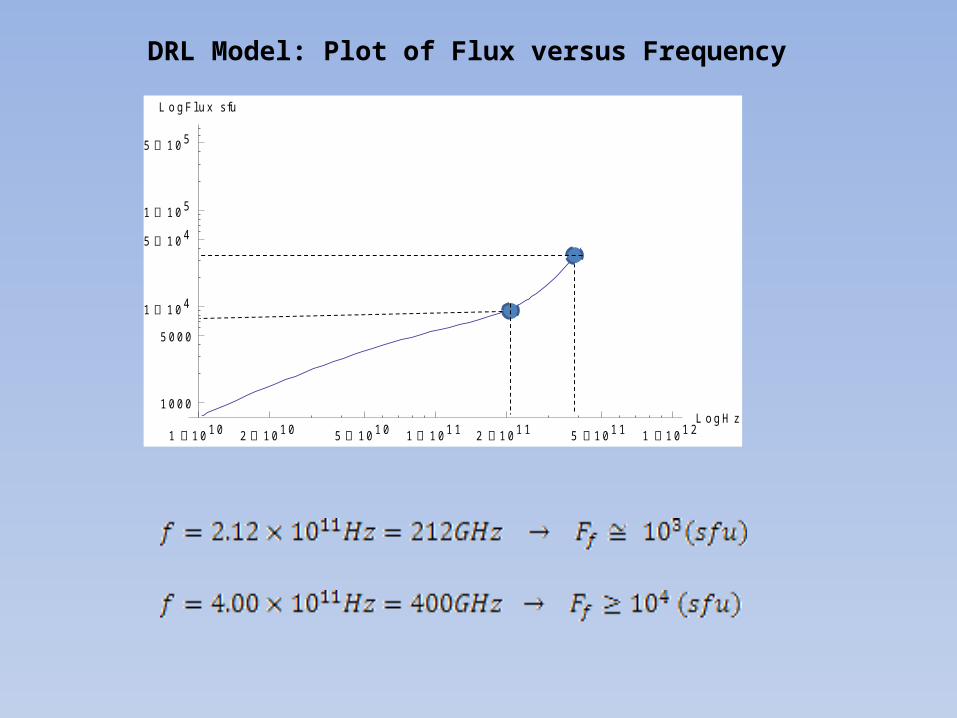
DRL Model: Plot of Flux versus Frequency

1 1010 2 1010 5 1010 1 1011 2 1011 5 1011 1 1012LogHz

1 104

5 1041 105

5 105

1000

5000

LogFlux sfu

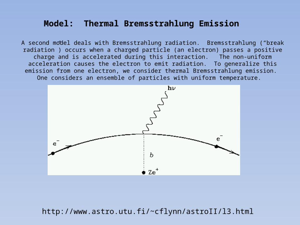
Model: Thermal Bremsstrahlung Emission

A second model deals with Bremsstrahlung radiation. Bremsstrahlung (“break radiation”) occurs when a charged particle (an electron) passes a positive charge and is accelerated during this interaction. The non-uniform

acceleration causes the electron to emit radiation. To generalize this emission from one electron, we consider thermal Bremsstrahlung emission. One considers an ensemble of particles with uniform temperature.

http://www.astro.utu.fi/~cflynn/astroII/l3.html

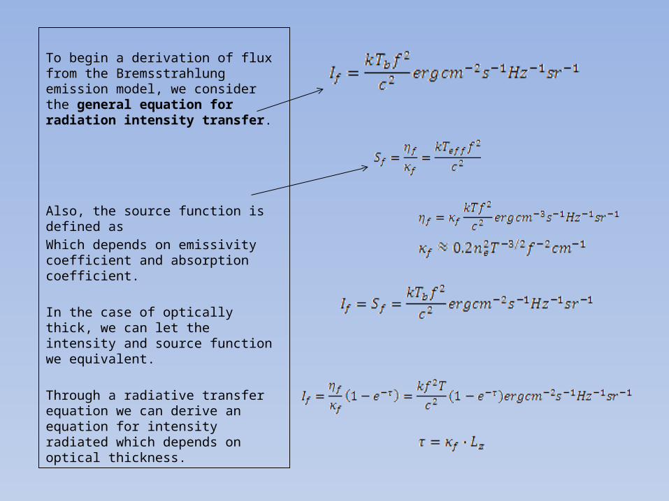
To begin a derivation of flux from the Bremsstrahlung emission model, we consider the general equation for radiation intensity transfer.

Also, the source function is defined as Which depends on emissivity coefficient and absorption coefficient.

In the case of optically thick, we can let the intensity and source function we equivalent.

Through a radiative transfer equation we can derive an equation for intensity radiated which depends on optical thickness.

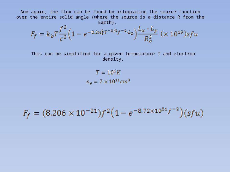
And again, the flux can be found by integrating the source function over the entire solid angle (where the source is a distance R from the Earth).

This can be simplified for a given temperature T and electron density.

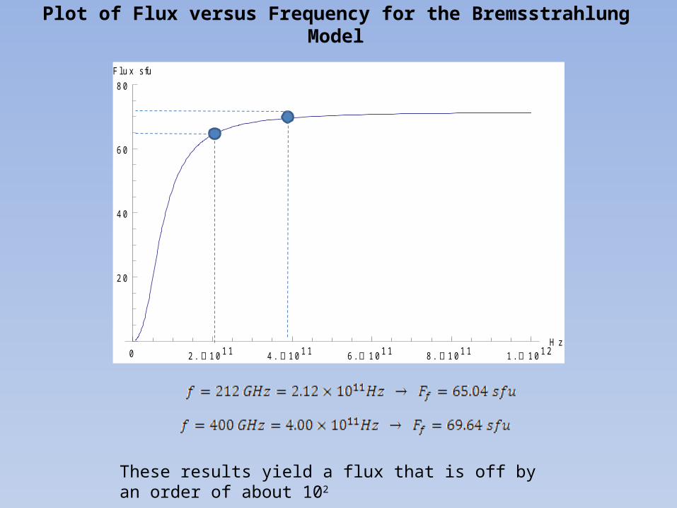
Plot of Flux versus Frequency for the Bremsstrahlung Model

0 2 . 1011 4 . 1011 6 . 1011 8 . 1011 1 . 1012Hz

20

40

60

80Flux sfu

These results yield a flux that is off by an order of about 102

It is also important to look at how changes in electron density change the model

0 2 . 1011 4 . 1011 6 . 1011 8 . 1011 1 . 1012Hz

50

100

150

200

250

300

350Flux sfu

Can see that the electron density does not impact the microwave frequency range.

ne = 4 x 1011 cm3

ne = 3 x 1011 cm3

ne = 2 x 1011 cm3

ne = 1 x 1011 cm3

0 5 . 1010 1 . 1011 1 .5 1011 2 . 1011Hz

20

40

60

80

100Flux sfu Transition from optically thick

to optically thin region

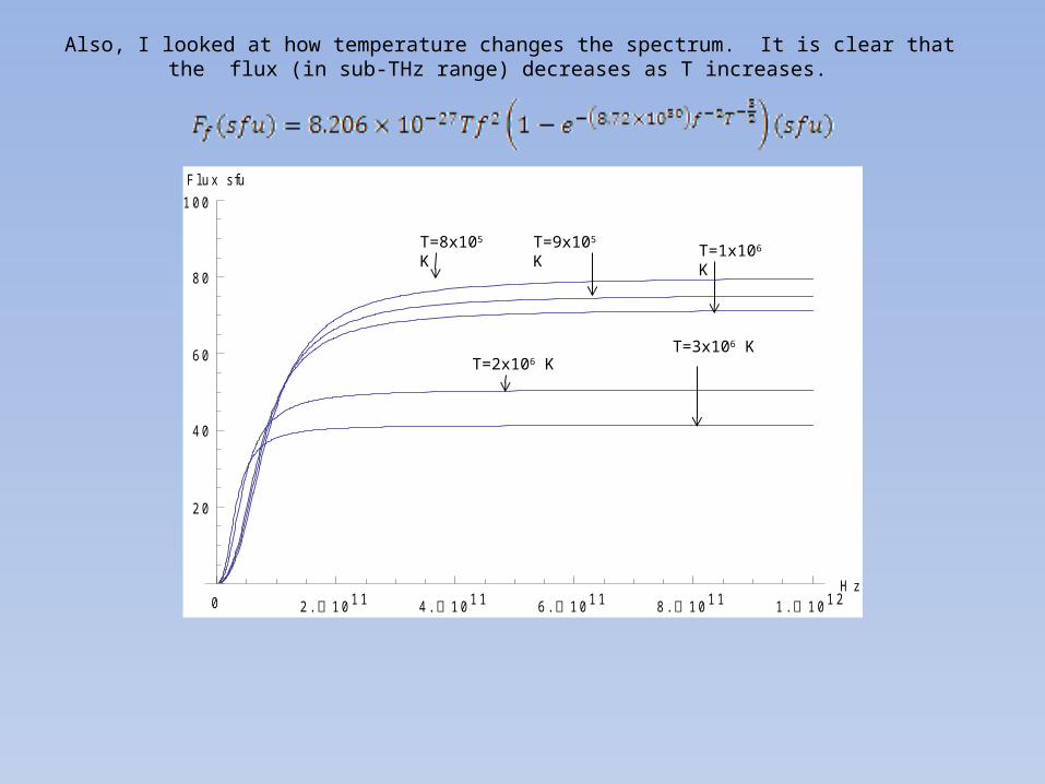
Also, I looked at how temperature changes the spectrum. It is clear that the flux (in sub-THz range) decreases as T increases.

0 2 . 1011 4 . 1011 6 . 1011 8 . 1011 1 . 1012Hz

20

40

60

80

100Flux sfu

T=8x105 K T=9x105 K T=1x106 K

T=2x106 KT=3x106 K

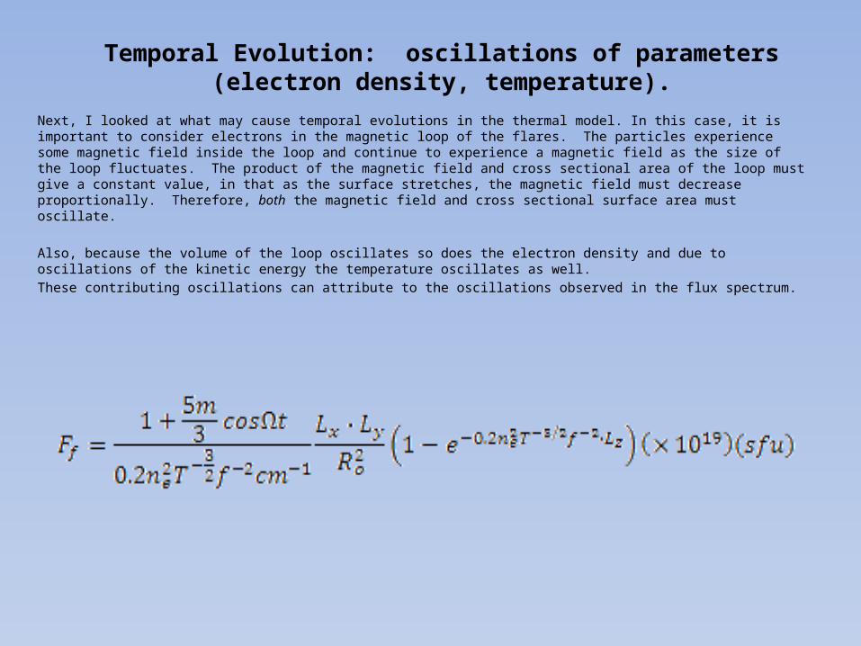
Temporal Evolution: oscillations of parameters (electron density, temperature).

Next, I looked at what may cause temporal evolutions in the thermal model. In this case, it is important to consider electrons in the magnetic loop of the flares. The particles experience some magnetic field inside the loop and continue to experience a magnetic field as the size of the loop fluctuates. The product of the magnetic field and cross sectional area of the loop must give a constant value, in that as the surface stretches, the magnetic field must decrease proportionally. Therefore, both the magnetic field and cross sectional surface area must oscillate.

Also, because the volume of the loop oscillates so does the electron density and due to oscillations of the kinetic energy the temperature oscillates as well. These contributing oscillations can attribute to the oscillations observed in the flux spectrum.

Thank You!