subdivision of texas watersheds for hydrologic modeling

Subdivision of Texas Watersheds for H

ydrologic Modeling

Report No. 0-5822-01-2

Texas Tech University | Lubbock, Texas 79409P 806.742.3503 | F 806.742.4168

Subdivision of Texas Watersheds for Hydrologic Modeling

David B. Thompson and Theodore G. Cleveland

Performed in Cooperation with the Texas Department of Transportation and the Federal Highway Administration

Research Project 0-5822 Research Report 0-5822-01-2 http://www.techmrt.ttu.edu/reports.php

NOTICE

The United States Government and the State of Texas do not endorse products or manufacturers. Trade or manufacturers’ names appear herein solely because they are considered essential to the object of this report

Technical Report Documentation Page

1. Report No.: FHWA/TX -0–5822–01–2

2. Government Accession No.:

3. Recipient’s Catalog No.:

4. Title and Subtitle: Subdivision of Texas watersheds for hydrologic modeling

5. Report Date: June 2009

6. Performing Organization Code: TechMRT

7. Author(s): David B. Thompson, Theodore G. Cleveland

8. Performing Organization Report No. 0–5822–01–2

9. Performing Organization Name and Address: Texas Tech University College of Engineering

10. Work Unit No. (TRAIS):

Box 41023 Lubbock, Texas 79409-1023

11. Contract or Grant No. : Project 0–5822–01–2

12. Sponsoring Agency Name and Address Texas Department of Transportation Research and Technology P. O. Box 5080 Austin, TX 78763-5080

13. Type of Report and Period Cover:

Final project report October 2006 – August 2008

14. Sponsoring Agency Code:

15. Supplementary Notes: This study was conducted in cooperation with the Texas Department of Transportation

16. Abstract: The purpose of this report is to present a set of findings and examples for subdivision of watersheds for hydrologic modeling. Three approaches were used to examine the impact of watershed subdivision on modeled hydrologic response: (1) An equal-area approach, (2) an ad-hoc approach wherein subdivisions were created at locations based on engineering judgment, and (3) a distributed-modeling approach. The three methods were implemented by different individuals with varied hydrologic experience, using their professional judgment under the direction of project researchers. Technology included NRCS curve number method for runoff volume, a variety of runoff-transformation methods, and use of measured rainfall-runoff responses. In general, subdivision had little or no impact on runoff volume. Estimates of peak discharge from study watersheds showed modest improvement in accuracy, but none beyond about 5-7 subdivisions. Time to peak estimates tended to degrade with subdivision, most likely because hydrologic routing introduced additional parameters requiring estimates. The distributed-modeling approach was extremely difficult to apply. In general, subdivision of watersheds is beneficial primarily when flow rates at locations internal to the watershed are required. The improvement in implied accuracy does not generally justify the subdivision process. 17. Key Words Hydrology, watershed, drainage basin, catchment, hydrologic modeling, hydrologic prediction, hydrologic design

18. Distribution Statement No restrictions. Document available to public through TxDOT and TechMRT.

19. Security Classif. (of this report) Unclassified

20. Security Classif. (of this page) Unclassified

21. No. Pages 97

22. Price

Form DOT F 1700.7 (8-72)

This page intentionally left blank.

iii


byDavid B. Thompson, R.O. Anderson Engineering, Inc.

Theodore G. Cleveland, Texas Tech University

with contributions byWilliam H. Asquith, U.S. Geological Survey

Research Report Number 0–5822–2Project Number 0–5822

Project: Subdivision of Watersheds for Modeling

Sponsored by the Texas Department of Transportationin Cooperation with the

U.S. Department of Transportation Federal Highway Administration

Center for Multidisciplinary Research in TransportationDepartment of Civil and Environmental Engineering

Texas Tech UniversityP.O. Box 41023

Lubbock, Texas 79409–1023

June 2009

AUTHOR’S DISCLAIMER

The contents of this report reflect the views of the authors who are responsible for the facts and theaccuracy of the data presented herein. The contents do not necessarily reflect the official view ofpolicies of the Texas Department of Transportation or the Federal Highway Administration. Thisreport does not constitute a standard, specification, or regulation.

PATENT DISCLAIMER

There was no invention or discovery conceived or first actually reduced to practice in the courseof or under this contract, including any art, method, process, machine, manufacture, design orcomposition of matter, or any new useful improvement thereof, or any variety of plant which is ormay be patentable under the patent laws of the United States of America or any foreign country.

ENGINEERING DISCLAIMER

Not intended for construction, bidding, or permit purposes.

TRADE NAMES AND MANUFACTURERS’ NAMES

The United States Government and the State of Texas do not endorse products or manufacturers.Trade or manufacturers’ names appear herein solely because they are considered essential to theobject of this report.

i

This page intentionally left blank.

ii

Acknowledgements

Three graduate students played a large role in the accomplishment of the research reported herein.Ms. Thuy Luong earned her Master of Science degree under the Texas Department of Transporta-tion (TxDOT) Master’s Degree program at University of Houston working on the equal drainage-area problem. Mr. Matthew Wingfield completed his Master of Science degree under the TexasDepartment of Transportation Master’s Degree program at Texas Tech University, working hisway through the ad-hoc approach to watershed subdivision. Ms. Erika Nordstrom wrestled withdistributed modeling under HEC-HMS while earning her Master of Science degree at Texas TechUniversity. Without the efforts of these students, the research reported in this report would nothave been accomplished.

Dr. William Asquith, Ms. Meghan Roussel, and Ms. Sally Holl of the U.S. Geological Survey (USGS)in Austin, Texas provided much-needed help in two major areas. The first was in support of thedistributed modeling problem. It cannot be sufficiently emphasized how difficult it is to createand use fully-distributed models under the current version of HEC-HMS (U.S. Army Corps ofEngineers, 2008). USGS personnel were able to access U.S. Army Corps of Engineers personnel atthe Hydrologic Engineering Center for assistance that would not have been available to universityresearchers. In addition, they provided substantial work on the stochastic approach reported herein.

The support and insight of the TxDOT Project Advisory Committee was invaluable in determiningappropriate research directions. The authors thank the committee for their efforts.

iii

Contents

1 Background 1

1.1 History of the Project . . . . . . . . . . . . . . . . . . . . . . . . . . . . . . . . . . . 1

1.2 Purpose . . . . . . . . . . . . . . . . . . . . . . . . . . . . . . . . . . . . . . . . . . . 2

1.3 Participants . . . . . . . . . . . . . . . . . . . . . . . . . . . . . . . . . . . . . . . . . 2

2 Procedure 3

2.1 Literature Review . . . . . . . . . . . . . . . . . . . . . . . . . . . . . . . . . . . . . 3

2.2 Equal-Area Models . . . . . . . . . . . . . . . . . . . . . . . . . . . . . . . . . . . . . 3

2.3 Lumped Models . . . . . . . . . . . . . . . . . . . . . . . . . . . . . . . . . . . . . . . 8

2.4 Distributed Models . . . . . . . . . . . . . . . . . . . . . . . . . . . . . . . . . . . . . 13

2.4.1 Datasets Used . . . . . . . . . . . . . . . . . . . . . . . . . . . . . . . . . . . 13

2.4.2 Model Development . . . . . . . . . . . . . . . . . . . . . . . . . . . . . . . . 14

2.4.3 Process Submodels . . . . . . . . . . . . . . . . . . . . . . . . . . . . . . . . . 15

2.4.4 Model Operation . . . . . . . . . . . . . . . . . . . . . . . . . . . . . . . . . . 15

2.5 Stochastic Modeling . . . . . . . . . . . . . . . . . . . . . . . . . . . . . . . . . . . . 15

2.5.1 On The Computation of Celerity . . . . . . . . . . . . . . . . . . . . . . . . . 15

2.5.2 The Experimental Approach . . . . . . . . . . . . . . . . . . . . . . . . . . . 16

3 Literature Review 18

4 Results 22

4.1 Equal-Area Models . . . . . . . . . . . . . . . . . . . . . . . . . . . . . . . . . . . . . 22

4.2 Lumped Models . . . . . . . . . . . . . . . . . . . . . . . . . . . . . . . . . . . . . . . 29

iv

4.2.1 Watershed Subdivision . . . . . . . . . . . . . . . . . . . . . . . . . . . . . . . 29

4.2.2 Changes to Parameter Values . . . . . . . . . . . . . . . . . . . . . . . . . . . 33

4.3 Distributed Models . . . . . . . . . . . . . . . . . . . . . . . . . . . . . . . . . . . . . 37

4.4 Stochastic Modeling . . . . . . . . . . . . . . . . . . . . . . . . . . . . . . . . . . . . 41

4.4.1 Example Computation . . . . . . . . . . . . . . . . . . . . . . . . . . . . . . . 45

4.4.2 Caveats . . . . . . . . . . . . . . . . . . . . . . . . . . . . . . . . . . . . . . . 45

5 Summary and Conclusions 47

5.1 Project Findings . . . . . . . . . . . . . . . . . . . . . . . . . . . . . . . . . . . . . . 50

A Equal-Area Modeling Results 56

B Lumped-Parameter Models 57

C Related Documents 71

v

List of Tables

2.1 Watershed characteristics for watersheds studied by Luong (2008). . . . . . . . . . . 5

2.2 Kerby’s roughness parameter (Kerby, 1959). . . . . . . . . . . . . . . . . . . . . . . 7

2.3 Summary of lumped-model watershed characteristics. . . . . . . . . . . . . . . . . . . 10

4.1 Peak discharge analysis from equal-area subdivision approach (Luong, 2008) . . . . . 23

4.2 Time to peak discharge analysis from equal-area subdivision approach (Luong, 2008) 24

4.3 Runoff volume analysis from equal-area subdivision approach (Luong, 2008) . . . . . 24

4.4 Initial and calibrated curve numbers for South Mesquite Creek from the event ofJanuary 1975. . . . . . . . . . . . . . . . . . . . . . . . . . . . . . . . . . . . . . . . 26

4.5 Initial and calibrated timing parameters for South Mesquite Creek from the event ofJanuary 1975. . . . . . . . . . . . . . . . . . . . . . . . . . . . . . . . . . . . . . . . 27

A.1 Curve number for equal-area watersheds and subdivisions from Luong (2008) . . . . 56

B.1 Basin and routing parameters for Walnut Creek, Part 1. . . . . . . . . . . . . . . . 58

B.2 Basin and routing parameters for Walnut Creek, Part 2. . . . . . . . . . . . . . . . 59

B.3 Basin and routing parameters for Ash Creek, Part 1. . . . . . . . . . . . . . . . . . 60

B.4 Basin and routing parameters for Ash Creek, Part 2. . . . . . . . . . . . . . . . . . 61

B.5 Basin and routing parameters for South Mesquite Creek, Part 1. . . . . . . . . . . . 62

B.6 Basin and routing parameters for South Mesquite Creek, Part 2. . . . . . . . . . . . 63

B.7 Basin and routing parameters for Calaveras Creek, Part 1. . . . . . . . . . . . . . . 64

B.8 Basin and routing parameters for Calaveras Creek, Part 2. . . . . . . . . . . . . . . 65

B.9 Basin and routing parameters for Pond-Elm Creek, Part 1. . . . . . . . . . . . . . . 66

B.10 Basin and routing parameters for Pond-Elm Creek, Part 2. . . . . . . . . . . . . . . 67

vi

B.11 Summary of runoff volume analysis. . . . . . . . . . . . . . . . . . . . . . . . . . . . 68

B.12 Summary of peak discharge analysis. . . . . . . . . . . . . . . . . . . . . . . . . . . 69

B.13 Summary of time to peak analysis. . . . . . . . . . . . . . . . . . . . . . . . . . . . 70

vii

List of Figures

2.1 Approximate location of watersheds examined using HEC-HMS in the study. . . . . . . 4

2.2 Subdivision scheme for the Trinity Basin-North Creek. . . . . . . . . . . . . . . . . . 6

2.3 Location of lumped-parameter model study watersheds. . . . . . . . . . . . . . . . . 10

2.4 Watershed subdivision scheme for South Mesquite Creek. . . . . . . . . . . . . . . . 12

4.1 Example observed and model-predicted runoff hydrographs from the equal-area ap-proach. . . . . . . . . . . . . . . . . . . . . . . . . . . . . . . . . . . . . . . . . . . . 25

4.2 Calibration and verification events for South Mesquite Creek from the events ofJanuary 1975 and March 1977. . . . . . . . . . . . . . . . . . . . . . . . . . . . . . . 28

4.3 Runoff volume relative error for Walnut Creek study watershed. . . . . . . . . . . . 29

4.4 Relative error in peak discharge for study watersheds. . . . . . . . . . . . . . . . . . 30

4.5 Relative error in peak discharge for study watersheds. . . . . . . . . . . . . . . . . . 31

4.6 Runoff hydrographs from the event of October 20, 1984 on Walnut Creek. . . . . . . 32

4.7 The impact of extreme parameter changes on the runoff hydrograph from WalnutCreek. . . . . . . . . . . . . . . . . . . . . . . . . . . . . . . . . . . . . . . . . . . . . 34

4.8 The impact of extreme parameter changes on the runoff hydrograph from Ash Creek. 35

4.9 The impact of extreme parameter changes on the runoff hydrograph from SouthMesquite Creek. . . . . . . . . . . . . . . . . . . . . . . . . . . . . . . . . . . . . . . 35

4.10 The impact of extreme parameter changes on the runoff hydrograph from CalaverasCreek. . . . . . . . . . . . . . . . . . . . . . . . . . . . . . . . . . . . . . . . . . . . . 36

4.11 The impact of extreme parameter changes on the runoff hydrograph from Pond-ElmCreek. . . . . . . . . . . . . . . . . . . . . . . . . . . . . . . . . . . . . . . . . . . . . 36

4.12 Relative errors of runoff volume as a function of the number of subdivisions fromdistributed modeling. . . . . . . . . . . . . . . . . . . . . . . . . . . . . . . . . . . . . 38

viii

4.13 Relative errors of peak discharge as a function of the number of subdivisions fromdistributed modeling. . . . . . . . . . . . . . . . . . . . . . . . . . . . . . . . . . . . . 39

4.14 Relative errors in time to peak discharge as a function of the number of subdivisionsfrom distributed modeling. . . . . . . . . . . . . . . . . . . . . . . . . . . . . . . . . . 40

4.15 Observed and modeled runoff hydrograph from Ash Creek for the event of March27, 1977. . . . . . . . . . . . . . . . . . . . . . . . . . . . . . . . . . . . . . . . . . . . 40

4.16 Relation between absolute value of peak streamflow error and celerity factor for twocascading undeveloped sub-watersheds. . . . . . . . . . . . . . . . . . . . . . . . . . . 42

4.17 Relation between absolute value of peak streamflow error and celerity factor for twocascading developed sub-watersheds. . . . . . . . . . . . . . . . . . . . . . . . . . . . 43

ix

1. Background

The purpose of this section of the report is to establish the historical importance of the watershedsubdivision problem and to define project scope and objectives.

1.1. History of the Project

Texas Department of Transportation (TxDOT) engineers are tasked with design of drainage andother hydraulic structures. Such designs require development of estimates of a design discharge. Adesign discharge is the flow rate from the watershed draining to the design point for a given levelof risk, termed either the exceedance probability1 or the return interval2.

One of the technologies used by TxDOT analysts is the hydrograph method. Application of thehydrograph method requires a risk level, estimation of the unit hydrograph, selection of a designhyetograph, and a loss method. Analysts sometimes subdivide the watershed into smaller units foranalysis. It is this subdivision of watersheds that is the topic of this report.

Experienced analysts understand innately that watershed subdivision is sometimes required, butshould be kept to some minimum degree. Why subdivision might be a bad thing is not articulatedclearly either in education of the analyst or in the professional literature. This omission of guidanceleads some analysts to believe that subdivision of a watershed leads to improved estimates3. How-ever, as the number of sub-watersheds increases, so does the number of hydrologic parameters thatmust be estimated. Without substantial supporting data for use in estimating or calibrating theburgeoning parameter set, it is unclear whether anything is gained by the additional work requiredto subdivide the watershed.

Whereas the previous discussion obviously applies to lumped-parameter models, like the hydro-graph method, it also applies to other modeling approaches, including the distributed-modelingapproach and the traditional network rational method. In the former, the watershed is intention-ally discretized into small components, each with a hydrograph-generation model and associatedparameters. The connections between elements can be fairly simple or fairly complex. An example

1The exceedance probability is the probability the given event will be equaled or exceeded over a fixed period oftime, usually one year.

2The terms return interval and recurrence interval are used interchangeably. These terms refer to the average timebetween events of similar magnitude over a relatively long period of time. The long period of time must be severaltimes greater than the return interval. These terms are often misunderstood.

3It is tempting to use the term accuracy, but it is difficult to associate accuracy with hydrologic estimates.

1

of the former is a simple lag time between hydrographs from adjacent elements; an example of thelatter is a hydrodynamic modeling scheme, such as used in the Storm Water Management Model(Rossman, 2008).

The problem with parameter identification and calibration remains, however, whenever a watershedis broken into small components. These issues were a major topic of research interest in the 1980s.Examples are Gupta and Sorooshian (1983), Gupta and Sorooshian (1985b), Gupta and Sorooshian(1985a), Hornberger and others (1985), Jakeman and Hornberger (1993), Loague and Freeze (1985),Sorooshian (1981), Sorooshian and Gupta (1983), and Sorooshian and Gupta (1985). A generalconclusion from these research results is that simplest is best.

As a result of discussions between TxDOT analysts and the research community, a problem state-ment, TxDOT Research Project Number 0–5822 Subdivision of Watersheds for Modeling, wasdeveloped and proposals were solicited. The project began in fiscal year 2007. The objectives ofthe research were:

1. Determine justification and methodology for subdividing watersheds for use with lumpedmodels, and

2. Assess the utility of distributed models, such as the gridded sub-model system of HEC-HMS.

1.2. Purpose

The purpose of this report is to present results of efforts by researchers at Texas Tech University,University of Houston, and U.S. Geological Survey.

1.3. Participants

Besides the principal investigators who were involved in this research, a number of graduate studentscontributed significant efforts. Ms. Thuy Luong worked on the equal watershed area problem. Mr.Matthew Wingfield conducted the lumped-parameter modeling. Ms. Erika Nordstrom fought herway through the distributed modeling problem. The work of these students is contained within thefollowing text.

2

2. Procedure

2.1. Literature Review

A review of the professional literature was undertaken by members of the research team and thegraduate students supporting those researchers. Results of the literature review were not presentedas a separate report, but as a technical memorandum1. A review of the literature is included inthis report as Chapter 3. A map of Texas with the study sites superimposed on it is shown asFigure 2.1.

2.2. Equal-Area Models

Luong (2008) presents one of several approaches to watershed subdivision: the iso-characteristicapproach. In the iso-characteristic approach, watershed subdivision is implemented by creatingsubdivisions such that the characteristic of choice (area, main channel length, etc.) is approximatelyequal for each subdivision.

Luong’s (2008) approach was to first estimate the hydrologic response of a watershed as a singlebasin with no subdivisions. This no-subdivision model formed the basis for comparison of resultsfrom the creation of additional sub-watersheds. The second part of Luong’s (2008) approach was toanalyze the watershed by subdividing it into 2, 3, 5, and 7 sub-basins. These individual sub-basinsresponses are combined to generate a composite response for an entire watershed at the watershedoutlet. The modeled hydrographs are compared with the observed hydrographs to see if the useof watershed subdivisions results in hydrograph reponses equivalent to observations that are moreaccurate than use of a single, un-subdivided watershed. In other words, to determine how thehydrograph response changes as a function of the degree of watershed subdivision.

Five watersheds in Central Texas were selected for study: Onion Creek, South Mesquite, LittleFossil, Olmos Creek, and Trinity Basin-North. Drainage areas for these watersheds ranged fromapproximately 12.3–166 square miles, main channel lengths ranged from approximately 9–48 miles,and dimensionless main channel slopes ranged from approximately 0.002–0.02. Events selected froma database of incremental cumulative rainfall values for storms that occurred during the period1961–1986 (Asquith and others, 2004) were used as input to the HEC-HMS program (U.S. ArmyCorps of Engineers, 2006) to test the iso-characteristic method.

1The technical memorandum documenting the results of the literature review was dated 31 August 2007.

3

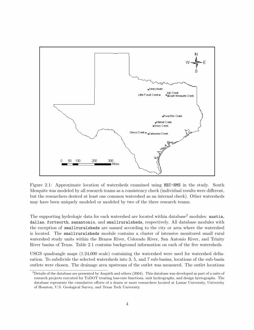
Figure 2.1: Approximate location of watersheds examined using HEC-HMS in the study. SouthMesquite was modeled by all research teams as a consistency check (individual results were different,but the researchers desired at least one common watershed as an internal check). Other watershedsmay have been uniquely modeled or modeled by two of the three research teams.

The supporting hydrologic data for each watershed are located within database2 modules: austin,dallas, fortworth, sanantonio, and smallruralsheds, respectively. All database modules withthe exception of smallruralsheds are named according to the city or area where the watershedis located. The smallruralsheds module contains a cluster of intensive monitored small ruralwatershed study units within the Brazos River, Colorado River, San Antonio River, and TrinityRiver basins of Texas. Table 2.1 contains background information on each of the five watersheds.

USGS quadrangle maps (1:24,000 scale) containing the watershed were used for watershed delin-eation. To subdivide the selected watersheds into 3, 5, and 7 sub-basins, locations of the sub-basinoutlets were chosen. The drainage area upstream of the outlet was measured. The outlet locations

2Details of the database are presented by Asquith and others (2004). This database was developed as part of a suite ofresearch projects executed for TxDOT treating loss-rate functions, unit hydrographs, and design hyetographs. Thedatabase represents the cumulative efforts of a dozen or more researchers located at Lamar University, Universityof Houston, U.S. Geological Survey, and Texas Tech University.

4

Table 2.1: Watershed characteristics for watersheds studied by Luong (2008).

Watershed Module Drainage Main channelarea (mi2) slope

Onion Creek Austin 166 0.026South Mesquite Creek Dallas 23 0.0022Little Fossil Creek Fort Worth 12.3 0.005Olmos Creek San Antonio 21.2 0.0038Trinity Basin/North Creek Smallrural 23.4 0.005

were adjusted until the individual sub-basin areas are about the same.

A discussion of “about the same” is appropriate. The study watersheds were subdivided man-ually using paper maps for watershed delineation and a mechanical planimeter for measurementof drainage area. Equal area subdivision is nontrivial and small movements of the subdivisionoutlet required re-delineation and re-measurement of the drainage area. A particular challengewas the treatment of main-channel tributaries. In many cases inclusion of a tributary channel inone sub-basin resulted in a substantial change to sub-basin drainage area with a small change tothe location of the subdivision point on the main watershed channel. As a result, exact equal-area delineation was practically impossible. This experience alone suggests that prior studies byothers that used stream bifurcation rules encountered similar issues and it is speculated that thesubdivision challenge is in part why these bifurcation schemes exist.

Figure 2.2 is an example of five subdivision configurations for one of the study watersheds, TrinityBasin-North Creek. Once the sub-basin was established, the physical properties of the watershed(and sub-watersheds), such as area, main channel length, and main channel slope were measured.The watershed characteristics were used for estimation of model parameters.

The HEC-HMS models were assembled from the watershed and subdivisions of the watersheds. TheNatural Resources Conservation Service3 (NRCS) curve number procedure was used to representthe rainfall-runoff conversion process. Curve numbers for study watersheds (and their subdivisions)were developed using TR-55 (U.S. Department of Agriculture, Natural Resources ConservationService, 1986) with Hydrologic Soil Group from the Web Soil Survey4 and land-use/land-coverfrom Google Earth5. Impervious area was accounted for using a weighted curve number (McCuenand others, 2002),

CN = CNp(1− f) + 98f, (2.1)

where CNp is the table curve number, f is the fraction of impervious area, and the value 98represents the curve number for impervious areas.

3The NRCS was the Soil Conservation Service (SCS) in a previous incarnation. The acronym, SCS, is retained inthe current version of HEC-HMS (U.S. Army Corps of Engineers, 2006).

4The Web Soil Survey is the database service offered by NRCS through http://websoilsurvey.nrcs.usda.gov atthe time of this writing.

5Google Earth is a freely-available application supported by Google and available from http://earth.google.com/

at the time of this writing.

5

Figure 2.2: Subdivision scheme for the Trinity Basin-North Creek.

6

The NRCS dimensionless unit hydrograph was used as the transform function to compute watersheddischarge from effective precipitation. The time of concentration for each watershed or watershedsubdivision was estimated using a combination of overland flow travel time (Kerby, 1959) andchannel flow time (Kirpich, 1940), based on research conducted under TxDOT project 0–4969(Roussel and others, 2005). Kerby’s (1959) overland flow travel time is

to =[

0.67LNS0.5

], (2.2)

where to is the overland flow travel time (min, time of concentration), L is the length of overlandflow (ft; L should be less than or equal to 600 ft), N is Kerby’s roughness parameter6, and S is theoverland flow slope. Values for Kerby’s retardance coefficient are listed on Table 2.2.

Table 2.2: Kerby’s roughness parameter (Kerby, 1959).

Description N

Pavement 0.02Smooth, bare packed soil 0.10Poor grass, cultivated rowcrops or moderately roughbare surfaces

0.20

Pasture, average grass 0.40Deciduous forest 0.60Dense grass, coniferous forest,or deciduous forest with deeplitter

0.80

Kirpich’s (1940) equation istc = 0.0078L0.77S−0.385, (2.3)

where tc is the channel time of concentration (min), L is the main channel length (ft, the distancefrom the outlet to the distal end of the watershed), and S is the main channel slope (the change inelevation over the main channel divided by the main channel length). The time of concentration forthe watershed is the sum of the overland flow and channel flow portions of the watershed responsetime. The NRCS dimensionless unit hydrograph lag time is

tl = 0.6tw, (2.4)

where tl is the lag time for the watershed (or subdivision) and tw is the watershed (or subdivision)time of concentration.

When the study watershed was subdivided, routing was required to move the subwatershed hy-drograph from the outlet of the subwatershed to the next junction downstream (or the watershed

6Kerby’s N is not Manning’s n, Values for N should be taken from tables of values for Kerby. See Kerby (1959) orHaan and others (1982) for details.

7

outlet). The simple lag routing method was chosen, with the lag time set to the channel time ofconcentration derived from the Kirpich equation. Reach lengths were relatively short so limitedattenuation of routed hydrographs was expected, therefore lag routing was considered appropriate(Dooge, 1973).

The meteorologic model for HEC-HMS was defined using the measured hyetograph for each event mod-eled. In this research, the precipitation was observed rainfall from a historical event. These rainfalldata were taken from a database assembled for previous projects and documented by Asquithand others (2004). Because the rainfall data tabulated with date and time and the accumulatedrainfall were not uniformly spaced (break-point data), the data were converted by interpolation tohave a 5-minute time interval. The arithmetic-mean method was used to determine areal averagerainfall for all sub-watersheds because rainfall observations from only a few gages were availableand the measurements from each gaging station did not differ greatly from the mean, and the pre-cise location of the gages with respect to the watershed were unknown — therefore a complicatedweighting scheme does not make sense7.

Results from the HEC-HMS modeling were measured using three metrics, the mean relative deviation,the root mean square error, and a simple count of the number of times a given subdivision schemeprovided the minimum error. These metrics were applied to peak discharge, Q, time to peakdischarge, tp, and runoff volume, V . The mean relative deviation is

Xd =1N

N∑i=1

(Xs −Xo

Xo

), (2.5)

where Xs is the model value, Xo is the observed value, and N is the number of events. The rootmean square error is

RMSE =

√√√√ 1N

N∑i=1

(Xs −Xo

Xo

)2

. (2.6)

2.3. Lumped Models

Wingfield (2008) used automated tools to conduct watershed delineations and subdivision similarto the approach documented by Luong (2008), but using a different set of watersheds and a dif-ferent subdivision approach. Wingfield’s component of the study also addressed slightly differentquestions:

1. What fraction of a watershed must be different to justify a subdivision?

2. Where must the analyst expend effort to produce good estimates?

Wingfield’s objectives were:7Actual gage locations appear on watershed maps in the original sources used to construct the database.

8

1. To use ArcGIS and the extension tools ArcHydro (Maidment, 2002) and HEC-GeoHMS (U.S. ArmyCorps of Engineers, 2003) to delineate watersheds and sub-watersheds and to extract modelingparameters for each,

2. To evaluate the enhanced or diminished prediction value on watershed modeling as a functionof subdivision, and

3. To determine if there is a certain percentage of a watershed that needs to be significantlydifferent from the rest in order to justify subdividing.

The approach used to accomplish the objectives of this component of the project was:

1. Use the extension tools ArcHydro (Maidment, 2002) and HEC-GeoHMS (U.S. Army Corps ofEngineers, 2003) within ArcGIS, to delineate the study watersheds and to extract modelparameters for each watershed (drainage areas, curve numbers, channel slopes, etc.),

2. Use HEC-HMS (U.S. Army Corps of Engineers, 2008) to compute runoff hydrographs for thevarious subdivision schemes, and

3. Use the lumped and subdivided watershed models from the previous step and modify sub-stantially one of three watershed parameters (curve number, basin transformation time, orrouting time) for approximately 1/5, 1/3 and 1/2 of the total watershed area to assess sen-sitivity of model output to changes in model parameters. These modifications, in order, areanticipated to impact the runoff generation component (overall mass balance), time redistri-bution of rainfall excess at either the watershed outlet or routing inlet (peak discharge, peakarrival, and sub-basin hydrograph shape), and time redistribution of recombined hydrographswhen routing is present in the model (peak discharge, peak arrival, and outlet hydrographshape).

Five watersheds were selected for this research project: Walnut Creek, Ash Creek, South MesquiteCreek, Calaveras Creek, and Pond-Elm Creek. Watershed drainage areas ranged between 7.1–46.1 square miles. The watersheds were selected based on certain attributes unique to each one.The locations of the watersheds are shown on Figure 2.3.

Walnut Creek is located near Austin and is considered an urban watershed. The watershed ismostly developed, but does have areas that are undeveloped. Ash Creek and South MesquiteCreek are both located in Dallas and are urban watersheds. Ash Creek contains two distinctsections within the watershed. The northern 1/3 of the watershed is relatively flat and does nothave distinct channel segments, while the southern 2/3 contains steeper sections and has distinctchannel properties. South Mesquite Creek has a main channel running almost the entire lengthof the watershed with relatively short side branches. South Mesquite Creek is also a commonwatershed between completed and concurrent research projects.

Calaveras Creek is located in a rural part of Texas near San Antonio and is mostly undeveloped.It has a distinct main channel section with multiple branching side channels. Pond-Elm Creek is

9

Figure 2.3: Location of lumped-parameter model study watersheds.

also an undeveloped watershed located in a rural section of Texas. This watershed contains a longslender channel along the western side of the watershed and has relatively flat areas at the upstreamend. These five watersheds are summarized in Table 2.3 below. Maps showing each watershed arepresented in Appendix B.

Table 2.3: Summary of lumped-model watershed characteristics.

Watershed USGS North West Development Areastation latitude longitude class mi2

Walnut Creek 08158200 30◦22’30” 97◦39’37” Urban 26.5Ash Creek 08057320 32◦48’18” 96◦43’04” Urban 7.7South Mesquite Creek 08061950 32◦04’32” 96◦34’12” Urban 23.3Calaveras Creek 08182400 29◦22’49” 98◦17’33” Rural 7.1Pond-Elm Creek 08108200 30◦55’52” 97◦01’13” Rural 46.1

For this research, a heuristic approach was chosen based on analyst expertise and judgment. A

10

consequence is that a subdivision scheme applied to one watershed may not apply to anotherwatershed. The criteria used for the location of the watershed subdivisions are:

1. Subdivide where there is a distinct change in land use or land cover,

2. Subdivide where there is a noticeable change in channel or watershed slope, and

3. Subdivide in areas where there are stream branches within the drainage network.

For example, if a mostly-urban watershed had a section that was undeveloped according to theNational Land Cover Database (NLCD), then this undeveloped area would be separated from thetotal watershed. Next, areas which could no longer be subdivided according to differences in landuse or land cover characteristics were subdivided based on changes in the watershed slope. Asthe number of subdivisions increased and the sub-watershed areas decreased, land use and slopesbecame relatively consistent across each sub-watershed. When this happened, stream brancheswithin the drainage network determined subdivision locations.

Each of the five study watersheds was subdivided into 3, 5, 7, 10, 15, and 30 sub-watersheds usingthe method described above. The sub-watershed configurations for South Mesquite Creek areshown in Figure 2.4. Maps showing the location of the subdivisions for the remaining watershedsare presented in Appendix B.

Three metrics were used to evaluate differences between computed and observed runoff hydrographs.These metrics used the concept of relative error, as expressed in Equation 2.7,

Re =(|Xc −Xo|

Xo

), (2.7)

where Re is the relative error (dimensionless), Xc is the computed value, and Xo is the observedvalue. For each storm event and subdivision scheme, the relative error was computed for runoffvolume, peak flow, and time to peak. In a “perfect” hydrologic model, the relative error is zerofor all events. Two versions of the relative error were used to assess model results directly, and theimpact of subdivision on computed values. The first is the arithmetic mean of the relative error,

Re =1N

∑Re, (2.8)

where N is the number of observations. The second is the root mean square error,

RMSE =

√1N

∑(Re)

2. (2.9)

The third measure of error was the count of the number of storms for which a particular subdivisionscheme presented the least error in comparison to the others.

11

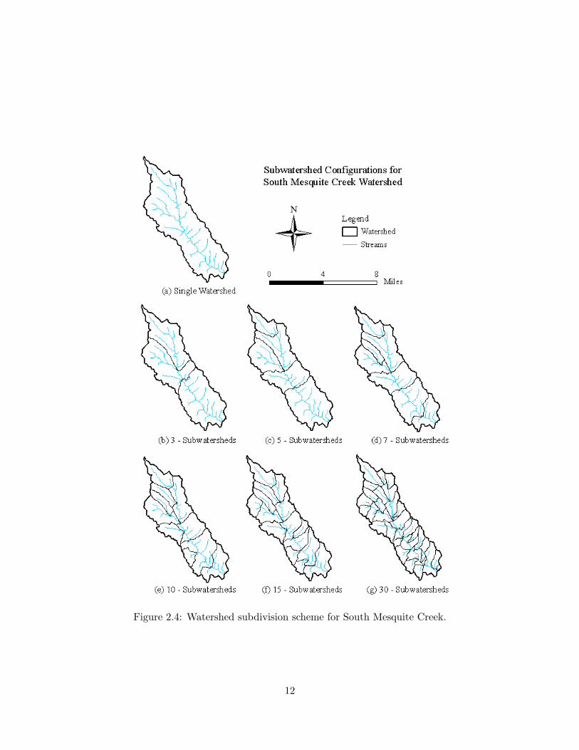
Figure 2.4: Watershed subdivision scheme for South Mesquite Creek.

12

2.4. Distributed Models

Application of distributed models8 was examined using the U.S. Army Corps of Engineers (USACE)HEC-HMS (U.S. Army Corps of Engineers, 2008) model. Although most applications of HEC-HMS arein lumped-parameter mode, the USACE included a gridded hydrologic model in recent versions ofthe program. The Geographic Information Systems (GIS) tools, ArcHydro (Maidment, 2002) andGeoHMS (U.S. Army Corps of Engineers, 2003) were used as preprocessors to generate the distributedHEC-HMS models. Although the GeoHMS program used was the current version (for ArcGIS version9.x, GeoHMS version z041708), the documentation was for Version 1.1 (supported under ArgGIS 3.x)and is several generations behind the distributed version of the program. At least, the softwareand the documentation were not compatible. This was an issue in development of the distributedmodels and is explained in Section 4.3.

Three watersheds were included in the study dataset: Ash Creek, Little Pond-Elm Creek, andSouth Mesquite Creek. Locations of these watersheds are displayed on Figure 2.3. A summary ofstudy watershed characteristics is listed in Table 2.3.

The objectives of this component of the research project were to: (1) Assess the utility of distributedmodeling in an uncalibrated mode that approximates the approach used in engineering practice and(2) Measure differences attributable to increased levels of watershed subdivision in an uncalibratedmode. The three study watersheds were subdivided into 1, 2, 3, 5, 7, and 9 sub-watersheds. Resultsfrom each group were extracted for comparison.

2.4.1. Datasets Used

Use of the distributed model represented by HEC-HMS requires a substantial amount of data anddata processing. This is true of any distributed model. Furthermore, the more detailed the model,the greater the amount of data required. Freely-available datasets were used to develop the models.Spatial datasets used were:

Topography: Topographic data were extracted from the USGS seamless topographic NationalElevation Dataset (NED) 30 m digital elevation model9;

Land Cover: 2001 land cover was obtained from USGS NED (separate data layer);

Soils: the Soil Survey Geographic (SSURGO) database10 was used for soil data; and

Hydrography: The National Hydrographic Database11 was used to define stream locations.8In this research, manual and automated tools were used to construct lumped and subdivided watersheds. Thesubdivided watersheds are in some sense distributed models, however in this project the term fully-distributedrefers to models where gridded data were used to generate hydrographs (and routing) using automated tools withlittle operator intervention.

9The NED web site was http://seamless.usgs.gov/ as of this writing.10The SSURGO web site was http://soils.usda.gov/survey/geography/ssurgo/ at the time of this writing.11The NHD web site was http://nhdgeo.usgs.gov/viewer.htm at the time of this writing.

13

The project coordinate system was Universal Transverse Mercator (UTM) Zone 14N, NationalDatum of 1983. USGS rainfall-runoff data were taken from the dataset documented by Asquithand others (2004). Curve numbers were taken from TR-55 (U.S. Department of Agriculture, NaturalResources Conservation Service, 1986) and from Viessman and Lewis (2003).

2.4.2. Model Development

Development of distributed models using HEC-HMS requires a substantial amount of dataset prepro-cessing. The process involves integration of a variety of datasets from multiple sources and is nottrivial. The steps required are:

1. Terrain preprocessing,

2. Watershed processing,

3. Curve-number generation,

4. HEC-HMS project setup,

5. Basin processing,

6. Basin characteristic development,

7. Hydrologic parameter development,

8. HEC-HMS file creation, and

9. Application of HEC-HMS.

Each of these high-level operations comprises a number (sometimes substantial) of sub-tasks. Fur-thermore, although the basic data were reused for each subdivision iteration, a significant numberof the steps were repeated for each iteration.

Once the watershed grid was established, it was not changed. That is, a 30-meter grid was estab-lished when using the digital elevation model. This grid served as the basis for model developmentthroughout the subdivision process. USGS personnel used the grid system established for water-shed processing to produce a gridded precipitation dataset12 for the hydrologic modeling. Theprecipitation dataset was developed using USACE tools that are generally unavailable to engineersoutside the federal government (unreleased tools). The Asquith and others (2004) dataset providedthe point measurements of rainfall used for the distributed modeling.12The grids were created for 100-meter grid cells. The original DEM was a 30-meter DEM. However, there are

processes to “convert” or create different sized grids. The 100-meter grid-cell size was used for compatibility withgridded precipitation data, which were created using 100-meter grid cells. The GIS-created grid was adjusted to“match” the precipitation grid.

14

2.4.3. Process Submodels

HEC-HMS requires three components for operation: a basin model, a meteorologic model, and acontrol specification. The bulk of the work presented in Section 2.4.2 is preparatory to buildingthe basin model (or sub-basin models). The process sub-models chosen for this analysis are thegridded version (U.S. Army Corps of Engineers, 2000) of the Natural Resources Conservation Service(NRCS) curve number method (U.S. Department of Agriculture, Natural Resources ConservationService, 1997). Flow is routed across each sub-basin using the modified-Clark13 (U.S. Army Corps ofEngineers, 2008). For the time of concentration, the Kirpich (1940) equation was used to representtravel time in channelized portions of the watershed14.

2.4.4. Model Operation

After assembling the required datasets using HEC-GeoHMS and the watershed models using HEC-HMS,HEC-HMS was operated for each event in the study dataset and each subdivision scheme. Resultswere extracted from HEC-HMS and analyzed. The distributed-modeling results are presented inSection 4.3.

2.5. Stochastic Modeling

One of the approaches for modeling a watershed is the application of a set of single-purpose, custom-built programs developed by USGS personnel as part of the suite of research projects of which theproject reported herein is one. These programs are in the R statistical system (R DevelopmentCore Team, 2006) and are based on the technology developed by USGS researchers and publishedin Asquith and Thompson (2003), Roussel and others (2005), and Asquith and Roussel (2007).

2.5.1. On The Computation of Celerity

Where a watershed is subdivided, the celerity Vck in units of length per time is needed to parame-terize a part of a hydraulic routing procedure. This requirement cannot be avoided — one or moreestimates of Vck are needed. It is well known that Vck is a function of many hydraulic parameters,such as channel roughness; channel width, depth, localized slope; and other factors. These valuesare not well constrained for an arbitrary watershed when a hydrologic model of the rainfall-runoffprocess is to be used. Worse, as in the case of slope, the other hydraulic parameters often are highlylocalized — they can vary substantially at the reach scale.13Sometimes referred to (in the USACE documentation, for instance) as the “modClark” algorithm.14All distributed models were developed using only the Kirpich (1940) method. A second set of models were developed

using Kirpich (1940) plus 30 minutes (to account for overland flow travel time). The 30-minute overland flow traveltime was added to the time of concentration for each sub-basin in all models. Only the models using Kirpich (1940)are reported herein.

15

Further, direct computation of storm-to-storm or watershed-to-watershed Vck in the context ofanalysis of the rainfall-runoff process is extremely problematic because the rainfall and runoffresponses of whole watersheds typically are studied.15 As an example, U.S. Geological surveystreamflow-gaging stations are generally operated in comparatively isolated watersheds for thosewatersheds having drainage areas less than about 50 square miles. Hence the recorded streamflowdata fundamentally represent the aggregation of subwatershed response and internal routing.

A special study of a value, ck, that philosophically takes the place of Vck was made as part ofthis research project. Hereafter, this value is referred to as a celerity ck, but acknowledgment(no emphasis) is made that ck does not result from hydraulic analysis, but results from hydrologicanalysis.16 An experimental approach is reported here that explores the nature of ck using stochasticsimulation of 3 inches of uniformly distributed rainfall over 1 hour in twelve 5-minute increments.This rainfall was uniformly distributed over a hypothetical 24 square mile watershed (Ao = 24).This hypothetical watershed is not rocky [R = 0 in the parlance of Asquith and Roussel (2007)],has a main-channel length of 6 miles (Lo = 6), has dimensionless main-channel slope S of 0.004,and curve number CN of 86.

2.5.2. The Experimental Approach

A primary assumption made for the experimental approach reported here is that the proceduresof Asquith and Roussel (2007) represent state-of-the-practice. These procedures represent a fullylumped statistical method for computation of peak streamflow Qp and time of peak streamflow TQp

for arbitrary watersheds. Specifically, the procedures produce the optimal value for Q(AR)p given

the watershed characteristics and input storm hyetograph. In summary, the Asquith and Roussel(2007) procedures outline methods to estimate the loss-rate parameters initial abstraction IA ininches, constant loss CL in inches per hour of a watershed-loss model and to estimate the unithydrograph parameters Tp in hours, and qp in inches per hour of a gamma unit hydrograph. Thesefour values can be stochastically simulated by independent simulation using the t-distribution andthe equations for prediction intervals outlined by Asquith and Roussel.

Given that Q(AR)p can be simulated, in a watershed subdivision context, it follows to seek values for

ck that optimize the estimation of Qp from routing of streamflow (Q(route)p ). The optimization was

made by minimization of ε(ck) = |Q(route)p − Q(AR)

p |, which is the absolute value of the differencebetween discharge estimates. A stochastic approach was used, therefore the streamflow values werereplaced by expectations or

ε(ck) = |E[Qi(route)p ]− E[Qi(AR)

p ]| (2.10)

where E[ ] is the expectation operator, i represents the ith simulation run, and Qi(AR)p represents

individual realizations of the Asquith and Roussel procedures.

The values Qi(route)p in Equation 2.10 are for a subdivided watershed and hence involve simultaneous

15Watersheds are remarkable signal integrators.16It should be remarked however, that channel hydraulics in a regional context are silently represented in the

hydrologic data available to the research team.

16

application of Asquith and Roussel procedures and a method of streamflow routing. The Musk-ingum method was used for routing downstream a distance H, and the method requires an estimateof celerity ck and an X coefficient. The coefficient X is constrained on the interval [0, 0.5] and typ-ically has a value of about 0.2 in natural channels. Lacking of any other source of information forthe purposes of the experimental approach, a triangular distribution of X (X | 0 ≤ X ≤ 0.5) withthe mode at 0.25 was used.

At this point values for ck are the only remaining component for full-out simulation of watershed re-sponse to the input rainfall given watershed (and sub-watershed) characteristics, inter-connections(represented by an addressing and reach-length scheme) between sub-watersheds, and the Musk-ingum routing parameter X.

As a first-order approximation of flow velocity, the ratio of a length to a characteristic time wasused. The selected values of length and time were (1) the main-channel length L and (2) time ofconcentration Tc. Asquith and Roussel (2007) used a time to peak Tp, but Tc seems more intuitivelyuseful than Tp for velocity computations. (The length L is not the length for which the streamflowwill be routed.) Using the conclusions of Roussel and others (2005, p. 15) concerning the relationbetween Tp and Tc the following approximation for ck in feet per second was made

ck ≈

{η(D=0)L[feet]/T

[seconds]c = η(D=0)L[feet]/(T [seconds]

p /0.7) for D = 0η(D=1)L[feet]/T

[seconds]c = η(D=1)L[feet]/(T [seconds]

p /0.4) for D = 1.(2.11)

where the units are shown for specificity and η(D=0|1) represents a celerity factor or magic coefficientthat can be selected in such a fashion as to minimize Equation 2.10.

17

3. Literature Review

The purpose of this literature review is to examine some of the professional literature to deter-mine what other researchers attempted and the results of their work in the context of watershedsubdivision. Additional documents reviewed but not described in this chapter are discussed inAppendix C.

Hromadka II (1986) developed an application manual for hydrologic design for San BernardinoCounty. In that manual, mechanics were developed based on the Los Angeles hydrograph method.In application of the methods presented in the manual, Hromadka II and DeVries: Arbitrary sub-division of the watershed into subareas should generally be avoided. It must be remembered that anincrease in watershed subdivision does not necessarily increase the modelling [sic] “accuracy” butrather transfers the model’s reliability from the calibrated unit hydrograph and lag relationships [sic]to the unknown reliability of the several flow routing submodels used to link together the severalsubareas.

Wood and others (1988) examined the relation between watershed scale and watershed runoff onthe 6.5 mi2 Coweeta River experimental watershed located in North Carolina. Wood and othersdivided the Coweeta River watershed into 3, 19, 39, and 87 sub-watersheds. TOPMODEL (Beven andKirkby, 1979) was used as the simulation engine, with watershed topography from a 30-meter digitalelevation model, and other model parameters and variables randomly sampled from distributions.TOPMODEL was operated using five samples and results aggregated.

Wood and others reported that below a drainage area of about 0.4 mi2, subwatershed responsewas highly variable. However, at scales greater than about 0.4 mi2, further aggregation of sub-watersheds had little impact of simulated results. Therefore, for the Coweeta River watershed, ascale of about 0.4 mi2 seemed appropriate. It is important to observe, however, that the interestof Wood and others (1988) was in determining what they termed the representative elemental areafor the Coweeta River watershed (if such a concept exists) and not in determining the impact ofwatershed subdivision on runoff hydrographs directly. Therefore, whereas the Wood and others(1988) study is interesting (and the sole application of TOPMODEL to this problem), the study doesnot directly apply to the current research problem1.

Sasowsky and Gardner (1991) applied the SPUR model to a 56 mi2 subwatershed of the WalnutGulch experimental watershed in Arizona. The SPUR model operates on a daily time step and wasdesigned for rangeland watersheds. A GIS procedure was used for watershed subdivision based onstream order, an approach not used by other researchers. The result was that the study watershed

1As an aside, no definition of representative elemental area was discovered.

18

was broken into 3, 37, and 66 contributing sub-watersheds. The model was then calibrated againstmeasured rainfall-runoff sequences. The calibration of model parameters is another approach notcommon among the other papers reviewed for the TxDOT project.

Sasowsky and Gardner used the “efficiency” statistic (Nash and Sutcliffe, 1970) to asses modelperformance on a monthly basis, that is, monthly runoff volumes were used to measure modelaccuracy. An efficiency greater than one represents a model that performs better than using themean runoff only. Sasowsky and Gardner (1991) reported that simulations were sensitive to thedegree of watershed subdivision, with lower values of curve number for greater subdivision. This isconsistent with the report of Norris and Haan (1993), who observed that increasing the degree ofsubdivision increased peak runoff for storm-event simulation. The Norris and Haan did not calibratemodel parameters to adjust model-output to match observations; they used a synthetic approach.Sasowsky and Gardner calibrated each “model” (instance of subdivision) to measured rainfall-runoff events, and then noticed that the curve number, in particular, decreased with increasingsubdivision. Although differing in approach to the problem, the results (either increasing dischargein the case of Norris and Haan or decreasing curve number in the case of Sasowsky and Gardner)reported by Sasowsky and Gardner are similar to the those reported by Norris and Haan.

Norris and Haan (1993) used a synthetic method to study the impact of watershed subdivision onhydrographs estimated using the Natural Resources Conservation Service (NRCS, then SCS) unithydrograph procedure, as implemented in HEC-1. The Little Washita watershed near Chickasha,Oklahoma, which has a drainage area of about 59 mi2, was used as the study watershed. Thewatershed was subdivided into 2, 5, 10, and 15 sub-watersheds, as well as treating the watershedas a whole. A balanced hyetograph was used to drive hydrograph computations, with a durationof 24 hours and a return period of 50 years. Results from Norris and Haan (1993) were thatwatershed subdivision had a pronounced impact on the estimate of peak flow from the watershed.The change from a single watershed to 5 sub-basins resulted in a net increase in peak discharge ofabout 30 percent. Use of 15 sub-basins increased the difference from a single watershed to about40 percent. However, the impact of increased subdivision diminished with increasing sub-basincount.

Based on their synthetic study (no observed hydrographs were used to assess model performance),Norris and Haan concluded that the number of sub-basins for simulating watershed response shouldnot vary through the course of a hydrologic study. If the watershed discretization scheme is changedduring a hydrologic study, then the impact of changes in land-use (or other changes) may easily bemasked by differences arising from the subdivision scheme. It was not clear from the report whetherany assessment was made concerning which level of subdivision, if any, was most appropriate forreproduction of watershed hydrographs.

Michaud and Sorooshian (1994) applied three different model formulations to Walnut Creek Gulchin Arizona: KINEROS-complex, KINEROS-simple, and the curve-number approaches were used tosimulate the rainfall-runoff process. The authors reported that KINEROS (in either form) was notable to produce reasonable solutions comparable to observations. In addition, results from appli-cation of the curve number-approach did not compare well with observations.

As a note to the Michaud and Sorooshian report, Loague and Freeze (1985) report an attempt

19

to apply three very different modeling approaches to a set of watersheds. Loague and Freeze alsoreport mixed results from their modeling. In fact, their recommendation is that simpler modelsappear to perform better than more complex approaches.

Mamillapalli and others (1996) conducted a study of the impact of watershed scale on hydrologicoutput. As with many of the studies reported in the journal literature, the NRCS Soil and WaterAnalysis Tool (SWAT) model was used, with a Geographic Information Systems procedure usedto develop the required input streams. Mamillapalli and others conclude: The results indicatethat in general, increasing level of discretization and increase in the number of soil and landusecombinations increases the level of accuracy. There is a level beyond which the accuracy cannot beimproved, suggesting that more detailed simulation may not always lead to better results.

Bingner and others (1997) applied the SWAT to the Goodwin Creek watershed in northern Missis-sippi. SWAT uses the uniform soil-loss equation and its variants to predict sediment yield from thestudy watershed. Their objective was to determine the degree of watershed subdivision required toachieve reasonable results in predicting watershed runoff and sediment yield. Watershed drainagearea of the Goodwin Creek Watershed was about 8.2 mi2. A suite of subdivisions was generatedwith elemental areas that ranged from a maximum of 60 acres to a minimum of 4 acres was used tomodel runoff and sediment yield. The authors concluded that model-predicted runoff volume wasnot heavily dependent on the degree of watershed subdivision but that model-predicted sedimentyield did depend on the degree of watershed subdivision.

FitzHugh and Mackay (2000) conducted a study similar to Bingner and others (1997) for thePheasant Branch watershed in Dane County, Wisconsin. FitzHugh and Mackay also report thatmodel-predicted watershed runoff is not heavily dependent on the degree of subdivision (also usingthe SWAT model), but that model-predicted sediment yield does depend on the degree of subdivision.

Hernandez and others (2002) present results from development of the Automated Geospatial Wa-tershed Assessment (AGWA) tool. The purpose of the software tool is the development of inputparameter sets for the KINEROS and SWAT watershed models. The authors did not specifically testthe impact of watershed subdivision on model performance. However, the authors reported thatresults from application of the SWAT model differed substantially from observations for the twowatersheds tested.

Jha (2002) and Jha and others (2004) examined the relation between watershed subdivision andwater-quality model results. He applied the SWAT model to four Iowa watersheds. Jha and Jhaand others reported that streamflow is not significantly affected by a decrease in sub-watershed scale,with model-predicted results stabilizing with about ten subdivisions. However, model-predictedsediment yields were more dependent on subwatershed scale, requiring 40–50 divisions to stabilizemodel-predicted sediment yield.

Tripathi and others (2006) applied the SWAT model to the 35 mi2 Nagwan watershed in easternIndia. The watershed was subdivided into 12 and 22 sub-watersheds, as well as treating the entirewatershed as a whole. Four years of record were used to operate the model. The model wascalibrated to produce best estimates of model parameters.

20

Tripathi and others report little difference in watershed runoff in response to the number of sub-watersheds. However, they observed variations in other components of the hydrologic cycle. Esti-mates of evapotranspiration increased with increasing numbers of sub-watersheds.

In conclusion, there is little guidance in the professional literature on when to subdivide. Fur-thermore, based on the literature review, arbitrary subdivision (without reason) was unrelated toaccuracy. More important (than the lack of guidance) was that this seemingly obvious question wasrelatively unanswered in the hydrologic literature. It appears that subdivision of watersheds shouldresult in more accurate modeling is more or less accepted dogma, unsupported by publications inthe professional literature.

21

4. Results

The purpose of this chapter is to present results from each of the modeling approaches. Afterthe results of individual researchers are presented, a synthesis of those results is presented to tietogether the various components of the research. Suggestions for applying research results are alsoprovided.

4.1. Equal-Area Models

Comparisons of peak discharges from the events selected by Luong (2008) for HEC-HMS modeling arepresented in Table 4.1. Comparisons of times to peak discharge from the events selected by Luong(2008) are listed in Table 4.2. Finally, comparisons of runoff volumes from the events selected byLuong (2008) for HEC-HMS modeling are listed on Table 4.3.

Based on results presented in Tables 4.1–4.3, there is no single watershed discretization schemethat performs optimally of all observed storms on a particular watershed. In other words, there isno consistent pattern on whether lumped or multiple sub-watersheds produce superior results.

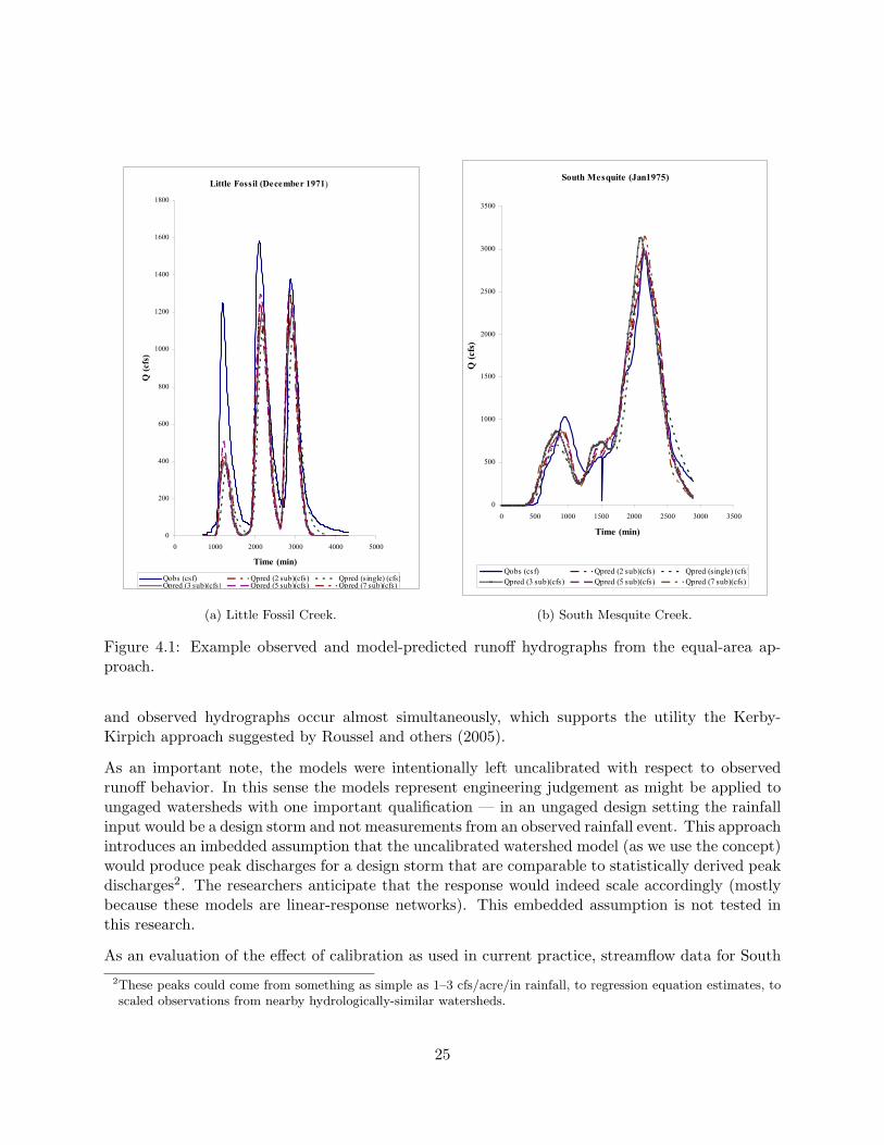
Examples of observed and model-predicted runoff hydrographs are presented in Figure 4.1. In caseswhere model-predicted runoff hydrographs approximate observed runoff hydrographs, there is noapparent substantial difference between the hydrographs. However, in many cases, the hydrographsgenerated by the model did not even approach observed results.

For example, the model hydrograph from South Mesquite Creek of January 1975 (Figure 4.1b)reasonably approximates the observed runoff hydrograph. However, the hydrographs from LittleFossil Creek of December 1971 (Figure 4.1a) are significantly different, particularly for the first hy-drograph of the series. Moreover, there is little difference between the simulated runoff hydrographsfor the subdivision and the single basin schemes and the observed hydrographs. The researchersspeculate that the reason for this particular result is that the spatial variability of the watershedis insufficient for the simulation results to be sensitive to the selected subdivision scheme1.

The use of soil type and land-use properties to determine spatial variability in the runoff generationcomponent of a hydrologic model is plausible because they (soil type, land-use) are the major factorsused to estimate runoff curve numbers, which were used in this application of HEC-HMS to estimaterunoff volume. In this research, the NRCS runoff curve number approach was used as the runoff

1This finding was the motivation behind Wingfield’s (2008) component in an attempt to test this hypothesis.

22

Table 4.1: Peak discharge analysis from equal-area subdivision approach (Luong, 2008). [Metric isthe method used to measure the difference between modeled and observed peak discharge, Numberof Subdivisions is the number of equal-area subdivisions for the study watershed, Selected is thenumber of equal-area subdivisions selected as providing the minimum error between modeled andobserved peak discharge, and Count is the number of events for which a given subdivision schemeperforms “better” than the other schemes tested. Xd and RMSE are expressed in percent.]

Watershed Metric Number of Subdivisions Selected1 2 3 5 7

Onion Xd −200 −285 −325 −282 −331 1RMSE 233 294 367 313 368 1Count 2 0 0 0 0 1

South Mesquite Xd 10 −5 −16 −28 −9 2RMSE 16 12 21 33 15 2Count 2 3 1 0 0 2

Little Fossil Xd −79 −99 −85 −123 −98 1RMSE 190 215 203 258 225 1Count 5 2 0 2 0 1

Olmos Xd −244 −241 −247 −149 −262 5RMSE 334 331 368 240 382 5Count 0 0 1 6 0 5

Trinity North Xd −14 −23 −18 −29 −10 7RMSE 72 73 68 74 63 7Count 2 0 0 3 4 7

generation model with HEC-HMS to compute runoff volumes. Alternative runoff-generation modelsare available (and implemented in HEC-HMS), but generally appeal to similar descriptive information.

In this study, the area-weighted mean curve number was almost identical across a watershed forall sub-watershed scenarios. As a result, there was little variation in the total runoff volumesbetween the sub-watershed configurations. The curve number for every unique soil and land-usecombination in the study watersheds was estimated assuming good hydrologic condition; however,this condition might not be true for all watersheds. Until the appropriate runoff-generation processmodel for the sub-watershed is accurately determined and incorporated into models, the resultsmay never be satisfactory.

In most cases, when hydrographs of subdivision are compared to the single basin, the patternof peak discharge is similar to the finding in earlier studies. The peak discharge for a lumpedwatershed is less than the peak discharge from the subdivided watershed. However, the magnitudeof the change in computed peak discharge changed little between the lumped and the subdividedscenarios in most cases, indicating that the peak flow component is relatively insensitive to changesin the number of sub-watersheds. This result implies that the model-predicted runoff is not heavilydependent on the degree of watershed subdivision. These findings are consistent with the resultsof Bingner and others (1997), FitzHugh and Mackay (2000), and Jha and others (2004).

Also, regardless of subdivision, with the exception of few storms, the peak discharges in simulated

23

Table 4.2: Time to peak discharge analysis from equal-area subdivision approach (Luong, 2008).[Metric is the method used to measure the difference between modeled and observed peak discharge,Number of Subdivisions is the number of equal-area subdivisions for the study watershed, Selectedis the number of equal-area subdivisions selected as providing the minimum error between modeledand observed peak discharge. Xd and RMSE are expressed in percent.]


Onion Xd −27 −23 −19 −30 −25 3RMSE 33 25 23 32 27 3Count 0 0 2 0 0 3

South Mesquite Xd −3 −2 0 −3 −4 3RMSE 9 10 8 11 12 3Count 1 1 1 1 2 7



Trinity North Xd −9 −9 −14 −14 −11 1RMSE 31 31 34 35 33 1Count 4 3 1 0 1 1

Table 4.3: Runoff volume analysis from equal-area subdivision approach (Luong, 2008). [Metric isthe method used to measure the difference between modeled and observed peak discharge, Numberof Subdivisions is the number of equal-area subdivisions for the study watershed, Selected is thenumber of equal-area subdivisions selected as providing the minimum error between modeled andobserved peak discharge. Xd and RMSE are expressed in percent.]


Onion Xd −520 −432 −465 −467 −466 2RMSE 663 538 587 589 587 2Count 0 1 1 0 0 2, 3

South Mesquite Xd −4 −6 −1 0 0 7RMSE 22 19 17 17 16 7Count 3 1 1 1 0 1



Trinity North Xd −33 −20 −20 −18 −18 5RMSE 88 73 69 68 68 5Count 0 1 4 4 0 3, 5

24

45

model did not reproduce runoff volume close to observed results (unfavorable predictions).

Little Fossil (December 1971)

0

200

400

600

800

1000

1200

1400

1600

1800

0 1000 2000 3000 4000 5000

Time (min)

Q (

cfs

)

Qobs (csf) Qpred (2 sub)(cfs) Qpred (single) (cfs)Qpred (3 sub)(cfs) Qpred (5 sub)(cfs) Qpred (7 sub)(cfs)

Figure 4.1. Simulated and observed hydrographs (Little Fossil 12/1971)

(a) Little Fossil Creek.

47

South Mesquite (Jan1975)

0

500

1000

1500

2000

2500

3000

3500

0 500 1000 1500 2000 2500 3000 3500

Time (min)

Q (

cfs

)

Qobs (csf) Qpred (2 sub)(cfs) Qpred (single) (cfs)

Qpred (3 sub)(cfs) Qpred (5 sub)(cfs) Qpred (7 sub)(cfs)

Figure 4.3. Simulated and observed hydrographs (South Mesquite 1/1975) (b) South Mesquite Creek.

Figure 4.1: Example observed and model-predicted runoff hydrographs from the equal-area ap-proach.

and observed hydrographs occur almost simultaneously, which supports the utility the Kerby-Kirpich approach suggested by Roussel and others (2005).

As an important note, the models were intentionally left uncalibrated with respect to observedrunoff behavior. In this sense the models represent engineering judgement as might be applied toungaged watersheds with one important qualification — in an ungaged design setting the rainfallinput would be a design storm and not measurements from an observed rainfall event. This approachintroduces an imbedded assumption that the uncalibrated watershed model (as we use the concept)would produce peak discharges for a design storm that are comparable to statistically derived peakdischarges2. The researchers anticipate that the response would indeed scale accordingly (mostlybecause these models are linear-response networks). This embedded assumption is not tested inthis research.

As an evaluation of the effect of calibration as used in current practice, streamflow data for South2These peaks could come from something as simple as 1–3 cfs/acre/in rainfall, to regression equation estimates, toscaled observations from nearby hydrologically-similar watersheds.

25

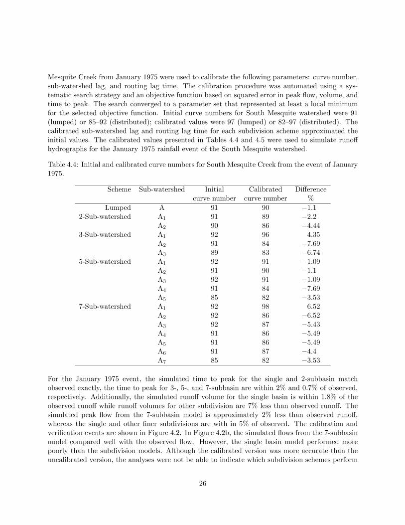
Mesquite Creek from January 1975 were used to calibrate the following parameters: curve number,sub-watershed lag, and routing lag time. The calibration procedure was automated using a sys-tematic search strategy and an objective function based on squared error in peak flow, volume, andtime to peak. The search converged to a parameter set that represented at least a local minimumfor the selected objective function. Initial curve numbers for South Mesquite watershed were 91(lumped) or 85–92 (distributed); calibrated values were 97 (lumped) or 82–97 (distributed). Thecalibrated sub-watershed lag and routing lag time for each subdivision scheme approximated theinitial values. The calibrated values presented in Tables 4.4 and 4.5 were used to simulate runoffhydrographs for the January 1975 rainfall event of the South Mesquite watershed.

Table 4.4: Initial and calibrated curve numbers for South Mesquite Creek from the event of January1975.

Scheme Sub-watershed Initial Calibrated Differencecurve number curve number %

Lumped A 91 90 −1.12-Sub-watershed A1 91 89 −2.2

A2 90 86 −4.443-Sub-watershed A1 92 96 4.35

A2 91 84 −7.69A3 89 83 −6.74

5-Sub-watershed A1 92 91 −1.09A2 91 90 −1.1A3 92 91 −1.09A4 91 84 −7.69A5 85 82 −3.53

7-Sub-watershed A1 92 98 6.52A2 92 86 −6.52A3 92 87 −5.43A4 91 86 −5.49A5 91 86 −5.49A6 91 87 −4.4A7 85 82 −3.53

For the January 1975 event, the simulated time to peak for the single and 2-subbasin matchobserved exactly, the time to peak for 3-, 5-, and 7-subbasin are within 2% and 0.7% of observed,respectively. Additionally, the simulated runoff volume for the single basin is within 1.8% of theobserved runoff while runoff volumes for other subdivision are 7% less than observed runoff. Thesimulated peak flow from the 7-subbasin model is approximately 2% less than observed runoff,whereas the single and other finer subdivisions are with in 5% of observed. The calibration andverification events are shown in Figure 4.2. In Figure 4.2b, the simulated flows from the 7-subbasinmodel compared well with the observed flow. However, the single basin model performed morepoorly than the subdivision models. Although the calibrated version was more accurate than theuncalibrated version, the analyses were not be able to indicate which subdivision schemes perform

26

Table 4.5: Initial and calibrated timing parameters for South Mesquite Creek from the event ofJanuary 1975.

Scheme Sub-watershed Initial Calibrated Differencetreach treach %

Lumped A2-Sub-watershed A1

A2 217 250 15.213-Sub-watershed A1

A2 91 92 1.1A3 173 174 0.58

5-Sub-watershed A1

A2 72 73 1.39A3 57 40 −29.82A4 123 141 14.63A5 129 125 −3.1

7-Sub-watershed A1

A2 80 81 1.25A3 68 69 1.47A4 76 77 1.32A5 90 91 1.11A6 89 90 1.12A7 90 91 1.11

best. Furthermore, the hydrographs generated using the uncalibrated and calibrated models arepractically indistinguishable. Therefore, changes of a few percent in globally-applied values havelittle effect on the simulations. Finally, in many practical instances such calibration is unrealisticbecause the requisite data simply do not exist.

Runoff hydrographs that were developed for the Onion Creek, South Mesquite, Little Fossil, OlmosCreek, and Trinity Basin-North watersheds were used in similar analyses to determine the effectsthat sub-watershed count had on the runoff hydrographs. The increase in the sub-watershed countdoes not substantially affect the simulated runoff hydrograph.

In Luong’s study (2008), neither peak flows nor runoff volumes were simulated accurately fromindividual events, regardless of subdivision scheme. However, results of predicted time to peakwere somewhat better.

Unless there is some compelling need to divide a watershed into smaller pieces, compute the dis-charge from those pieces, route those discharges to the outlet, and compute a total discharge, thereis little if any gain in “accuracy.” Compelling needs fall into only a few categories: (i) a huge changein watershed runoff generation is anticipated on a portion of the total watershed (both the changeand the portion need to be substantial), (ii) a huge change in routing time is anticipated (perhapsby ditch building over considerable distances), (iii) a regulation effect is anticipated on a portion of

27

55

South Mesquite (Jan1975)

0

500

1000

1500

2000

2500

3000

3500

0 500 1000 1500 2000 2500 3000 3500

Time (min)

Q (

cfs

)



Figure 4.5. Simulated and observed hydrographs (South Mesquite 1/1975-Calibrated)

(a) Calibration event.

56

South Mesquite (March 1977)

0

1000

2000

3000

4000

5000

6000

0 1000 2000 3000 4000 5000

Time (min)

Q (

cfs

)



Figure 4.6. Simulated and observed hydrographs (South Mesquite 3/1977-Calibrated)

(b) Verification event.

Figure 4.2: Calibration and verification events for South Mesquite Creek from the events of January1975 and March 1977.

the watershed (a reservoir being an extreme example), (iv) a huge change in on-watershed storageis anticipated (a subset of a reservoir case, or (v) there is a large change in slope (such as thewatershed traversing across an escarpment — this is a special case of (ii)).

The general cases outlined in the previous paragraph are the compelling physical structures wheresubdivision would make sense — the cases are beyond what a lumped model could explain a priori3.

These cases could justify subdivision in order to answer “what-if” questions. But improved “ac-curacy” in the absence of these demarkations is not justification for breaking a model into smallerparts.

The result of this component, and the conjectures in the above paragraph stimulated the Wing-field (2008) study to address “How big of a change is needed to impact the computed outputhydrograph?”

3A lumped model could be forced to fit observations, but the researchers’ opinion is that the various terms couldnot be explained beforehand.

28

4.2. Lumped Models

4.2.1. Watershed Subdivision

The first objective of the lumped-model component of this research was to apply ArcHydro andHEC-GeoHMS to delineate the five study watersheds and to extract modeling parameters for eachone. Once this was completed, the five study watersheds were subdivided into 3, 5, 7, 10, 15, and30 sub-watersheds. ArcGIS was used to develop modeling parameters for the sub-watersheds.

The relative error between computed and observed runoff volume for the Walnut Creek studywatershed is displayed on Figure 4.3. The impact of watershed subdivision on computed runoffvolume is minor. This result is attributable to the fact that the runoff potential, as representedby the NRCS curve number method, is not sensitive to watershed subdivision. Results for WalnutCreek are representative of relative errors in runoff volume for the remaining watersheds in thestudy dataset.

Figure 4.3: Runoff volume relative error for Walnut Creek study watershed.

The relative error for peak discharge is displayed on Figure 4.4. The tendency is for the relativeerror in peak discharge to decrease with the number of watershed subdivision. However, afterbetween 5 and 10 subdivisions, no additional reduction in the relative error in peak discharge isobtained.

The time to peak discharge from the study events was extracted from both the modeled andobserved hydrographs. Results from computation of the relative errors are displayed on Figure 4.5.With the exception of results from Pond-Elm Creek, the accuracy of time to peak estimates tendto decrease with increasing number of subdivisions.

29

(a) Walnut Creek.

(b) Ash Creek.

(c) South Mesquite Creek.

(d) Calaveras Creek.

(e) Pond-Elm Creek.

Figure 4.4: Relative error in peak discharge for study watersheds.

30

(a) Walnut Creek.

(b) Ash Creek.


(d) Calaveras Creek.

(e) Pond-Elm Creek.

Figure 4.5: Relative error in peak discharge for study watersheds.

31

As the number of watershed subdivisions increases, the complexity of the stream network used toconnect the sub-watershed outlets increases. For each stream segment in the network, a number ofparameters are required to route the sub-watershed hydrographs. That is, each stream segment hasa set of routing parameters associated with it and each of these parameters must be estimated. Fora relatively simple routing approach, such as simply lagging the input hydrograph in time, the num-ber of required routing parameters increases roughly linearly with the number of sub-watersheds.However, errors in the routing-parameter estimates are reflected in the output hydrograph fromthe watershed.

For example, the observed and computed runoff hydrographs for the event of October 20, 1984on Walnut Creek are presented on Figure 4.6. For three subdivisions, the computed runoff hy-drograph becomes bimodal. Although there is some indication of the impact of a second pulseof effective rainfall evident in the observed hydrograph (the small “hump” on the recession limb),the pronounced bimodal computed hydrograph is indicative that the routing algorithm is eithermis-specified or the routing parameters are not correct.

Figure 4.6: Runoff hydrographs from the event of October 20, 1984 on Walnut Creek.

Without an observed hydrograph for calibration, an analyst would have no idea whether the resultsdepicted on Figure 4.6 are correct. The authors would suspect that a problem existed and any expertcould “correct” the problem such that the computed hydrograph would be unimodal, as expected.However, without an observed hydrograph for calibration, it could not be known whether therouting sub-model was correctly specified or whether the parameters were reasonable, much less“correct.”

The point is that when watershed are subdivided, the number of parameters increases more quicklythan the number of sub-watersheds. The proliferation of parameters is a problem. Without mea-surements to use in calibrating the parameters, it is difficult to set those values to anything other

32

than “average” or representative values, which results in the paradox. This issue was discussedat length by Hornberger and others (1985) and Jakeman and Hornberger (1993) and many otherresearchers who examined the complexity of watershed models during the 1980s.

For example, if a single watershed unit modeling using HEC-HMS requires three parameters4, then asingle subdivision (two sub-watersheds) would require estimates for six parameters for the rainfall-runoff model and at least two more for a routing sub-model. The required number of parameterestimates scales from that point. The problem is exacerbated if another runoff-generation processmodel (such as initial-abstraction/constant loss-rate or Green-Ampt) is used in place of the runoffcurve number method.

4.2.2. Changes to Parameter Values

The second component of the lumped-model component of this research was to examine the impactthat radical changes to parameter values for a subdivision (or subdivisions) of a watershed mighthave on the computed runoff hydrograph from the watershed. That is, the objective was to askthe question “What is the impact on the runoff hydrograph from the watershed if parameter x ischanged by a ridiculous amount?”, then adjust lumped-model parameters for various fractions ofthe total watershed drainage area and re-run the HEC-HMS models.

The runoff curve number was adjusted from the starting value to 100 for fractions of about 1/5,1/3, and 1/2 of the total watershed area (denoted by 1/5CN, 1/3CN, and 1/2CN on the figures).The basin lag time was arbitrarily reduced by 20 percent for the same 1/5, 1/3, and 1/2 of thetotal watershed area (but in an independent set of HEC-HMS models; denoted by 1/5lag, 1/3lag, and1/2lag on the figures). Finally, the routing lag time was decreased by 20 percent for about 1/5,1/3, and 1/2 of the watershed drainage area (denoted by 1/5Rout, 1/3Rout, and 1/2Rout on thefigures).

Results of the indicated changes to lumped-model parameter values are presented on Figures 4.7–4.11. With the exception of the models for Calaveras Creek, a change from the base parametervalues to extreme parameter values (curve number of 100, 20 percent decrease in basin lag timeor reach routing time) resulted in computed results that were within one-third log cycle of thebase peak discharge from the watershed runoff hydrograph. Therefore, there must be a markedlydifferent parameter value (or values) for a sub-watershed to justify subdivision on the basis ofrepresenting differences in parameter values by watershed subdivision.

The use of one-third log cycle as a discrimination range is a value that the researchers noticed iscommon in their recent work. The researchers believe that this range (one-third of a log cycle)represents current technological ability to discriminate differences5, and that it would be difficultto discriminate using a statistical test with a reasonable level of significance between two modelsthat produce responses within one-third of a log cycle. Therefore, any of the models for the Walnut

4Typical parameters used in a HEC-HMS model are lag time, runoff curve number, and percent impervious area.5For example, the standard error of estimate for the regional regression equations for Texas, Asquith and Thompson(2005, 2008), and Asquith and others (in press), is about 40 percent, which approximates one-third of a log cycle.

33

Creek, South Mesquite Creek, or Pond Elm Creek watersheds would perform about the same(barely escape the range). More diagnostic is which changes matter more — in runoff volume thegeneration model is important, and that importance is indeed reflected by results presented in thegraphs. Lesser sensitivity occurs with the other important responses, peak discharge and time topeak. The relative insensitivity (change in response related to change in parameter) in these limitedstudies supports the contention that arbitrary subdivision with only subtle variation in watershedparameters is not useful.

Figure 4.7: The impact of extreme parameter changes on the runoff hydrograph from WalnutCreek. Marks denote changes to hydrograph runoff volume resulting from the indicated change inparameter value. Error bars denote range corresponding to one-third of a log cycle.

34

Figure 4.8: The impact of extreme parameter changes on the runoff hydrograph from Ash Creek.Marks denote changes to hydrograph runoff volume resulting from the indicated change in param-eter value. Error bars denote range corresponding to one-third of a log cycle.

Figure 4.9: The impact of extreme parameter changes on the runoff hydrograph from SouthMesquite Creek. Marks denote changes to hydrograph runoff volume resulting from the indicatedchange in parameter value. Error bars denote range corresponding to one-third of a log cycle.

35

Figure 4.10: The impact of extreme parameter changes on the runoff hydrograph from CalaverasCreek. Marks denote changes to hydrograph runoff volume resulting from the indicated change inparameter value. Error bars denote range corresponding to one-third of a log cycle.

Figure 4.11: The impact of extreme parameter changes on the runoff hydrograph from Pond-ElmCreek. Marks denote changes to hydrograph runoff volume resulting from the indicated change inparameter value. Error bars denote range corresponding to one-third of a log cycle.

36

4.3. Distributed Models

ArcHydro and GeoHMS were used to develop distributed hydrologic models using the gridded modelfeature of HEC-HMS (U.S. Army Corps of Engineers, 2008). The three study watersheds (Ash Creek,Pond-Elm Creek, and South Mesquite Creek) were subdivided into 1 (no subdivision), 2, 3, 5, 7,and 9 sub-watersheds using an approach where the watershed was subdivided at locations thatprovided sub-watersheds of approximately equal drainage area. However, sub-watershed drainageareas could not be forced to be strictly equal; a tolerance of about ten percent was used.

The resulting suite of watershed models6 were operated and results extracted. Relative errors(arithmetic mean and root mean squared errors) were computed using Equations 2.8 and 2.9. Aplot of the relative errors of runoff volume as a function of the number is subdivisions is presented inFigure 4.12. A pattern similar to that observed using the lumped-modeling approach (Figure 4.3)is evident. Little change in runoff volume occurs based on the number of watershed subdivisions.This occurs because the runoff curve number is not sensitive to watershed subdivision.

Estimates of peak discharge were extracted from the model results and the relative errors werecomputed. The relative errors are displayed on Figure 4.13. A moderate change in the relativeerrors occurred with an increasing number of subdivisions. When the mean relative error is usedas a metric, predicted peak discharge was less accurate with increasing subdivision of the studywatersheds. Furthermore, the RMSE for only South Mesquite Creek improved with increasingsubdivision.

The modeled time to peak discharge was extracted from the model output and relative errors werecomputed. The relative errors are presented on Figure 4.14. Estimates of time to peak from thesubdivided model worsened with increasing subdivision of the study watersheds.

An example hydrograph from the March 27, 1977 runoff event from Ash Creek is displayed onFigure 4.15. A significant error in the uncalibrated modeled time to peak discharge is evident.The secondary watershed response is amplified in the model-predicted runoff hydrograph, whichprobably indicates that the measured rainfall hyetograph does not represent the actual spatialdistribution of event rainfall. Furthermore, the impact of subdivision on routing through thewatershed drainage network is evident from the changes in hydrograph timing that occur withincreasing watershed subdivision. This finding is similar to that observed with the lumped-modelingapproach and reinforces observations about the increasing importance of hydrologic routing as thelevel of watershed subdivision increases.

6It must be emphasized that a tremendous amount of work was required to develop the basin models using ArcHydro

and GeoHMS.

37

‐40%‐30%‐20%‐10%0%10%20%30%40%50%

0 2 4 6 8 10

Rela%veErrorinRun

offVolum

e(%

)

NumberofSubdivisions

AshCreek‐RunoffVolumeModeledv.Observed

Arithme3cMean

RRMSE

(a) Ash Creek.

‐40%

‐20%

0%

20%

40%

60%

0 2 4 6 8 10

Rela%veErrorinRun

offVolum

e(%

)


Li;lePondElmCreek‐RunoffVolumeModeledv.Observed

Arithme1cMean

RRMSE

(b) Little PondElm Creek.

‐40%

‐20%

0%

20%

40%

60%

0 2 4 6 8 10

Rela%veErrorinRun

offVolum

e(%

)


SouthMesquiteCreek‐RunoffVolumeModeledv.Observed

Arithme1cMean

RRMSE


Figure 4.12: Relative errors of runoff volume as a function of the number of subdivisions fromdistributed modeling.

38

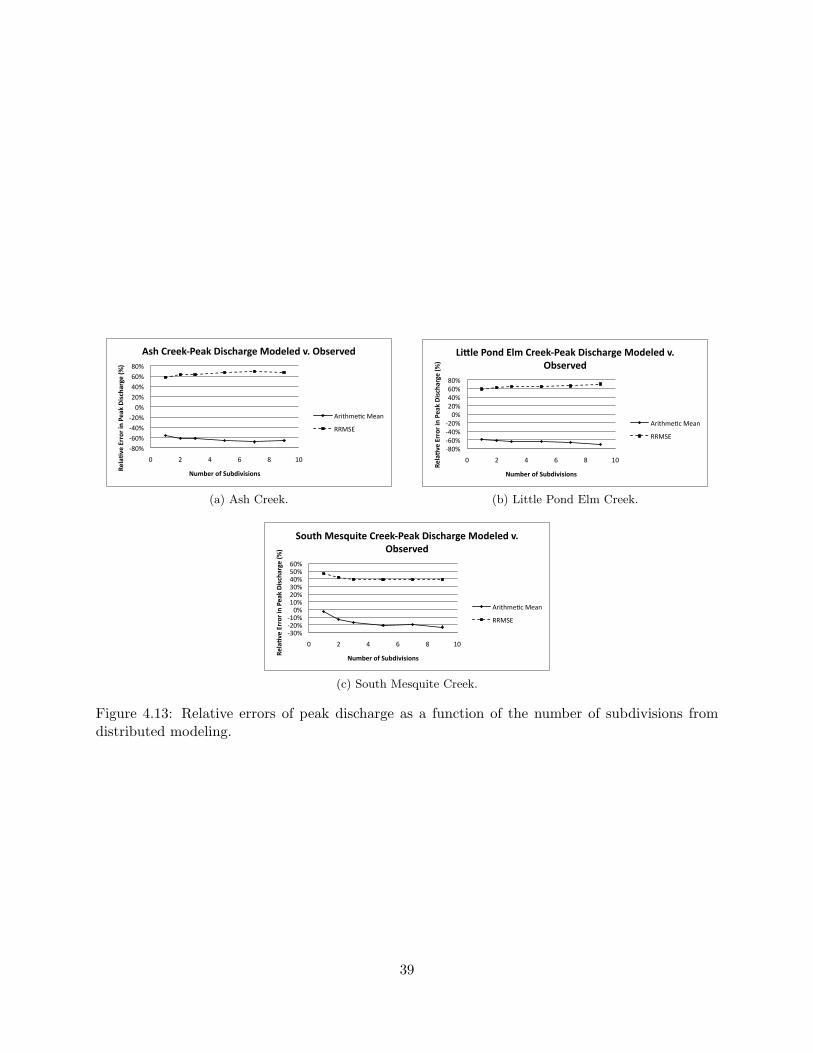
‐80%‐60%‐40%‐20%0%20%40%60%80%

0 2 4 6 8 10

Rela%veErrorinPeakDischarge(%

)


AshCreek‐PeakDischargeModeledv.Observed

Arithme1cMean

RRMSE

(a) Ash Creek.

‐80%‐60%‐40%‐20%0%20%40%60%80%

0 2 4 6 8 10


)


Li?lePondElmCreek‐PeakDischargeModeledv.Observed

Arithme1cMean

RRMSE

(b) Little Pond Elm Creek.

‐30%‐20%‐10%0%10%20%30%40%50%60%

0 2 4 6 8 10


)


SouthMesquiteCreek‐PeakDischargeModeledv.Observed

Arithme3cMean

RRMSE


Figure 4.13: Relative errors of peak discharge as a function of the number of subdivisions fromdistributed modeling.

39

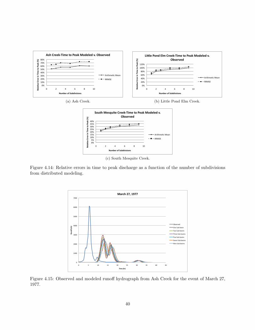
0%10%20%30%40%50%60%70%80%

0 2 4 6 8 10Rela%veErrorinTim

etoPeak(%

)


AshCreek‐TimetoPeakModeledv.Observed

Arithme3cMean

RRMSE

(a) Ash Creek.

0%

20%

40%

60%

80%

100%

120%


etoPeak(%

)


Li=lePondElmCreek‐TimetoPeakModeledv.Observed

Arithme0cMean

RRMSE

(b) Little Pond Elm Creek.

0%5%10%15%20%25%30%35%40%


etoPeak(%

)


SouthMesquiteCreek‐TimetoPeakModeledv.Observed

Arithme2cMean

RRMSE


Figure 4.14: Relative errors in time to peak discharge as a function of the number of subdivisionsfrom distributed modeling.

0

1000

2000

3000

4000

5000

6000

7000

0 5 10 15 20 25 30 35 40 45

Runo

ff(cfs)

Time(hr)

March27,1977

Observed

OneSub‐basin

TwoSub‐basins

ThreeSub‐basins

FiveSub‐basins

SevenSub‐basins

NineSub‐basins

Figure 4.15: Observed and modeled runoff hydrograph from Ash Creek for the event of March 27,1977.

40

4.4. Stochastic Modeling

Two numerical experiments were conducted using a highly-complex, single-purpose suite of pro-gramming tools written in the R language (R Development Core Team, 2006). These tools arecollectively referred to as GUHtools and are anticipated to be available for download from thehome page of Asquith and Roussel (2007). These tools allow simulation of IA, CL, Tp, Qp, and X,and combine various intermediate computations to yield a simulated hydrograph given the inputprecipitation identified previously. These tools also accommodate vector summation to superim-pose hydrographs and routed hydrographs using route length H as necessary to mimic a watershedsubdivision scenario.

The two numerical experiments, that is, the configuration and properties of the sub-watersheds,are as follows:

1. Two undeveloped (D = 0) sub-watersheds with A = 12 = Ao/2 and L = 3 = Lo/2 weresimulated in which one watershed cascades into the second and therefore the length ofrouting for the upstream watershed through the downstream watershed is 3 miles or H = 3.

2. Two developed (D = 1) sub-watersheds with A = 12 = Ao/2 and L = 3 = Lo/2 weresimulated in which one watershed cascades into the second and therefore the length ofrouting for the upstream watershed through the downstream watershed is 3 miles or H = 3.

For both simulation experiments, all other watershed characteristics matched those of the wholewatershed. In order to compute Qi(AR)

p the whole watershed was simulated for D = 0 or D = 1depending on which experiment was conducted.

In an unsophisticated fashion, values of ck (ck | 1 → 2 : ∆ck = 0.05) were systematically incre-mented (each value used) and 2,000 simulations per loop made. The resulting values for ε for eachck by experiment were retained. The results are depicted on Figures 4.16 and 4.17. From thefigures, the values for η are determined by inspection of the generalized location of the minimum ofthe ε(ck) values and are approximately 1.05 and 1.6 for the undeveloped and developed watersheds,respectively.

41

CELERITY FACTOR (η ) FOR ck ∝ η(L/Tc), DIMENSIONLESS

PEAK

STRE

AMFL

OWER

ROR,

INCU

BIC

FEET

PER

SECO

ND

TIM

EOF

PEAK

ERRO

R,IN

HOUR

S

0.5 0.6 0.8 1 1.2 1.4 1.5-100

0

100

200

300

400

500

600

700

-1.12

-1.10

-1.08

-1.06

-1.04

-1.02

-1.00

-0.98

-0.96

Peak streamflow error ε = |E[Qi(route)p ]−E[Qi(AR)

p ]|Time of peak error E[T Qp(route)]−E[T QpAR]

EXPLANATION

Undeveloped watersheds

Figure 4.16: Relation between absolute value of peak streamflow error and celerity factor for twocascading undeveloped sub-watersheds.

42

CELERITY FACTOR (η ) FOR ck ∝ η(L/Tc), DIMENSIONLESS

PEAK

STRE

AMFL

OWER

ROR,

INCU

BIC

FEET

PER

SECO

ND

TIM

EOF

PEAK

ERRO

R,IN

HOUR

S

1 1.2 1.4 1.6 1.8 2-100

0

100

200

300

400

500

600

700

-0.39

-0.38

-0.37

-0.36

-0.35

-0.34

-0.33

-0.32

-0.31

-0.30

-0.29

Peak streamflow error ε = |E[Qi(route)p ]−E[Qi(AR)

p ]|Time of peak error E[T Qp(route)]−E[T QpAR]

EXPLANATION

Developed watersheds

Figure 4.17: Relation between absolute value of peak streamflow error and celerity factor for twocascading developed sub-watersheds.

43

The results of the numerical experimentation described in Section 2.5 suggest that η(D=0) ≈ 1.05and that η(D=0) ≈ 1.6. From which, following Equation 2.11 we can express ck as

ck ≈

{1.05L[feet]/(T [seconds]

p /0.7) for D = 01.6L[feet]/(T [seconds]

p /0.4) for D = 1,(4.1)

or after simplification

ck ≈

{0.74L[feet]/T

[seconds]p for D = 0

0.64L[feet]/T[seconds]p for D = 1.

(4.2)

Combining the two η values by averaging through justification that η represents something innateto hydraulics, we get a generalized η = 0.69, which following the structure of Equation 4.2, yields

ck ≈ 0.69(L[miles] × 5280)

(T [hours]p × 3600)

, (4.3)

where unit conversion factors have been introduced, ck is celerity in feet per second, L is main-channel length in miles, and Tp is time to peak in hours. Emphasis again is needed that L is not arouting length H, but is the main-channel length of the sub-watershed from which streamflow willbe routed R distance downstream. Upon further simplification units, we get

ck ≈ 1.01L

Tp→ ck ≡

L

Tp, (4.4)

which is an appropriate generalization given substantial fraction of log10-cycle errors seen in esti-mation of IA, CL, Tp, qp, and X.

Asquith and Roussel (2007) established that

Tp = 10−1.49−0.354DL0.602S−0.672. (4.5)

Therefore, with substitution, ck can be directly computed by observing that the equivalency ck ≡L/Tp, which is established in Equation 4.4, yields

ck = 101.49+0.354DL0.398S0.672, (4.6)

where the variables are previously defined. The equation is interpreted as follows:

• Developed D = 1 watersheds have higher ck than undeveloped D = 0 watersheds,

• As S increases ck increases, and

• As L increases ck increases.

The response of ck to S is obviously consistent with expectation of fundamental open-channel hy-draulics. The response of ck to D could be indicative of the more “urban” nature of the channels

44

(stabilized, lined, sewer, other utility co-location. . . ) intrinsically represented in the D = 1 wa-tersheds of available to the research team. Finally, the fact that Equation 4.6 shows ck increasingwith increasing L is more difficult to interpret other than acknowledging that as L increases the Sfor a watershed generally decreases. Perhaps some compensation between the two characteristicsoccurs.

Based on these results, ck can be estimated through Equation 4.6 for an arbitrary watershed insuch a fashion as to constrain an important parameter in hydraulic routing to produce Qp valuesthat are generally consistent with values that would be produced by treating the watershed as alumped system through the Asquith and Roussel (2007) procedures. This is an important finding aseither some constraint on values for ck or some estimate of ck can be made from purely hydrologicanalysis. Another contribution of the experimental approach is that the relation between Tp andTc as shown in Roussel and others (2005, p. 15) define a situation in which the η could be treatedas a constant for undeveloped and developed watersheds.

4.4.1. Example Computation

Suppose that a hydrograph is to be routed a distance H downstream from a 6-square mile, undevel-oped, and rock-dominated R = 1 watershed with a main-channel length of 4 miles, a dimensionlesschannel slope of 0.009, and a curve number of CN = 65. What Muskingum routing parametersshould be used? Given that no other information is provided, it is suggested that X ≈ 0.2 be usedas this value seems representative from discussion in engineering textbooks. The values for R andCN are not part of the solution to the question. The celerity ck = 101.49+0.354(0)40.398(0.009)0.672

or about 2.3 feet per second.

If the watershed were to become developed, what is the estimate for ck? Substitution yieldsck = 101.49+0.354(1)40.398(0.009)0.672 or about 5.1 feet per second

4.4.2. Caveats

Final caveats are needed. Although providing potentially valuable insight in to the problem ofparameterizing a component of the Muskingum routing for a subdivided watershed, the exper-iments reported here constitute an elementary example of watershed subdivision. The authorsexperimented with multiple levels of cascading subdivisions and similar behavior for η value andthe minimization of ε were seen.

The authors attempted, through stochastic simulation, to retain uncertainty and mitigate for po-tential nonlinearities caused by the discontinuous nature of the initial-abstraction, constant-lossmodel of watershed losses. It is difficult to assess the full reliability of the numerical computations;although various intermediate visualizations of hydrographs were used in development of the algo-rithms. The authors used mutually independent simulations of all characteristics; this is likely notan appropriate method but further assessment is well beyond the scope of this research project.Also the authors do not address the question of how large a reach length for routing should be.

45

The authors recognize that it is entirely possible that the generalized η = 0.67 in Equation 4.3is in fact not generalizable and therefore not a constant. If such a situation could be shown byother configurations of stochastic experiments as described here or by real-world data, then thewatershed subdivision problem is exceptionally difficult to simplify7 and preference to lumped-parameter models, such as that described in Asquith and Roussel (2007), should be made lackingspecific information about the hydraulics of a channel system.

7In the absence of sufficient geometric, topographic, and topologic information to specify channel hydraulics (in-cluding underground engineered drainage networks) generalizations or just plain engineering guesses are a logicalstep to configure uncalibrated subdivided models. Such generalizations could be interpreted as a style of lumped-parameter modeling, much in the same vein that modeling itself is really a sophisticated from of regression. Theintellectual controversy of this point of view notwithstanding, the authors lean to lumped-parameter models whenchannel system hydraulics are poorly characterized and when the subdivision is a relatively arbitrary choice.

46

5. Summary and Conclusions

The purpose of this chapter is to provide a summary of research work accomplished and a synopsisof the research findings. In addition, suggestions for further research into issues associated withwatershed modeling, in general, and subdivision of watersheds for modeling are provided.

TxDOT engineers and consultants to TxDOT are tasked with hydrologic modeling of watershedsto provide estimates of design discharges. The resulting design discharge estimates are then usedto size hydraulic structures for Texas highways. Inevitably, working with watersheds is a requiredcomponent of this modeling. The objectives for TxDOT Research Project 0–5822, Subdivision ofwatersheds for hydrologic modeling were:

1. Determine justification and methodology for subdividing watersheds for use with lumpedmodels, and

2. Assess the utility of distributed models, such as the gridded sub-model system of HEC-HMS.

Based on the literature review, the general consensus of the researchers is that simpler is better.That is, the principle of parsimony1 is wise. In this context, parsimony refers to an conceptualizationof watershed behavior that depends on the least complex assembly of model components. Thatis, watershed models should generally not be subdivided any more than necessary to obtain aconceptual representation that reflects the physical reality of the system. Subdivision does notresult in improved “accuracy” and should not be used with the assumption that results fromsubdivided watershed models are somehow superior to topologically-simpler models.

Watersheds should not be arbitrarily subdivided; additional subdivision does not result in improved“accuracy.” Subdivision to accommodate (i) a huge change in watershed runoff generation on asubstantial portion ( 1/3) of the total watershed, (ii) a huge change in routing time (perhaps byditch building over considerable distances), (iii) a regulation effect on a portion of the watershed(a reservoir being an extreme example), (iv) a huge change in on-watershed storage, or (v) alarge change in slope (such as the watershed traversing across an escarpment), makes sense andthese physical situations demand such consideration. The analyst will need to be aware thatsuch subdivision increases the parameter count. Furthermore, if subdivision is applied the modelhas to route flows — the selection of routing parameters becomes exceedingly important and theuncertainty in the timing parameters in a runoff hydrograph is transferred (and probably multiplied)to the uncertainty in the routing parameters.

1Also known as Occam’s Razor.

47

A few words about the concept of model calibration are required. When modelers use the termcalibration, the general intent is optimization of watershed-model parameter sets such that themeasured hydrograph response of a watershed is reproduced (in some objective sense) by thecalibrated model2. The process is similar in concept to application of least squares curve fittingin that an objective function (for example, the sum of the squared residuals) is minimized byadjusting model parameters. In the context of a watershed model, the resulting parameter sets mustpass the “reasonableness” test. That is, it is inappropriate to choose parameters that are beyondphysical justification simply to improve the fit of the model to the observations3. A substantialdegree of professional judgment is required to choose appropriate parameter values, even whenusing tools such as HEC-HMS to provide “best” parameter estimates. Finally, measured rainfall-runoff observations generally contain sufficient information to calibrate no more than about tenparameters (Hornberger and others, 1985).

Another approach is that watershed models (all models for that matter) should be compared toobservations if excitation-response data are available. In some instances, these observations can beused to adjust some of the model parameters with the caveat that the adjusted values should remainphysically realistic and appropriate for the system being modeled, an equally acceptable alternativeis to scale the response for the comparison. The first kind of “calibration” becomes thorny whenthe observation set is partitioned into a calibration component and a validation component — ifthe validation fails, then it (the validation set) has just become part of the calibration set and isno longer an independent partition.

Regardless of the end-user’s opinion about calibration, measured rainfall-runoff responses should beused to confirm model operation is such observation are available. Whether that approach takes theform of a parameter-optimization method or a scaling method is a matter of professional judgmentand remains in the purview of the analyst. The expectation, however, is that (1) it is impossible tofind a parameter set that reproduces the observed hydrograph for all rainfall-runoff events in thedatabase and such expectation on the part of the analyst is unreasonable, and (2) parameter sets(whether estimated or calibrated) must be within the realm of physical reasonability.

The research project was pursued through four avenues of study: (1) An iso-characteristic ap-proach, implemented as equal drainage area4; (2) an ad-hoc subdivision approach implementedas a professional would choose to subdivide a watershed based on professional experience; (3)a distributed-modeling approach, using HEC-HMS (U.S. Army Corps of Engineers, 2008) as themodeling tool; and (4) a stochastic-simulation approach to examine the channel travel-time forMuskingum routing. A variety of Texas watersheds for which measured rainfall-runoff responses(Asquith and others, 2004) were used to conduct the study. The degree of subdivision depended onthe method used to examine the impact of watershed subdivision. A maximum of 30 subdivisionswas used.

2This is in direct opposition to the notion that a desired computational result can be obtained by “tweaking” modelparameters. The latter approach is, at best, intellectually dishonest. The comedic consultant’s response “Whatwould you like the answer to be?” is a parody thereof.

3This is one of the reasons that the optimizer in HEC-HMS provides the capability to limit the search space forparameter values.

4Other iso-characteristic subdivision schemes include equal time of concentration, equal main channel slope, andequal overland flow slope. Basically, any physical watershed characteristic could be used.

48

Uncalibrated HEC-HMS models5 were developed for each of the watersheds in the study database.A no-subdivision model was included in each method tested. This model represented the simplestcase (no subdivision) in which all parameters are averaged (or lumped) for the watershed. Selectedrainfall-runoff events were used for each watershed model, the model was operated, and estimatesof runoff volume (watershed units), peak estimated discharge, and time to peak discharge wereextracted from model output. Relative errors between predicted and observed values were computedand are reported in Chapter 4.

In general, no change was observed in the estimation of runoff volume. This result is directlyattributable to use of the NRCS curve number method. However, unless the distribution of rainfall-runoff sub-process model parameters at sub-watershed scale is justified (and sufficient supportingdata actually exist or can be obtained), this result will hold true regardless of the rainfall-runoffsub-process model used.

The number of parameters requiring estimates increased as the number of subdivisions increased.The issue was exacerbated by introduction of required hydrologic routing to move computed hydro-graphs from internal sub-watershed outlets to the main watershed outlet. The number of routingparameters required depended on the choice of the hydrologic routing sub-process model and thenumber of elements chosen. In the simplest case, one “channel” was required to convey flows fromthe sub-watershed outlet to the next downstream confluence of sub-watersheds.

Examination of the travel-time parameter for Muskingum routing using a stochastic-modeling ap-proach was undertaken. Two simple watersheds were assumed, each comprising a cascade of twosub-watersheds — an upper sub-watershed and a lower sub-watershed. One set was assumed to beundeveloped and the second set was assumed to be developed. Estimates of peak discharge wereextracted using methods defined by Asquith and Roussel (2007) for the upstream and downstreamsub-watersheds, and for the watershed as a whole. The travel time (or wave celerity) required tominimize the deviation between the routed and summed sub-watershed discharges and the water-shed discharges was computed. The implied travel time (wave celerity) was related to time to peakand channel length from the relation presented by Asquith and Roussel (2007).

Although the approach taken in the stochastic experiments was not generalized, it appears thatwave celerity (reach travel time) might be estimated using the results presented herein. That resultcould prove useful for those circumstances where design flow rates are required at points inside astudy watershed and the introduction of hydrologic routing is therefore required for modeling ofthe entire watershed. Additional research and testing of this approach is needed.

5Uncalibrated models are those with parameter sets that are not adjusted to force a match between observedand modeled runoff hydrographs. It is rare that data exist for use in calibrating watershed models in appliedsettings. Therefore, this situation (uncalibrated) represents the most-likely mode for watershed model application.Watershed models (all models for that matter) should be calibrated if excitation-response data are available.

49

5.1. Project Findings

Based on the results of the research reported in previous sections, the conclusions for this projectare:

1. In general, subdivision of watersheds for modeling results in no more than modest improve-ments in prediction of peak discharge. Improvements generally are not observed with morethan about five to seven subdivisions;

2. Watershed subdivision multiplies the number of sub-process model parameters required tomodel watershed response and introduces the requirement to route flows through the water-shed drainage network. Discrimination of parameters between sub-watersheds is difficult tojustify from a technical perspective;

3. The introduction of watershed subdivisions requires hydrologic (or hydraulic) routing formovement of sub-watershed discharges toward to watershed outlet. The routing sub-processmodel requires estimates of additional parameters that are subject to uncertainty;

4. Regardless of the subdivision scheme used, little or no change in runoff volume was observedin model output;

5. Little or no change in predicted peak discharge was observed from the watershed modelsconstructed as part of the research reported herein;

6. The dependence of computed hydrographs on internal routing became more apparent as thenumber of subdivisions increased6; and

7. Application of distributed modeling7, as currently implemented in HEC-HMS, was difficultand time-consuming. It is unclear what technical advantage is gained by application of thismodeling approach in an uncalibrated mode, given the level of effort required to develop themodels.

There are settings in which watershed subdivision is appropriate. If one of the sub-watershedsis distinctly different than other components of the watershed, and if the drainage of that sub-watershed is a significant fraction of the whole8, then a subdivision might be appropriate. Specificexamples of an appropriate application of watershed subdivision would be the presence of a reservoiron a tributary stream, a significant difference in the level of urbanization of one component of a

6Even in cases where relatively large differences in watershed properties were forced to emulate a motivating reasonto subdivide, the effect was different than expected, and the dependence on routing was crucial — in fact theresearchers believe that if one has to route hydrographs, that the time/attenuation property is the most crucialcomponent of “getting it right.”

7In this research, the attempt was to use HEC-HMS in its fully-distributed mode. The use of gridded curve numbersonly is a different problem and was not investigated. The gridded curve number approach might be useful fordetermining estimates of areally-averaged runoff curve number. This was not investigated as part of this researchproject.

8Although this was not specifically investigated, a reasonable value would seem to be in the 20–50 percent range.

50

watershed, or a substantial difference in physical characteristics (main channel slope, overland flowslope, loss characteristics, and so forth).

There is little justification for subdividing a watershed for the purpose of improving model accu-racy. Watershed subdivision increases the number of parameters that must be estimated by theanalyst. Furthermore, watershed subdivision introduces the requirement to route internal flows tothe watershed outlet, adding additional parameters that must be estimated. Unless flow rates areneeded at locations internal to the watershed being modeled, there is little to be gained for thepurpose of infrastructure design by subdividing a watershed9.

9In this research the considerations are strictly hydrologic — the subdivision schemes examined were applied onwatersheds where there was little obvious “structure” with regards to parts of the greater watershed being differentfrom one another.

51

Bibliography

Asquith, W. H. and M. C. Roussel (2007). An initial abstraction, constant-loss model for unithydrograph modeling for applicable watersheds in Texas. Scientific Investigations Report 2007–5243, U.S. Geological Survey, Austin, Texas 78754.

Asquith, W. H. and D. B. Thompson (2003). Modeling of runoff-producing rainfall hyetographsin Texas using L-moments. In Proceedings Texas Section American Society of Civil EngineersSpring Meeting, Corpus Christi, Texas, April 2–5, 2003, pp. 29. In PDF.

Asquith, W. H. and D. B. Thompson (2005). Alternative regression equations for estimation of an-nual peak-streamflow frequency for undeveloped watersheds in Texas using PRESS minimization.Project Report 0–4405–2, TechMRT, Texas Tech University, Lubbock, Texas 79409.

Asquith, W. H. and D. B. Thompson (2008). Alternative regression equations based on drainagearea and mean annual precipitation for estimation of annual peak-streamflow frequency for unde-veloped watersheds in Texas using PRESS minimization. Scientific Investigations Report 2008–5084, U.S. Geological Survey, Austin, Texas 78754. Republication of TxDOT Research Report0–4405–2.

Asquith, W. H., D. B. Thompson, T. G. Cleveland, and X. Fang (2004). Synthesis of rainfall andrunoff data used for Texas Department of Transportation research projects 0–4193 and 0–4194.Open-File Report 2004–1035 (TxDOT Reports 0–4193–2 and 0–4194–2), U.S. Geological Survey,Austin, Texas.

Beven, K. J. and M. J. Kirkby (1979). A physically based, variable contributing area model ofbasin hydrology. Hydrological Sciences Bulletin, 43–69.

Bingner, R. L., J. G. J. G. Arnold, and R. Srinivasan (1997). Effect of watershed subdivision onsimulation runoff and fine sediment yield. Transaction of the ASAE 40 (5), 1329–1335.

Dooge, J. (1973). Linear theory of hydrologic systems. Technical Bulletin 1468, U.S. Departmentof Agriculture, Washington, D.C.

FitzHugh, T. W. and D. S. Mackay (2000). Impacts of input parameter spatial aggregation on anagricultural nonpoint source pollution model. Journal of Hydrology 236, 35–53.

Gupta, V. K. and S. Sorooshian (1983). Uniqueness and observability of conceptual rainfall-runoffmodel parameters: The percolation process examined. Water Resources Research 19 (1), 269–276.

52

Gupta, V. K. and S. Sorooshian (1985a). The automatic calibration of conceptual catchment modelsusing derivative-based optimization algorithms. Water Resources Research 21 (4), 473–485.

Gupta, V. K. and S. Sorooshian (1985b). The relationship between data and the precision ofparameter estimates of hydrologic models. Journal of Hydrology 81, 57–77.

Haan, C. T., H. P. Johnson, and D. L. Brakensiek (Eds.) (1982). Hydrologic modeling of smallwatersheds. Number 5 in ASAE Monograph. St. Joseph, Michigan 49085: American Society ofAgricultural Engineers. A review of modeling small watershed hydrology in the late 1970s andearly 1980s.

Hernandez, M., S. Miller, D. Semmens, D. C. Goodrich, W. P. Miller, and W. G. Kepner (2002).Quality assurance and quality control in the development and application of the automatedgeospatial watershed assessment (AGWA) tool. Technical Report EPA/600/R-02/046, U.S. En-vironment Protection Agency, Las Vegas, Nevada.

Hornberger, G., K. Beven, B. Cosby, and D. Sappington (1985, December). Shenandoah watershedstudy: Calibration of a topography-based, variable contributing area hydrological model to asmall forested catchment. Water Resources Research 21 (12), 1841–1850.

Hromadka II, T. V. (1986). County of San Bernardino hydrology manual. Engineer’s report,Williamson and Schmid, Civil Engineers, Irvine, California.

Hromadka II, T. V. and J. J. DeVries (1986). Kinematic wave routing and computational error.Technical report.

Jakeman, A. and G. Hornberger (1993). How much complexity is warranted in a rainfall-runoffmodel. Water Resources Research 29 (8), 2637–2649.

Jha, M., P. W. Gassman, S. Secchi, R. Gu, and J. Arnold (2004). Effect of watershed subdivisionon SWAT flow, sediment, and nutrient predictions. Journal of the American Water ResourcesAssociation 40 (3), 811–825.

Jha, M. K. (2002). Level of watershed subdivision for water quality modeling. Master’s thesis, IowaState University.

Kerby, W. S. (1959). Time of concentration for overland flow. Civil Engineering 29 (3), 60.

Kirpich, Z. P. (1940). Time of concentration of small agricultural watersheds. Civil Engineer-ing 10 (6), 362. The original source for the Kirpich equation. (In PDF).

Loague, K. M. and R. A. Freeze (1985). A comparison of rainfall-runoff modeling techniques onsmall upland catchments. Water Resources Research 21 (2), 229–248.

Luong, T. (2008). Subdivision of watersheds for modeling. Master’s thesis, University of Houston,Houston, Texas.

Maidment, D. R. (2002). Arc Hydro. ESRI, Inc.

53

Mamillapalli, S., R. Srinivasan, J. G. Arnold, and B. A. Engel (1996). Effect of spatial variabilityon basin scale modeling. In Third International Conference/Workshop on Integrated RemoteSensing Resource Center, established with support from NASA (NAG5-6535). Third InternationalConference/Workshop on Integrating GIS and Environmental Modeling, Santa Fe, New Mexico,January 21 – 26, 1996. National Center for Geographic Information and Analysis, Santa Barbara,CA, USA.

McCuen, R. H., P. A. Johnson, and R. M. Ragan (2002). Highway hydrology: Hydraulic designseries number 2, second edition. FHWA National Hydraulics Institute Report FHWA–NHI–02–001, Federal Highway Administration, Room 3203, 400 Seventh Street, SW, Washington D.C.,20590.

Michaud, J. and S. Sorooshian (1994). Comparison of simple versus complex distributed runoffmodels on a midsized semiarid watershed. Water resources research 30 (3), 593–605.

Nash, J. E. and J. V. Sutcliffe (1970). River flow forecasting through conceptual models. Journalof Hydrology X (3), 282–290.

Norris, G. and C. T. Haan (1993). Impact of subdividing watersheds on estimated hydrographs.Soil and Water Division American Society of Agricultural Engineers 9 (5), 443–445.

R Development Core Team (2006). R: A Language and Environment for Statistical Computing.Vienna, Austria: R Foundation for Statistical Computing. ISBN 3–900051–07–0.

Rossman, L. A. (2008). Storm water management model: User’s manual. Technical ReportEPA/600/R–05/040, U.S. Environment Protection Agency, Cincinnati, Ohio 45268.

Roussel, M. C., D. B. Thompson, X. Fang, T. G. Cleveland, and A. C. Garcia (2005). Timingparameter estimation for applicable Texas watersheds. Final Project Report 0–4696–2, TxDOT,Lubbock, Texas 79409.

Sasowsky, K. C. and T. W. Gardner (1991). Watershed configuration and geographic informationsystem parameterization for spur model hydrologic simulations. Water resources bulletin 27 (1),7–18.

Sorooshian, S. (1981). Parameter estimation of rainfall-runoff models with heteroscedastic stream-flow errors - the noninformative data case. Journal of Hydrology 52, 127–138.

Sorooshian, S. and V. K. Gupta (1983, February). Automatic calibration of conceptual rainfall-runoff models: the question of parameter observability and uniqueness. Water Resources Re-search 19 (1), 260–268.

Sorooshian, S. and V. K. Gupta (1985, April). The analysis of structural identifiability: theory andapplication to conceptual rainfall-runoff models. Water Resources Research 21 (4), 487–495.

Tripathi, M. P., N. S. Raghuwanshi, and G. P. Rao (2006). Effect of watershed subdivision onsimulation of water balance components. Hydrological processes 20, 1137–1156.

54

U.S. Army Corps of Engineers (2000). Hydrologic modeling system HEC-HMS: Technical referencemanual. Technical reference manual CPD–74B, Hydrologic Engineering Center, Davis, California.

U.S. Army Corps of Engineers (2003). Geospatial hydrologic modeling extension HEC-GeoHMS –version 1.1. User’s manual CPD–77, Hydrologic Engineering Center, Davis, California.

U.S. Army Corps of Engineers (2006). Hydrologic modeling system HEC-HMS — version 3.1.0.User’s manual CPD–74A, Hydrologic Engineering Center, Davis, California.

U.S. Army Corps of Engineers (2008). Hydrologic modeling system HEC-HMS — version 3.2.0.User’s manual CPD–74A, Hydrologic Engineering Center, Davis, California.

U.S. Department of Agriculture, Natural Resources Conservation Service (1986). Urban hydrologyfor small watersheds. Technical Release 55, U.S. Department of Agriculture.

U.S. Department of Agriculture, Natural Resources Conservation Service (1997, September). Part630 hydrology, national engineering handbook. Downloaded from NRCS web site. (In PDF).

Viessman, W. and G. L. Lewis (2003). Introduction to hydrology (Fifth ed.). Prentice-Hall.

Wingfield, M. T. (2008). Evaluating the effect that watershed subdivision and watershed parametershave on modeling results. Master’s thesis, Texas Tech University, Lubbock, Texas 79409.

Wood, E. F., M. Sivapalan, K. Beven, and L. Band (1988). Effects of spatial variability and scalewith implications to hydrologic modeling. Journal of Hydrology 102, 29–47.

55

A. Equal-Area Modeling Results

The purpose of this appendix is to present results from Luong (2008) that, while pertinent to theresearch results, are not appropriate for the main body of the text.

Table A.1: Curve number for equal-area watersheds and subdivisions from Luong (2008)

Subwatershed Onion Creek South Mesquite Little Fossil Olmos Creek Trinity NorthA 75 91 85 93 63A1 75 91 84 83 63A2 73 90 85 93 62A1 75 92 84 92 63A2 75 91 86 93 63A3 73 89 83 93 62A1 75 92 84 92 63A2 75 91 86 92 63A3 75 92 86 93 62A4 74 91 85 93 62A5 73 85 81 93 62A1 75 92 86 87 63A2 75 92 89 91 63A3 75 92 85 92 63A4 75 91 86 93 62A5 75 91 84 93 62A6 73 91 83 93 62A7 73 85 81 93 62

56

B. Lumped-Parameter Models

Tabular material presented in Wingfield (2008) was an important part of the research presentedin this report. Although that material is preserved in Mr. Wingfield’s thesis, a portion of it ispresented here as part of the research reported herein.

57

Table B.1: Basin and routing parameters for Walnut Creek, Part 1.

58

Table B.2: Basin and routing parameters for Walnut Creek, Part 2.

59

Table B.3: Basin and routing parameters for Ash Creek, Part 1.

60

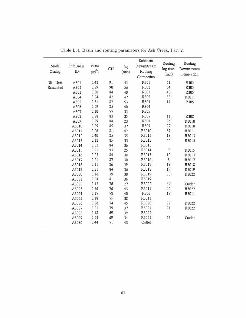
Table B.4: Basin and routing parameters for Ash Creek, Part 2.

61

Table B.5: Basin and routing parameters for South Mesquite Creek, Part 1.

62

Table B.6: Basin and routing parameters for South Mesquite Creek, Part 2.

63

Table B.7: Basin and routing parameters for Calaveras Creek, Part 1.

64

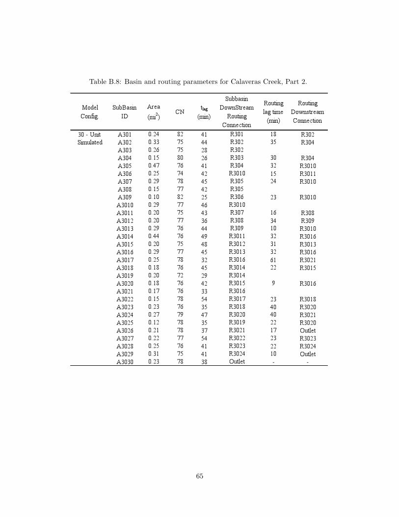
Table B.8: Basin and routing parameters for Calaveras Creek, Part 2.

65

Table B.9: Basin and routing parameters for Pond-Elm Creek, Part 1.

66

Table B.10: Basin and routing parameters for Pond-Elm Creek, Part 2.

67

Table B.11: Summary of runoff volume analysis.

68

Table B.12: Summary of peak discharge analysis.

69

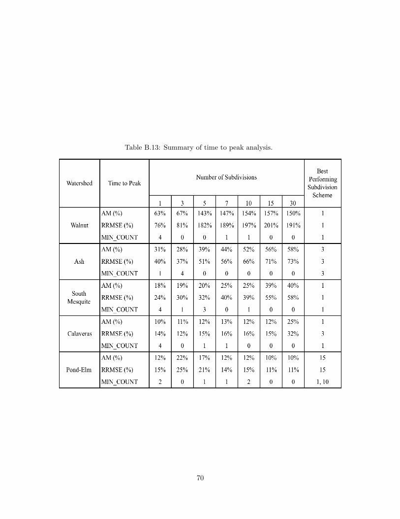
Table B.13: Summary of time to peak analysis.

70

C. Related Documents

Related Documents

The following are abstracts of papers and posters presented at the 2006 Fall American GeophysicalUnion Meeting. None of the posters were directly on the topic of “watershed subdivision,” butthe posters listed had some aspect that the researcher thought had merit in the context of thesubdivision problem. The posters have additional value in presenting a “current-events” snapshotof the broader research questions being addressed by the geosciences community.

For citing these posters the AGU recomends the following citation structure: Author(s) 2006.“Title.” Eos Transactions of American Geophysics Union, Vol. 87, No. 52, Abstract XXXX-XXXX.

H11A-1229

“Understanding Surface water – Ground water Interactions in Arkansas-Red River Basin usingCoupled Modeling”

Joshi, C ([email protected]), Texas A&M University, BAEN, Scoates Hall, TAMU-2117, CollegeStation, Tx 77843, United States

Mohanty, B P ([email protected]), Texas A&M University, BAEN, Scoates Hall, TAMU-2117,College Station, Tx 77843, United States

Subsurface water exists primarily as groundwater and also in small quantity as soil water in theunsaturated zone. This soil water plays a vital role in the hydrologic cycle by supporting plantgrowth, regulating the amount of water lost to evapo-transpiration and affecting the surface water– groundwater interaction to a certain extent. As such, the interaction between surface water andgroundwater is complex and little understood. This study aims at investigating the surface water–groundwater interaction in the Arkansas-Red river basin, using a coupled modeling platform. Forthis purpose, an ecohydrological model (SWAP) has been coupled with the groundwater model(MODFLOW). Inputs to this coupled model are collected from NEXRAD precipitation data at aresolution of 4 km, meteorological forcings from Oklahoma mesonet and NCDC sites, STATSGOsoil property data, LAI (Leaf Area Index) data from MODIS at a resolution of 1 km, and DEM(Digital Elevation Model). For numerical modeling, a spatial resolution of 1 km and a temporalresolution of one day is used. The modeled base flow and total groundwater storage change wouldbe tested using ground water table observation data. The modeled ground water storage is further

71

improved using GRACE (Gravity Recovery and Climate Experiment) satellite data at a resolutionof 400 km, with the help of appropriate data assimilation technique.

TxDOT Researcher’s Comments: Used GIS to parameterize two models. Limited presentation onparameter uncertainty, not sure how applicable to smaller scale models approach has. Appearsthat ET and infiltration are used to adjust match to groundwater storage.

H11A-1230

“Solute Response To Arid-Climate Managed-River Flow During Storm Events”

McLean, B ([email protected]), Arizona State University, School of Earth and Space Exploration,POB 871404, Tempe, AZ 85287, United States

Shock, E ([email protected]), Arizona State University, School of Earth and Space Exploration, POB871404, Tempe, AZ 85287, United States

Storm pulses are widely used in unmanaged, temperate and subtropical river systems to resolve in-stream surface and subsurface flow components. Resulting catchment-scale hydrochemical mixingmodels yield insight into mechanisms of solute transport. Managed systems are far more com-plicated due to the human need for high quality water resources, which drives processes that aresuperimposed on most, if not all, of the unmanaged components. As an example, an increasinglylarge portion of the water supply for the Phoenix metropolitan area is derived from multiple sur-face water sources that are impounded, diverted and otherwise managed upstream from the urbancore that consumes the water and produces anthropogenic impacts. During large storm events thismanaged system is perturbed towards natural behavior as it receives inputs from natural hydro-logic pathways in addition to impervious surfaces and storm water drainage channels. Our goalsin studying managed river systems during this critical transition state are to determine how thewell-characterized behavior of natural systems break down as the system responds then returnsto its managed state. Using storm events as perturbations we can contrast an arid managed sys-tem with the unmanaged system it approaches during the storm event. In the process, we canextract geochemical consequences specifically related to unknown urban components in the form ofchemical fingerprints. The effects of river management on solute behavior were assessed by takingadvantage of several anomalously heavy winter storm events in late 2004 and early 2005 using arigorous sampling routine. Several hundred samples collected between January and October 2005were analyzed for major ion, isotopic, and trace metal concentrations with 78 individual measure-ments for each sample. The data are used to resolve managed watershed processes, mechanisms ofsolute transport and river mixing from anthropogenic inputs. Our results show that concentrationsof major solutes change slowly and are independent of discharge downstream from the dams ontwo major tributaries. This is indicative of reservoir release water. In addition, a third input isderived from the Colorado River via the Central Arizona Project canal system. Cross plots in-cluding concentrations of solutes such as nitrate and sulfate from downstream of the confluenceindicate at least three end-member sources, as do Piper diagrams using major anion and cationdata. Dynamic contributions from natural event water and urban inputs can be resolved from theslowly changing release water, and may dictate the short-term transport of pollutants during thestorm-induced transition state.

72

TxDOT Researcher’s Comments: Used regulatory structures to introduce tracers. Transit timesnot clear in actual presentation. Clever use of tracers and controlled water releases.

H11A-1231

“The role of hillslopes in stream flow response: connectivity, flow path, and transit time”

McGuire, K J ([email protected]), Plymouth State University & USDA Forest Service,Center for the Environment 17 High Street MSC 63, Plymouth, NH 03264, United States

McDonnell, J J ([email protected]), Oregon State University, Department of ForestEngineering, Corvalls, OR 97331, United States

Subsurface flow from hillslopes is widely recognized as an important contributor to stream flowgeneration; however, processes that control how and when hillslopes connect to streams remainunclear. Much of the difficulty in deciphering hillslope response in the stream is due to riparianzone modulation of these inputs. We investigated stream and hillslope runoff dynamics in a 10ha catchment in the western Cascades of Oregon where the riparian zone has been removed bydebris flows, providing an unambiguous hillslope hydrologic signal to the stream channel. Watertransit time was used as a framework to develop a conceptual stream flow generation model forthe small basin. We based our conceptualization on observations of hydrometric, stable isotope,and applied tracer responses and computed transit times for multiple runoff components using asimple linear systems model. Event water mean transit times (8 to 34 h) and rapid breakthroughfrom applied hillslope tracer additions, demonstrated that contributing areas extend far upslopeduring events. Despite rapid hillslope transport processes during events, vadose zone water andrunoff mean transit times during non-storm conditions were greater than the timescale of stormevents. Vadose zone water mean transit times ranged between 10 and 25 days. Hillslope seepageand catchment baseflow mean transit times were between 1 and 2 years. We describe a conceptualmodel that captures variable physical flow pathways and transit times through changing antecedentwetness conditions that illustrate the different stages of hillslope and stream connectivity.

TxDOT Researcher’s Comments: Used GIS and slopes, soil types, and other characteristics.Grouped characteristics by location to identify subwatersheds. Goal was not same as our researchbut the use of hydrologic response units that are physically connected was clever. Tracer tests areused to test research hypotheses.

H11A-1232

“Linking Rainfall, Soil Water Movement, and Groundwater Dynamics to Runoff in a Steep Hillslope:A Topdown Approach”

McDonnell, J J ([email protected]), Oregon State University, 204 Peavy Hall,Department of Forest Engineering, Corvallis, OR 97331, United States

van Verseveld, W J ([email protected]), Oregon State University, 204 PeavyHall, Department of Forest Engineering, Corvallis, OR 97331, United States

The causal linkages between rainfall patterns, soil water response, development of transient ground-

73

water and resulting subsurface stormflow on steep hillslopes remains poorly understood. Most stud-ies to date have relied on short term (hours to days) datasets to characterize the runoff generationprocess of hillslopes or focused on one part of the system. We link rainfall, soil water movement,and groundwater dynamics for a highly instrumented hillslope at Watershed 10 at the H.J. AndrewsExperimental Forest in Oregon, USA. Our hydrometric data from groundwater wells, tensiometers,soil moisture probes and hillslope runoff from a 10 meter wide trench were collected for a periodof one year beginning in Fall 2004. This dataset enabled us to isolate and identify through datamining techniques how rainfall patterns control soil water movement, groundwater dynamics andsubsurface stormflow under different antecedent wetness conditions. (Un)saturated fluxes, bothvertical and lateral at 30 and 70 cm, calculated from the tensiometers, increased exponentiallywith a linear increase in mean or maximum intensity. The timelag between rainfall intensity andsoil water flux, based on linear regression analysis, decreased with wetter conditions. Transientsaturation at subtle changes in hydraulic conductivity within the soil profile occurred during thestorm peaks. Groundwater development was very patchy, with maximum heights of about 20 cmabove the bedrock layer. The relationship between groundwater height and hillslope discharge wasnon-linear. Tree regression analysis of hillslope discharge showed that during high flow conditions,antecedent wetness and mean and maximum intensity dominated system behavior. At low flowconditions, antecedent wetness alone appeared to predict hillslope discharge. Applying these datamining techniques improved our understanding of the hierarchy of process controls on hillsloperunoff and uncovered new predictive rules for subsurface flow generation.

TxDOT Researcher’s Comments: Companion to McGuire paper. Focused on the infiltration (lossmodel) signal. Also explicit mention of lag time as a hydrologic variable of interest.

H11A-1234

“The Integrated Landscape Hydrology Model (ILHM), a Fully-Distributed Approach to SimulateRegional Watershed Hydrologic Processes”

Hyndman, D W ([email protected]), Michigan State University, Department of Geological Sci-ences 206 Natural Science Building, East Lansing, MI 48824, United States

Kendall, A D ([email protected]), Michigan State University, Department of Geological Sciences206 Natural Science Building, East Lansing, MI 48824, United States

Modeling fine-scale regional landscape and subsurface hydrology with fully-distributed process mod-els requires data and computational resources that have only recently become available. For thisreason most hydrologic models either do not represent crucial hydrologic processes or are not prac-tical for regional-scale simulations. To overcome these limitations we linked a set of existing codeswith novel approaches in the new Integrated Landscape Hydrology Model (ILHM), designed to in-tegrate widely-available GIS and remotely-sensed data using a simple parameterization The ILHMis a loosely-coupled suite of codes that allows fine-scale numerical modeling for some processes whileintegrating simpler water-balance models at disparate temporal and spatial scales. This approachenables individual process models to be swapped with different modules or with measured data.Currently, the ILHM includes codes that simulate canopy and soil processes, snowpack accumu-lation and melt, surface ponding and runoff, shallow sub-surface flow, and both unsaturated and

74

saturated groundwater flow. The ILHM also has potential as a tool to simulate fluxes through largeungaged basins and evaluate historical and future hydrologic scenarios. We present an applicationof the ILHM to a 137 square kilometer catchment within the larger Muskegon River Watershed innorthern-lower Michigan. A comparison of model outputs to measured and gaged stream dischargesdemonstrates that the ILHM is capable of predicting hydrologic fluxes with reasonable accuracywithout significant parameter calibration. In addition, the model results suggest interesting andimportant linkages between land use and groundwater recharge.

TxDOT Researcher’s Comments: Used GIS and existing computer codes to develop continuoussimulation responses. Performance seems about same as lumped parameter (researcher opinion).Vague presentation on how results were interpreted.

H11A-1242

“Coupling of Hydrological Models to Assess the Impacts of Changes in Surface and SubsurfaceWater Extraction on Stream Flows”

guzha, a C ([email protected]), Utah State University, College of Engineering, Logan, UT 84321,United States

Bulatewicz, T ([email protected]), Kansas State University, Computing and Information Science,Manhattan, KS 66506, United States

Hardy, T ([email protected]), Utah State University, College of Engineering, Logan, UT 84321,United States

Although it is commonly understood that the extraction of groundwater from the natural envi-ronment can have a significant affect on the hydrological processes throughout a watershed, theprecise affect on different processes is not well understood. Existing models are able to accuratelysimulate the effect of extraction on individual systems, but holistic models are needed to study theeffect across different systems. The primary objective of this study is the development, applicationand investigation of a coupled modeling approach, combining two well- known models, the UnitedStates Geological Survey’s Modular Finite-Difference Groundwater Flow Model (MODFLOW) andthe topography based TopModel, in order to simulate complex hydrological processes in a mesoscalewatershed. The models have been coupled through the use of the InCouple model coupling frame-work. Through the use of lightweight model interfaces, prototype couplings between the modelswere quickly created with minimal changes to the model source codes. These couplings, though,were largely simplified (not spatially distributed, one-way interaction only, and used preliminarydata from the Tenmile watershed in Washington State, USA). The water table elevations simu-lated by MODFLOW were used by TopModel in its simulation of runoff. In our current work, weextend this simple coupling such that the spatial distribution of the groundwater is represented inMODFLOW, and the interaction between the models is bidirectional such that TopModel uses thewater table elevations simulated by MODFLOW, and the recharge calculated by TopModel affectsthe water table elevation simulation in MODFLOW. We present the results of this bidirectionalinteraction between the models as applied to our study site. Our long term goal is to use therapid prototyping capability of the InCouple framework to couple other models to MODFLOW

75

to develop holistic models that can be used to study the effects of groundwater extraction at themesoscale watershed level.

TxDOT Researcher’s Comments: Integrated MODFLOW and TOPMODEL for large-scale water-shed simulations. Appears to be continuous simulation. Limited performance results (none) werepresented in the poster. No attempt to lump – all watersheds are discritized to the DEM resolution.

H13A-1349

“Linking the topography signature of LIDAR-derived vegetation types and geomorphic processesas preliminary steps in integrating landscape evolution with vegetation dynamics”

Tarolli, P ([email protected]), Department of Land and Agroforest Environments, Universityof Padova, viale dell Universitiy – 16, Legnaro, PD 35020 Italy

Istanbulluoglu, E ([email protected]), Departments of Geosciences and Biological Systems Engineer-ing, University of Nebraska-Lincoln, 200 Bessey Hall, Lincoln, NE 68588, United States

Dalla Fontana, G ([email protected]), Department of Land and Agroforest Environ-ments, University of Padova, viale dell’Universit? 16, Legnaro, PD 35020 Italy

In the Italian Alps, dominated by a high altitude climate and characterized by extreme slopemovement processes, topography plays a key role in the redistribution of vegetation over the land-scape. There is significant evidence that vegetation distribution on the Alpine basins influencesthe frequency and magnitude of sediment yields. In this study we investigate the links betweentopography and vegetation species in a small Alpine catchment with an elevation range of 1500to 2000 m a.s.l., with cold snowy winters, and wet summers, in order to decipher the influenceof biota on geomorphic processes in atypical high-latitude Alpine headwater setting. In the studyarea vegetation is mostly represented by grass species (high altitude grassland), but also shrubs(Alnus viridis), and high tree forest (Picea abies) are common. We evaluate the distribution ofvegetation canopies using LIDAR- derived vegetation data. We analyzed the vertical elevationof different vegetation canopy surface layers, and we derived the spatial variation of vegetationspecies following their heights as surveyed in the field. Then we use a high resolution DTM (DigitalTerrain Model), evaluated from filtered bare ground LIDAR points, to derive some mathematicalattributes of landscape morphology including slope gradient, drainage area, aspect, convergenceand topographic wetness index, slope – area diagrams and power-law distribution of areas. Wediscussed the relationships between vegetation species distribution and landform properties.

TxDOT Researcher’s Comments: Note the emphasis on morphology at end of abstract. These re-searchers are attempting to address very similar issue, but focus in on solids (sediment) production.Concepts of slope, area, and slope-area may have value in subdivision research.

H13A-1352

“Upscaling biological quantities in a watershed: combining local predictors with hydro- geomor-phological scaling laws”

Barnes, E A ([email protected]), National Center for Earth-surface Dynamics, St. Anthony Falls

76

Lab, University of Minnesota, 2 Third Avenue SE, Minneapolis, MN 55414, United States

Foufoula-Georgiou, E ([email protected]), National Center for Earth-surface Dynamics, St. AnthonyFalls Lab, University of Minnesota, 2 Third Avenue SE, Minneapolis, MN 55414, United States

Hondzo, M ([email protected]), National Center for Earth-surface Dynamics, St. Anthony FallsLab, University of Minnesota, 2 Third Avenue SE, Minneapolis, MN 55414, United States

Power, M E ([email protected]), Department of Integrative Biology, 4184 Valley Life SciencesBuilding University of California, Berkeley, Berkeley, CA 94720-3140, United States

Recent efforts have demonstrated that local periphyton biomass can be predicted to satisfactoryaccuracy by local physiographic and geomorphic properties in a steep upland stream. For example,periphyton biomass at a point along a river can be predicted by a nonlinear relationship thatinvolves average cross-sectional depth, maximum width, average velocity, exposure to light andnitrate concentration. In this paper, we demonstrate how such local relationships between bioticand abiotic variables can be upscaled to a river reach by using known scaling laws between dischargeand channel properties, known as hydraulic geometry. Using high resolution topography to resolvethe spatial variability of channel quantities, we show that average reach periphyton biomass can beestimated to greater accuracy using upscaling of local geomorphic predictors rather than traditionalaveraging of discrete samples. The implications of this work for sampling design and for interpretingsparse local observations in the context of reach average quantities are also discussed.

TxDOT Researcher’s Comments: Not directly related. Scaling laws to locate where to makemeasurements and to convert averaged and point measurements is worth future study.

H13A-1365

“On the topographic imprint of vegetation: Results from field observations and DEM analysis ofsmall semiarid basins”

Istanbulluoglu, E ([email protected]), University of Nebraska, Department of Geosciences Depart-ment of Biol. Sys. Eng., Lincoln, NE 68588, United States

Vivoni, E R ([email protected]), New Mexico Institute of Mining and Technology, Department ofEarth and Environmental Science, Socorro, NM 87801, United States

Gutierrez-Jurado, H A ([email protected]), New Mexico Institute of Mining and Technology, Depart-ment of Earth and Environmental Science, Socorro, NM 87801, United States

Bras, R R ([email protected]), Massachusetts Institute of Technology, Civil and Environmental En-gineering, Cambridge, MA 02139, United States

Terrestrial landforms result from the complex interactions between biotic and abiotic earth surfaceprocesses forced by climate and tectonics. Understanding the coupled evolution of the physicallandscape system with its biology is a fundamental problem in hydrological sciences. One efficientway to study this coupling is to quantify the differences in vegetation patterns on neighboringhillslopes that are within the same climate, geology and catchment area. Vegetation patterns in

77

the southwestern US are typically organized with respect to the topographic texture with repeatedbands consisting of more mesic plant species in the wetter north-facing slopes, and communitiesdominated by xeric species on the drier south-facing slopes, especially where climate promotesecosystem coexistence. There is evidence that over the long-term such differences in plant specieslead to differential soil and landform development on hillslopes with opposing aspects. In this studywe report preliminary results on the mathematical properties of landscape morphology of varioushillslope aspects in several small-scale (¡10km2) semiarid catchments near Socorro New Mexicobased on field measurements of hillslope profiles and digital elevation model analysis. In the basinsstudied, the north-facing hillslopes are composed of oneseed juniper (Juniperus monosperma) andseveral grass species, have convex hilltops and planar slopes atypical of diffusive landforms. Thesouth-facing slopes are primarily creosote bush (Larrea tridentata), and visually more dissected andconcave than the north facing slopes, displaying geomorphic signatures of fluvial erosion. Alongthe head slopes, often an active ecotone serves as a boundary between the ecosystems. Our resultssuggest that even subtle differences in the vegetation type under essentially the same climate andgeologic controls leave detectable signatures on the mathematical properties of landscape organi-zation and morphology.

TxDOT Researcher’s Comments: More GIS and DEM work – related to biology and solids pro-duction. Paper notes that orientation matters (North slopes are different than South slopes) in thecontext of vegetation type and consequently erosion patterns. Limited practical use for subdivisionproject, but again an area worthy of future consideration.

H13A-1372

“Exploring possible tight inter-connections between climate, soil, topography through constrainingby empirical measure of annual water balance”

Li, H ([email protected]), University of Illinois at Urbana-Champaign, 2521 Hydrosystems Lab, De-partment of Civil and Environmental Engineering, 250 N. Matthews Avenue, Urbana, IL 61801,United States

Sivapalan, M ([email protected]), University of Illinois at Urbana-Champaign, 220 Davenport Hall,607 S. Matthews Avenue, Urbana, IL 61801, United States

Horton overland flow, Dunne overland flow and subsurface flow are the three dominant mechanismscontributing to runoff generation. The Dunne diagram (Dunne, 1978) qualitatively interprets thatthe occurrence and dominance of different mechanisms are significantly affected by climatic condi-tions, soil characteristics and topography. In this work, the climate, soil and topographic controlson annual water balance are examined. A simple distributed hydrologic model has been built forthis purpose, which is comprehensive enough to simulate the effects of different combinations ofclimate, soil and topography, and generate a diversity of runoff generation mechanisms. A small setof dimensionless similarity variables, which are physically meaningful, have been shown to explainthe competition between the wetting, drying, storage and drainage functions of the watershed thatunderlie this model predicted behavior. Each combination of these dimensionless numbers could befeasible in theory, but only some combinations actually occur in nature. By constraining the predic-tions of the model with the empirical Budyko curve, we narrow down to these feasible combinations.

78

At the very least the resulting quantitative climate, soil and topography interconnections could bepotentially tested in the field, and if deemed reasonable, also used to constrain hydrological modelpredictions. The paper will present results from this thought experiment and the ramifications ofthe results for future field studies and hydrological modeling.

TxDOT Researcher’s Comments: Significant work in our context. Researchers have examined lossmodels and highly distributed models, then by non-dimensionalizing have lumped results (uninten-tionally). Little immediate practical value, but suggests current research directions are meaningful.

H13B-1376

“Impacts of climate variability and change on flood frequency: a comparative study of catchmentsin Perth, Newcastle and Darwin, Australia”

Samuel, J ([email protected]), School of Environmental Engineering, University of WesternAustralia, 35 Stirling Highway, Crawley, WA 6009 Australia

Sivapalan, M ([email protected]), Department of Geography University of Illinois at Urbana-Champaign, 220 Davenport Hall, MC-150, 607 S. Mathews Avenue, Urbana, IL 61801, UnitedStates

Struthers, I ([email protected]), School of Environmental Engineering, University of West-ern Australia, 35 Stirling Highway, Crawley, WA 6009 Australia

Traditional flood frequency analysis assumes stationarity, and thus cannot account for non-satationaritycaused by long-term climate variability and change. In this study, we demonstrate that the proba-bility distribution of annual maximum floods is functional upon multi-annual, multi-decadal trendsand climate change in local climate. Three locations in Australia, namely Perth, Newcastle andDarwin are selected and compared to explore the impact of climate variability and change onflood frequency. Analysis is performed using a stochastic rainfall model coupled with a continuousrainfall-runoff model that captures the water balance variability at a multiplicity of time scalesranging from event to seasonal, inter-annual and inter-decadal time scales. Climate variabilityand change are incorporated using different parameterisations of the rainfall model, based uponanalysis of observed rainfall data and selected climate scenarios. We present six climate scenarioslinked between ENSO (El Nino Southern Oscillation) and IPO (Interdecadal Pacific Oscillation)in Newcastle, and six different climate scenarios for Perth and Darwin that are related to ENSOand an apparent shift in climate, identified by statistical analysis, occurring from 1970. The resultsshow that La Nina (ENSO negative) years cause higher annual maximum floods compared to ElNino (ENSO positive) and ENSO neutral years during both IPO (+) and IPO(-) in Newcastleand pre- and post-1970 in Darwin and Perth. The impact of ENSO on annual maximum floodsin Newcastle cacthment is enhanced when the IPO is negative. For Perth, the impact of ENSOweakens post-1970, while it strengthens in Darwin. This research shows that non-stationarity inclimate associated with ENSO and long term climate shifts has a significant impact upon floodfrequency in a variety of Australian climates.

TxDOT Researcher’s Comments: Comparative study of two watersheds was of interest in thisposter. Authors alluded to difficulty in finding otherwise similar watersheds to examine spatial

79

effect of climate on response. Such problem is related to subdivision issue.

H13B-1377

“The Effects of Land use on Soil Properties and Runoff Response at the CATIE Farm, Turrialba,Costa Rica.”

Toohey, R ([email protected]), University of Idaho Environmental Science Program, MorrillHall 216 P.O. Box 443006, Moscow, ID 83844-3006, United States

Toohey, R ([email protected]), Centro Agronomico Tropical de Investigacion y Ensenanza,Apartado Postal 7170 Sede Central, Turrialba, 7150 Costa Rica

Brooks, E S ([email protected]), University of Idaho Department of Biological and AgriculturalEngineering, P.O. Box 440904, Moscow, ID 83844-0904, United States

Jones, J ([email protected]), Centro Agronomico Tropical de Investigacion y Ensenanza, ApartadoPostal 7170 Sede Central, Turrialba, 7150 Costa Rica

Boll, J ([email protected]), University of Idaho Department of Biological and Agricultural Engi-neering, P.O. Box 440904, Moscow, ID 83844-0904, United States

Runoff response in humid tropical areas often is assumed to occur due to infiltration excess. Rainfallintensities in these areas can be monstruous. However, at the Centro Agronomico Tropical deInvestigacion y Ensenanza (CATIE) farm near Turrialba in Costa Rica, we have observed thatvolcanically derived soils have very high infiltration capacities, depending on the land use type,suggesting that saturation excess overland flow mechanism are important in explaining the runoffresponse. In this study we compared field-scale (1-6 ha) runoff response of four different typesof prominent land use on the CATIE farm: forest, a coffee agroforestry system, sugar cane, andpasture. The research site is located at approximately 650 masl in deep soils on the tropical wetCaribbean slope of Costa Rica. Hydrograph analysis of observed runoff data suggest that the runoffmechanism in forest, coffee and sugar cane sites depends much more on the amount of soil storage(e.g. saturated-excess overland flow) than in the pasture site. The pasture site exhibits more ofan infiltration-excess response. In this presentation we present differences in several soil propertiesthat correlate with land use. We simulated measured runoff responses using the Soil MoistureRouting (SMR) model in this high rainfall, deep soil environment because of its ability to simulatesaturation-excess overland flow and lateral flows.

TxDOT Researcher’s Comments: A loss model study, sample sites were located ad-hoc. In our Tx-DOT work we have all used the infiltration-excess (Hortonian) approach as opposed to saturation-excess (Dunne) approach.

H13B-1385

“Evaluating the effect of land use land cover change in a rapidly urbanizing semi-arid watershedon estuarine freshwater inflows”

Sahoo, D ([email protected]), Biological and Agricultural Engineering, 201, Scoates Hall, Texas A

80

and M University, 2117 TAMU, College Station, TX 77843, United States

Smith, P ([email protected]), Biological and Agricultural Engineering, 201, Scoates Hall,Texas A and M University, 2117 TAMU, College Station, TX 77843, United States

Popescu, S ([email protected]), Spatial Sciences Laboratory, 1500 Research Parkway SuiteB223, 2120 TAMU, College Station, TX 77843-2120, United States

Estuarine freshwater inflows along with their associated nutrient and metal delivery are influencedby the land use/land cover (LULC) and water management practices in the contributing watershed.This study evaluates the effect of rapid urbanization in the San Antonio River Watershed onthe amount of freshwater inflow reaching the San Antonio-Guadalupe estuary on the Gulf Coastof Texas. Remotely sensed data from satellite imagery provided a source of reliable data forland use classification and land cover change analysis; while long time series of the geophysicalsignals of stream flow and precipitation provided the data needed to assess change in flow in thewatershed. LULC was determined using LANDSAT (5 TM and 7 ETM) satellite images over 20years (1985-2003). The LANDSAT images were classified using an ENVI. ISODATA classificationscheme. Changes were quantified in terms of the urban expansion that had occurred in past 20years using an urban index. Streamflow was analyzed using 20 years (1985-2004) of average dailydischarge obtained from the USGS gauging station (08188500) closest to the headwaters of theestuary. Baseflow and storm flow were partitioned from total flow using a universally used baseflowseparation technique. Precipitation data was obtained from an NCDC station in the watershed.Preliminary results indicate that the most significant change in land use over the 20 year period wasan increase in the total amount of impervious area in the watershed. This increase in imperviousarea was accompanied by an increase in both total streamflow and in baseflow over the same period.The investigation did not show a significant change in total annual precipitation from 1990 to 2004.This suggests that the increase in streamflow was more influenced by LULC than climate change.One explanation for the increase in baseflow may be an increase in return flows resulting from anincrease in the total number of wastewater treatment plants in the watershed.

TxDOT Researcher’s Comments: Related to our unitgraph work, esp. the developed/undevelopedscoring approach. Limited value in watershed subdivision, but classification of watershed “types”implies subdivision in some sense.

H13B-1386

“Impacts of Land Cover Change on Natural Recharge Levels in the Semi-Arid Edwards AquiferRegion of Texas”

Smith, P K ([email protected]), Texas A&M University, Department of Biological & AgriculturalEngineering 2117 TAMU, College Station, TX 77843-3136, United States

Peschel, J M ([email protected]), Texas A&M University, Zachry Department of Civil Engineering3136 TAMU, College Station, TX 77843-3136, United States

Understanding historical land cover and land use, and other related changes within the hydrologicsignals of a region is advantageous when modeling efforts are considered. However, incorporating

81

different types of land cover changes for hydrologic prediction is not a well-understood task. Froma water resources planning and management perspective, this is of unique interest in semi-aridregions where water availability is often low and thus, water balance sensitivity may be high. Thesemi-arid Edwards Aquifer region of Texas has undergone measurable increases in both populationand impervious surface area over the last twenty years, particularly in the greater metropolitanareas of San Antonio and Austin, the eighth and nineteenth largest cities in the United States,respectively. Consequently, it is expected that the hydrologic response of the Edwards Aquiferhas also undergone changes. The Soil and Water Assessment Tool (SWAT) is a physically- basedmodeling tool for predicting the impacts of land management practices on water, sediment, andagricultural chemical yields. This work presents the results of an algorithm developed to utilizethe SWAT model for estimating natural recharge levels in the semi-arid Edwards Aquifer region ofTexas when land cover and land use, and other related system input changes are considered.

TxDOT Researcher’s Comments: Used SWAT, poster implicitly subdivided by using different landuse classifications. Responses are aggregated at watershed scale – effect of subdivision unable tobe accessed.

H13I-05

“Modeled Response of the low Gradient Portions of the Fly and Strickland Rivers to Post- GlacialSea-Level Rise”

Lauer, J W ([email protected]), Seattle University, Department of Civil & Environmental Engi-neering Seattle University, Seattle, WA 98122-1090, United States

Parker, G ([email protected]), University of Illinois, Department of Civil Engineering and Depart-ment of Geology 2527c Hydrosystems Lab, MC-250 205 N Matthews Avenue, Urbana, IL 61801,United States

Dietrich, W E ([email protected]), Department of Earth and Planetary Science, Univer-sity of California, Berkeley, CA 94720-4767

River valleys evolve in response to upstream boundary conditions such as water and sedimentsupply and to downstream conditions such as sea level. The low gradient sand-bed portion ofthe Fly River System in Papua New Guinea provides a unique opportunity to study the effectof sea level change on a system with significantly different sediment supplies to its two majortributaries. In its present-day state, the larger of the two main tributaries, the Strickland River, issignificantly steeper and less flood prone than the smaller tributary, the middle Fly River (i.e. theFly River above the confluence with the Strickland). The difference is usually ascribed to a morerapid and complete response to sea-level change along the Strickland River than along the middleFly River driven by the significantly larger sediment supply to the Strickland. This hypothesisis tested using a numerical model for river valley evolution over 1000 to 10000 year timescales.The model includes the three main low- gradient sand-bed reaches in the system, the middle Flyand Strickland Rivers (above the confluence) and the Lower Fly River (below the confluence). Themodel is theoretically similar to other diffusion-based numerical models for valley infilling. However,the inclusion of backwater in the theory results in an advective-diffusive form that allows a new

82

delta to automatically form upstream of an abandoned delta once sea level stabilizes. The low-stand longitudinal profile is not well constrained along any of the three low gradient reaches of theFly River system. However, model results confirm that for several different hypothetical low-standprofiles and for sediment loads similar to those observed at present, the middle Fly River would nothave been able to keep up with aggradation along the Lower Fly/Strickland axis of the system. Theresults imply that it is unlikely that the low- stand river channel bed was more than approximately10 m below the present-day channel bed near the confluence, consistent with the few available fieldobservations. This is not necessarily apparent if the evolution of Strickland/Lower Fly axis of thesystem is considered alone without the inclusion of the middle Fly River. The results further implythat at glacial low stand, the Lower Fly River may have passed through a – hard zone – that wassignificantly steeper than the present-day Lower Fly River.

TxDOT Researcher’s Comments: Related to low-slope hydrology. Suggested stream-gradient evo-lution can be explained/predicted by tail-water history.

H13H-01 INVITED

“Doing Hydrology Backwards: Inferring Landscape-Scale Rainfall and Evapotranspiration FromStreamflow Time Series”

Kirchner, J W ([email protected]), Dept. of Earth and Planetary Science, University of Cali-fornia, Berkeley, CA 94720-4767, United States

Catchment hydrology is controlled by processes and material properties that are complex, hetero-geneous on all scales, and poorly characterized by direct measurement. This spatial heterogeneityand process complexity implies that any hydrologic model will necessarily entail substantial sim-plifications and generalizations. The essential question is which simplifications and generalizationsare appropriate for the case at hand. Many ’physically based’ hydrologic models are grounded inan implicit up-scaling premise, which assumes that the small-scale physics in the subsurface will’scale up’ such that the behavior at larger scales (e.g., hillslopes or catchments) will be describedby the same governing equations (e.g., Darcy’s Law, Richards’ equation), with state variables (e.g.,water flux, volumetric water content, hydraulic potential) that are averaged, and with ’effective’parameters that somehow subsume the heterogeneity of the subsurface. There are reasons to be-lieve that this upscaling premise may often be incorrect, and that the effective governing equationsfor these heterogeneous systems may be different in form (not just different in the parameters)from the equations that describe the small- scale physics. Here I describe an approach for deter-mining the constitutive equations that describe catchment behavior at the small-catchment scale.This approach considers the catchment as a first-order nonlinear dynamical system, and estimatesits (nonlinear) governing equations at catchment scale, directly from field data. This approachassumes that discharge depends on the aggregate volume of water stored in the catchment, butmakes no a priori assumption about the functional form of this storage-discharge relationship, in-stead determining it from rainfall-runoff data. This approach not only allows one to predict runofffrom measurements of rainfall, but also allows one to do hydrology backwards: that is, to infereffective rainfall and evapotranspiration at whole-catchment scale, directly from runoff time-seriesdata. This approach can potentially be used to ground-truth remote sensing estimates of rainfalland evapotranspiration time series.

83

TxDOT Researcher’s Comments: Related to all our work. While not specifically on subdivision, theauthor’s implication that doing hydrology backwards is a strong argument for our team’s pursuitof the ad-hoc division research method as well as ensuring that any subdivision scheme aggregrateand dis-aggregate without impacting the lumped response signal.

84

Subdivision of Texas Watersheds for H

ydrologic Modeling

Report No. 0-5822-01-2

Texas Tech University | Lubbock, Texas 79409P 806.742.3503 | F 806.742.4168


David B. Thompson and Theodore G. Cleveland

Performed in Cooperation with the Texas Department of Transportation and the Federal Highway Administration

Research Project 0-5822 Research Report 0-5822-01-2 http://www.techmrt.ttu.edu/reports.php