suborna shekhor ahmed department of forest resources management faculty of forestry, ubc western...
TRANSCRIPT

Suborna Shekhor Ahmed
Department of Forest Resources Management Faculty of Forestry, UBC
Western Mensurationists ConferenceMissoula, MT
June 20 to 22, 2010
Modeling Tree Mortality for Large Regions Using Combined Estimators and
Meta-Analysis Approaches

Objectives
[email protected] Modelling Tree Mortality Using Meta Modelling Slide-2
Develop mortality models for four target species of the Boreal Forest of Canada (aspen, white spruce, black spruce and jack pine)
Data from Alberta, Ontario and Quebec will be used, along with a combined estimator and local mortality models.
To select a combined estimator, several estimators will be proposed and tested using the PSP data from Alberta.
For this presentation, I will present preliminary results of testing combined estimators using PSP data from Alberta for aspen.

Tree Mortality
[email protected] Modelling Tree Mortality Using Meta Modelling Slide-3
Tree mortality is an important aspect of stand dynamics and is commonly expressed in terms of loss of volume or basal area per year.
Cause and time of death are very important to model the tree mortality. The following variables are considered for modeling tree mortality:
Diameter at breast height (DBH), Annual diameter increment during the preceding interval (DIN), Total basal area per hectare at the beginning of the growth interval (BAHA), Site productivity index, Species composition, Length of the growth interval (L),Other measures of competition.

Generalized Logistic Model
[email protected] Modelling Tree Mortality Using Meta Modelling Slide-4
For repeated measures where the time interval, L, is irregular, a generalized logistic model has been used to model survival
where is the annual probability of survival. s are the unknown parameters with explanatory variables.
sp '
From this, the annual probability of mortality is:
sm pp 1
)( 110 kk xxFx
L
s Fxp
)exp(1
1

Published Mortality (or Survival) Models for Aspen
[email protected] Modelling Tree Mortality Using Meta Modelling Slide-5
ReferenceStudy
location Model
Yao et al. (2001)
Alberta mixed wood forests
Lacerte et al. (2006)
Ontario
Senecal et al. (2004)
Quebec’s boreal forest
)022964.0097591.0696387.0
490443.7001175.098991.0716708.1(
)exp(1
1
2
2
BAHA
DBH
BAHA
SPISC
DINDBHDBHFx
Fxp
SW
L
s
)6.2857.119
00952.0(
)exp(1
1
2
1
DINBAL
DBHFx
Fxps
)5603.17566.02052.0(
)exp(1
11
growthPositionCanopyFx
Fxpm
: white spruce (Picea glauca) species composition as a percentage of BAHA;
SPI: site productivity index; canopy position: an ordinal variable of position of the
tree within the canopy;
growth: corresponds to the last year of radial growth (millimetres);
All other variables are previously defined.
swSC

Meta Modelling Approaches
[email protected] Modelling Tree Mortality Using Meta Modelling Slide-6
Combined Estimator
Meta-modeling approaches use observational data to obtain weights for combining existing local scale models may result in improved precision over the naïve approaches. The general approach would be:
jk
r
jjkcombinedk w ˆˆ
1
: kth estimated parameter using the combination of parameter estimates from the r local spatial models;
: kth estimated parameter for local scale model j;
: weight between 0 and 1 applied to the kth estimated parameters for local scale model j;r : number of local scale models.Sum of the over all regions is 1 for each parameter.
combinedk̂Where,
jk̂
jkw
jkw

Meta Modelling Approaches
[email protected] Modelling Tree Mortality Using Meta Modelling Slide-7
Native Approach 1:
One of the native approaches is to use all available data to fit
a large scale model
Native Approach 2 ( Equal Weights ) :
Giving equal weight to each estimate:
Where,
rw jk /1
: weight between 0 and 1 applied to the estimated parameters for local scale model j; r : number of local scale models.
jkw

Meta Modelling Approaches
[email protected] Modelling Tree Mortality Using Meta Modelling Slide-8
Based on Cochran (Inverse Variances):
Weight the parameters by the inverse of their variances, based on Cochran (1977) and extending to r >2:
where indicates variance of a particular parameter estimate.
r
jjk
jkjkw
1
)ˆvar(/1
)ˆvar(/1
)ˆvar( jk

Meta Modelling Approaches
[email protected] Modelling Tree Mortality Using Meta Modelling Slide-9
Maximum Likelihood
Optimal weights are found that meet a maximum
likelihood objective function.
Options include having the same weights for all parameters versus having differential weights by parameter.
Meta Modelling Approaches
[email protected] Modelling Tree Mortality Using Meta Modelling Slide-10
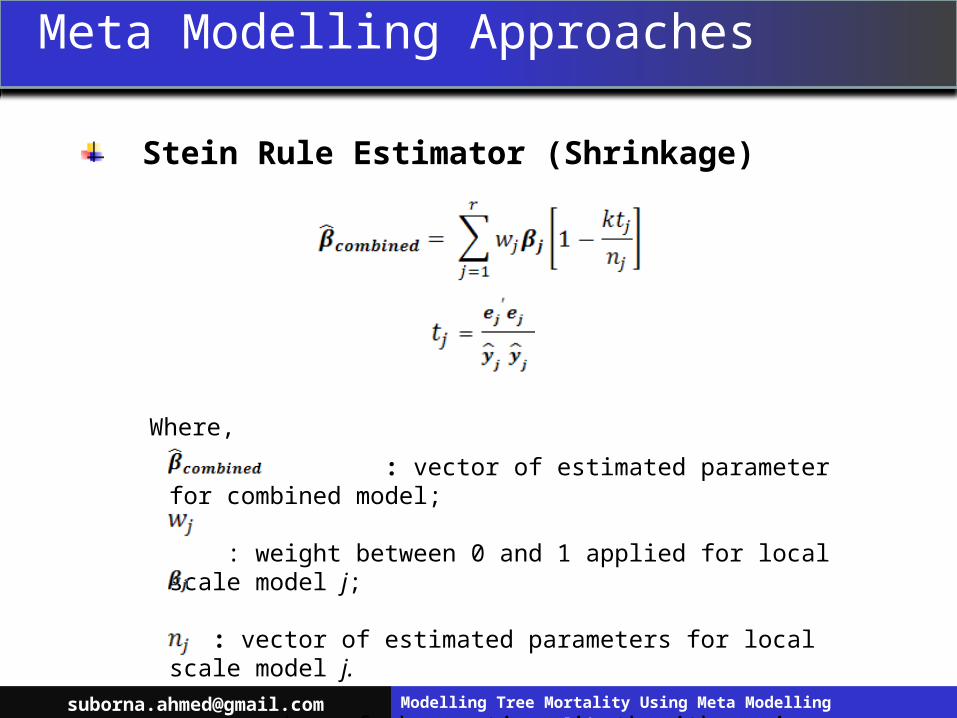
Stein Rule Estimator (Shrinkage)
Where,
: vector of estimated parameter for combined model; : weight between 0 and 1 applied for local scale model j;
: vector of estimated parameters for local scale model j.
: number of observations in the jth region.

Alberta Data
Study includes over 1,700 plots measured up to seven times with a variable number of years between measurements, dispersed over the forested land of Alberta.
Each plot summarized at each measurement period to obtain explanatory variables for modeling for each species and all species combined.
The tree-level variables were then merged with the plot-level variables.
The summarized data were considered as census data at the large spatial scale for this research.
Competition mortality of trees was taken into account.
Plots that have a majority of aspen trees (greater than 30% by basal area per ha in any measurement period) were selected for use.
[email protected] Modelling Tree Mortality Using Meta Modelling Slide-11
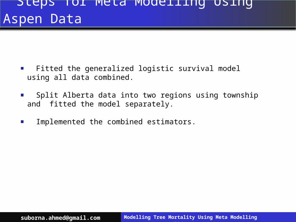
Steps for Meta Modelling Using Aspen Data
[email protected] Modelling Tree Mortality Using Meta Modelling Slide-12
Fitted the generalized logistic survival model using all data combined.
Split Alberta data into two regions using township and fitted the model separately.
Implemented the combined estimators.

Natural Regions of Alberta
Map source: http://www.royalalbertamuseum.ca/vexhibit/eggs/vexhome/regdesc.htm
[email protected] Modelling Tree Mortality Using Meta Modelling Slide-13

Results: Fitted Model
[email protected] Modelling Tree Mortality Using Meta Modelling Slide-14
The probability of survival model for the entire data set and for each region is:
)(
)exp(1
1
43210 SpOtherBALDINDBHFx
Fxp
L
s
Where,
: probability of survival to the end of the period.
DIN: annual diameter increment during the preceding interval.
BAL: basal area of all trees larger than the subject tree.
L: length of the growth interval.
SpOther: percentage of basal area per ha of all trees that were not aspen.
sp

Results: Statistics for Tree- and Plot-Level Variables
[email protected] Modelling Tree Mortality Using Meta Modelling Slide-15
Data set Number
of Plots
Number
of trees
Variable Mean Minimum Maximum
All data
combined269 20835
DBH 23.84 9.2 75.40
DIN 0.17 -0.50 2.28
L 9.25 3.0 30.0
Region 1 220 17611
DBH 24.43 9.2 75.40
DIN 0.17 -0.50 2.28
L 9.24 3.0 30.0
Region 2 49 3224
DBH 20.27 9.2 53.9
DIN 0.16 -0.47 1.06
L 9.41 3.0 19.0

Results: Statistics for Tree- and Plot-Level Variables
[email protected] Modelling Tree Mortality Using Meta Modelling Slide-16
Data set Number
of Plots
Number
of trees
Variable Mean Minimum Maximum
All data
combined269 20835
DBH 23.84 9.2 75.40
DIN 0.17 -0.50 2.28
L 9.25 3.0 30.0
Region 1 220 17611
DBH 24.43 9.2 75.40
DIN 0.17 -0.50 2.28
L 9.24 3.0 30.0
Region 2 49 3224
DBH 20.27 9.2 53.9
DIN 0.16 -0.47 1.06
L 9.41 3.0 19.0

Results: Statistics for Tree- and Plot-Level Variables
[email protected] Modelling Tree Mortality Using Meta Modelling Slide-17
Data set Number
of Plots
Number
of trees
Variable Mean Minimum Maximum
All data
combined269 20835
DBH 23.84 9.2 75.40
DIN 0.17 -0.50 2.28
L 9.25 3.0 30.0
Region 1 220 17611
DBH 24.43 9.2 75.40
DIN 0.17 -0.50 2.28
L 9.24 3.0 30.0
Region 2 49 3224
DBH 20.27 9.2 53.9
DIN 0.16 -0.47 1.06
L 9.41 3.0 19.0
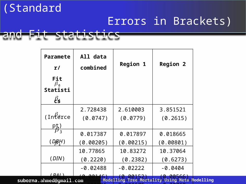
Results: Estimated Parameters (Standard Errors in Brackets) and Fit statistics
[email protected] Modelling Tree Mortality Using Meta Modelling Slide-18
0
1
2
4
Parameter/
Fit
Statistics
All data
combinedRegion 1 Region 2
(Intercept)2.728438 (0.0747)
2.610003 (0.0779)
3.851521 (0.2615)
(DBH)0.017387 (0.00205)
0.017897(0.00215)
0.018665 (0.00801)
(DIN)10.77865 (0.2220)
10.83272 (0.2382)
10.37064 (0.6273)
(BAL)-0.02488 (0.00146)
-0.02222 (0.00152)
-0.0404 (0.00566)
(SpOther)0.002286
(0.000533)0.002675 (0.000614)
-0.00768 (0.00246)
-2logL 11056 9894 1128
3

Results: Estimated Parameters (Standard Errors in Brackets) and Fit statistics
[email protected] Modelling Tree Mortality Using Meta Modelling Slide-19
0
1
2
4
Parameter/
Fit
Statistics
All data
combinedRegion 1 Region 2
(Intercept)2.728438 (0.0747)
2.610003 (0.0779)
3.851521 (0.2615)
(DBH)0.017387 (0.00205)
0.017897(0.00215)
0.018665 (0.00801)
(DIN)10.77865 (0.2220)
10.83272 (0.2382)
10.37064 (0.6273)
(BAL)-0.02488 (0.00146)
-0.02222 (0.00152)
-0.0404 (0.00566)
(SpOther)0.002286
(0.000533)0.002675 (0.000614)
-0.00768 (0.00246)
-2logL 11056 9894 1128
3

Results: Estimated Parameters (Standard Errors in Brackets) and Fit statistics
[email protected] Modelling Tree Mortality Using Meta Modelling Slide-20
0
1
2
4
Parameter/
Fit
Statistics
All data
combinedRegion 1 Region 2
(Intercept)2.728438 (0.0747)
2.610003 (0.0779)
3.851521 (0.2615)
(DBH)0.017387 (0.00205)
0.017897(0.00215)
0.018665 (0.00801)
(DIN)10.77865 (0.2220)
10.83272 (0.2382)
10.37064 (0.6273)
(BAL)-0.02488 (0.00146)
-0.02222 (0.00152)
-0.0404 (0.00566)
(SpOther)0.002286
(0.000533)0.002675 (0.000614)
-0.00768 (0.00246)
-2logL 11056 9894 1128
3

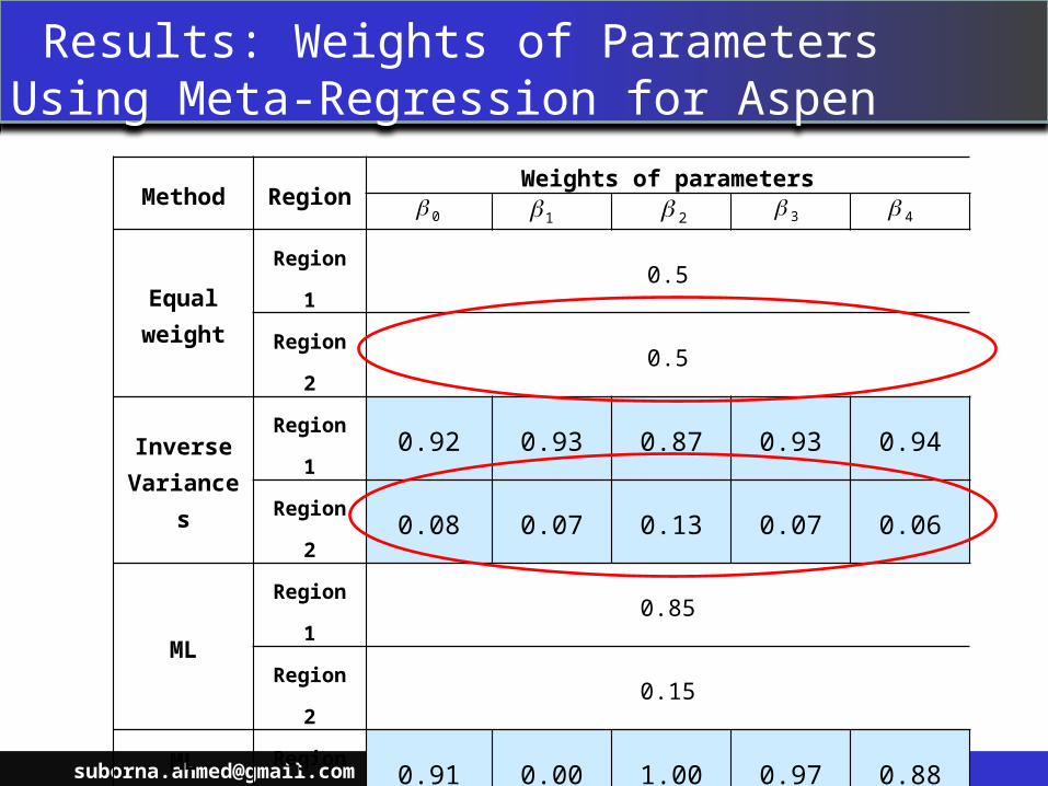
Results: Weights of Parameters Using Meta-Regression for Aspen
[email protected] Modelling Tree Mortality Using Meta Modelling Slide-21
Method RegionWeights of parameters
Equal weight
Region 1 0.5
Region 2 0.5
Inverse Variances
Region 1 0.92 0.93 0.87 0.93 0.94
Region 2 0.08 0.07 0.13 0.07 0.06
MLRegion 1 0.85
Region 2 0.15
ML(Differential
Weight)
Region 1 0.91 0.00 1.00 0.97 0.88
Region 2 0.09 1.00 0.00 0.03 0.12
Stein RuleRegion 1 0.85
Region 2 0.15
0 1 2 3 4
Results: Weights of Parameters Using Meta-Regression for Aspen
[email protected] Modelling Tree Mortality Using Meta Modelling Slide-22
Method RegionWeights of parameters
Equal weight
Region 1 0.5
Region 2 0.5
Inverse Variances
Region 1 0.92 0.93 0.87 0.93 0.94
Region 2 0.08 0.07 0.13 0.07 0.06
MLRegion 1 0.85
Region 2 0.15
ML(Differential
Weight)
Region 1 0.91 0.00 1.00 0.97 0.88
Region 2 0.09 1.00 0.00 0.03 0.12
Stein RuleRegion 1 0.85
Region 2 0.15
0 1 2 3 4

Results: Weights of Parameters Using Meta-Regression for Aspen
[email protected] Modelling Tree Mortality Using Meta Modelling Slide-23
Method RegionWeights of parameters
Equal weight
Region 1 0.5
Region 2 0.5
Inverse Variances
Region 1 0.92 0.93 0.87 0.93 0.94
Region 2 0.08 0.07 0.13 0.07 0.06
MLRegion 1 0.85
Region 2 0.15
ML(Differential
Weight)
Region 1 0.91 0.00 1.00 0.97 0.88
Region 2 0.09 1.00 0.00 0.03 0.12
Stein RuleRegion 1 0.85
Region 2 0.15
0 1 2 3 4

Results: Estimated Parameters Using Meta-Regression for Aspen
[email protected] Modelling Tree Mortality Using Meta Modelling Slide-24
MethodCombined Parameter Estimates
Equal weight
3.2308 0.0183 10.6017 -0.0313 -0.0025
Inverse Variances
2.7112 0.01794 10.7745 -0.0234 0.0021
ML 2.7986 0.018 10.7625 -0.025 0.0011
ML(Differential
Weight)
2.7214 0.0187 10.8327 -0.0228 0.0015
Stein Rule 2.7948 0.018 10.7639 -0.0249 0.0011
0 1 2 3 4

Results: Estimated Parameters Using Meta-Regression for Aspen
[email protected] Modelling Tree Mortality Using Meta Modelling Slide-25
MethodCombined Parameter Estimates
Equal weight
3.2308 0.0183 10.6017 -0.0313 -0.0025
Inverse Variances
2.7112 0.01794 10.7745 -0.0234 0.0021
ML 2.7986 0.018 10.7625 -0.025 0.0011
ML(Differential
Weight)2.7214 0.0187 10.8327 -0.0228 0.0015
Stein Rule 2.7948 0.018 10.7639 -0.0249 0.0011
0 1 2 3 4

Results: Estimated Parameters Using Meta-Regression for Aspen
[email protected] Modelling Tree Mortality Using Meta Modelling Slide-26
MethodCombined Parameter Estimates
Equal weight
3.2308 0.0183 10.6017 -0.0313 -0.0025
Inverse Variances
2.7112 0.01794 10.7745 -0.0234 0.0021
ML 2.7986 0.018 10.7625 -0.025 0.0011
ML(Differential
Weight)
2.7214 0.0187 10.8327 -0.0228 0.0015
Stein Rule 2.7948 0.018 10.7639 -0.0249 0.0011
0 1 2 3 4

Results: Predicted Annual Probability of Survival and Likelihood Using
Meta-Regression and All Data Combined for Aspen
[email protected] Modelling Tree Mortality Using Meta Modelling Slide-27
Method
Predicted
-2logLLive Dead
Mean 25%
(percentile)
75%
(percentile)Mean 25%
(percentile)
75%
(percentile)
Equal weight 0.89 0.86 0.98 0.70 0.55 0.89 11074
Inverse Variances 0.88 0.83 0.98 0.67 0.51 0.86 10996
ML 0.88 0.84 0.98 0.67 0.51 0.87 10994ML
(Differential Weight)
0.88 0.84 0.98 0.68 0.52 0.87 10990
Stein Rule 0.88 0.84 0.98 0.67 0.51 0.87 10994All data
combined 0.88 0.83 0.98 0.66 0.50 0.86 11056
sp

Results: Predicted Annual Probability of Survival and Likelihood Using
Meta-Regression and All Data Combined for Aspen
[email protected] Modelling Tree Mortality Using Meta Modelling Slide-28
Method
Predicted
-2logLLive Dead
Mean 25%
(percentile)
75%
(percentile)Mean 25%
(percentile)
75%
(percentile)
Equal weight 0.89 0.86 0.98 0.70 0.55 0.89 11074
Inverse Variances 0.88 0.83 0.98 0.67 0.51 0.86 10996
ML 0.88 0.84 0.98 0.67 0.51 0.87 10994ML
(Differential Weight)
0.88 0.84 0.98 0.68 0.52 0.87 10990
Stein Rule 0.88 0.84 0.98 0.67 0.51 0.87 10994All data
combined 0.88 0.83 0.98 0.66 0.50 0.86 11056
sp

Results: Predicted Annual Probability of Survival and Likelihood Using
Meta-Regression and All Data Combined for Aspen
[email protected] Modelling Tree Mortality Using Meta Modelling Slide-29
Method
Predicted
-2logLLive Dead
Mean 25%
(percentile)
75%
(percentile)Mean 25%
(percentile)
75%
(percentile)
Equal weight 0.89 0.86 0.98 0.70 0.55 0.89 11074
Inverse Variances 0.88 0.83 0.98 0.67 0.51 0.86 10996
ML 0.88 0.84 0.98 0.67 0.51 0.87 10994ML
(Differential Weight)
0.88 0.84 0.98 0.68 0.52 0.87 10990
Stein Rule 0.88 0.84 0.98 0.67 0.51 0.87 10994All data
combined 0.88 0.83 0.98 0.66 0.50 0.86 11056
sp

Discussion
[email protected] Modelling Tree Mortality Using Meta Modelling Slide-30
The simplest meta-regression approach would be to combine existing models using equal weights which resulted in the highest -2logL.
Maximum likelihood (differential weight ) to find weights resulted in lower -2logL value than other meta-regression approaches.
Conclusion
[email protected] Modelling Tree Mortality Using Meta Modelling Slide-31
Further research will include:
Accuracy testing will be done for the estimators.
One estimator will be selected for use.
Regional models will be fitted for white spruce, black spruce and jack pine using Alberta, Ontario and Quebec PSP data.
Thanks to Alberta, Ontario and Quebec governments for providing PSP data.
Thanks to my committee members:
Dr. Valerie Lemay, UBC.Dr. Steen Magnussen, Nrcan.Dr. Frank Berninger, UQAM.Dr. Peter Marshall, UBC.Dr. Andrew Robinson, U. Melbourne.
Thanks to NSERC and ForValueNet for providing the research funding.
Acknowledgements
[email protected] Modelling Tree Mortality Using Meta Modelling Slide-32
Modeling Tree Mortality for Large Regions Using Combined Estimators and Meta-Analysis
Approaches
[email protected] Modelling Tree Mortality Using Meta Modelling Slide-33