sudan university of science and technology collage of
TRANSCRIPT

Sudan University of Science and Technology
Collage of Engineering
Aeronautical Department
Submitted to the Department of Aeronautical Engineering in partial fulfillment
of the requirements for the degree of Bachelor of Science in Aeronautical
Engineering
Prepared by:
AHMED HAMD-ALNEEL MADNI SULIMAN
AHMED HASSAN AL-NOOR MOHAMMED
ABDULLAHI AL-ALAMEN EHAMER ALI
MOAWIA ALTOM ISMAEL MOHAMMRD
MOHAMMED MAHMOUD OSMAN AHMED
MOSAB MOHAMMED ALI OMER ALMOBARK
Supervised by:
MR.ABD-ALSAMEE
D.INTSAR ABD-ALFTAH
PROF.ALI ALHASEEN
August, 2014

ii

iii
شكزهن.... إن من إن من تعجش انكهمات عن
سانذننا بالإرشاد وانذعاء....!
إن أمهاتنا انعشيشات
إن من بذنىا ننا أسمانهم انغانية و نم يبخهىا عهينا
بانعهم...!
إن معهمينا الأعشاء
إن كم من وقفىا معنا وقذمىا ننا من عهمهم أو
وكانىا دافعا بأ شكم من أشكال الإسناد..
.......!دوماوحافشا نتقذيم الأفضم
نهذي نهم هذا انجهذ انمتىاضع

iv
Dedication
First of all, thanks to ALLAH for all good
things that he had done and giving us
prescience in our Project
This project is dedicated to the country of
our fathers, to the Islam best life religion, to
all the humanity and mankind...............
We as Islamic and Arabic nations we
suffered the terror and injustice of the other
world great nations, but now it is our time
to be strong, now it is our time
To be free ……..

v
بئششاقبث إسبيبث كبج عب صفحت يهئت اطثب قذ
نب رخشا يعب سخق ي يجع الإسشبد انسذاد ف
فب ناء أيبت كشت كثش يبخذإ نشحهت طهت سافع
طلابب اشخكى حبيهب،سبئه الله سبحب أ صعب عهى
شكش ححقق سضا.إنى ي كبا نب سذا يعت عهى
بى طشق انعشفت سخشى نهفعت، أبو يقبهت أضبء الله
إنى كم ي قبسى حم الأيبت فصبس كلاي نجبي يهضو
فبئ، إنى ي حبسى الأيب سفع انقى انعب، إنى
شبحزي انى حشجب انعهى الأسبحزة انشب
د.إنتصار عبد الفتاح
أ.عبد السميع
.علي الحسينبروف
نعد بئر الله ببنجبح إنى انجم اناعذ ا
انخفق، ي كب نى انسبق ببنعطبء
انفبء فأصذقا اناب كهها انعضائى
بطب انخخبو، أخاب يعهب
يخثلا انشكش يصل إنى يشكض أبحبد انطشا
:ف
أ.محمد مهدي بشرى أ.عبد المنعم
انفعبل قبم الأقال انقبم إنى صبحب
ببنال قبم انسؤال
د. صخش بببكش

vi
It is a pleasure to thank those who have contributed to
the realization of this dissertation:
To our families who built us up to face this life.......
To our friends who supported us.........
To our teachers who armed us with knowledgement……
To this great university………..
To the best department ever........
vii
Abstract:
The UAV had been designed in order to meet the
specifications required for surveillance and reconnaissance mission.
It followed the global UAV designs in this industry where the pusher
configuration is dominating over the various other conventional
probabilities. A project was undertaken to study & design Co-axial
propeller for Small unmanned aerial vehicle UAV .the study started
from the comparison between three practical steps ; single propeller ,
single propeller with forward or rearward cascade & Co-axial
propeller. The choice appeared to select a cascade propeller engine to
obtain best criteria with less cost. The design had to be compatible
with the propeller design work being done concurrently. Of
particular interest was comparing the resulting thrust to propel the
UAV at a given airspeed.
The entire propeller design process from airfoil selection to final part
generation in computer-aided drafting program is mentioned. The
Clark-y airfoil defined the propeller cross section.
Design of propeller blades and mechanism to compare the output
thrust between them and determine power that required rotating
propeller. Modification of the mechanism and the manufacture of
propeller from the prototype to the final model will be experimented
and discussed throughout the project.
Static and dynamic analysis for a stability model using the digital
DATCOM had shown UAV is stable statically and dynamically, and
a Simulink model was developed to verify the dynamic modes. A
structural analysis was further initiated to assess the loads acting on
individual components and whether they can sustain the loads or not.

viii
List of Contents:
Dedication ...................................................................................iv
Abstract: ..................................................................................... vii
List of Contents: .......................................................................... viii
Abbreviation: ............................................................................. xiv
List of Tables: .............................................................................. xv
List of Figures: ............................................................................ xvi
List of Symbols: ........................................................................... xxi
2.1PROBLEM STATEMENT: ............................................................. 2
2.1PROPOSED SOLUTION: .............................................................. 3
2.1OBJECTIVES:............................................................................. 3
2.1METHODOLOGY: ...................................................................... 4
2.1Literature Review and Feasibility Study: ...................................... 8
Summary of Design Requirements: ................................................. 9
1.1 Weight of the UAV and its first estimate[2]: ............................. 22
1.1Estimation of the critical performance parameters: ................... 29
1.1Fuselage configuration: ........................................................... 34
1.1Propeller size: ........................................................................ 43
1.1Landing gear & wing placement: .............................................. 47
1.2Better Weight Estimate: .......................................................... 54
Chapter 1 : INTRODUCTION & LITRITUREREVIEW ............... 1
Chapter 2 : CONCEPTUAL DESIGN ................................... 12
Chapter 3 : PRELIMINARY DESIGN ................................... 57

ix
1.2Aerodynamics: ....................................................................... 58
1.2.2Introduction: ....................................................................... 58
1.2.1Aerodynamic coefficients: .................................................... 60
1.2.1Digital DATCOM aerodynamic: .............................................. 69
1.1Performance: ......................................................................... 71
1.1.2Wing loading: ...................................................................... 71
1.1.1Power loading: .................................................................... 72
1.1.1Rate of climb and climb velocity: ........................................... 76
3.2.5 Time to climb: .................................................................... 78
3.2.6 Range: ............................................................................... 79
3.2.7 Endurance: ......................................................................... 80
3.2.8 Landing distance: ................................................................ 80
3.2.9 Take-off distance: ............................................................... 81
3.3 Structural design: .................................................................. 82
3.3.1 V-n diagram: ...................................................................... 82
3.3.2 Gust diagram: ..................................................................... 87
3.3.3 Construction:...................................................................... 90
3.3.4 Fuselage design: ................................................................. 91
3.3.5 Load Determination: ........................................................... 92
3.3.6 Material selection: .............................................................. 97
3.3.7 Stress analysis of fuselage structure: .................................... 101
3.3.8 Sizing of the main members in fuselage structure: ................. 104
1.1 Wing detail design: ............................................................... 105

x
3.3.9 Wing Structure Design: ....................................................... 112
1.1.20 Schrenk’s Curve: .............................................................. 112
3.3.11 Load Estimation on wings .................................................. 117
4.1 Introduction ......................................................................... 130
4.2 Static stability: ...................................................................... 130
4.2.1 Longitudinal Static stability: ................................................ 130
4.2.2 Directional static stability: ................................................... 131
4.2.3 Lateral static stability: ........................................................ 132
4.3 Dynamic stability (Modes of Vibration): .................................. 133
4.3.1 Longitudinal Modes (Steady Modes of Vibration): ................. 133
4.4 Flying Qualities: .................................................................... 138
4.4.1 Longitudinal Flying qualities: ............................................... 139
4.4.2 Lateral Directional flying qualities: ....................................... 141
4.5 Tools to estimate stability derivatives: .................................... 143
5.1 Introduction: ........................................................................ 145
5.2 Definition of coordinate system: ............................................ 145
5.2.2 Body Fixed coordinate Frame: ............................................. 145
5.2.3 Wind and Stability Reference Axis: ....................................... 146
5.3 Rigid Body Equation of Motion: .............................................. 147
5.4 linearization using Small-perturbation theory: ......................... 152
Chapter 4 : STABILITY ANALYSIS ................................... 129
Chapter 5 : MATHMATICAL MODELING OF UAV DYNAMICS
.................................................................................... 144

xi
5.5 Aerodynamic and stability Derivatives .................................... 154
5.5.1Longitudinal Derivatives: ..................................................... 154
5.6 State variable representation of the equations of motion: ........ 158
6.1 Introduction: ........................................................................ 163
6.2 UAV Dynamic Modeling: ........................................................ 163
6.2.1 Nonlinear Model: ............................................................... 163
6.3 Aerodynamic Model: ............................................................. 171
7.1 Theories comparison ............................................................. 175
7.1.1 Momentum theory:............................................................ 175
7.1.2 Blade element theory: ........................................................ 177
7.2 Aerodynamic calculations: ..................................................... 178
7.2.1 Propeller diameter ............................................................. 179
7.2.2 Diameter calculation: ......................................................... 179
7.3 Design envelops: .................................................................. 181
7.3.1 Airfoil selection: ................................................................. 181
7.3.2 Number of Blades, B: .......................................................... 184
7.4 Calculation method and iteration: .......................................... 184
7.5 Cascade design: .................................................................... 192
7.5.1 Stage with downstream guide vanes: ................................... 192
7.6 Co-axial propeller design: ...................................................... 195
Chapter 6 : UAV DYNAMICS MODELING USING SIMULINK
.................................................................................... 162
Chapter 7 : PROPELLER DESIGN .................................... 174

xii
7.7 Practical calculations: ............................................................ 197
Propeller fabrication method: ..................................................... 202
Aerodynamics: ........................................................................... 210
Directional Stability: ................................................................... 216
9.4.2 Three Degree of freedom Lateral model: .............................. 227
Elevator Step ................................................................................................. 240
Aileron Step ............................................................................. 242
Conclusion ................................................................................ 249
References: ............................................................................... 249
APPENDICIES: ............................................................................ 250
APPENDIX A: WING AIRFOIL DATA ............................................... 250
APPENDIX B: CLARK-Y CHARACTRISTICS ........................................ 256
APPEENDIX C: CONISTRAIN DIAGRAM MATLAB CODE .................... 258
APPENDIX D: PERFORMANCE ANALYSIS CODE ............................... 259
APPENDIX E: WING OPTMIZATION ............................................... 262
APPENDIX F: V-N DIAGRAM ......................................................... 264
APPENDIX G: STATE SPACE CALCULATION ..................................... 265
APPENDIX H: MATLAB CODE FOR PROPELLER DESIGN .................... 268
APPENDIX I: PROPELLER BLADE SECTIONS CAD DRAWING ............. 269
APPENDIX J: PROPELLER
PROJECTED VIEWS 270
Chapter 8 : FABRICATION ............................................. 201
Chapter 9 : RESULTS & DISCUSION ................................ 209
Chapter 10 : CONCLUSIONS & RECOMMENDATIONS ...... 249

xiii
APPENDIX K: UAV CAD DRAWING ................................................ 271
APPENDIX L: SNAP SHOT (DATCOM) ............................................. 272
APPENDIX M: SNAP SHOT (AAA) .................................................. 276
APPENDIX N: JAVAFOIL PROGRAM OUUTPUT ................................ 281
APPENDIX O: UAV WEIGHT AND BALANCE .................................... 295

xiv
Abbreviation:
SUAV Small unmanned aerial vehicles
WWII The Second World War
CCRP Co-axial contra rotating propeller
ISTAR intelligence ,surveillance and reconnaissance operations
MAV Micro Air Vehicles
AAA advance aircraft analysis
DATCOM Data compendium
CG Center of Gravity
DCM Direction Cosine Matrix

xv
List of Tables:
Table 1: general aviation constant ............................................. 53
Table 2: better weight estimation ............................................. 55
Table 3: load acting on fuselage ................................................ 93
Table 4: moment about fuselage nose ....................................... 94
Table 5: Material candidates ................................................... 100
Table 6: Stress analysis ........................................................... 102
Table 7: shear flow distribution along fuselage skin ................... 103
Table 8: airfoil selection parameter .......................................... 108
Table 9: load acting in wing ..................................................... 115
Table 10: Aircraft Class ........................................................... 139
Table 11: Long Period Mode damping ratio limits ...................... 140
Table 12: Short period ............................................................ 140
Table 13: Spiral mode- time to double amplitude ...................... 141
Table 14: Roll mode – time constant ........................................ 142
Table 15: Dutch roll damping at frequency requirement ............. 142

xvi
List of Figures:
Figure 1- -2 : Conventional & coaxial propulsion ............................ 2
Figure 1-2: methodology ............................................................ 4
Figure 1-3: Gantt chart ............................................................... 5
Figure 2-1: empty weight fraction ............................................. 23
Figure 2-2: mission profile ........................................................ 25
Figure 2-3: constrain diagram ................................................... 31
Figure 2-4: elliptical nose cone ................................................. 36
Figure 2-5: nose cone drag coefficient ....................................... 37
Figure 2-6: ultra 7000 camera ................................................... 38
Figure 2-7: configuration drag loss ............................................ 39
Figure 2-8: distribution of load along UAV .................................. 41
Figure 2-9: C.G. position ........................................................... 43
Figure 2-10: landing gear configuration ..................................... 47
Figure 2-11 : position of main & nose landing gear ...................... 51
Figure 3-1 : Drag variation graph ............................................... 73
Figure 3-2 : Lift to drag ratios graph .......................................... 74
Figure 3-3 : Power required and available graph ......................... 76
Figure 3-4 : Variation of best rate of climb velocity with altitude
graph ..................................................................................... 77
Figure 3-5 : Rate of climb variation with altitude graph................ 78
Figure 3-6 : Hodograph for climb performance ........................... 79
Figure 3-7: V-n diagram ........................................................... 87
Figure 3-8: shear diagram ........................................................ 94
Figure 3-9: bending diagram ..................................................... 95
Figure 3-10: critical loaded fuselage section ............................... 96
Figure 3-11: fuselage as beam with inertia load .......................... 98
Figure 3-12: minimum mass indicating number ......................... 100
Figure 3-13: performance metric of structure element ............... 101
Figure 3-14: wing layout.......................................................... 105
Figure 3-15: lift distribution for different taper ratio .................. 110
Figure 3-16: lift distribution ..................................................... 111
Figure 3-17: linear lift distribution ............................................ 113
Figure 3-18: elliptical lift distribution ........................................ 115
Figure 3-19: shrenk's load distribution for semi span .................. 116

xvii
Figure 3-20: shrenk's load for the wing ..................................... 117
Figure 3-21: self weight ........................................................... 119
Figure 3-22: shear force diagram for wing ................................. 120
Figure 3-23: bending moment for the wing ............................... 121
Figure 3-24: torque due to normal forces .................................. 122
Figure 3-25: torque due to moment ......................................... 122
Figure 3-26: net torque ........................................................... 123
Figure 3-27: Linear lift distribution .......................................... 124
Figure 3-28: elliptical load distribution ...................................... 124
Figure 3-29: shrenk's for critical condition ................................. 125
Figure 3-30:shear force ........................................................... 126
Figure 3-31: bending moment ................................................. 126
Figure 3-32: torque due to normal force for critical condition ..... 127
Figure 3-33: torque due to moment for critical condition............ 128
Figure 3-34:net torque for critical condition .............................. 128
Figure 4-1 : aircraft response to pitch disturbance ..................... 130
Figure 4-2: Pitching Moment coefficient against angle of attack .. 131
Figure 4-3: aircraft orientation on horizontal plane .................... 131
Figure 4-4:yaw moment coefficients against angle of attack ....... 132
Figure 4-5: rolling moment coefficient against sideslip angle ....... 132
Figure 4-6:phugoid and short period motions ............................ 133
Figure 5-1: Body Fixed coordinate Frame .................................. 146
Figure 5-2:Rigid Body Equation of Motion ................................. 148
Figure 6-1:Three Degree of freedom Longitudinal Model ............ 164
Figure 6-2: aerodynamic block ................................................. 165
Figure 6-3: Lift coefficient block ............................................... 165
Figure 6-4: Drag coefficient block ............................................. 166
Figure 6-5: Moment Coefficient Block ....................................... 166
Figure 6-6: Atmospheric Model ................................................ 167
Figure 6-7: Three Degree of freedom Lateral Model ................... 167
Figure 6-8: Lateral Equation of motion ...................................... 168
Figure 6-9: Aerodynamic Forces and Moments .......................... 169
Figure 6-10:C_y Coefficient Block ............................................. 170
Figure 6-11: Six Degree of freedom Model ................................ 171
Figure 6-12: Atmospheric Model .............................................. 171

xviii
Figure 6-13:Aerodynamic and moment of Six DOF model ........... 172
Figure 6-14: Gravity Model ...................................................... 172
Figure 6-15: Three DOF Linear Longitudinal Model ..................... 173
Figure 6-16: Three DOF Linear Lateral Model............................. 173
Figure 7-1: Momentum theory ................................................ 176
Figure 7-2: propeller blade sections ......................................... 178
Figure 7-3: Clark-y airfoil ........................................................ 183
Figure 7-4: Clark-y lift and drag curve ....................................... 184
Figure 7-5: Blade element theory parameters ........................... 185
Figure 7-6: Axial propeller stage with downstream guide vanes ... 192
Figure 7-7: Axial propeller stage with downstream guide vanes
(velocity triangles for R<1 ) ..................................................... 193
Figure7-8: Cascade arrangement ............................................. 195
Figure 7-9: Flow Model of a Co - Axial Rotor System ................... 196
Figure 7-10: Pitot-tube and the manometer .............................. 198
Figure 8-1: propeller layout ..................................................... 202
Figure 8-2: Propeller curving.................................................... 203
Figure 8-3: carpentry tools ...................................................... 203
Figure 8-4: Propeller wooden model ........................................ 204
Figure 8-5: Propeller casting .................................................... 204
Figure 8-6: Surface finishing .................................................... 205
Figure 8-7: Final product ......................................................... 205
Figure 8-8: System modifications ............................................. 206
Figure 8-9: Cascade blades ...................................................... 207
Figure 8-10: Coaxial system ..................................................... 207
Figure 8-11: Optical digital tachometer ..................................... 208
Figure 8-12: Pitot tube with manometer ................................... 208
Figure 9-1: lift curve slope ....................................................... 210
Figure 9-2: drag against angle of attack .................................... 210
Figure 9-3: Pitching Moment ................................................... 211
Figure 9-4: Roll Moment ......................................................... 211
Figure 9-5: aw Moment .......................................................... 212
Figure 9-6: side force coefficient against beta ............................ 212
Figure 9-7: alpha against Epslon ............................................... 213
Figure 9-8: alpha against d_Epslon ........................................... 213

xix
Figure 9-9: Response to Elevator Impulse ................................. 222
Figure 9-10: angle of attack ..................................................... 222
Figure 9-11: Pitch attitude ....................................................... 223
Figure 9-12: Pitch Rate ............................................................ 223
Figure 9-13: Forward Speed (u) ................................................ 224
Figure 9-14: Upward Speed (w) ................................................ 224
Figure 9-15: Elevator Step of one degree .................................. 225
Figure 9-16: Alpha .................................................................. 225
Figure 9-17: Pitch attitude ....................................................... 226
Figure 9-18: Pitch Rate ............................................................ 226
Figure 9-19: U, W ................................................................... 227
Figure 9-20: Beta .................................................................... 228
Figure 9-21: Phi ...................................................................... 228
Figure 9-22: Psi ...................................................................... 229
Figure 9-23: Roll Rate ............................................................. 229
Figure 9-24: V ........................................................................ 230
Figure 9-25: Yaw Rate ............................................................. 230
Figure 9-26: Beta .................................................................... 231
Figure 9-27: Phi ...................................................................... 231
Figure 9-28: Psi ...................................................................... 232
Figure 9-29: Roll Rate ............................................................. 232
Figure 9-30: Yaw Rate ............................................................. 233
Figure 9-31: Beta .................................................................... 233
Figure 9-32: PHI ..................................................................... 234
Figure 9-33: Psi ...................................................................... 234
Figure 9-34: Roll Rate ............................................................. 235
Figure 9-35: Yaw Rate ............................................................. 235
Figure 9-36: V ........................................................................ 236
Figure 9-37: Alp ..................................................................... 236
Figure 9-38: Euler Angles......................................................... 237
Figure 9-39: p , q , r ................................................................ 237
Figure 9-40: U , V , W .............................................................. 238
Figure 9-41: q ........................................................................ 238
Figure 9-42: Theta .................................................................. 239
Figure 9-43: u ........................................................................ 239

xx
Figure 9-44: w ........................................................................ 240
Figure 9-45: q ........................................................................ 240
Figure 9-46: Theta .................................................................. 241
Figure 9-47: u ........................................................................ 241
Figure 9-48: w ........................................................................ 242
Figure 9-49: Beta .................................................................... 242
Figure 9-50: phi ...................................................................... 243
Figure 9-51: Roll Rate ............................................................. 243
Figure 9-52: Yaw Rate ............................................................. 244
Figure 9-53: Beta .................................................................... 244
Figure 9-54: phi ...................................................................... 245
Figure 9-55: Roll Rate ............................................................. 245
Figure 9-56: Yaw Rate ............................................................. 246
Figure 9-57 ............................................................................ 247

xxi
List of Symbols:
Drag coefficient of blade section
Lift coefficient of blade section
C Blade chord
Propeller RPM
B number of blades
D propeller diameter
P power consumed by propeller
Power coefficient
Q torque
T thrust
Thrust coefficient
Free stream velocity
W local total velocity
Angle of attack
Blade twist
Air density
A propeller disk area
Propeller angular velocity
Velocity at the outlet of the actuator disk

xxii
Pressure at the inlet of the actuator disk
Pressure at the outlet of the actuator disk
Velocity at the outlet of the pipe
Velocity at the inlet of the pipe
Atmosphericpressure at the inlet of the pipe
Area of the inlet of the pipe
Area of the actuator disk
Area of the outlet of the pipe
Propeller radius
Speed of sound
𝑢 𝑟
𝜃
Non-dimensional torque coefficient
Advance ratio

xxiii
The efficiency of the propeller
Aspect Ratio
Wing Span
B Input Matrix
Mean Aerodynamics Chord
Pitching Moment coefficient
Yawing Moment coefficient
Rolling Moment coefficient
Lift coefficient
Drag coefficient
Side force coefficient
, 𝑟𝑜𝑜𝑡 Tip and root chords
Vertical tails lift curve slope
Body axes aerodynamic force in Y directions
Body axes aerodynamic force in x directions
Body axes aerodynamic force in z directions
𝐇 Angular Momentum Vector
, & Angular Momentum x, y, z components
I Inertia tensor
, Moment of inertia about x-axis, y-axis, z-axis
, Products of inertia
Tail arm
Vertical tail arm

xxiv
L Roll moment, Lift Force
N yaw moment
M Pitch moment
Mass
𝐩 Linear momentum
𝑝 Roll Rate
𝑞 Dynamic pressure or pitch Rate
𝑟 Yaw Rate
𝑆 Reference area, Wing plan area
𝑆 Tail area
T Thrust
𝑖 Period
𝑢 𝑢 Velocity in X axes, Control input vector
𝑣 Velocity in Y axis
𝐕 Velocity vector
Airspeed
Horizontal tail volume Ratio
𝑤 Velocity in Z axis‘s
𝔁 State vector

xxv
Greek letters
Angle of attack
Side slip angle (deg)
Aileron deflection
Elevator deflection
Rudder deflection
𝛷, 𝜑 Roll attitude
𝛩, 𝜃 Pitch attitude
Ψ, ψ Yaw attitude
𝜆 Taper Ratio, eigenvalue
𝜂 Tail Efficiency
Air density
Damping ratio

Chapter 1 :
INTRODUCTION &
LITRITUREREVIEW

1
2.1PROBLEM STATEMENT:
Previous UAVs had used conventional propellers which make
UAVs suffer from lack of aerodynamics efficiency, caused by the
trailing slipstream that creates an opposing torque on the fuselage
while rotating. This phenomena has a raised multiple issues such as
the extra drag on fuselage, resulting in a lower thrust & reducing
stability. The thrust –to-weight ratio in co-axial propeller is much
higher than conventional propellers. Other than that, asymmetric
effect on propellers can be avoided.
Conventional propulsion Co-axial propulsion
Figure 1--1: Conventional &
coaxial propulsion

1
2.1PROPOSED SOLUTION:
After extensive research, it's found that the major development can
be implement here is use of cascade scheme or co-axial propeller
rather than conventional one. Recent research shows that the use of
co-axial propeller increase propulsive efficiency as high as
19%.other important advantages is the enhancement of aerodynamic
efficiency.
Design and analysis of cascade & co-axial propeller.
Maximize aerodynamic efficiency by:
1- Wing lets 2- Landing gear fearing
2.4OBJECTIVES:
The project objectives were specified by the project group very early
in the project. These consisted of both primary and extended project
goals
PRIMARY OBJECTIVES:
1. Design UAV with level one flying qualities.
2. Developing dynamic model using SIMULINK.
3. Testing of the three schemes of engine (single propeller, single
propeller with rearward cascade, coaxial propeller).
EXTENDED OBJECTIVES:
1. Encourage continued undergraduate and postgraduate
development of UAVs at the University of Sudan.

1
2. Development of a surveillance system for a UAV which can
stream to a ground based station and allow for autonomous search
and identification of ground based targets.
2.1METHODOLOGY:
Figure 1-2: methodology

1
The Gantt chart:
Figure 1-3: Gantt chart

1
Outlines:
Chapter one includes: introduction, problem statement, proposed
solution, objectives, methodology, literature review and feasibility
study.
Chapter two include: conceptual design, requirements, weight of the
UAV and its first estimate, estimation of the critical performance
parameters, fuselage configuration, propeller size, landing gear &
wing placement, better weight estimate.
aerodynamic analyzed by use digital DATCOM aerodynamic
program. performance analyses by matlab code programs to calculate
wing loading, power loading, rate of climb and climb velocity, time to
climb, rang, endurance, take-off distance, landing distance.
structural design include two designs, fuselage design & wing design
Chapter four include stability analysis: static stability, longitudinal
static stability, directional static stability, lateral static stability,
dynamic stability (modes of vibration), longitudinal modes (steady
modes of vibration), flying qualities, longitudinal flying qualities,
lateral directional flying qualities, tools to estimate stability
derivatives.
Chapter six include UAV dynamics modeling, nonlinear model,
aerodynamic model using Matlab simulink.
Chapter three include preliminary design (aerodynamic ,
performance and structure analysis)
Chapter five include mathmatical modeling of uav
dynamics, it gives an introduction to aircraft modeling.

2
Chapter seven present propeller design, cascade design, stage with
downstream guide vanes, co-axial propeller design, practical
calculations.
Chapter eight shows a fabrication of propeller and the experimental
that done to the propeller.
Chapter nine shows the results & discussion of all project calculations.
Chapter ten shows the conclusions & recommendations

3
2.1Literature Review and Feasibility Study:
The following literature review is a brief summary of the extensive
investigation into Unmanned Aerial Vehicle technology that was
conducted at the beginning of the project. This section has been divided
into literature on aircraft design, propulsion systems.
2.1.2 Statistical Analysis:
A statistical analysis method was utilized by the project group
to design the vehicle. This method was as suggested by both
RAYMER and ROSKAM[2, 3].The statistical analysis method
involves investigating the performance and designs of existing
vehicles and using the information from these designs to construct a
baseline design of the vehicle, which can then be optimized for the
required technical task. The statistics used for this method were those
collected as a result of the market evaluation.
2.1.1 Analyzed UAVs:
A number of commercial UAV platforms were analyzed for their
design parameters. These included UAVS up to and including 100 kg
in takeoff weight, UAVS with both electric internal combustion
systems and with an endurance of at least 2hrs.
AEROSKY:

4
Summary of Design Requirements:
Altitude:
The operational altitude is to be 3km.whiche is a balance
between image clarity and covered area.
Cruise Speed:
As a result from literature cruise speed of 47m/s seems
reasonable. While the main constraint of the cruise speed is
performance of the camera, the cruise speed may be revised after the
design of imaging system and selection of the camera.
Takeoff and Landing:
Is the length of the field required for takeoff and landing For
this aircraft the maximum takeoff field length was 150m, which was
deemed to be short enough to maintain application flexibility and
long enough to reduce power requirements. The landing distance
should be no more than 250m.
Endurance:
The UAV‘s minimum endurance will be 4 hour of continuous
flight in accordance with the maximum mission time from literature
survey result.
Propulsion system:
Contra-rotating propellers have been studied for over 60 years
as a more fuel efficient method of aircraft propulsion. A CRP
consists of 2 sets of propeller blades, one directly behind the other in

20
the axial direction, spinning in opposite directions. Counter-rotating
propellers spin in opposite directions.[4]
The fundamental premise behind CRPs is the elimination of
the tangential velocity, which is considered to be a loss in
performance and efficiency. Contra-rotating propellers can
significantly reduce or even eliminate the tangential velocity of the
propelled air, or swirl losses, and also the torque produced by the
engine. This leads to a more efficient and economical engine and
less torsional loading on the wings. [4]
There has been renewed interest in finding a more
efficient replacement for current Aircraft propulsion systems, with
one such approach utilizing a counter-rotating propeller
Configuration. An initial theory regarding the mechanics of
counter-rotating propellers was developed by Locks in 1941
Since then, many investigations into the advantages of Counter-
rotating propellers have been conducted. For example, Bergmann
and Gray conducted full scale wind tunnel tests on counter-
rotating propellers in both tractor and pusher configurations. It
was found that an 8 to 16% increase in propeller efficiency could be
gained depending upon installation position. In a later test,
Bergmann and Hartman found that the performance of counter-
rotating propellers was significantly improved at lower advance
ratios. McHugh and Pepper have shown that the counter-rotating
propeller configuration is highly receptive to the use of
aerodynamically improved airfoil designs. Other investigations
into the performance of counter-rotating propellers conducted by
Gray have indicated that the overall efficiency o f a counter-

22
rotating propeller is not seriously affected by changes in
rotational speed
Small changes in blade angle of the aft propeller disk. These
changes did, however, have moderate effect when the propeller was
operated at peak efficiency. In an experimental study, Mille found
that the vibration of counter-rotating propellers caused by mutual
blade passage or by blade passage through the wake o f a wing
was not significant. Bartlett has shown that locking or wind
milling one of the propeller components o f a counter-rotating
configuration has a detrimental effect on total propeller
efficiency. For example, a counter rotating propeller with one
propeller disk disabled results in a total propeller efficiency that is
lower than the individual efficiency of the rotating propeller.[5]
The increase in peak efficiency and improved off-design
performance of counter-rotating systems allow for smaller
propulsion units to be installed on the aircraft. The disadvantages
Of counter-rotating propeller configurations include gearbox
Complexity and an increased vibration state caused by the periodic
blade passage. Research conducted by Strake. al. has shown that
with current improvements of present day technology, lightweight
and reliable counter-rotating propeller gearboxes can be built.
Thus, it is evident that counter- rotating propellers can indeed offer a
more efficient means of propulsion.[5]
This brief literature survey has indicated that counter-
rotating propellers exhibit many advantages over single rotation
propellers such as higher peak efficiency, better off- design
performance, and a reduced total torque of the system.[5]

21
Design Development:
The main advantage of counter-rotating propellers stems
from the swirl velocity losses of the front propeller disk being
recovered by the aft propeller disk. The front disk imparts a
tangential velocity to the air as it passes through the front propeller
disk plane. This swirl velocity acts as an additional angular velocity
for the aft disk, without the power plant having to drive the aft disk
at a higher angular velocity. It may be noted that a tangential
interference velocity is recognized by the front disk, but is
typically an order-of-magnitude smaller than other interference
velocities and therefore neglected, resulting in a first-order theory
for the design and analysis of counter-rotating propellers. Airfoil
data , such as lift, drag, and angle of attack are specified for
each radial location along the propeller blade. This is done
through the use of airfoil data banks, utilizing either tabulated
data or empirical formulations that yield airfoil lift and drag as
functions of angle of attack and Mach number.
The airfoil data used in the calculations during the design
process was selected to maximize the lift-to-drag ratio of the
airfoil used at each radial location along the blade. In regions
near the hub, where the propeller blade quickly transitions from an
airfoil to a right circular cylinder, a different approach has been
taken. To accommodate this transition, the chord length is
linearly interpolated from that calculated to a structurally feasible
cylinder at the hub. The design procedure involves calculations,
which include division by the lift coefficient, to determine chord
length. Since the lift coefficient of a circular cylinder is zero, it
may be noted in the development of the theoretical model that it

21
is necessary to maintain a finite- lift coefficient to insure arriving
at positive values of the blade chord. [5]
Co-axial contra rotating propeller (CCRP ) systems promise a
light weight, fuel efficient means for propulsion for the
aerospace industry. The only drawback is its high level
aerodynamic noise.[6]
The research is study about flow around propeller to increase
endurance and thrust by increase the efficiency. The study is
decomposing to tasks that‘s CFD task, experimental task. The study
is a compare between single propeller alone, single propeller with
rearward cascade & dual acting propeller (CO-AXIAL
PROPELLER).

21
Chapter 2 :
CONCEPTUAL DESIGN

11
1.1 Weight of the UAV and its first estimate[2]:
There are various ways to categorize the weight of the UAV.
The following is a common choice:
1- Payload weight Wpayload: the payload is what the UAV intended to
transport (camera & sensors for our case). If the UAV is intended for
military combat use, the payload may include missiles, bombs or
other disposable weapons.
2- Fuel weight Wfuel: this is the weight of the fuel in the fuel tanks.
Since fuel is consumed during the course of the flight, Wfuel is
variable, decreasing with time during the flight.
3- Empty weight Wempty: this is the weight of every else ( the structure,
engines with all accessory equipment, electronic equipment, landing
gears, fixed equipment and anything else that is not payload or fuel ).
The sum of these weights is the total weight of the UAV (Wtotal).
Again Wtotal is varying throughout the flight because fuel is being
consumed. The design take-off weight is the gross weight of the
UAV at the instance it begins its mission. It includes the weight of
all the fuel on board at the beginning of the flight. Hence:
............................................................. (2-1)
: is the fuel weight at the beginning of the flight.
: is the first estimate of the total weight of the UAV. To make this
estimate, equation (2-1) must be rearranged as follows:
............................................................. (2-2)

11
............................................. (2-3)
Solving equation (2-3) for
........................................................................... (2-4)
Although at this stage, we do not have a value of , we can fairly
readily obtain values of ratios of
and
as it can see next. Then
equation (2-4) provides a relation from which can be obtained in
an iterative fashion.
Estimation of the value
:
A new design is usually an evolutionary change of an existing
design. For this reason, historical, statistical data on previous UAVs
provide a starting point for the conceptual design of new UAV. In
particular, fig () is a plot of
versus for a number of similar
UAVs.
Figure 2-1: empty weight fraction
0
0.1
0.2
0.3
0.4
0.5
0.6
0.7
0.8
0.9
0 200 400 600 800 1000 1200 1400
w0

11
That's to say,
Estimation of
:
The amount of fuel required to carry out the mission depends
critically on the efficiency of the propulsive device (the engine
specific fuel consumption & the efficiency of the propellers). It also
depends critically on the aerodynamic efficiency (the lift to drag
ratio). These factors are the principal player-s at the Brequet range
equation given below:
.............................................................................. (2-5)
The total fuel consumed during the mission is that consumed
from the moment the engine is turned on to the moment they are shut
down at the end of the flight. Between these times, the flight of the
UAV can be described by a mission profile, a conceptual sketch of
altitude versus time such as the one shown in fig(2-2). As stated in
the specifications, the mission of our UAV is that of a recognizance
& surveillance type, because of that the mission profile for a simple
cruise with loitering at the required location had been selected. It
starts at the point labeled 0 when the engine is turned on. The take-
off segment is denoted by the segment 0-1, which includes taxing &
take-off. Segment 1-2 denotes the climb to cruise altitude (the use of
straight line here is only schematic & is not meant to imply a
constant rate of climb to altitude). Segment 2-3 & segment 4-5
denote the cruise condition with loiter time at segment 3-4 to fulfill
the mission requirements. Segment 5-6 denotes descent. Segment 6-7
represents landing. The mission profile is shown below:

11
Figure 1-2: mission profile
Each segment of the mission is associated with a weight
fraction, defined as the UAV weight at the end of the segment
divided by the weight at the beginning of the segment. Hence, the
first thing for calculating
is to define the weight fractions of the
mission.
Historical data show that weight fractions of take-off, climb, descent
& landing respectively as follow:
For segments 2-3 & 4-5, Brequet range equation had been
used. This requires the estimate of
. At this stage of design, we
cannot carryout a detailed aerodynamic analysis to predict
, we have
not even laid out the shape of the UAV yet. Therefore, we can only
make a crude approximation based on the data from the previous
UAVs. Hence, a reasonable first approximation for our UAV:

11
Also, we need in the range equation the specific fuel
consumption c & the propeller efficiency η. A typical value of
specific fuel consumption for current UAV reciprocating engines is
0.52 lb of fuel consumed per horsepower per hour:
A reasonable value for the propeller efficiency η for coaxial
propellers engine is 0.8:
From Brequet equation, the ratio
is replaced for the mission
segment 2-3 by
. Hence, eq become:
.............................................................................. (2-6)
⁄
⁄
................................................................................. (2-7)

12
For cruise,
3-4 is a loiter flight where:
Endurance=2h;
= 115.65ft/sec (assumed roughly as (0.75). Based on
competitor study)
Propeller Efficiency (𝜂 )=0.7 (a lower efficiency compared to cruise
is used)
( )=
(same as the cruise SFC)
( ) (
)
⁄
Collecting the various segment weight fractions & getting the
product of them to obtain the ratio of the weight at the end of the
mission to the initial gross weight:
The change in weight is due to the consumption of fuel. If at the end
of the flight, the fuel tanks were completely empty, then:
................................................................................. (2-8)
However, at the end of the mission, fuel tanks are not
completely empty by design. There should be some fuel left in

13
reserve at the end of the mission in case weather conditions or spend
a longer than normal time in loiter condition. Also, the geometric
design of the fuel tanks & fuel system leads to some trapped fuel that
is unavailable at the end of the flight. Typically, 6% allowance is
made for reserve and trapped fuel. Modifying previous equation for
this allowance, we have:
(
)
(
) ( ) =0.07022
Calculation of :
We obtain the values of the ratios
&
which are required
to obtain the initial design take-off weight . Since our UAV is for
recognizance & surveillance, the payload here is a camera in order to
survey a prescribed location. The total weight of the payload is 33.1
lbs. inserting the values above into the equation of :
This is our first estimate of the gross weight of the UAV.
Finally, the weight of the fuel in tanks is calculated. This will
become important later in sizing the fuel tanks.
0.07022

14
Hence:
1.1Estimation of the critical performance parameters:
Estimation for the critical performance parameters[2] is
needed to determine such aspects as maximum speed, range, ceiling,
rate of climb, stalling speed, landing distance & take-off distance.
These parameters namely are( ) , ⁄ , 𝑆⁄ and ⁄ .
Constrain diagram:
The wing loading and power loading are calculated depending upon
design requirements[7]. These requirements are as follows:
Stall speed:
The minimum speed that an aircraft can fly
(
𝑆)
𝑆
Maximum speed:
The power loading ( ) is a non-linear function of the wing
loading ( 𝑆) in terms of maximum speed, and may be simplified
as:

10
(𝑤
𝑝)
𝜂
(
)
(
)
,
&
Take-off distance:
The take-off distance is in the variation of W/Pas a function of W/S
based on STO for a prop-driven aircraft can be sketched using
Equation ()
(
)
𝑥𝑝 ( 𝑆
⁄)
(
) * 𝑥𝑝 ( 𝑆
⁄)+
𝜂
The above equations use to contract the constrain diagram shown in
appendix

12
Figure 1-3: constrain diagram
Configuration layout:
There are some basic configuration decisions to make up front.
Do we use one or two engines? Do we use a tractor (propeller in
front) or a pusher (propeller in back) arrangement (or both)? Will the
wing position be low-wing, mid-wing, or high-wing? Indeed, do we
have two wings, i.e., a biplane configuration?
First, let us consider the number of engines. The weight of
103.57 lb puts our UAV somewhat on the borderline of single- and
twin-engine UAVs. Since the common is to adapt a single engine
from the existing UAVs designs, thus a single one is adequate. We
need 16.5 hp from the constraint diagram of the statistical data can
we get that from a single, existing piston engine. (We have to deal
with an existing engine; rarely is enough incentive for the small
engine manufacturers to go to the time and expense of designing a
new engine.) Examining the available piston engines at the time of
writing, we find that the DA-150is rated at 16.4 hp. This appears to
be the engine for us. It is only 1 hp.more than our calculations show

11
is required based on the rate-of-climb specification. We could tweak
the airplane design, say, by slightly increasing the weight or slightly
decreasing the aspect ratio, both of which would increase the power
required for climb and would allow us to meet the performance
specification with this engine. The free-stream density ratio between
3km and sea level is . Hence, the engine
power at 3km will be ( 𝑝)( ) 𝑝. This is more
than enough to meet the calculated requirement of 15.4 hp for
at3km. Therefore, we choose a single-engine
configuration, using the following engine with the following
characteristics:
DA-150 piston engine:-
Rated power output at sea level: 16.4H0p
Length: 0.637ft
Dry weight: 7.96Ib(3.61 kilos)
Diameter of the base: 122mm
E.C.D: 98mm
Bore: 1.9291 in (49 mm)
Stroke: 1.5748 in (40 mm)
RPM Range: 1,000 to 8,500
RPM Max: 11,000
Fuel Consumption: 3.3 oz/min @ 6,000 RPM
Warranty: Three year

11
Question: Do we adopt a tractor or a pusher configuration?
Some of the advantages and disadvantages of these configurations
are itemized below:
Tractor Configuration Advantages:-
1. The heavy engine is at the front, which helps to move the center
of gravity forward and therefore allows a smaller tail for stability
considerations.
2. The propeller is working in an undisturbed free stream.
3. There is a more effective flow of cooling air for the engine.
Disadvantages:
1. The propeller slipstream disturbs the quality of the airflow over
the fuselage and wing root.
2. The increased velocity and flow turbulence over the fuselage due
to the propeller slipstream increase the local skin friction on the
fuselage.
Pusher Configuration Advantages:-
1. Higher-quality (clean) airflow prevails over the wing and
fuselage.
2. The inflow to the rear propeller induces a favorable pressure
gradient at the rear of the fuselage, allowing the fuselage to close
at a steeper angle without flow separation. This in turn allows a
shorter fuselage, hence smaller wetted surface area.
3. Engine noise in the cabin area is reduced.
Disadvantages:
1. The heavy engine is at the back, which shifts the centre of
gravity rearward,hence reducing longitudinal stability.

11
2. Propeller is more likely to be damaged by flying debris at
landing.
3. Engine cooling problems are more severe.
1.4Fuselage configuration:
Once the take-off gross weight has been estimated, the
fuselage, wing, and tails can be sized. Many methods exist to
initially estimate the required fuselage size. Fuselage length is
empirically related to the gross weight by Equation (2-9) given by
Raymer where for a home-built aircraft:
................................................................................ (2-9)
, that gives
However, the empirical formula above is valid for UAV with
conventional tail. In our case, as the UAV tail has a boom for
connection, the tail is not considered in the fuselage length. Taking
the value above as the total length of the UAV, a factor of 0.55 is
used for fuselage to total length fraction, suggested by Raymer for
pusher configuration keeping the fuselage slightly longer than the
half length of the UAV as is common along the competitor UAVs.
Then the fuselage length becomes:
The height and width of the fuselage are also initially guessed.
The design of the fuselage is based on payload requirements,
aerodynamics, and structures. The overall dimensions of the fuselage
affect the drag through several factors. Hemida, Hassan and
Krajnovic, Siniša (2010)Stated that fuselages with smaller fineness
ratios have less wetted area to enclose a given volume, but more
wetted area when the diameter and length of the cabin are fixed.

11
The higher Reynolds number and increased tail length
generally lead to improved aerodynamics for long, thin fuselages, at
the expense of structural weight. Selection of the best layout requires
a detailed study of these trade-offs, but to start the design process,
something must be chosen. This is generally done by selecting a
value not too different from existing aircraft with similar
requirements, for which such a detailed study has presumably been
done. In the absence of such guidance, one selects an initial layout
that satisfies the payload requirements.
In this UAV fuselage design, the payload requires a fuselage
being able to hold a camera, batteries, servo, and targeting ball.
Except the payload requirement, other considerations are:
1. Low aerodynamic drag
2. Minimum aerodynamic instability
3. ease of assembly and disassembly of fuselage
4. Structural support for wing and tail forces acting in flight,
which involves simple stress analysis for the entire fuselage
.
UAV Shape and Aerodynamics of Fuselage:
UAV Nose and Tail Cone Design:
The fuselage shape must be such that separation is avoided
when possible. This requires that the nose and tail cone fineness
ratios be sufficiently large so that excessive flow accelerations are
avoided.
The aircraft fineness ratios are defined as length divided by diameter,
which including nose fineness ratios and tail cone fineness ratios.
In all of the following nose cone shape equations, L is the
overall length of the nose cone and R is the radius of the base of the

11
nose cone. yis the radius at any point x, as x varies from 0, at the tip
of the nose cone, to L. The equations define the 2-dimensional
profile of the nose shape. The full body of revolution of the nose
cone is formed by rotating the profile around the centerline (C/L).
Note that the equations describe the 'perfect' shape; practical nose
cones are often blunted or truncated for manufacturing or
aerodynamic reasons.
Figure 1-4: elliptical nose cone
There are several shapes available: 3/4 Power, Cone, 1/2 Power,
Tangent give, parabolic, ellipsoid, etc.
Liu Tang-Hong, Tian Hong-qi and Wang Cheng-Yao (2006)
wrote in journal ―Aerodynamic performance comparison of several
kind of nose shapes‖ that as speed of the plane increases, the drag
coefficient increase as well. Different type of fuselage shape can give
different drag coefficient as well. But as shown above, below Mach
number 0.5, the shape of the airplane does not give too much
difference.

12
Figure 1-5: nose cone drag coefficient
In this UAV design, one of key factors in UAV fuselage shape
design is the payload. According to the payloads weights, centre of
gravity as well as the attribution of the different parts, the width,
namely the aircraft lateral diameter is no less than 0.83571.In order
to make sure the Centre of Gravity is behind the aerodynamic centre,
which is design to make sure of the aircraft stability and easily
maneuverability, and based on the fact that the tail of the plane is
relatively high, the batteries and camera should be put into the very
front to counter the weight. As such, the nose should be designed so
as to have enough space to hold the payloads at the very front. That‘s
the main reason of this design.

13
Payload sizing:
The payload here is EO/IR standard .It was selected the ultra
7000 camera setup, with forward and sideways looking camera
options and varying lenses. The pixel pitch of the camera is
approximately 3-5µm.Power required to operate the camera is
28VDC, 450 Watts. The speed needed to focus on objects of interest
will not be an issue with this gimbals‘, which has 2-Axis, 3 Fiber-
Optic gyros Stabilization. The diameter of the camera is about 9
inches; with height 15.2inches.it weighs about 26 lbs. Total system
weight less than 40 lbs.
Figure 1-6: ultra 7000 camera
Except the shape of the fuselage, the nose and tail cone fineness ratio
play an important role in fuselage design as well. Below is a
simulation graph: drag loss VS fineness.

14
Figure 1-7: configuration drag loss
A square fuselage section with filleted edges, since our UAV
is categorized as subsonic, based on the dimensions of the engine
and the payload, 0.30952m wide and 0.30952m high is adopted. The
fineness ratio of our UAV is then 5.4, which reveals different
possibilities for the shape of the nose cone. However, the
manufacturing an elliptic shape is more common because of its ease
& simplicity, therefore an elliptic nose is preferred. Considering the
fuel fraction and total weight, the fuel weight can be calculated:
, that is
, and considering the 2% oil additive to 2-
stroke engines:
𝑢 𝑝 𝑖𝑡𝑦
𝑢 𝑣𝑜 𝑢 𝑡
Considering the wings with a high aspect ratio, there is
significant number of beam and rib structure within the wings. Also

10
considering the thickness of the wings being relatively small, placing
the fuel tanks inside the wings will be unfeasible. Therefore, a
separate fuel tank is placed inside the fuselage.
To size the fuselage, we recall that the engine length, width,
and height are 0.637ft, 122mm, and 122mm, respectively. The layout
shown in Fig. is a fuselage where the engine fits easily into the
backward portion. Also, the length of the fuselage behind the centre
of gravity should be long enough to provide a sufficient moment arm
for both the horizontal and vertical tails. At this stage of our design,
we have not yet determined the location of the centre of gravity or
the tail moment arm. The pusher location is now seeing wider use
because of its advantages. Most importantly, it can reduce UAV skin
friction drag because the pusher location allows the UAV to fly in
undisturbed air. With a tractor propeller the UAV flies in the
turbulence from the propeller wake.
The fuselage-mounted pusher propeller can allow a reduction
in UAV wetted area by shortening the fuselage. The inflow caused
by the propeller allows a much steeper fuselage closure angle
without flow separation than otherwise possible. Caution must be
taken not to taper the back section of the fuselage at too large an
angle, or else flow separation will occur. For subsonic UAV, the
taper angle should be no larger than about 15°.The pusher propeller
may require longer landing gear because the aft location causes the
propeller to dip closer to the runway as the nose is lifted for take-off.
The propeller should have at least 9 in. of clearance in all attitudes.
Depending on the dimensions of the engine & payload for a
pusher configuration, the side view of our UAV is as shown below:

12
Figure 1-8: distribution of load along UAV
First estimation of center of gravity:
The major weight components for which we have some idea of
their location are the engine, the payload and the fuel. Using this
information, we can make a very preliminary estimate of the location
of the center of gravity, hereafter denoted by C.G[2]. The tail,
fuselage, and wing also contribute to the C.G. location; however, as
yet we do not know the size and location of the vertical and
horizontal tails. We can take into account the wing and fuselage, but
again in only an approximate fashion, as we will see. The weights of
(engine, payload, and fuel are shown in Fig(2-7), along with the
locations of their respective individual C.G locations measured
relative to the nose of the UAV. The effective C.G of these the
weights, located by x in fig(2-8), is calculated by summing moments
about the nose and dividing by the sum of the weights. Depending on
the assumptions of Raymer, the weight of the major components as
follow:

11
1. Fuselage:
As defined before, the fuselage has a square cross-section, thus
𝑆 ( 𝑤 𝑤 𝑤 )
( ) 𝑆 𝑤 𝑟 𝑡
2. Wing:
( ) 𝑆 𝑤 𝑟
𝑜 𝑡 𝑤𝑖 𝑜 𝑜 𝑦 𝑡
3. Engine:
𝑤 𝑟
𝑜 𝑢 𝑡𝑜 𝑡 𝑖 𝑜 𝑡𝑖𝑜 𝑡
4. Payload:
𝑤 𝑟 𝑥 𝑜 𝑡 (As the camera
system will be at the front of the aircraft)
The result is:
𝑥
𝑡

11
With including the wing:
𝑡
Under these assumptions, note that the addition of the wing has
shifted the C.G only a small amount rearward, from x =
𝑡to 𝑡.For the time being, measured from the nose,
we will assume the UAV C.G to be at Centre-of-gravity
location 𝑡 as shown:
Figure 2-9: C.G. position
1.1Propeller size:
At this stage, we are not concerned with the details of the
propeller design—the blade shape, twist, airfoil section, etc. Indeed,
for a general aviation airplane of our design type, the propeller
would be bought off the shelf from a propeller manufacturer.
However, for the configuration layout, we need to establish the
propeller diameter, because that will dictate the length (hence
weight) of the landing gear.

11
Propeller efficiency is improved as the diameter of the propeller gets
larger. The reason for this can be found in the discussion of
propulsive efficiency. Essentially, the larger the propeller diameter,
the larger the mass flow of air processed by the propeller. Therefore,
for the same thrust, the larger propeller requires a smaller flow
velocity increase across the propeller disk.
Decreasing the inflow velocity across any propulsive device will
increase the propulsive efficiency.
There are two practical constraints on propeller diameter:
1. The propeller tips must clear the ground when the airplane is on the
ground.
2. The propeller tip speed should be less than the speed of sound, or
else severe compressibility effects will occur that ruin the propeller
performance.
At the same time, the propeller must be large enough to absorb the
engine power. The power absorption by the propeller is enhanced by
increasing the diameter and/or increasing the number of blades on
the propeller. Two-blade propellers are common on UAV designs.
For the purpose of initial sizing, Raymer gives an empirical relation
for propeller diameter D as a function of engine horsepower, as
follows:
Two-blade: ( ) ...................................................... (2-10)
Three-blade: ( ) ................................................... (2-11)

11
Where D is in inches. For our UAV design, we choose a two-blade,
constant-speed propeller. The propeller diameter is approximated as
Two-blade: ( ) 𝑖 𝑡
Question: Is this diameter too large to avoid adverse compressibility
effects at the tip? Let us check the tip speed. The rated RPM
(revolutions per minute) for our chosen DA-150 piston engine is
8,500. The tip speed of the propeller when the UAV is standing still,
Denoted by( ) is:
( ) ......................................................................... (2-12)
( )
𝑡 𝑠
When the maximum forward velocity of the UAV is vectorally
added to( ) , we have the actual tip velocity relative to the
airflow :
√( )
................................................................ (2-13)
The specified is 56.4 m/sec=185.039 ft/sec. Hence:
√ 𝑡 𝑠

11
The speed of sound at standard sea level is 1,117 ft/s; our propeller
tip speed exceeds the speed of sound, which is not desirable.
So we have to change our initial choice of a two-blade propeller to a
Three-blade propeller:
( )
........................................................................... (2-14)
( ) 𝑖 𝑡
The static tip speed is:
( )
( )
𝑡 𝑠
Hence:
√ 𝑡 𝑠
Since our engine is designed for two propellers, the tip speed is well
below the sound speed.

12
1.1Landing gear & wing placement:
Of the many internal components that must be defined in an
UAV layout, the landing gear will usually cause the most trouble.
Landing gear must be placed in the correct down position for landing,
and must somehow retract into the UAV without chopping up the
structure, obliterating the fuel tanks, or bulging out into the
slipstream. The common options for landing-gear arrangement are
shown in Fig (2-9).
Figure 1-10: landing gear configuration
The most commonly used arrangement today is the ―tricycle‖
gear, with two main wheels aft of the e.g. and an auxiliary wheel

13
forward of the e.g. With a tricycle landing gear, the e.g. is ahead of
the main wheels so the UAV is stable on the ground and can be
landed at a fairly large ―crab‖ angle (i.e., nose not aligned with the
runway). Also, tricycle landing gear improves forward visibility on
the ground and permits a flat floor for payload loading.
The engine is at the back of the UAV; therefore the tail dragger
configuration is not suitable for our UAV. Furthermore, the bicycle
configuration is not stable enough for the ground roll and requires
additional wing tip wheels for the sake of stability. Therefore the
choice is to adopt the tricycle configuration.
The landing gear should be long enough to give the propeller
tip at least 9-in clearance above the ground. We choose a clearance
of 1 ft. Since the propeller diameter is 3.023 ft, the radius is 1.5115ft.
The landing gear needs to be designed to provide this height above
the ground. At this stage we need to estimate the size of the tires.
However, the tire size depends on the load carried by each tire. To
calculate how the weight of the airplane is distributed over the two
main wheels and the nose wheel, we need to locate the wheels
relative to the airplane‘s center of gravity.
We arbitrarily placed the mean aerodynamic center of the
wing at the location of our first estimate for the e.g., namely,
at 𝑥 𝑡. Then, with the wing at this location, we
recalculated the location of the C.G including the weight of the wing;
the result was𝑥 𝑡.
From considerations of longitudinal stability, the aerodynamic
center of the airplane must lie behind the UAV‘s center of gravity.
The aerodynamic center of the UAV is also called the neutral point
for the UAV; the neutral point is, by definition, that location of the
UAV‘s C.G that would result in the pitching moment about the e.g.

14
being independent of angle of attack. There, the following relation
was given between the location of the aerodynamic centre of the
wing body 𝑥 and the location of the neutral point 𝑥 as
𝑥 𝑥
................................................................. (2-15)
In Equation above, the influence of the downwash angle behind the
wing and ahead of the tail is neglected. Furthermore, the static
margin is defined as:
𝑠𝑡 𝑡𝑖 𝑟 𝑖
.............................................................. (2-16)
Let us assume the 10% value for our UAV:
𝑠𝑡 𝑡𝑖 𝑟 𝑖 𝑥 ��
Using𝑥 𝑡 and as obtained earlier, we find
from Eq. above that:
𝑥 ��
We will assume for simplicity that the aerodynamic canter of the
wing- body (wing-fuselage) combination is the same as the
aerodynamic centre of the wing, 𝑥 𝑥 . Also, we assume for
simplicity that the lift slope of the tail and that for the whole airplane
are essentially the same, or . Thus, we obtain for the
longitudinal position of the wing aerodynamic centre:
𝑥 𝑥 𝑡
Hence, we will locate the wing such that its mean aerodynamic
centre is (1.8431) ft behind the nose of the UAV.
With the placement of the wing now established, we return to
our consideration of the size and location of the landing gear. The
layout of tricycle landing gear is even more complex. The length of
the landing gear must be set so that the tail doesn‘t hit the ground on

10
landing. This is measured from the wheel in the static position
assuming an angle of attack for landing which gives 90% of the
maximum lift. This ranges from about 10-15 deg for most types of
aircraft.
The ―tip back angle‖ is the maximum UAV nose-up attitude
with the tail touching the ground and the strut fully extended. To
prevent the UAV from tipping back on its tail, the angle off the
vertical from the main wheel position to the C.G should be greater
than the tip back angle or 15 deg, whichever is larger.
The ―overturn angle‖ is a measure of the UAV‘s tendency to
overturn when taxied around a sharp corner. This is measured as the
angle from
The C.G to the main wheel, seen from the rear at a location
where the main wheel is aligned with the nose wheel, this angle is
selected to be 25 deg

12
Figure 1-11 : position of main & nose landing gear
The take-off gross weight acts through the center of
gravity. The distance between the line of action of and the C.G
is𝑥 , the distance between the line of action of and the C.G is𝑥 .
The distance between & is 𝑥 𝑥 𝑥 . Taking moments
about point A, we have
𝑥 𝑥
................................................................................... (2-17)
Taking moments about point B, we have
𝑥 𝑥
Or
................................................................................... (2-18)
Equations above give the forces carried by the main wheels
and the nose wheel, respectively. Comparing Fig. above we find that,
for our UAV:

11
The position of the nose wheel is about 0.6 ft. the main landing gear
position depends on the C.G position & the tip back angle as shown:
𝑥 𝑡
𝑖 𝑜 𝑝𝑟𝑜𝑝 𝑟
𝑟
𝑖
𝑡
𝑥 𝑡 ( ) 𝑡
𝑥 𝑥 𝑥 𝑡
Substituting these values into equations, we obtain
𝑥 𝑥
𝑥 𝑥
Hence, the load on the nose wheel is 43.693 lb, and the load on each
main wheel is
⁄ ⁄ .
With this information, the tire sizes can be estimated. Raymer gives
empirically determined relations for wheel diameter and width in
terms of the load on each tire.
𝑖 𝑡 𝑟 𝑜𝑟 𝑤𝑖 𝑡 (𝑖 )
Where, for general aviation airplanes, the values of A and B are as
follows:

11
Table 1: general aviation constant
A B
Wheel diameter(in) 1.51 0.349
Wheel width (in) 0.715 0.312
For our design, from Eq. (2-16) we have:
Main wheels:
𝑖 𝑡 𝑟
.
⁄ /
............................................................................... (2-19)
. ⁄ /
𝑖
𝑤𝑖 𝑡
.
⁄ /
............................................................................... (2-20)
. ⁄ /
𝑖
Nose wheel:
𝑖 𝑡 𝑟 ( ) ( ) 𝑖
𝑤𝑖 𝑡 ( ) ( ) 𝑖
As in the case of the propeller, we must use off-the-shelf tires
from the manufacturers. From a tire catalogue, we would choose the
tires that most closely match the sizes calculated above.
Before we end this section, please note a detail that we did not
take into account, namely, the shift in the position of the centre of
gravity. In all our previous calculations, we assumed a fixed C.G.

11
location. However, due to changes in the distribution of payload
and fuel during the flight, the C.G. shifts position. In a more
detailed analysis, we would estimate the most forward and
rearward positions to be expected for the center of gravity.
Among other things, this would affect the calculation of the
maximum static loads carried by the wheels. For the load on the
main wheels, 𝑥 would correspond to the most rearward position
of the C.G. For the load on the nose wheel, 𝑥 would correspond
to the most forward position of the centre of gravity. However,
we will not account for this effect in our calculations here.
1.2Better Weight Estimate:
Raymer[2] gives an approximate weight buildup as follows:
Wing weight 𝑆
Horizontal tail weight 𝑆
Vertical tail weight 𝑆
Fuselage weight 𝑆
Landing gear weight
Installed engine weight = 1.4(Engine weight)
All else empty

11
Table 2: better weight estimation
6.64522 9.46315 5.393996 87.62617 127.3714
8.944019 12.73714 7.260169 92.76633 134.8104
9.466383 13.48104 7.68419 93.93425 136.5006
9.585074 13.65006 7.780536 94.19962 136.8847
9.612043 13.68847 7.802428 94.25992 136.972
9.618171 13.6972 7.807402 94.27362 136.9918
9.619564 13.69918 7.808532 94.27674 136.9963
9.61988 13.69963 7.808789 94.27744 136.9973
9.619952 13.69973 7.808847 94.2776 136.9976
9.619968 13.69976 7.808861 94.27764 136.9976
9.619972 13.69976 7.808864 94.27765 136.9976

Chapter 3 :
PRELIMINARY DESIGN

13
1.2Aerodynamics:
1.2.2Introduction:
The initial sizing was based upon rough estimates of the
UAV's aerodynamics, weight and propulsion characteristics
Now the UAV design can be analysed "as drawn" to see if It actually
meet the required mission range, Also, Varity of trade studies can
now be performed to determine the best combination of design
parameters (P/W, W/S, Aspect ratio, etc.) to meet the given mission
and performance requirements at the min weight and cost.
If the air molecules closest to the aircraft skin are moving with
it, there must be slippage (or ―shear‖) between these molecules and
the nonmoving molecules away from the aircraft. ―Viscosity‖ is the
honey-like tendency of air to resist shear deformation, which causes
additional air near the aircraft skin to be dragged along with the
aircraft. The force required to accelerate this ―boundary-layer‖ air in
the direction the aircraft is travelling produces skin-friction drag.If
the air molecules slide over each other (shear) in an orderly fashion,
the flow is said to be ―laminar.‖ If the molecules shear in a
disorderly fashion the flow is ―turbulent.‖ This produces a thicker
boundary layer, indicating that more air molecules are dragged along
with the aircraft, generating more skin-friction drag.
In fact, lift is created by forcing the air that travel over the top of the
wing to travel faster than the air which passes under it, this is
accomplished by the wing's angle of attack and /or wing camber the
resulting difference in air velocity creates a pressure differential

14
between upper and lower surfaces of the wing, which produces the
lift that supports the UAV.
All aerodynamic lift and drag forces result from the
combination of the shear and pressure forces.The drag on a wing
includes forces variously called airfoil profile drag, skin-friction
drag, separation drag, parasite drag, camber drag, drag-due-to-lift,
wave drag, wave-drag-due-to-lift, interference drag and so forth
.Drag forces not strongly related to lift are usually known as parasite
drag or zero-lift drag. Parasite drag consists mostly of skin-friction
drag, which depends mostly upon the wetted area. ―Scrubbing drag‖
is eliminated since it is due to the prop wash or jet exhaust impinging
upon the aircraft skin. Note that the terms ―profile drag‖ and ―form
drag‖ are frequently intermixed, although strictly speaking the
profile drag is the sum of the form drag and the skin-friction drag.
Also note that the term ―profile drag‖ is sometimes used for the zero-
lift drag of an airfoil. Interference drag is the increase in the drag of
the various aircraft components due to the change in the airflow
caused by other components. For example, the fuselage generally
causes an increase in the wing‘s drag by encouraging airflow
separation at the wing root.
Drag forces that are a strong function of lift are known as
―induced drag‖ or ―drag-due-to-lift.‖ The induced drag is caused by
the circulation about the airfoil that, for a three-dimensional wing,
produces vortices in the airflow behind the wing. The energy
required to produce these vortices is extracted from the wing as a
drag force, and is proportional to the square of the lift. Another way
of looking at induced drag is that the higher-pressure air under the
wing escapes around the wingtip to the wing upper surface, reducing

10
the lift and causing the outer part of the wing to fly in an effective
downwash.[2]
1.2.1Aerodynamic coefficients: -
Lift and drag forces are usually treated as non-dimensional
coefficients as defined in equations bellow, the wing reference area,
𝑆 or simply S, is the full trapezoidal area extending to the UAV
centreline.[2]
𝑞𝑠 ..................................................................................... (3-1)
(
) C
( ) Occur at the same positive lift (
) there is offset in
the drag polar.
For wing of moderate camber this offset is usually small which
implies that approximately equal to :
( ) .................................................................... (3-2)
Subsonic Lift-Curve Slope:
Equation below is a semi-empirical formula from Ref. 36 for
the complete wing lift curve slope (per radian). This is accurate up to
the drag-divergent Mach number, and reasonably accurate almost to
Mach one for a swept wing.
Lift curve slope
√
(
)
(
)( ) ........................................... (3-3)

12
.............................................................................. (3-4)
....................................................................................... (3-5)
. ⁄ /
................................................................ (3-6)
( ) 𝑟
Nonlinear Lift Effects:
For a wing of very high sweep or very low aspect ratio (under
two or three), the air escaping around the swept leading edge or wing
tip will forma strong vortex that creates additional lift at a given
angle of attack. This additional lift varies approximately by the
square of the angle of attack. This nonlinear increase in the slope of
the lift curve is difficult to estimate and can conservatively be
ignored during early conceptual design.
(However, the increase in maximum lift due to vortex formation is
very important. It will be discussed in the next section.)
Max lift coefficient (clean)
Usually determine the wing area, and is critical in determining the
A/C weight, and the max lift coefficient of clean wing (without use

11
of high lift devices) will usually about 90% of the air foil max lift
coefficient from 2D aerofoil data
PARASITE (ZERO-LIFT) DRAG:
Equivalent Skin-Friction Method:
A well-designed aircraft in subsonic cruise will have parasite
drag that is mostly skin-friction drag plus a small separation pressure
drag. The latter is a fairly consistent percentage of the skin-friction
drag for different classes of aircraft. This leads to the concept of an
―equivalent skin friction coefficient‖ (C/e), which includes both skin-
friction and separation drag.
Component Buildup Method
The component buildup method estimates the subsonic
parasite drag of each component of the aircraft using a calculated
flat-plate skin-friction drag coefficient ( ) and a component ―form
factor‖ (FF) that estimates the pressure drag due to viscous
separation. Then the interference effects on the component drag are
estimated as a factor “Q” and the total component drag is
determined as the product of the wetted area, , FF, and Q.
Miscellaneous drags ( ) for special features of an aircraft such
as flaps, unretract landing gear, an upswept aft fuselage, and base
area are then estimated and added to the total, along with estimated
contributions[2]
For leakages and protuberances ( ).
∑
……………………. (3-7)

11
Flat-Plate Skin Friction Coefficient:
The flat-plate skin friction coefficient C/ depends upon the
Reynolds number, Mach number, and skin roughness. The most
important factor affecting skin-friction drag is the extent to which the
aircraft has laminar flow over its surfaces. Most current aircraft have
turbulent flow over virtually the entire wetted surface, although some
laminar flow may be seen towards the front of the wings and tails. A
typical current aircraft may have laminar flow over perhaps 10- 20%
of the wings and tails, and virtually no laminar flow over the
fuselage. For the portion of the aircraft that has laminar flow, the
flat-plate skin friction coefficient is expressed by:
√ ……………………………………………………… (3-8)
Where Reynolds number is:
………………………………………………….... (3-9)
For turbulent flow, which in most cases covers the whole aircraft, the
flat-plate skin friction coefficient is determined by:
( ) ………………………………………..………. (3-10)
If the surface is relatively rough, the friction coefficient will be
higher than indicated by this equation. This is accounted for by the
use of a ―cut-off Reynolds number,‖ which is determined by:
(
)
…………………..……………….. (3-11)
For fuselage:
0
√
[
]
1 ………… (3-12)

11
*
√
[
]
+
[
Miscellaneous Drags:
The drag of miscellaneous items can be determined separately
using a variety of empirical graphs and equations, and then adding
the results to the parasite drags determined above.
For wing NACA 4415:
𝑡
.
/
(
)
The lower Reynolds number is considered⇛
For laminar flow:
√
√
For turbulence flow:
( 𝑜 )
( 𝑜 )

11
From Raymer assumption, laminar flow is about 10% of the chord
and turbulence flow is about 90% of the chord:
𝑆 𝑆 ( (𝑡 ⁄ )) ……………………….. (3-13)
( ( )) 𝑡
For a high-wing, a mid-wing, or a well-filleted low wing, the
interference will be negligible so the Q factor will be about 1.0.
( ⁄ ) (𝑡 ⁄ ) (𝑡 ⁄ )
………………………. (3-14)
( ) ( )
For vertical tail:
𝑡
(
)
The lower Reylonds number is considered⇛
For laminar flow:
√ …………………………………………………… (3-15)

11
√
For turbulence flow:
( 𝑜 )
( 𝑜 )
From Raymer assumption, laminar flow is about 10% of the chord
and turbulence flow is about 90% of the chord:
…………………………...… (3-16)
𝑆 𝑆 ( (𝑡 ⁄ ))= ( ( )) 𝑡
For H tail, the interference factor from Raymer assumption (Q) is
about 1.08:
( ⁄ ) (𝑡 ⁄ ) (𝑡 ⁄ )
………………………. (3-17)
( ) ( )
For horizontal tail:
𝑡
(
)
The lower Reylonds number is considered⇛

12
For laminar flow:
√
√
For turbulence flow:
( 𝑜 )
( 𝑜 )
From Raymer assumption, laminar flow is about 10% of the chord
and turbulence flow is about 90% of the chord:
𝑆 𝑆 ( (𝑡 ⁄ ))= ( ( )) 𝑡
For H tail, the interference factor from Raymer assumption (Q) is
about 1.08.
( ⁄ ) (𝑡 ⁄ ) (𝑡 ⁄ )
………………………. (3-18)
( ) ( )

13
Interference drag:
( ) [ (𝑡 ⁄ )
( ⁄ ) ]
……………….. (3-19)
(𝑆 ) [ ( )
( ) ]
(𝑆 𝑆 ) [ ( )
( ) ]
Summation of the components drag:
The total parasite drag:
DRAG DUE TO LIFT (INDUCED DRAG):
The induced-drag coefficient at moderate angles of attack is
proportional to the square of the lift coefficient with a proportionality
factor called the ―drag-due-to-lift factor,‖ or “K”
Oswald Span Efficiency Method:
According to classical wing theory, the induced-drag
coefficient of a 3-D wing with an elliptical lift distribution equals the
square of the lift coefficient divided by the product of aspect ratio
and x. However, few wings actually have an elliptical lift
distribution. Also, this doesn‘t take into account the wing separation
drag.

14
The extra drag due to the no elliptical lift distribution and the flow
separation can be accounted for using e, the ―Oswald span efficiency
factor.‖
This effectively reduces the aspect ratio, producing the following
equation for K.
( )
𝑆
( )
1.2.1Digital DATCOM aerodynamic:
The Digital DATCOM program uses aircraft-unique configuration
and geometry parameters to predict aircraft performance by utilizing
classical aerodynamic equations.
For those speed regimes and configurations where DATCOM methods
are available, the Digital DATCOM output provides the longitudinal
coefficients CL, C
d, C
m, C
N, and C
A (body axis), and the derivatives
dCL/dα, dC
m/dα, dC
Y/dβ, dC
n/dβ, and dC
l/dβ. Output for
configurations with a wing and horizontal tail also includes downwash
and the local dynamic-pressure ratio in the region of the tail. The
pitch, roll, yaw and angle-of-attack rate derivatives dCL/dq, dC
m/dq,
dCL/d(α-dot), dC
m/d(α-dot), dC
l/dp, dC
Y/dp, dC
n/dp, dC
n/dr, and dC
l/dr
are also computed for most configurations. Divided into degree of

20
freedom, the parameters output by the DATCOM program may
include:
• Lift Coefficient due to:
- Basic geometry (CLα)
- Flap deflection (CLδf
)
- Elevator Deflection (CLδe
)
- Pitch Rate derivative (CLq)
- Angle of Attack Rate derivative (CLαdot
)
• Drag Coefficient due to:
- Basic geometry (Cdα)
- Flap deflection (Cdδf
)
- Elevator deflection (Cdδe
)
• Side Force Coefficient due to:
- Sideslip (Cnβ)
- Roll Rate derivative (Cnp)
- Yaw Rate derivative (Cnr)
• Pitching Moment Coefficient due to:
- Basic Geometry (Cmα)
- Flap Deflection (Cmδf
)
- Elevator Deflection (Cmδe
)
- Pitch Rate derivative (Cmq)
- Angle of Attack Rate derivative (Cmαdot
)
• Rolling Moment Coefficient due to:
- Aileron Deflection (Clδa
)

22
- Sideslip (Clβ)
- Roll Rate derivative (Clp)
- Yaw Rate derivative (Clr)
• Yawing Moment Coefficient
- Aileron Deflection (Cyδa
)
- Sideslip (Cyβ)
- Roll Rate derivative (Cyp)
- Yaw Rate derivative (Cyr)
• Misc
- Horizontal Tail Downwash Angle (ε)
- Derivative of Downwash Angle (δε/δα)
- Elevator-surface hinge-moment derivative with respect to alpha
(Chα)
- Elevator-surface hinge-moment derivative due to elevator
deflection (Chδ)
- Normal force coefficient (body axis) (CN)
- Axial force coefficient (body axis) (CA)
1.1Performance:
Performance analysis has been conducted to verify that the
requirements are met and the next phase of design and
manufacturing can be initiated. [8]
1.1.2Wing loading:
Wing loading is calculated using the previously found total
weight and reference area calculations as follows:

21
𝑤𝑠⁄
.......................................................................... (3-20)
With
And𝑆𝑟 𝑡
𝑆 𝑡 ⁄
√ ⁄
................................................................ (3-21)
With 𝑥
𝑠𝑡 𝑠
1.1.1Power loading:
Using final weight estimation and real engine power value:
which is relatively higher than the aimed value of
Power required and power available curves:
............................................................................. (3-22)
𝑆 ...................................................... (3-23)
𝑆 ⁄ .................................................................. (3-24)
Figure 16: is drawn using basic drag equations***Eq (24) and Eq
(25) with , , which were calculated during

21
conceptual design phase while calculating wing loading. The graph
represents the lowest drag value at around 𝑡 𝑠⁄
Figure 3-1 : Drag variation graph
Fuel weight is not a major part of the total weight therefore the fuel
spent during takeoff and climb is neglected and 𝑟 is replaced with
in Eq (26), Eq (27) and Eq (28) which are straightforward
formulation of lift to drag ratios. The neglecting also provides a
small safety factor to the calculations. The resulting variations are
graphed in Figure.
.
/
.................................................... (3-25)

21
⁄
(
)
⁄
.
/
....................................................... (3-26)
⁄
(
)
⁄
.
/
....................................................... (3-27)
Figure 3-2 : Lift to drag ratios graph
The Lift to Drag Ratios represents different flight conditions. For
example:
• When the aircraft flies at its ( ) 𝑥 velocity, it travels to its
maximum range, thus this velocity is used for cruise missions. In
Figure16, the maximum ratio is at around 𝑡 𝑠

21
with . The exact value of the cruise velocity is given
in Eq (29).
•When the aircraft flies at its ( ⁄ ) 𝑥 velocity, it travels for
its maximum endurance, thus this velocity is used for loiter missions.
In Figure 17the maximum ⁄ is at around 𝑡 𝑠 as
is also concluded in Figure 16. The lowest value is
around .
• The ( ⁄ ) 𝑥 value is also used for certain calculations
such as required power as a function of velocity, giving a
characteristic of the aircraft. In Figure 17the maximum
is at around 𝑡 𝑠with ⁄ .
( ⁄ ) √
√
𝑡 𝑠⁄ .......................... (3-28)
Power required:
Power required and power available varies as in Eq(30) and
Eq(31), which are calculated in cruise altitude.
[ ⁄ ⁄ ]
√
..................................................... (3-29)
𝑝 .................................................... (3-30)

21
Figure 3-3 : Power required and available graph
The intersection point, where power available and power required
curves drawn in Figure 18coincide, is the maximum velocity point
of the aircraft at altitude after which the power of the engine
is not sufficient to sustain the velocity of the aircraft. This maximum
velocity at cruise altitude can be read from Figure 18which is
calculated precisely as Maximum Velocity at is: 𝑥
𝑡 𝑠
1.1.4Rate of climb and climb velocity:
The following formula is a rough general formula for density
variation with altitude

22
( ) ( ) ( )
......................................................................... (3-31)
Best rate of climb rate is given in Eq(32) which is plotted in
Figure19. Additionally rate of climb variation with altitude is given
in Eq(33) and plotted in Figure 20.
⁄ ( ) √
√
............................................... (3-32)
Figure 3-4 : Variation of best rate of climb velocity with altitude graph
⁄ ( )
(√√
√
)
( ⁄ ) ... (3-33)

23
Figure 3-5 : Rate of climb variation with altitude graph
Figure 19represents the best rate of climb velocity which increases
with altitude and is higher than the stall velocity at all altitudes.
Absolute Ceiling is where Rate of Climb is zero and the service
Ceiling is where Rate of Climb is 𝑡 𝑖 ; that is 𝑠.
When the graph in Figure 20is considered, the rate of climb is as
high as 10m/s at sea level and decreases to 𝑠 at
𝑡 which is the service ceiling and a vertical level at 𝑡
is the absolute ceiling of the aircraft. Which are not quite realistic
considering the non-linear drop of performance of the reciprocating
engine at those altitudes but still as these altitudes are very well
above the intended flight altitudes of the aircraft there is a large
safety margin for these values.
3.2.5 Time to climb:
∫
( ⁄ )
61..61 sec = 2.7 min

24
By evaluating the Figure 20,, which is drawn by integrating the rate
of climb over time, the following key times to climb are calculated:
t3000=2.7
Best angle and rate of climb:
Vertical velocity is calculated by (
)where
is the total drag at the velocity calculated previously.
Figure 3-6 : Hodograph for climb performance
𝜃
( ⁄ ) 0.205
𝜃
3.2.6 Range:
Range of the aircraft can be calculated using Eq (34) given in
[10].
( ⁄ )
………….………….……….. (3-34)
( 𝑡)

30
Where 𝑝
This is significantly higher than the requirement of
3.2.7 Endurance:
Endurance can be calculated using equation (35) given in [10]
√ 𝑆 (
⁄
)
(( )
( ) )... (3-
35)
At Sea Level: 𝑠 𝑟𝑠
At Cruise Altitude: 𝑠 𝑟𝑠
The engine has a fixed pitch propeller so its efficiency at
endurance speed is lower (taken as 0.7). The endurance value is also
way higher than the requirement of 5 hours.
3.2.8 Landing distance:
The parameter in landing distance, j=1.15 for commercial
airplanes and 1.1 for military airplanes. The configuration is similar
to a commercial airplane so j=1.15
Reaction time ( ) 𝑠as a pilot standard
Friction coefficient ( 𝑟) that is for both dry concrete and hard
turf without flap deflection , so as the wing angle is
not known. Then at
The parameters are used in equation (41) for evaluation of the
landing distance.

32
𝑆 √
.
/
..…….……..
(3-36)
𝑆 ( 𝑡)
( 𝑡)
The landing distance is relatively low for a tactical size
aircraft. The value is low due to the fairly low stall velocity which is
the result of relatively high lift coefficient. The low landing distance
gives the aircraft more value as it will be operable in small air fields
making it more functional. Additionally, during operational
necessities, the aircraft is capable of making very short emergency
landings.
3.2.9 Take-off distance:
Similar to landing distance calculation, the same parameters
are used in evaluation of equation(42).
𝑆
…………………..……………. (3-37)
( )
The take-off distance is even lower than the landing distance.
The key reason for the significantly low take-off distance is the
advantageous reciprocating engine which gives fairly high excess
power for the aircraft weight and configuration. The relatively low

31
stall velocity due to high lift coefficient is also reducing the take-off
distance.
3.3 Structural design:
3.3.1 V-n diagram:
3.3.1.1 Description:
The V-n diagram depicts the UAV limit load factor as a
function of airspeed. V-n diagram is used primarily in the
determination of combination of flight conditions and load factors to
which the UAV structure must be designed. V-n diagram precisely
gives the structural (maximum load factor) and aerodynamic
(maximum CL) boundaries for a particular flight condition. Note
that the maximum lift load factor equals 1.0 at level-flight stall
speed, as would be expected. The UAV can be stalled at a higher
speed by trying to exceed the available load factor, such as in a steep
turn.
The point labeled ―high A.O.A.‖ (Angle of attack) is the slowest
speed at which the maximum load factor can be reached without
stalling. This part of the flight envelope is important because the load
on the wing is approximately perpendicular to the flight direction,
not the body-axis vertical direction.At high angle of attack the load
direction may actually be forward of the aircraft body-axis vertical
direction, causing a forward load component on the wing structure.
During World War I, several aircraft had a problem with the wings
shedding forward due to this unexpected load.The UAV maximum
speed, or dive speed, at the right of the V-n diagram represents the
maximum dynamic pressure q. The point representing maximum q
and maximum load factor is clearly important for structural sizing.
At this condition the aircraft is at a fairly low angle of attack because

31
of the high dynamic pressure, so the load is approximately vertical in
the body axis.
For a subsonic aircraft, maximum or dive speed is typically 50%
higher than the level-flight cruise speed. For a supersonic aircraft the
maximum speed is typically about Mach 0.2 faster than maximum
level-flight speed, although many fighters have enough thrust to
accelerate past their maximum structural speed.
Note that UAV speeds for loads calculation are in ―equivalent‖ air-
speeds . An aircraft airspeed indicator uses a pitot probe to
determine airspeed from the dynamic pressure, so the ―airspeed‖ as
measured by a pitot probe is based upon the dynamic pressure at the
aircraft‘s velocity and altitude, and not the actual velocity. This
dynamic pressure-based equivalent airspeed will be less than the
actual airspeed at altitude due to the reduction in air density, as this
expression describes:
√
……………...……….............……. (3-38)
For loads estimation, is a convenient measure of velocity
because it is constant with respect to dynamic pressure regardless of
altitude. However, pilots must convert to actual velocity to
determine how fast they are really flying. Also, the dynamic pressure
as measured by a pitot tube has a compressibility error at higher
Mach numbers, so the ―indicated‖ airspeed as displayed to the pilot
must be corrected for compressibility to produce the equivalent
airspeed , which can then be converted to actual airspeed.

31
3.3.1.2 Maneuvering Envelope:
In accelerated flight, the lift becomes much more compared to the
weight of the aircraft. This implies a net force contributing to the
acceleration. This force causes stresses on the aircraft structure. The
ratio of the lift experienced to the weight at any instant is defined as
the Load Factor (n).
…………………………...……..………...…. (3-39)
Using the above formula, we infer that load factor has a quadratic
variation with velocity. However, this is true only up to a certain
velocity.
This velocity is determined by simultaneously imposing limiting
conditions aerodynamically ( ) as well as structurally ( ).
This velocity is called the Corner Velocity, and is determined using
the following formula[8]:
√
………..……………......……….. (3-40)
In this section, we estimate the aerodynamic limits on load
factor, and attempt to draw the variation of load factor with velocity,
commonly known as the V-n Diagram. The V‐n diagram is drawn
for Sea level Standard conditions.
Construction of V-n diagram
Curve OA:
Maximum Load Factor:
(Based onCS-337)
⁄……………………………………….......…..
(3-41)
Hence, along the curve OA:

31
Using the above equation, we get:
At A:
(Based on CS-337)
𝑠
Curve AC:
must be more than √
based on CS-VLA 335:
√
…………………………………….……...……. (3-42)
√ 𝑠
(Based on USAR code)
Along CD:
The velocity at point D is given by:
𝑠
A straight line is used to join the points C and D.
This is the dive velocity or the maximum permissible EAS in
which the UAV is at the verge of structural damage due to high
dynamic pressure.
Along DE:
E corresponds to zero load factor point i.e.
n= 0
Along EF
The point F corresponds to the velocity:
𝑠
Curve OG:
(For USAR code)

31
𝑆⁄
Hence along the curve OG:
Hence we get:
Along GF:
Also , finally join GF by using a straight line.
Nomenclature of curves:
• PHAA – Positive High Angle of Attack
• PSL – Positive Structural Limit
• PLAA – Positive Low Angle of Attack
• HSL –High Speed Limit
• NHAA – Negative High Angle of Attack
• NSL – Negative Structural Limit
• NLAA – Negative Low Angle of Attack
• LSL – Low Speed Limit
Low Speed Limit:
Stall velocity is the maximum speed at which the aircraft can
maintain level flight. This implies the intersection of this line at
cruise n=1 with OA curve corresponds to stall velocity Vs.
𝑠
From the V-n diagram, it is observed that the stall curve corresponds
to maximum value of and any point beyond this curve for a
particular velocity is not achievable in flight as it enters the stall
region there. The upper horizontal line corresponds to limit load
factor as well as ultimate load factor. It shows that there is outright
structural failure when the UAV is flown beyond this value of load
factor.

32
gives the negative limit load factor and negative ultimate
load factor.
From the figure, it is clear that for a particular velocity, it is not
possible to fly at a value of higher than the corresponding
to that velocity. If we wish to increase the lift of the airplane to that
value of , then we should increase the flying speed of the
UAV.
Figure 3-7: V-n diagram
3.3.2 Gust diagram:
Description:
Gust is a sudden, brief increase in the speed of the wind.
Generally, winds are least gusty over large water surfaces and most
gusty over rough land and near high buildings. With respect to UAV
turbulence, a sharp change in wind speed relative to the UAV; a

33
sudden increase in airspeed due to fluctuations in the airflow,
resulting in increased structural stresses upon the UAV.
Sharp-edged gust (u) is a wind gust that results in an instantaneous
change in direction or speed.
Derived gust velocity ( 𝑜𝑟 ) is the maximum velocity of a
sharp-edged gust that would produce a given acceleration on a
particular airplane flown in level flight at the design cruising speed
of the airplane and at a given air density. As a result a 25% increase
is seen in lift for a longitudinally disturbing gust.
The effect of turbulence gust is to produce a short time change in the
effective angle of attack. These changes produce a variation in lift
and thereby load factor.
For velocities up to , cruise, a gust velocity of 15 m/s at sea
level is assumed. For , a gust velocity of 10 m/s is assumed.
The loads experienced when the UAV encounters a strong gust can
exceed the maneuver loads in some cases.
When the UAV experiences a gust, the effect is an increase (or
decrease) in angle of attack. The change in angle of attack, as shown
in Equation below is approximately U divided by V, the UAV
velocity. The change in UAV lift is shown in Eq. below to be
proportional to the gust velocity. The resulting change in load factor
is derived in Eq. below:
𝑡 (
)
………………………......…………...… (3-43)
⁄ 𝑆( )
⁄ 𝑆 ……………........…. (3-44)
⁄……………….………………….......…..…. (3-45)

34
Eq. above assumes that the UAV instantly encounters the gust
and that it instantly affects the entire UAV. These assumptions are
unrealistic.
Gusts tend to follow a cosine-like intensity increase as the UAV flies
through, allowing it more time to react to the gust. This reduces the
acceleration experienced by the UAV by as much as 40%. To
account for this effect a statistical ―gust alleviation factor "K" has
been devised and applied to measured gust data ( ). The gust
velocity in Eq. below can be defined in the following terms:
……………………...……………………….……. (3-46)
…………………….………..………...……………. (3-47)
The mass ratio term accounts for the fact that a small, light plane en-
counters the gust more rapidly than a larger plane as Eq. shows:
( ⁄ )
……….………….…………………….…….……. (3-48)
The design requirements for gust velocities are ―derived‖ from
flight-test data and are in ―equivalent‖ airspeed (hence, ). Actual
accelerations experienced in flight have been applied to equations,
above to determine what the vertical gust velocities must have been
to produce those accelerations in the various flight-research aircraft
employed.
The UAV is assumed to be subjected to symmetrical vertical gusts in
level flight. The resulting limit load factors must correspond to the
conditions determined as follows:
1. Positive (up) and negative (down) gusts of 15.24 m/s at must be
considered.
2. Gust load factors vary linearly with speed between and .

40
Note that the expected gusts are reduced at higher altitude. The
maximum turbulence speed Vg may be specified in the design
requirements or may be a fallout parameter.
One interesting point concerning gusts is that, as shown in Eq. (3.9),
the load factor due to a gust increases if the UAV is lighter. This is
counter to the natural assumption that an UAV is more likely to have
a structural failure if it is heavily loaded.
In fact, the change in lift due to a gust is unaffected by UAV weight,
so the change in wing stress is the same in either case. However, if
the UAV is lighter the same lift increase will cause a greater vertical
acceleration (load factor) so the rest of the UAV will experience
more stress.The V-n diagrams are combined to determine the most
critical limit load-factor at each speed. Since the gust loads are
greater than the assumed limit load, it may be desirable to raise the
assumed limit load at all velocities. The structural design load factors
will be 50% higher to provide a margin of safety as CS-VLA 303
suggests.
3.3.3 Construction:
The increase in the load factor due to the gust can be
calculated by
For curve above V-axis:
( )
……………..……………….…….....…. (3-49)
Where
K → Gust Alleviation Factor
U max → Maximum derived Gust Velocity
a → Lift Curve Slope for wing

42
( 𝑆⁄ )
For curve below V-axis:
( )
(
)
That goes for the curves of 𝑠 & 𝑠 :
3.3.4 Fuselage design:
Fuselage contributes very little to lift and produces more drag but it
is an important structural member/component. It is the connecting
member to all load producing components such as wing, horizontal
tail, vertical tail, landing gear etc. and thus redistributes the load. It
also serves the purpose of housing or accommodating practically all
equipment, accessories and systems in addition to carrying the
payload. The reactions produced by the wing, tail or landing gear
may be considered as concentrated loads at the respective attachment
points. The balancing reactions are provided by the inertia forces
contributed by the weight of the fuselage structure and the various
components inside the fuselage. These reaction forces are distributed
all along the length of the fuselage, though need not be uniformly.
Unlike the wing, which is subjected to mainly unsymmetrical load,
the fuselage is much simpler for structural analysis due to its
symmetrical cross-section and symmetrical loading. The main load
in the case of fuselage is the shear load because the load acting on
the wing is transferred to the fuselage skin in the form of shear only.
The structural design of both wing and fuselage begin with shear
force and bending moment
41
diagrams for the respective members. The maximum bending
stress produced in each of them is checked to be less than the yield
stress of the material chosen for the respective member.
3.3.5 Load Determination:
The loading of the UAV was required in order to perform a
detailed stress analysis and design a suitable structure. A classical
approach has been taken to predict these loads, with detailed hand
calculations. This analysis comprised of aerodynamic, weight,
inertial and thrust loading resulting in a load distribution throughout
the fuselage for bending, shear and torsion loads. From these plots a
suitable structure was able to be designed. The largest load the
aircraft is actually expected to encounter is called the limit or applied
load. To provide a margin of safety, the aircraft structure is always
designed to withstand a higher load than the limit load. The highest
load the structure is designed to withstand without breaking is the
―design‖ or ―ultimate‖, load. The ―factor of safety‖ is the multiplier
used on limit load to determine the design load. In this case, the
factor of safety 1.5 will be used based on CS-VLA 303.
Loads and its distribution:
To find out the loads and their distribution, consider the different
cases. The main components of the fuselage loading diagram are:
1. Weight of the fuselage.
2. Engine weight.
3. Weight of payload and landing gear.

41
4. Systems, equipment, accessories.
Symmetric flight condition, pull down condition: (Downward forces
negative) Values for the different component weights are obtained
from aerodynamic design calculations.
The force and bending moment calculations:
By collecting the results obtained from the better weight
estimation phase, the weights of the major components in the
fuselage had been determined:
Table 3: load acting on fuselage
component Weight (lb) Load(lb)
Nose 0 0
Nose landing gear 3.8874 14.77212
inertia load 111.2537 1606.504
Fixed equipment 17.05 64.79
Fuselage weight 33.6 127.68
Payload bay 33.1 125.78
Main landing gear 5.8311 22.158
Fuel in fuselage 6.64522 25.252
engine weight 11.14 42.332
Horizontal stabilizer 2.96 11.248
Vertical Stabilizer 11.329 43.0502
Tail end 0 0
The distribution of the loads through the fuselage when designing for
a pull up condition ( , Based onCS-337):
𝑜 , as shown below:

41
Figure 3-8: shear diagram
nose of the fuselage ( ).
For the distribution of the moments, the moment arm of the shear
loads is shown below:
Table 4: moment about fuselage nose
component Load(lb) Distance from nose(m)
Moment(N.m)
Nose 0 0 0
Nose landing gear 14.77212 0.54864 -36.0633
inertia load 1606.504 0.599375 4284.648
Fixed equipment 64.79 0.6096 -175.747
Fuselage weight 127.68 0.835708 -474.802
Payload bay 125.78 0.95189 -532.762
Main landing gear 22.158 1.362761 -134.366
Fuel in fuselage 25.252 1.4 -157.31
engine weight 42.332 1.73736 -327.26
Horizontal stabilizer 11.248 1.8288 -91.5327
Vertical Stabilizer 43.0502 1.8288 0
Tail end 0 3.038938 0
-1000
0
1000
2000
3000
4000
5000
6000
7000
8000
0 0.5 1 1.5 2 2.5 3 3.5
shear diagram
shear diagram

41
Figure below shows the distribution of the moments about the nose:
Figure 3-9: bending diagram
Detailed Design of Fuselage:
Stringer Design:
Design of the fuselage can be carried out by considering the
maximum bending moment which is taken as the design bending
moment. The cross-sectional area required to withstand the bending
stress is found out by using the formula for bending stress. This area
is divided among several stringers which are spaced evenly. The
stringers spacing is calculated by considering the buckling of the
portion between adjacent stringers which can be modeled as a plate.
Now, the first step is to calculate the required cross-sectional area of
the stringers. Use the following formula for bending stress.
…………………..………...………………...……..…. (3-50)
-600
-100
400
900
1400
1900
2400
2900
3400
3900
0 0.5 1 1.5 2 2.5 3 3.5
bending diagram
bending diagram

41
Depending on the historical data collected for number of
stringers & their distribution along fuselage section, the section
below is taken at maximum bending moment:
Figure 3-10: critical loaded fuselage section
∑ 𝑦 [
𝑦
⇛
𝑦
⇛
⇛
-0.1
0.1
0.3
0.5
0.7
0.9
1.1
1.3
1.5
0 0.5 1 1.5 2
Axi
s Ti
tle
Axis Title
critical loading
nose LG
fixedequipmentfuselageweightpayload bay
0
0.05
0.1
0.15
0.2
0.25
0.3
0.35
0 0.05 0.1 0.15 0.2 0.25 0.3 0.35
Axi
s Ti
tle
Axis Title
Series1
Series2
Series3
Series4
Series5
Series7
Series6
Series8
1 2 3
4 5 6

42
The boom's area shall vary according to the material selected.
3.3.6 Material selection:
The actual selection of a material for a particular design
application can be an easy one, say, based on previous applications
(1020 steel is always a good candidate because of its many positive
attributes), or the selection process can be as involved and daunting
as any design problem with the evaluation of the many material
physical, economical, and processing parameters. There are
systematic and optimizing approaches to material selection. One
basic technique is to list all the important material properties
associated with the design, e.g., strength, stiffness, and cost. This can
be prioritized by using a weighting measure depending on what
properties are more important than others. Next, for each property,
list all available materials and rank them in order beginning with the
best material; e.g., for strength, high-strength steel such as 4340 steel
should be near the top of the list. For completeness of available
materials, this might require a large source of material data. Once the
lists are formed, select a manageable amount of materials from the
top of each list. From each reduced list select the materials that are
contained within every list for further review. The materials in the
reduced lists can be graded within the list and then weighted
according to the importance of each property. The performance
metric P of a structural element depends on the functional
requirements (F), the geometry (G), and the material properties of
the structure (M). That is:

43
[( ) ( ) ( ) ……………..…...……...…………..……. (3-51)
Since the load is varying along the fuselage, there is no simple
approach to adopt for selection of material. By taking candidates of
the material used in the previous UAVs, such as aluminum 2017,
2024 T4, 7075 T6, 2024 T4 extrusion, steel 4130, 4130 wrought. By
taking the fuselage as a simple beam structure with free edges and
the reaction load (maximum load) as a fixed load in its position, we
can adopt a crude material selection between the material candidates:
Figure 3-11: fuselage as beam with inertia load
𝑦
(𝑥 )…………….…......…..……..……. (3-52)
𝑦 ( )
(𝑥 𝑥)……...…………......…………. (3-53)
( )………………….…………….….……...... (3-53)
( )( )……………………..……....…..……. (3-54)
For optimum design, we desire to maximize or minimize P.
With regards to material properties alone, this is done by maximizing
or minimizing f (M), called the material efficiency coefficient.

44
The stiffness of the UAV regarded as a beam is related to its material
and geometry. The stiffness of a beam is given by equations above.
The mass of the beam is given by:
∑ 𝑦
𝑥(𝑥 )⇛
𝑥(𝑥 )
∑𝑦
∑ 𝑦
( 𝑥)(𝑥 𝑥)⇛
( 𝑥)(𝑥 𝑥)
∑𝑦
(
)
∑ ……………………....…...…...……. (3-55)
( )(
)
∑ ………………….……...…….…. (3-56)
The term ∑𝑦 ⁄ is simply a constant and can be associated with
any function. Thus, the functional requirement, stiffness; the
geometric parameter, length; and the material efficiency coefficient
as:
∑ ……………………………..………...………...… (3-57)
∑ ……………………………….....………...……… (3-58)
( )
𝑥(𝑥 )…………………………………….… (3-59)
( 𝑥)(𝑥 𝑥)…………………....……...… (3-60)
( )
………………………..……………….......…...……… (3-61)

200
( )
…………………………………………..…….…… (3-62)
( ) ( )
By using the relations above, the material index & performance
metric values are shown for the material candidates:
Table 5: Material candidates
Figure 3-12: minimum mass indicating number
24000000
24500000
25000000
25500000
26000000
26500000
27000000
27500000
1 2 3 4 5 6 7
min mass
min mass
Number of material Name
1 aluminum2017
2 aluminum2024 T4
3 Steel 4130
4 aluminum 7075 T6
5 Steel 4130 wrought
6 aluminum2024 T4 ext.
7 aluminum 7075 T6 ext.

202
Figure 3-13: performance metric of structure element
From the figures shown above, aluminum 2017 has been selected as
the primary material for this UAV.
3.3.7 Stress analysis of fuselage structure:
For aluminum 2017:
Unless otherwise provided, a factor of safety of 1·5 must be used
depending upon CS-VLA 303.
⇛
The boom's area required:
0
5E-12
1E-11
1.5E-11
2E-11
2.5E-11
3E-11
3.5E-11
4E-11
1 2 3 4 5 6 7
performance metric of struct. element
performance metric of struct.element

201
Table 6: Stress analysis
No Boom's
area(m2)
x y
1 -
0.13976
0.14524
2 0 0.14524 220674565.8
3 0.13976 0.14524 220674565.8
4 0.13976 -
0.14524
-220674565.8
5 0 -
0.14524
-220674565.8
6 -
0.13976
-
0.14524
-220674565.8
𝑡 𝑠 𝑡𝑦 𝑡𝑜𝑟 𝑜𝑟 𝑜𝑢𝑟
Shear flow along skin of fuselage:
𝑞 [
∑ 𝑥] [
∑ 𝑦]……….…........ (3-63)
Where:
(Max. Shear Force from shear force
diagram)
The shear flow equation gets simplified to:
𝑞 *
∑ 𝑦+………………………..….………....……… (3-64)

201
Table 7: shear flow distribution along fuselage skin
Boom's no Boom's area Y
1 0.14524 -12302.9
2 0.14524 -24605.8
3 0.14524 -36908.6
4 -0.14524 -24605.8
5 -0.14524 -12302.9
6 -0.14524 0
∑𝑞 𝑦 𝑞 ……………………….…….…… (3-65)
𝑞 ((𝑞 ) (𝑞
) (𝑞 ) (𝑞
) (𝑞
)) ) ( )
𝑞
𝑞
𝑞
𝑞
𝑞
𝑞
𝑞
The critical shear flow is found to occur in elements between 3 and
4. The critical shear flow value is .
𝑞
𝑡 𝑡
𝑞

201
⇛ 𝑡
The above value of skin thickness is within the standard limits.
3.3.8 Sizing of the main members in fuselage structure:
Stringer design:
In the case of separate Zed-section stringers the width of each of
the shorter flanges is often about 40 per cent of stringer height,
giving a total cross-section area of ( 𝑡) where hand t are the
stringer height and thickness, respectively.
The assumption that the total stringer area is 35 per cent of the cover
effective area leads to:
𝑡 𝑡
So that approximately:
𝑡 𝑡 ………………….…………………........…...…… (3-66)
This suggests that the stringer thickness should be about the same
as the cover skin thickness (t). Further the width to thickness ratio of
the free flange is typically about 16 to match the local and overall
buckling. Thus , is equal to 𝑡 , and:
𝑡 …………………………………..……........……… (3-67)
𝑤 ………………………...….……..…………...…… (3-68)
As the figure of the main section of the UAV shows, the pitch is
about 0.13976m between stringer 1-2, 2-3, 4-5, 5-6 & about
0.29048m between 3-4, 6-1.-
𝑡 …………...…..….……………… (3-69)

201
1.4 Wing detail design:
Wing layout:
The wing may be considered as the most important component of an
aircraft, since a fixed-wing aircraft is not able to fly without it. Thus
this section will consider wing geometrical Parameters. The Process
of wing design has been adopted from [7], which is showed in the
following chart:
Figure 3-14: wing layout

201
1-Design requirements
Performance requirements: major performance requirements are
stall speed, maximum speed, take-off run, range, and endurance.
these requirements have been already taken in determining wing
area in conceptual work.
Stability and control requirements: include lateral-directional
static stability, lateral-directional dynamic stability, and aircraft
controllability during probable wing stall. [7],
Producibility requirements.
Operational requirements.
Cost.
Flight safety.
2-Number of Wings
Tree-wing is not an option (it's not practical at all).in other side bi-
plan has disadvantages of being higher weight, lower lift & reduce
visibility. [7],
Thus the obvious and the most recently used option in modern
aircraft is the mono-plan wing.
3-wing vertical location
This wing parameter will influence the design of other aircraft
components directly; including aircraft tail design, landing gear
design, and center of gravity.
Since we are incorporating a reconnaissance UAV the visibility is
very importance
& as the stability is of major concern (lateral stability) the high wing
is the better choice.

202
4- Airfoil Section
Airfoil section is the most important parameter after wing area; such
that the wing depends on its cross section parameter [7], the airfoil
selection process has been preceded with concern to the following
criterion:
1. The airfoil with the required maximum lift coefficient
(Clmax>=1.57).
2. The airfoil with the proper ideal or design lift coefficient (Cld or
Cli).
3. The airfoil with the lowest minimum drag coefficient (Cdmin).
4. The airfoil with the highest lift-to-drag ratio ((Cl/Cd)max).
5. The airfoil with the highest lift curve slope (Clαmax).
6. The airfoil with the lowest (closest to zero; negative or positive)
pitching moment coefficient (Cm).
7. The proper stall quality in the stall region.
8- Ease of Manufacture.
Airfoil Selection process:
To go on with trends, a similar UAV had been studied (appendix)
and the following Airfoil list in considered:

203
Table 8: airfoil selection parameter
Airfoil CLmax CLi L/D CM0
2412 1.411 0.2 6...6 -
0.0556
-
2.220
0.12
4415 1.565 0.4 123.9678 -0.104 -4.20 0.15
23012 1.508 0.3 94.88889 -
0.0115
-
1.240
0.12
Fx61147 1.422 - 120 -
0.1237
-
5.160
0.1476
Thus we will compare this airfoil to get best one suite our design:
Firstly we need to calculate the following:
= 0.40132
= 0.421
= 0.467
= 1.67
Secondly Compare between Airfoil Sections
Worttman fx61147 has a very good characteristics, that it
give good climb performance, progressive stall, clmax
insensitivity to dust or rain contamination, and a small
cm,ac/4 that reduces the drag penalty associated with
balancing the aircraft.

204
But its cusp at the trailing edge causes three disadvantages;
first of all it gives the airfoil a higher pitching moment coefficient;
second, it makes control surface structure weaker; third,
harder to manufacture. Thus this airfoil has been eliminated.
Laminar airfoil likes 23012 had good characteristics, but
its sharp stall eliminates it of our consideration.
Finally we have two airfoils 2412 & 4415, there are two
reasons let us take 4415; firstly 2412 has ideal lift of 0.2
that‘s mean it will need for higher incidence angle to
achieve the required cruise lift this will result in a higher
cruise drag which degrade performance and increase
flight cost; secondly, the thicker the airfoil the easier its
manufacture to be.
5-Wing Incidence
The wing incidence is calculated from
𝑖
…………………………………....... (3-70)
, a = 0.09436
𝑖 0.039 deg
6-Aspect ratio
The AR has been determined in Conceptual Work.
7-Taper ratio

220
This parameter has direct effect on aerodynamic behavior, that‘s the
larger its value the good stall behavior results (stall from root to tip),
also it affect wing structural weight the lower the LAMBDA the
lighter the wing structure(Anderson). Thus this value is determined
by a compromise between wing structure weights and aerodynamic
behavior. We have taken aerodynamic property as upper priority.
Thus the value of lambda should give a favorable lift distribution as
could be to achieve this and also to insure the required lift during
cruise; wing setting angle, aspect ratio & lambda need to be adjusted.
Matlab code had been written to compromise between different
values of lambda (appendix).the plotting result is as shown below:
Figure 3-15: lift distribution for different taper ratio
The observation is as follows:
1- Since lambda of one is not considered the nearest elliptic
distribution is at lambda = 0.8
2- The m-file also yields the lift coefficient as 0.3396 which is less
than the required value of 0.421
Therefore we need to back & change some wing parameters, by trial
and error following result is found:

222
AR = 11.3, λ = 0.8, iw=1.06deg
Figure 3-16: lift distribution
CLw = 0.4217
8-sweep angle: for low speed flight sweep angle is not required.
9-twist angle: for ease of manufacturing there is no twist.
10- Dihedral effect: historical value of 2 degree has been selected &
it will be revised at stability analysis work.

221
3.3.9 Wing Structure Design:
Overview:
The structural design of UAV actually begins with the flight
envelope or V-n diagram, which clearly limits the maximum
load factors that the UAV can withstand at any particular flight
velocity. However in normal practice the UAV might experience
loads that are much higher than the design loads. Some of the
factors that lead to the structural overload of an UAV are high
gust velocities, sudden movements of the controls, fatigue load in
some cases, bird strikes or lightning strikes. So to add some inherent
ability to withstand these rare but large loads, a safety factor of 1.5 is
provided during the structural design.
The two major members that need to be considered for the
structural design of an airplane are wings and the fuselage. As
far as the wing design is concerned, the most significant load
is the bending load. So the primary load carrying member in
the wing structure is the spar (the front and rear spars) whose
cross section is an ‗I‘ section. Apart from the spars to take the
bending loads, suitable stringers need to take the shear loads acting
on the wings.
3.3.10 Schrenk’s Curve:
Description:
Lift varies along the wing span due to the variation in
chord length, angle of attack and sweep along the span. Schrenk‘s
curve defines this lift distribution over the wing span of an aircraft,
also called simply as Lift Distribution Curve. Schrenk‘s Curve is
given by:

221
𝑦
................................................................................... (3-71)
......................................................................................... (3-72)
Linear Lift Distribution:
Lift at root:
⁄ ........................................................... (3-73)
Lift at tip:
⁄ ............................................................... (3-74)
By representing this lift at sections of root and tip we can get the
equation for the wing.
Figure 3-17: linear lift distribution
Equation of linear lift distribution for starboard wing:
Twice the area under y= Total lift=380.022 N ≈ Take off Gross
Weight
0
50
100
150
200
250
300
0 0.5 1 1.5 2 2.5
lift(
N)
semi span
Linear lift distribution
Linear left ditribution

221
For the Schrenk‘s curve we only consider half of the linear
distribution of lift:
Elliptic Lift Distribution:
Twice the area under the curve or line will give the lift which
will be required to overcome weight.
Considering an elliptic lift distribution we get:
............................................................................. (3-75)
.................................................................................... (3-76)
Lift at tip:
.................................................................................... (3-77)
Equation of elliptic lift distribution:
𝑦 √ 𝑥

221
Figure 3-18: elliptical lift distribution
𝑦 √ 𝑥
Construction of Schrenk’s Curve:
Schrenk‘s Curve is given by:
𝑦 𝑦 𝑦
𝑦 𝑥 √ 𝑥
𝑦 𝑥 √ 𝑥
Substituting different values for x we can get the lift
distribution for the wing semi span:
Table 9: load acting in wing
X(-) X(+) 𝑦
𝑦
𝑦 𝑦
0 0 239.932 236.667997 238.299973
-
0.2043
0.2043 229.1479 235.481683 232.314798
- 0.4086 218.3639 231.886332 225.125103
0
50
100
150
200
250
0 0.5 1 1.5 2 2.5
lift
semi span
Elliptic
Elliptic

221
0
50
100
150
200
250
300
0 0.5 1 1.5 2 2.5
semi span
Y1
Y2
schrenk's
0.4086
-
0.6129
0.6129 207.5798 225.76688 216.673358
-
0.8172
0.8172 196.7958 216.909802 206.8528
-
1.0215
1.0215 186.0118 204.960497 195.486128
-
1.2258
1.2258 175.2277 189.334397 182.281059
-
1.4301
1.4301 164.4437 169.014756 166.729219
-
1.6344
1.6344 153.6596 142.000798 147.830221
-
1.8387
1.8387 142.8756 103.161188 123.018397
-2.043 2.043 132.0916 0 66.0457841
Figure 3-19: shrenk's load distribution for semi span
Replacing x by –x for port wing we can get lift distribution for entire
span.

222
Figure 3-20: shrink‘s load for the wing
3.3.11 Load Estimation on wings
Description:
The solution methods which follow Euler‘s beam bending
theory (σ/y=M/I=E/R) use the bending moment values to
determine the stresses developed at a particular section of the
beam due to the combination of aerodynamic and structural loads
in the transverse direction. Most engineering solution methods for
structural mechanics problems (both exact and approximate
methods) use the shear force and bending moment equations to
determine the deflection and slope at a particular section of the
beam.
Therefore, these equations are to be obtained as analytical
expressions in terms of spa wise location. The bending moment
produced here is about the longitudinal (x) axis.
Loads acting on wing:
As both the wings are symmetric, let us consider the starboard
wing at first. There are three primary loads acting on a wing structure
0
50
100
150
200
250
300
-3 -2 -1 0 1 2 3
span
schrenk's

223
in transverse direction which can cause considerable shear forces
and bending moments on it. They are as follows:
Lift force (given by Schrenk‘s curve)
Self-weight of the wing
Shear force and bending moment diagrams due to loads
along transverse direction at cruise condition:
Lift Force given by Schrenk‘s Curve:
𝑦 𝑦 𝑦
𝑦 𝑥 √ 𝑥
Self-weight of the wing:
Self-Weight (y3):
Assuming parabolic weight distribution:
𝑦 (𝑥 (
)) ...................................................................... (3-78)
When we integrate from x=0 (root location) to x=b (tip location) we
get the net weight of port wing:
∫ 𝑦
∫ (𝑥 )

224
( )
𝑦 (𝑥 )
Substituting various values of x in the above equation we get the
self-weight of the wing.
Figure 3-21: self-weight
Shear Force:
𝑆 ∫ ,
𝑦 - 𝑥 ................................................... (3-79)
𝑆 ∫, 𝑥 √ 𝑥
(𝑥 ) - 𝑥
-40
-35
-30
-25
-20
-15
-10
-5
0
0 0.5 1 1.5 2 2.5
we
igh
t(N
)
semi span
Self weight

210
Figure 3-22: shear force diagram for wing
Bending moment:
∬,
𝑦 - 𝑥 ....................................... (3-80)
∬, 𝑥 √ 𝑥
(𝑥 ) - 𝑥
-500
-400
-300
-200
-100
0
100
200
300
0 0.5 1 1.5 2 2.5
forc
e(N
)
semi span station(m)
SHEAR FORCE
SF(CA)
SF(BC)
FILLET-1-
FILLET-2-

212
Figure 3-23: bending moment for the wing
Torque at cruise condition:
Torque due to normal force:
⁄ (
) ................................................. (3-81)
The equation for chord can also be represented in terms of x by
taking c= mx +k:
( 𝑥 𝑥 𝑥)
Therefore torque:
∫ 𝑥
∫( 𝑥 𝑥 𝑥) 𝑥
0
100
200
300
400
500
600
0 0.5 1 1.5 2 2.5
be
nd
ing
mo
me
nt(
Nm
)
semi span position
BENDING MOMENT
BM(CA)
BM(BC)

211
Figure 3-24: torque due to normal forces
Torque due to moment:
⁄ ............................................................... (3-81)
∫( 𝑥 𝑥 𝑥) 𝑥
Figure 3-25: torque due to moment
-12
-10
-8
-6
-4
-2
0
0 0.5 1 1.5 2 2.5
Torque due to normal forces
Torque due to normalforces
-40
-30
-20
-10
0
0 1 2 3
Torque due to moment
Torque due tomoment
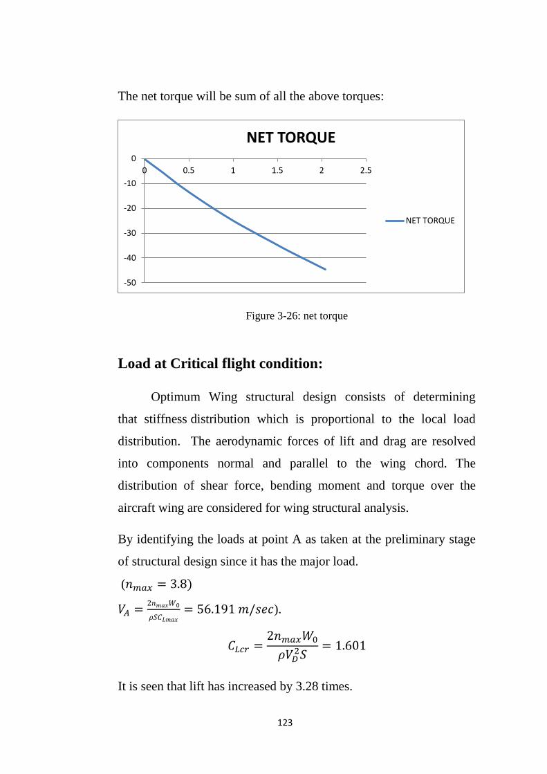
211
The net torque will be sum of all the above torques:
Figure 3-26: net torque
Load at Critical flight condition:
Optimum Wing structural design consists of determining
that stiffness distribution which is proportional to the local load
distribution. The aerodynamic forces of lift and drag are resolved
into components normal and parallel to the wing chord. The
distribution of shear force, bending moment and torque over the
aircraft wing are considered for wing structural analysis.
By identifying the loads at point A as taken at the preliminary stage
of structural design since it has the major load.
( )
𝑥
𝑆 𝑥
𝑠 ).
𝑆
It is seen that lift has increased by 3.28 times.
-50
-40
-30
-20
-10
0
0 0.5 1 1.5 2 2.5
NET TORQUE
NET TORQUE

211
So we introduce a constant of proportionality for the lift alone.
Figure 3-27: Linear lift distribution
Figure 3-28: elliptical load distribution
The aim is to find the shear forces and bending moments due to
normal forces in critical flight condition. There are two primary
loads acting on a wing structure in transverse direction which can
cause considerable shear forces and bending moments on it. They are
as follows:
Lift force (given by Schrenk‘s curve)
Self-weight of the wing
Now, the proportionality constant influences the lift force alone and
other factors remain unaffected.
0
200
400
600
800
1000
0 0.5 1 1.5 2 2.5
Linear lift distribution
0
500
1000
1500
2000
2500
3000
0 0.5 1 1.5 2 2.5
Elliptic
Elliptic

211
Figure 3-29: shrenk's for critical condition
Shear force and bending moment diagrams due to loads
along transverse direction at critical condition:
𝑆 ∫ ,
𝑦 - 𝑥 ................................................... (3-82)
𝑆 ∫ , 𝑥 √ 𝑥
(𝑥 ) - 𝑥
0
200
400
600
800
1000
1200
1400
1600
1800
-3 -2 -1 0 1 2 3
schrenk's

211
Figure 3-30:shear force
Bending moment:
∬,
𝑦 - 𝑥 ....................................... (3-84)
∬, 𝑥 √ 𝑥
(𝑥 ) - 𝑥
Figure 3-31: bending moment
-3500
-3000
-2500
-2000
-1500
-1000
-500
0
500
1000
0 0.5 1 1.5 2 2.5
SHEAR FORCE(CRITICAL LOAD)
SF(CA)
SF(BC)
FILLET-1
-500
0
500
1000
1500
2000
2500
3000
3500
4000
0 0.5 1 1.5 2 2.5
BENDING MOMENT(CRITICAL LOAD)
BM(CA)
BM(BC)

212
Torque at critical flight condition:
Torque due to normal force:
⁄ (
) ................................................ (3-85)
the equation for chord can also be represented in terms of x by taking
c= mx +k:
( 𝑥 𝑥 𝑥)
Therefore torque:
∫ 𝑥
∫( 𝑥 𝑥 𝑥) 𝑥
Figure 3-32: torque due to normal force for critical condition
-25
-20
-15
-10
-5
0
0 0.5 1 1.5 2 2.5
Torque due to normal force
Series1
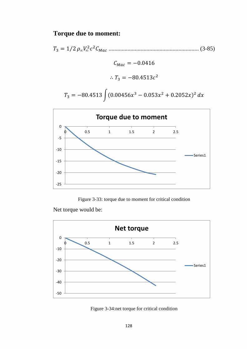
213
Torque due to moment:
⁄ .............................................................. (3-85)
∫( 𝑥 𝑥 𝑥) 𝑥
Figure 3-33: torque due to moment for critical condition
Net torque would be:
Figure 3-34:net torque for critical condition
-25
-20
-15
-10
-5
0
0 0.5 1 1.5 2 2.5
Torque due to moment
Series1
-50
-40
-30
-20
-10
0
0 0.5 1 1.5 2 2.5
Net torque
Series1

Chapter 4 : STABILITY
ANALYSIS

210
4.1 Introduction:
When an aircraft cruises, it is desirable that it do so at constant speed
and incidence, so the controls are at a fixed setting. Aircraft stability
is the study of how an aircraft responds to small disturbances in
flight and how it can be designed so that it remains at a fixed
incidence and speed without overworking the pilot. [9]
4.2 Static stability:
The static stability is the initial tendency of the vehicle or aircraft
to return to its equilibrium state after a disturbance, so the vehicle
must develop a restoring force and/or moment which tends to bring it
back to equilibrium condition.
4.2.1 Longitudinal Static stability:
The aircraft trim longitudinally if moment about the center of
gravity in Y axis zero, and has static longitudinal stability if any
disturbance in pitch direction (vertical direction) develops restoring
moment to trim position and that done if the aircraft had positive
and negative
, the aircraft will response to any disturbance
as shown below:
Figure 4-1 : aircraft response to pitch disturbance

212
The data which result from analysis from the DATCOM show that
the trim angle of attack = 4.2° and
Figure 4-2: Pitching Moment coefficient against angle of attack
4.2.2 Directional static stability:
Static directional stability is a measure of aircraft‘s ability to
realign itself along the direction of the resultant wind so that
disturbance in sideslip is effectively eliminated. Therefore, on
encountering a disturbance in the horizontal plane, the aircraft
orientation in space change but its heading remains the same to the
earth as shown in figure 4.3
Figure 4-3: aircraft orientation on horizontal plane
An air plane said to be directionally stable if it has positive yaw
moment coefficient and positive
.
-0.4
-0.2
0
0.2
-10 0 10 20
Pitching Moment coefficient against angle of attack
Pitching Moment

211
Figure 4-4:yaw moment coefficients against angle of attack
4.2.3 Lateral static stability:
Lateral stability is the inherent capability of the airplane to
counter a disturbance in bank; the airplane is neutrally stable with
respect to a disturbance in bank without sideslip, the sideslip
generate by horizontal weight component. If the sideslip develops
restoring moment the airplane said to be laterally stable .The rolling
moment that developed by sideslip is known as dihedral effect. The
airplane be laterally stable i.e. has positive dihedral effect if has
negative slope
.
Figure 4-5: rolling moment coefficient against sideslip angle
-0.6
-0.4
-0.2
0
0.2
0.4
0.6
-10 -5 0 5 10
Yaw Moment coefficient
Yaw Moment
-1
-0.5
0
0.5
1
-10 -5 0 5 10
Roll Moment
Roll Moment

211
4.3 Dynamic stability (Modes of Vibration):
In static stability analysis we examined the moments brought
about immediately after the disturbance. However a system is said to
be dynamically stable if it finally returns to the equilibrium position.
Hence to examine the dynamic stability we must analyze the
subsequent motion. The motion following an intended control input
or a disturbance is called response. Obtaining the response in the
case of airplane is an involved task.
4.3.1 Longitudinal Modes (Steady Modes of Vibration):
To examine the dynamic stability of the aircraft, we examine
the full longitudinal equations of motion. The longitudinal motion of
an airplane (controls fixed) disturbed from its equilibrium flight
condition is characterized by two oscillatory modes of motion.Figure
4.6 illustrates these basic modes. We see that one mode is lightly
damped and has a long period. This modecalled the long period
or phugoid mode. The second basic mode is heavily damped and has
a very short period; it is appropriately called the short-period mode.
Figure 4-6:phugoid and short period motions

211
4.3.1.1 Short Period Mode:
This Mode is characterized by change in angle of attack with
constant forward speed. It has a relatively big real part the
damping is thereforebig. The complex part is relatively big as
well. So the frequency is high. In other words, we have a highly
damped high-frequency oscillation. This motion is known as the
short period oscillation.
4.3.1.2 Long Period Mode (Phugoid):
This Mode is characterized by changes in pitch attitude,
altitude, and velocity at a nearly constant angle of attack. It has
a small real part , and therefore a small damping.The complex part
is small as well, so the frequency is low. In other words, we have a
lightly dampedlow-frequency oscillation. This motion is known as
the phugoid.
4.3.1.3 Longitudinal Modes Excitation:
Since the longitudinal stability modes are usually well
separated in frequency, it is Possible to excite the modes more or less
independently for the purposes of demonstration or measurement.
Indeed, it is a general flying qualities requirement that the modes be
well separated in frequency in order to avoid handling problems
arising from dynamic mode coupling.
The modes may be excited selectively by the application of a
sympathetic elevator input to the trimmed aircraft. The methods
developed for in-flight mode excitation reflect an intimate
understanding of the dynamics involved and are generally easily
adapted to the analytical environment. Because the longitudinal

211
modes are usually well separated in frequency the form of the input
disturbance is not, in practice, very critical. However, some
consistency in the flight test or analytical procedures adopted is
desirable if meaningful comparative studies are to be made.
Short period Excitation:
The short period pitching oscillation may be excited by
applying a short duration disturbance in pitch to the trimmed aircraft.
This is best achieved with an elevator pulse having duration of a
second or less. Analytically this is adequately approximated by a unit
impulse applied to the elevator. The essential feature of the
disturbance is that it must be sufficiently short so as not to excite the
phugoid significantly.
Long period Excitation:
The phugoid mode may be excited by applying a small speed
disturbance to the aircraft in trimmed flight. This is best achieved by
applying a small step input to the elevator which will cause the
aircraft to fly up, or down, according to the sign of the input.
4.3.2.1 Roll Subsidence Mode (periodic roll):
occur when the airplane does not possess directional or
weathercock stability. If such an airplane is disturbed from its
equilibrium state, it will tend to rotate to ever-increasing angles
ofsideslip. Owing to the side force acting on the airplane, it will fly a
curved path at large sideslip angles.

211
4.3.2.2 Spiral Mode:
Spiral divergence is a non-oscillatory divergent motion
which can occur when directional stability is large and lateral
stability is small. When disturbed from equilibrium, the airplane
enters a gradual spiraling motion. Thespiral becomes tighter and
steeper as time proceeds and can result in a high-speed spiral dive if
corrective action is not taken.
4.3.2.3 Dutch Roll Mode:
The Dutchroll mode is a classical damped oscillation in yaw,
about the OZ axisof the aircraft, which couples into roll and, to a
lesser extent, into sideslip. Themotion described by the Dutch roll
mode is therefore a complex interaction betweenall three lateral–
directional degrees of freedom. Its characteristics are described bythe
pair of complex roots in the characteristic polynomial.
Fundamentally, the Dutchroll mode is the lateral–directional
equivalent of the longitudinal short period mode.
Both the damping and stiffness in yaw, which determine the
characteristics of themode, are largely determined by the
aerodynamic properties of the fin, a large fin beingdesirable for a
well behaved stable Dutch roll mode. Unfortunately this contradicts
therequirement for a stable spiral mode.
4.3.2.4 Lateral Modes Excitation:
Unlike the longitudinal stability modes the lateral–
directional stability modes usually exhibit a significant level

212
of dynamic coupling and as a result it is more difficult to
excite the modes independently for the purposes of
demonstration or measurement.However, the lateral–
directional stability modes may be excited selectively by
thecareful application of a sympathetic aileron or rudder
input to the trimmed aircraft.
Because the lateral–directional stability modes usually
exhibit a degreeof dynamic coupling, the choice and shape
of the disturbing input is critical to themode under
investigation.
Roll subsidence mode:
The roll subsidence mode may be excited by applying a short
duration square pulse to the aileron, the other controls remaining
fixed at their trim settings. The magnitude and duration of the pulse
must be carefully chosen if the airplane is not to roll too rapidly
through a large attitude change and thereby exceed the limit of small
perturbation motion. Since the mode involves almost pure rolling
motion only no significant motion coupling will be seen in the
relatively short time scale of the mode. Therefore, to see the classical
characteristics of the roll subsidence mode it is only necessary to
observe roll response for a few seconds.
Spiral mode:
The spiral mode may be excited by applying a small step input
to rudderζ, the remaining controls being held at their trim settings.

213
The aero-plane responds by starting to turn, the wing on the inside of
the turn starts to drop and sideslip develops in the direction of the
turn.
Spiral mode:
Ideally, the Dutch roll mode may be excited by applying a doublet to
the rudder pedals with a period matched to that of the mode, all other
controls remaining at their trim settings.
4.4 Flying Qualities:
Flight qualities of an airplane are related to the stability and
control characteristics and can be defined as those stability and
control characteristics that important in forming the pilot‘s
impression of the airplane. The pilot forms subjective opinions about
the ease or difficulty of controlling the airplane in steady and
maneuvering flight. [10].
The dynamic stability characteristics are used to evaluate the flying
qualities of the airplane in the Cooper and Harper rating scale.
The evaluation of flying qualities rates the results in three levels:
• Level 1: flying qualities clearly adequate for the mission flight
phase
• Level 2: flying qualities adequate to accomplish the mission flight
phase, but with an increase in pilot workload and, or, degradation in
mission effectiveness
• Level 3: degraded flying qualities, but such that the aircraft can be
controlled, inadequate mission effectiveness and high or limiting
pilot workload.

214
Table 10: Aircraft Class
Class
I
Small, light airplanes, such as light utility, primary
trainer, and light observation craft
Class
II
Medium-weight, low-to-medium maneuverability
airplanes, such as heavy utility/search and rescue, lighter
medium transport/cargo/tanker, reconnaissance, tactical
bomber, heavy attack and trainer for Class II
Class
III
Large, heavy, low-to-medium maneuverability
airplanes, such as heavy transport/cargo/tanker, heavy
bomber and trainer for Class III
Class
IV
High-maneuverability airplanes, such as
fighter/interceptor, attack, tactical reconnaissance,
observation and trainer for Class IV
4.4.1 Longitudinal Flying qualities:
The longitudinal response characteristics of an airplane are
related to its stability derivatives. Because the stability derivatives
are related to the airplane‘s geometric and aerodynamic
characteristic it is possible for the designer to consider flying
qualities in the preliminary design phase.
4.4.1.1 Long Period Mode
Upper and lower values for phugoid frequency are not quantified.
However, it is recommended that the phugoid and short period mode
frequencies are well separated. It is suggested that handling
difficulties may become obtrusive if the frequency ratio of the
modes/ωs≤0.1. Generally the phugoid dynamics are acceptable

210
provided the mode is stable and damping ratio limits are quantified
as shown in Table (4.2).
Table 11: Long Period Mode damping ratio limits
Long period
Level 1 ξ > 0.04
Level 2 ξ > 0
Level 3 T > 55s
4.4.1.2 Short Period Mode
Acceptable limits on the stability of the short period mode are
quantified in terms of maximum and minimum values of the
damping ratio as a function of flight phase category and level of
flying qualities as set out in Table 10.4.The maximum values of short
period mode damping ratio obviously imply that actable non-
oscillatory mode is acceptable, table (4.3).
Table 12: Short period
Short period
level
ξ ξ
Min. Max.
1 0.35 1.30
2 0.25 2.00
3 0.15 -

212
4.4.2 Lateral Directional flying qualities:
4.4.2.1 Spiral mode flying qualities:
A stable spiral mode is acceptable irrespective of its time constant.
However, since its time constant is dependent on lateral static
stability (dihedral effect) the maximum level of stability is
determined by the maximum acceptable roll control force. Because
the mode gives rise to very slow dynamic behavior it is not too
critical to handling unless it is very unstable.
Table 13: Spiral mode- time to double amplitude
Class Category Level 1 Level 2 Level 3
I and IV A 12 s 12 s 4 s
B and C 20 s 12 s 4 s
II and III All 20 s 12 s 4 s
4.4.2.2 Roll mode flying qualities:
Since the roll subsidence mode describes short term lateral dynamics
it is critically important in the determination of lateral handling
qualities. For this reason the limiting acceptable values of its time
constant are specified precisely as listed in Table 4.5
.

211
Table 14: Roll mode – time constant
Class Category Level 1 Level 2 Level 3
I, IV A 1.0 1.4 10
II, III 1.4 3.0
All B 1.4 3.0 10
I, IV C 1.0 1.4 10
II, III 1.4 3.0
4.4.2.3 Dutch roll flying qualities:
Since the Dutch roll mode is a short period mode it has an important
influence on lateral–directional handling and, as a consequence, its
damping and frequency requirements are specified in some detail. It
is approximately the lateral–directional equivalent of the longitudinal
short period mode and has frequency of the same order since pitch
and yaw inertias are usually similar in magnitude.
Table 15: Dutch roll damping at frequency requirement
level Min ξ Min Min
1 0.19 0.35 1.0
2 0.02 0.05 0.4
3 0.02 - 0.4

211
4.5 Tools to estimate stability derivatives:
4.5.1 USAF DATCOM
4.5.1.1 Introduction to USAF DATCOM:
In preliminary design operations, rapid and economical
estimations of aerodynamic stability and control characteristics are
frequently required. The extensive application of complex automated
estimation procedures is often prohibitive in terms of time and
computer cost in such an environment. Similar inefficiencies
accompany hand-calculation procedures, which can require
expenditures of significant man-hours, particularly if configuration
trade studies are involved, or if estimates are desired over a range of
flight conditions. The fundamental purpose of the USAF Stability
and Control Dotcom is to provide a systematic summary of methods
for estimating stability and control characteristics in preliminary
design applications. Consistent with this philosophy, the
development of the Digital Dotcom computer program is an
approach to provide rapid and economical estimation of aerodynamic
stability and control characteristics.
The Digital DATCOM program uses aircraft-unique
configuration and geometry parameters to predict aircraft
performance by utilizing classical aerodynamic equations. The
Digital DATCOM program calculates static stability, high lift and
control, and dynamic derivative characteristics, and is applicable to
subsonic, transonic, supersonic, and hypersonic vehicles, for
traditional body-wing-tail or canard-equipped vehicles.

211
4.5.1.2 Using DATCOM:
The first step is to generate an input file in text format, its good
practice to just modify ready input file. For detail information about
input file the manual is suggested. Second is to execute the input
file, there are number of output files but the most important is one
with (.OUT) format. This file contains the estimated aerodynamic
and stability derivative.
4.5.2 Advance Aircraft Analysis (AAA):
4.5.2.1 Introduction to Advance Aircraft Analysis:
Advanced Aircraft Analysis (AAA) is the industry standard
aircraft design, stability, and control analysis software. AAA is
installed in over 55 countries and is used by major aeronautical
engineering universities, aircraft manufacturers, and military
organizations worldwide.
Advanced Aircraft Analysis provides a powerful framework to
support the iterative and non-unique process of aircraft preliminary
design. The AAA program allows students and preliminary design
engineers to take an aircraft configuration from early weight sizing
through open loop and closed loop dynamic stability and sensitivity
analysis, while working within regulatory and cost constraints.

Chapter 5 :
MATHMATICAL
MODELING OF UAV
DYNAMICS

211
5.1 Introduction:
This chapter gives an introduction to aircraft modeling. The
equations of motion are derived then linearized using small
perturbation theory and the final results are state-space models for
the longitudinal and lateral motions. The models can be used for
aircraft simulation and design of flight control systems.
5.2 Definition of coordinate system:
There are mainly three forces that act upon UAV during flight
this are aerodynamic, Gravitational, and Thrust forces. This Forces
together with linear and angular velocities need to be defined with
appropriate coordinate system. Three basic coordinate system often
used in UAV modeling it will be defined next.
5.2.1 Inertial Reference Frame:
The inertial reference frame is fixed on a point on the Earth‘s
surface and is aligned so that the positive X axis points to true North
and the positive Y axis points to true East. The z axis points down
and is normal to the surface of the Earth. This frame is commonly
referred to as the North-East-Down, or NED frame. [11]
5.2.2 Body Fixed coordinate Frame:
The aircraft body frame‘s origin is fixed at the aircraft‘s center
of gravity. The body frame has its X axis aligned with the nose of the
aircraft so that the aircraft‘s nose points in the positive X direction.
The positive Y direction points out along the aircraft‘s starboard
wing. The z axis points down to complete a right handed coordinate
frame. Figure (5.1) below defines Body Fixed coordinate Frame

211
Figure 5-1: Body Fixed coordinate Frame
The body reference frame can assume any orientation with respect to
the inertial frame. The orientation of the body frame with respect to
the inertial frame is usually described by an Euler sequence of
rotations. The ordering of the rotations is critical to the orientation of
the body frame. [11]
5.2.3 Wind and Stability Reference Axis:
Wind Axis: This reference frame has origin fixed to the
vehicle, usually at the mass center C, and the 𝑧 axis is
directed along the velocity vector V o f the vehicle relative to
the atmosphere.The axis 𝑧 lies in the plane of symmetry of the
vehicle if it has one, otherwise is arbitrary.
Stability axes: are a special set of body axes used
primarily in the study of small disturbances from a steady reference
flight condition[12]

212
5.3 Rigid Body Equation of Motion:
The Rigid body equation of motion are obtained from
newton's second low of motion, which states that the summation of
all eternal forces acting on body is equal to the time rate of change of
the momentum of the body; and the summation of the external
moments acting on the body is equal to the time rate of change of the
moment of momentum. The time rate of change of linear and angular
momentum is referred to an absolute or inertial reference frame[10].
∑F =
( ) …………………………………………………(5-1)
∑M =
………………………………………..……………(5-2)
The vector equation can be rewritten in scalar form and then consist
of three force equation and three moment equation. The force
equation can be expressed as follows:
( 𝑢)
( 𝑣)
( 𝑤)…………………(5-3)
Where , and u, v, w are the component of force and velocity
along x, y and z axis respectively. The force components are
composed of contributions due to the aerodynamic, propulsive and
gravitational forces.
The moment equations can be expressed in a similar manner:
……………………………(5-4)
Where L, M, N and , , are the component of the moment and
moment of momentum along x, y and z axis respectively.

213
If we take as an element of mass of aircraft, v be the velocity of
the elemental mass relative to an absolute or inertial frame, and δF
be the resulting force acting on the elemental mass then newton‘s
second low yields
Figure 5-2:Rigid Body Equation of Motion
=
……………………………………………………(5-5)
And the total external force acting on the airplane is found by
summing all the elements of the airplane
………………………………………………………(5-6)
The velocity of deferential mass is
𝑣
…………………………………………………(5-7)
where is the velocity of the center of mass of the airplane
and dr/dt is the
velocity of the element relative to the center of mass.
Substituting this Expression for the velocity into Newton‘s second
law yields
∑ 𝑡 ∑( 𝑟 𝑡) ……………………(5-8)

214
If we assume that the mass of vehicle is constant equation (5-8) can
be rewritten as
F = m
+
∑
……………………………………….(5-9)
∑𝑟 …………………………………. (5-10)
Because r is measured from the center of mass, the summation ∑ r
m is equal to zero. The force equation then becomes
…………………………………………………(5-11)
which relates the external force on the airplane to the motion
of the vehicle‘s center of mass. In a similar manner, we can
develop the moment equation referred to a moving center of
mass. For the differential element of mass, m, the moment
equation can be written as
( ) ……………………(5-12)
The velocity of the mass element can be expressed in terms of
the velocity of the center of mass and the relative velocity of the
mass element to the center of mass:
V =
𝑟 …………………………………(5-13)
where is the angular velocity of the vehicle and r is the
position of the mass element measured from the center of mass.
The total moment of momentum can be written as
∑ ∑ ( 𝑟 ) ∑ [𝑟 ( 𝑟) …(5-14)
The velocity is a constant with respect to the summation
and can be taken outside the summation sign

210
∑𝑟 ∑ [𝑟 ( 𝑟) ……………………(5-15)
The first term in Eq. (5-15) is zero because the term ∑𝑟 = 0, as
explained previously. If we express the angular velocity and position
vector as
𝑝 𝑞 𝑟 …………………………………………… (5-16)
And
𝑟 𝑥 𝑦 𝑧 ……………………………………………(5-17)
Then after expanding Eq. (5-15), H can be written as
(𝑝 𝑞 𝑟 )∑(𝑥 𝑦 𝑧 ) ∑(𝑥 𝑦 𝑧 )(𝑝𝑥
𝑞𝑦
𝑟𝑧) ……………………………………………………………….
(5-18)
The scalar components of H are
𝑝 ∑(𝑥 𝑦 ) 𝑞 ∑𝑥𝑦 𝑟∑𝑥𝑧 …………. (5-19)
𝑝 ∑𝑥𝑦 ∑(𝑥 𝑦 ) 𝑟 ∑𝑦𝑧 (5-20)
𝑝 ∑𝑥𝑧 𝑞 ∑𝑦𝑧 𝑟 ∑(𝑥 𝑦 ) ………(5-21)
The summations in the above equations are the mass moment
and products of inertia of the airplane and are defined as
follows:
∫ ∫ ∫ ( (𝑦 𝑧 ) ∫ ∫ ∫ 𝑥𝑦 ……………(5-22)
∫ ∫ ∫ ( (𝑥 𝑧 ) ∫ ∫ ∫ 𝑥𝑧 ……………. (5-23)
∫ ∫ ∫ ( (𝑥 𝑦 ) ∫ ∫ ∫ 𝑦𝑧 ……………(5-24)

212
The terms , and are the mass moments of inertia of the
body about the x, y and z axes, respectively. The terms with the
mixed indices are called the products of inertia. Both the moments
and products of inertia depend on the shape of the body and the
manner in which its mass is distributed. The larger the moments
of inertia the greater the resistance the body will have to
rotation. The scalar equations for the moment of momentum are
given below
𝑝 ……………………………………. (5-25)
𝑝 𝑞 𝑟 …………………………………... (5-26)
𝑝 𝑞 𝑟 …………………………………... (5-27)
If the reference frame is not rotating then, as the airplane
rotates, the moments and products of inertia will vary with time.
To avoid this difficulty we will fix the axis system to the
aircraft (body axis system). Now we must determine the
derivatives of the vectors v and H referred to the rotating body
frame of reference. It can be shown that the derivative of an
arbitrary vector A referred to a rotating body frame having an
angular velocity can be represented by the following vector
identity:
|
| ……………………………………….. (5-28)
where the subscript I and B refer to the inertial and body
fixed frames of reference. Applying this identity to the equations
derived earlier yields
| ( ) ……………………………….. (5-29)

211
| ………………………………………... (5-30)
(�� 𝑞𝑤 𝑟𝑣 ) (�� 𝑟𝑢 𝑝𝑤) (𝑤 𝑝𝑣 𝑞𝑢
………………………………………………………………... (5-31)
𝑞 𝑟 𝑟 𝑝 𝑝 𝑞
……………………………………………………….…….… (5-32)
The components of the force and moment acting on the airplane are
composed of aerodynamic, gravitational, and propulsive
contributions. By proper positioning of the body axis system,
one can make the products of inertia . To do
this we are assuming that the XZ plane is a plane of symmetry of the
airplane. With this assumption, the moment equations can be written
as
�� 𝑞𝑟( ) 𝑝𝑞 …………………… (5-33)
�� 𝑟𝑝( ) (𝑝 𝑟 ) ……………………. (5-34)
�� �� 𝑝𝑞( ) 𝑞𝑟 …………………. (5-35)
5.4 linearization using Small-perturbation theory:
The equations developed in the previous section can be
linearized by using small-disturbance theory. In applying small
disturbance theory we are assuming that the motion of the airplane
consists of small deviations about a steady flight condition.
Obviously, this theory cannot be applied to problems in which large
amplitude motions are to be expected (e.g. Spinning or stalled
flight).However, in many cases small disturbance theory yields
sufficient accuracy for practical engineering purposes.

211
All the variables in the equations of motion are replaced
by a reference value plus a perturbation or disturbance:
𝑢 𝑢 𝑢𝑣 𝑣 𝑣𝑤 𝑤 𝑤
𝑝 𝑝 𝑝𝑞 𝑞 𝑞𝑟 𝑟 𝑟
…………….. (5-36)
For convenience, the reference flight condition is assumed to be
symmetric and the propulsive forces are assumed to remain constant.
This implies that
……………………… (5-37)
Furthermore, if we initially align the x axis so that it is along the
direction of the airplane‘s velocity vector, then 𝑤 = 0
Now, if we introduce the small disturbance notation into the
equations of motion, we can simplify the equations of motion. With
appropriate derivation will result in the linearized small disturbance
longitudinal Equation:
(
) 𝑢 𝑤 ( 𝑜𝑠 𝜃 ) 𝜃 (5-38)
𝑢 (( )
)) 𝑤 ((𝑢 )
𝑠𝑖 𝜃 )) 𝜃
…………………………………………………......… (5-39)

211
𝑢 (
) 𝑤 (
) 𝜃
………………………………………………………………... (5-40)
The linearized small disturbance Lateral Equation:
(
) 𝑣 𝑝 (𝑢 ) 𝑟 ( 𝑜𝑠 𝜃 ) 𝜑 (5-
41)
𝑣 (
) 𝑝 (
) 𝑟 ....
(5-42)
𝑣 (
) 𝑝 (
) 𝑟
.(5-43)
5.5 Aerodynamic and stability Derivatives
5.5.1Longitudinal Derivatives:
5.5.1.1 Derivative due to change in forward speed,
u( ):
The drag, lift and pitching moment vary with changes in the
airplane‘s forward speed. In addition the thrust of the airplane is also
a function of the forward speed. The aerodynamic and propulsive
forces acting on the airplane along the X body axes are the
drag force and the thrust. The change in the X force can be
expressed as:
𝑢
𝑢
𝑢 …….................................... (5-44)

211
……................................................................ (5-45)
The derivative
is called the speed damping derivative.
…….................................................................... (5-46)
……............................................................... (5-47)
…….............................................................................. (5-48)
Since Our UAV had low Mach number this derivatives have
no significant affect.
Derivative due to change in Pitching Velocity, q ( , ):
The stability coefficients and represent the change in
the Z force and pitching moment coefficients with respect to the
pitching velocity q.
……............................................................. (5-48)

211
Pitch Damping Derivative : This derivative is normally negative,
and determines the moment that opposes any pitch rate. It provides
the most important contribution to the damping of the dynamic
behavior in pitch and hence is intimately involved in aircraft
handling qualities. The pitch damping is not given by the slope of an
aerodynamic coefficient; it must be estimated from oscillatory
motion of the aircraft or aircraft model, or calculated.[13]
…….......................................................... (5-49)
Derivative due to change of ( , ):
The stability coefficients and arise because of the lag
in the wing downwash getting to the tail. As the wing angle of attack
changes, the circulation around the wing will be altered. The change
in circulation alters the downwash at the tail; however, it takes a
finite time for the alteration to occur.
𝜂
……...................................................... (5-50)
𝜂
…….................................................. (5-51)
Equations (5-50) and (5-51) yield only the tail contribution to
these stability coefficients. To obtain an estimate for the
complete airplane these coefficients are increased by 10 percent.

212
Derivative due to the Rolling rate, p ( 𝐩, 𝐩 𝐩):
The stability coefficient , arise due to the rolling
angular velocity,p.When an airplane rolls about its longitudinal axis,
the roll rate creates a linear velocity distribution along the vertical,
horizontal and wing surfaces. The velocity distribution causes a local
change in angle of attack over each of this surfaces that result in a
change in the lift distribution and consequently the moment about
center of gravity[10]
𝑡 …..................................................... (5-52)
……........................................................................ (5-53)
……............................................................... (5-54)
Derivative due to the Yawing rate, r ( , ): The
stability coefficient , are caused by yawing angular
velocity, r. A yawing rate causes a change in the side force acting on
the vertical tail surface.
(
)( ) ……..................................................... (5-55)
𝜂 (
)
.................... (5-56)

213
5.6 State variable representation of the equations of
motion:
The linearized longitudinal equations developed in Chapter 3
are simple, ordinary linear differential equations with constant
coefficients. The coefficients in the differential equations are made
up of the aerodynamic stability derivatives, mass, and inertia
characteristics of the airplane. These equations can be written as a set
of first-order differential equations. When the equations are written
as a system of first-order differential equations they are called the
state-space or state variable equations and are represented
mathematically as
............................................................................. (5-57)
Where x is the state vector, s the control vector and the matrices A
and B contain the aircraft‘s dimensional stability derivatives
The linearized longitudinal equations developed earlier are
repeated below.
In practice, the force derivatives and are usually neglected
because they contribute very little to the aircraft response. Therefore,
to simplify our presentation of the equations of motion in the state
space form we will neglect both and . Rewriting the equations
in the state-space form yields

214
[
�� �� ��
��
] [
𝑢
𝑢
] *
𝑤 𝑞 𝜃
+
[
] [
]
where the state vector x and control vector are given by
𝑥 *
𝑤 𝑞 𝜃
+ 𝜂 [
]
and the matrices A and B are given by
[
𝑢
𝑢
]
[
]
From [nelson]:
𝜆 …….................................................... (5-58)
√ ……..................................................................... (5-59)
( )
√ ……....................................................................(5-60)
𝑟𝑖𝑜
……...................................................................(5-61)

210
𝑡 𝑜𝑟 𝑡
| | ……................................................. (5-62)
Lateral-directional equations of motion:
The lateral-directional equations of motion consist of the side
force, rolling moment and yawing moment equations of motion. The
lateral equations of motion can be rearranged into the state space
form in the following manner. We start with Eq. (5.27) shown below.
(
) (𝑢 ) 𝑟 𝑜𝑠𝜃 …...
(5-63)
(
) (
) 𝑟 .....
(5-64)
(
) (
) 𝑟 ..(5-
65)
Rearranging and collecting terms the above equations can be
written in the state variable form:
…….................................................................... (5-66)

212
The matrices A and B are defined as follows:
[
(𝑢 )
𝜃
]
[
]
𝑥 [
𝑟
]And𝜂 [
]
From [nelson]:
√ ……...................................................................... (5-67)
√ ……........................................................................... (5-68)

Chapter 6 : UAV
DYNAMICS
MODELING USING
SIMULINK

211
6.1 Introduction:
In Chapter II the full nonlinear equations of motion were
developed and in Chapter III the complete set of stability and control
derivatives were obtained. Now the next step is to develop the model
of the aircraft on a Matlab Simulink.
6.2 UAV Dynamic Modeling:
UAV modeling has been part of the design and modification
process for new UAVs and has increasingly been used for rapid
testing and verification. Changes and modifications are made to the
model, evaluating it for intended function against the requirement.
Modeling allows a faster verification and iteration of the design
change cycle without having to conduct a flight test with a prototype
UAV. It also reduces the cost incurred for each design change.
6.2.1 Nonlinear Model:
Nonlinear aircraft simulations are useful for dynamic analysis,
control law design and validation, guidance and trajectory studies,
pilot training, and many other tasks. (Nonlinear AC Simulations in
MATLAB)
The nonlinear models contain three basic models:
1) Aerodynamic Model: Contains forces and moments that act on
aircraft during flight, the equation used to estimate these forces
and moments are defined at each model below since it depends on
degrees of freedoms of the model.
2) Atmosphere model: since Dynamic pressure is necessary to
estimate aerodynamic forces and moment, therefore air density at
each altitude is also required. For this purpose, the ‗ISA
Atmosphere Model ' model will be used. A description of this
idealized model of the earth's atmosphere can, for instance.
3) Engine Model: For simplicity engine thrust is assumed to be
constant for all altitude and forward flight speed.
4) Gravity Model: The gravitational force acting on the airplane acts
through the center of gravity of the airplane. Because the body
axis system is fixed to the center of gravity, the gravitational
force will not produce any moments. It will, however,

211
contribute to the external force acting on the airplane and
will have components along the respective body axes.
6.2.1.1 Three Degree of freedom Longitudinal Model:
Figure 6-1:Three Degree of freedom Longitudinal Model
The three degree of freedom Longitudinal Model is
composed of the following blocks:
Equation of motion Block: this block is taken from aerospace block
set and is used to solve three degree of freedom longitudinal
equation, the equation is as follows:
( )
𝑞𝑤 𝑠𝑖 𝜃 ………………..…...…. (6-1)
𝑤
𝑞𝑢 𝑜𝑠 𝜃 ………………………. (6-2)
𝑞
……………………………………………. (6-3)

211
𝜃 𝑞 ………………………………………………... (6-4)
Aerodynamic Block:
The aerodynamic block is shown below:
Figure 6-2: aerodynamic block
The component of this block as follows:
Lift coefficient block
……………… (6-5)
The lift model is shown in Figure (6-3) below
Figure 6-3: Lift coefficient block

211
The drag coefficient block:
( )
…….... (6-6)
Figure 6-4: Drag coefficient block
Moment Coefficient block:
…………… (6-7)
Figure 6-5: Moment Coefficient Block

212
Atmospheric Model:
Figure 6-6: Atmospheric Model
The angle of attack is calculated from
𝑡
………………………………………... (6-8)
6.2.1.2 Three Degree of freedom Lateral Model:
In similar manner to longitudinal Model the lateral Model
construction is shown:
Figure 6-7: Three Degree of freedom Lateral Model

213
Three Degree of freedom Lateral equation of motion is modeled
using Simulink block set, these equation are defined as:
��
𝑢𝑟 𝑠𝑖 𝜑 …………………… …….…. (6-9)
��
………………..……………………….…... (6-10)
��
……………………………………………... (6-11)
�� �� …………………………………………….. (6-12)
�� ………………………………….………….. (6-13)
This equation of motion is modeled as:
Figure 6-8: Lateral Equation of motion
Aerodynamic Forces and Moments:
𝑞𝑠 ……………………….…………………..(6-14)
𝑞𝑠 …………………………………………....(6-15)
𝑞𝑠 …………………………………………..(6-16)

214
Figure 6-9: Aerodynamic Forces and Moments
Aerodynamic Forces and Moments Coefficient are calculated (a/c
from dynamic to simulation)
( 𝑝 𝑟) ..(6-17)
( 𝑝 𝑟) …. (6-18)
( 𝑝 𝑟) (6-19)

220
For instance, Coefficient is modeled as in Figure (6-10)
Figure 6-10:C_y Coefficient Block
The other coefficients ( ) are modeled in the same
manner.
6.2.1.3 Six Degree of freedom Model:
This Model is a result of coupling three degree of freedom
longitudinal and lateral models into one six degree of freedom
model. The model is shown in Figure (6-11).

222
Figure 6-11: Six Degree of freedom Model
Calculation of equation of motion requires the definition of tensor
matrix as follows:
*
+ (6-20)
Atmospheric Model
Figure 6-12: eAtmospheric Model
6.3 Aerodynamic Model:
To calculate aerodynamic and moments the following model is
constructed.

221
Figure 6-13: Aerodynamic and moment of Six DOF model
The Aerodynamics forces & Moments are in wind axis system to
transfer it into body axis system; we will need to the following
transformation matrix (DCM):
[
𝑜𝑠 𝑜𝑠 𝑜𝑠 𝑠𝑖 𝑠𝑖 𝑠𝑖 𝑜𝑠
𝑠𝑖 𝑜𝑠 𝑠𝑖 𝑠𝑖 𝑜𝑠 ]………….. (6-21)
Gravity Model: obtained from reference [nelson].figure (6-14) below
[
𝑠𝑖 𝜃 𝑠𝑖 𝜃 𝑠𝑖 𝜑 𝑜𝑠𝜃 𝑜𝑠𝜑
]……………………... (6-22)
Figure 6-14: Gravity Model

221
6.2.2 Linear Model:
Linear is constructed using state space models derived in the
previous chapter.
6.2.2.1 Three Degree of freedom Longitudinal Model:
Figure 6-15: Three DOF Linear Longitudinal Model
6.2.2.2 Three Degree of freedom Lateral Model:
Figure 6-16: Three DOF Linear Lateral Model

Chapter 7 : PROPELLER
DESIGN

221
AERODYNAMIC DESIGN
7.1 Theories comparison
As it was seen before propeller is made of number of blades
which made of some airfoils arranged in such manner to compose
blade, when this blade rotate it will create lift and drag which lead to
create thrust and torque. That blade must be arranged in specific
shape according to aerodynamics lows and equations.
In this chapter aerodynamics theories and equations shall be
discussed and there comparison between them to choose one of
theory for design and then aerodynamics design will be achieved.
Those theories are[14]:
1. Momentum theory
2. Blade element theory
7.1.1 Momentum theory:
Momentum theory does not use blade shape or airfoil shape
for design, there are many assumptions for this theory like:
a. Propeller assumed to replace by actuator disk energizer.
b. The disk assumes to be very small thickness and is continuous
and 100% porous of no mass. With projectedا frontal area A
(swept area) to the annulus of rotating propeller blade.
c. There is no resistance (i.e. drag) of the air pressure through
actuator disc (since there are no propeller blade).
d. The axial velocity through the disc is uniform over actuation
area and considered to be smooth across the disc, i.e. no abrupt
change is experienced.
e. The received energy manifests itself in working medium (i.e. air)
finally in form of differential pressure ( ) a jump change

221
across the actuator disc uniformly distributed across the disc
surface.
f. The fluid medium (air) assumed to be perfect in compressible
fluid flow is irrotational in front of and behind disc but not
through it.
g. The static pressure far from the disc, i.e. far upstream and
downstream, are both assumed equal atmospheric pressure, the
corresponding velocity are independent value , to be determine
separately.
Figure 7-1: Momentum theory
Advantages of the theory:
Easy to calculate.
Disadvantages of the theory:
1. Thrust assumed to be generated by actuator disc not by blade so
that there is not consideration of interference between blades,
propeller chord, length and angle of the blade.
2. It considers there is not drag generated by the propeller.

222
3. Velocity through disc assumed to be constant but that is not true
because of the appearance of blade sections.
7.1.2 Blade element theory:
A relatively simple method of predicting the performance of a
propeller (as well as fans or windmills) is the use of Blade Element
Theory. The primary limitation of the momentum theory is that it
provides no information as to how the rotor blades should be
designed so as to produce a given thrust. Also, profile drag losses are
ignored. The blade-element theory is based on the assumption that
each element of a propeller or rotor can be considered as an airfoil
segment. Lift and drag are then calculated from the resultant velocity
acting on the airfoil, each element considered independent of the
adjoining elements.
This produces a set of non-linear equations that can be solved
by iteration for each blade section. The resulting values of section
thrust and torque can be summed to predict the overall performance
of the propeller.
Disadvantages of the theory:
The theory does not include secondary effects such as 3-D
flow velocities induced on the propeller by the shed tip vortex or
radial components of flow induced by angular acceleration due to
rotation of the propeller. In comparison with real propeller results
this theory will over-predict thrust and under-predict torque with a
resulting increase in theoretical efficiency of 5% to 10% over
measured performance. Some of the flow assumptions made also
breakdown for extreme conditions when the flow on the blades

223
becomes stalled or there is a significant proportion of the propeller
blade in wind milling configuration while other parts are still thrust
producing.
Advantages of the theory:
The theory has been found very useful for comparative studies
such as optimizing blade pitch setting for a given cruise speed or in
determining the optimum blade solidity for a propeller. Given the
above limitations it is still the best tool available for getting good
first order predictions of thrust, torque and efficiency for propeller
under a large range of operating conditions. All equations will be
explained later.
Figure 7-2: propeller blade sections
7.2 Aerodynamic calculations:
In this part, the aerodynamic calculation of the propeller will be
achieved.
For the given data of the propeller and engine many parameters must
be estimated such as:

224
Propeller diameter, propeller pitch angle, propeller chord line, thrust
produced by propeller, power consumed by propeller and propeller
drag.
7.2.1 Propeller diameter
Diameter is the most important parameter of the propeller and
it effects directly in propeller performance. As diameter increase,
thrust produced by propeller increased and power consumed by
propeller will increase also, but the efficiency of the propeller will
decrease.
There are many parameters must be taken into consideration in
diameter calculation such as:
1. Space between two tail booms.
2. The height of the propeller from the earth.
3. Engine characteristics (such as engine horsepower and engine
rpm).
7.2.2 Diameter calculation:
𝑟𝑝
𝑟 𝑠
To prevent stall propeller tip Mach number must be less than 1
√ √ 𝑠

230
=
= 0.295 m , D=2R = 2
Also, there is many other ways and equations used to calculate aircraft
propeller diameter[8] such as:
1. D = 22 √
…………………………………………….(7-1)
D = 22 √
𝑖 & r = 0.562 m
2. D =
√
……………………………..………(7-2)
=
√( )= 0.585 m, r = 0.2925 m
From the above equations it seems , there are many values for
aircraft propeller diameter, but value which estimated by equation
(7-2) will be taken as a value of aircraft propeller diameter because it
takes many parameters into consideration , ensures better strength
and satisfy the aircraft design requirements.
Note: this diameter is equivalent to the length of wing span, as the
propeller rotates an induced roll moment is generated. We further
explore the possibility of using counter-rotating blades. Counter-
rotating blades have mainly two advantages: they are more efficient
at high Mach numbers than a single propeller configuration and they
allow a smaller diameter blade, allowing them to spin at higher rpm
without a loss in aerodynamic efficiency. By having counter-rotating

232
blades, our propeller diameter will be decreased considerably while
maintaining the same efficiency.
7.3 Design envelops:
In this section, design of aircraft propeller will be done
depending on the engine characteristics such as engine rpm and
horsepower, and aircraft Specifications like aircraft cruise speed,
Maximum speed and distance between the tail booms. Propeller
design includes calculation of the length of chord line at each
section, drag and lift generated at each section and power consumed
by aircraft propeller[15].
To fulfill these objectives there are many parameters should be
known previously.
7.3.1 Airfoil selection:
Due to the high Mach number, compressibility effects
(recompression shocks, causing additional drag) reduce the
efficiency of the propeller. A practical way to keep the drag of an
airfoil at acceptable levels is the use of thinner and less cambered
airfoils, to avoid excessive drag.
The airfoils selected were the CLARK–Y, NACA6412, MH 114 and
NACA9412 because the characteristics that met the design
constraints.
The first step while carrying out a propeller design to choosing an
airfoil is looking into the airfoil characteristics such as the L/D ratio,
the maximum CL, stall angle depending on the desired thickness as
well.

231
Table16: airfoil characteristics comparisons
MH 114 NACA
9412
NACA
6412
CLARK-Y
0.13c
0.12c 0.12 c 0.117c Thickness
0.6c
0.09c 0.06c 0.034c Camber
11.8deg
13.7deg 14.2deg 15.3deg Trailing
edge angle
.808c
.381c .812c
.718c Lower
flatness
1.981
2.148 1.785 1.295 Max CL
12.0 12.0 12.0 8.5 Max CL
angle
.27c .17c .17c .12c Leading
edge radius
46.291 58.12 60.34 51.61 Max L/D
6.5 0.5 4.0 7.0
Max L/D
angle
1.676 1.229 1.268
1.18 Max L/D
CL
12.0deg
12.0deg 4.0deg
8.5deg Stall angle
-8.0deg -9.5deg -6.0deg -3.5deg
Zero-lift
angle

231
The proper airfoil selected is Clark-y
Figure 7-3: Clark-y airfoil
There are many types of airfoil used for propeller design like NACA
16 series and Clark-Y airfoils, NACA 16 series usually use in
designing of propeller with engines which have horse power greater
than 700 hp so that Clark-Y
Airfoil was selected for this project. The airfoil has a maximum
thickness of 11.7 percent of the chord at 30 percent of chord back
and is flat on the lower surface .The flat bottom simplifies angle
measurements on propellers, for many applications the Clark Y has
been adequate; it gives reasonable overall performance in respect of
its lift-to- drag ratio, and has gentle and relatively benign stall
characteristics .But the flat lower surface is sub-optimal from an
aerodynamic perspective, and it is rarely used in new designs.
From lift and drag curve (fig 7.3) below which plotted against of
attack it is found that ( =10 degree) is the best angle of attack for
Clark-Y airfoil which gives maximum lift to drag ratio
(CL/CD=14.667).

231
Figure 7-4: Clark-y lifte and drag curve
7.3.2 Number of Blades, B:
There are many parameters must be taken in consideration at
the number of blade selection, like engine horsepower, diameter of
the propeller and chord length of the propeller. The most efficient
propellers are two bladed. Because the diameter of propellers is so s
mall, multiple blade propellers disturb the air that the trailing blade is
entering. Therefore, 3 and 4 blade propellers are less efficient.
7.4 Calculation method and iteration:
In this section of the project, calculation method and iteration will be
discussed, all calculations and iteration will be achieved according to
the blade element theory with iteration method because there are
many parameters need initial guessed values, and the last value will
be obtained from iteration as explained below :

231
Iteration method
1. Firstly, solution will start with some initial guessed values of
inflow factors (a) and (b) , apply this guessed values on equations ((7-3)
to (7-7)) to find the flow angle on the blade.
( )……………………………………………...…. (7-3)
ω ( )…………………………….………………..…. (7-4)
√ ………………………………………………… (7-5)
φ
……………….……………..…...…………………… (7-6)
𝜃 ( 𝜑)……………………………..………………………… (7-7)
2. The second step: chord length can be calculated by using equation
(7-9)
λ
………………..…………………….………………….. (7-8)
Figure 7-5: Blade element theory parameters

231
λ ……………………………………………….…….. (7-9)
3. Then use blade section properties to estimate the element thrust and
torque from equation (7-10) and (7-11) )
C ( 𝜑 𝜑) 𝑟……………...….... (7-10)
( 𝜑 𝜑(𝜑) ) 𝑟 𝑟…………. (7-11)
4. With these approximate values of thrust and torque equations (7-12)
and (7-13) can be used to give improved estimates of the inflow
factors (a) and (b).
𝑟 ( ) 𝑟…………………………………………… (7-12)
𝑟 ( ) 𝑟……………...………………………. (7-13)
5. This process can be repeated until values for (a) and (b) have
converged to within a specified tolerance; this process must be used for
blade sections separated from each other.
For the final values of inflow factor (a) and (b) an accurate prediction of
element thrust and torque will be obtained from equations (7-10) and
(7-11).
C ( 𝜑 𝜑) 𝑟…………..…..….. (7-10)
( 𝜑 𝜑(𝜑) ) 𝑟 𝑟…………. (7-11)
6. The overall propeller thrust and torque will be obtained by
summing the results of all the radial blade element values.

232
The non-dimensional thrust and torque coefficients can then be
calculated along with the advance ratio at which they have been
calculated.
( )………………………………………...……….. (7-14)
And
( )………………………………………………… (7-15)
For
( )…………………….……………………………….. (7-16)
Where n is the rotation speed of propeller in revs per second and D is
the propeller diameter.
The efficiency of the propeller under these flight conditions will then
be:
( ) ( )…………………………………….. (7-17)
Design condition and assumption:
In this part of project many assumption and values of
parameter will be explained. This value taken from the aircraft
specification engines description and airfoil characteristics and will
take as constant values it will not change through this project.

233
Table17: Design condition and assumption
Value Dimension symbol Parameter NO
10 Degree α Angle of attack 1
1.1 - Lift coefficient 2
0.075 - Drag coefficient 3
47 m/sec Maximum aircraft
speed
4
2980 Rpm N Maximum
revolution per
minute
5
16.4 Hp HP Engine power 6
0.585 M D Propeller diameter 7
Sea level Design condition 8
The equations states above from (7-3) to (7-15) were programmed in
MATLAB Software code.
The result of this code are reasonable and realistic, at the root of the
propeller the chord length is 0.1443 m and the pitch angle is 1.1369
RAD ( 65.14 deg).at the tip of the propeller the chord length 0.0295 m
and the pitch angle is 0.3294 RAD( 18.87 deg).All the results are
scheduled in the tables below:

234
Symbol for iteration :
Section 1 r = 0.02925 m
An θ 𝜑 N
O
0.01 0.02
38
0.44
97
10.0
811
1.13
94
0.96
49
0.14
54
1
0.01
88
0.01 0.43
56
9.81
61
1.13
72
0.96
27
0.14
45
2
0.01
4
0.00
98
0.43
51
9.81
29
1.13
69
0.96
24
0.14
43
3
Table18: Results of iteration for all sections of propeller
R An 𝛉 𝝋 NO
0.02925 0.014 0.0098 0.4351 9.8129 1.1369 0.9624 0.1443 1
0.0585 0.0044 0.0208 0.8419 21.1474 0.7956 0.6210 0.1020 2
0.08775 0.0019 0.0321 1.2351 32.9721 0.6229 0.4484 0.0767 3
0.117 0.0010 0.0437 1.6111 45.3174 0.5241 0.3495 0.0612 4
0.14625 0.00063640 0.0554 1.9683 58.2064 0.4612 0.2866 0.0511 5
0.1755 0.00042759 0.0675 2.3063 71.6892 0.4180 0.2435 0.0440 6
0.20475 0.00025452 0.0702 2.0567 74.6897 0.3727 0.1982 0.0339 7
0.234 0.00021644 0.0906 2.7994 98.2262 0.3608 0.1862 0.0342 8
0.26325 0.00016900 0.1054 3.1848 115.8586 0.3443 0.1697 0.0319 9
0.2925 0.00013109 0.1186 3.4294 131.9649 0.3294 0.1548 0.0295 10

240
∑ ( 𝑜𝑟 𝑡𝑠)
∑ ( 𝑜𝑟 𝑡𝑠)
= ( ) = 0.137
( ) ( ) =
0.00704
( ) ( ) 0.438
( ) ( ) 0.438/2 (0.137 / 0.00704) = 1.36
The total torque required to drive propeller, power required and
activity factor can be calculated by equations (7-18),(7-19) and (7-
20) as shown below:
∫
…………………………….. (7-18)
∫
∫
………….………………. (7-19)
∫
=15.64 KW

242
Activity factor (AF) is a design parameter associated with the
propeller blades geometry
AF=
∫
𝑟
. …………………………………… (7-20)
AF=
∫
𝑟
.dr = 19
The more slender the blade (larger radius, smaller chord), the lower
the AF value
JAVAPROP is a simple tool for the design and the analysis of
propellers and wind turbines .Within its limits, it is applicable to
aeronautical as well as to marine applications. The implemented
classical blade element design and analysis methods are based on a
coupling of momentum considerations with two-dimensional airfoil
characteristics. It is therefore possible to consider different airfoil
sections and the impact of their characteristics on rotor
performance.
JAVAPROP contains a powerful direct inverse design module.
Inverse design means that specify only a few basic parameters and
Java Foil produces a geometry which automatically has the
maximum efficiency for the selected design parameters. The
beautiful thing is that JAVAPROP creates an optimum propeller with
just 5 design parameters plus a selection of airfoil operating points
along the radius.

241
7.5 Cascade design:
7.5.1 Stage with downstream guide vanes:
This arrangement is shown in figure (7.5) below. The rotor
blades receive air in the axial direction. The absolute velocity vector
at the rotor exit has swirl component which is removed by the
downstream guide vanes (DGVs) and the flow is finally discharged
axially from the stage.
The design start firstly by estimate the propeller stage parameters:
stage work, stage reaction, stage pressure rise.
Figure 7-6: Axial propeller stage with downstream guide vanes

241
Figure 7-7: Axial propeller stage with downstream guide vanes (velocity
triangles for R<1 )
The swirl at the entry to the rotor is zero ( =0).
The work done in the stage:
= ( )
The stage pressure rise:
( ) ( )
Therefore the stage pressure coefficient:
= ( )
The pressure rise in the rotor:

241
( )
Stage reaction:
( )
As the propeller rotation speed is 2100 rpm so,
𝑠
, , 𝑠
( )
( )
( ) ( )
(
)
= ( ) ( )
( )
=1.225
( )=
( tan )
Secondly, by take these parameters in consideration.
The cascade system is a number of guide vanes (2 to 8), the choice of
guide vanes depending on the number of rotor blades and the area of
actuation.

241
In this procedure, the best choice for 2-rotor blades is 4 guide
vanes has the same of some of the specifications of the blade such
as, airfoil selection is Clark-y ,each two guide vanes with the hub
diameter like propeller diameter. This arrangement is shown in
figure (7.7) below:
7.6 Co-axial propeller design:
In this section, the coaxial propeller system is made by using the
same procedure of the above design to design the lower rotor (the
second propeller), by take in consideration the opposite setting angle
of the propeller. The critical distance between the two propellers
assume to be as the chord length at tip
The coaxial rotor design offers many advantageous attributes over
singular rotor systems.
Figure7-8: Cascade arrangement

241
Figure 7-9: Flow Model of a Co - Axial Rotor System
Co-axial advantages:
1. Directional stability through cancellation of torque moment (Yaw
torque reaction)
2. Compact size through use of concentric shafts.
3. Increased pressure differential over rotor system; increased thrust,
higher efficiency for increase in thrust, which translates into a
reduction in rotor diameter for a given thrust.
4. High thrust to weight ratio
5. Absence of torque transfer
6. Precession load are balanced
7. Freedom from propeller size limitations.

242
8. Complete symmetry of rotor system.
9. Simplified rotor system.
10. Freedom from control cross-coupling
11. Optimal transmission design
Disadvantages:
1. They can be very noisy, with increases in noise in the axial
(forward and aft) direction of up to 30 dB, and tangentially 10
dB.
2. Inter- rotor wash interference. Reduced efficiency of the lower
rotor due to the upper rotor swirling the air in the opposite
direction of the lower rotor which requires the lower rotor to run
at higher speed to produce the same lift as the upper rotor.
3. Importance of flow interaction, requirement for rotor spacing. To
ensure sufficiently clean flow for the lower disc, the spacing must
be wide enough to allow as little interaction of the swirl of the
upper rotor to impinge on the retreating component of the lower
disc.
7.7 Practical calculations:
To evaluate the value of static thrust on each case, practical
experiments were done. By running the motor, the propeller started
to suck the air. The manometer used to estimate the value of dynamic
pressure.

243
Figure 7-10: Pitot-tube and the manometer
As the K.E =
𝑣
…………………………………………….……….……….. (7-21)
The pressure from the manometer:
P= ………………………………………………….….… (7-22)
As p is a K.E (dynamic pressure), is the height of water inside
the manometer
So;
√
……………………………………….…..….. (7-23)
,
T = ( )…………………………………………. (7-24)
For static thrust , T = ,

244
( ) =0.269
=
, 1864 watt
FOR SIGLE PROPELLER:
The manometer measure h=11 mm =0.011m
√
𝑠
T=
= 43.39
FOR SIGLE PROPELLER WITH REARWARD CASCADE:
By setting the cascade blade at 5 deg, the manometer measure
h=14.5 mm =0.0145m
√
𝑠
T=
= 65.74
By setting the cascade blade at 10 deg, the manometer measure h=18
mm =0.018m
√
𝑠

100
T=
= 90.87
By setting the cascade blade at 15 deg, the manometer measure
h=16.5mm =0.0165m
√
𝑠
T=
= 79.82
FOR COAXIAL PROPELLER: the manometer measure h=18.7
mm =0.0187m
√
𝑠
T=
= 96.259

Chapter 8 :
FABRICATION

101
Propeller fabrication method:
One of the key goals of this work was to automate as much of the
fabrication process as possible.
The needed to fabrication start when propeller needed to run
experiment aims to reduce the effect of swirl flow.
The needed propeller chosen to made by casting but first must make
wood model to prepare the cast.
The wooded propeller was made by method of carving propellers
with helical pitch [16]as showing in the blow picture:
Figure 8-1: propeller layout

101
Figure 8-2: Propeller curving
And by using sample carpentry tools as show below:
Figure 8-3: carpentry tools

101
Figure 8-4: Propeller wooden model
Then the propeller had been casted and surface finished as showing
below:
Figure 8-5: Propeller casting

101
Figure 8-6: Surface finishing
Figure 8-7: Final product

101
After that there was need to test section to collect the air flow and its
made from sheet of alminium rolled as a duct, the duct also used to
support the fixed cascade, and to get continous test section with high
unformity flow with minimum disturbance, to achieve that the shaft
should extend, but the long shaft lead to high vibrations and bending
loads this need front bearig support as showing in figure below:
Figure 8-8: System modifications

102
The cascade is the first method of reduceing swirl generated by the
propeller and made from four wooden blade and used screw and nuts
to judging the blade angle.
Figure 8-9: Cascade blades
The last step was to use coaxial propellers and this required
additional propeller with opposite pitch relative to the first one and
fabricated by wood due to the load acting on the electrical motor by
propeller weight and friction load from the gear box.
Figure 8-10: Coaxial system

103
The tools which used to measure the motor and propeller RPM & the
flow velocity is optical digital tachometer and pitot tube with
manometer respectively.
Figure 8-11: Optical digital tachometer
Figure 8-12: Pitot tube with manometer

Chapter 9 : RESULTS &
DISCUSION

120
Aerodynamics:
The approach conducted to calculate the aerodynamic coefficients is a
crude mean to follow. It assumes that the laminar flow is about 10% of
the total flow and turbulent flow is about 90%.
Figure 9-1: lift curve slope
Figure 9-2: drag against angle of attack
-1
-0.5
0
0.5
1
1.5
2
-10 -5 0 5 10 15 20 25
Lift
Lift
0.00E+00
2.00E-02
4.00E-02
6.00E-02
8.00E-02
1.00E-01
1.20E-01
1.40E-01
-10 -5 0 5 10 15 20 25
Drag
Drag

122
Figure 9-3: Pitching Moment
Figure 9-4: Roll Moment
-0.4
-0.3
-0.2
-0.1
0
0.1
0.2
-10 -5 0 5 10 15 20
Pitching Moment
Pitching Moment
-0.6
-0.4
-0.2
0
0.2
0.4
0.6
-10 -5 0 5 10
Roll Moment
Roll Moment

121
Figure 9-5: aw Moment
Figure 9-6: side force coefficient against beta
-0.6
-0.4
-0.2
0
0.2
0.4
0.6
-10 -5 0 5 10
Yaw Moment
Yaw Moment
-4
-3
-2
-1
0
1
2
3
4
-10 -5 0 5 10
Side Force Cofficient aginst beta
Side Force Cofficient Withbeta

121
Figure 9-7: alpha against Epslon
Figure 9-8: alpha against d_Epslon
Performance analysis:
The power required &power available curve define the maximum &
minimum speeds. The maximum speed is about
𝑠 which exceeds the required maximum speed. This is
considered as a positive indication to the performance of UAV.
The stall speed is found to be5 26.6 m/s while the required stall speed is
about 28 m/s which is beyond the required speed. The landing distance
-2
-1
0
1
2
3
4
5
-10 -5 0 5 10 15 20 25
Alpha aginst Epslon
Alpha aginst Epslon
-0.5
-0.4
-0.3
-0.2
-0.1
0
0.1
0.2
0.3
0.4
-10 -5 0 5 10 15 20 25
Alpha aginst d_Epslon
Alpha aginst d_Epslon

121
is about which is beyond the required landing distance. The
take-off distance is about as seen to be less than the required
take-off distance. These characteristics serve to optimize performance
characteristics.
Structure analysis of fuselage:
V-n diagram has been drawn based on CS-VLA (UAV standard
requirements) as considered the first step to initialize structural design.
The maximum load factor for positive angle of attack is 3.8 and for
negative angle of attack is -1.5, while the maximum dive speed as
The gust diagram which defines the loads originating from
sudden increase of speed winds has been constructed with gust speed of
15.24 m/s for . Loads on the fuselage have been regarded as inertia
loads exerted by the various weights on the fuselage (payload, landing
gear, fuel, fixed equipment & fuselage weight itself), where a pull down
condition is taken to be our design condition since the major loads are
likely to occur there. By constructing the shear & bending moments
diagrams depending on the loads and their distribution, a design position
along the fuselage is selected as the maximum value of each (
𝑡 𝑥 𝑡). Structure layout
has been selected from previous UAVs noticing that the stringer
distribution happened to be at the edges of the cross section of the
maximum load, in order to assist in reacting the direct stressing on the
skin of the structure. The simple bending moment theory has been
adopted for analytical calculation of stress and shear flow. The results
obtained from these calculations as shown in table (6).
𝑞

121
𝑞
𝑞
𝑞
𝑞
𝑞
Depending on these values, the required skin thickness happened to be
1mm. Zed-section stringers has been selected and the results of sizing
them have shown that:
𝑡
𝑤
Structure analysis of wing:
The structural design of the wing is followed according to the Shrenk's
load distribution along span which is a combined approach of linear and
elliptic load distribution on the wing as shown in figure (34).
In addition to the shrenk's load, self-weight of the wing is regarded. It is
the parabolic distribution of the weight of the wing itself as shown in
figure (36).
Depending on the summation of the shrenk's load and self weight
distribution, the shear and bending diagrams were obtained as first
integral & second integral with respect to position along span as shown
in figure (45), &figure (46).
The torque on the wing is also considered. It originates on this project
from two sources (normal force and moment), which are dependent on
the angle of attack as shown in figure (47) & figure (48).

121
The critical loading is assigned for point A as it's considered at the
preliminary stage of structural design. The lift & drag coefficient were
increased by 3.28. This shall absolutely affect the shrenk's and self-
weight loads & consequently the shear & bending moment diagrams.
The load resulted from the torque is affected due to variation with
normal force and the moment as shown in fig(49).
Stability analysis:
Static stability results:
The static stability analysis is estimated with DATCOM the output
together with the discussion is as follows:
Longitudinal static stability:
From DATCOM results in figure (51)
are negative and equal to -0.8
Trim angle of attack equal to
Directional Stability:
From figure (53) :
The slop is Positive hence the UAV is directionally stable
Lateral Static Stability from figure (54)
The slop is negative as required hence the UAV is
directionally stable.
Complete Definition of stability& control derivatives:
The stability derivatives estimated using two software tools
DATCOM & AAA, The result is shown on table below:

122
Table 20: Stability derivatives
Coefficients DATCOM AAA
0.024 0.02304
0.344 0.3789
0.1034 0.1139
5.6149 5.2181
0.17188 0.1607
-0.7563 -0.8281
-3.655 -4.2
CYB -0.4262 -0.8575
CNB 0.05872 0.3178
CLB -0.0575 -0.0785
CLP -0.4878 -0.0105
CYP -0.01994 -0.0013
6.383 6.8487
-31.16 -33.6478
- 0
CNR -0.0965 -0.2814
CLR 0.191 0.1266
CYR - 0.6121
Cdαdot - 0
Clαdot - 1.4698
Cybeta dot - -0.2297
Clbeta dot - -0.0006
Clu - 0.0078
Cmu - 0.0001
Cdu - 0.0

123
Verification:
Table 1 has a summary of stability coefficients and aerodynamic
characteristics of the UAV calculated by both AAA & DATCOM.
In general, the longitudinal aerodynamics coefficients computed by
DATCOM agree well with these ones estimated by AAA. Excellent
correlations are achieved for the lift, Drag & Moment at zero angle of
attack.
The Longitudinal stability coefficients ( , & ) agree well
with the two method. But Lateral derivatives are very different, the
reason of this might be:
1. As the DATCOM can‘t take twin boom configuration, we were
urgency to assume one vertical tail. This will strongly affect
lateral directional stability derivatives.
2. After literature survey on lateral stability estimation and
verification, we found that lateral directional derivatives are
always different and harder to correlate with different estimation
methods.
3.
State space results
Using Matlab code in appendix ().the state space of both longitudinal
and lateral equation of motion are solved. The eigenvalues of the state
matrix are as follows:
Eigenvalues of the longitudinal states:
𝜆
𝜆

124
By examining theeigenvalues:
There are two pairs of complex conjugate eigenvalues.
Both pairs of eigenvalues have negative real parts. This means
that the UAV is stable.
Parameter Short period Long period
-0.0012
0.0482
0.363 575
period 1.537s 130.356
Number of cycles to
half-amplitude
0.2366 cycles 4.418
Eigenvalues of the lateral states:
𝜆
𝜆
𝜆
By examining the eigenvalues:
There are two real eigenvalues and one pair of complex conjugate
eigenvalues.
The UAV thus has three modes of vibration.
There is a positive eigenvalue. The aircraft is thus unstable. But
since the eigenvalue is small the UAV will diverge slowly.
𝜂

110
𝑡 𝑠
Period = 1.376s
Number of cycles to half-amplitude = 0.684cycles
Flying Qualities:
The dynamic stability characteristics are used to evaluate the
flying qualities of the airplane in the Cooper and Harper rating scale.
The flying qualities for all the modes of motion are excellent, rating in
Level 1 for the Cooper and Harper scale.
Lateral Directional flying qualities:
Roll subsidence flying qualities:
From AAA the Roll mode time constant is equal to:
Thus UAV achieved level one flying quality in Roll.
Spiral mode flying qualities:
From AAA software tool the time to half amplitude is found to be (3.85)
this approximately gives level three flying qualities.
Dutch roll flying qualities:
From Matlab code appendix ().the Dutch roll frequency and damping is
found as follows:

112
Thus from table () the Dutch roll is achieved level one flying qualities.
Mode EXCITATION:
Each mode is excited using appropriate control input. Table ()
shows how to excite each mode:
Table21: Model Excitation
Longitudinal Modes
Long Period (Phugoid) Elevator step
Short Period Elevator Impulse
Lateral Modes
a periodic roll Aileron square pulse
Spiral Rudder Step
Dutch Roll Rudder doublet
Nonlinear model:
Three Degree of freedom longitudinal model:
Initial condition:
m = 76.6532 kg
Initial velocity = 47 m/s
Initial body attitude (𝜃) = 0
Initial incidence ( )= 0
Initial body rotation rate (q) = 0
= 0

111
Response to Elevator Impulse:
As from above table elevator impulse used to excite short period
mode, it‘s difficult to separate short period from long period modes. The
short period is appearing in the first three second, while the long period
mode which is now is not of our interest appeared at 400 sec. The
elevator impulse is shown in figure () below
Figure 9-9: Response to Elevator Impulse
Alpha:
The Short period is obvious at first 3sec.
Figure 9-10: angle of attack

111
Pitch attitude:
The long period is obvious at pitch, and is running from 53sec till it
damped out at 400 sec. figure () show this discussion.
Figure 9-11: Pitch attitude
Pitch Rate:
Figure 9-12: Pitch Rate

111
Forward Speed (u):
Forward Speed varies as the pitch attitude the long period is
visible.
Figure 9-13: Forward Speed (u)
Speed (W):
The (w) is same as angle of attack (Alpha).
Figure 9-14: Upward Speed (w)

111
Response to Elevator Step:
As from table is used to excite Long period, the short period is
characterized by change in angle of attack with constant forward speed.
The elevator step is shown in figure (110) below:
Figure 9-15: Elevator Step of one degree
Alpha: from figure (111) the disturbance is damped at 250sec.
Figure 9-16: Alpha

111
Pitch attitude:
Figure 9-17: Pitch attitude
Pitch Rate:
Figure 9-18: Pitch Rate

112
U, W
Figure 9-19: U, W
From above result the following is noticed:
The short period and long period‘s modes are both stable.
9.4.2 Three Degree of freedom Lateral model:
Initial Conditions:
U = 47 m/s
𝜑 = 0
= 0
q = 0
= 0
= 0

113
Aileron Step:
The aileron step is used to excite Roll subsidence.
Beta:
Figure 9-20: Beta
Phi
Figure 9-21: Phi

114
Psi
Figure 9-22: Psi
Roll Rate:
Figure 9-23: Roll Rate

110
V:
Figure 9-24: V
Yaw Rate:
Figure 9-25: Yaw Rate

112
Rudder Step:
Beta
Figure 9-26: Beta
Phi:
Figure 9-27: Phi

111
Psi:
Figure 9-28: Psi
Roll Rate:
Figure 9-29: Roll Rate

111
Yaw Rate
Figure 9-30: Yaw Rate
Rudder Impulse
Beta
Figure 9-31: Beta

111
PHI
Figure 9-32: PHI
Psi
Figure 9-33: Psi

111
Roll Rate
Figure 9-34: Roll Rate
Yaw Rate
Figure 9-35: Yaw Rate

111
V
Figure 9-36: V
General discussion of Lateral model results:
The Roll mode is stable
The spiral Mode is stable
Six degree of freedom Model:
Elevator Impulse
Alpha
Figure 9-37: Alp

112
Euler Angles
Figure 9-38: Euler Angles
p , q , r
Figure 9-39: p , q , r

113
U , V , W
Figure 9-40: U , V , W
Linear Model:
Three degree of freedom Longitudinal:
Elevator Impulse
q
Figure 9-41: q

114
Theta
Figure 9-42: Theta
u
Figure 9-43: u

110
w
Figure 9-44: w
Elevator Step
q
Figure 9-45: q

112
Theta
Figure 9-46: Theta
u
Figure 9-47: u

111
w
Figure 9-48: w
Three Degree of Freedom Lateral Model:
Aileron Step
Beta
Figure 9-49: Beta

111
PHI
Figure 9-50: phi
Roll Rate
Figure 9-51: Roll Rate

111
Yaw Rate
Figure 9-52: Yaw Rate
Rudder Impulse
Beta
Figure 9-53: Beta

111
PHI
Figure 9-54: phi
Roll Rate
Figure 9-55: Roll Rate

111
Yaw Rate
Figure 9-56: Yaw Rate
`
PROPELSION SYSTEM RESULTS:
Diameter calculation:
Equation (7-1) gives D = m and the value is too much higher
than that calculate from equation (7-2) because it consider only the
engine horse power but the value of equation (7-2) is reasonable to
avoid tip shock waves
Chord calculation:
The only available equation for calculate the chord is (7-9) but it
give unreasonable distribution of chord through root to tip.

112
.
Propeller model:
The first wooden model of propeller gives weak results such as
(lower RPM , lower flow field distribution) . this weak results cured
by change the blade angle .the second model give a good results.
because that the overall efficiency of a counter-rotating propeller is
not seriously affected by changes in rotational speed or small
changes in blade angle of the aft propeller disk. These changes did,
however, have a moderate effect when the propeller was operated at
peak efficiency.
Propeller fabrication:
Due to the lack of welding joints between the rearward propeller and
outer shaft on the coaxial system ,propeller separated from the
column. This can be solve by using a suitable welding joint
,manufacturing a new column of suitable material, or work to install
a good propeller.
Figure 9-57

113
Practical experimental:
Firstly the air density was taken because the test base at
altitude of 1000 m.
The power source was electrical motor with 2.5 horsepower with
2800 R.P.M and reduced by transmission unit to 1400 R.P.M due to
the high load of gearbox.
The propeller static thrust equal to and enhance by using
the cascade it clear that thrust increase first with increase of angle of
setting but it reduce again due to separation.
When coaxial propeller used, give high thrust compare with single
propeller because it almost cancels the swirl and the velocity
vector more straight.

Chapter 10 :
CONCLUSIONS &
RECOMMENDATIONS

114
Conclusion:
A UAV designed with the roadmap defined at the beginning of
the project with exceeding characteristics in performance and
stability. The material selected for structure of fuselage has a load
factor with a less margin of safety, reserving the integrity of
structure.
DATCOM was used to Compute the forces and moments, these
values were utilized to calculate the stability coefficients and
stability derivatives at a given flight condition. The negative values
of and and a positive , demonstrate that the airplane is
statically stable.
Dynamic stability was verified using Simulink, results in good
dynamic behavior. The longitudinal modes show convergent
oscillation.
The derivatives found by DATCOM were validated by AAA, no
significant differences were found between the longitudinal static
and dynamic stability analysis done by both DATCOM & AAA.
Where lateral directional stability were deference.
The dynamic stability characteristics are used to evaluate the flying
qualities of the UAV achieving level one flying qualities for short
period.
Dutch roll mode and roll mode of the airplane match with damped
mode and convergent mode, respectively. However, spiral mode
response prediction corresponds to a divergent mode. This means
their plane is dynamically unstable for spiral mode, and stable for
Dutch roll mode and roll mode.

110
According to the results from engine, following conclusions are
drawn:
The blade element theory method can be applied to any complicated
propeller configuration and determine the characteristics.
The Cascade and Coaxial system may raise the propeller efficiency
around 1-2 percent of design condition for the present system.
As the difference on thrust increase between the Cascade & Coaxial
system is very small, it is prefer logically and practically to avoid the
increase in weight and mechanism complexity, used the cascade
design.

112
Recommendations:
To ensure that a minimum induced drag could be obtained, a
further structural arrangement for installation of winglets should
be included.
Aerodynamics data obtained by Raymer is a crude mean of
estimation. Therefore, CFD analysis is needed.
At some point of design, the fuel was selected to be at the wings.
This was cancelled since the choice for installation the fuel in
fuselage had shown a better alternative. The calculations on wing
loads were based on positioning the fuel in it. So, it is needed
recalculation on base of being positioned in fuselage.
The material selected for fuselage structure had a small margin of
safety; it should be changed with a stiffer material. Composite
materials should be a design alternative with a provided theory to
calculate the stresses.
A stress analysis program such as NASTRAN PATRAN should
be used to verify stress analysis on structural components.
Run flight test to validate stability derivatives & identify the
mathematical model.
Design a control system for the UAV.
Lateral directional modes had shown middle dynamic behavior,
so it needs to be carefully studied.
Stability augmentation system is required to achieve a good
spiral & Dutch roll stability.
Develop Analysis program for CRPs which is able to capture the
thrust/torque characteristics in an averaged sense.
Use of simulation to observe various parameters that affect
propeller interference which can be helpful to optimize propeller
performance.
Use a suitable aerodynamic tool for propeller analysis such as
Panel methods and Computational Fluid Dynamics (CFD), etc. to
obtain valid animated aerodynamic results.

111
Modifying a new light weight mechanism that satisfying the
propeller operation by using suitable engine that give the require
power.
Make a visualization test to verify that the coaxial propeller
system cancel the swirl actually and make a smooth flow.
Composition a control system that regulate the engine RPM.
Complete the required four tests by using a forward cascade to
select wherever it gives a better performance.
Reduce the extra noise in the coaxial propeller system by enclose
the coaxial propeller in a shroud or by making a new design of
the two propellers has different blades (e.g.: use two blades on
the forward propeller & three on the aft).

References:
[1] R. Baylis, C. Collins, C. French, E. Pham, and A. Valiyff, "design and development of a tailless fuel cell powered Unmanned Aerial Vehicle," University of Adelaide
p. 247, 2009. [2] D. P. Raymer, Aircraft design: a conceptual approach: American Institute of
Aeronautics and Astronautics Reston, 2006. [3] J. Roskam, Airplane design: Roskam Aviation and Engineering Corporation, 1990. [4] J. Vanderover and K. Visser, "Analysis of a Contra-Rotating Propeller Driven
Transport Aircraft," AIAA Student Paper Competition, 2006. [5] S. C. Playle, K. Korkan, and E. Von Lavante, "A numerical method for the design and
analysis of counter-rotating propellers," Journal of Propulsion and Power, vol. 2, pp. 57-63, 1986.
[6] M. S. Farooque, "CFD Grid generation and flow analysis of a counter rotating open rotor propulsion system," The Ohio State University, 2010.
[7] M. H. Sadraey, "Aircraft Design A Systems Engineering Approach," p. 799, 2013. [8] J. Anderson, "Aircraft Performance And Design
" p. 600. [9] M. Carley, "Some nots on aircraft and spacecraft stability and control," p. 115. [10] R. C. Nelson, Flight stability and automatic control vol. 2: WCB/McGraw Hill, 1998. [11] M. A. K. Mark Peters, "The Engineering Analysis and Design of the Aircraft Dynamic
Model For the FAA Target Generation Facility," p. 321, 2012. [12] B. Etkin and L. D. Reid, Dynamics of flight: stability and control: Wiley New York,
1996. [13] B. L. S. a. F. L.Lewis, "Aircraft Control and Simulation," p. 680. [14] Rankine, "propeller theories," 1885. [15] F. E. Weick, "Aircraft propeller design," 1930. [16] K. D. WOODS, "Airplane design."
.

APPENDICIES:
APPENDIX A: WING AIRFOIL DATA
NACA2412


NACA 23012

.

NACA4415

FX61147

APPENDIX B: CLARK-Y CHARACTRISTICS

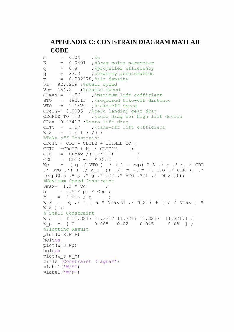
APPEENDIX C: CONISTRAIN DIAGRAM MATLAB
CODE m = 0.04 ;%µ K = 0.0401 ;%Drag polar parameter q = 0.8 ;%propeller efficiency g = 32.2 ;%gravity acceleration p = 0.002378;%air density Vs= 82.0209 ;%stall speed Vc= 154.2 ;%cruise speed CLmax = 1.56 ;%maximum lift cofficient STO = 492.13 ;%required take-off distance VTO = 1.1*Vs ;%take-off speed CDoLG= 0.0035 ;%zero landing gear drag CDoHLD_TO = 0 ;%zero drag for high lift device CDo= 0.03417 ;%zero lift drag CLTO = 1.57 ;%take-off lift cofficient W_S = 1 : 1 : 20 ; %Take off Constraint CDoTO= CDo + CDoLG + CDoHLD_TO ; CDTO =CDoTO + K .* CLTO^2 ; CLR = CLmax /(1.1*1.1) ; CDG = CDTO - m * CLTO ; Wp = ( q ./ VTO ) .* ( 1 - exp( 0.6 .* p .* g .* CDG
.* STO .*( 1 ./ W_S ))) ./( m -( m +( CDG ./ CLR )) .*
(exp(0.6 .* p .* g .* CDG .* STO .*(1 ./ W_S)))); %Maximum Speed Constraint Vmax= 1.3 * Vc ; a = 0.5 * p * CDo ; b = 2 * K / p ; W_P = q ./ ( ( a * Vmax^3 ./ W_S ) + ( b / Vmax ) *
W_S ) ; % Stall Constraint W_s = [ 11.3217 11.3217 11.3217 11.3217 11.3217] ; W_p = [ 0 0.005 0.02 0.045 0.08 ] ; %Plotting Result plot(W_S,W_P) holdon plot(W_S,Wp) holdon plot(W_s,W_p) title('Constraint Diagram') xlabel('W/S') ylabel('W/P')

APPENDIX D: PERFORMANCE ANALYSIS CODE
%Basic Configuration Parameters
W0 = 167.652 ;
Wf = 9.889176801085958 ;
S = 14.80812952 ;
P0 = 16.4 ;
g = 32.2 ;
c = 2.0202E-07 ;
mr = 0.4 ;%friction coefficient
j = 1.15 ;
n = 3 ;
%Aerodynamic Parameters
CLm = 1.655 ;
Cd0 = 0.034 ;
k = 0.0401;
Pinf = 0.002577 ;
Pinf1 = 1.225 ;
Palt = 0.0017556 ;
Eff = 0.8 ;%Propeller efficiency
theta = 0.0523598775598299 ;%3deg
%Calculating wing loading and power loading
W_S = W0 ./ S ;
P_W = P0 ./ W0 ;
%Calculating Power Required & Maximum Speed
Vs = sqrt( W_S ./ ( 0.5 .* Pinf .* CLm ) ) ;
Vinf = 80 : 10 : 380 ;
T_R = 0.5 .* Pinf .* Vinf.^2 .* S .* Cd0 + 2 .* k .* S
* ( W_S )^2 ./ ( Pinf .* Vinf.^2 ) ;
P_R = ( W0 ./ G1 ) .* sqrt( 2 .* W0 ./ ( Pinf .* S .*
Vinf.^2 ) ) ;
P_A = P0 .* ( Pinf ./ Palt ) ;
T_A =Eff .* P0 ./ 154.2 ;
%Calculating Lift to drag ratios
CL = 2 .* W_S .* g ./( Pinf .* Vinf.^2 ) ;
CD = Cd0 + k .* CL.^2 ;
L_D = 1 ./ sqrt( 4 .* k .* Cd0 ) ;%lift to drag ratio
max
CL_CD = 0.25 .* ( 3 ./ ( k .* Cd0^( 1 / 3 ) ))^( 3 / 4
);%CL^(1/2)/ CD
CLCD = 0.75 .* ( 1 ./ ( 3 .* k .* Cd0^( 3 ) ))^( 1 ./ 4
);%CL^(3/2)/CD
V1 = sqrt( ( 2 ./ Pinf ) .* sqrt( k ./ Cd0 ) .* W_S )
;
V2 = 0.76 .* V1 ;%Velocity at CL^(1/2)/ CD is max
V3 = 1.32 .* V1 ;%Velocity at CL^(3/2)/ CD is max

G = CL ./ CD ;
G1 = CL.^0.5 ./ CD ;
G2 = CL.^1.5 ./ CD ;
%Calculating RATE OF CLIMB AND CLIMB VELOCITY
h = 0 : 100 : 10000 ;
Pinf_h = 6.10 .* 10^-19 .* h.^4 - 7.10 .*10^-14 .* h.^3
+ 4.10 .* 10^-9 .* h.^2 - 10^-4 .* h + 1.225 ;
V_RC = sqrt( ( 2 ./ Pinf_h ) .* ( sqrt( k ./ ( 3 .*
Cd0 ) ) ) .* W_S .* 4.882427636 ) ;
RC = Eff .* P0 .* 76.04022 .* ( Pinf_h ./ Pinf1 ) ./
( W0 .* 0.45359237 ) - V_RC .* ( 1.155 ./ L_D ) ;
%Calculating BEST ANGLE AND RATE OF CLIMB
Vv = ( P0 .* Eff ./ ( W0 .* Vinf ) - ( P_R ./ ( W0 ) ) )
.* Vinf ;
R = ( Eff ./ c ) .* L_D .* log( W0 ./ ( W0 - Wf ) );
E = ( Eff ./ c ) .* sqrt( 2 .* Pinf .* S ) .* ( CLCD .*
( ( W0 - Wf )^-0.5 - ( W0 )^-0.5 ) ) ;
%Calculating landing distance
Vf = 1.23 .* Vs ;
R = Vf^2 ./ ( 0.2 .* g ) ;%Flight Path radius during
flare
hf = R .* ( 1 - cos( theta ) ) ;%Flare hight
Sa_L = ( 50 - hf ) ./ tan( theta ) ;%Approach distance
to clear 15.24 m obstacle
Sf_L = R .* sin( theta ) ;
Sg_L = j .* n .* sqrt( ( 2 ./ Pinf ) .* W_S .* ( 1 ./
CLm ) ) + j^2 .* ( W_S ) ./ ( g .* Pinf .* CLm .* mr ) ;
L = Sa_L + Sf_L + Sg_L ;
%Calculating take off distance
V = 0.77 .* Vs ;
TA = Eff .* P0 .* 550 ./ V ;
Rt = 6.96 .* Vs^2 ./ g ;%Flight Path radius during
flare
Theta = acos( 1 - ( 50 ./ R ) ) ;
Sg_T = 1.21 .* W_S ./ ( g .* Pinf .* CLm .* ( TA ./ W0
) ) ;
Sa_T =Rt * sin( Theta ) ;
TO = Sg_T + Sa_T ;
%%Plotting Result
figure(1)
plot(Vinf,P_R)
title('Power Required Curve')
xlabel('Velocity (ft/s)')
ylabel('PR')
%%Plotting Result
figure(1)
plot(Vinf,G)
holdon
plot(Vinf,G1)
holdon
plot(Vinf,G2)

title('Variation of lift to drag ratio Curves Versus
Velocity')
xlabel('Velocity (ft/s)')
ylabel('Lift to drag ratio Curves')
%%Plotting Result
figure(1)
plot(Vinf,T_R)
holdon
plot(Vinf,T_A)
title('Thrust Required & Thrust available Curve')
xlabel('Velocity (ft/s)')
ylabel('TR & TA')
%%Plotting Result
figure(1)
plot(Vinf,P_R)
holdon
plot(Vinf,P_A)
title('Power Required & Power available Curve')
xlabel('Velocity (ft/s)')
ylabel('PR & PA')
%%Plotting Result
figure(1)
plot(RC,h)
title('Rate of climb Curve')
xlabel('RCmax(ft/s)')
ylabel('Altitude (ft)')
%%Plotting Result
figure(1)
plot(V_RC,h)
title('Rate of climb velocity Curve')
xlabel('V_RC(ft/s)')
ylabel('Altitude (ft)')
%%Plotting Result
figure(1)
plot(Vinf,Vv)
title('Hodograph for climb performance')
xlabel('Vinf(ft/s)')
ylabel('Vv')

APPENDIX E: WING OPTMIZATION
clc clear N = 9; % (number of
segments - 1) S = 14.80812952; % m^2 AR = 11.3; % Aspect ratio for lambda = 0.4:0.2:0.8 alpha_twist = 0.01; % Twist angle (deg) i_w = 0.515; % wing setting angle
(deg) a_2d = 5.439; % lift curve slope
(1./rad) alpha_0 = -4.2; % zero-lift angle of
attack (deg) b = sqrt(AR.*S); % wing span (m) MAC = S./b; % Mean Aerodynamic
Chord (m) Croot = (1.5.*(1+lambda).*MAC)./(1+lambda+lambda.^2); %
root chord (m) theta = pi./(2.*N):pi./(2.*N):pi./2; alpha = i_w+alpha_twist:-alpha_twist./(N-1):i_w; % segment’s angle of attack z = (b./2).*cos(theta); c = Croot .* (1 - (1-lambda).* cos(theta));% Mean
Aerodynamics Chord at each segment (m) mu = c .* a_2d ./ (4 .* b); LHS = mu .* (alpha-alpha_0)./57.3; % Left Hand Side % Solving N equations to find coefficients A(i): for i=1:N for j=1:N B(i,j) = sin((2.*j-1) .* theta(i)) .* (1 + (mu(i) .*
(2.*j-1)) ./ sin(theta(i))); end end A=B\transpose(LHS); for i = 1:N sum1(i) = 0; sum2(i) = 0; for j=1:N sum1(i) = sum1(i) + (2.*j-1) .* A(j).*sin((2.*j-
1).*theta(i)); sum2(i) = sum2(i) + A(j).*sin((2.*j-1).*theta(i)); end end

CL = 4.*b.*sum2 ./ c; CL1=[0 CL(1) CL(2) CL(3) CL(4) CL(5) CL(6) CL(7) CL(8)
CL(9)]; y_s=[b./2 z(1) z(2) z(3) z(4) z(5) z(6) z(7) z(8) z(9)]; plot(y_s,CL1,'-o') grid title('Lift distribution'); xlabel('Semi-span location (m)'); ylabel ('Lift coefficient'); holdon CL_wing = pi .* AR .* A(1); lambda = lambda + 0.2 ; end

APPENDIX F: V-N DIAGRAM
% Define the Variables S = 14.8082 ;%Wing areaft^2% AR = 11.3 ; %Aspet ratio nmax = 3.4 ; %maximum load factor nmin =-1.2 ; %minimum load factor CLpos= 1.67 ; %positive lift CLneg=-1.36 ; %negative lift p = 0.002377; %air density slugs/ft^3% W = 167.6532; % weight slug*ft/s^2% V1 = (( nmax *2 * W ) / ( CLpos * p * S) )^(1/2) ; V2 = (( nmin * 2 * W )/( CLneg * p * S ))^(1/2) ; Vpos = [0:V1] ; Vneg = [0:V2] ; q = 50.8 ; n1 = ( CLpos * p * S * Vpos.^2 )/(2*W) ; n2 = ( CLneg * p * S * Vneg.^2 )/(2*W) ; Vmax = (( 2 * q ) / p)^(1/2); % PlottingVn diagram plot(Vpos, n1) holdon plot(Vneg, n2) holdon plot([V1:.5:Vmax],nmax) holdon plot([V2:.5:Vmax],nmin) holdon plot(Vmax,[nmin:.01:nmax])
% Labeling Vn Diagram gtext ('Positive Stall Limit') gtext ('Negative Stall Limit') gtext ('Positive Structural Limit') gtext ('Negative Structural Limit') xlabel ('Calibrated Airspeed, ft/sec') ylabel ('Load Factor, n')

APPENDIX G: STATE SPACE CALCULATION deltaa =0.0201879968021599;
Cydeltar =-0.0135192662398883;
Cndeltar =0.0567370474494455;
Cldeltar =-0.0m = 167.653 ;%mass of uav
S = 14.80812952 ;%wing refrence area
AR = 11.3; % Aspect Ratio
e = 0.9 ;% Oswald efficiency factor
b = 12.9356818; %span
Cbar = 1.17691321; %mean areodynamic cord
U = 154.2 ;%design cruise speed
p = 0.002378 ;%air density
g = 32.2 ;%gravity constant
Cla =0.09436 ;%aircraft lift curve slope
Cmq =-31.1574 ;%change in pitching moment due to change
in pitch rate
Clq =6.38275 ;%change in lift cofficient due to change
in pitch rate
Cmu = 0.007047 ;%change in pitching moment due to change
in forword speed
Clu = 0 ;%change in lift cofficient due to change in
forward speed
Cdu =0; %Drag Change with forward
speed
Cma = -0.7563 ;%pitching moment change with angle of
attack
Cl0 = 0.344 ;%wing zero lift
Cd0 = 0.024 ;%wing zero drag
Clat= 5.4981; %tail lift curve slop
Vh = 0.7 ;%volume of the horizontal tail
t = 1 ; %tail efficiency
down =0.156 ; %downwash
Lt = 5.8 ; %tail moment arm
Clai = 0.142381158 ;%change in lift force due to
elevator deflection
Cmai = -0.656325446 ;
CDdeltae = 0.0135; %change in MOMENT due to
elevator deflection
Iy= 18.32359572 ; %inertia
Q = 28.22405; %Dynamic pressure
% lateral inputs
Ix = 2.371494762;
Iz = 19.26043419;
Cybeta = -1.13319264334939;
Cnbeta = 0.401521483934691;
Clbeta = -0.1347;
Cyp = -0.000287755824147965;
Cnp = -0.0479796877158797;

Clp= -0.0105;
Cyr = 0.869496571048604;
Cnr = -0.3682;
Clr = 0.2118;
Cydeltaa = 0;
Cndeltaa = -0.00238399695629669;
Cl135192662398883;
theata0 =0;
%calculations for long
Xu = - ( Cdu + 2 .* Cd0 ).* Q .* S ./( m .* U );
Xdeltae=-Q*S*CDdeltae/m;
XdeltaeP=Xdeltae;
Zu = - ( Clu + 2 .* Cl0) .* Q .* S ./( m .* U );
Zw = - ( Cla + 2 .* Cd0) .* Q .* S ./( m .* U );
Za = U .* Zw ;
Czq= -2 .* t .* Clat .* Vh ;
Zq = ( Czq .* Cbar .* Q .* S)./( 2 .* U .* m );
Mu = ( Cmu .* Q .* S .* Cbar )./( U .* Iy );
Mw = (Cma .* Q .* S .* Cbar )./( U .* Iy );
Ma = U .* Mw ;
Mq = ( Cmq .* Q .* S .* Cbar .* Cbar )/( 2 .* U .* Iy
);
Xw = -( Cd0 - Cl0 ) .* Q .* S / ( m .* U );
Czaa = - 2 .* t .* Clat .* Vh .* down ;
Zww = ( Czaa .* Q .* S .* Cbar) /( 2 .* U .* m .* U );
Zalphadot = U .* Zww ;
Czai = - Clai ;
Zdeltae = Czai .* Q .* S ./ m ;
Cmaa = - 2 .* t .* Clat .* Vh .* Lt .* down ./ Cbar ;
Mww = Cmaa .* Cbar .* Q .* S .* Cbar ./( 2 .* U .* U .*
Iy ) ;
Malphadot = U .* Mww ;
Mdeltae = Cmai .* Q .* S .* Cbar ./ Iy;
MdeltaeP=Mdeltae+Malphadot*Zdeltae/(U-Zalphadot);
ZdeltaeP=Zdeltae/(U-Zalphadot);
% calculate state space long.
Al = [ XuXw 0 -g ; ZuZw U 0 ; (Mu + Mww * Zu) (Mw + Mww
* Zw) (Mq + Mww * U ) 0 ; 0 0 1 0 ] ;
B = [XdeltaePZdeltaePMdeltaeP 0];
b=eig(Al);
% calculations for lateral directional
Ybeta = Q .* S .* Cybeta / m ;
Nbeta = Q .* S .* b .* Cnbeta / ( Iz ) ;
Lbeta = Q .* S .* b .* Clbeta / ( Ix ) ;
Yp = Q .* S .* b .* Cyp ./( 2 .* m .* U );
Np = Q .* S .* b .* b .* Cnp ./ ( 2 .* Iz .* U );
Lp = Q .* S .* b .* b .* Clp ./ ( 2 .* Ix .* U );
Yr = Q .* S .* b .* Cyr / ( 2 .* m .* U );
Nr = Q .* S .* b .* b .* Cnr / ( 2 .* Iz .* U );
Lr = Q .* S .* b .* b .* Clr / ( 2 .* Ix .* U );
Ydeltaa = Q .* S .* Cydeltaa / m ;

Ndeltaa = Q .* S .* b * Cndeltaa / Iz ;
Ldeltaa = Q .* S .* b * Cldeltaa / Ix ;
Ydeltar = Q .* S .* Cydeltaa / m ;
Ndeltar = Q .* S .* b * Cndeltar / Iz ;
Ldeltar = Q .* S .* b * Cldeltar / Ix ;
YB = Ybeta ./ U ;
YP = Yp ./ U ;
YR = 1 - ( Yr ./ U ) ;
G = ( g .* cos(theata0)) ./ U ;
Yu = Ydeltar ./ U ;
% calculate state space lateral
A = [ YB YP -YR G ; LbetaLpLr 0 ; NbetaNp Nr 0 ; 0 1 0 0
] ;
B2 = [ 0 Yu ; LdeltaaLdeltar ; NdeltaaNdeltar ; 0 0 ] ;
B = [YdeltaaYdeltar -Ybeta 0 1 ; LdeltaaLdeltar -Lbeta
-Lp -Lr ; NdeltaaNdeltar -Nbeta -Np -Nr ; 0 0 0 -1 0];
C = [1 0 0 0 0; 0 1 0 0 0; 0 0 1 0 0;0 0 0 1 0;0 0 0 0
1];
D = [0 0 0 0 0; 0 0 0 0 0; 0 0 0 0 0;0 0 0 0 0;0 0 0 0
0];
lambda = eig(A) ;

APPENDIX H: MATLAB CODE FOR PROPELLER
DESIGN
a=0.1182; % inflow factor b=0.00013044; %inflow factor b1=2; % number of blades vinf=47; % inflow velocity cl=1.1; %lift cofficient cd=0.075; %drag cofficient roh=1.225; %air density omga=1151.33; %angular velocity dr=0.02925; %propeller radius
suction pi=3.1416; r=0.2925; %propeller radius alpha=0.17453; %angle of attack vo=vinf*(1+a); %airflow Velocity v2=omga*r*(1-b); %outlet velocity v1=sqrt(vo^2+v2^2); %resultant velocity
vector phai=atan(vo/v2); %flow angle theta=alpha+phai; %blade angle lamdar=v2/vo; %Veolocity fraction c=(8*pi*r*sin(phai))/(3*b1*lamdar); %propeller chord dt=0.5*roh*v1^2*c*(cl*cos(phai)-
cd*sin(phai))*b1*dr;%Element thrust dq=0.5*roh*v1^2*c*(cl*sin(phai)-
cd*cos(phai))*b1*dr*r;%Element torque z=dt/(4*pi*roh*vinf^2*dr);% x=[1 1 -z]; an=roots(x); %new inflow factor bn=dq/(4*pi*r^3*vinf^2*(1+a)*omga*dr); %new inflow
factor

APPENDIX I: PROPELLER BLADE SECTIONS CAD
DRAWING

APPENDIX J: PROPELLER PROJECTED VIEWS

APPENDIX K: UAV CAD DRAWING

APPENDIX L: SNAP SHOT (DATCOM)


APPENDIX M: SNAP SHOT (AAA)


APPENDIX N: JAVAFOIL PROGRAM OUUTPUT
Design card after a design has been performed.

Airfoils card with four design sections and a graph of the lift and drag coefficients
Versus angle of attack
Geometry card with current propeller.

Propeller pitch distribution

The Multi-Analysis card produces global propeller coefficients over a range
of Operating conditions.


The individual graphs on the Multi-Analysis card present thrust, power,
RPM and Torque versus flight speed for the selected operating mode (in
this case RPM=constant).


The Single-Analysis card shows detailed results for a single operating
condition. The first set of graphs contains parameters related to airfoil
section aerodynamics.

The second set of graphs contains local power and thrust coefficients as
well as the local efficiency.

The third set of graphs shows shear force and bending moment.

The third set of graphs shows shear force and bending moment

Flow field


APPENDIX O: UAV WEIGHT AND BALANCE
One of the primary concerns during the aircraft design process,
even during the conceptual design phase, is the aircraft weight
distribution. The distribution of aircraft weight (sometimes referred to
as weight and balance) will greatly influence airworthiness as well as
aircraft performance. The distribution of aircraft weight will influence
the airworthiness and performance via two aircraft parameters: (i)
aircraft center of gravity (cg) and (ii) aircraft mass moment of inertia.
Weight Distribution
Aircraft weights are usually divided into two categories; internal
weight (payload, control, engine, fuel tank…) and external weight (wing
weight, tail boom and tails).the position of this weight must be derived
with considering achieving acceptable C.G location.by taking this into
account and by carful looking at the trends the following weight
distribution is found:

Second C.G estimation
The C.G position affects UAV stability, controllability and
performance. The position of C.G determined with assumption that‘s the
C.G is fixed, latter in this chapter a Longitudinal C.G rang will be
determined.
The following formula used to calculate C.G location (saddrey) :
And the table below shows the result of weight distribution, C.G and
inertia estimation.
component w Xcgi Xcgi-Xcg Ycgi-Ycg Zcgi-Zcg
fuselage 33.6 2.9 -1.1704 0 0 0 46.02641 46.02641
wing 37.02032 4.028563 -0.04184 0.243456 0.389218 7.802457 5.673018 2.259028
payload 33.1 3.123 -0.9474 0 0 0 29.70939 29.70939
engine 12.593 5.7 1.629601 0 0 0 33.44197 33.44197
vertical 6.195549 10 5.929601 1.977667 0.389218 25.1704 218.7751 242.0684
hori 4.153453 10 5.929601 0 0.389218 0.629208 146.6653 146.0361
boom 2.896 6.4 2.329601 1.977667 0.389218 11.76546 16.15543 27.04345
fuel 11.77263 5.411 1.340601 0 0 0 21.1579 21.1579
avionix 16.76535 2 -2.0704 0 0 0 71.86554 71.86554
N L.G 3.185417 1.8 -2.2704 -1.1979 -1.3294 10.20056 22.0495 20.99086
M L.G 6.370833 4.56 0.489601 1.2188 -1.3294 20.7229 12.78635 10.99085
Moment of inertia calculation
Aircraft controllability and maneuverability is a function of several
factors, including aircraft mass moment of inertia. In contrast, the
weight distribution will greatly influence the aircraft mass moment of
inertia.
The mass moment of inertia provides information on how easy or
difficult it is (how much inertia there is) to rotate an object around a

given axis. The mass moment of inertia is one measure of the
distribution of the mass of an object relative to a given axis.
Since an aircraft has three rotational axes, namely x, y, and z, there are
generally three moments of inertia. Weight distribution along the x-axis
affects the mass moment of inertia about the y-and z-axes, and
consequently influences the aircraft pitch (longitudinal) and yaw
(directional) control. Weight distribution along the y-axis affects the
mass moment of inertia about the x-and z-axes, and consequently
influences the aircraft roll (lateral) and yaw (directional) control.
Weight distribution along the z-axis affects the mass moment of inertia
about the x-and z-axes, and consequently influences the aircraft pitch
(longitudinal) and roll (lateral) control.
Longitudinal C.G Range:
The aircraft longitudinal cg range is defined as the distance between the
most forward and the most aft cg locations. The aircraft center of
gravity is a function of two major elements: (i) center of gravity of
aircraft components such as wing, fuselage, tail, fuel, engine, etc. and
(ii) rate of change of location of movable or removable components.