summary of selected computer programs produced ground …
TRANSCRIPT


SUMMARY OF SELECTED COMPUTER PROGRAMS PRODUCED BY THE U.S. GEOLOGICAL SURVEY FOR SIMULATION OF GROUND-WATER FLOW AND QUALITY, 1994
By Charles A. Appel and Thomas E. Reilly___________________________________________________________________
U.S. GEOLOGICAL SURVEY CIRCULAR 1104

U.S. DEPARTMENT OF THE INTERIORBRUCE BABBITT, Secretary
U.S. GEOLOGICAL SURVEYGordon P. Eaton, Director
UNITED STATES GOVERNMENT PRINTING OFFICE: 1994______________________________________________________________________________
Free on application to theUSGS Map Distribution
Box 25286, MS 306Denver Federal Center
Denver, CO 80225(303) 236-7477
iii
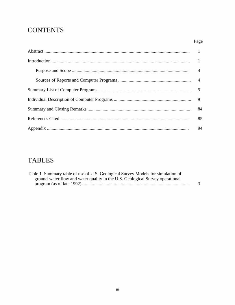
CONTENTS
Page
Abstract .............................................................................................................................. 1
Introduction ........................................................................................................................ 1
Purpose and Scope ...................................................................................................... 4
Sources of Reports and Computer Programs ............................................................... 4
Summary List of Computer Programs ................................................................................ 5
Individual Description of Computer Programs ................................................................... 9
Summary and Closing Remarks ......................................................................................... 84
References Cited ................................................................................................................ 85
Appendix ........................................................................................................................... 94
TABLES
Table 1. Summary table of use of U.S. Geological Survey Models for simulation ofground-water flow and water quality in the U.S. Geological Survey operationalprogram (as of late 1992) ............................................................................................. 3

iv
On the cover: Background – The experimental apparatus of Darcy (1856), used in the empirical
determination of the basis momentum balance equation for ground water, known as Darcy’s law.
Foreground – A two-dimensional flow net (DaCosta and Bennett, 1960). Artwork by Joan Rubin and Leslie Robinson

ons to ams werk ected the y are ction
SUMMARY OF SELECTED COMPUTER PROGRAMS PRODUCED BY THE U.S. GEOLOGICAL SURVEY FOR SIMULATION OF
GROUND-WATER FLOW AND QUALITY, 1994
By
Charles A. Appel and Thomas E. Reilly
ABSTRACT
A summary list of computer models that simulate ground-water flow and quality is presented. The list contains a brief description of each model program, its numerical features, a qualitative expression of the number of past applications, the reference for the report documenting the pro-gram, and where to obtain a copy. Reports included in the list have been published or developed by the U.S. Geological Survey, and contain listings of the computer programs, although in a few cases, the program is so long that a listing was not included in the report, but a copy of the program is available on request.
INTRODUCTION
Numerical models provide a powerful aid in understanding and assessing ground-water systems. The U.S. Geological Survey (USGS) has contributed significantly to the development and use of models for the analysis of ground-water problems. Two reports had previously documented the status of ground-water modeling in the USGS, Appel and Bredehoeft (1976) and Appel and Reilly (1988). Because developments in the field have taken place since that time, additional computer programs have been published. This report gives information on selected computer programs published or developed by the USGS or by the USGS in cooperation with Federal, State, and local agencies for modeling flow, quality, and solute or heat transport in ground-water systems. The information for each program includes the reference, a brief description of the field conditions that the program can simulate, the numerical approximation procedures used, an indication of the extent of past field applications of the program by USGS personnel, and where to obtain copies of the report and, in some cases, the computer code.
The list of programs is organized by general modeling category. Information on each program is separated by one solid horizontal line. In many cases a program is based on or related to another program. The parent program is listed first and followed by the related programs. Three solid lines mark the end of the list of those programs related to a parent computer program. In a few cases, however, a program listed under one category was derived from a program in another category; for example, some of the programs listed in the “Freshwater-Saltwater” category are modificatiground-water flow programs described in the category “Flow-Saturated.” Also, some progrcould be included under other categories; for example, the programs by Grove and Stollen(1984) and Lewis, Voss, and Rubin (1986) are models for the transport of fluids that are affby physical and chemical processes. Both of those programs could have been included in“Chemical Mass Transfer” category instead of the category of “Solute Transport” in which thecontained in this report. Although several flow models that account for surface-water intera
1

finitely a than zone.
rein. lized
ped in cts of eports m have g that a ement h the
odel t time es or ause of rojects rt are ng
are listed as having been derived from some parent flow model, we have listed the coupled ground- and surface-water flow model of Swain and Wexler (1993) separately even through it represents a coupling of the ground-water flow model of McDonald and Harbaugh (1988) and a surface-water flow model of Schaffranek, Baltzer, and Goldberg (1981). This choice was made to bring attention to the fact that it is the only case in which the surface-water formulation is based on a comprehensive set of unsteady flow equations, which are subject only to the limitations inherent in a one-dimensional formulation of streamflow. The intent of these examples is to indicate that a potential user should thoroughly evaluate the programs in all related categories to choose the most appropriate numerical tool. The category titles are generalized and are not intended to be all-inclusive.
Depending on the nature of the problem, more than one computer program may apply. In some cases, the choice of program may reflect more the individual’s familiarity with a particular approach than the superiority of the approach. In other cases, the choice of program may dereflect the level of approximation required; for example, if field data indicate a thick zone ofbrackish water that separates strictly fresh water from strictly salt water, then the choice of program that assumes the zone is an interface may result in a lesser level of approximationwould a solute-transport program that includes consideration of the density variations in the
Many computer programs for the simulation of ground-water flow and quality are listed heSome of these programs are listed for historical reasons or because they represent speciaaspects of either physics or chemistry. Additionally, many areas of ground-water flow and chemistry are the subjects of multiple investigations, in which related programs are develoan attempt to refine and (or) perfect the methods currently available; therefore, some aspeground water can be simulated by more than one model listed in this report. Although the rthat document the programs have been reviewed and approved, not all parts of every progranecessarily been thoroughly tested, and a user bears the ultimate responsibility for assurinprogram does, in fact, what is claimed. Confidence in a program increases with good agrebetween program results and known solutions to problems closely related to those for whicprogram is intended to solve.
As an indication of models that are currently “popular,” a poll was made in late 1992 of musage in the U.S. Geological Survey’s operational program. The models being used at thaare listed in table1. This listing provides general information on usage. However, new codspecialty codes may not be included (or may be under represented) in this table simply becthe available utility of the codes at the start of these projects and the scope of the current pbeing undertaken. Associated with many of the computer programs discussed in this repoacronyms. Appendix 1 gives a list of those acronyms and the full name of the correspondiprogram and the appropriate reference(s).
2

TABLE 1. Summary table of use of U.S. Geological Survey Models for simulation of ground-water flow and water quality in the U.S. Geological Survey operational program (as of late 1992)______________________________________________________________________________
Number of ProjectsModel Name Using the Model
______________________________________________________________________________
AQUIFEM-SALT (Voss, 1984b) ................................................................................4AX (Rutledge, 1991)...................................................................................................1BALANCE (Parkhurst and others, 1982) .................................................................10HST3D (Kipp, 1987) ..................................................................................................8INTERCOMP (INTERCOMP, 1976; INTERA, 1979) ..............................................2MOC (Konikow and Bredehoeft, 1978; Goode and Konikow, 1989) ........................8MODFE (Torak, 1993a, b; Cooley, 1992) ..................................................................4MODFLOW (McDonald and Harbaugh, 1988)......................................................165MODFLOWP (Hill, 1992)..........................................................................................8MODPATH (Pollock, 1989)......................................................................................54NETPATH (Plummer and others, 1991) ...................................................................29PHREEQE (Parkhurst and others, 1980; revised, 1990) ..........................................36PHRQPITZ (Plummer and others, 1988) ...................................................................2SHARP (Essaid, 1990) ...............................................................................................8SOLMINEQ (Kharaka and others, 1988) ...................................................................3SUTRA (Voss, 1984a) ..............................................................................................12TRACY (Dunlap and others, 1984) ............................................................................2Trescott-3D (Trescott, 1975).......................................................................................1Variable Density Flow (Kuiper, 1985)........................................................................1VS2D (Lappala and others, 1987) ..............................................................................8WATEQF (Plummer and others, 1976; revised, 1984) .............................................11WATEQ4F (Ball and Nordstrom, 1991) ...................................................................20
______________________________________________________________________________
3

Purpose and Scope
This report makes available a moderately comprehensive list of computer programs that have been produced by the U.S. Geological Survey for simulation of ground-water flow and quality. The main criterion used in compiling the list is that the program must be documented in a published report that includes a listing of the computer program, although in a few cases, the program is so long that a listing was not included in the report, but a copy of the program is available on request.
Sources of Reports and Computer Programs
For those reports not available from a cooperating State agency, an indication is given from which of the following Federal sources the report and computer program can be obtained:
U.S. Geological SurveyNWIS Program Office437 National CenterReston, VA 22092(703) 648-5695
NTIS, U.S. Department of Commerce5285 Port Royal RoadSpringfield, VA 22161703) 487-4650
U.S. Geological Survey Open-File Reports and Water-Resources Investigations Reports, can be purchased from:
USGS ESIC--Open-File Report SectionBox 25286, MS 517Denver Federal CenterDenver, CO 80225-0046(303) 236-7476
U.S. Geological Survey Water-Supply Papers, Professional Papers, Bulletins, Circulars, and Techniques of Water-Resources Investigations, can be purchased from:
USGS Map DistributionBox 25286, MS 306Denver Federal CenterDenver, CO 80225(303) 236-7477
4

0
0
11
4
17
2122
2
3
3
4
SUMMARY LIST OF COMPUTER PROGRAMS
Page
Flow—Saturated:
Two-dimensional finite difference (Trescott, Pinder, and Larson, 1976) ............. 9Direct matrix-solver using D4 node ordering (Larson, 1978) ......................... 1Conjugate-gradient matrix solver (Manteuffel, Grove, and
Konikow, 1983) .......................................................................................... 1Approximate surface-water interaction (Ozbilgin and Dickerman, 1984) ....... 10Head-dependent flux procedure along model boundary (Hutchinson,
Johnson, and Gerhart, 1981) .....................................................................Two-dimensional finite element, steady state (Kuniansky, 1990) ....................... 12Two-dimensional finite element Galerkin (including river accounting
procedure) (Dunlap, Lindgren, and Carr, 1984)............................................. 12Two-dimensional finite element (kinematic equation representing
river flows) (Glover, 1988) ............................................................................. 13Two-dimensional finite element (including transient leakage effects)
(Cooley, 1992; Torak, 1993a, b) ...................................................................... 1Cylindrical coordinates (Finite-element Galerkin) (Reilly, 1984) ..................... 16
Pre- and post-processor (Pucci and Pope, 1987) ..............................................Axisymmetric finite difference (well bore/aquifer) (Rutledge, 1991)................. 17Two-aquifer system (Finite-element Galerkin) (Mallory, 1979)......................... 18Quasi-three dimensional aquifer system (Finite difference) (Weeks, 1978) ..... 19Three-dimensional finite difference (Bredehoeft, 1992) ...................................... 20Three-dimensional finite difference (Trescott, l975; Trescott and
Larson, 1976) ....................................................................................................Include head-dependent sources/sinks (Torak, 1982).......................................Include conversion from confined to unconfined flow, recharge to any
layer, and other modifications (Helgesen, Larson, and Razem, 1982) ..... 2Include transient leakage in confining layers and added program to compute
sensitivity of parameter changes (Torak and Whiteman, 1982) ............... 2Include transient leakage from confining layers, change method of
handling confining-bed and aquifer pinchouts, reduce computermemory needed (Leahy, 1982) ................................................................... 2
Approximate land subsidence induced by pumping (Meyer and Carr, 1979) .................................................................................................. 2
Three-dimensional finite difference (include transient leakage from confining layers, “cube” input capability) (Posson and others, 1980)......... 24
Improve treatment of boundaries, revise code to run on CRAY-1 computer(Hearne, 1982) ............................................................................................ 25
Three-dimensional finite-difference (McDonald and Harbaugh, l988)................ 26Preconditioned conjugate gradient matrix solvers (Kuiper, 1987) ................... 27Statistical processor (Scott, 1990) .................................................................... 27Read and write geographical information system (GIS) files (Orzol and
McGrath, 1992)......................................................................................... 28
5

1
4
6
6
47
7
Page
Calculation of water budgets (Harbaugh, 1990) ............................................... 28Aquifer compaction (Leake and Prudic, 1991)................................................. 29River routing and accounting (Miller, 1988) .................................................... 29Handling narrow canyons and faults and layer pinchouts (Hansen, 1993)....... 30Stream-aquifer relations (Prudic, 1989)............................................................ 30Calculation of pathlines (Pollock, 1989, 1990) ................................................ 31Preconditioned conjugate-gradient matrix solver 2 (Hill, 1990) ...................... 31Parameter estimation (Hill, 1992)..................................................................... 32Generalized finite-difference formulation (Harbaugh, 1992)........................... 33Cylindrical flow to a well (Reilly and Harbaugh, 1993b) ................................ 34Alternative of different interblock transmissivity conceptualizations
(Goode and Appel, 1992).......................................................................... 34Simulate horizontal-flow barriers (Hsieh and Freckleton, 1993) ..................... 35Rewetting dry cells (McDonald, and others, 1992) ......................................... 35Simulate transient leakage from confining units (Leake, Leahy, and
Navoy, in press) .......................................................................................... 36Two-dimensional--parameter estimation (Cooley and Naff, 1990) .................... 37Coupled ground-water and surface-water flow (Swain and Wexler, 1993) ....... 38
Flexibility in representing surface water system (Swain, 1993)....................... 39Soil moisture accounting program coupled to a two-dimensional
unconfined-confined aquifer system (Reed, Bedinger, and Terry, 1976) ..... 39
Flow—Variably saturated:
Two-dimensional (Lappala, Healy, and Weeks, 1987) .......................................... 4Simulation of trickle irrigation (Healy, 1987) .................................................. 42
Two-dimensional diffusion (Ishii, Healy, and Striegl, 1989) ................................ 42
Solute transport—Saturated:
One-dimensional finite-difference method (equilibrium-controlled sorptionand irreversible-rate reaction) (Grove and Stollenwerk, 1984) ................... 44
Two-dimensional method of characteristics (advective transport, dispersion, and decay and equilibrium-controlled sorption or ion exchange) Konikow and Bredehoeft, 1978; Goode and Konikow, 1989) ........................ 4Front tracking (advective transport only) (Garabedian and
Konikow, 1983) .......................................................................................... 4Two constituent solute transport, including density-dependent flow
Stanford and Konikow, 1985)................................................................... 4Two-dimensional finite-element Galerkin method (advective transport,
dispersion, sorption, ion exchange, equilibrium chemistry) (Lewis, Voss, and Rubin, 1986)....................................................................................
Dual porosity flow and transport (nonreactive advective transport anddispersion in fractures, diffusion between fractures and rock)(Glover, 1987).................................................................................................. 4
6

0
53
8
68
70
Page
Solute transport—Variably saturated:
Two-dimensional (Healy, 1990)............................................................................. 49
Solute and heat transport—Saturated:
Three-dimensional finite-difference method (INTERCOMP, 1976) .................. 50Include water table, recharge, equilibrium controlled adsorption andirreversible-rate reaction (INTERA, 1979)....................................................... 5
Three-dimensional finite-difference method (Kipp, l987) .................................. 51
Flow—Saturated freshwater/saltwater:
Two-dimensional areal (Sharp interface) (Mercer, Larson, and Faust, 1980) .....................................................................................................
Two-dimensional areal (Sharp interface) (Voss, 1984b)..................................... 54Three-dimensional (Sharp interface) (Guswa and LeBlanc, 1985) ..................... 55Three-dimensional (Sharp interface) (Sapik, 1988) ............................................ 55Three-dimensional (Sharp interface) (Essaid, 1990) ........................................... 56Three-dimensional (Variable density) (Weiss, 1982) .......................................... 57Three-dimensional (Variable density) (Kuiper, 1985)......................................... 58Three-dimensional (Variable density and multiaquifer wells) (Kontis and
Mandle, 1988) .................................................................................................. 5
Heat transport:
Two-dimensional single-and two-phase (Faust and Mercer, 1977)...................... 60Two-dimensional single phase (liquid) (Mercer and Pinder, 1975) ..................... 60Three-dimensional (single phase-liquid) (Reed, 1985) ........................................ 61Three-dimensional (multiphase) (Hayba and Ingebritsen, in press)..................... 62
Solute or heat transport—Saturated and unsaturated:
Two-dimensional finite-element Galerkin method (fluid-density dependent advective transport, dispersion, equilibrium controlled adsorption, zero-order production or decay) (Voss, 1984a) ............................................ 64
Aquifer management:
Two-dimensional saturated flow (Lefkoff and Gorelick, 1987)........................... 66Three-dimensional saturated flow (Puig and Rolon-Collazo, in press) ............... 67
Chemical mass balance:
Mass balance and electron conservation (Any elements, specified phases)(Parkhurst, Plummer, and Thorstenson, 1982) ................................................
Characterization of natural waters (Bodine and Jones, 1986) ............................ 69Mass balance reaction models satisfying specified constraints (Plummer,
Prestemon, and Parkhurst, 1991) .....................................................................
7

0
812
Page
Aqueous speciation:
Speciation of major and some minor elements in 0-100 oC temperature range (Truesdell and Jones, 1973, 1974) ................................................................... 72FORTRAN IV version (Plummer, Jones, and Truesdell, 1976;
revised, 1984).............................................................................................. 73Expands thermodynamic data base and adds trace elements (Ball,
Nordstrom, and Jenne, 1980) ...................................................................... 74Adds uranium (Ball, Jenne, and Cantrell, 1981)............................................... 75Expanded personal computer, FORTRAN version of WATEQ4F (Ball and
Nordstrom, 1991)........................................................................................ 75
Chemical mass transfer:
System CaO-MgO-Na2O-K2O-CO2-H2SO4-HCl-H2O (Plummer, Parkhurst,and Kosiur, 1975)............................................................................................. 77
Mineral and water/gas interactions at low temperatures (Subject tothermodynamic constraints—any elements, specified phases),(Parkhurst, Thorstenson, and Plummer, 1980; revised, 1990)......................... 78Interactive program for forming data input (Fleming and Plummer, 1983) ..... 79Incorporate Pitzer’s equations for brines (Plummer and others, 1988) ............ 8
Speciation of major and many minor elements with mineral and waterinteractions in 0-350 oC temperature range (Kharaka and Barnes, 1973) .. 81Updated program (Kharaka and others, 1988)..................................................Processor to create and modify input (DeBraal and Kharaka, 1989) ............... 8
Nonideal solid-solution aqueous-solution reactions (Glynn, 1991a)................... 83
8

uifer of chap.
aped
ncipal st be s well
ining iration s can
. m is lution
and and as
ional d as ains
ort
______
INDIVIDUAL DESCRIPTIONS OF COMPUTER PROGRAMS
FLOW—SATURATED
Two-Dimensional Finite Difference
Program Documentation:
Trescott, P.C., Pinder, G.F., and Larson, S.P., 1976, Finite-difference model for aqsimulation in two dimensions with results of numerical experiments: TechniquesWater-Resources Investigations of the United States Geological Survey, book 7, C1, 116 p.
Description:
This model simulates steady and nonsteady ground-water flow in an irregularly shaquifer that can be a confined or unconfined aquifer or both. The transmissive properties of the aquifer may be heterogeneous and anisotropic, although the pridirections of anisotropy must be aligned with the grid and the anisotropy ratio muconstant, and the storage coefficient may be heterogeneous. The model simulatedischarge; recharge that can differ spatially, but not with time; leakage from a confbed or streambed in which the effects of storage are considered; and evapotranspas a linear function of depth to water. Specified head and specified flux boundariebe simulated.
Numerical features:
The grid is block centered and rectangular with variable spacing in each directionFinite difference numerical approximations are used. The resulting matrix problesolved by an iterative procedure; the user has a choice of selecting one of three soalgorithms: line successive overrelaxation, iterative alternating direction implicit,the strongly implicit procedure. Mass balances are computed for each time step a cumulative volume of water from each source and each type of discharge.
Past applications:
Up to a few years ago, this was one of the most-used flow models for two-dimensproblems. See McDonald and Harbaugh (1988), which is one of the reports liste“Flow-Saturated--Three-dimensional finite difference,” for a newer code that contmost of the capabilities of this program.
Availability:
Report is available from the USGS Map Distribution. Computer program and repare available from NWIS.
________________________________________________________________________
9

Related program:
Larson, S.P., 1978, Direct solution algorithm for the two-dimensional ground-water flow model: U.S. Geological Survey Open-File Report 79-202, 22 p.
Most significant change to original program:
A direct-matrix-solver program that assumes the D4 (alternating diagonal) node-ordering scheme is presented. For moderate-sized grids, this solver can be computationally more efficient than iterative matrix methods.
Past applications:
Many.
Availability:
Report is available from the USGS ESIC--Open-File Report Section. Computer program and report are available from NWIS.
______________________________________________________________________________
Related program:
Manteuffel, T.A., Grove, D.B., and Konikow, L.F., 1983, Application of the conjugate-gradient method to ground-water models: U.S. Geological Survey Water-Resources Investigations Report 83-4009, 24 p.
Most significant change to original program:
A conjugate-gradient matrix solution procedure is presented for the two-dimensional ground-water flow problem. Application to a field problem of this method as compared with the iterative alternating direction implicit procedure (IADIP) and the strongly implicit procedure (SIP) methods showed the conjugate gradient method to compare favorably with IADIP but less satisfactorily with SIP. The main advantage of the conjugate gradient method is that it does not require the use of iteration parameters.
Past applications:
Few.
Availability:
Report is available from the USGS ESIC--Open-File Report Section.______________________________________________________________________________
Related program:
Ozbilgin, M.M., and Dickerman, D.C., 1984, A modification of the finite-difference model for simulation of two-dimensional ground-water flow to include surface-ground water relationships: U.S. Geological Survey Water-Resources Investigations Report 83-4251, 98 p.
10
l grid, e e strip ies of
__________________
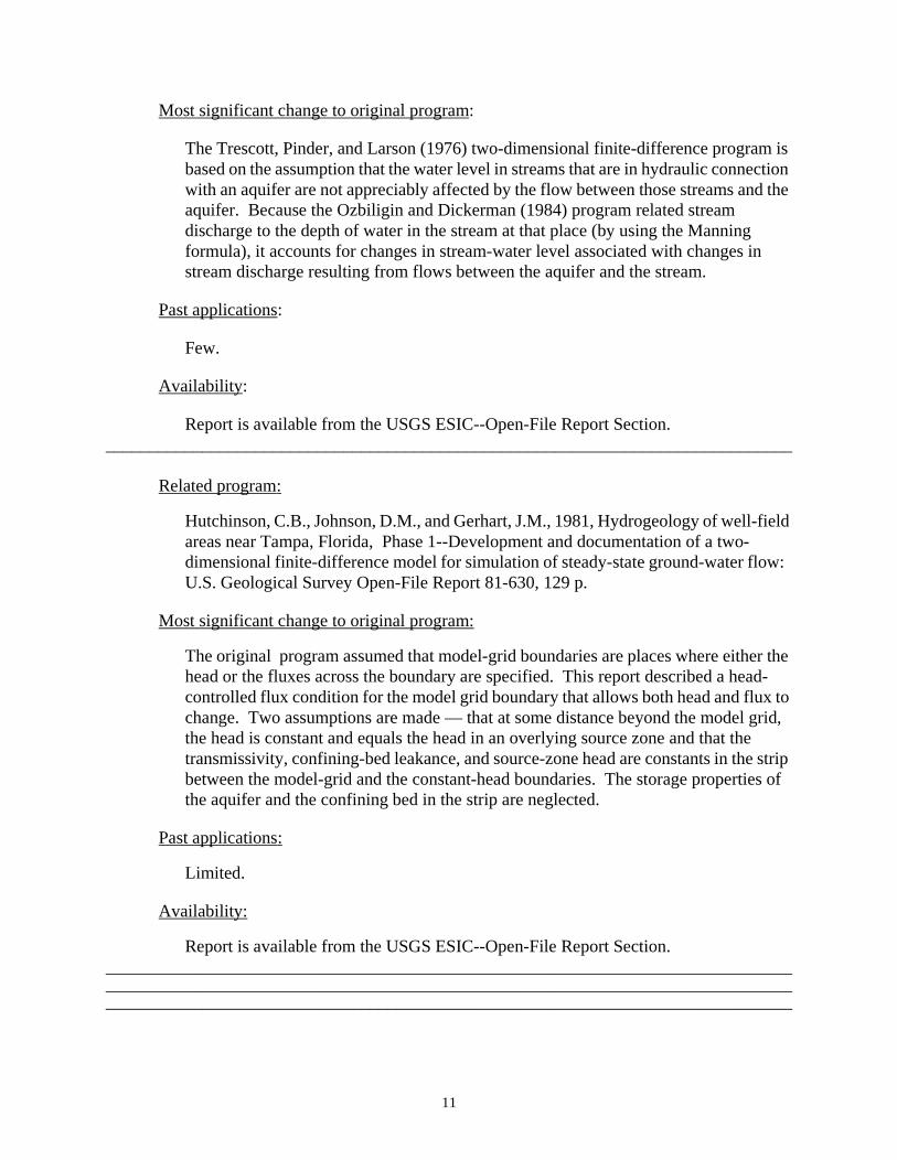
Most significant change to original program:
The Trescott, Pinder, and Larson (1976) two-dimensional finite-difference program is based on the assumption that the water level in streams that are in hydraulic connection with an aquifer are not appreciably affected by the flow between those streams and the aquifer. Because the Ozbiligin and Dickerman (1984) program related stream discharge to the depth of water in the stream at that place (by using the Manning formula), it accounts for changes in stream-water level associated with changes in stream discharge resulting from flows between the aquifer and the stream.
Past applications:
Few.
Availability:
Report is available from the USGS ESIC--Open-File Report Section.______________________________________________________________________________
Related program:
Hutchinson, C.B., Johnson, D.M., and Gerhart, J.M., 1981, Hydrogeology of well-field areas near Tampa, Florida, Phase 1--Development and documentation of a two-dimensional finite-difference model for simulation of steady-state ground-water flow: U.S. Geological Survey Open-File Report 81-630, 129 p.
Most significant change to original program:
The original program assumed that model-grid boundaries are places where either the head or the fluxes across the boundary are specified. This report described a head-controlled flux condition for the model grid boundary that allows both head and flux to change. Two assumptions are made — that at some distance beyond the modethe head is constant and equals the head in an overlying source zone and that thtransmissivity, confining-bed leakance, and source-zone head are constants in thbetween the model-grid and the constant-head boundaries. The storage propertthe aquifer and the confining bed in the strip are neglected.
Past applications:
Limited.
Availability:
Report is available from the USGS ESIC--Open-File Report Section.________________________________________________________________________________________________________________________________________________________________________________________________________________________
11

Two-Dimensional Finite Element
Program Documentation:
Kuniansky, E.L., 1990, A finite-element model for simulation of two-dimensional steady-state ground-water flow in confined aquifers: U.S. Geological Survey Open-File Report 90-187, 77 p.
Description:
This report described a finite-element model that can be used to simulate two-dimensional steady-state ground-water flow in either isotropic or anisotropic aquifers. The principal axes of anisotropy can vary in direction over the modeled area, and the transmissivity can vary spatially, but not with changes in head. Constant head, constant flux, and head-dependent flux boundary conditions can be simulated.
Numerical features:
The computer program is based on the Galerkin finite-element technique and it uses triangular elements.
Past applications:
Limited.
Availability:
Report is available from the USGS ESIC--Open-File Report Section.__________________________________________________________________________________________________________________________________________________________________________________________________________________________________________
Two-Dimensional Finite-Element Galerkin
Program Documentation:
Dunlap, L.E., Lindgren, R.J., and Carr, J.E., 1984, Projected effects of ground-water withdrawals in the Arkansas River Valley, 1980-99, Hamilton and Kearny Counties, southwestern Kansas: U.S. Geological Survey Water-Resources Investigations Report 84-4082, 168 p. (Pages 27 to 168 contain documentation for the program developed by J. V. Tracy.)
Description:
This model simulates steady and nonsteady two-dimensional ground-water flow in an irregularly shaped confined or unconfined aquifer. The transmissive and storage properties of the aquifer may be heterogeneous. The model accounts for gains and losses from the river flow in each reach based on the incoming river and tributary flows and the gain from or loss to the aquifer in the reach. With an estimate of river discharge,
12

as or the med blem puted
the
__________________
f ons
y’s ound-nd
eam- zones te e, and
the river stage is computed for each reach by using an input stage-discharge relation given for each reach. The river/aquifer gains and losses are calculated as a function of streambed area, riverbed leakance values, and the head gradient between the river and the aquifer. Evapotranspiration from ground water is estimated by using monthly values of precipitation, applied water rate, evapotranspiration demand, the moisture capacity of the soil zone, and depth of root zone. Well discharges can vary monthly. Specified flux and specified head boundaries can be simulated.
Numerical features:
A “regular” finite-element grid is used in the simulation. A “regular” grid is defineda region subdivided by a given number of columns that do not have to be parallel same length but that have an equal number of elements. The effect is of a deforrectangular grid. Applying the Galerkin method results in an associated matrix prothat is solved by using a direct method. Mass balances from all sources are comfor each time step and as a cumulative volume for each source from the start of simulation.
Past applications:
Several field problems.
Availability:
Report is available from the USGS ESIC--Open-File Report Section. Computer program and report are available from NWIS.
________________________________________________________________________________________________________________________________________________________________________________________________________________________
Two-Dimensional Finite Element (kinematic equation representing river flows)
Program Documentation:
Glover, K.C., 1988, A finite-element model for simulating hydraulic interchange osurface and ground water: U.S. Geological Survey Water-Resources InvestigatiReport 86-4319, 90 p.
Description:
This model couples the equation of two-dimensional ground-water flow with the kinematic equation approximation for one-dimensional open-channel flow. Darclaw for vertical flow through a semipermeable streambed is used to couple the grwater flow and streamflow equations. The transmissive and storage properties adistributed recharge/discharge of the aquifer can vary by element, as can the strchannel properties. Elements can be grouped together into user-defined propertyfor ease of varying the magnitudes of those properties. The program can simulaperched streams, streamflow diversions, springs, recharge from irrigated acreagevapotranspiration.
13

s: chap.
ues
ns,
d on w in
Numerical features:
Triangular elements are used to approximate the aquifer, and one-dimensional linear elements located along the sides of the aquifer elements are used to approximate the stream network. The stream depth, stream velocity, and aquifer head are approximated throughout the stream/aquifer system as varying linearly within elements and are continuous between adjacent elements. The program assumes that the changes in hydraulic head are small and that the aquifer transmissivity does not change. Modifications to the program are outlined for the case where the aquifer transmissivity changes with hydraulic head.
Past applications:
Few.
Availability:
Report is available from the USGS ESIC--Open-File Report Section.__________________________________________________________________________________________________________________________________________________________________________________________________________________________________________
Two-Dimensional Finite Element (including transient leakage effects)
Program Documentation:
Torak, L.J., 1993a, Model description and user’s manual; Part 1 of A MODular Finite-Element model (MODFE) for areal and axisymmetric ground-water-flow problemU.S. Geological Survey Techniques of Water-Resources Investigations, book 6, A3, 136 p.
Cooley, R.L., 1992, Derivation of finite-element equations and comparisons withanalytical solutions; Part 2 of A MODular Finite-Element model (MODFE) for areal and axisymmetric ground-water-flow problems: U.S. Geological Survey Techniqof Water-Resources Investigations, book 6, chap. A4, 108 p.
Torak, L.J., 1993b, Design philosophy and programming details; Part 3 of A MODular Finite-Element model (MODFE) for areal and axisymmetric ground-water-flow problems: U.S. Geological Survey Techniques of Water-Resources Investigatiobook 6, chap. A5, 243 p.
Description:
MODFE was developed to provide solutions to ground-water flow problems basethe governing equations that describe two-dimensional and axisymmetric-radial floporous media. The documentation is divided into three parts.
14
ilities o ata water ines
o
he ations
isons
cture e s with
the he ts of rror fined
the
ime Linear ts. an be he
ns, thin lly uted d-
Part 1 is the user’s manual in which the hydrologic features and simulation capabof MODFE are described. Descriptions are given for preparing hydrologic data tcharacterize aquifer properties and boundary conditions by zone. Examples of dinput and model output are provided to demonstrate the different types of ground-problems that are solved by using the simulation capabilities of MODFE. Guidelfor designing the finite-element mesh and for node numbering and determining bandwidths are given to instruct users in the appropriate application of MODFE tground-water problems.
In Part 2, the finite-element equations are derived by minimizing a functional of tdifference between the true and approximate hydraulic head, which produces equthat are equivalent to those obtained by either classical variational or Galerkin techniques. Spatial finite elements are triangular with linear basis functions, andtemporal finite elements are one dimensional with linear basis functions. Comparof finite-element solutions with analytical solutions are given for five example problems.
Part 3 contains descriptions of subroutines, programming details and program strudiagrams. Descriptions of subroutines that execute the computational steps of thmodular-program structure are given in tables that cross-reference the subroutineparticular versions of MODFE. Programming details of linear and nonlinear hydrologic terms are provided. Structure diagrams for the main programs show order in which subroutines are executed for each version and illustrate some of tlinear and nonlinear versions of MODFE that are possible. Computational aspecchanging stresses and boundary conditions with time and of mass balance and eterms are given for each hydrologic feature. Program variables are listed and deaccording to their occurrence in the main programs and subroutines. Listings ofmain programs and subroutines are given.
Numerical features:
Aquifer geometry, flow boundaries, and variations in hydraulic properties are represented by triangular elements or element sides in a finite-element mesh. Tvariations in hydraulic response are represented by one-dimensional elements. coordinate functions are used to approximate the head distribution within elemenThe finite-element matrix equations are solved by using either a direct symmetricDoolittle method of triangular decomposition or an iterative method that uses themodified, incomplete Cholesky, conjugate-gradient method. The direct method cefficient for small- to medium-sized problems (less than about 500 nodes), and titerative method generally is more efficient for larger-sized problems.
Simulation capabilities and uses of MODFE are transient or steady-state conditiononhomogeneous and anisotropic flow where directions of anisotropy change withe model region; vertical leakage from a semiconfining layer that contains lateranonhomogeneous properties and elastic storage effects; point and areally distribsources and sinks; specified head (Dirichlet), specified flow (Neumann), and hea
15

dependent (Cauchy-type) boundary conditions; vertical cross-section and axisymmetric cylindrical flow; confined and unconfined (water-table) conditions; partial drying and resaturation of a water-table aquifer; conversion between confined- and unconfined-aquifer conditions; and nonlinear head-dependent fluxes (for simulating line, point, or areally distributed sources and sinks). Aquifer stresses and boundary conditions can be changed on a time-step basis, or a stress-period basis or both. Hydraulic properties and boundary conditions can be input by zone.
Past applications:
This is a new program that has been used in a few field studies.
Availability:
Reports are available from the USGS Map Distribution. Computer program and reports are available from NWIS.
__________________________________________________________________________________________________________________________________________________________________________________________________________________________________________
Cylindrical Coordinates
Program Documentation:
Reilly, T.E., 1984, A Galerkin finite-element flow model to predict the transient response of a radially symmetric aquifer: U.S. Geological Survey Water-Supply Paper 2198, 33 p.
Description:
This computer program was developed to evaluate radial flow of ground water at a pumping well, a recharge basin, or an injection well. It is capable of simulating anisotropic, inhomogenous, confined, or pseudounconfined (constant saturated thickness) conditions.
Numerical features:
The program is based on the Galerkin finite-element technique. It uses linear triangular elements and a backwards finite difference in time.
Past applications:
Several.
Availability:
Report is available from the USGS Map Distribution. Computer program and report are available from NWIS.
______________________________________________________________________________
16

Related program:
Pucci, A.A., Jr., and Pope, D.A., 1987, Preprocessor and postprocessor computer programs for a radial-flow, finite-element model: U.S. Geological Survey Open-File Report 87-680, 69 p.
Most significant change to original program:
This program serves as a preprocessor by: generating a triangular finite-element mesh from minimal data input, producing graphical displays and tabulations of data for the mesh, and preparing an input data file. The postprocessor has the ability to produce graphical output for simulation and field results and to generate statistics for comparing the simulation results with observed data.
Past applications:
Limited.
Availability:
Report is available from the USGS ESIC--Open-File Report Section.
__________________________________________________________________________________________________________________________________________________________________________________________________________________________________________
Axisymmetric Finite-Difference (well bore/aquifer)
Program Documentation:
Rutledge, A.T., 1991, An axisymmetric finite-difference flow model to simulate drawdown in and around a pumped well: U.S. Geological Survey Water-Resources Investigations Report 90-4098, 33 p.
Description:
This computer program was developed to simulate drawdown in and around a pumped well. It provides a tool that is useful for analyzing some aquifer test data that are complicated by features not handled by analytical methods. Aquifer properties that can be simulated include confined (leaky or nonleaky) conditions, unconfined conditions, vertical-horizontal anisotropy, and vertical variation in hydraulic conductivity and specific storage. The model requires horizontal uniformity of hydraulic conductivity, specific yield, and specific storage. Well properties that can be simulated include well-casing storage, hydraulic head loss across the well screen, and hydraulic head variation along the length of the well bore that results from pipe-flow friction and nonuniform velocity. The program allows for partial well penetration and for multiple screened intervals.
17

Numerical features:
The program is based on the finite-difference technique. Because the time derivative approximation used is the forward-difference (explicit) in time, an upper limit on the time-step length is needed to assure numerical stability. The program allows an early time-step size and a larger later time-step size.
Past applications:
Limited.
Availability:
Report is available from the USGS ESIC--Open-File Report Section.__________________________________________________________________________________________________________________________________________________________________________________________________________________________________________
Two-Aquifer System
Program Documentation:
Mallory, M.J., 1979, Documentation of a finite-element two-layer model for simulation of ground-water flow: U.S. Geological Survey Water-Resources Investigations Report 79-18, 347 p.
Description:
Theoretical development of the model represented by this program is from Durbin (1978). The program simulates steady and nonsteady ground-water flow in an irregularly shaped two-aquifer system. The areal extent of the two aquifers does not have to be coincident. The transmissive and storage properties of the aquifer can differ spatially but are assumed to be isotropic. Discharge and recharge can be varied spatially and with time. Evapotranspiration is treated as a linear function of depth to water. The vertical hydraulic conductivity of the confining layer is assumed to be a constant, its thickness can differ spatially, and the changes in confining layer storage are assumed to be negligible.
Numerical features:
The program uses the Galerkin finite-element method and approximates the time derivative by backwards finite-difference formulation. The region to be modeled is subdivided into triangles, and the head is assumed to vary linearly in any one triangle. The associated matrix problem is solved by using the PSOR (point iterative successive over-relaxation method).
Past applications:
A few field applications.
18

__________________
ces
a and stem fining f each
ad
lock-
atrix licit m as a
lar the lying ified of
Availability:
Report is available from NTIS (PB–80–140–932).________________________________________________________________________________________________________________________________________________________________________________________________________________________
Quasi-Three-Dimensional Aquifer System (Finite Difference)
Program Documentation:
Weeks, J.B., 1978, Digital model of ground-water flow in the Piceance Basin, RioBlanco and Garfield Counties, Colorado: U.S. Geological Survey Water-ResourInvestigations 78-46, 108 p.
Description:
The computer program capability is “quasi-three-dimensional” in that it simulatesthree-dimensional multiaquifer system by assuming horizontal flow in the aquifersvertical flow through the confining layers that separate the aquifers. The programsimulates steady and nonsteady ground-water flow in an irregularly shaped flow sythat consists of aquifer layers and confining layers. Changes in storage in the conlayers are assumed to be negligible. The transmissivity and storage coefficient oaquifer layer and the confining layer leakance values can differ spatially. Uniformrecharge to each layer and distributed discharge can be simulated. Specified heboundaries can be simulated in the uppermost aquifer.
Numerical features:
The planar area of the irregularly shaped flow region is divided into a rectangular bcentered grid that permits variable grid spacing. Finite-difference numerical approximations reduce the equations of ground-water flow in each aquifer to a mproblem that can be solved by using IADIP (the iterative alternating-direction impprocedure). The computational procedure essentially is to treat the aquifer systesequence of two-dimensional flow models coupled by terms that represent flow (leakage) through intervening confining beds. The leakage at a node in a particulayer is based on, among other things, the difference in head in the layer during current iteration and the most recently computed heads for the nodes in the overand underlying layers vertically in line with the subject node. Outflows to the spechead boundaries are computed for each time period and as a cumulative volumewater.
Past applications:
Many.
19

__________________
ter port
s run aries
with torage umed the
rties ns plicit stem
Remarks:
This program is a revision and adaptation for the Piceance Basin of a program developed by J. D. Bredehoeft in 1969 and described in Bredehoeft and Pinder (1970); the latter program was used widely before about 1980. See McDonald and Harbaugh (1988) for a newer code that has more capabilities.
Availability:
Report is available from NTIS (PB–284–341).________________________________________________________________________________________________________________________________________________________________________________________________________________________
Three-Dimensional Finite-Difference
Program Documentation:
Bredehoeft, J.D., 1992, Microcomputer codes for simulating transient ground-waflow—In two and three space dimensions: U.S. Geological Survey Open-File Re90-559, 73 p., diskette in pocket.
Description:
This report is the documentation for a code for solving two- and quasi-three-dimensional formulations of the general ground-water flow equation. The code iwritten in FORTRAN 77 and was developed to be a simple basic code that couldon a variety of small computer systems. Specified head and specified flux boundcan be simulated. The transmissivity is assumed to be isotropic and not changehead, but it can vary spatially. One value is assumed to be representative of the scoefficient of all aquifers, and the effects of storage in the confining layers are assto be negligible. The leakance values (vertical hydraulic conductivity divided by thickness of the leaky confining layer) can vary spatially for each confining layer.Recharge/discharge can be simulated and can vary spatially.
Numerical features:
The flow region is considered to be divided into blocks in which the medium propeare assumed to be uniform. Block-centered finite-difference numerical formulatioare used. The associated matrix problem is solved by using the SIP (strongly improcedure) iterative technique. A total mass balance and the rate of flow in the syare computed and printed at user selected times.
Past applications:
Limited.
20

8—nd-
onal e an pic
tropy he r that
s can of n
ially to
rties tions ts of
set ngly
e step
Availability:
Report is available from the USGS ESIC--Open-File Report Section. The report includes a source diskette that contains the two- and three-dimensional programs and data sets that correspond to the test problems described in the report.
__________________________________________________________________________________________________________________________________________________________________________________________________________________________________________
Three-Dimensional Finite-Difference
Program Documentation:
Trescott, P.C., 1975, Documentation of finite-difference model for simulation of three-dimensional ground-water flow: U.S. Geological Survey Open-File Report 75-438, 32 p.,
Trescott, P. C., and Larson, S. P., 1976, supplement to Open-File Report 75-43Documentation of finite-difference model for simulation of three-dimensional grouwater flow: U.S. Geological Survey Open-File Report 76-59l, 21 p.
Description:
Steady and nonsteady flow are simulated in an irregularly shaped three-dimensiflow region. The flow system can be fully confined, or the uppermost zone can bunconfined aquifer. Hydraulic conductivities may be heterogeneous and anisotro(restricted to having the principal directions alined with the grid axes and the anisoratios fixed for each layer), and the storage coefficient may be heterogeneous. Tmodel simulates well discharge from any layer and recharge to the uppermost layecan vary spatially (but not with time). Specified head and specified flux boundariebe handled. For some flow systems that are characterized by alternating layers “high” and “low” hydraulic conductivities, a modified three-dimensional formulatiois available that exploits essentially horizontal flow in “aquifer” layers and essentvertical flow (assuming storage in confining beds is not significant) in “tight” layersgive approximate solutions for less computational effort.
Numerical features:
The flow region is considered to be divided into blocks in which the medium propeare assumed to be uniform. Block-centered finite-difference numerical approximaare used. In plan view, the discretization is formed by dividing the area by two separallel lines that may be variably spaced and the sets of lines are mutually perpendicular. In the vertical direction, the real conditions are approximated by aof parallel layers. The resulting matrix problem is solved by using the SIP (the StroImplicit Procedure) iterative scheme. Mass balances are computed for each timand as a cumulative volume from each source and type of discharge.
21

ional ore
er
______
r er-
rescott ation
______
y
nt to
r layer
m the
Past applications:
Many field problems.
Remarks:
During the 1970’s and early 1980’s, one of the most-used models for three-dimensflow problems. See McDonald and Harbaugh (1988) for a newer code that has mcapabilities.
Availability:
Reports are available from the USGS ESIC--Open-File Report Section. Computprogram and report are available from NWIS.
________________________________________________________________________
Related program:
Torak, L. J., 1982, Modifications and corrections to the finite-difference model fosimulation of three-dimensional ground-water flow: U.S. Geological Survey WatResources Investigations Report 82-4025, 30 p.
Most significant changes to original program:
This report describes corrections to be made and extends the application of the Tthree-dimensional program to simulations that involve leaky rivers, evapotranspiras a linear function of depth to water, and discharge to drains and springs.
Past applications:
Many.
Availability:
Report is available from the USGS ESIC--Open-File Report Section. Computer program and report are available from NWIS.
________________________________________________________________________
Related program:
Helgesen, J.O., Larson, S.P., and Razem, A.C., 1982, Model modifications for simulation of flow through stratified rocks in eastern Ohio: U.S. Geological SurveWater-Resources Investigations Report 82-4019, 109 p.
Most significant changes to original program:
The changes are as follows: The calculation for vertical leakage between adjaceaquifer layers allows for the case in which a lower aquifer converts from confinedunconfined conditions; a head-dependent function was added to simulate springdischarge from the top layer and interaction between leaky streams and the aquifeimmediately below the top layer; recharge from precipitation to any layer can be simulated; water-budget calculations are made for each layer; and spring flow frotop aquifer can recharge the next lower aquifer.
22

ge ce of
cted timates quares
______
uce
023,
er -apes,
.
Past Applications:
Few.
Availability:
Report is available from the USGS ESIC--Open-File Report Section.______________________________________________________________________________
Related program:
Torak, L.J., and Whiteman, C.D., Jr., 1982, Applications of digital modeling for evaluating the ground-water resources of the “2,000-foot” sand of the Baton Rouarea, Louisiana: Louisiana Department of Transportation and Development, OffiPublic Works Water Resources Technical Report 27, 87 p.
Most significant change to original program:
The most significant changes were the simulation of transient-leakage effects in confining layers, and the addition of a program to quantify the effect of making selechanges in aquifer-parameter values on computed heads. The program gives esof the percentage change in parameter values that would reduce the sum of the sof the differences between observed and computed heads.
Past applications:
Few.
Availability:
Report is available from:
Louisiana Department of Transportation and DevelopmentWater Resources SectionP.O. Box 94245Baton Rouge, LA 70804-9245
________________________________________________________________________
Related program:
Leahy, P.P., 1982, A three-dimensional ground-water flow model modified to redcomputer-memory requirements and better simulate confining-bed and aquifer pinchouts: U.S. Geological Survey Water-Resources Investigations Report 82-459 p.
Most significant changes to original program:
Modifications are presented that permit the simulation of confining-bed and aquifpinchouts without the use of artificial hydraulic parameters, reduce the computermemory requirements for aquifer systems that have complex external boundary shand include the capability to approximate transient leakage from confining layers
23

tical n
__________________
gram ey
Past applications:
Few.
Availability:
Report is available from the USGS ESIC--Open-File Report Section______________________________________________________________________________
Related program:
Meyer, W.R., and Carr, J.E., 1979, A digital model for simulation of ground-water hydrology in the Houston area, Texas: Texas Department of Water Resources Report LP-103, 27 p. (Appendix, 107 p.)
Most significant change to original program:
Land subsidence induced by ground-water extraction can be approximated. Different storage coefficients are used for elastic and inelastic compression of two clay layers. The choice of storage coefficient depends on the current head relative to the “crihead” associated with the maximum effective stress to which the clays have beepreviously subjected.
Past applications:
Few.
Availability:
Report and computer program are available from:
Texas Water Development BoardTNRISP.O. Box 13231Austin, TX 78711
________________________________________________________________________________________________________________________________________________________________________________________________________________________
Three-Dimensional Finite-Difference
Program Documentation:
Posson, D.R., Hearne, G.A., Tracy, J.V., and Frenzel, P.F., 1980, A computer profor simulating geohydrologic systems in three dimensions: U.S. Geological SurvOpen-File Report 80-421, 795 p.
24
) this
model y and
t any more in ers, is
______
.S.
anged ell, to at 1
__________________
Description:
This program has the same basic capabilities as Trescott’s (1975) except that (1program uses “cube” input commands that allow the modeler to change aquifer parameters by zones that are believed to have uniform values and reinitialize the with few input records; (2) a data-swapping procedure between the central memorthe peripheral storage devices exploits the nature of the SIP (strongly implicit procedure) matrix-solving technique by solving for heads at a subset of blocks aone time, this data-swapping procedure allows simulations to be run that involve blocks than can be handled by the approach of having all the problem variables central memory at one time; and (3) in flow systems characterized by aquifer layseparated by tight “confining” layers, the effects of storage in the confining layersapproximated.
Numerical features:
They are the same as for Trescott’s (1975) except that an analytical/numerical approximation is included for transient leakage from the confining beds.
Past applications:
Few.
Availability:
Report is available from the USGS ESIC--Open-File Report Section.________________________________________________________________________
Related program:
Hearne, G.A., 1982, Supplement to the New Mexico three-dimensional model: UGeological Survey Open-File Report 82-857, 90 p.
Most significant changes to original program:
The computer program, which was discussed in Posson and others (1980), was chto allow representation of more than one head-dependent flow boundary in each cimprove the program stability and convergence by making the calculation of flowsuch boundaries more implicit, and to allow the program to execute on a CRAY-computer.
Past applications:
Few.
Availability:
Report is available from the USGS ESIC--Open-File Report Section.________________________________________________________________________________________________________________________________________________________________________________________________________________________
25
endent rence
rties a grid tion, ciated the time
ater o
ort
______
Three-Dimensional Finite-Difference
Program Documentation:
McDonald, M.G., and Harbaugh, A.W., 1988, A modular three-dimensional finite-difference ground-water flow model: Techniques of Water-Resources Investigations of the United States Geological Survey, book 6, chap. A1, 586 p.
Description:
The model (referred to as MODFLOW) simulates steady and nonsteady flow in an irregularly shaped flow system in which aquifer layers can be confined or unconfined or both. Flow from external stresses, such as flow to wells, areal recharge, evapotranspiration, flow to drains, and flow through river beds, can be simulated. Hydraulic conductivities or transmissivities for any layer may differ spatially and be anisotropic (restricted to having the principal directions aligned with the grid axes and the anisotropy ratio between horizontal coordinate directions is fixed in any one layer) and the storage coefficient may be heterogeneous. The model requires input of the ratio of vertical hydraulic conductivity to distance between vertically adjacent block centers. Specified head and specified flux boundaries can be simulated as can a head–depflux across the outer boundary of the model that allows water to be supplied to aboundary block in the modeled area at a rate proportional to the current head diffebetween a “source” of water outside the modeled area and the boundary block.
Numerical features:
The flow region is considered to be divided into blocks in which the medium propeare assumed to be uniform. The plan view rectangular discretization results from of mutually perpendicular lines that may be variably spaced. In the vertical direczones of varying thickness are transformed into a set of parallel “layers.” The assomatrix problem is solved by using either the SIP (Strongly Implicit Procedure) or SSOR (slice-successive overrelaxation). Mass balances are computed for eachstep and as a cumulative volume from each source and type of discharge.
Past applications:
Widely used.
Remarks:
This is the most-used numerical model in the U.S. Geological Survey for ground-wflow problems. An efficient contouring program is available (Harbaugh, 1990a) tvisualize heads and drawdowns output by the model.
Availability:
Report is available from the USGS Map Distribution. Computer program and repare available from NWIS.
________________________________________________________________________
26

ski, be
______
e r-
make on
y some
______
Related program:
Kuiper, L.K., 1987, Computer program for solving ground-water flow equations by the preconditioned conjugate gradient method: U.S. Geological Survey Water-Resources Investigations Report 87-4091, 24 p.
Most significant changes to original program:
A preconditioned conjugate-gradient method is given for the solution of the finite-difference approximating equations generated by the modular flow model. Five preconditioning types may be chosen—three different types of incomplete Cholepoint Jacobi, or block Jacobi. Either a head change or residual error criteria mayused as an indication of solution accuracy and iteration termination.
Past applications:
Limited.
Availability:
Report is available from the USGS ESIC--Open-File Report Section. Computer program and report are available from NWIS.
________________________________________________________________________
Related program:
Scott, J.C., 1990, A statistical processor for analyzing simulations made using thmodular finite-difference ground-water flow model: U.S. Geological Survey WateResources Investigations Report 89-4159, 218 p.
Most significant changes to original program:
The report described the computer program MMSP (Modular Model Statistical Processor). By using MMSP, data input or output from the modular model MODFLOW can be used to calculate descriptive statistics, generate histograms, logical comparisons between data arrays, generate new data arrays by operatingspecified data arrays, and prepare data files that can be used to graphically displaof the model results.
Past applications:
Several.
Availability:
Report is available from the USGS ESIC--Open-File Report Section. Computer program and report are available from NWIS.
________________________________________________________________________
27
Related program:
Orzol, L.L., and McGrath, T.S., 1992, Modifications of the U.S. Geological Survey modular, finite-difference, ground-water flow model to read and write geographical information system files: U.S. Geological Survey Open-File Report 92-50, 202 p.
Most significant changes to original program:
The report documented the design and use of the program MODFLOWARC which is an enhanced version of MODFLOW that can transfer data directly between ARC/INFO software and the ground-water flow model. ARC/INFO can be used to process data that is in a nongridded form into the gridded form required for input to the ground-water model, and to graphically display and edit the gridded data sets.
Past applications:
Several.
Availability:
Report is available from the USGS ESIC--Open-File Report Section. Computer program and report are available from NWIS.
______________________________________________________________________________
Related program:
Harbaugh, A.W., 1990b, A computer program for calculating subregional water budgets using results from the U.S. Geological Survey modular three-dimensional finite-difference ground-water flow model: U.S. Geological Survey Open-File Report 90-392, 46 p.
Most significant changes to original program:
This report describes the computer program ZONEBUDGET that uses cell-by-cell flow data saved by the U.S. Geological Survey modular three-dimensional finite-difference ground-water flow model. ZONEBUDGET calculates water-budgets for subareas within the modeled region, as defined by the user.
Past applications:
Many.
Availability:
Report is available from the USGS ESIC--Open-File Report Section. Computer program and report are available form NWIS.
______________________________________________________________________________
28

of flow
ge by by ive e and reach,
______
Related program:
Leake, S.A., and Prudic, D.E., 1991, Documentation of a computer program to simulate aquifer-system compaction using the modular finite-difference ground-water flow model: Techniques of Water-Resources Investigations of the United States Geological Survey, book 6, chap. A2, 68 p.
Most significant changes to original program:
Removal of ground water by pumping from aquifers may result in compaction of compressible fine-grained beds that are within or adjacent to the aquifers. Compaction of the sediments and resulting land subsidence may be permanent if the head declines result in vertical stresses beyond the previous maximum stress. The process of permanent compaction is not routinely included in simulations of ground-water flow. This computer program was written for use with the U.S. Geological Survey modular finite-difference ground-water flow model, to simulate storage changes from elastic and inelastic compaction.
Past applications:
Limited.
Availability:
Report is available from the USGS Map Distribution. Computer program and report are available from NWIS.
______________________________________________________________________________
Related program:
Miller, R.S., 1988, User’s guide for RIV2—A package for routing and accountingriver discharge for a modular, three-dimensional, finite-difference, ground-water model: U.S. Geological Survey Open-File Report 88-435, 33 p.
Most significant changes to original program:
This computer program was developed to provide an accounting for river discharriver reach. The program limits the maximum leakage from a river to the aquiferconsidering the river discharge available and assuming that the maximum effectdownward head difference is the difference in elevation between the stream stagthe streambed bottom. The user needs to specify the stream stage for each streamand the stage is assumed to not vary with stream discharge.
Past applications:
Few.
Availability:
Report is available from the USGS ESIC--Open-File Report Section.________________________________________________________________________
29
Related program:
Hansen, A.J., Jr., 1993, Modifications to the modular three-dimensional finite-difference ground-water flow model used for the Columbia Plateau regional aquifer-system analysis, Washington, Oregon, and Idaho: U.S. Geological Survey Open-File Report 91-532, 162 p.
Most significant changes to the original program:
Changes are described that permit flow between layers to be simulated without the use of artificial hydraulic parameters, and the simulation of canyons and other flow barriers (for example, faults) that are much narrower than a grid cell.
Past applications:
Recently published.
Availability:
Report is available from the USGS ESIC--Open-File Report Section.______________________________________________________________________________
Related program:
Prudic, D.E., 1989, Documentation of a computer program to simulate stream-aquifer relations using a modular, finite-difference, ground-water flow model: U.S. Geological Survey Open-File Report 88-729, 113 p.
Most significant changes to original program:
This computer program was written for use in the modular finite-difference ground-water flow model to account for the amount of flow in streams and to simulate the interaction between surface streams and ground water. This package is not a true surface-water flow model but rather is an accounting program that tracks the flow in one or more streams that interact with ground water. The program limits the amount of ground-water recharge to the available streamflow. The stream stage in each river reach is computed by using the Manning formula under the assumption that the stream channel is rectangular. The program permits two or more streams to merge into one with flow in the merged stream equal to the sum of the tributary flow and also permits diversions from streams.
Past applications:
Many.
Availability:
Report is available from the USGS ESIC--Open-File Report Section. Computer program and report are available from NWIS.
______________________________________________________________________________
30

d on rid
on to n of ithin
______
es
Related programs:
Pollock, D.W., 1989, Documentation of computer programs to compute and display pathlines using results from the U.S. Geological Survey modular three-dimensional finite-difference ground-water flow model: U.S. Geological Survey Open-File Report 89-381, 188 p.
Pollock, D., W., 1990, A Graphical Kernel System (GKS) version of computer program MODPATH-PLOT for displaying path lines generated from the U.S. Geological Survey three-dimensional ground-water flow model: U.S. Geological Survey Open-File Report 89-622, 49 p.
Most significant changes to original program:
This particle-tracking program was developed to compute three-dimensional path lines on the basis of output from steady-state simulations obtained with the U.S. Geological Survey modular three-dimensional finite-difference ground-water flow model. The package consists of two FORTRAN 77 computer programs—MODPATH, which calculates pathlines, and MODPATH-PLOT, which presents results graphically.
MODPATH uses a semianalytical particle-tracking scheme. The method is basethe assumption that each directional velocity component varies linearly within a gcell in its own coordinate direction. This assumption allows an analytical expressibe obtained that describes the flow path within a grid cell. Given the initial positioa particle anywhere in a cell, the coordinates of any other point along its path line wthe cell, and the time of travel between them, can be computed directly.
Past applications:
Widely used.
Remarks:
This is a very powerful tool for determining pathlines in flow models.
Availability:
Report is available from the USGS ESIC--Open-File Report Section. Computer program and report are available from NWIS.
________________________________________________________________________
Related program:
Hill, M.C., 1990, Preconditioned Conjugate-Gradient 2 (PCG2)—A computer programfor solving ground-water flow equations: U.S. Geological Survey Water-ResourcInvestigations Report 90-4048, 43 p.
31
Most significant changes to original program:
This report described and documented two preconditioned conjugate-gradient methods (a modified incomplete Choleski factorization and a least-squares polynomial preconditioner) that can be used for the solution of the system of linear equations in the U.S. Geological Survey modular three-dimensional finite-difference ground-water flow model.
Past applications:
Many.
Remarks:
This efficient matrix solver is gaining acceptance as a good alternative to the standard solvers as more people gain experience with it.
Availability:
Report is available from the USGS ESIC--Open-File Report Section. Computer program and report are available from NWIS.
______________________________________________________________________________
Related program:
Hill, M.C., 1992, A computer program (MODFLOWP) for estimating parameters of a transient, three-dimensional, ground-water flow model using nonlinear regression: U.S. Geological Survey Open-File Report 91-484, 358 p.
Most significant changes to original program:
When this new version of the U.S. Geological Survey modular, three-dimensional, finite-difference, ground-water flow model (MODFLOW) is combined with the new Parameter-Estimation Package, which also is documented in Hill (1992), it can be used to estimate parameters by nonlinear regression. The new version of MODFLOW is called MODFLOWP and functions nearly identically to MODFLOW when the Parameter-Estimation Package is not used. Parameters are estimated by minimizing a weighted least-squares objective function by either the modified Gauss-Newton method or a conjugate-direction method. The following MODFLOW model input parameters can be estimated: transmissivity and storage coefficient of confined layers; hydraulic conductivity and specific yield of unconfined layers; vertical leakance; horizontal and vertical anisotropy; hydraulic conductance of the River, Streamflow-Routing, General-Head Boundary, and Drain Packages; areal recharge rates; maximum evapotranspiration; pumpage rates; and the hydraulic head at constant-head boundaries. Any spatial variation in parameters can be defined by the user. Data used to estimate parameters can include independent estimates of parameter values, observed hydraulic heads or temporal changes in hydraulic heads, and observed gains and losses along
32

-s and he
tions odel This us has
______
head-dependent boundaries (such as streams). Model output includes statistics for analyzing the parameter estimates and the model; these statistics can be used to quantify the reliability of the resulting model, to suggest changes in model construction, and to compare results of models constructed in different ways.
Past applications:
Recently published.
Remarks:
Hill (1994) describes five computer programs that use results from MODFLOWP to (1) produce data sets that can be used to create two graphs commonly used to test weighted residuals that are important in analyzing regression results, (2) calculate linear confidence and prediction intervals, (3) test the validity of one of the assumptions of the method used to calculate linear confidence and prediction intervals.
Availability:
Report is available from the USGS ESIC--Open-File Report Section. Computer program and report are available from NWIS.
______________________________________________________________________________
Related program:
Harbaugh, A.W., 1992, A generalized finite-difference formulation for the U.S. Geological Survey modular three-dimensional finite-difference ground-water flow model: U.S. Geological Survey Open-File Report 91-494, 60 p.
Most significant changes to original program:
The U.S. Geological Survey’s three-dimensional finite-difference modular groundwater flow model MODFLOW assumes that model nodes are in the center of cellthat transmissivity is constant within a cell. On the basis of these assumptions, tmodel calculates coefficients, called conductances, that are multiplied by head difference to determine flow between cells. Although these are common assumpin finite-difference models, other assumptions are possible. This option to the mprogram allows conductance to be part of the input data rather than calculating it.option allows the user to calculate conductance outside of the model. The user ththe flexibility to define conductance by using any desired assumptions.
Past applications:
New program.
Availability:
Report is available from the USGS ESIC--Open-File Report Section. Computer program and report are available from NWIS.
________________________________________________________________________
33

Related program:
Reilly, T.E., and Harbaugh, A.W., 1993b, Source code for the computer program and sample data set for the simulation of cylindrical flow to a well using the U.S. Geological Survey modular finite-difference ground-water flow model: U.S. Geological Survey Open-File Report 92-659, 7 p., diskette in pocket.
Most significant changes to original program:
The computer program documented in this report serves as a preprocessor to the U.S. Geological Survey model MODFLOW by creating the input data file needed to implement an axisymmetric conceptualization for simulation of flow to a well. The theory involves the conceptualization of a system of concentric shells that are capable of reproducing the large variations in gradient in the vicinity of the well by decreasing their area in the direction of the well. The theory and logic of the computer program, as well as an example of the use of the preprocessor, are described in Reilly and Harbaugh (1993a). The preprocessor generates a data set that is to be used with the General Finite-Difference Package (Harbaugh, 1992) of the U.S. Geological Survey modular finite-difference ground-water flow model.
Past applications:
New.
Availability:
Report (which contains the program on diskette) is available from either the USGS ESIC--Open-File Report Section or NWIS.
______________________________________________________________________________
Related program:
Goode, D.J., and Appel, C.A., 1992, Finite-difference interblock transmissivity for unconfined aquifers and for aquifers having smoothly varying transmissivity: U.S. Geological Survey Water-Resources Investigations Report 92-4124, 79 p.
Most significant change to original program:
The interblock transmissivity calculated by the modular finite-difference model of McDonald and Harbaugh (1988) is a weighted harmonic mean. This report described changes to that model to incorporate alternative interblock transmissivity functions for the cases of linear spatial variation of transmissivity in a confined aquifer and either uniform hydraulic conductivity or hydraulic conductivity that varies linearly with distance in an unconfined aquifer.
Past applications:
New.
34

daries
son ge
______
d of ular ort
d late LOW ing” very ur in
no
Availability:
Report is available from the USGS ESIC--Open-File Report Section. Computer program and report are available from NWIS.
______________________________________________________________________________
Related program:
Hsieh, P. A., and Freckleton, J. R., 1993, Documentation of a computer program to simulate horizontal-flow barriers using the U.S. Geological Survey modular three-dimensional finite-difference ground-water flow model: U.S. Geological Survey Open-File Report 92-477, 32 p.
Most significant changes to original program:
The horizontal-flow-barrier (HFB) package simulates thin, vertical, low-permeability geologic features that impede the horizontal flow of ground water. These geologic features are approximated as a series of HFB’s conceptually situated on the bounbetween pairs of adjacent cells in a finite-difference grid. Two key assumptions underlie the HFB package—the width of the barrier is negligibly small in comparito the horizontal dimensions of the cells in the grid and the barrier has zero storacapacity.
Past applications:
New program.
Availability:
Report is available from the USGS ESIC--Open-File Report Section. Computer program and report are available from NWIS.
________________________________________________________________________
Related program:
McDonald, M.G., Harbaugh, A.W., Orr, B.R., and Ackerman, D.J., 1992, A methoconverting no-flow cells to variable-head cells for the U.S. Geological Survey modfinite-difference ground-water flow model: U.S. Geological Survey Open-File Rep91-536, 99 p.
Most significant changes to original program:
The original model, MODFLOW, could simulate the desaturation of variable-heamodel cells, which resulted in their conversion to no-flow cells, but could not simuthe resaturation of cells. This report described an option that was added to MODFto allow cells to convert from no-flow to variable head; this process is called “wetta cell. Examples of situations for which the wetting capability is useful are the recoof water levels when pumping wells are turned off, and the mounding that can occresponse to irrigation applied to the land surface above an aquifer. This wetting capability also is very useful in situations where cells incorrectly go dry (convert to
35

flow) as part of the iterative solution process. During the iterative solution process, heads in some cells may decrease to less than their final values, which may cause such cells to go dry. The new wetting capability allows such cells to convert back to wet.
Past applications:
Many.
Availability:
Report is available from the USGS ESIC--Open-File Report Section. Computer program and report are available from NWIS.
______________________________________________________________________________
Related program:
Leake, S.A., Leahy, P., and Navoy, A.S., in press, Documentation of a computer program to simulate transient leakage from confining units using the modular finite-difference ground-water flow model: U.S. Geological Survey Open-File Report 94-59.
Most significant changes to original program:
The computer package TLK1 represents a new method of simulating transient leakage from confining beds. The method incorporated into the TLK1 package is a solution of integrodifferential equations that describe flow at the upper and lower boundaries of confining units. The package is applicable to confining units in which flow is nearly vertical, confining unit properties do not vary vertically, the specific storage of the confining unit does not vary with head, and the confining unit is bounded below by an aquifer and above by an aquifer or a specified-head boundary. The TLK1 package can not simulate transient leakage in a confining unit bounded on top or bottom by an impermeable boundary.
The TLK1 package allows simulation of transient leakage without use of additional model layers to simulate flow in the confining units. Use of this package for some problems is more accurate and less computationally intensive than use of model layers to simulate confining units.
Past applications:
New program.
Availability:
Report is available from the USGS ESIC--Open-File Report Section. Computer program and report are available from NWIS.
__________________________________________________________________________________________________________________________________________________________________________________________________________________________________________
36

37
Two-Dimensional--Parameter Estimation
Program Documentation:
Cooley, R.L., and Naff, R.L., 1990, Regression modeling of ground-water flow: Techniques of Water-Resources Investigations of the U.S. Geological Survey, book 3, chap. B4, 232 p., diskette in pocket.
Description:
Regression procedures are used to solve for one or more of the following parameters: transmissivity, vertical hydraulic conductance (hydraulic conductivity divided by thickness) of sediments that underlie a stream or of an aquitard that overlies or underlies the aquifer, areally distributed recharge or discharge values, specific discharges normal to segments of the model boundary, and hydraulic heads at segments of the model boundary. This regression is based on steady-state observed heads, prior estimates of the regression parameters and their reliability, and known fluxes into or out of the aquifer.
Numerical features:
A rectangular grid is formed by two sets of mutually parallel and variably spaced lines. In this report, the intersections of the grid lines are called nodes, and the intragrid areas bounded by four adjacent nodes are called cells. The flow parameters, such as transmissivity, vertical hydraulic conductance, and distributed recharge and discharge, are assumed to be constant within a cell. Aquifer properties are characterized by zones, which are made up of a collection of cells. An integrated finite-difference method is used to develop a discrete form of solution of the flow equation. Various statistics associated with the regression analysis are computed.
Past applications:
Several.
Remarks:
An application of a preliminary version of the program, with modifications, was described in Garabedian (1986). Cooley (1993) described changes to the computer code that allow any model parameters to be transformed to natural logarithms and that improve the procedure for computing the parameter that is used to damp changes in the values of model parameters for each iteration of the solution method. In addition, instructions are given on how to input prior information on parameters separately from the set of initial parameter values.
Availability:
Report is available from the USGS Map Distribution. The computer program is contained on a diskette that comes with the report.
__________________________________________________________________________________________________________________________________________________________________________________________________________________________________________

d -aches he to as nse to
set of l ems.
be time sing
NCH’ e
ons s rates s
______
Coupled Ground-Water and Surface-Water Flow Model
Program Documentation:
Swain, E.D., and Wexler, E.J., 1993, A coupled surface-water and ground-water flow model for simulation of stream-aquifer interaction: U.S. Geological Survey Open-File Report 92-138, 162 p.
Description:
The program couples the ground-water flow model MODFLOW with the surface-water flow model BRANCH to form a package called MODBRANCH. MODFLOW is a modular three-dimensional finite-difference ground-water model (McDonald and Harbaugh, 1988, see description under “three-dimensional finite-difference”), anBRANCH (Schaffranek, Baltzer, and Goldberg, 1981) is a one-dimensional finitedifference model used to simulate the unsteady flow in a single open network of recomposed on interconnected channels. The “linkage” between the aquifer and tsurface-water models is a term that corresponds to the flow (commonly referred the “leakage”) across the streambed between the stream and the aquifer in respoa difference in heads in the two places. BRANCH is based on a comprehensiveunsteady flow equations and, within the limitations inherent in a one-dimensionaformulation of streamflow, can accommodate a variety of open-channel flow probl
Numerical features:
The BRANCH code was modified (to form BRANCH’) to allow it to be called fromMODFLOW. The surface-water time-step size selected in using BRANCH’ mustsuch that the ground-water time step is an integral multiple of the surface-water step. The leakage flow rates between the stream and the aquifer calculated by uBRANCH’ are averaged over an entire ground-water time step and used in MODFLOW as the leakage for the time step. The aquifer head used at each BRAtime step is linearly interpolated from heads calculated by using MODFLOW at thbeginning and end of its time step. This approach necessitates multiple interactibetween BRANCH’ and MODFLOW for each MODFLOW time step. The authorreported that while this approach may not be as numerically stable at high leakageas the implicit calculation of leakage in MODFLOW, it is needed to maintain masbalance between the two models.
Past applications:
New program.
Availability:
Report is available from the USGS ESIC--Open-File Report Section. Computer program and report are available from NWIS.
________________________________________________________________________
38

t that
Related program:
Swain, E. D., 1993, Documentation of a computer program (Streamlink) to represent direct-flow connections in a coupled ground-water and surface-water model: U.S. Geological Survey Water-Resources Investigations Report 93-4011, 62 p.
Most significant change to original program:
The program Streamlink allows direct-flow connections to be simulated among the MODFLOW ground-water model, the channel stage RIVER package (see McDonald and Harbaugh, 1988), the flow-routing stream package (see Prudic, 1989) and the unsteady open-channel model BRANCH by using the MODBRANCH coupling program. Two of the new connections are useful in modeling direct inlet/outlet between channels and the lakes or wetlands when the lakes or wetlands are represented by a high-conductivity aquifer block. Four other connections allow the three channel packages to connect to each other, thus modeling different sections of a channel network with various methods. The appeal of this flexibility in channel representation is that for some field problems, computation time can be reduced significantly by using the simpler packages for some of the channel sections without incurring a loss in accuracy.
Past applications:
New program.
Availability:
Report is available from the USGS ESIC--Open-File Report Section. Computer program and report are available from NWIS.
__________________________________________________________________________________________________________________________________________________________________________________________________________________________________________
Soil Moisture Accounting Program Coupled to a Two-Dimensional Unconfined/Confined Aquifer System
Program Documentation:
Reed, J.E., Bedinger, M.S., and Terry, J.E., 1976, Simulation procedure for modeling transient water-table and artesian stress and response: U.S. Geological Survey Open-File Report 76-792, 173 p.
Description:
The program (called SUPERMOCK) was designed to simulate transient stress and response of an aquifer system that consists of a confined aquifer overlain by a water-table aquitard; climatic conditions and soil and vegetative properties, as well as the hydraulic properties of the aquifer system, must be taken into consideration. This aquifer system can be in various degrees of hydraulic connection with streams and lakes. The model has three components—a soil-moisture accounting componen
39

computes changes in soil-moisture storage and recharge and discharge from the zone of aeration to the water table; a vertical-flow component that computes the altitude of the water table in the fine-grained water-table aquitard that overlies the confined aquifer; and a horizontal flow component that computes accretion to the confined aquifer and its nonsteady heads. Simulated stresses on the confined aquifer include changes in stream stage, withdrawal by wells and infiltration or evapotranspiration or both, through the fine-grained zone above the confined aquifer.
Numerical features:
The grid is a rectangular array of nodes, which are at the intersection of two sets of mutually perpendicular lines (rows and columns). The spacing of nodes can differ in either direction. Data on properties of the aquifer and boundary conditions are specified at each node. Finite-difference numerical approximations are used. The resulting matrix problem is solved by using the ADIP (alternating-direction implicit procedure).
Past applications:
A few field applications.
Availability:
Report is available from the USGS ESIC--Open-File Report Section.
__________________________________________________________________________________________________________________________________________________________________________________________________________________________________________
40

w. rated
ear s in
rical ntral d by
plicit nd
cell ric ted at trix
ealy
______
FLOW-VARIABLY SATURATED
Two-Dimensional
Program Documentation:
Lappala, E.G., Healy, R.W., and Weeks, E.P., 1987, Documentation of computer program VS2D to solve the equations of fluid flow in variably saturated porous media: U.S. Geological Survey Water-Resources Investigations Report 83-4099,184 p.
Description:
Simulates isothermal, two-dimensional movement of liquid water in variably saturated porous media. The mathematical model of this physical process is developed by combining the law of conservation of fluid mass with a nonlinear form of Darcy’s laThe resultant mathematical model, or flow equation, is written with total hydraulicpotential as the dependent variable. This allows straightforward treatment of satuand unsaturated conditions. In addition, the model can simulate “difficult” nonlinproblems, such as those caused by infiltration into dry soils and by discontinuitiepermeabilities and porosities.
Numerical features:
The model can analyze problems in one and two dimensions with planar or cylindgeometries. The spatial derivatives in the flow equation are approximated by cedifferences written about grid-block boundaries. Time derivatives are approximatea fully implicit backward scheme. Nonlinear storage terms are linearized by an imNewton-Raphson method. Nonlinear conductance terms, boundary conditions, asink terms are linearized implicitly. Relative hydraulic conductivity is evaluated atboundaries by using full upstream weighting, the arithmetic mean, or the geometmean of values from adjacent cells. Saturated hydraulic conductivities are evaluacell boundaries by using distance-weighted harmonic means. The linearized maequations are solved by using SIP (the strongly implicit procedure).
Past applications:
Several.
Remarks:
Some additional modifications to the computer program VS2D are described in H(1990), which is listed in the section “Solute Transport--Variably Saturated.”
Availability:
Report is available from the USGS ESIC--Open-File Report Section. Computer program and report are available from NWIS.
________________________________________________________________________
41
h rface
water ange sed seful ter
__________________
ion
or m ter
del
Related program:
Healy, R.W., 1987, Simulation of trickle irrigation, an extension to the U.S. Geological Survey’s computer program VS2D: U.S. Geological Survey Water-Resources Investigations Report 87-4086, 61 p.
Most significant changes to original program:
A method for use with VS2D is presented for simulating water movement througunsaturated porous media in response to a constant rate of application from a susource. Because the rate at which water can be absorbed by soil is limited, the will pond; therefore, the actual surface area over which the water is applied may chwith time and, in general, will not be known beforehand. An iterative method is uto determine the size of this ponded area at any time. This method will be most ufor simulating trickle irrigation and may be of value for simulating movement of wain soils as a result of an accidental spill.
Past applications:
Few.
Availability:
Report is available from the USGS ESIC--Open-File Report Section. Computer program and report are available from NWIS.
________________________________________________________________________________________________________________________________________________________________________________________________________________________
Two-Dimensional Diffusion
Program Documentation:
Ishii, A.L., Healy, R.W., and Striegl, R.G., 1989, A numerical solution for the diffusequation in hydrogeologic systems: U.S. Geological Survey Water-Resources Investigations Report 89-4027, 86 p.
Description:
This program provides a numerical solution of the linear diffusion equation in onetwo dimensions in cartesian or cylindrical coordinates. Applications of the prograinclude molecular diffusion, heat conduction, and fluid flow in confined ground-wasystems. The flow media may be anisotropic and heterogenous.
Numerical features:
The model uses a block-centered finite-difference method. The resulting matrix equation is solved by the method of preconditioned conjugate gradients. The moallows the specification of various boundary conditions for any number of stress periods.
42

43
Past applications:
Very few.
Remarks:
The report describes application of the model to a hypothetical two-dimensional field situation that involves gas (methane in this case) diffusion in the unsaturated zone.
Availability:
Report is available from the USGS ESIC--Open-File Report Section.
__________________________________________________________________________________________________________________________________________________________________________________________________________________________________________

SOLUTE TRANSPORT--SATURATED
One-Dimensional Finite-Difference Method
Program Documentation:
Grove, D.B., and Stollenwerk, K.G., 1984, Computer model of one-dimensional equilibrium-controlled sorption processes: U.S. Geological Survey Water-Resources Investigations Report 84-4059, 58 p.
Description:
A numerical solution to the one-dimensional solute-transport equation with equilibrium-controlled sorption and a first-order irreversible-rate reaction is presented. Sorption reactions include Langmuir, Freundlich, and ion-exchange, with or without equal valence.
Numerical features:
General equations that describe transport and reaction processes are solved by finite-difference methods; nonlinearities are accounted for by iteration.
Past applications:
Limited.
Availability:
Report is available from the USGS ESIC--Open-File Report Section. Computer program and report are available from NWIS.
__________________________________________________________________________________________________________________________________________________________________________________________________________________________________________
Two-Dimensional Method of Characteristics
Program Documentation:
Konikow, L.F., and Bredehoeft, J.D., 1978, Computer model of two-dimensional solute transport and dispersion in ground water: Techniques of Water-Resources Investigations of the United States Geological Survey, book 7, chap. C2, 90 p.
Goode, D.J., and Konikow, L.F., 1989, Modification of a method-of-characteristics solute-transport model to incorporate decay and equilibrium-controlled sorption or ion exchange: U.S. Geological Survey Water-Resources Investigations Report 89-4030, 65 p.
44

Description:
This model simulates solute transport in flowing ground water. It is applicable to one- or two-dimensional problems that involve steady-state or transient flow. The model computes changes in concentration over time caused by the processes of advective transport, hydrodynamic dispersion, mixing or dilution from fluid sources, and the following types of chemical reactions: first-order irreversible-rate reaction, such as radioactive decay; reversible equilibrium-controlled sorption with linear, Freundlich, or Langmuir isotherms; and reversible equilibrium-controlled ion exchange for monovalent or divalent ions. The first type of reaction is accounted for by an exponential decay term applied directly to the particle concentration. The second and third types of reactions are incorporated through a retardation factor, which is a function of concentration for nonlinear cases. Gradients of fluid density, viscosity, and temperature are assumed not to affect the velocity distribution. However, the aquifer may be heterogeneous and anisotropic.
The model has been evolving since its first release in the report by Konikow and Bredehoeft (1978). The updated model is reflected in the Goode and Konikow (1989) report, and both reports are required for a complete documentation.
Numerical features:
The model couples the ground-water flow equation with the solute-transport equation. The digital computer program uses the IADIP (iterative alternating-direction implicit procedure) to solve a finite-difference approximation to the ground-water flow equation and the method of characteristics to solve the solute-transport equation. The model uses a particle-tracking procedure to represent convective transport and a two-step explicit procedure to solve a finite-difference equation that describes the effects of hydrodynamic dispersion, fluid sources and sinks, and divergence of velocity. This explicit procedure has several stability criteria, but the consequent time-step limitations are automatically determined by the program.
Past applications:
Widely used.
Remarks:
This is one of the most-used models for solute-transport problems. Complete documentation of the current version of this model requires the Konikow and Bredehoeft (1978) report and the report by Goode and Konikow (1989).
Availability:
The Konikow and Bredehoeft (1978) report is available from the USGS Map Distribution. The Goode and Konikow (1989) report is available from the USGS ESIC Open-File Report Section. Computer program and both reports (including updates to the program) are available from NWIS program office.
______________________________________________________________________________
45

Related program:
Garabedian, S.P., and Konikow, L.F., 1983, Front-tracking model for convective transport in flowing ground water: U.S. Geological Survey Water-Resources Investigations Report 83-4034, 55 p.
Most significant change to original program:
Unlike the original program this program does not represent dispersion and dilution. The model tracks representative water or tracer particles, initially located along specified lines, as they move in response to the ground-water velocity field.
Past applications:
Few.
Availability:
Report is available from the USGS ESIC--Open-File Report Section.______________________________________________________________________________
Related program:
Sanford, W.E., and Konikow, L.F., 1985, A two-constituent solute-transport model for ground water having variable density: U.S. Geological Survey Water-Resources Investigations Report 85-4279, 88 p.
Most significant change to original program:
This model was developed to simulate advective solute transport and dispersion of either one or two constituents in ground water in a cross-sectional plane where the density and viscosity of one constituent is a function of concentration.
Past applications:
Limited.
Availability:
Report is available from the USGS ESIC--Open-File Report Section. Computer program and report are available from NWIS.
__________________________________________________________________________________________________________________________________________________________________________________________________________________________________________
46

Two-Dimensional Finite-Element Galerkin Method
Program Documentation:
Lewis, F.M., Voss, C.I., and Rubin, Jacob, 1986, Numerical simulation of advective-dispersive multisolute transport with sorption, ion exchange and equilibrium chemistry: U.S. Geological Survey Water-Resources Investigations Report 86-4022, 165 p.
Description:
This model simulates fully saturated two-dimensional transient, or steady-state, areal or cross-sectional, constant-density ground-water flow and multisolute transport. The options for transport under the condition of local equilibrium are linear sorption and up to two aqueous complexations and binary ion exchange and a single complexation reaction that involves one of the exchanging species.
Numerical features:
This model, SATRA-CHEM, is a modified version of the computer program SUTRA (Voss, 1984a). A finite-element Galerkin method is used for spatial approximations of the dependent variable and backwards finite-difference method for its time derivative. Hydraulic conductivities of each element can be anisotropic and variable in direction and magnitude. Boundary conditions and source/sink terms can vary with time.
Past applications:
Limited.
Availability:
Report is available from the USGS ESIC--Open-File Report Section.__________________________________________________________________________________________________________________________________________________________________________________________________________________________________________
Dual-Porosity Flow and Transport
Program Documentation:
Glover, K. C., 1987, A dual-porosity model for simulating solute transport in oil shale: U.S. Geological Survey Water Resources Investigations Report 86-4047, 88 p.
Description:
This model simulates three-dimensional flow and advective transport and hydrodynamic dispersion in an aquifer that has parallel fractures separated by nonfractured rock with significant porosity and negligible hydraulic conductivity. The flow and transport are assumed to take place primarily in the fractures with the potential for the exchange of solute between fluid in the fracture and the nonfractured rock by
47

molecular diffusion. Such diffusion is simulated by including a source-sink term developed from the analytical solution for the problem of mass transfer from two parallel, constant-concentration boundaries into the intervening material.
Numerical features:
By using the finite element Galerkin procedure, the differential equations that describe flow and mass transport are approximated by a system of linear equations. The system of equations are solved by selected forms of Gauss elimination.
Past applications:
Limited.
Availability:
Report is available from the USGS ESIC--Open-File Report Section.
__________________________________________________________________________________________________________________________________________________________________________________________________________________________________________
48

ns
t in of the . The ines. tion,
n, as ly cipal can the 7)
flux. olid he tines
__________________
SOLUTE TRANSPORT--VARIABLY SATURATED
Two-Dimensional Finite-Difference Method
Program Documentation:
Healy R.W., 1990, Simulation of solute transport in variably saturated porous media with supplemental information on modifications to the U.S. Geological Survey’s computer program VS2D: U.S. Geological Survey Water-Resources InvestigatioReport 90-4025, 125 p.
Description:
This report documents VS2DT, which simulates two-dimensional solute transporporous media under variably saturated conditions. The program is an extension U.S. Geological Survey’s computer program VS2D (Lappala, Healy, and Weeks,1987), which simulates water movement through variably saturated porous mediaextension consists of four new subroutines and slight modifications to existing routVS2DT may be a useful tool in studies of water quality, ground-water contaminawaste disposal, or ground-water recharge.
Numerical features:
VS2DT uses a finite-difference approximation to the advection/dispersion equatiowell as the nonlinear water-flow equation (based on total hydraulic head). It cansimulate problems in one, two (vertical cross section), or three dimensions (axialsymmetric). The porous media may be heterogeneous and anisotropic, but prindirections must coincide with the coordinate axes. Boundary conditions for flow take the form of fixed pressure heads, infiltration with ponding, evaporation fromsoil surface, plant transpiration, or seepage faces. An extension to Healy’s (198program also allows simulation of infiltration from trickle irrigation. Boundary conditions for solute transport include fixed solute concentration and fixed mass Solute source/sink terms include first-order decay, equilibrium partitioning to the sphase (as described by Langmuir or Freundlich isotherms), and ion exchange. Tdesign of the program is modular, so that programmers can easily modify subrouand functions to apply the model to particular field, laboratory, or hypothetical problems.
Past applications:
Few.
Availability:
Report is available from the USGS ESIC--Open-File Report Section. Computer program and report are available from NWIS.
________________________________________________________________________________________________________________________________________________________________________________________________________________________
49

______
or a
SOLUTE AND HEAT TRANSPORT--SATURATED
Three-Dimensional Finite-Difference Method
Program Documentation:
INTERCOMP Resource Development and Engineering, Inc., 1976, A model for calculating effects of liquid waste disposal in deep saline aquifers: U.S. Geological Survey Water-Resources Investigations Report 76-61, 263 p.
Description:
A transient, three-dimensional model was developed to solve the three coupled governing equations for pressure, mass and heat transport. Although this program was initially developed to simulate certain aspects of waste injection into confined saline aquifers, it also is suitable for other applications that involve significant spatial variation in temperature and solute mass.
Numerical features:
The model is a finite-difference solution to the pressure, energy, and mass-transport equations. Equation parameters, such as viscosity and density, are allowed to be functions of the dependent variables of the equations. Multiple-user options allow the choice of three dimensional cartesian or r and z radial coordinates; various finite-difference methods; iterative and direct matrix solution techniques; restart options; and various provisions for output display.
Past applications:
Limited.
Remarks:
See Kipp (1987) for a current model of similar capabilities.
Availability:
Report is available from NTIS (PB–256 903/AS).________________________________________________________________________
Related program:
INTERA Environmental Consultants, Inc., 1979, Revision of the documentation fmodel calculating effects of liquid waste disposal in deep saline aquifers: U.S. Geological Survey Water-Resources Investigations Report 79-96, 79 p.
50

re
__________________
ey
and endant
.
rge
the ture,
re and ecies
Most significant changes to original program:
The additions and modifications in this revision include a free water surface, vertical recharge, equilibrium-controlled linear adsorption, and a first-order irreversible rate reaction. These, plus additional modifications, make this model more adaptable to general hydrologic problems and those that involve waste disposal with simple chemical reactions.
Past applications:
Several.
Remarks:
See Kipp (1987) for a current model of similar capabilities.
Availability:
Report is available from NTIS (PB–80 122 542). Computer program and report aavailable from NWIS.
________________________________________________________________________________________________________________________________________________________________________________________________________________________
Three-Dimensional Finite-Difference Method
Program Documentation:
Kipp, K.L., Jr., l987, HST3D—A computer code for simulation of heat and solutetransport in three-dimensional ground-water flow systems: U.S. Geological SurvWater-Resources Investigations Report 86-4095, 5l7 p.
Description:
The Heat- and Solute-Transport Program (HST3D) simulates ground-water flow associated heat and solute transport in three dimensions. This program is a descof the computer codes developed by INTERCOMP Resource Development and Engineering Inc. (1976) and revised by INTERA Environmental Consultants, Inc(1979). HST3D may be used for analysis of such problems as those related to subsurface-waste injection, landfill leaching, saltwater intrusion, freshwater rechaand recovery, radioactive-waste disposal, hot-water geothermal systems, and subsurface-energy storage. The three governing equations are coupled throughinterstitial pore velocity; the dependence of the fluid density on pressure, temperaand solute-mass fraction; and the dependence of the fluid viscosity on temperatusolute-mass fraction. The solute-transport equation is for only a single solute spwith possible linear-equilibrium sorption and linear decay.
51

Numerical features:
Finite-difference techniques are used to discretize the governing equations by using a point-distributed grid. The flow-, heat- and solute-transport equations are solved, in turn, after a partial Gauss-reduction scheme is used to modify them. The modified equations are more tightly coupled and have better stability for the numerical solutions. Two techniques are available for solution of the finite-difference matrix equations. One technique is a direct-elimination solver, in which equations are reordered by alternating diagonal planes. The other technique is an iterative solver, in which two-line successive overrelaxation is used.
Past applications:
Several.
Availability:
Report is available from the USGS ESIC--Open-File Report Section. Computer program and report are available from NWIS.
__________________________________________________________________________________________________________________________________________________________________________________________________________________________________________
52
FLOW-SATURATED FRESHWATER/SALTWATER
Two-Dimensional Areal
Program Documentation:
Mercer, J.W., Larson, S.P., and Faust, C.R., 1980, Finite-difference model to simulate the areal flow of saltwater and freshwater separated by an interface: U.S. Geological Survey Open-File Report 80-407, 88 p.
Description:
The model is capable of simulating ground-water flow of saltwater and freshwater separated by an interface. The partial differential equations are integrated over the thicknesses of freshwater and saltwater, which results in two equations that describe the flow characteristics in the areal domain. The program is designed to simulate such time-dependent problems as those associated with the development of coastal aquifers and can treat water-table or confined conditions with steady-state leakage of fresh water. The program generally will be most applicable to the analysis of regional aquifer problems in which the zone between saltwater and freshwater can be considered to be a surface (sharp interface).
Numerical features:
The equations are approximated by using finite-difference techniques. The resulting algebraic equations are solved for the dependent variables, freshwater and saltwater heads using an iterative solution method.
Past applications:
Few field problems.
Remarks:
See Essaid (1990) for an updated three-dimensional model (SHARP) with similar capabilities.
Availability:
Report is available from the USGS ESIC--Open-File Reports Section. Computer program and report are available from NWIS.
__________________________________________________________________________________________________________________________________________________________________________________________________________________________________________
53

ng eport
ent of to mix ic y time ts to
may
s scott,
__________________
Two-Dimensional Areal
Program Documentation:
Voss, C.I., 1984b, AQUIFEM-SALT—A finite-element model for aquifers containia seawater interface: U.S. Geological Survey Water-Resources Investigations R84-4263, 37 p.
Description:
This is an areal ground-water model that simulates head changes in and movemonly the freshwater in an aquifer. The freshwater and saltwater are assumed not because they are separated by an effectively sharp interface. Vertical hydrostatequilibrium in the freshwater and saltwater is assumed, and the model ignores anlag that may result from transient horizontal saltwater flow as the interface attempreadjust to a new hydrostatic equilibrium elevation. Parts of the freshwater lens be confined above and below by less permeable units.
Numerical features:
A Galerkin finite-element formulation is used.
Past applications:
Few field problems.
Remarks:
This model is a modification to AQUIFEM, which is described by Pinder and Vos(1979). The computer code was prepared by George Pinder, Emil Frind, Peter Treand Clifford Voss. Copies of that report may be obtained from:
AQUIFEM-SALT U.S. Geological Survey431 National CenterReston, VA 22092
Availability:
Report is available from the USGS ESIC--Open-File Report Section.________________________________________________________________________________________________________________________________________________________________________________________________________________________
54
-File
Three-Dimensional (Sharp interface)
Program Documentation:
Guswa, J.H., and LeBlanc, D.R., 1985, Digital models of ground-water flow in the Cape Cod aquifer system, Massachusetts: U.S. Geological Survey Water-Supply Paper 2209, 112 p.
Description:
This model is a modification of the three-dimensional ground-water flow model described in Trescott (1975) and Trescott and Larson (1976). The modifications are based on the assumptions that the zone between fresh and saline ground water can be treated as an interface, that the saline-water zone is static, and that the flow system is in a state of dynamic equilibrium. Because the pressure in such a flow field must be continuous across the assumed interface, a relation can be written between the freshwater head and the elevation that must be satisfied at each point of the interface, which depends on the equivalent freshwater head along the seabed and the density difference between the freshwater and saline water. The computational scheme used requires that the starting head values be sufficiently large to define an interface position that is seaward of and deeper than the real interface position. During an iteration sequence, the calculated interface moves landward and upward until it is in balance with the freshwater flow system. The transmissivity of those zones that are calculated to be below the interface are assumed to be zero for computational purposes because the saline water is assumed to be static.
Past applications:
Few.
Availability:
Report is available from the USGS Map Distribution.__________________________________________________________________________________________________________________________________________________________________________________________________________________________________________
Three-Dimensional (Sharp Interface)
Program Documentation:
Sapik, D.B., 1988, Documentation of a steady-state saltwater-intrusion model for three-dimensional ground-water flow, and user’s guide: U.S. Geological Survey OpenReport 87-526, 174 p.
55

-een cate
__________________
on
oastal
Each lly. ing
fined, tions ndary nstant dent
Description:
This report describes changes made to Trescott’s (1975) three-dimensional finitedifference ground-water flow program so that a steady-state sharp interface betwfreshwater and saltwater can be simulated. The model simulates flow only in thefreshwater region and incorporates a Ghyben-Herzberg type approximation to lothe freshwater/saltwater interface.
Past applications:
Very few.
Availability:
Report is available from the USGS ESIC--Open-File Reports Section.________________________________________________________________________________________________________________________________________________________________________________________________________________________
Three-Dimensional (Sharp Interface)
Program Documentation:
Essaid, H.I., 1990, SHARP—A quasi-three-dimensional finite-difference simulatimodel for freshwater and saltwater flow in layered coastal aquifer systems: U.S.Geological Survey Water-Resources Investigations Report 90-4130, 181 p.
Description:
This model is a quasi-three-dimensional, numerical, finite-difference model that simulates freshwater and saltwater flow separated by a sharp interface in layered caquifer/confining unit systems. SHARP facilitates regional simulation of coastal ground-water conditions in layered systems and includes the effects of saltwaterdynamics on the freshwater flow system.
Numerical features:
The model accommodates multiple layered aquifers separated by confining units.aquifer is handled as a single layer with hydraulic properties that can vary spatiaThe leakance (the ratio of vertical hydraulic conductivity to bed thickness) of confinlayers also can vary spatially. The uppermost aquifer of the system may be conunconfined, or semiconfined with an areally distributed recharge. Temporal variain recharge and pumping are accounted for by multiple pumping periods. The bouconditions that may be simulated in the model are prescribed flux boundaries, cofreshwater and (or) constant saltwater-head boundaries, and leaky head-depenboundaries in the uppermost aquifer. The program is written in FORTRAN 77.
56

ss, used ree-
__________________
Past applications:
Although this is a new program, it has already been applied in a variety of field cases.
Availability:
Report is available from the USGS ESIC--Open-File Report Section.__________________________________________________________________________________________________________________________________________________________________________________________________________________________________________
Three-Dimensional (Variable Density)
Program Documentation:
Weiss, Emanuel, 1982, A model for the simulation of flow of variable-density ground water in three dimensions under steady-state conditions: U.S. Geological Survey Open-File Report 82-352, 59 p.
Description:
The computer program associated with this model is a preprocessor for the constant density three-dimensional ground-water flow model by Trescott (1975). This preprocessor enables simulation of variable density flow fields, where the density is known throughout the three-dimensional flow field and is assumed to be constant in time (the density distribution does not change as a result of the movement of the fluid). Information on the density distribution and elevation of the layers is processed by the preprocessor, and the output from the preprocessor is calculated sources and sinks that when entered into the Trescott code will simulate the variable density flow field. Included in the report is a computer program for calculating ground-water density from aquifer depth, temperature, and dissolved solids concentration.
Numerical features:
The information required for the program’s operation is aquifer elevation, thickneand ground-water density. The report contains two FORTRAN programs that areto generate the necessary flow-model input. The model is based on the same thdimensional finite-difference scheme as the Trescott (1975) model.
Past applications:
Very few field problems.
Availability:
Report is available from the USGS ESIC--Open-File Report Section.________________________________________________________________________________________________________________________________________________________________________________________________________________________
57

Three-Dimensional (Variable Density)
Program Documentation:
Kuiper, L.K., 1985, Documentation of a numerical code for the simulation of variable density ground-water flow in three dimensions: U.S. Geological Survey Water Resources Investigations Report 84-4302, 80 p.
Description:
This is a numerical program for the simulation of variable density time-dependant ground-water flow in three dimensions. The ground-water density, although variable in space, is assumed to be approximately constant in time and known. The integrated finite difference grid elements in the program are rectangular when viewed from the vertical direction, but their top and bottom surfaces follow the curvature of the geologic strata in the modeled area.
Numerical features:
The program uses the integrated finite difference method. The SIP (strongly implicit procedure), SOR (successive overrelaxation), and eight different PCG (preconditioned conjugate gradient) methods are used to solve the approximating matrix equations.
Past applications:
Very few field applications.
Remarks:
The theoretical development, on which the numerical code is based, is described in Kuiper (1983).
Availability:
Report is available from the USGS ESIC--Open-File Reports Section. Computer program and report are available from NWIS.
__________________________________________________________________________________________________________________________________________________________________________________________________________________________________________
Three-Dimensional (Variable Density and Multiaquifer wells)
Program Documentation:
Kontis, A.L., and Mandle, R.J., 1988, Modification of a three-dimensional ground-water flow model to account for variable water density and effects of multiaquifer wells: U.S. Geological Survey Water Resources Investigations Report 87-4265, 78 p.
58

59
Description:
This report described changes made to the constant density three-dimensional ground-water flow model of Trescott (1975) that allow it to be used for variable density flow fields in which the spatial distribution of the fluid density is assumed not to change with time. The report also described changes made to simulate wells open to more than a single aquifer.
Numerical features:
In addition to describing the variable-density and multiple-well modifications to the Trescott model, two new computer programs were described. Those programs compute ground water and pure water density and dynamic viscosity and the horizontal and vertical hydraulic conductances and variable density input data for the Trescott model. A SSOR (slice-successive-over-relaxation) matrix solver is described.
Past applications:
Limited.
Availability:
Report is available from the USGS ESIC--Open-File Report Section.
__________________________________________________________________________________________________________________________________________________________________________________________________________________________________________

hase
derlain ifer
he
__________________
al, File
60
HEAT TRANSPORT
Two-Dimensional Single- and Two-Phase
Program Documentation:
Faust, C.R., and Mercer, J.W., 1977, Version I—A finite-difference model of two-dimensional, single- and two-phase heat transport in a porous medium: U.S. Geological Survey Open-File Report 77-234, 84 p.
Description:
The model can simulate two-dimensional (areal) flow of compressed water, two-pmixtures, and super-heated steam over a temperature range of 10 to 300 oC. The model can handle the conversion from single-phase to two-phase flow. The dependentvariables solved for are pressure and enthalpy. The aquifer is assumed to be unand overlain by impermeable layers that allow only conduction of heat. The aqupermeability, porosity, and thickness can vary spatially. The permeability can beanisotropic in each block, but the principal directions must be aligned with the coordinate axes.
Numerical features:
The modeled area is divided into rectangular grid blocks (with nodes at the blockcenters) in which the fluid and aquifer properties are assumed to be uniform.
Past applications:
Limited.
Remarks:
It was recognized that the model would require some sophisticated changes andadditions before a complicated field problem could be simulated; consequently, tmodel was considered to be a research tool only.
Availability:
Report is available from the USGS ESIC--Open-File Report Section.________________________________________________________________________________________________________________________________________________________________________________________________________________________
Two-Dimensional Single-Phase
Program Documentation:
Mercer, J.W., and Pinder, G.F., 1975, A finite-element model of a two-dimensionsingle-phase heat transport in a porous medium: U.S. Geological Survey Open-Report 75-574, 115 p.

Description:
This program simulates the two-dimensional areal equations of ground-water flow and heat transport. The program solves for aquifer pressures and temperatures and allows vertical flow of heat and liquid through an overlying confining bed. An areally distributed heat function may be used to approximate a heat source below the aquifer.
Numerical features:
The Galerkin finite-element method is used. The basic shape of the elements are quadrilaterals, but the sides may be curved, depending on the degree of polynomial used to describe the side. Linear, quadratic, and cubic basis functions are available. The elements are designed to allow the basis functions on different sides of the same element to be polynomials of different degrees. Backward or central differences are used for time derivative.
Past applications:
Limited.
Availability:
Report is available from the USGS ESIC--Open-File Report Section.__________________________________________________________________________________________________________________________________________________________________________________________________________________________________________
Three-Dimensional
Program Documentation:
Reed, J.E., 1985, Digital model for simulating steady-state ground-water and heat flow: U.S. Geological Survey Water-Resources Investigations Report 85-4248, 134 p.
Description:
This model simulates the three-dimensional equation of ground-water and single-phase heat flow by convective flow and conduction. The thermal conductivity of the saturated rock materials and the volumetric specific heat for the fluid are assumed constants. The heat flows accounted for are geothermal heat flow, conduction to the land surface, convection from recharge from precipitation, and convection to or from fixed-head boundaries. Because the model assumes that fluid density is constant, buoyancy effects caused by fluid-density variations that result from temperature differences are not considered.
Numerical features:
The program is based on separate finite-difference approximations of the ground-water flow equation and of the convective-dispersive heat-flow equation. The ground-water
61
flow and heat flow models are interdependent because hydraulic conductivity in the ground-water flow model is a function of temperature and convective flow in the heat-flow model is a function of ground-water flow. The ground-water flow and heat-flow models use block-centered, finite-difference approximations. The hydraulic conductivity and porosity can vary from block to block. The program uses an iterative procedure that alternately solves the ground-water flow and heat-flow equations improving the estimate of convective flux after solution of the ground-water flow equation and improving the estimate of hydraulic conductivity after solution of the heat-flow equation. Time of travel is determined by particle tracking through the modeled region.
Past applications:
Limited.
Availability:
Report is available from the USGS ESIC--Open-File Report Section.
__________________________________________________________________________________________________________________________________________________________________________________________________________________________________________
Three-Dimensional
Program Documentation:
Hayba, D.O., and Ingebritsen, S.E., in press, The computer model HYDROTHERM, A three-dimensional finite-difference model to simulate ground-water flow and heat transport in the temperature range of 0 to 1,200 oC: U.S. Geological Survey Water-Resources Investigations Report 94-4045.
Description:
The HYDROTHERM model simulates the flow of pure water and heat in a porous medium. The model allows for spatial and temporal variations of permeability, porosity, and thermal conductivity. HYDROTHERM incorporates pure-water equations of state that cover the temperature range of 0 to 1,200 oC and pressures from 0.5 bars to 10 kbars. The governing equations are expressions of mass and energy conservation that are posed in terms of pressure and enthalpy. The advantage of pressure and enthalpy as the dependent variables is that they uniquely specify the thermodynamic state of the fluid under both single- and two-phase conditions. Major assumptions are that the rock matrix can be treated as a porous medium; that the water and rock are in thermal equilibrium; and that capillary pressure is negligible. The intrinsic permeability can be anisotropic in each block, but the principal directions are assumed to be aligned with the coordinate axes. Rock density and specific heat are assumed to be constants.
62

Numerical features:
The modeled region can be represented using cartesian or radial coordinate systems.The governing equations for the model require values for fluid densities, viscosities, and temperature. HYDROTHERM uses a bicubic interpolation routine to derive, for any given pressure-enthalpy pair, values of density, viscosity, and temperature, as well as the local gradients of those values with respect to pressure and enthalpy. For a fully three-dimensional model, the numerical solution technique used is slice-successive overrelaxation embedded in a Newton-Raphson iteration. The report describes five example problems solved using HYDROTHERM to demonstrate the thermodynamic range and multi-dimensional performance of the model.
Past applications:
New.
Availability:
Report is available from the USGS ESIC--Open-File Report Section.
__________________________________________________________________________________________________________________________________________________________________________________________________________________________________________
63
SOLUTE OR HEAT TRANSPORT--SATURATED AND UNSATURATED
Two-Dimensional Finite-Element Galerkin Method
Program Documentation:
Voss, C.I., 1984a, A finite-element simulation model for saturated-unsaturated, fluid-density-dependent ground-water flow with energy transport or chemically-reactive single-species solute transport: U.S. Geological Survey Water-Resources Investigations Report 84-4369, 409 p.
Description:
The model may be employed for areal and cross-sectional modeling of saturated ground-water flow systems and for cross-sectional modeling of unsaturated zone flow. Solute-transport simulation that uses SUTRA may be employed to model natural or man-induced chemical species transport, which includes processes of solute sorption, production, and decay, and may be applied to analysis of ground-water contaminant transport problems and aquifer restoration designs. In addition, solute-transport simulation with SUTRA may be used for modeling of variable density leachate movement and for cross-sectional modeling of saltwater intrusion in aquifers, with either dispersed or relatively sharp transition zones between freshwater and saltwater. SUTRA energy-transport simulation may be employed to model thermal regimes in aquifers, subsurface heat conduction, aquifer thermal energy storage systems, geothermal reservoirs, thermal pollution of aquifers, and natural hydrogeologic convection systems.
Numerical features:
The model employs a two-dimensional hybrid finite-element and integrated-finite-difference method to approximate the governing equations that describe the following simulated interdependent processes: fluid density-dependent saturated or unsaturated ground-water flow and either transport of a solute in the ground water, in which the solute may be subject to equilibrium adsorption on the porous matrix, and both first- and zero-order production or decay, or transport of thermal energy in the ground water and solid matrix of the aquifer.
Past applications:
Many.
Remarks:
A graphical postprocessor developed by Souza (1987) is available for use with the computer code. This postprocessor facilitates interpretation of the simulation results.
64

Availability:
Report is available from the USGS ESIC--Open-File Report Section. Computer program and report (including an update to the program) are available from NWIS.
__________________________________________________________________________________________________________________________________________________________________________________________________________________________________________
65

ing
s
nd-ram at.
annot ands
e that ser- data
ment ming
arson ich a equal on. nd on n linear ate.
__________________
AQUIFER MANAGEMENT
Two-Dimensional Saturated Flow
Program Documentation:
Lefkoff, L.J., and Gorelick, S.M., 1987, AQMAN—Linear and quadratic programmmatrix generator using two-dimensional ground-water flow simulation for aquifer management modeling: U.S. Geological Survey Water-Resources InvestigationReport 87-4061, 164 p.
Description:
AQMAN provides a link between a modified version of the two-dimensional grouwater flow model of Trescott, Pinder, and Larson (1976) and any optimization progthat expects an input file written in MPS (Mathematical Programming System) formAQMAN uses the modified Trescott ground-water flow model to solve the basic ground-water flow equation to determine aquifer responses to the stresses that cbe controlled because of physical limitations or either legal or socioeconomic dem(the unmanaged stresses) and that can be controlled (the managed stresses). Amanagement problem is to determine the distribution of pumping and (or) rechargminimizes or maximizes some user-specified objective function while satisfying uspecified constraints on the ground-water hydraulic conditions. AQMAN creates afile written in MPS format that contains all the hydrologic information and management objectives needed by an optimization program to solve the manageproblem. MPS format is required by most standard linear and quadratic programoptimization packages.
Numerical features:
The spatial discretization of the aquifer is that used by the Trescott, Pinder, and L(1976) program. AQMAN requires that the management time periods, during whparticular decision variable is constant or a particular set of constraints apply, are in duration. AQMAN is written to handle either a linear or quadratic objective functiVarious types of constraints can be defined for pumping and (or) recharge rates aground-water heads, gradients, and velocities. AQMAN assumes that the relatiobetween aquifer stress and water-level response is essentially linear, that is, thatsuperposition of solutions to the transient ground-water flow equation is appropri
Past applications:
Few.
Availability:
Report is available from the USGS ESIC--Open-File Report Section. Computer program and report are available from NWIS.
________________________________________________________________________________________________________________________________________________________________________________________________________________________
66

ing the r
vey
t uses e
to n of
ld N s of
__________________
Three-Dimensional Saturated Flow
Program Documentation:
Puig, J.C., and Rolon-Collazo, L.I., in press, User’s manual for AQMAN3D—A mathematical programming system dataset generator for aquifer management usU.S. Geological Survey modular three-dimensional finite-difference ground-wateflow model: U.S. Geological Survey Open-File Report 92-481.
Description:
The computer code AQMAN3D provides a link between the U.S. Geological Surmodular three-dimensional finite-difference ground-water flow model, MODFLOW(see McDonald and Harbaugh, 1988), and any standard optimization program thaMPS (Mathematical Programming System) input format. The program creates thinput fields that will be used by the optimization program. The relation between AQMAN3D and MODFLOW is comparable to the relation between AQMAN (seeLefkoff and Gorelick, 1987) and the two-dimensional ground-water flow model ofTrescott, Pinder, and Larson (1976), except that AQMAN3D permits applicationsthree-dimensional problems as opposed to the two-dimensional problem limitatioAQMAN.
Numerical features:
The user of AQMAN3D must be familiar with the MODFLOW code (see McDonaand Harbaugh, 1988) and documentation and should be familiar with the AQMAdocumentation (see Lefkoff and Gorelick, 1987) to understand the basic conceptaquifer-management modeling and problem formulation for linear and quadratic programming. One of the main differences between AQMAN3D and the AQMANcode is that AQMAN3D has three-dimensional capability.
Past applications:
This is a new code.
Availability:
Report is available from the USGS ESIC--Open-File Report Section.
________________________________________________________________________________________________________________________________________________________________________________________________________________________
67

und 9 p.
ify en the ong a
ential ts of ed
end- a
ents, ses
mass ecies.
unt of re not e not ssed
n , or
CHEMICAL MASS BALANCE
Mass Balance and Electron Conservation
Program Documentation:
Parkhurst, D.L., Plummer, L. N., and Thorstenson, D. C., 1982, BALANCE—A computer program for calculating mass transfer for geochemical reactions in growater: U.S. Geological Survey Water-Resources Investigations Report 82-14, 2
Description:
BALANCE is a FORTRAN computer program designed to help define and quantchemical reactions between ground water and soluble mineral assemblages. Givchemical concentrations of various elements in water samples from two points alflow path, together with the chemical compositions of a set of minerals, organic substances, or gases that are presumed to be the only, or at least dominant, potreactive phases in the system, this program calculates the mass transfer (amounselected phases that dissolve or precipitate) necessary to account for the observchanges in element concentrations between the two water samples. Additional constraints can be included in the problem formulation to account for mixing two member waters with or without mineral-water interaction, redox reactions, and insimplified form, isotopic composition.
Numerical features:
The number of potential reactive or product phases must equal the number of elemexcept for mixing problems, in which case the number of reactive or product phamust be equal to the number of elements minus one. If oxidation reduction is considered, then an additional phase may be added. BALANCE solves a set of simultaneous linear equations that mathematically represent the conservation offor selected elements, conservation of electrons, and conservation of isotopic sp
Past applications:
Many.
Remarks:
The purpose of BALANCE is to derive balanced reactions of the form:
Initial Water + Reactant Phases Final Water + Product Phases
A “reaction model” is defined by the user-selected phases and the calculated amoeach phase necessary to satisfy this equation. Because the BALANCE models aconstrained by any thermodynamic criteria, the output may imply reactions that arthermodynamically possible. Plummer, Parkhurst, and Thorstenson (1983) discumethods for identifying reaction models that can be eliminated from consideratiobecause they do not satisfy available thermodynamic, petrographic, mineralogicisotopic information.
→
68

ey
se ve salts mative
at iations low-
nt a ain key
he o by 989).
Availability:
Report is available from NTIS (PB-82 255 902). Computer program and report are available from NWIS.
__________________________________________________________________________________________________________________________________________________________________________________________________________________________________________
Characterization of Natural Waters
Program Documentation:
Bodine, M.W., Jr., and Jones, B.F., 1986, THE SALT NORM—A quantitative chemical-mineralogical characterization of natural waters: U.S. Geological SurvWater-Resources Investigations Report 86-4086, 130 p.
Description:
The SALT NORM is the quantitative ideal equilibrium assemblage that would crystallize if the water evaporated to dryness at 25 oC and 1 bar pressure under atmospheric partial pressure of CO2. This assemblage is called ideal, in part, becaucertain liberties are necessarily inherent in the selection of the particular normatisalts; for example, because the standard chemical potentials of many compoundthat are not found as minerals are unknown, those were excluded as possible norsalts. The SALT NORM is a computer program written in FORTRAN IV that quantitatively distributes 18 selected solutes (Mg, Ca, Na, K, Li, NH4, Sr, Ba, Cl, SO4, HCO3, CO3, F, Br, I, NO3, B, PO4) reported from an analysis into normative salts thare assigned from 63 selected possible normative salts to allow only stable assocon the basis of the Gibbs phase rule, available free energy values, and observedtemperature mineral association.
Examination of over 500 salt norms calculated from water analyses that represewide range of concentrations and hydrochemical settings has suggested that certphases or assemblages are characteristic of solute origin.
Past applications:
Few.
Remarks:
Normative analysis of ground waters was used as an aid in the interpretation of torigin and evolution of waters in the Rustler Formation in southeastern New MexicBodine and Jones (1990) and the Madrid Basin in Spain by Jones and Llamas (1
69

every
Availability:
Report is available from the USGS ESIC--Open-File Report Section. Computer program and report are available from NWIS.
__________________________________________________________________________________________________________________________________________________________________________________________________________________________________________
Mass Balance Reaction Models That Satisfy Specified Constraints
Program Documentation:
Plummer, L.N., Prestemon, E.C., and Parkhurst, D.L., 1991, An interactive code (NETPATH) for modeling net geochemical reactions along a flow path: U.S. Geological Survey Water-Resources Investigations Report 91-4078, 227 p., and diskette in pocket.
Description:
NETPATH is an interactive FORTRAN 77 computer program used to interpret net geochemical mass balance reactions between an initial and final water along a hydrologic flow path. Given the chemical and isotopic data for two points on a flow path, NETPATH determines every possible geochemical mass balance reaction model that indicates the masses of plausible minerals and gases that must enter or leave the initial water along the flow path to define exactly a set of selected elemental, electron transfer, and isotopic constraints observed in a final (evolutionary) water. The calculations are of use in interpreting geochemical reactions, mixing proportions, evaporation and (or) dilution of waters, and mineral mass transfer in the chemical and isotopic evolution of natural environmental waters. If sufficient isotopic data are available, then Rayleigh distillation calculations are applied to each mass balance model that satisfies the constraints to predict carbon, sulfur, and strontium isotope compositions at the end point and an adjusted 14C content that is useful for radiocarbon dating.
Numerical features:
The number of potential reactive or product phases must be at least as great as the constraints (except for the case of mixing). Constraints can be chemical elements, expression of electron conservation, or conservation of a particular isotope of an element.
If there are many more phases than constraints, then the total number of reaction models can be very large. Long computation times may be required to find all possible models. The total number of reaction models can be reduced by either deleting unnecessary phases or designating them for dissolution or precipitation only and then including appropriate forcing conditions for phases. For a phase to be “forced” means that reaction model considered must contain that phase.
70

pic ossible
__________________
Past applications:
Many.
Remarks:
NETPATH combines information on mineral saturation indices with mass balance modeling to identify and quantify mineral reactions in the system. This interactive program allows the user to build a file that contains chemical and isotopic data for each water; runs the water analyses through a modified version of the speciation model, WATEQF (Plummer, Jones, and Truesdell, 1976); and uses output from the speciation step and the user’s selection of two (or three) water analyses, chemical and isotomass balance constraints, and a set of plausible reactions to construct a set of pchemical evolution models.
Availability:
Report (including diskette) is available from the USGS ESIC--Open-File Report Section and NWIS. The diskette contains source and executable code.
________________________________________________________________________________________________________________________________________________________________________________________________________________________
71
ting B-
ions al ium alysis
e other
s the ion
pairs mass e the se the here
otal lated
0.1
d used ions, r with
AQUEOUS SPECIATION
Speciation of Major and Some Minor Elements in 0 to 100 oC Temperature Range
Program Documentation:
Truesdell, A.H., and Jones, B.F., 1973, WATEQ—A computer program for calculachemical equilibrium of natural waters: National Technical Information Service P220 464, 77 p.
Description:
This model calculates the distribution of inorganic aqueous species (that is, free and complexes) of major and important minor elements in low temperature naturwaters. The thermodynamic data base included in the program contains equilibrconstants for about 150 reactions. Input to the program includes the chemical anresults for 20 selected solutes (Ca, Mg, Na, K, Cl, SO4, HCO3, Fe, H2S, CO3, SiO2, NH4, B, PO4, Al, F, NO3, Li, Sr, and Ba), and field measurements of the water temperature and pH. Measurements of Eh and dissolved oxygen, as well as somtrace element analyses, may be included.
A mass balance equation can be written for each analyzed constituent that relatesum of the concentrations of the free ions and complexes to the total concentratmeasured for that constituent. By means of experimentally developed equilibriumconstants, the law of mass action relates the chemical activities of the various ionto the activities of the complexes that involve that constituent. Taken together, thebalance and the equilibrium relations form a set of nonlinear equations that involvunknown concentrations of free ions and complexes. These are nonlinear becauactivities are equal to the product of the concentration and an activity coefficient, wthe activity coefficient depends on the ionic strength, which is a measure of the tconcentration of charged ions in solution. Aqueous activity coefficients are calcuby using a novel extended form of the “extended Debye-Hückel equation,” whichcontains two ion-specific parameters instead of one. The inclusion of the secondparameter allows a more accurate calculation of activity coefficients beyond the ionic strength limit usually considered by the traditional extended Debye-Hückel equation.
The program output is typical of a speciation code. It includes concentrations anthermodynamic activities of aqueous species, major ion activity ratios that can beto help determine the water-rock reactions that may be controlling water compositand mineral-saturation indices that express the state of disequilibrium of the waterespect to various mineral phases.
72

6-13,
vity
and set by
ents.
Numerical features:
A method of successive approximation called the continued fraction method is used with the activity coefficients calculated from ionic strengths updated at each iteration. When the mass balance for the anions is within 0.5 percent of the analytical values, the iteration is stopped. The program was written in PL/1 for IBM 360 computers. WATEQ was one of the first-generation programs developed for general use that uses the method of successive approximation to solve equilibrium problems in aqueous geochemistry (Nordstrom and others, 1979).
Past applications:
Many.
Remarks:
The methodology (everything but the computer listing) also was published in: Truesdell and Jones (1974).
A series of computer programs have been developed based on this original WATEQ model that have added to, or otherwise modified, the thermodynamic data base and chemical species considered or changed the mathematics used to approximate the solution to the set of nonlinear equations. However, the Truesdell and Jones (1974) paper remains important because of its description of the basic methodology. See Ball and Nordstrom (1991) for a newer code that uses the same general methodology but has an expanded and improved thermodynamic data base.
Availability:
Report that includes computer program listing is available from NTIS (PB-220 464). Truesdell and Jones (1974) is available from NWIS.
______________________________________________________________________________
Related program:
Plummer, L.N., Jones, B.F., and Truesdell, A.H., 1976, WATEQF-A FORTRAN IV version of WATEQ—A computer program for calculating chemical equilibrium ofnatural waters: U.S. Geological Survey Water-Resources Investigations Report 770 p. (Revised 1984).
Most significant changes to original program:
WATEQ, which was originally written in the PL/1 language, is reprogrammed in FORTRAN IV. With a few exceptions, the thermochemical data, speciation, acticoefficients, and general calculation procedure for this version of the program is equivalent to the original version. WATEQF includes 14 species of manganese computes saturation data for 21 manganese minerals. A value for pE can now bethe dissolved oxygen relation of Sato (1960) and by SO4
=/S=. In addition to the Debye-Hückel equation, the Davies equation can be used to calculate the activity coeffici
73

e
______
l ters:
iation Rb, ave ral
a ones,
cause ges in
The carbon-bearing species are computed from titration alkalinity, carbonate alkalinity, or total carbon in solution. The computational method of convergence on mass balance for anions has been improved.
Past applications:
Many.
Remarks:
This is a widely used program. The Ball and Nordstrom (1991) code refined and supplemented the thermodynamic data base and has improved capabilities. Either Truesdell and Jones (1973) or (1974) are needed to understand the basic methodology. A modified version of WATEQF is included in the NETPATH program (Plummer, Prestemon, and Parkhurst, 1991).
Availability:
Report is available from the USGS ESIC--Open-File Report Section. Original report (PB–261 027) and magnetic tape of original computer program (PB–261 026) aravailable from NTIS.
________________________________________________________________________
Related program:
Ball, J.W., Nordstrom, D.K., and Jenne, E.A., 1980, Additional and revised thermochemical data and computer code for WATEQ2--A computerized chemicamodel for trace and major element speciation and mineral equilibria of natural waU.S. Geological Survey Water-Resources Investigations Report 78-116, 109 p. (Second printing, 1981.)
Most significant changes to original program:
This program expands and revises WATEQ to include consideration of ion assocand solubility equilibria for 10 selected elements (Ag, As, Cd, Cs, Cu, Mn, Ni, Pb,and Zn). Certain polysulfides and additional complexes of Br, I, and bisulfides hbeen added, as have various metastable solids, sparingly soluble salts, and sevecomplexes of major ions. The complete program is in the PL/1 language and is corrected and revised extension of the original WATEQ program (Truesdell and J1973, 1974).
Past applications:
Many.
Remarks:
Ball, Jenne, and Nordstrom (1979) should be read to understand this program beit describes the functions of various parts of the computer program and the chan
74

del
ty odel, lems
des
______
d e, and 183,
logic made to the WATEQ chemical model. The report by Nordstrom and others (1984) refined and supplemented the thermodynamic data base. See also Nordstrom and others (1990).
The report by Ball, Nordstrom, and Zachmann (1987) described WATEQ4F, which is a FORTRAN 77 version of WATEQ2 that has been adapted for operation on a personal microcomputer with math coprocessor and professional FORTRAN compiler. Limited data-base revisions are made that include the addition of several ion pairs. An updated version of WATEQ4F is described in Ball and Nordstrom (1991).
Availability:
Report is available from NTIS (PB-80 224 140).______________________________________________________________________________
Related program:
Ball, J.W., Jenne, E.A., and Cantrell, M.W., 1981, WATEQ3—A geochemical mowith uranium added: U.S. Geological Survey Open-File Report 81-1183, 81 p.
Most significant changes to original program:
Procedures for the calculation of the speciation of uranium solutes and the activiproducts of uranium solid phases have been added to the WATEQ2 chemical mand an error in the WATEQ2 program has been corrected, as well as a few probwith the previous text.
Past applications:
Few.
Remarks:
The program WATEQ4F, which was described by Ball and Nordstrom (1991), incluthe capabilities of the WATEQ3 model.
Availability:
Report is available from the USGS ESIC--Open-File Report Section.________________________________________________________________________
Related program:
Ball, J.W., and Nordstrom, D.K., 1991, User’s manual for WATEQ4F, with revisethermodynamic data base and test cases for calculating speciation of major, tracredox elements in natural waters: U.S. Geological Survey Open-File Report 91-189 p., and diskette in pocket.
75

mic nd f
the
f
the
most
__________________
Most significant changes to original program:
The report states that it replaces Ball, Nordstrom, and Jenne (1980), Ball, Jenne, and Cantrell (1981), and Ball, Nordstrom, and Zachmann (1987), as the primary reference and user’s manual for WATEQ4F. The entire library of reactions and thermodynadata used in WATEQ4F is included in this report. Previously, Ball, Nordstrom, aZachmann (1987) was the principal documentation for a FORTRAN 77 version oWATEQ2 that was designed to run on a personal microcomputer. This report supersedes that report and reflects the following primary changes in the model: addition of Se, U, five Fe, Mn, and Ba carbonate reactions and the FeCl+ and complexes to the model calculations; revision of the user options for the control oredox calculations; significant revision of the thermodynamic data base, from Nordstrom and others (1990); and inclusion of the entire WATEQ4F data base inreport.
Past applications:
Many.
Remarks:
As of 1993, this version of the WATEQ-generated ion-association models has thecomplete and current library of reactions and thermodynamic data.
Availability:
Report is available from the USGS ESIC--Open-File Report Section. Report andcomputer program (on diskette) are available from NWIS.
________________________________________________________________________________________________________________________________________________________________________________________________________________________
SrSO40
76
am r-
trical
ations use of
uct
TEQ ces to
ence In ted to and
mmer
lso
__________________
CHEMICAL MASS TRANSFER
System CaO-MgO-Na2O-K2O-CO2-H2SO4-HCl-H2O
Program Documentation:
Plummer, L.N., Parkhurst, D.L., and Kosiur, D.R., 1976, MIX2—A computer progrfor modeling chemical reactions in natural waters: U.S. Geological Survey WateResources Investigations Report 75-61, NTIS Report PB 251 668, 73 p.
Description:
MIX2 utilizes an aqueous model akin to WATEQ and constraints of mass and elecbalances to compute the pH and equilibrium distribution of inorganic species in solution as a result of net reaction in the system—CaO-MgO-Na2O-K2O-CO2-H2SO4-HCl-H2O. The system is assumed to be closed in the sense that the mixing calculdo not reflect changes in mass of the constituent or constituents in mixtures becathe exchange or interaction with adjacent systems. In addition, MIX2 allows for mineral precipitation along the reaction path in maintaining a fixed ion activity prodin solution for a given mineral.
Numerical features:
MIX2 is written in FORTRAN IV. A successive approximation method is used tocalculate the distribution of the aqueous species that is similar to that used in WA(Truesdell and Jones, 1974), except that MIX2 uses cation and anion mass balandetermine convergence.
An iterative approach is used in finding the pH of a solution that, through convergon mass balance in the aqueous model, will result in perfect electrical neutrality.estimating the number of moles of a specified mineral to be dissolved or precipitabring the solution to equilibrium with a specified mineral and accompanying masscharge balance, an iterative cyclic approach also is used.
Past applications:
Many.
Remarks:
The program, PHREEQE, which is described in Parkhurst, Thorstenson, and Plu(1980), is considered to be a replacement for MIX2.
Availability:
Report is available from NTIS (PB-251 668/AS). Computer program and report aare available from NWIS.
________________________________________________________________________________________________________________________________________________________________________________________________________________________
77

-
ions. ogen
se, the with ctions, one intain
he is ction s een namic 90). rals.
ecies
erical e been ause ecies
d a ates.
Mineral and Water/Gas Interactions at Low Temperatures
Program Documentation:
Parkhurst, D.L., Thorstenson, D.C., and Plummer, L.N., 1980 PHREEQE—A computer program for geochemical calculations: U.S. Geological Survey WaterResources Investigations Report 80-96, 195 p. (Revised 1990.)
Description:
PHREEQE is a FORTRAN 77 computer program that models geochemical reactThe program calculates the following quantities during a reaction simulation: hydrion activity (pH), relative electron activity, total concentration of elements, the amounts of minerals (or other phases) transferred into or out of the aqueous phadistribution of aqueous species, and the relative saturation of the aqueous phaserespect to specified mineral phases. PHREEQE can simulate several types of reawhich include addition of reactants to a solution, mixing of two waters, and titratingsolution with another. In each of these cases, PHREEQE can simultaneously mathe reacting solution at equilibrium with multiple specified mineral phases.
With step-by-step manipulation by the user, PHREEQE can be used to analyze tprogress of a reaction in a geochemical system in which an irreversible reaction occurring. Reaction progress is measured by locating the intersection of the reapath with mineral phase boundaries (specified by the user as the plausible phasepresent) and in defining the reaction paths across the mineral stability fields betwthe mineral phase boundaries. The revised 1990 report includes a new thermodydata base that is consistent with the data published by Nordstrom and others (19The data base includes data on 19 elements, 133 aqueous species, and 43 mine
Numerical features:
Because of the nonlinear nature of the problem of determining a distribution of spthat simultaneously satisfies electron neutrality, conservation of electrons, mass balance for each element, mineral equilibrium, and the mass action equation, numconvergence to a solution is not assured, although most problems attempted havsolved. Problems that involve oxidation/reduction processes are more likely to csuch convergence difficulties because the equilibrium concentrations of some spcan vary dramatically from a fully/oxidizing to a fully/reducing environment.
PHREEQE uses a continued fraction scheme to calculate species distribution anmodified Newton-Raphson iterative technique for pH, pE, and mass transfer estim
Past applications:
Many.
78

ps—
of its vity
90)
y
______
236,
ely g and that
Remarks:
The geochemical reaction model PHREEQE has been used with ground-water flow and solute-transport models to simulate a variety of problems that involve the combined effects of complex chemical processes and the physical processes of advection and dispersion. Sanford and Konikow (1989) used PHREEQE in conjunction with a two-constituent solute-transport model (MOCDENSE) that allows for variable density fluids to study calcite dissolution and related porosity changes in coastal freshwater/saltwater mixing zones in carbonate aquifers. Engesgaard and Kipp (1992) described a one-dimensional multiple species geochemical reaction transport model, MST1D. MST1D iterates sequentially between solving the transport equations by means of an implicit finite-difference method and solving a set of nonlinear algebraic equations that describe chemical mass transfer and aqueous speciation by using PHREEQE. Glynn, Engesgaard, and Kipp (1991) discussed a geochemical reaction mass-transport model PHREEQM. PHREEQM decouples geochemical reaction transport into three steadvection, application of PHREEQE to calculate chemical equilibration, and simulation of the dispersion process by mixing the contents of each cell with that adjacent cells by using mixing factors calculated as a function of aquifer dispersiand molecular diffusion.
Availability:
Original PHREEQE report is available from NTIS (PB–81 167 801). Revised (19computer program and revised report are available from NWIS. The report and computer program for PHRQINPT (Fleming and Plummer, 1983) are provided bNWIS as companions to the report and program for PHREEQE.
________________________________________________________________________
Related program:
Fleming, G.W., and Plummer, L.N., 1983, PHRQINPT—An interactive computerprogram for constructing input data sets to the geochemical simulation program PHREEQE: U.S. Geological Survey Water-Resources Investigations Report 83-4108 p.
Most significant changes to original program:
PHRQINPT facilitates formulation of the input data file to PHREEQE. It interactivasks the user for values of variables required by PHREEQE, explains the meaninsignificance of each variable when required, and internally checks to make sure values entered are valid.
Past applications:
Many.
79
s in ,
s and ient de , mass
PITZ
__________________
Availability:
Report is available from the USGS ESIC--Open-File Reports Section. The report and computer program are provided by NWIS as companions to the report and computer program for PHREEQE.
______________________________________________________________________________
Related program:
Plummer, L.N., Parkhurst, D.L., Fleming, G.W., and Dunkle, S.A., 1988, A computer program incorporating Pitzer’s equations for calculation of geochemical reactionbrines: U.S. Geological Survey Water-Resources Investigations Report 88-4153310 p., two diskettes in pocket.
Most significant changes to original program:
This report described PHRQPITZ, which makes geochemical calculations in brineother electrolyte solutions of high concentrations by using the Pitzer virial-coefficapproach for activity-coefficient corrections. Reaction/modeling capabilities inclucalculation of aqueous speciation and mineral-saturation index, mineral solubilitymixing and titration of aqueous solutions, irreversible reactions and mineral-water transfer, and reaction path. The program has been adopted from PHREEQE. (Parkhurst, Thorstenson, and Plummer, 1980). The report described how PHRQcan be used to simulate the reaction path that corresponds to the evaporation ofseawater.
Past applications:
Few.
Remarks:
The diskettes included with the report contain a machine-readable copy of the PHRQPITZ source code and of the source code to the interactive input programPITZINPT.
Availability:
Report (including diskette) is available from the USGS ESIC--Open-File Report Section and NWIS.
________________________________________________________________________________________________________________________________________________________________________________________________________________________
80

al
O puted
n the
higher st
969).
el.
______
88,
4227,
Speciation of Major and Many Minor Elements With Mineral and Water Interactionsin the 0 to 350 oC temperature range
Program Documentation:
Kharaka, Y.K., and Barnes, Ivan, 1973, SOLMNEQ—Solution-mineral equilibriumcomputations: U.S. Geological Survey Computer Contribution, National TechnicInformation Service PB-215 899, 81 p.
Description:
SOLMNEQ is a computer program written in PL/1 for the IBM 360 computers. Itcomputes the equilibrium distribution of 162 inorganic aqueous species generallypresent in natural waters over a temperature range from 0 to 350 oC from the reported concentrations of Ca, Mg, Na, K, Ag, Al, Ba, Cu, Fe, Hg, Li, Mn, Pb, Sr, Zn, Cl, S4, HCO3, SiO2, As(OH)4, PO4, F, H3BO3, NH3, CO3, NO3, and pH; Eh is optional. Thestate of reaction of the aqueous solution with respect to 158 minerals also are comby means of saturation indices.
Numerical factors:
A method of successive approximations is used in which convergence is based omass balance for the anions.
Past applications:
Many.
Remarks:
Because the temperature range of the SOLMNEQ data base goes considerably than the other speciation programs of the Water Resources Division, it is the mosuitable choice for “hot” waters. Logic of the program was developed in part fromWATEQ (Truesdell and Jones, 1973, 1974) and WATCHEM (Barnes and Clark, 1
See Kharaka and others (1988) for an updated and improved version of this mod
Availability:
Report is available from NTIS (PB-215 899).________________________________________________________________________
Related program:
Kharaka, Y., Gunter, W.D., Aggarwal, P.K., Perkins, E.H., and DeBraal, J.D., 19SOLMINEQ.88—A computer program for geochemical modeling of water-rock interactions: U.S. Geological Survey Water-Resources Investigations Report 88-420 p.
81
and ey
8.
__________________
Most significant changes to original program:
This report updates the computer model SOLMNEQ. This version, which was renamed SOLMINEQ.88 (SOLution MINeral EQuilibrium, 1988), is written in FORTRAN 77 and has an improved algorithm for faster execution. This version has a revised thermodynamic data base, more inorganic (260) and organic (80) aqueous species and minerals (220), and computed pH and mineral solubilities at subsurface temperatures and pressures. New modeling options have been added to SOLMINEQ.88 that can be used to study the effects of boiling, mixing of solutions, and partitioning of gases between water, oil and gas phases. SOLMINEQ.88 has mass-transfer capabilities that can be used to study the effects of ion exchange, adsorption/desorption, and dissolution/precipitation of solid phases.
Past applications:
Many.
Availability:
Report is available from the USGS ESIC--Open-File Report Section.______________________________________________________________________________
Related Program:
DeBraal, J.D., and Kharaka, Y.K., 1989, SOLINPUT—A computer code to createmodify input for the geochemical program SOLMINEQ.88: U.S. Geological SurvOpen-File Report 89-616, 140 p.
Most significant changes to original program:
This report documented SOLINPUT, which is an interactive computer program designed to create and modify input files for the geochemical code SOLMINEQ.8
Past applications:
Many.
Availability:
Report is available from the USGS ESIC--Open-File Report Section.
________________________________________________________________________________________________________________________________________________________________________________________________________________________
82

ters
g states two- to
l solids. l
__________________
Non-ideal Solid-Solution Aqueous-Solution Reactions
Program Documentation:
Glynn, P.D., 1991a, MBSSAS—A code for the computation of Margules parameand equilibrium relations in binary solid-solution aqueous-solution systems: Computers and Geoscience, v. 17, no. 7, p. 907-966.
Description:
MBSSAS (Margules parameters and equilibrium relations in Binary Solid-Solution Aqueous-Solution systems) is a FORTRAN program that can be used in calculatinthermodynamic equilibrium, stoichiometric saturation, and pure-phase saturation in binary solid-solution aqueous-solution systems. “Binary” is used here to meancation single-anion solid solutions. The results of these calculations can be usedconstruct phase diagrams and to model mineral-water reactions in natural and contaminated systems.
Past applications:
New.
Remarks:
Geochemical mass-transfer and mass-transport codes commonly ignore mineraimpurities and defects and assume the minerals behave as constant-compositionMBASSAS can be useful in estimating the effects of mineral impurities on minerasolubility calculations made by programs like PHREEQE and to estimate the equilibrium partitioning between isotopically pure minerals and common minerals(Glynn, 1991b).
Availability:
Computer program is available from NWIS.
________________________________________________________________________________________________________________________________________________________________________________________________________________________
83

SUMMARY AND CLOSING REMARKS
The computer programs listed in this report have been published or developed by the U.S. Geological Survey and solve problems that concern the physics and chemistry of ground water. Some programs are included for either historical purposes or documentation of a specific method. Thus, not all programs are being widely used. Some programs have been released so recently that the statements on past applications cannot indicate the potential usefulness of these programs. A few programs have been or are being used in many studies and have been so noted.
84

ical rs, iety
and 89p.,
l data jor
r
tion
urces
ith the , l
two p.,
d-6, no.
ater-
REFERENCES CITED
Appel, C.A., and Bredehoeft, J.D., 1976, Status of ground-water modeling in the U.S. Geological Survey: U.S. Geological Survey Circular 737, 9 p.
Appel, C.A., and Reilly, T.E., 1988, Selected reports that include computer programs produced by the U.S. Geological Survey for simulation of ground-water flow and quality: U.S. Geological Survey Water-Resources Investigations Report 87-4271, 64 p.
Ball, J.W., Jenne, E.A., and Cantrell, M.W., 1981, WATEQ3—A geochemical model with uranium added: U.S. Geological Survey Open-File Report 81-1183, 81 p.
Ball, J.W., Jenne, E.A., and Nordstrom, Darrell K., 1979, WATEQ2—A computerized chemmodel for trace and major element speciation and mineral equilibrium of natural watein Jenne, E. A., ed., Chemical modeling in aqueous systems: American Chemical SocSymposium Series 93, p. 815-836.
Ball, J.W., and Nordstrom, D.K., 1991, User’s manual for WATEQ4F, with revised thermodynamic data bases and test cases for calculating speciation of major, trace,redox elements in natural waters: U.S. Geological Survey Open-File Report 91-183, 1with diskette in pocket.
Ball, J.W., Nordstrom, D.K., and Jenne, E.A., 1980, Additional and revised thermochemicaand computer code for WATEQ2--A computerized chemical model for trace and maelement speciation and mineral equilibria of natural waters: U.S. Geological SurveyWater-Resources Investigations Report 78-116, 109 p. (Second printing, 1981.)
Ball, J.W., Nordstrom, D.K., and Zachmann, D.W., 1987, WATEQ4F—A personal computeFORTRAN translation of the geochemical model WATEQ2 with revised data base:U.S. Geological Survey Open-File Report 87-50, 108 p.
Barnes, I., and Clarke, F.E., 1969, Chemical properties of ground water and their encrustaeffects on wells: U.S. Geological Survey Professional Paper 498-D, 58 p.
Bodine, M.W., Jr., and Jones, B.F., 1986, THE SALT NORM—A quantitative chemical-mineralogical characterization of natural waters: U.S. Geological Survey Water-ResoInvestigations Report 86-4086, 130 p.
_____, 1990, normative analysis of ground waters from the Rustler Formation associated wWaste Isolation Pilot Plant (WIPP), southeastern New Mexico, in Spencer, R.J., and ChouI-Ming, eds., Fluid-mineral interactions—A tribute to H.P. Eugster: The GeochemicaSociety Special Publication 2, p. 213-269.
Bredehoeft, J.D., 1992, Microcomputer codes for simulating transient ground-water flow—Inand three space dimensions: U.S. Geological Survey Open-File Report 90-559, 73 computer diskette in pocket.
Bredehoeft, J.D., and Pinder, G.F., 1970, Digital analysis of areal flow in multiaquifer grounwater systems—A quasi three-dimensional model: Water Resources Research, v. 3, p. 883-888.
Cooley, R.L., 1992, Derivation of finite-element equations and comparisons with analytical solutions: Part 2 of a MODular Finite-Element model (MODFE) for areal and axisymmetric ground-water-flow problems: U.S. Geological Survey Techniques of WResources Investigations, book 6, chap. A4, 108 p.
85

ify ile
wals n l68 p.er
led l by
or urvey
nd pen-
or .
gional ater-
rt 83-
ound p.
and
_____, 1993, Supplement 1 -- Modifications to the computer code for nonlinear regression solution of steady-state ground-water flow problems; Supplement 1 of Regression modeling of ground-water flow: Techniques of Water-Resources Investigations of the U.S. Geological Survey, Book 3, Chapter B4, Supplement 1, 8 p.
Cooley, R.L., and Naff, R.L., l990, Regression modeling of ground-water flow: Techniques of Water Resources Investigations of the U.S. Geological Survey, book 3, chap. B4, 232 p., with diskette in pocket.
DaCosta, J.A., and Bennett, R.R., 1960, The pattern of flow in the vicinity of a recharging and discharging pair of wells in an aquifer having areal parallel flow: International Association of Scientific Hydrology Publication 52, p. 524-536.
Darcy, Henry, 1856, Les Fontaines publiques de la ville de Dijon: Paris, Victor Dalmont, 647 p.DeBraal, J.D., and Kharaka, Y.K., 1989, SOLINPUT—A computer code to create and mod
input for the geochemical program SOLMINEQ.88: U.S. Geological Survey Open-FReport 89-616, 140 p.
Dunlap, L.E., Lindgren, R.J., and Carr, J.E., l984, Projected effects of ground-water withdrain the Arkansas River Valley, l980-99, Hamilton and Kearny Counties—southwesterKansas: U.S. Geological Survey Water-Resources Investigations Report 84-4082,
Durbin, T.J., 1978, Calibration of a mathematical model of the Antelope Valley ground-watbasin, California: U.S. Geological Survey Water-Supply Paper 2046, 51 p.
Engesgaard, Peter, and Kipp, K.L., 1992, A geochemical transport model for redox-controlmovement of mineral fronts in groundwater flow systems:—A case of nitrate removaoxidation of pyrite: Water Resources Research, v. 28, no. 10, p. 2829-2843.
Essaid, H.I., 1990, SHARP—A quasi-three-dimensional finite-difference simulation model ffreshwater and saltwater flow in layered coastal aquifer systems: U.S. Geological SWater-Resources Investigations Report 90-4130, 181 p.
Faust, C.R., and Mercer, J.W., l977, A finite-difference model of two-dimensional, single- atwo-phase heat transport in a porous medium: version I—U.S. Geological Survey OFile Report 77-234, 47 p.
Fleming, G.W., and Plummer, L.N., 1983, PHRQINPT—An interactive computer program fconstructing input data sets to the geochemical simulation program PHREEQE: U.SGeological Survey Water-Resources Investigations Report 83-4236, 108 p.
Garabedian, S.P., 1986, Application of a parameter-estimation technique to modeling the reaquifer underlying the eastern Snake River Plain, Idaho: U.S. Geological Survey WSupply Paper 2278, 60 p.
Garabedian, S.P., and Konikow, L.F., l983, Front-tracking model for convective transport inflowing ground water: U.S. Geological Survey Water-Resources Investigations Repo4034, 55 p.
Glover, K.C., 1987, A dual-porosity model for simulating solute transport in oil shale: U.S. Geological Survey Water-Resources Investigations Report 86-4047, 88 p.
_____, 1988, A finite-element model for simulating hydraulic interchange of surface and grwater: U.S. Geological Survey Water-Resources Investigations Report 86-4319, 90
Glynn, P.D., 1991a, MBSSAS—A code for the computation of Margules parameters and equilibrium relations in binary solid-solution aqueous-solution systems: Computers Geoscience, v. 17, no. 7, p. 907-966.
86

ey’s eport
ental :
ical
_____, 1991b, Effect of impurities in gypsum on contaminant transport at Pinal Creek, Arizona, in Mallard, G. E., and Aronson, D.A., eds., U.S. Geological Survey Toxic Substances Hydrology Program--Proceedings of the technical meeting, Monterey, California, March 11-15, 1991: U.S. Geological Survey Water-Resources Investigations Report 91-4034, p. 466-474.
Glynn, P.D., Engesgaard, Peter, and Kipp, K.L., 1991, Use and limitations of two computer codes for simulating geochemical mass transport at the Pinal Creek Toxic-Waste Site, in Mallard, G. E., and Aronson, D.A., eds., U.S. Geological Survey Toxic Substances Hydrology Program--Proceedings of the technical meeting, Monterey, California, March 11-15, 1991: U.S. Geological Survey Water-Resources Investigations Report 91-4034, p. 454-460.
Goode, D.J., and Appel, C.A., 1992, Finite-difference interblock transmissivity for unconfined aquifers and for aquifers having smoothly varying transmissivity: U.S. Geological Survey Water-Resources Investigations Report 92-4124, 79 p.
Goode, D.J., and Konikow, L.F., 1989, Modification of a method-of-characteristics solute-transport model to incorporate decay and equilibrium-controlled sorption or ion exchange: U.S. Geological Survey Water-Resources Investigations Report 89-4030, 65 p.
Grove, D.B., and Stollenwerk, K.G., l984, Computer model of one-dimensional equilibrium-controlled sorption processes: U.S. Geological Survey Water-Resources Investigations Report 84-4059, 58 p.
Guswa, J.H., and LeBlanc, D.R., l985, Digital models of ground-water flow in the Cape Cod aquifer system, Massachusetts: U.S. Geological Survey Water-Supply Paper 2209, 112 p.
Hansen, A.J., Jr., 1993, Modifications to the modular three-dimensional finite-difference ground-water flow model used for the Columbia Plateau regional aquifer-system analysis, Washington, Oregon, and Idaho: U.S. Geological Survey Open-File Report 91-532, 162 p.
Harbaugh, A.W., 1990a, A simple contouring program for gridded data: U.S. Geological Survey Open-File Report 90-144, 37 p.
_____, 1990b, A computer program for calculating subregional water budgets using results from the U.S. Geological Survey modular three-dimensional finite-difference ground-water flow model: U.S. Geological Survey Open-File Report 90-392, 46 p.
_____, 1992, A generalized finite-difference formulation for the U.S. Geological Survey modular three-dimensional finite-difference ground-water flow model: U.S. Geological Survey Open-File Report 91-494, 60 p.
Hayba, D.O., and Ingebritsen, S.E., in press, The computer model HYDROTHERM, A three-dimensional finite-difference model to simulate ground-water flow and heat transport in the temperature range of 0 to 1,200 oC: U.S. Geological Survey Water-Resources Investigations Report 94-4045.
Healy, R.W., 1987, Simulation of trickle irrigation, an extension to the U.S. Geological Survcomputer program VS2D: U.S. Geological Survey Water-Resources Investigations R87-4086, 61 p.
_____, 1990, Simulation of solute transport in variably saturated porous media with suppleminformation on modification to the U.S. Geological Survey’s computer program VS2DU.S. Geological Survey Water-Resources Investigations Report 90-4025, 125 p.
Hearne, G.A., l982, Supplement to the New Mexico three-dimensional model: U.S. GeologSurvey Open-File Report 82-857, 90 p.
87

g ns
three-
ation
81 p. l t 92-
near ite-
urvey
fects urces
tion eport
Basin, 6th
27,
in urces
port he
Helgesen, J.O., Larson, S.P., and Razem, A.C., l982, Model modifications for simulation of flow through stratified rocks in eastern Ohio: U.S. Geological Survey Water-Resources Investigations Report 82-40l9, l09 p.
Hill, M.C., 1990, Preconditioned Conjugate-Gradient 2 (PCG2)—A computer program for solvinground-water flow equations: U.S. Geological Survey Water-Resources InvestigatioReport 90-4048, 43 p.
_____, 1992, A computer program (MODFLOWP) for estimating parameters of a transient, dimensional, ground-water flow model using nonlinear regression: U.S. Geological Survey Open-File Report 91-484, 358 p.
_____, 1994, Five computer programs for testing weighted residuals and calculating linearconfidence and prediction intervals on results from the ground-water parameter-estimcomputer program MODFLOWP: U.S. Geological Survey Open-File Report 93-481,
Hsieh, P.A., and Freckleton, J.R., 1993, Documentation of a computer program to simulatehorizontal-flow barriers using the U.S. Geological Survey modular three-dimensionafinite-difference ground-water flow model: U.S. Geological Survey Open-File Repor477, 32 p.
Hutchinson, C.B., Johnson, D.M., and Gerhart, J.M., l98l, Hydrogeology of well-field areas Tampa, Florida, Phase 1--Development and documentation of a two-dimensional findifference model for simulation of steady-state ground-water flow: U.S. Geological Survey Open-File Report 8l-630, l29 p.
INTERA Environmental Consultants, Inc., l979, Revision of the documentation for a modelcalculating effects of liquid waste disposal in deep saline aquifers: U.S. Geological SWater-Resources Investigations Report 79-96, 79 p.
INTERCOMP Resource Development and Engineering, Inc., l976, A model for calculating efof liquid waste disposal in deep saline aquifers: U.S. Geological Survey Water-ResoInvestigations Report 76-6l, 263 p.
Ishii, A.L., Healy, R.W., and Striegl, R.G., 1989, A numerical solution for the diffusion equain hydrogeologic systems: U.S. Geological Survey Water-Resources Investigations R89-4027, 86 p.
Jones, B.F., and Llamas, M.R., 1989, Normative analysis of ground waters from the Madrid Spain, in Miles, Douglas L., ed., Water-rock interaction (WRI-6)—Proceedings of the International Symposium on Water-Rock Interactions, August 3-8, 1989, Malvern, England: Rotterdam, Balkema, p. 341-347.
Kharaka, Y.K., and Barnes, Ivan, 1973, SOLMNEQ—Solution-mineral equilibrium computations: U.S. Geological Survey Computer Contribution, National Technical Information Service PB-215 899, 81 p.
Kharaka, Y.K., Gunter, W.D., Aggarwal, P.K., Perkins, E.H., and DeBraal, J.D., 1988, SOLMINEQ.88—A computer program for geochemical modeling of water-rock interactions: U.S. Geological Survey Water-Resources Investigations Report 88-42420 p.
Kipp, K.L., Jr., 1987, HST3D—A computer code for simulation of heat and solute transportthree-dimensional ground-water flow systems: U.S. Geological Survey Water-ResoInvestigations Report 86-4095, 5l7 p.
Konikow, L.F., and Bredehoeft, J.D., l978, Computer model of two-dimensional solute transand dispersion in ground water: Techniques of Water-Resources Investigations of tUnited States Geological Survey, book 7, chap. C2, 90 p.
88

ent 164 p.ive
nd-47 p.nt ations
ited
Kontis, A.L., and Mandle, R.J., 1988, Modification of a three-dimensional ground-water flow model to account for variable water density and effects of multiaquifer wells: U.S. Geological Survey Water-Resources Investigations Report 87-4265, 78 p.
Kuiper, L.K., 1983, A numerical procedure for the solution of the steady state variable density groundwater flow equation: Water Resources Research, v. 19, no. 1, p. 234-240.
_____, l985, Documentation of a numerical code for the simulation of variable density ground-water flow in three dimensions: U.S. Geological Survey Water-Resources Investigations Report 84-4302, 80 p.
_____, 1987, Computer program for solving ground-water flow equations by the preconditioned conjugate gradient method: U.S. Geological Survey Water-Resources Investigations Report 87-4091, 34 p.
Kuniansky, E.L., 1990, A finite-element model for simulation of two-dimensional steady-state ground-water flow in confined aquifers: U.S. Geological Survey Open-File Report 90-187, 77 p.
Lappala, E.G., Healy, R.W., and Weeks, E.P., 1987, Documentation of computer program VS2D to solve the equations of fluid flow in variably saturated porous media: U.S. Geological Survey Water-Resources Investigations Report 83-4099, 184 p.
Larson, S.P., l978, Direct solution algorithm for the two-dimensional ground-water flow model: U.S. Geological Survey Open-File Report 79-202, 22 p.
Leahy, P.P., l982, A three-dimensional ground-water flow model modified to reduce computer-memory requirements and better simulate confining-bed and aquifer pinchouts: U.S. Geological Survey Water-Resources Investigations 82-4023, 59 p.
Leake, S.A., Leahy, P., and Navoy, A.S., in press, Documentation of a computer program to simulate transient leakage from confining units using the modular finite-difference ground-water flow model: U.S. Geological Survey Open-File Report 94-59.
Leake, S.A., and Prudic, D.E., 1991, Documentation of a computer program to simulate aquifer-system compaction using the modular finite-difference ground-water flow model: Techniques of Water-Resources Investigations of the United States Geological Survey, book 6, chap. A2, 68 p.
Lefkoff, L.J., and Gorelick, S.M., 1987, AQMAN—Linear and quadratic programming matrixgenerator using two-dimensional ground-water flow simulation for aquifer managemmodeling: U.S. Geological Survey Water-Resources Investigations Report 87-4061,
Lewis, F.M., Voss, C.I., and Rubin, Jacob, l986, Numerical simulation of advective-dispersmultisolute transport with sorption, ion exchange and equilibrium chemistry: U.S. Geological Survey Water-Resources Investigations Report 86-4022, l65 p.
Mallory, M.J., l979, Documentation of a finite-element two-layer model for simulation of grouwater flow: U.S. Geological Survey Water-Resources Investigations Report 79-l8, 3
Manteuffel, T.A., Grove, D.B., and Konikow, L.F., l983, Application of the conjugate-gradiemethod to ground-water models: U.S. Geological Survey Water-Resources InvestigReport 83-4009, 24 p.
McDonald, M.G., and Harbaugh, A.W., l988, A modular three-dimensional finite-difference ground-water flow model: Techniques of Water-Resources Investigations of the UnStates Geological Survey, book 6, chap. A1, 586 p.
89

el:
ater-
eries
ett, M.,
rvey
25l,
ram gical
gram ns
n
McDonald, M.G., Harbaugh, A.W., Orr, B.R., and Ackerman, D.J., 1992, A method of converting no-flow cells to variable-head cells for the U.S. Geological Survey modular finite-difference ground-water flow model: U.S. Geological Survey Open-File Report 91-536, 99 p.
Mercer, J.W., Larson, S.P., and Faust, C.R., l980, Finite-difference model to simulate the areal flow of saltwater and freshwater separated by an interface: U.S. Geological Survey Open-File Report 80-407, 88 p.
Mercer, J.W., and Pinder, G.F., l975, A finite-element model of a two-dimensional, single-phase heat transport in a porous medium: U.S. Geological Survey Open-File Report 75-574, ll5 p.
Meyer, W.R., and Carr, J.E., l979, A digital model for simulation of ground-water hydrology in the Houston area, Texas: Texas Department of Water Resources Report LP-l03, 27 p. (Appendix, l07 p.)
Miller, R.S., 1988, User’s guide for RIV2—A package for routing and accounting of river discharge for a modular, three-dimensional, finite-difference, ground-water flow modU.S. Geological Survey Open-File Report 88-345, 33 p.
Nordstrom, D.K., Plummer, L.N., Langmuir, D., Busenberg, Eurybiades, May, H.M.,Jones, B.F., and Parkhurst, D.L., 1990, Revised chemical equilibrium data for major wmineral reactions and their limitations, in Melchior, D. C., and Bassett, R. L., eds., Chemical modeling of aqueous systems II: American Chemical Society Symposium S416, p. 398-413.
Nordstrom, D.K., Plummer, L. N., Wigley, T.M.L., Wolery, T.J., Ball, J.W., Jenne, E.A., BassR.L., Crerar, D.A., Florence, T.M., Fritz, B., Hoffman, M., Holdren, G.R., Jr., Lafon, G.Mattigod, S.V., McDuff, R.E., Morel, F., Reddy, M.M., Sposito, G., and Thrailkill, J., 1979, A comparison of computerized chemical models for equilibrium calculations inaqueous systems: American Chemical Society Symposium Series 93, p. 857-892.
Nordstrom, D.K., Valentine, S.D., Ball, J.W., Plummer, L.N., and Jones, B.F., 1984, Partialcompilation and revision of basic data in the WATEQ programs: U.S. Geological SuWater-Resources Investigations Report 84-4186, 40 p.
Orzol, L.L., and McGrath, T.S., 1992, Modifications of the U.S. Geological Survey modular,finite-difference, ground-water flow model to read and write geographical informationsystem files: U.S. Geological Survey Open-File Report 92-50, 202 p.
Ozbilgin, M.M., and Dickerman, D.C., l984, A modification of the finite-difference model forsimulation of two-dimensional ground-water flow to include surface-ground water relationships: U.S. Geological Survey Water-Resources Investigations Report 83-498 p.
Parkhurst, D.L., Plummer, L. N., and Thorstenson, D.C., 1982, BALANCE—A computer progfor calculating mass transfer for geochemical reactions in ground water: U.S. GeoloSurvey Water-Resources Investigations Report 82-14, 29 p.
Parkhurst, D.L., Thorstenson, D.C., and Plummer, L.N., 1980, PHREEQE—A computer profor geochemical calculations: U.S. Geological Survey Water-Resources InvestigatioReport 80-96, 195 p. (Revised 1990.)
Pinder, G.F., and Voss, C.I., 1979, AQUIFEM—A finite-element model for aquifer evaluatio(Documentation): Department of Water Resources Engineering, Royal Institute of Technology, Stockholm, Sweden, Report 7911, TRITA-VAT-3806, 107 p.
90

s: ed
m .S.
urces 668,
els for
) for
es ence
LOT al
-File
tions
s for a 69 p.al logical
.
ent port 76-
a
.S. ter,
Plummer, L.N., Jones, B.F., and Truesdell, A.H., 1976, WATEQF-A FORTRAN IV version of WATEQ—A computer program for calculating chemical equilibrium of natural waterU.S. Geological Survey Water-Resources Investigations Report 76-13, 70 p. (Revis1984.)
Plummer, L.N., Parkhurst, D.L., Fleming, G.W., and Dunkel, S.A., 1988, A computer prograincorporating Pitzer’s equations for calculation of geochemical reactions in brines: UGeological Survey Water-Resources Investigations Report 88-4153, 310 p., and twodiskettes in pocket.
Plummer, L.N., Parkhurst, D.L., and Kosiur, D.R., 1976, MIX2—A computer program for modeling chemical reactions in natural waters: U.S. Geological Survey Water-ResoInvestigations Report 75-6l, National Technical Information Service Report PB–251 73 p.
Plummer, L.N., Parkhurst, D.L., and Thorstenson, D.C., 1983, Development of reaction modground-water systems: Geochimica et Cosmochimica Acta, v. 47, p. 665-686.
Plummer, L.N., Prestemon, E.C., and Parkhurst, D.L., 1991, An interactive code (NETPATHmodeling net geochemical reactions along a flow path: U.S. Geological Survey Water-Resources Investigations Report 91-4078, 227 p., with diskette in pocket.
Pollock, D.W., 1989, Documentation of computer programs to compute and display pathlinusing results from the U.S. Geological Survey modular three-dimensional finite-differground-water flow model: U.S. Geological Survey Open-File Report 89-381, 188 p.
_____, 1990, A Graphical Kernel System (GKS) version of computer program MODPATH-Pfor displaying path lines generated from the U.S. Geological Survey three-dimensionground-water flow model: U.S. Geological Survey Open-File Report 89-622, 49 p.
Posson, D.R., Hearne, G.A., Tracy, J.V., and Frenzel, P.F., l980, A computer program for simulating geohydrologic systems in three dimensions: U.S. Geological Survey OpenReport 80-42l, 795 p.
Prudic, D.W., 1989, Documentation of a computer program to simulate stream-aquifer relausing a modular, finite-difference, ground-water flow model: U.S. Geological SurveyOpen-File Report 88-729, 113 p.
Pucci, A.A., Jr., and Pope, D.A., 1987, Preprocessor and postprocessor computer programradial-flow, finite-element model: U.S. Geological Survey Open-File Report 87-680,
Puig, J.C., and Rolon-Collazo, L.I., in press, User’s manual for AQMAN3D—A mathematicprogramming system dataset generator for aquifer management using the U.S. GeoSurvey modular three-dimensional finite-difference ground-water flow model: U.S. Geological Survey Open-File Report 92-481.
Reed, J.E., l985, Digital model for simulating steady-state ground-water and heat flow: U.SGeological Survey Water-Resources Investigations Report 85-4248, l34 p.
Reed, J.E., Bedinger, M.S., and Terry, J.E., l976, Simulation procedure for modeling transiwater-table and artesian stress and response: U.S. Geological Survey Open-File Re792, l73 p.
Reilly, T.E., l984, A Galerkin finite-element flow model to predict the transient response of radially symmetric aquifer: U.S. Geological Survey Water-Supply Paper 2l98, 33 p.
Reilly, T.E., and Harbaugh, A.W., 1993a, Simulation of cylindrical flow to a well using the UGeological Survey Modular Finite-Difference Ground-Water Flow Model: Ground Wav. 31, no. 3, p. 489-494.
91

e
231. in r-
finite-
nt
flow urvey
l for
of
,
. ,
e : ater
_____, 1993b, Source code for the computer program and sample data set for the simulation of cylindrical flow to a well using the U.S. Geological Survey modular finite-difference ground-water flow model: U.S. Geological Survey Open-File Report 92-659, 7 p., with diskette in pocket.
Rutledge, A.T., 1991, An axisymmetric finite-difference flow model to simulate drawdown in and around a pumped well: U.S. Geological Survey Water-Resources Investigations Report 90-4098, 33 p.
Sanford, W.E., and Konikow, L.F., l985, A two-constituent solute-transport model for ground water having variable density: U.S. Geological Survey Water-Resources Investigations Report 85-4279, 88 p.
_____, 1989, Simulation of calcite dissolution and porosity changes in saltwater mixing zones in coastal aquifers: Water Resources Research, v. 25, no. 4, p. 655-667.
Sapik, D.B., 1988, Documentation of a steady-state saltwater-intrusion model for three-dimensional ground-water flow, and user’s guide: U.S. Geological Survey Open-FilReport 87-526, 174 p.
Sato, M., 1960, Oxidation of sulfide ore bodies: Econ Geology, v. 55, p. 928-961, 1202-1Schaffranek, R.W., Baltzer, R.A., and Goldberg, D. E., 1981, A model for simulation of flow
singular and interconnected channels: U.S. Geological Survey Techniques of WateResources Investigations, book 7, chap. C3, 110 p.
Scott, J.C., 1990, A statistical processor for analyzing simulations made using the modulardifference ground-water flow model: U.S. Geological Survey Water-Resources Investigations Report 89-4159, 218 p.
Souza, W.R., 1987, Documentation of a graphical display program for SUTRA finite-elemesimulation model: U.S. Geological Survey Water-Resources InvestigationsReport 87-4245, 122 p.
Swain, E.D., 1993, Documentation of a computer program (Streamlink) to represent direct-connections in a coupled ground-water and surface-water model: U.S. Geological SWater-Resources Investigations Report 93-4011, 62 p.
Swain, E.D., and Wexler, E.J., 1993, A coupled surface-water and ground-water flow modesimulation of stream-aquifer interaction: U.S. Geological Survey Open-File Report92-138, 162 p.
Torak, L.J., l982, Modifications and corrections to the finite-difference model for simulationthree-dimensional ground-water flow: U.S. Geological Survey Water-Resources Investigations Report 82-4025, 30 p.
Torak, L.J, 1993a, Model description and user’s manual, Part 1 of A MODular Finite-Element model (MODFE) for areal and axisymmetric ground-water-flow problems: U.S. Geological Survey Techniques of Water-Resources Investigations, book 6, chap. A3136 p.
_____, 1993b, Design philosophy and programming details, Part 3 of A MODular Finite-Element model (MODFE) for areal and axisymmetric ground-water-flow problems, part 3: U.SGeological Survey Techniques of Water-Resources Investigations, book 6, chap. A5243 p.
Torak, L.J., and Whiteman, C.D., Jr., l982, Applications of digital modeling for evaluating thground-water resources of the “2,000-foot” sand of the Baton Rouge area, LouisianaLouisiana Department of Transportation and Development, Office of Public Works, WResources Technical Report 27, 87 p.
92

tation .
lation urces
ical 7 p.
-ecies 4369,
r 37 p.d ns
hree rt 82-
Trescott, P.C., l975, Documentation of finite-difference model for simulation of three-dimensional ground-water flow: U.S. Geological Survey Open-File Report 75-438, 32 p.
Trescott, P.C., and Larson, S.P., l976, Supplement to Open-File Report 75-438—Documenof finite-difference model for simulation of three-dimensional ground-water flow: U.SGeological Survey Open-File Report 76-59l, 17 p.
Trescott, P.C., Pinder, G.F., and Larson, S.P., l976, Finite-difference model for aquifer simuin two dimensions with results of numerical experiments: Techniques of Water-ResoInvestigations of the United States Geological Survey, book 7, chap. C1, 116 p.
Truesdell, A.H., and Jones, B.F., 1973, WATEQ—A computer program for calculating chemequilibrium of natural waters: National Technical Information Service PB-220 464, 7
____, 1974, WATEQ—A computer program for calculating chemical equilibrium of natural waters: U.S. Geological Survey, Journal of Research, v. 2, no. 2, p. 233-248.
Voss, C.I., l984a, A finite-element simulation model for saturated-unsaturated, fluid-densitydependent ground-water flow with energy transport or chemically-reactive single-spsolute transport: U.S. Geological Survey Water-Resources Investigations Report 84-409 p.
_____, 1984b, AQUIFEM-SALT—A finite element model for aquifers containing a seawateinterface: U.S. Geological Survey Water-Resources Investigations Report 84-4263,
Weeks, J.B., l978, Digital model of ground-water flow in the Piceance Basin, Rio Blanco anGarfield Counties, Colorado: U.S. Geological Survey Water-Resources Investigatio78-46, 108 p.
Weiss, Emanuel, l982, A model for the simulation of flow of variable-density ground water in tdimensions under steady-state conditions: U.S. Geological Survey Open-File Repo352, 59 p.
93

they refer.
Reference
L. J., and Gorelick, S. M., 1987
., and Rolon-Collazo, L. I.,
I., 1984b
, A. T., 1991
t, D. L., Plummer, L. N., and son, D. C., 1982
., 1985
L., 1987
.O., and Ingebritsen, S.E., in
OMP, 1976; INTERA, 1979
. D., 1991a
94
Appendix 1. List of acronyms used to identify selected computer programs, and the report to which
Acronym Full Name
AQMAN Linear and quadratic programming matrix generator using two-dimensional ground-water flow simulation for aquifer manage-ment modeling
Lefkoff,
AQMAN3D A mathematical programming system dataset generator for aquifer management using the U.S. Geological Survey modular three-dimensional finite-difference ground-water flow model
Puig, J. Cin press
AQUIFEM-SALT A finite-element model for aquifers containing a seawater inter-face
Voss, C.
AX An axisymmetric finite-difference flow model to simulate draw-down in and around a pumped well.
Rutledge
BALANCE A computer program for calculating mass transfer for geochemical reactions in ground water
ParkhursThorsten
HOTWTR Three-dimensional finite-difference model for ground-water flow and single phase (liquid) heat transport
Reed, J.E
HST3D A computer code for simulation of heat and solute transport in three-dimensional ground-water flow systems
Kipp, K.
HYDROTHERM A three-dimensional finite-difference model for ground-water flow and multiphase heat transport in the temperature range of 0 to 1,200oC
Hayba, Dpress
INTERCOMP A model for calculating effects of liquid waste disposal in deep saline aquifer
INTERC
MBSSAS Margules parameters and equilibrium relations in Binary Solid-Solution Aqueous-Solution systems
Glynn, P
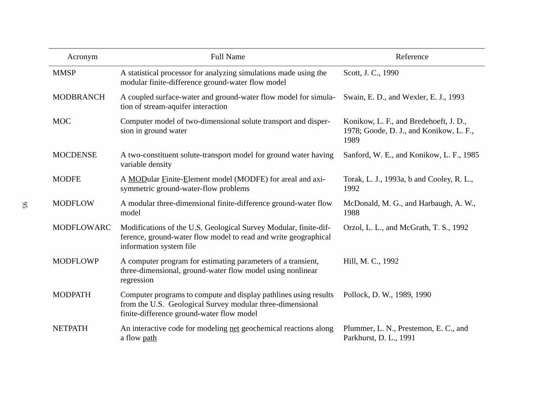
C., 1990
. D., and Wexler, E. J., 1993
, L. F., and Bredehoeft, J. D., oode, D. J., and Konikow, L. F.,
W. E., and Konikow, L. F., 1985
. J., 1993a, b and Cooley, R. L.,
ld, M. G., and Harbaugh, A. W.,
. L., and McGrath, T. S., 1992
C., 1992
D. W., 1989, 1990
r, L. N., Prestemon, E. C., and t, D. L., 1991
Reference
95
MMSP A statistical processor for analyzing simulations made using the modular finite-difference ground-water flow model
Scott, J.
MODBRANCH A coupled surface-water and ground-water flow model for simula-tion of stream-aquifer interaction
Swain, E
MOC Computer model of two-dimensional solute transport and disper-sion in ground water
Konikow1978; G1989
MOCDENSE A two-constituent solute-transport model for ground water having variable density
Sanford,
MODFE A MODular Finite-Element model (MODFE) for areal and axi-symmetric ground-water-flow problems
Torak, L1992
MODFLOW A modular three-dimensional finite-difference ground-water flow model
McDona1988
MODFLOWARC Modifications of the U.S. Geological Survey Modular, finite-dif-ference, ground-water flow model to read and write geographical information system file
Orzol, L
MODFLOWP A computer program for estimating parameters of a transient, three-dimensional, ground-water flow model using nonlinear regression
Hill, M.
MODPATH Computer programs to compute and display pathlines using results from the U.S. Geological Survey modular three-dimensional finite-difference ground-water flow model
Pollock,
NETPATH An interactive code for modeling net geochemical reactions along a flow path
PlummeParkhurs
Acronym Full Name

t, D. L., Thorstenson, D. C., and r, L. N., 1980 (Revised edition - 990)
, G. W., and Plummer, L. N.,
r, L. N., Parkhurst, D. L.,, G. W., and Dunkle, S. A., 1988
. E., 1984
. E., and Harbaugh, A. W., 1993b
M. W., Jr., and Jones, B. F., 1986
. M., Voss, C. I., and Rubin, 986
H. I., 1990
l, J. D., and Kharaka, Y. K., 1989
aka, Y. K., and Barnes, Ivan, 1973
, Y., Gunter, W. D., Aggarwal, K., Perkins, E. H., and DeBraal, 88
Reference
96
PHREEQE PHREEQE-A computer program for geochemical calculations ParkhursPlummeAugust 1
PHRQINPT An interactive computer program for constructing input data sets to the geochemical simulation program PHREEQE
Fleming1983
PHRQPITZ A computer program incorporating Pitzer’s equations for calcula-tion of geochemical reactions in brines
PlummeFleming
RADFLOW A Galerkin finite-element flow model to predict the transient response of a radially symmetric aquifer
Reilly, T
RADMOD Computer program for the simulation of cylindrical flow to a well using the U.S. Geological Survey Modular Finite-Difference Ground-Water Flow Model
Reilly, T
SALT NORM A quantitative chemical-mineralogical characterization of natural waters
Bodine,
SATRA-CHEM Numerical simulation of advective-dispersive multisolute trans-port with sorption, ion exchange and equilibrium chemistry
Lewis, FJacob, 1
SHARP A quasi-three-dimensional finite-difference simulation model for freshwater and saltwater flow in layered coastal aquifer systems
Essaid,
SOLINPUT A computer code to create and modify input for the geochemical program SOLMINEQ.88
DeBraa
SOLMINEQ Solution-mineral equilibrium computations Khar
SOLMINEQ.88 A computer program for geochemical modeling of water-rock interactions
KharakaPradeepJ. D., 19
Acronym Full Name

E., Bedinger, M. S., and Terry,76
I., 1984a
. R., 1987
, P. C., Pinder, G. F., and Larson, 76
, P. C., 1975; Trescott, P. C., and S. P., 1976; Torak, L. J., 1982
M. I., 1979
E. G., Healy, R. W., and Weeks, 87
. W., 1990
nd Clark, 1969
l, A. H., and Jones, B. F., 1973; l, A. H., and Jones, B. F., 1974
r, L. N., Jones, B. F., andl, A. H., 1976 (Revised edition 1984)
., Nordstrom, D. K., and Jenne, 80
Reference
97
SUPERMOCK Simulation procedure for modeling transient water-table and arte-sian stress and response
Reed, J. J. E., 19
SUTRA A finite-element simulation model for saturated-unsaturated, fluid-density-dependent ground-water flow with energy transport or chemically-reactive single-species solute transport
Voss, C.
SUTRAPLOT A graphical display program for SUTRA Finite-Element Simula-tion Model
Souza, W
Trescott-2D Finite-difference model for aquifer simulation in two dimensions TrescottS. P., 19
Trescott-3D Finite-difference model for simulation of three-dimensional ground-water flow
TrescottLarson,
TRIAG A finite-element model for flow in a two-aquifer system Mallory,
VS2D Computer program VS2D to solve the equations of fluid flow in variably saturated porous media
Lappala,E. P., 19
VS2DT Simulation of solute transport in variably saturated porous media Healy, R
WATCHEM Chemical properties of ground water Barnes a
WATEQ A computer program for calculating chemical equilibrium of natu-ral waters
TruesdelTruesdel
WATEQF A FORTRAN IV version of WATEQ, A computer program for calculating chemical equilibrium of natural waters
PlummeTruesdelJanuary
WATEQ2 Additional and revised thermochemical data and computer code for WATEQ2--A computerized chemical model for trace and major element speciation and mineral equilibria of natural waters
Ball, J. WE.A., 19
Acronym Full Name

., Jenne, E. A., and Cantrell,981
., and Nordstrom, D. K., 1991
h, A. W., 1990
Reference
98
WATEQ3 A geochemical model with uranium added Ball, J. WM. W., 1
WATEQ4F Revised thermodynamic data base and test cases for calculating speciation of major, trace, and redox elements in natural waters
Ball, J. W
ZONEBUDGET A computer program for calculating subregional water budgets using results from the U.S. Geological Survey modular three-dimensional finite-difference ground-water flow model
Harbaug
Acronym Full Name