supernova simulations and strategies for the dark...
TRANSCRIPT

Supernova Simulations and Strategies
For the Dark Energy Survey
J. P. Bernstein1, R. Kessler2,3, S. Kuhlmann1,
R. Biswas1, E. Kovacs1, G. Aldering4, I. Crane1,5, C. B. D’Andrea6,
D. A. Finley7, J. A. Frieman2,3,7, T. Hufford1, M. J. Jarvis8,9, A. G. Kim4,
J. Marriner7, P. Mukherjee10, R. C. Nichol6, P. Nugent4, D. Parkinson10,
R. R. R. Reis7,11, M. Sako12, H. Spinka1, M. Sullivan13
ABSTRACT
We present an analysis of supernova light curves simulated for the upcoming Dark EnergySurvey (DES) supernova search. The simulations employ a code suite that generates and fitsrealistic light curves in order to obtain distance modulus/redshift pairs that are passed to acosmology fitter. We investigated several different survey strategies including field selection,supernova selection biases, and photometric redshift measurements. Using the results of thisstudy, we chose a 30 square degree search area in the griz filter set. We forecast 1) that thissurvey will provide a homogeneous sample of up to 4000 Type Ia supernovae in the redshiftrange 0.05<z<1.2, and 2) that the increased red efficiency of the DES camera will significantlyimprove high-redshift color measurements. The redshift of each supernova with an identified hostgalaxy will be obtained from spectroscopic observations of the host. A supernova spectrum willbe obtained for a subset of the sample, which will be utilized for control studies. In addition,we have investigated the use of combined photometric redshifts taking into account data fromboth the host and supernova. We have investigated and estimated the likely contamination fromcore-collapse supernovae based on photometric identification, and have found that a Type Iasupernova sample purity of up to 98% is obtainable given specific assumptions. Furthermore, wepresent systematic uncertainties due to sample purity, photometric calibration, dust extinctionpriors, filter-centroid shifts, and inter-calibration. We conclude by estimating the uncertainty onthe cosmological parameters that will be measured from the DES supernova data.
Subject headings: supernovae – cosmology: simulations
1Argonne National Laboratory, 9700 South Cass Av-enue, Lemont, IL 60439, USA
2Kavli Institute for Cosmological Physics, The Univer-sity of Chicago, 5640 South Ellis Avenue Chicago, IL 60637,USA
3Department of Astronomy and Astrophysics, The Uni-versity of Chicago, 5640 South Ellis Avenue Chicago, IL60637, USA
4E. O. Lawrence Berkeley National Laboratory, 1 Cy-clotron Rd., Berkeley, CA 94720, USA
5Department of Physics, University of Illinois atUrbana-Champaign, 1110 West Green Street, Urbana, IL61801-3080 USA
6Institute of Cosmology and Gravitation, Universityof Portsmouth, Dennis Sciama Building, Burnaby Road,
Portsmouth PO1 3FX, UK7Center for Particle Astrophysics, Fermi National Accel-
erator Laboratory, P.O. Box 500, Batavia, IL 60510, USA8Centre for Astrophysics, Science & Technology Re-
search Institute, University of Hertfordshire, Hatfield,Herts, AL10 9AB, UK
9Physics Department, University of the Western Cape,Cape Town, 7535, South Africa
10Department of Physics and Astronomy, Pevensey 2Building University of Sussex, Falmer Brighton BN1 9QH,UK
11Now at: Instituto de Fısica, Universidade Federal doRio de Janeiro C. P. 68528, CEP 21941-972, Rio de Janeiro,RJ, Brazil
12Department of Physics and Astronomy, University of
1
FERMILAB-PUB-11-681-A
Operated by Fermi Research Alliance, LLC under Contract No. DE-AC02-07CH11359 with the United States Department of Energy

Contents
1 Introduction 2
2 Supernova light curve simulation 4
2.1 SNANA . . . . . . . . . . . . . . . . 5
2.2 Simulation inputs . . . . . . . . . . 5
3 Survey strategy options and example
simulations 7
3.1 Fields, filters, and selection cuts . . 8
3.2 Light curves and SN statistics . . . 10
4 Redshift Determination 15
4.1 Role of Each Method of RedshiftDetermination . . . . . . . . . . . 15
4.2 Accuracy of photometric redshifts . 16
4.3 Photometric redshifts for hostswithout spectra . . . . . . . . . . . 17
5 Supernova analysis with spectro-
scopic redshifts 17
5.1 MLCS2k2 light curve fitting with fullpriors . . . . . . . . . . . . . . . . 17
5.2 MLCS2k2 light curve fitting with flatpriors & SALT2 fitting . . . . . . . 19
6 Type Ia supernova sample purity 21
6.1 Core collapse input rate . . . . . . 21
6.2 Relative fractions of core collapsetypes . . . . . . . . . . . . . . . . . 22
6.3 Core collapse brightness . . . . . . 22
6.4 Core collapse templates . . . . . . 22
6.5 Sample purity results . . . . . . . . 23
7 Supernova colors, dust extinction,
and infrared data 26
7.1 Sensitivity to AV and RV . . . . . 26
7.2 VIDEO survey and additional in-frared overlap . . . . . . . . . . . . 27
7.2.1 The DES+VIDEO overlap . 27
7.2.2 The DES+VIDEO super-nova sample . . . . . . . . . 27
Pennsylvania, 203 South 33rd Street, Philadelphia, PA19104, USA
13Department of Physics, Denys Wilkinson Building, Ox-ford University, Keble Road, Oxford, OX1 3RH, UK
8 Dark energy constraints from differ-
ent survey Strategies 30
8.1 Figure of Merit . . . . . . . . . . . 30
8.2 Systematic uncertainties . . . . . . 34
9 Discussion and summary 36
A Fractions of SNIa Host Galaxies Sat-
isfying Apparent-Magnitude Limits 39
B SNe systematic uncertainties in the
FoM calculation 42
B.1 Nuisance Parameters . . . . . . . . 43
1. Introduction
In the late 1990’s, observations of distant TypeIa supernovae (SNIa) provided the convincing ev-idence for the acceleration of cosmic expansion(Riess et al. 1998; Perlmutter et al. 1999). Dedi-cated supernova (SN) surveys covering cosmolog-ically relevant redshifts, such as the ESSENCESupernova Survey (Miknaitis et al. 2007; Foleyet al. 2009), Supernova Legacy Survey (SNLS,Astier et al. 2006; Conley et al. 2011), Sloan Dig-ital Sky Survey-II Supernova Survey (SDSS, Frie-man et al. 2008b; Sako et al. 2011), Carnegie Su-pernova Project (Hamuy et al. 2006; Stritzingeret al. 2011), Stockholm VIMOS Supernova SurveyII (Melinder et al. 2011), and Hubble Space Tele-scope searches (e.g., Strolger et al. 2004; Dawsonet al. 2009; Amanullah et al. 2010), have substan-tially improved the quantity and quality of SNIadata in the last decade. A previously unknownenergy-density component known as dark energy isthe most common explanation for cosmic accelera-tion (for a review, see Frieman et al. 2008a; Wein-berg et al. 2012). The recent SN data, in combina-tion with measurements of the cosmic microwavebackground (CMB) anisotropy and baryon acous-tic oscillations (BAO), have confirmed and con-strained accelerated expansion in terms of the therelative dark energy density (ΩDE) and equationof state parameter (w ≡ pDE/ρDE , where pDE
and ρDE are the pressure and density of dark en-ergy, respectively). The next generation of cosmo-logical surveys is designed to improve the measure-ment of w, and constrain its variation with time,from observations of the most powerful probes ofdark energy as suggested by the Dark Energy Task
2

Force (Albrecht et al. 2006): SNe, BAO, weaklensing, and galaxy clusters.
Future SN surveys face common issues, includ-ing the number and position of fields, filters, expo-sure times, cadence, and spectroscopic and photo-metric redshifts. Each study must optimize tele-scope allocations to return the best cosmologicalconstraints. The simulation analysis presented inthe paper is for the Dark Energy Survey14 (DES),which expects to see first-light in 2012. The DESwill carry out a deep optical and near-infrared sur-vey of 5000 square degrees of the South Galac-tic Cap (see Fig. 1) using a new 3 deg2 ChargeCoupled Device (CCD) camera (the Dark EnergyCamera, or “DECam,” Flaugher et al. 2010) to bemounted on the Blanco 4-meter telescope at theCerro Tololo Inter-American Observatory (CTIO).The DES SN component will use approximately10% of the total survey time during photomet-ric conditions and make maximal use of the non-photometric time, for a total SN survey of ∼1300hours. The DECam focal plane detectors (Estradaet al. 2010) are thick CCDs from Lawrence Berke-ley National Laboratory (LBNL), which are char-acterized by much improved red sensitivity rel-ative to conventional CCDs (see Fig. 2, as wellas Holland 2002; Groom et al. 2006; Diehl et al.2008). This will allow for deeper measurementsin the redder bands, which is of particular impor-tance for high-redshift SNe. This effect is shown inFig. 3, which plots simulated scatter in the SALT2
(Guy et al. 2007) SN color parameter (see §5.2)for the SDSS, SNLS, and DES. Note, in particu-lar, the superior high-redshift color measurementsin the DES deep fields (see §3.1). Details of thesimulation method can be found in §2. The im-plementation for the DES, e.g., an exposure timeof approximately an hour in the SDSS-like z pass-band per field per observation, is discussed in §3.
An accurate redshift determination (to ∼0.5%)is necessary to place a SN on the Hubble diagram.This can be obtained by taking a spectrum of theSN itself or of its host galaxy. A spectrum of theSN has the added advantage of providing a defini-tive confirmation of the SN type, and allowing forstudies of systematic variations, but is more diffi-cult to obtain. Follow-up spectroscopy of the hostgalaxy can be done at a later date, taking advan-
14http://www.darkenergysurvey.org
Fig. 1.—: The DES footprint. The white squaresindicate the locations of our current choice of fiveSN fields (see §3.1). For the survey strategiesconsidered in this analysis with additional shal-low fields, those fields are placed next to these fivefields. The size of the squares as shown is muchlarger than the 3 deg2 field of view of DECam inorder to make them easier to see in this Figure.The scale shows the log of r-band (as defined in§3.1) Galactic extinction in magnitudes.
tage of multi-object spectrograph capabilities toobtain many spectra at once. Photometric red-shifts can also be obtained using deep co-addedphotometry of the host galaxy, but the redshiftaccuracy is degraded, reducing the usefulness ofthe SN for cosmological measurements. The exist-ing SNIa samples from previous surveys include asubset of SNe with measured spectra consisting of∼1000 SNIa spread out over many surveys (Sulli-van et al. 2011; Amanullah et al. 2010, and refer-ences therein), and the remainder includes manymore SNe with host spectra or host and/or SNphotometric redshifts. The usefulness of the cur-rent photometric samples depends on the fractionof host galaxies that will be followed-up, a num-ber which is uncertain. The DES will identify upto ∼4000 high-quality SNIa, and plans a follow-upprogram to acquire SN spectra near peak for up to20% of this sample and host galaxy spectra for themajority of the remainder. For SNe that do nothave a follow-up or host galaxy spectrum taken, adeep co-add of images (>70 hours per season) willbe used to determine the host photometric red-shift. This host redshift will be further utilized asa prior for a combined SN photometric redshift fit.
In order to aid in the design of the DES SNsearch, we simulate expected DES SN observa-tions. We use the parametric SNANA code suite
3

Wavelength (nanometers)
400 500 600 700 800 900 1000
Tra
nsm
issi
on o
r Q
E
0
0.1
0.2
0.3
0.4
0.5
0.6
0.7
0.8
0.9
1
Wavelength (nanometers)
400 500 600 700 800 900 1000
Tra
nsm
issi
on o
r Q
E
0
0.1
0.2
0.3
0.4
0.5
0.6
0.7
0.8
0.9
1 DES griz totalSNLS griz totalDES CCD QESNLS CCD QE
g r i z
Fig. 2.—: Comparison of the SNLS (Regnaultet al. 2009) and DECam total transmission (H.Lin, private communication, 2011) for an airmassof 1.3. Also shown is the CCD quantum efficiency(QE). The total transmission includes the effectsof QE, the atmosphere, and the optical systems ofthe relevant cameras. Note the increased DES sen-sitivity at redder wavelengths. The DECam trans-mission is based on measurements of the full-sizefilters, which was not available during the simu-lations performed for this analysis. The assumedtransmission in this paper is about 10% smallerthan the measured values.
(Kessler et al. 2009b) that generates SN lightcurves using realistic models and takes into ac-count, e.g., seeing conditions, Galactic extinction,and CCD noise. In this work, we use the optical(λ < 1 µm) MLCS2k2 (Jha et al. 2007) and SALT2
(Guy et al. 2007) models and the optical+infraredSNooPy model (Burns et al. 2011). We chose toemploy the MLCS2k2 model because the inclusionof the straightforward reddening parametrizationfrom Cardelli et al. (1989) makes it easier to assesssystematic errors simply by varying the parame-ters. In contrast, the parametrization in SALT2 ismore complex which complicates the systematicsstudies. We further employ a light curve fitter,based on MLCS2k2 and SALT2 models, to obtain aprediction of the measured distance modulus, µ,
Redshift
0 0.2 0.4 0.6 0.8 1 1.2
Col
or R
MS
0
0.02
0.04
0.06
0.08
0.1
0.12
0.14
0.16 DES deep
DES shallowSNLSSDSS
Fig. 3.—: Simulation of the scatter in the SALT2
color parameter for the SDSS, SNLS, and DES su-pernova samples highlighting the red advantage ofthe DES. The simulation method and DES imple-mentation are discussed in §2 and §3, respectively.
for each SN. Measured redshifts are expected tocome from a combination of spectra and photo-metric redshifts from the host galaxy and SN, andresults are compared for these different scenarios.
The outline of the paper is as follows. Wepresent our method of SN light curve simulationin §2. We discuss the DES options and present ex-ample simulations in §3. Redshift determinations,both spectroscopic and photometric, are discussedin §4. Analysis options are presented in §5. Astudy of Type Ia sample purity is presented in §6.SN colors and dust extinction are discussed in §7,and projected cosmology constraints are presentedin §8. Finally, we summarize and discuss our re-sults in §9.
2. Supernova light curve simulation
In this section, we present our SN light curvesimulations in greater technical detail. We discussgeneral properties of SNANA in §2.1 and introduceour application to the DES in §2.2.
4

2.1. SNANA
We employ the SNANA package (Kessler et al.2009b) to simulate and fit Type Ia and Type Ibc/IISN light curves. We emphasize that while we areusing SNANA to investigate the capabilities of theDES, it was originally developed for and utilizedfor the analysis of observational SDSS SN data(Kessler et al. 2009a), was used by the Large Syn-optic Survey Telescope (LSST) collaboration toforecast SN observations (Abell et al. 2009), andcan be applied to any survey in general. Using thesimulation requires a survey-specific library thatincludes the survey characteristics, e.g., filters, ob-serving cadence, seeing conditions, zeropoints, andCCD characteristics.
For a rest-frame SN light curve model, such asMLCS2k2, the basic simulation steps are as follows:
1. pick a sky position, redshift from observedSN rate distributions, and sequence of ob-server and rest-frame observation times;
2. pick SN luminosity (∆) and V -band host-extinction (AV, the amount of dust extinc-tion in magnitudes from Cardelli et al. 1989)parameters randomly drawn from their dis-tributions;
3. generate a rest-frame light curve from theSN light curve model: e.g., magnitudes inthe U, B, V, R, & I filters (Bessell 1990)versus time;
4. add host-galaxy extinction to each rest-frame magnitude using AV (from Step 2above) and the CCM dust model fromCardelli et al. (1989);
5. add K-corrections (Nugent et al. 2002) totransform UBVRI to observer-frame fil-ters15;
6. add Galactic (Milky Way) extinction usingdata from Schlegel et al. (1998);
7. use survey zeropoints to translate above-atmosphere magnitudes into observed flux inCCD counts;
15K-corrections are needed in both the simulator and fitter,and are applied using a technique very similar to that inJha et al. (2007).
8. compute noise from the sky level, pointspread function (PSF), CCD readout noise(negligible for the DES), and signal Poissonstatistics;
9. In addition to steps 4 and 5 above, apply anad-hoc Gaussian smearing model of intrinsicSN color variations to obtain Hubble resid-uals that match observations.
We make use of three light-curve models thatare integrated into SNANA to simulate and fit SNlight curves: MLCS2k2, SALT2, and SNooPy. Notethat SNANA uses MINUIT (James 1994) for min-imization. The MLCS2k2 model is improved rela-tive to the Jha et al. (2007) code (see §5.1 andAppendix B of Kessler et al. 2009a), e.g., it fits influx instead of magnitudes and includes simulatedefficiency in the prior. A key difference betweenMLCS2k2 and SALT2 is that the former fits for a dis-tance for each SN while the latter does not. TheSALT2 light curve model in SNANA is accompaniedby a separate program called SALT2mu (Marrineret al. 2011) that is used to determine a distancefor each SN so that the MLCS2k2 and SALT2 fit re-sults can be treated in the same way (see §5.2 foradditional information).
2.2. Simulation inputs
Construction of a survey-specific library as in-put to the SN simulation is crucial to obtainingrealistic simulated light curves. For each DES SNobserving field, this library includes informationabout the survey cadence, filters, CCD gain andnoise, PSF, sky background level, and zeropointsand their fluctuations. The zeropoint encodes ex-posure time, atmospheric transmission, and tele-scope efficiency and aperture. These quantitiesvary with each exposure and so, for the DES study,we created a program which uses, among otherthings, the CTIO weather histories, ESSENCE ze-ropoint and PSF data, time gaps due to Blancocommunity use, and Moon brightness to estimatethe parameters for the DES simulation library.Table 1 shows example entries in this library, andwe now discuss the details of their creation.
The SN component of the DES is limited toabout 10% of the total survey photometric time.In all cases, after a certain period of time (ex-pected to be ∼8 days), if a SN field has not been
5
MJD/Filter PSF (pixels) σsky (e−) Zpt (mag)
55881.191/g 2.26 80 33.055881.199/r 2.16 151 34.555881.215/i 2.05 257 34.755881.238/z 1.79 651 35.655884.312/g 2.58 143 32.755884.328/r 2.62 220 34.355884.344/i 2.35 390 34.455885.188/z 2.83 764 35.7
Table 1:: Example DES SN simulation inputs for a4-day excerpt from a single, 6-month season where“σsky” is the sky noise in photoelectrons and “Zpt”is the zeropoint in magnitudes. Additional inputsthat are needed, but not shown in this Table, arethe RA & DEC of the field, CCD gain and noise,pixel size, and the contribution to the zeropointdue to fluctuations.
observed it becomes the top observational priorityof the survey even under photometric conditions.There are two main options being considered forthe decision procedure to observe in shorter inter-vals than 8 days: 1) make maximal use of non-photometric time based on an infrared cloud cam-era (RASICAM, Lewis et al. 2010), or 2) decidebased on the measured seeing, giving the non-SNDES components the best seeing for weak lensingand other science, and switch to the SN fields ifthe PSF is & 1′′. The final DES decision tree willprobably be a combination of these two. In thisanalysis we have simulated option #1.
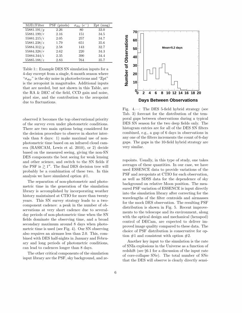
The separation of non-photometric and photo-metric time in the generation of the simulationlibrary is accomplished by incorporating weatherhistory maintained at CTIO for more than twentyyears. This SN survey strategy leads to a two-component cadence: a peak in the number of ob-servations at very short cadence due to several-day periods of non-photometric time when the SNfields dominate the observing time, and a broadsecondary maximum around 8 days when photo-metric time is used (see Fig. 4). Our SN observingalso requires an airmass less than 2.0. This, com-bined with DES half-nights in January and Febru-ary and long periods of photometric conditions,can lead to cadences longer than 8 days.
The other critical components of the simulationinput library are the PSF, sky background, and ze-
Days Between Observations
0 2 4 6 8 10 12 14 16 18 20
Num
ber
of O
bser
vatio
ns
0
10
20
30
40
50
60
70
Mean=5.2 days
Fig. 4.—: The DES 5-field hybrid strategy (seeTab. 3) forecast for the distribution of the tem-poral gaps between observations during a typicalDES SN season for the two deep fields only. Thehistogram entries are for all of the DES SN filterscombined, e.g., a gap of 6 days in observations inany one of the filters increments the count of 6-daygaps. The gaps in the 10-field hybrid strategy arevery similar.
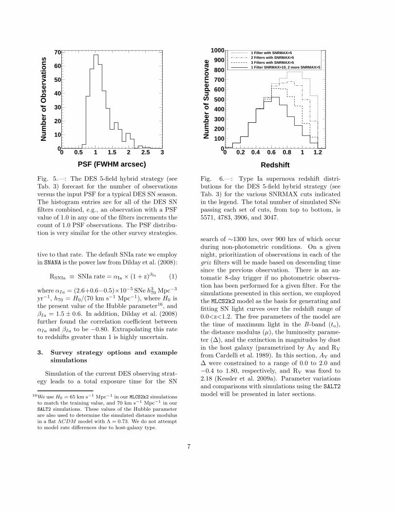
ropoints. Usually, in this type of study, one takesaverages of these quantities. In our case, we haveused ESSENCE data to provide variations of thePSF and zeropoints at CTIO for each observation,as well as SDSS data for the dependence of skybackground on relative Moon position. The mea-sured PSF variation of ESSENCE is input directlyinto the simulation library after correcting for thewavelengths of the filter centroids and airmassesfor the mock DES observation. The resulting PSFdistribution is shown in Fig. 5. Recent improve-ments to the telescope and its environment, alongwith the optical design and mechanical (hexapod)control of DECam, are expected to deliver im-proved image quality compared to these data. Thechoice of PSF distribution is conservative for op-tion #1 and consistent with option #2.
Another key input to the simulation is the rateof SNIa explosions in the Universe as a function ofredshift (see §6.1 for a discussion of the input rateof core-collapse SNe). The total number of SNethat the DES will observe is clearly directly sensi-
6
PSF (FWHM arcsec)
0 0.5 1 1.5 2 2.5 3
Num
ber
of O
bser
vatio
ns
0
10
20
30
40
50
60
70
Fig. 5.—: The DES 5-field hybrid strategy (seeTab. 3) forecast for the number of observationsversus the input PSF for a typical DES SN season.The histogram entries are for all of the DES SNfilters combined, e.g., an observation with a PSFvalue of 1.0 in any one of the filters increments thecount of 1.0 PSF observations. The PSF distribu-tion is very similar for the other survey strategies.
tive to that rate. The default SNIa rate we employin SNANA is the power law from Dilday et al. (2008):
RSNIa ≡ SNIa rate = αIa × (1 + z)βIa (1)
where αIa = (2.6+0.6−0.5)×10−5 SNe h370 Mpc−3
yr−1, h70 = H0/(70 km s−1 Mpc−1), where H0 isthe present value of the Hubble parameter16, andβIa = 1.5 ± 0.6. In addition, Dilday et al. (2008)further found the correlation coefficient betweenαIa and βIa to be −0.80. Extrapolating this rateto redshifts greater than 1 is highly uncertain.
3. Survey strategy options and example
simulations
Simulation of the current DES observing strat-egy leads to a total exposure time for the SN
16We use H0 = 65 km s−1 Mpc−1 in our MLCS2k2 simulationsto match the training value, and 70 km s−1 Mpc−1 in ourSALT2 simulations. These values of the Hubble parameterare also used to determine the simulated distance modulusin a flat ΛCDM model with Λ = 0.73. We do not attemptto model rate differences due to host-galaxy type.
Redshift
0 0.2 0.4 0.6 0.8 1 1.2
Num
ber
of S
uper
nova
e
0
100
200
300
400
500
600
700
800
900
1000 1 Filter with SNRMAX>52 Filters with SNRMAX>53 Filters with SNRMAX>51 Filter SNRMAX>10, 2 more SNRMAX>5
1 Filter with SNRMAX>52 Filters with SNRMAX>53 Filters with SNRMAX>51 Filter SNRMAX>10, 2 more SNRMAX>5
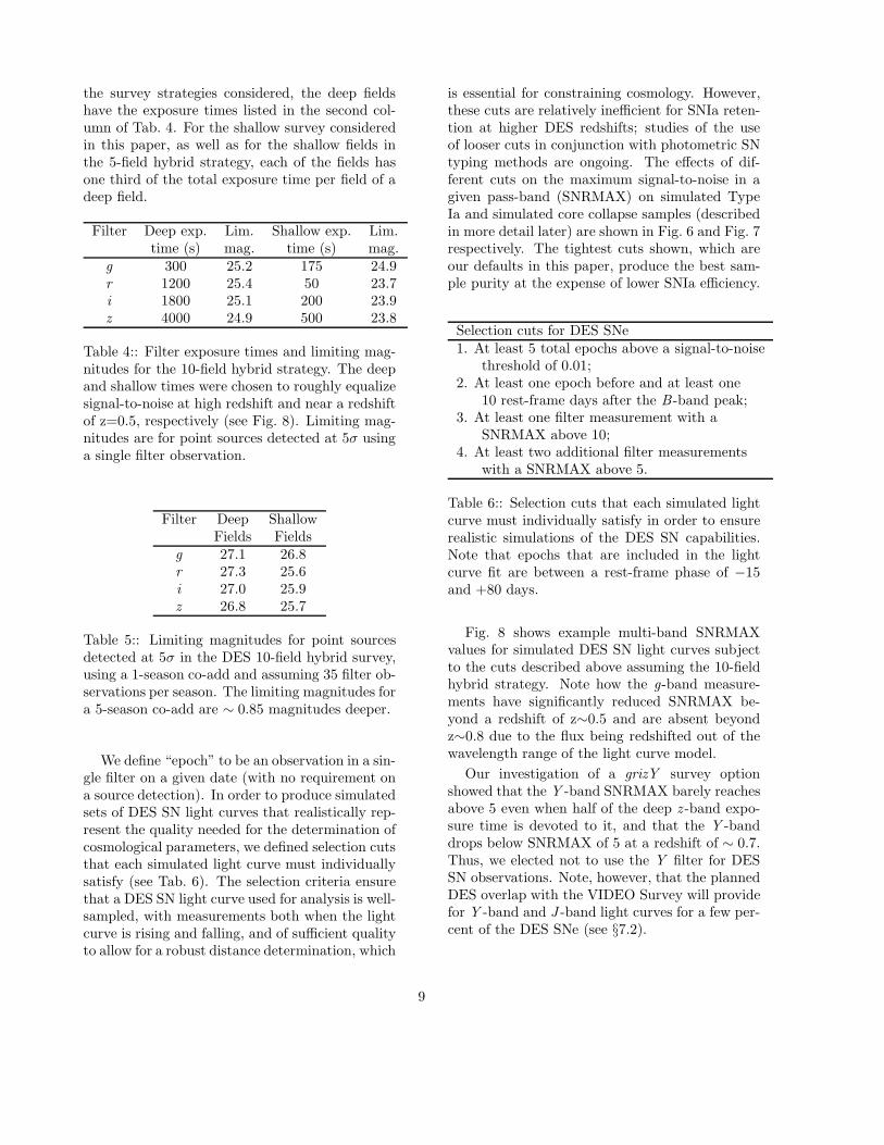
Fig. 6.—: Type Ia supernova redshift distri-butions for the DES 5-field hybrid strategy (seeTab. 3) for the various SNRMAX cuts indicatedin the legend. The total number of simulated SNepassing each set of cuts, from top to bottom, is5571, 4783, 3906, and 3047.
search of ∼1300 hrs, over 900 hrs of which occurduring non-photometric conditions. On a givennight, prioritization of observations in each of thegriz filters will be made based on descending timesince the previous observation. There is an au-tomatic 8-day trigger if no photometric observa-tion has been performed for a given filter. For thesimulations presented in this section, we employedthe MLCS2k2 model as the basis for generating andfitting SN light curves over the redshift range of0.0<z<1.2. The free parameters of the model arethe time of maximum light in the B -band (to),the distance modulus (µ), the luminosity parame-ter (∆), and the extinction in magnitudes by dustin the host galaxy (parametrized by AV and RV
from Cardelli et al. 1989). In this section, AV and∆ were constrained to a range of 0.0 to 2.0 and−0.4 to 1.80, respectively, and RV was fixed to2.18 (Kessler et al. 2009a). Parameter variationsand comparisons with simulations using the SALT2model will be presented in later sections.
7

Redshift
0 0.2 0.4 0.6 0.8 1 1.2
Num
ber
of S
uper
nova
e
0
100
200
300
400
500
600
700
800
900
1000 1 Filter with SNRMAX>52 Filters with SNRMAX>53 Filters with SNRMAX>51 Filter SNRMAX>10, 2 more SNRMAX>5
Fig. 7.—: Core-collapse supernova redshift distri-butions for the DES 5-field hybrid strategy (seeTab. 3) for the various SNRMAX cuts indicatedin the legend. The total number of simulated SNepassing each set of cuts, from top to bottom, is3458, 2462, 1785, and 1112.
3.1. Fields, filters, and selection cuts
The choice of the DES SN fields is driven byfour primary considerations:
• visibility from CTIO,
• visibility from Northern-hemisphere, 8-meter-class telescopes for SN follow-up spec-troscopy,
• past observation history as it pertains to theuse of pre-existing galaxy catalogs and cali-bration,
• overlap with the survey area for the Visible& Infrared Survey Telescope for Astronomy(VISTA, Emerson et al. 2004, see §7.2).
Based on these criteria, we have tentatively cho-sen the five fields in Tab. 2 and Fig. 1. In thispaper, we consider five SN survey strategies (seeTab. 3). For the 10-field hybrid strategy, the fieldsare the two deep fields and 3 shallow fields fromthe 5-field hybrid plus 5 additional shallow fieldsclustered around the Chandra Deep Field Southfield. In later sections we will compare in detail
the results of these surveys, including projectedconstraints on cosmology.
Field Pointing RA&Dec(3 deg2 area) (deg., J2000)
Chandra Deep Field S. 52.5, −27.5
XMM-LSS 34.5, −5.5
SDSS Stripe 82 55.0, 0.0
SNLS D1/Virmos VLT 36.75, −4.5
ELAIS S1 0.5, −43.0
Table 2:: Likely Dark Energy Survey supernovafields. Note that not all of these fields satisfyall of the field choice optimization criteria dis-cussed in the text; e.g., ELAIS S1 is not visi-ble from Northern-hemisphere, 8-meter-class tele-scopes, but matches the other criteria well.
Survey # deep # shallow Areastrategy fields fields (deg2)
ultra-deep 1 0 3deep 3 0 9
shallow 0 9 275-field hybrid 2 3 1510-field hybrid 2 8 30
Table 3:: Dark Energy Survey supernova strate-gies considered in this paper where each SN fieldhas an area equal to the DECam 3 deg2 field ofview. Note that the difference between deep andshallow fields is exposure time, not area.
We used SNANA to explore the choice of filtersand exposure times, and the resulting effects onsurvey cadence. We evaluated the effect of thegriz and grizY filter sets on DES SN observations.Figure 2 shows the chosen DES SN filters alongwith the DES CCD quantum efficiency. In thispaper, we have selected five SN search strategiesthat span the range from ultra-deep and narrowto wide and shallow, including hybrid mixtures ofthe two. Table 4 shows the filter exposure timesfor the deep fields for the deep and 10-field hy-brid strategies and the shallow fields for the 10-field hybrid strategy for the griz filter set (see thediscussion about Y -band at the end of this sec-tion). Table 5 shows the limiting magnitudes ineach filter for the 10-field hybrid survey. For all
8
the survey strategies considered, the deep fieldshave the exposure times listed in the second col-umn of Tab. 4. For the shallow survey consideredin this paper, as well as for the shallow fields inthe 5-field hybrid strategy, each of the fields hasone third of the total exposure time per field of adeep field.
Filter Deep exp. Lim. Shallow exp. Lim.time (s) mag. time (s) mag.
g 300 25.2 175 24.9r 1200 25.4 50 23.7i 1800 25.1 200 23.9z 4000 24.9 500 23.8
Table 4:: Filter exposure times and limiting mag-nitudes for the 10-field hybrid strategy. The deepand shallow times were chosen to roughly equalizesignal-to-noise at high redshift and near a redshiftof z=0.5, respectively (see Fig. 8). Limiting mag-nitudes are for point sources detected at 5σ usinga single filter observation.
Filter Deep ShallowFields Fields
g 27.1 26.8r 27.3 25.6i 27.0 25.9z 26.8 25.7
Table 5:: Limiting magnitudes for point sourcesdetected at 5σ in the DES 10-field hybrid survey,using a 1-season co-add and assuming 35 filter ob-servations per season. The limiting magnitudes fora 5-season co-add are ∼ 0.85 magnitudes deeper.
We define “epoch” to be an observation in a sin-gle filter on a given date (with no requirement ona source detection). In order to produce simulatedsets of DES SN light curves that realistically rep-resent the quality needed for the determination ofcosmological parameters, we defined selection cutsthat each simulated light curve must individuallysatisfy (see Tab. 6). The selection criteria ensurethat a DES SN light curve used for analysis is well-sampled, with measurements both when the lightcurve is rising and falling, and of sufficient qualityto allow for a robust distance determination, which
is essential for constraining cosmology. However,these cuts are relatively inefficient for SNIa reten-tion at higher DES redshifts; studies of the useof looser cuts in conjunction with photometric SNtyping methods are ongoing. The effects of dif-ferent cuts on the maximum signal-to-noise in agiven pass-band (SNRMAX) on simulated TypeIa and simulated core collapse samples (describedin more detail later) are shown in Fig. 6 and Fig. 7respectively. The tightest cuts shown, which areour defaults in this paper, produce the best sam-ple purity at the expense of lower SNIa efficiency.
Selection cuts for DES SNe1. At least 5 total epochs above a signal-to-noise
threshold of 0.01;2. At least one epoch before and at least one
10 rest-frame days after the B -band peak;3. At least one filter measurement with a
SNRMAX above 10;4. At least two additional filter measurements
with a SNRMAX above 5.
Table 6:: Selection cuts that each simulated lightcurve must individually satisfy in order to ensurerealistic simulations of the DES SN capabilities.Note that epochs that are included in the lightcurve fit are between a rest-frame phase of −15and +80 days.
Fig. 8 shows example multi-band SNRMAXvalues for simulated DES SN light curves subjectto the cuts described above assuming the 10-fieldhybrid strategy. Note how the g-band measure-ments have significantly reduced SNRMAX be-yond a redshift of z∼0.5 and are absent beyondz∼0.8 due to the flux being redshifted out of thewavelength range of the light curve model.
Our investigation of a grizY survey optionshowed that the Y -band SNRMAX barely reachesabove 5 even when half of the deep z -band expo-sure time is devoted to it, and that the Y -banddrops below SNRMAX of 5 at a redshift of ∼ 0.7.Thus, we elected not to use the Y filter for DESSN observations. Note, however, that the plannedDES overlap with the VIDEO Survey will providefor Y -band and J -band light curves for a few per-cent of the DES SNe (see §7.2).
9

3.2. Light curves and SN statistics
Fig. 9 shows example DES light curves at red-shifts of 0.25, 0.50, 0.74, and 1.07. Particularlynoteworthy is that the flux errors projected forDES SN observations are very small at lower red-shifts and remain reasonable even beyond a red-shift of z=1. The fact that the g-band is absentfor the z=0.74 and z=1.07 light curves highlightswhy high-redshift SNe only have 3 pass-bands forgriz surveys.
A key to planning a cosmological SN search isthe trade-off between survey area and depth. Forthe DES SN search, a motivation for deep observa-tions is the advantage of the DECam red sensitiv-ity, while a wide survey area is desirable because itreturns a greater number of SNIa at a given signal-to-noise. In other words, the observing strategyshould be both wide, to maximize SN statistics,and deep, to provide for a longer lever arm. Fig. 10shows the SNIa redshift distribution for the deep,shallow, and two hybrid survey strategies. We alsoconsidered an ultra-deep strategy (3 deg2). Wefound that the ultra-deep strategy delivers only amarginal improvement in SNIa statistics beyond aredshift of z=1 relative to the 10-field hybrid strat-egy, for example, while the latter results in a factorof 2.8 more SNIa overall. In particular, we foundthat the 10-field hybrid has 42% more SNIa in theredshift range of 0.6-1.0 relative to the ultra-deepstrategy. In addition, the ultra-deep survey pro-duces statistics inferior to the deep survey. Thus,the ultra-deep strategy is withdrawn from consid-eration, while the deep strategy is carried through-out this paper. Figure 10 also shows that the deepand shallow surveys exhibit a significant decreasein the number of SNe at low- and high-redshifts,respectively, relative to the two hybrid surveys.The hybrid surveys also retain a significant frac-tion of the low- and high-redshift SNe found in theshallow and deep surveys while avoiding a signif-icant fraction of the selection bias of the shallowsurvey (see §5.1). The redshift distributions forthe hybrid surveys including the deep and shallowcomponents are shown in Fig. 11. The 10-field hy-brid strategy is preferred on the grounds of max-imizing SN statistics in the intermediate redshiftregime.
In order to explore the sensitivity of the redshiftdistribution to the rate of SNIa, we performed
simulations including the αIa and βIa variationsaccording to the uncertainties given by Eqn. 1.Since Dilday et al. (2008) found the correlationcoefficient between αIa and βIa to be −0.80, weran simulations assuming the parameters are 100%anti-correlated. We found that the projected num-ber of DES SNIa would change by approximately7% given such a rate variation.
10

0 0.2 0.4 0.6 0.8 1 1.2
Ave
rage
SN
RM
AX
10
210
310 DES g-bandDES r-bandDES i-bandDES z-band
2 deep fields
Redshift
0 0.2 0.4 0.6 0.8 1 1.2
Ave
rage
SN
RM
AX
10
210
310
8 shallow fields
Fig. 8.—: Average maximum signal-to-noise forSNIa in a given pass-band (SNRMAX) for the 10-field hybrid strategy as a function of redshift in theDES g-, r -, i-, and z -bands. Note that at higherredshifts, the points are effected by the selectioncriteria. The upper and lower panels show theresult for the deep and shallow fields, respectively.
11

Phase (days)
0 50 100
Flu
x (a
rb. u
nits
)
0
100
200
z=0.25g band DES
Sim.
Phase (days)
0 50 100
0
100
200
r band
Phase (days)
0 50 100
0
100
200
i band
Phase (days)
0 50 100
0
100
200
z band
Phase (days)
0 50
Flu
x (a
rb. u
nits
)
0
20
40
z=0.50
Phase (days)
0 50
0
20
40
Phase (days)
0 50
0
20
40
Phase (days)
0 50
0
20
40
Phase (days)
0 50
Flu
x (a
rb. u
nits
)
0
20
40
z=0.74
Phase (days)
0 50
0
20
40
Phase (days)
0 50
0
20
40
Phase (days)
0 50
0
20
40
Phase (days)
0 50
Flu
x (a
rb. u
nits
)
0
20
40
z=1.07
Phase (days)
0 50
0
20
40
Phase (days)
0 50
0
20
40
Phase (days)
0 50
0
20
40
Fig. 9.—: From top to bottom: simulated DES light curves for the deep component of the 5-field hybridstrategy at redshifts of z=0.25, 0.50, 0.74, and 1.07, respectively. The points are MLCS2k2 simulated data,the center of the band is the MLCS2k2 fit, and the width of the band gives the fit error. Note the fluxaccuracy and progressive reduction in g-band flux until it drops out entirely due being redshifted out of thewavelength range of the light curve model.
12

Redshift
0 0.2 0.4 0.6 0.8 1 1.2
Num
ber
of S
uper
nova
e
0
100
200
300
400
500
600
700
800 shallow-9 fields
hybrid-10 fields
hybrid-5 fields
deep-3 fields
Fig. 10.—: Number of SNIa versus redshift for four of the DES strategies investigated. Total supernovastatistics are 4175, 3482, 2984, 2381 for the shallow 9-field, hybrid 10-field, hybrid 5-field, and deep 3-fieldsurveys respectively. The SN statistics shown include the application of all the selection cuts listed in Tab. 6.Note that subtle changes in the amount of exposure time allocated to each pass band can lead to large changesin the number of SNIa passing cuts. For example, a reasonable set of alternate exposure times consideredfor the 10-field hybrid results in ∼600 more SNIa passing cuts, mostly in the redshift range of 0.6-0.8. Suchadditional SNIa negate the apparent advantage of the 5-field hybrid survey in that redshift range as shownin this plot.
13

Redshift
0 0.2 0.4 0.6 0.8 1 1.2
Num
ber
of S
uper
nova
e
0
100
200
300
400
500Hybrid-5 fields2 deep fields3 shallow fields
Redshift
0 0.2 0.4 0.6 0.8 1 1.2
Num
ber
of S
uper
nova
e
0
100
200
300
400
500
600
700Hybrid-10 fields2 deep fields8 shallow fields
Fig. 11.—: Top (bottom): the SNIa redshift distribution for the 5-field (10-field) hybrid survey including thedeep and shallow components. Note that the 10-field cadence is slightly worse.
14

4. Redshift Determination
A precise estimate of SN redshifts is needed forplacement of SNe on the Hubble diagram and forperforming K-corrections on observed pass-bandsto the SN rest frame. There are four possiblemethods of obtaining SN redshifts: 1) spectro-scopic follow-up of individual SNe, 2) spectro-scopic redshifts of the associated host galaxies, 3)photometric redshifts (photo-z’s) of SNe, and 4)photo-z’s of the host galaxies. In addition, theDES collaboration is considering the use of opti-cal cross-correlation filters (Scolnic et al. 2009) forboth redshift determinations and SN typing. Thefinal analysis of the DES SNe will use the hostspectroscopic redshifts as the central method forredshift determination, with important roles beingplayed by the other methods. We next discuss theredshift determinations for the final analysis (withthe complete sample of host galaxy spectra andredshifts), as well as the interim analysis beforehost spectroscopic redshifts have been measured.
4.1. Role of Each Method of Redshift De-
termination
In previous SNIa Hubble diagram analyses,cosmological constraints have been obtained us-ing mostly spectroscopic confirmation of the SN,which not only afforded an extremely precise de-termination of the redshift, but also the additionaladvantage of accurate SN typing. For the DES, itis impractical to obtain spectra for every SN athigh-z. The DES will use photometric typing formost of the SNe observed (see §6). This techniqueworks very well, and will be further validated byobtaining a spectrum for a significant fraction oflow-redshift SNe. In addition, a sample of 10−20%of SNe at higher redshifts, with a spectrum takenwith 6-10m class telescopes, will be used to studySN evolution, photo-z’s, and sample purity. Notethat SNe with host galaxies too dim to obtain ahost spectrum are another sample that could trig-ger taking of a follow-up SN spectrum.
Obtaining spectroscopic redshifts of host galax-ies, assuming correct host identification, yieldsprecise SN redshifts. In addition, large numbers ofthe host galaxies can be measured simultaneouslywith a multi-object spectrograph (MOS). We willtarget every visible SN host, but we expect thatthe efficiency of obtaining a valid redshift will de-
Redshift SNLS Data Model0.1-0.2 100% 98%0.2-0.3 94.4% 97%0.3-0.4 97.4% 94%0.4-0.5 96.5% 92%0.5-0.6 94.1% 89%0.6-0.7 79.0% 85%0.7-0.8 88.6% 82%0.8-0.9 78.4% 78%0.9-1.0 76.9% 74%1.0-1.1 50.0% 70%1.1-1.2 N/A 67%
Table 7:: Measured (SNLS, Hardin et al., in prepa-ration) and estimated percentages of SNIa hostgalaxies with mi < 24 are tabulated. The modelvalues are taken from the middle column of Tab. 19from Appendix A. For both the data and model,the uncertainties grow from a few % at low redshiftto ±25% for z>1.0.
crease significantly for galaxies dimmer than ap-parent i-band magnitude mi = 24, as indicatedby the followup of SNLS galaxies (Hardin et al.,in preparation). For the purposes of our study,we have approximated the efficiency of obtaininga galaxy redshift as 100% for mi < 24 and 0% formi > 24. For forecasting SNe analyses, as wellas planning follow-up telescope resources, it is im-portant to estimate the fraction of SN hosts withmi < 24. Measurements of SNIa host magnitudesfrom SNLS (Hardin et al., in preparation) havelarge statistical uncertainties at the highest SNLSredshifts. Therefore, we have constructed a modeldescribed in Appendix A. This is a non-trivialtask, however, given uncertainties in the SNIa ratedependencies on galaxy mass, luminosity, and typeand of redshift evolution. Appendix A describes,in detail, our estimates of SNIa host galaxy bright-nesses in redshift bins, and the sources of signif-icant uncertainty at large redshift. A model es-timate is shown in Tab. 7, where we present thefractions of SNIa host galaxies satisfying the ap-parent magnitude limit mi < 24 for z-bin valuesfrom 0.1 to 1.2. Within the uncertainties, the dataand model agree. In this study, we choose to usethe model (since it lacks the statistical fluctuationsof the data) to remove from our cosmology analy-sis SNe without a host spectrum by applying thestated fractions (for the 10-field hybrid strategy,
15
05101520253035404550
True z0 0.2 0.4 0.6 0.8 1 1.2 1.4
Hos
t Pho
to z
0
0.2
0.4
0.6
0.8
1
1.2
1.4
05101520253035404550
True z0 0.2 0.4 0.6 0.8 1 1.2 1.4
SN
+Hos
t Pho
to z
0
0.2
0.4
0.6
0.8
1
1.2
1.4
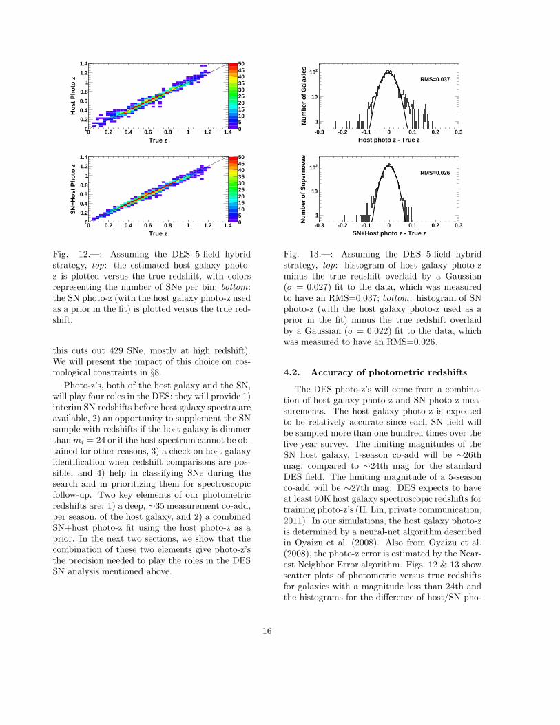
Fig. 12.—: Assuming the DES 5-field hybridstrategy, top: the estimated host galaxy photo-z is plotted versus the true redshift, with colorsrepresenting the number of SNe per bin; bottom:the SN photo-z (with the host galaxy photo-z usedas a prior in the fit) is plotted versus the true red-shift.
this cuts out 429 SNe, mostly at high redshift).We will present the impact of this choice on cos-mological constraints in §8.
Photo-z’s, both of the host galaxy and the SN,will play four roles in the DES: they will provide 1)interim SN redshifts before host galaxy spectra areavailable, 2) an opportunity to supplement the SNsample with redshifts if the host galaxy is dimmerthan mi = 24 or if the host spectrum cannot be ob-tained for other reasons, 3) a check on host galaxyidentification when redshift comparisons are pos-sible, and 4) help in classifying SNe during thesearch and in prioritizing them for spectroscopicfollow-up. Two key elements of our photometricredshifts are: 1) a deep, ∼35 measurement co-add,per season, of the host galaxy, and 2) a combinedSN+host photo-z fit using the host photo-z as aprior. In the next two sections, we show that thecombination of these two elements give photo-z’sthe precision needed to play the roles in the DESSN analysis mentioned above.
Host photo z - True z-0.3 -0.2 -0.1 0 0.1 0.2 0.3
Num
ber
of G
alax
ies
1
10
210RMS=0.037
SN+Host photo z - True z-0.3 -0.2 -0.1 0 0.1 0.2 0.3
Num
ber
of S
uper
nova
e
1
10
210RMS=0.026
Fig. 13.—: Assuming the DES 5-field hybridstrategy, top: histogram of host galaxy photo-zminus the true redshift overlaid by a Gaussian(σ = 0.027) fit to the data, which was measuredto have an RMS=0.037; bottom: histogram of SNphoto-z (with the host galaxy photo-z used as aprior in the fit) minus the true redshift overlaidby a Gaussian (σ = 0.022) fit to the data, whichwas measured to have an RMS=0.026.
4.2. Accuracy of photometric redshifts
The DES photo-z’s will come from a combina-tion of host galaxy photo-z and SN photo-z mea-surements. The host galaxy photo-z is expectedto be relatively accurate since each SN field willbe sampled more than one hundred times over thefive-year survey. The limiting magnitudes of theSN host galaxy, 1-season co-add will be ∼26thmag, compared to ∼24th mag for the standardDES field. The limiting magnitude of a 5-seasonco-add will be ∼27th mag. DES expects to haveat least 60K host galaxy spectroscopic redshifts fortraining photo-z’s (H. Lin, private communication,2011). In our simulations, the host galaxy photo-zis determined by a neural-net algorithm describedin Oyaizu et al. (2008). Also from Oyaizu et al.(2008), the photo-z error is estimated by the Near-est Neighbor Error algorithm. Figs. 12 & 13 showscatter plots of photometric versus true redshiftsfor galaxies with a magnitude less than 24th andthe histograms for the difference of host/SN pho-
16

Host photo z - True z-0.3 -0.2 -0.1 0 0.1 0.2 0.3
Num
ber
of G
alax
ies
05
1015202530354045
0.8<z<1.0 RMS=0.074
SN+Host photo z - True z-0.3 -0.2 -0.1 0 0.1 0.2 0.3
Num
ber
of S
uper
nova
e
0
10
20
30
40
50
60 With Host Prior0.8<z<1.0
RMS=0.053
Fig. 14.—: Using simulated photo-z’s trained ona sample with mi < 24, but applied to a dim-mer sample with 24 < mi < 26, the photo-zprecision is presented for 0.8 < z < 1.0 for theDES 5-field hybrid strategy. Top: Histogramof host galaxy photo-z minus the true redshift(RMS=0.074, σ = 0.047); note that there are 514total entries with 19 underflows and 9 overflows.Bottom: histogram of SNe photo-z (with the hostgalaxy photo-z used as a prior in the fit) minusthe true redshift (RMS=0.053, σ = 0.042). Simi-lar histograms for 1.0 < z < 1.2 demonstrate thefollowing widths: Host galaxy only (RMS=0.09,σ = 0.059), SN with host prior (RMS=0.079,σ = 0.045); note that there are 514 total entrieswith 4 underflows and 0 overflows
tometric redshifts and true redshifts, respectively.The host galaxy photo-z’s have a Gaussian sigmaof ∼0.027 and a non-Gaussian tail. The SN photo-z is fit with SNANA, using the host galaxy photo-zas a prior (Kessler et al. 2010a), is seen to have aGaussian sigma of ∼0.022 and much-reduced tails.When added to the spectroscopic redshifts pro-vided by SN follow-up, these redshifts are preciseenough to begin an interim analysis of DES SNebefore host spectra are available.
4.3. Photometric redshifts for hosts with-
out spectra
The second role for photo-z’s is to supplementredshifts from host spectra at high-z, assumingthe host spectra are only available for mi < 24.We have prepared a simulated sample (detailed inAppendix A) of galaxy photo-z’s that has beentrained on a sample of mi < 24 galaxies, but hasthen been applied to galaxies with 24 < mi <26. Fig. 14 shows histograms of the host photo-z residuals from this sample, and the combinedSNe+host photo-z. We will investigate the impactof using these photo-z’s on a cosmology analysis in§8.
At this time, we are assuming that SNe withhosts dimmer than mi = 26 will not be used in acosmology analysis, although with a 5-season co-add it is likely that many of those hosts will beobserved and may provide an interesting sampleto study.
5. Supernova analysis with spectroscopic
redshifts
In this section, we discuss SNIa analysis forthe case where every SN has a spectroscopic host-galaxy redshift, and correct SNIa identification isassumed (see §6), with an emphasis on the extrac-tion of distance estimates. In order to enhancethe robustness of our results, we employ both theMLCS2k2 and SALT2 models to simulate and fit SNlight curves. For MLCS2k2, we consider cases of fit-ting both with and without correct priors on hostgalaxy extinction.
5.1. MLCS2k2 light curve fitting with full
priors
The use of a prior on the MLCS2k2 extinction pa-rameter AV improves the determination of the dis-tance modulus when the measurement error on AV
becomes wider than the width of the AV distribu-tion. The improvement is noticeable in the simu-lated DES data at high redshifts where the SN col-ors are determined by measurements in only threebands: r, i, and z. However, the use of a prioris susceptible to the introduction of biases if im-plemented with incorrect information. While mea-surement errors, in principle, average to zero whenthe measurements of many SNe are combined, a
17
bias in the prior will not average to zero. Inaccu-racies in the prior, which is essentially the distri-bution of SNe in AV, can arise from purely exper-imental errors. However, unknown astrophysics,including the evolution of the host galaxy popu-lation or the SN colors with redshift, pose seriouschallenges to the use of a prior in a high precisionsurvey like the DES. While we do provide someestimate of potential systematic errors resultingfrom the use of a prior based on the SDSS anal-ysis, our estimates must currently be consideredpreliminary.
For the analysis presented here, the prior hasthe following definition:
Pprior = P (AV) × P (∆) × ǫcuts(z, AV, ∆), (2)
where P (AV) & P (∆) are the underlying physi-cal AV & ∆ (luminosity parameter) distributionsand ǫcuts is the fraction of SNe that pass the selec-tion cuts for a given redshift, AV, & ∆. For thiswork, following Kessler et al. (2009a), P (AV) isgiven by dN/dAV = exp(−AV/τAV
) with τAV=
0.334, and P (∆) is an asymmetric Gaussian withpeak position, ∆0, and positive and negative sidewidths, σ+ and σ−, respectively, given by ∆0 =−0.24, σ+ = +0.48, σ− = +0.23. In addition, weset dN/dAV=0 for AV<0.
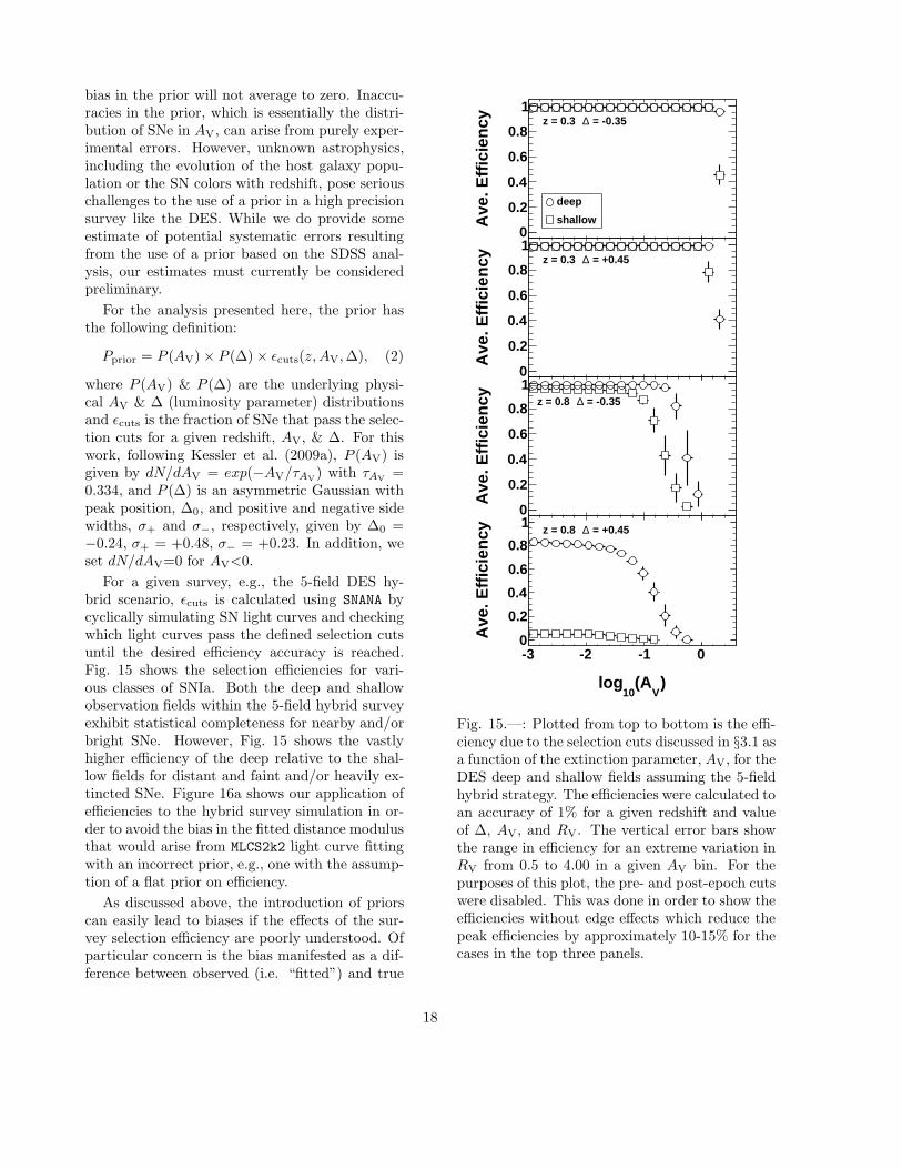
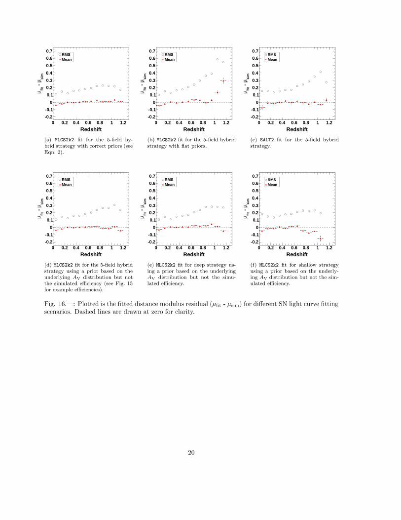
For a given survey, e.g., the 5-field DES hy-brid scenario, ǫcuts is calculated using SNANA bycyclically simulating SN light curves and checkingwhich light curves pass the defined selection cutsuntil the desired efficiency accuracy is reached.Fig. 15 shows the selection efficiencies for vari-ous classes of SNIa. Both the deep and shallowobservation fields within the 5-field hybrid surveyexhibit statistical completeness for nearby and/orbright SNe. However, Fig. 15 shows the vastlyhigher efficiency of the deep relative to the shal-low fields for distant and faint and/or heavily ex-tincted SNe. Figure 16a shows our application ofefficiencies to the hybrid survey simulation in or-der to avoid the bias in the fitted distance modulusthat would arise from MLCS2k2 light curve fittingwith an incorrect prior, e.g., one with the assump-tion of a flat prior on efficiency.
As discussed above, the introduction of priorscan easily lead to biases if the effects of the sur-vey selection efficiency are poorly understood. Ofparticular concern is the bias manifested as a dif-ference between observed (i.e. “fitted”) and true
-3 -2 -1 0
Ave
. Effi
cien
cy
0
0.2
0.4
0.6
0.8
1
deep
shallow
= -0.35∆z = 0.3
-3 -2 -1 0
Ave
. Effi
cien
cy
0
0.2
0.4
0.6
0.8
1 = +0.45∆z = 0.3
-3 -2 -1 0
Ave
. Effi
cien
cy
0
0.2
0.4
0.6
0.8
1 = -0.35∆z = 0.8
)V
(A10
log
-3 -2 -1 0
Ave
. Effi
cien
cy
0
0.2
0.4
0.6
0.8
1 = +0.45∆z = 0.8
Fig. 15.—: Plotted from top to bottom is the effi-ciency due to the selection cuts discussed in §3.1 asa function of the extinction parameter, AV, for theDES deep and shallow fields assuming the 5-fieldhybrid strategy. The efficiencies were calculated toan accuracy of 1% for a given redshift and valueof ∆, AV, and RV. The vertical error bars showthe range in efficiency for an extreme variation inRV from 0.5 to 4.00 in a given AV bin. For thepurposes of this plot, the pre- and post-epoch cutswere disabled. This was done in order to show theefficiencies without edge effects which reduce thepeak efficiencies by approximately 10-15% for thecases in the top three panels.
18

(i.e., “simulated”) distance modulus (“µfit” and“µsim” hereafter) that can arise. Figure 16f showssuch a departure of µfit – µsim from zero beyonda redshift of ∼0.7. The bias illustrates the size ofthe µ-correction that the DES SN data would needif the efficiency prior were incorrectly assumed tobe flat. Note, one does not expect the selectionbias to have a significant effect at low redshift be-cause there the SN sample is essentially complete.The fact that AV is driven toward zero, while thetrend in ∆ is negative, as redshift increases beyond∼0.5 (see Fig. 17), implies that only less extinctedand/or brighter SNe pass the selection cuts, andstrongly supports our identification of the bias inµ as a selection bias. In addition, this selectioneffect explains the small drop in RMS beyond aredshift of z=1.0 exhibited in Fig. 16a. Figure 16dalso shows, when compared to Fig. 16f, one of thekey motivations for the hybrid survey. A system-atic check is enabled by the ability to compare theless biased distance moduli from the deep part ofthe dataset at higher redshifts with the more bi-ased shallow part. If that crosscheck is validated,then confidence is increased in the highest regionof the deep component of the survey (i.e., redshiftsgreater than 1.0) where the deep component suf-fers a similar bias to that experienced by the shal-low component at intermediate redshifts. Fig. 16e,showing the case of the deep-only strategy, is in-cluded for completeness.
5.2. MLCS2k2 light curve fitting with flat
priors & SALT2 fitting
In this section, we discuss MLCS2k2 flat-priorand SALT2 model fitting. Such fits avoid the issueof selection efficiency bias discussed above. Thetrade-off is an increase in the RMS spread in thedistance modulus, as is clearly evident in the com-parison of Fig. 16a with Fig. 16b. In addition,Fig. 16b shows a high-redshift µ bias evident inMLCS2k2 fits with flat priors. This is due to thefact that such fits allow negative values of AV, forwhich the fitter compensates by pulling the dis-tance modulus to higher values.
The SALT2 light curve fitter in SNANA is ac-companied by a separate program called SALT2mu
(Marriner et al. 2011) that fits the SALT2 parame-ters α and β that are used to determine the stan-dard SNIa magnitudes. The parameters that cor-relate distance modulus with x1 (a stretch-like pa-
rameter) and c (the color) are α and β respectively.We have chosen to fit for the α and β parame-ters independent of the cosmology using SALT2mu,which allows us to apply the same cosmologicalfitting procedure to the outputs of the MLCS2k2
and SALT2 light curve fits.
The resulting distance modulus residuals areshown in Fig. 16c. The trend in the RMS spreadof the distance modulus is rather similar to thatobtained with MLCS2k2 with the use of a flat prior.While it would be possible to apply a prior on thecolor in the SALT2 fit, we have followed normalpractice in not doing so here. For the remainderof this paper, we will use MLCS2k2 fits with correctpriors (corresponding to Fig. 16a) in our analysis,with the exception that we use SNooPy in §7.2 andinclude SALT2 in the discussion of the DES SNcosmology fits in §8.
19
Redshift0 0.2 0.4 0.6 0.8 1 1.2
sim
µ -
fitµ
-0.2
-0.1
0
0.1
0.2
0.3
0.4
0.5
0.6
0.7RMSMean
(a) MLCS2k2 fit for the 5-field hy-brid strategy with correct priors (seeEqn. 2).
Redshift0 0.2 0.4 0.6 0.8 1 1.2
sim
µ -
fitµ
-0.2
-0.1
0
0.1
0.2
0.3
0.4
0.5
0.6
0.7RMSMean
(b) MLCS2k2 fit for the 5-field hybridstrategy with flat priors.
Redshift0 0.2 0.4 0.6 0.8 1 1.2
sim
µ -
fitµ
-0.2
-0.1
0
0.1
0.2
0.3
0.4
0.5
0.6
0.7RMSMean
(c) SALT2 fit for the 5-field hybridstrategy.
Redshift0 0.2 0.4 0.6 0.8 1 1.2
sim
µ -
fitµ
-0.2
-0.1
0
0.1
0.2
0.3
0.4
0.5
0.6
0.7RMSMean
(d) MLCS2k2 fit for the 5-field hybridstrategy using a prior based on theunderlying AV distribution but notthe simulated efficiency (see Fig. 15for example efficiencies).
Redshift0 0.2 0.4 0.6 0.8 1 1.2
sim
µ -
fitµ
-0.2
-0.1
0
0.1
0.2
0.3
0.4
0.5
0.6
0.7RMSMean
(e) MLCS2k2 fit for deep strategy us-ing a prior based on the underlyingAV distribution but not the simu-lated efficiency.
Redshift0 0.2 0.4 0.6 0.8 1 1.2
sim
µ -
fitµ
-0.2
-0.1
0
0.1
0.2
0.3
0.4
0.5
0.6
0.7RMSMean
(f) MLCS2k2 fit for shallow strategyusing a prior based on the underly-ing AV distribution but not the sim-ulated efficiency.
Fig. 16.—: Plotted is the fitted distance modulus residual (µfit - µsim) for different SN light curve fittingscenarios. Dashed lines are drawn at zero for clarity.
20

6. Type Ia supernova sample purity
Since the DES SNIa sample will not have fullspectroscopic SN follow-up, cases where core-collapse SNe (SNcc) are misidentified as SNIa willbe a concern for a cosmology analysis based onthe full sample. In order to address this issue,we have undertaken an analysis of the DES SNIasample purity using SNANA simulations. In thisstudy, we perform a mock-analysis using redshiftsdetermined from the visible host galaxies. Wehave limited measurements of SNcc types, rates,and brightness, but our knowledge of SNcc is lack-ing in several areas, as discussed in detail below.There are substantial uncertainties in the absoluterate of SNcc, mean absolute magnitudes and theirvariance, relative fractions of the different typesof SNcc, and variation in the light curve shapesthat are not adequately represented in the simula-tion. This section will address these uncertaintiesand provide estimates of their effect on SNIa sam-ple purity. In general, where there are choices tobe made, we make the choice that will increasethe amount of misidentification in order to seethe worst-case effect on a cosmology analysis, asdiscussed in §8.
6.1. Core collapse input rate
In order to simulate SNcc, we use the inputSN rate parametrization of Dilday et al. (2008),which found the SNIa rate from SDSS to be ofthe form α(1 + z)β with αIa = 2.6×10⁻⁵ withαIa = 2.6×10⁻⁵ SNe h3
70 Mpc−3 yr−1, and βIa =1.5. For SNcc, we take βcc = 3.6 to match the starformation rate. Various studies, the most recentbeing SNLS (Bazin et al. 2009), have shown thisassumption to be valid, albeit with low statisticsand limited redshift range. This leaves the deter-mination of αcc. Taking the ratio of SNcc/Ia to bethe SNLS value of 4.5 for redshifts of < 0.4 (Bazinet al. 2009), we calculate the value αcc must havein order to obtain the ratio of 4.5: αcc = 6.8×10⁻⁵
SNe h370 Mpc−3 yr−1. Note that with this value
of αcc, the SNcc/Ia ratio increases to ∼ 10 outto a redshift of 1.2. A caveat in this estimate isthat one of the largest uncertainties is the actualpopulation near the detection threshold. Directmeasurements of the SNcc rate beyond a redshiftof z=0.4 would be very helpful in the determina-tion of SNIa sample purity.
VFitted A0 0.5 1 1.50
200
400
600
∆Fitted -1 -0.5 0 0.5 10
200
400
600
Redshift0 0.2 0.4 0.6 0.8 1 1.2
VA
0
0.5
SimulatedFitted
Redshift0 0.2 0.4 0.6 0.8 1 1.2
∆
-0.5
0
SimulatedFitted
Fig. 17.—: Plotted from top to bottom is thefitted AV histogram, the fitted ∆ histogram, theredshift dependence of simulated & fitted AV, andredshift dependence of simulated & fitted ∆, bothaveraged within a redshift bin, assuming the 5-field hybrid strategy. Note that the lowest redshiftbin has low SN statistics (see Fig. 10).
21

6.2. Relative fractions of core collapse
types
In this section, we discuss the relative fractionof the SNcc subtypes. The most important frac-tion is that of Type Ib/c, since they most com-monly pass the combination of cuts on SNRMAXand MLCS2k2 fit-probability that the SN is a SNIa(fp=Pχ2 , the probability from fit χ2 and the num-ber of the degrees of freedom). The literature con-tains several estimates of the ratio of Type Ib/cto Type Ib/c plus II SNe (see Tab. 8 for exam-ples). The most complete references, in terms offractions being given for each type of SNcc, areLi et al. (2011a) and Smartt et al. (2009), andthe Type Ib/c fractions are in good agreement.We have used the Smartt et al. (2009) values (seeTab. 9) as the default set of fractions in this anal-ysis, as they give a more conservative amount ofSNcc misidentification relative to Li et al. (2011a).
Reference Ib/c fractionLi et al. (2011a) 24.6 ± 4.6%Li et al. (2007) 26.5 ± 5.4%
van den Bergh et al. (2005) 24.7 ± 2.6%Smartt et al. (2009) 29.3 ± 4.7%Prieto et al. (2008) 24.7 ± 4.9%
Leaman et al. (2011) 33.3 ± 4.3%
Table 8:: References for the relative fraction ofType Ib/c SNe (number of Type Ib/c divided bythe total number of SNcc of all types).
SN Type Relative SNcc FractionsIIP 0.587 ± 0.05Ib/c 0.293 ± 0.05
IIL + IIb 0.082 ± 0.03IIn 0.038 ± 0.02
Table 9:: The relative fraction of collapse SNe sub-types (number of a given subtype divided by totalnumber of SNcc of all types) used in this analysis,as taken from Smartt et al. (2009).
6.3. Core collapse brightness
The absolute brightness of SNcc is a critical pa-rameter in the number of SNcc misidentified asSNIa, since most are too dim to pass typical SNR-MAX cuts (e.g., those shown in Tab. 6). Two ref-
erences for absolute SNcc brightnesses, Richard-son et al. (2002) and Li et al. (2011a), are com-pared in Tab. 10 and Tab. 11. The numbers inTab. 10 have been corrected for the significantMalmquist bias evident in that data. The correc-tion assumed a threshold of 16 magnitudes in ap-parent brightness, and took into account the largervolume sampled by intrinsically brighter SNe thanfor fainter SNe. The volume-limited analysis in Liet al. (2011a) is already corrected for Malmquistbias, but Conley et al. (2011) used Richardsonet al. (2002) in their analysis, noting that Liet al. (2011a) perhaps missed a bright Type Ib/ccomponent by avoiding low-luminosity galaxies.To take the conservative approach, we used thesingle-Gaussian-approximation brightnesses fromRichardson et al. (2002) as our default.
Richardson et al. (2002)SN Type MB σMB
IIP −14.40± 0.42 0.81Ib/c −16.72± 0.23 0.62IIL −17.19± 0.15 0.47IIn −17.78± 0.41 0.74
Table 10:: The absolute B-band magnitudes andwidths for the single Gaussian fits from Richard-son et al. (2002), corrected for Malmquist bias.
Li et al. (2011a)SN Type MR σMR
IIP −15.66± 0.16 1.23Ib/c −16.09± 0.23 1.24IIL −17.44± 0.22 0.64IIn −16.86± 0.59 1.61
Table 11:: The absolute R-band magnitudes andwidths from Li et al. (2011a).
6.4. Core collapse templates
SNcc are observed to be a much more het-erogeneous class than SNIa and, in contrast toSNIa, there is no parametrization available thatdescribes the diversity of SNcc light curves. There-fore, we take a template approach to modelingSNcc. Three sets of templates are compared,with each being a spectral sequences as a func-tion of time. The first set are 40 templates from
22

the Supernova Photometric Classification Chal-lenge (Kessler et al. 2010b), the second set are thecomposite spectral templates constructed by Nu-gent17, and the third set are Type Ib/c and IIPtemplates from Sako et al. (2011), augmented bythe Nugent templates for Types IIL and IIn. Alltemplates were converted to SDSS filter magni-tudes, and SNANA performs the K-corrections intothe DES filters. Note that there is no templatefor Type IIb, which in Li et al. (2011a) is morenumerous than Types IIL or IIn. The Type IILtemplate is expected to be the closest to Type IIbSNe, and, therefore, we used it for the Type IIbsub-sample.
In the SNANA simulation, the templates are cor-rected to the absolute brightnesses discussed in theprevious section. In addition, the Nugent tem-plates are composite spectra and do not includeabsolute brightness fluctuations, therefore theyare also smeared by the Gaussian-fitted widthstabulated in the previous section in order to betterreflect the observations. The Kessler et al. (2010b)and Sako et al. (2011) templates already have suf-ficient variation in brightnesses and require no ad-ditional smearing. The templates from the Su-pernova Photometric Classification Challenge arethe most complete set and are used as the de-fault in the rest of this paper. In particular, notethat these templates contain a “1+ztemp” bug inthat each SNcc template is too dim by a factorof 1+ztemp (see Tab. 4 and §2.6 of Kessler et al.2010b), where ztemp is the redshift of the template.In the next section, we include a discussion of theeffect of this bug on our simulations.
6.5. Sample purity results
Using the inputs discussed above, and spectro-scopic host redshifts, we simulated the DES SNsample including SN Types Ia, Ib/c, IIL, IIn, andIIP subject to the selection criteria listed in Tab. 6.The SNe in this combined sample are fit to theSNIa MLCS2k2 model, giving a fit probability fp
variable cut that can be customized for each anal-ysis, and for the amount of SNcc observed in a sub-sample with spectroscopic follow-up. Figure 18shows the distribution of fp for the SNIa and SNccsamples, after all other selection cuts have been
17http://supernova.lbl.gov/%7Enugent/nugent templates.html;see also Nugent et al. (2002).
applied. The number of SNe of each type with nofp cut, and with fp > 0.1, is shown in Tab. 12. Forthose results, the effect of the 1+ztemp SNcc tem-plate bug discussed at the end of the previous is anincrease in the SNIa purity by ∼2%, which has noimpact on our conclusions. Figures 19 and 20 showredshift distributions of these samples subject toa fit probability cut fp > 0.1. Table 13 showscomparisons in the total SNcc number with vari-ations in the simulation inputs discussed above,with a range of ×3 in total sample SNcc. Notethat the sample purity is better than that ob-tained with the same analysis performed in Kessleret al. (2010b); this is due to the correction forMalmquist bias applied to the core collapse simu-lation sample, which reduces their expected abso-lute brightness and therefore the number passingSNRMAX cuts.
Sample fp >0.0 fp >0.1 Tot. simulatedIb/c 571 57 53514IIP 110 2 107210IIn 225 2 6940IIL 62 2 14976
Tot. SNcc 968 63 182640Ia 3482 3350 18695
Ia+SNcc 4450 3413 201335Ia Purity 78% 98.1% n/a
Table 12:: Number of simulated SNe passing cutsand sample purity using the DES 10-field hybridstrategy for SNIa fit probability, fp cuts of 0.0 and0.1. Note that employing fp > 0.2 reduces thenumber of SNIa and SNcc passing cuts by 5% and46%, respectively. However, given that the impactof SNcc on the DES cosmological constraints is al-ready negligible assuming fp > 0.1 (see §8), opt-ing for fp > 0.2 is unwarranted due to the loss ofSNIa. Note that these results were obtained withSNANA v8 37, which includes a known bug due toeach SNcc template being too dim by a factor of1+ztemp (see §2.6 of Kessler et al. 2010b), whereztemp is the redshift of the template. We haveverified that employing fixed versions, e.g., v9 89,results in a small (∼2%) purity variation that doesnot have an effect on our conclusions.
23

Simulation Input Total SNccDefaults 63
Nugent templates 27Sako et al. templates 44
Li et al. abs. magnitudes 8
Table 13:: Total SNcc counts with variations inthe simulation inputs assuming the 10-field hy-brid strategy, with fp >0.1. The line labeled “De-faults” is the same as the Total SNcc in Tab. 12.
SNIa Fit Probability
0 0.2 0.4 0.6 0.8 1
Num
ber
of S
uper
nova
e
0
200
400
600
800
1000
SNIa
SNcc
Fig. 18.—: Plotted are the SNIa fit probabilitiesfor the SNIa and SNcc samples, after all other se-lection cuts are applied.
24

Redshift0 0.2 0.4 0.6 0.8 1 1.2
Num
ber
of S
uper
nova
e
0
5
10
15
20
25
Ib/c
IIP+IIn+IIL
Fig. 19.—: Plotted are the histograms showing the projected DES redshift distributions for the TypeIb/c SNe and the summed distribution of other core collapse SNe, assuming the 10-field hybrid survey, theselections criteria in Tab. 6, and fp >0.1.
Redshift0 0.2 0.4 0.6 0.8 1 1.2
Num
ber
of S
uper
nova
e
0
200
400
600
800
1000
1200 Ia+Core Collapse
Core Collapse
Redshift0 0.2 0.4 0.6 0.8 1 1.2
Cor
e C
olla
pse
/ Tot
al
0
0.01
0.02
0.03
0.04
0.05
0.06
0.07
Fig. 20.—: Plotted are the redshift distributions for the projected DES SNIa and non-Ia SN samplesassuming the 10-field hybrid strategy, the selections criteria in Tab. 6, and fp >0.1.
25

7. Supernova colors, dust extinction, and
infrared data
The study of SN colors is a rich subject thatis of crucial importance to SN cosmology. The is-sue of confusion between intrinsic color variationsand dust extinction, which complicates the mea-surement of the former, is beyond the scope ofthis paper. Instead, we demonstrate the DES sen-sitivity to variations of the traditional, redshift-independent dust parameters AV and RV (Cardelliet al. 1989). Color measurements in the DES willbe improved by the enhanced red sensitivities ofthe CCDs, as discussed in §1.
Phase (days)
-5 0 5 10 15 20 25 30
(m
ags)
ref
⟩g-
z⟨
-
⟩g-
z⟨
-0.2
-0.15
-0.1
-0.05
0
0.05
0.1
0.15
0.2
Fig. 21.—: Average DES g − z color differenceversus phase assuming the 5-field hybrid strategyfor a simulation with RV = 2.69 and τAV
= 0.25,as compared to the reference simulation with RV
= 2.18 and τAV= 0.334. Error bars are the error
on the mean color difference. The solid, horizontalline above zero shows the fitted average g−z colordifference for phase < +11 days. Note that sincethe quantity plotted a difference between colors,the errors, which are the quadrature sum of theerrors on the mean of each color, are correspond-ingly large.
7.1. Sensitivity to AV and RV
We perform an analysis of the color variationsin the SN colors g − i, g − z, r − i, and r − z
for a grid of values of RV and τAV, where τAV
is the parameter that controls the width of thesimulated AV distribution, as described in §5.1.As τAV
increases, the AV distribution extends tolarger extinctions and, thus, produces SNe withredder colors. Our reference color sample is a sim-ulation with the values of RV = 2.18 and τAV
=0.334, which are the best fit values from Kessleret al. (2009a). The results presented here are forthe redshift range 0.4 <z< 0.7. This range has thehighest SN statistics for the DES. For the redshiftrange z< 0.4, the SN statistics are much less, butSNRMAX is substantially better, so that the pre-cision of the color measurements are comparableto those presented here.
VR
1.5 2 2.5 3
(m
ags)
ref
⟩g-
z⟨
-
⟩g-
z⟨
-0.2
-0.15
-0.1
-0.05
0
0.05
0.1
0.4 < z < 0.7
= 0.16τ = 0.33τ
= 0.52τ = 0.28τ = 0.39τ
Fig. 22.—: Average DES g− z color difference as-suming the 5-field hybrid strategy for phase < +11days compared to the reference simulation withRV = 2.18 and τAV
= 0.334 as a function of RV
and for a range of τAV. Error bars are the error on
the mean color difference. Note the isolated pointsfor τAV
= 0.28 and 0.39. We use these points toset the values of the 1σ errors in RV and τAV
tobe 0.38 and 0.06, respectively.
We constructed a suite of simulations with agrid of RV and τAV
values in order to assess the ef-fects of changes in RV and τAV
on SNIa colors. Anexample of the effects on the g − z color is shownin Fig. 21. The differences in color between sim-ulations with RV = 2.69 and τAV
= 0.25 and ourreference sample parameters is shown as a function
26

of phase. A signal-to-noise cut of 0.5 is applied atevery phase. Fig. 21 has two noteworthy features:the fitted average color level for phase < +11 daysand the significant drop in color for later phases.The average color level of a given SN color forphase < +11 days has, in general, a complicateddependence on RV, τAV
, and the redshift range ofthe data sample. In special cases, for simulationswith fixed RV, AV, and certain values of fixed red-shift, this dependence can be predicted from theCCM dust model (Cardelli et al. 1989) and theparametrization from Jha et al. (2007). We haveverified that our simulations agree well with thepredictions in these cases.
The sensitivity to parameters RV and τAVof
the small-phase average g − z difference is shownin Fig. 22. The error bars show the statistical un-certainty for each parameter choice. Overall, thetrend is to increase the value of the g − z differ-ence by approximately 0.3 magnitudes as RV in-creases from 1.1 to 3.1, which is a plausible rangefor RV, and τAV
increases from 0.16 to 0.52. Fromthis figure, simulated values of RV within ∼0.38of the reference value, and of τAV
within ∼0.06 ofthe reference value, can be distinguished at the 1σlevel. Similar plots for other SN colors and otherredshift ranges show slightly different dependen-cies on the parameters, and hence can be used tolower further the above uncertainties in RV andτAV
. Fig. 22 also shows several degenerate com-binations of RV and τAV
that lead to the samelevel of g − z difference. This occurs because SNcolors are largely dependent only on the ratio ofAV to RV, and so a given color difference can onlydetermine the ratio of AV to RV to some uncer-tainty. This degeneracy is reduced by consideringthe behaviors of other color differences and theirredshift dependence. In addition, the second fea-ture of Fig. 21, namely the drop-off in the g − zdifference at late phases18, can also be used to re-solve this degeneracy. In this analysis, we assumethat the degeneracy can be broken by an SDSS-like analysis (Kessler et al. 2009a), which took allsuch effects into consideration. Therefore, in ouranalysis in §8, we take the uncertainty in RV andτAV
to be 0.38 and 0.06, respectively.
18This drop-off is due to an effect of the SNRMAX cut: forredshifts greater than z ≈ 0.4, where the DES is no longerfully efficient, the SNRMAX cut is more likely to removethe fainter, redder SNe at late phases.
7.2. VIDEO survey and additional in-
frared overlap
7.2.1. The DES+VIDEO overlap
The infrared VISTA Deep Extragalactic Obser-vations (VIDEO) Survey (see, e.g., Jarvis 2009),using the Visible and Infrared Survey Telescope forAstronomy at the Paranal Observatory in north-ern Chile, began science observations in late 2009.This 5-year survey has an area of 12 deg2 covering4.5 deg2 in XMM-LSS, 4.5 deg2 in Chandra DeepField South, and 3 deg2 in ELAIS S1, with deepobservations in the Z, Y, J, H, K s filter set. Thesurvey is designed to trace galaxy evolution outto a redshift of 4, and also provides for a large-volume SN search projected to find 250 SNcc and100 SNIa with a median redshift of 0.2.
The VIDEO Survey SN fields overlap those forthe DES (see Tab. 2). The extension of opticalSNIa light curves to include infrared data pointsenables an enhanced determination of SN colorsand dust extinction due to the larger lever armprovided by the increased wavelength range. Asemphasized by Freedman et al. (2009), which pre-sented the first i-band Hubble diagram obtainedby the Carnegie SN Project, infrared SN observa-tions offer advantages in reducing several system-atic effects, the most notable of which is reddeningdue to dust. In particular, near-infrared observa-tions can be used to obtain a SN data set that isinsensitive to variations in SN color, and thereforefacilitate the best rate assessments for different SNtypes and their dependence on host galaxy proper-ties. In order to simulate expected results from acombined DES+VIDEO dataset, we incorporatedthe optical+infrared SNooPy SN light-curve model(Burns et al. 2011) into SNANA. Such a dataset,even with modest SN statistics, enables the pur-suit of reduced-extinction systematics studies.
7.2.2. The DES+VIDEO supernova sample
Based on VIDEO Survey SN data from the firstseason, we constructed a SNANA simulation library(see §2.2) with the following characteristics: typ-ical Y- and J-band PSF is of order 1 arcsec, skynoise on the order of 200-400 photoelectrons, andzeropoints ranging from 31.5 to 32.0 magnitudes.Two seasons of VIDEO/DES overlap are expected,and the simulation library assumes that the ob-serving conditions will be similar during both sea-
27

sons. In addition, there are 10 observations inY -band and 13 in J-band, each with 32 minutesof exposure time. Based on this simulation li-brary, we estimate that the DES+VIDEO com-bined SNIa sample from years 2013 and 2014 couldconsist of approximately 108 SNe with z<0.5 inthe common Chandra Deep Field South, XMM-LSS, and ELAIS S1 fields (see Tab. 2). Figures 23and 24 show VIDEO SNRMAX for the 108 over-lapping SNe, and an example simulated combinedlight curve, respectively. As shown in Fig. 23,some of the SNe have SNRMAX that are rela-tively low (e.g., < 5), and may not be useful forall SNe analyses. As a follow-on to this analy-sis, a study is planned to utilize SNANA simulatedDES+VIDEO SNIa light curves to evaluate thebenefit to SN color determinations to be gainedby adding VIDEO infrared SNIa data to the DESSN analysis.
Redshift
0 0.2 0.4
VID
EO
SN
RM
AX
10
210VIDEO Y-band
VIDEO J-band
Fig. 23.—: SNRMAX as a function of redshift forthe VIDEO Y - and J -bands.
28

0 50 100
Flu
x (a
rb.)
050
100150200250
z=0.25DES g band DES
Sim.
Phase (days)0 50 100
Flu
x (a
rb.)
050
100150200250 DES z band 0 50 100
050
100150200250 DES r band
Phase (days)0 50 100
050
100150200250 VIDEO Y band 0 50 100
050
100150200250 DES i band
Phase (days)0 50 100
050
100150200250 VIDEO J band
Fig. 24.—: Example simulated Type Ia SN light curve forecast displaying combined DES and VIDEOSurvey data assuming the DES 5-field hybrid strategy. The points are a MLCS2k2 fit and the band is thefit error. The wavelength ranges in nanometers of the pass-bands indicated are: 400–550 (g-band), 560–710(r -band), 700–850 (i-band), 850–1000 (z -band), 970–1020 (Y -band), 1040–1440 (J -band). Note that initialinvestigations show that the H and K s SNRMAX is insufficient for SN science, and so only a grizYJ lightcurve is shown.
29

8. Dark energy constraints from different
survey Strategies
In this section, we present a forecast of the con-straints on cosmological parameters from the DESSN search using our simulations of the differentsurvey strategies summarized in Tab. 3 (with theexception of the ultra-deep strategy, which is notconsidered here). In order to be included in theanalysis in this section, each SN is required to passthe selection criteria listed in Tab. 6. In order toensure an accurate spectroscopic host galaxy red-shift determination, SNe with faint hosts (mi <24) are discarded. A multi-color light curve fit foreach SN in the sample is made using the MLCS2k2
model with the prior listed in Eqn. 2, as describedin §5. In this section, we also include results us-ing the SALT2 model for comparison. A SNIa fitprobability cut of 0.1 (fp > 0.1) is made to rejectSNcc, as described in §6. We make the forecasts inthe context of the CPL parametrization (Cheval-lier & Polarski 2001; Linder 2003) of the dark en-ergy equation of state, w(a) = w0 + (1 − a)wa.The cosmological parameters relevant for SN ob-servations that we included are ΩDE , w0, wa, Ωk,which are the dark energy density, the dark en-ergy equation of state parameters, and the spatialcurvature parameter. A typical binned Hubblediagram for DES SNe, from the 10-field hybridsurvey, is shown in Fig. 25. The line representsthe flat ΛCDM cosmology calculation used in thesimulation (as described in §2). The RMS scatterfor the binned DES SNe, as well as RMS/
√N ,
is shown in Tab. 14. The small drop in RMSfor redshifts beyond z=1.0 was discussed in §5.Table. 14 completes the picture by showing thatRMS/
√
(N) continues to increase at the highestredshift, as expected. Figure 26 is another versionof the Hubble diagram, this time with individualSNIa and SNcc for the hybrid 10-field survey. TheHubble diagrams for the hybrid 5-field survey arevery similar to the 10-field figures. These figureswill be discussed further in §8.2.
The DES SN sample will provide the most pre-cise cosmological constraints when combined withlow-redshift SN samples. We include in our fore-casts a simulation of the 3-year SDSS sample, aswell as a projected data point representing 300SNe below redshift z=0.1. For each low-redshiftsample, we assume a 0.01 systematic uncertainty
Redshift RMS RMS/√
N0.0-0.1 0.17 0.03500.1-0.2 0.15 0.01400.2-0.3 0.14 0.00820.3-0.4 0.16 0.00730.4-0.5 0.17 0.00680.5-0.6 0.18 0.00750.6-0.7 0.18 0.00860.7-0.8 0.21 0.01200.8-0.9 0.23 0.01500.9-1.0 0.25 0.01801.0-1.1 0.21 0.02001.1-1.2 0.17 0.0240
Table 14:: The Hubble diagram RMS scatter, andRMS/
√N , for the simulated DES hybrid 10-field
survey.
in the absolute SNIa brightness (see Appendix B).
8.1. Figure of Merit
Constraints on cosmological parameters are ob-tained by comparing the theoretical values of dis-tance moduli, µ(z, θc), to the values inferred fromthe light curve fits of the SN simulations, µfit(z),where: θc ≡ ΩDE , w0, wa, Ωk is the set of cos-mological parameters. The likelihood for an in-dividual SN at redshift zi, L(µfit|zi, θc), is takento be Gaussian with a mean given by the µ(zi, θc)at redshift zi, for the cosmological parameters θc,with a standard deviation σµ
i given by the MLCS2k2light curve fit errors and an intrinsic dispersionσint = 0.13 added in quadrature. In the caseof SNe with photometrically determined redshifts,
we add an error of |∂µ(z,θc)∂z
δz| in quadrature. Thesimulated SN observations are independent, andthe likelihood is analytically marginalized over thenuisance parameter combination of the HubbleConstant, H0, and the absolute magnitude, M ,with a flat prior. This results in a likelihood forthe µobs(z) for all SNe that is Gaussian and hasa covariance matrix Cov, which can be calculatedfrom the above errors σµ
i on each SN discussedabove.
Following the Dark Energy Task Force (DETF)Report (Albrecht et al. 2006), we evaluated theperformance of survey options in terms of theDETF Figure of Merit (FoM), albeit with thefollowing modification. The DETF FoM is de-
30

fined to be the inverse of the area of the 95%confidence-level error ellipse in the w0, wa planewhen all other parameters have been marginal-ized over. However, the FoM is often calculatedas [σwp
σwa]−1, or equivalently [det(Covw0wa
)]−0.5.We follow the latter convention, as also used bySNLS (Sullivan et al. 2011). Our FoMs maybe converted to the DETF FoM defined by Al-brecht et al. (2006) upon dividing by factor of18.8. Henceforth, we refer to our modified FoMas the DETF FoM. Along with DES SNe, andthe low-redshift samples discussed above, we usedprior constraints from the DETF Stage II exper-iments plus Planck in the form a Fisher Matrixfor these experiments obtained from the DETF(Wayne Hu, private communication). Henceforth,we refer to this prior as “Stage II.” It should benoted that this prior constrains cosmological pa-rameters much more strongly than current data.Thus, priors used in parameter estimates basedon current data releases, such the SNLS results(Sullivan et al. 2011), are much weaker, and con-sequently the FoMs computed from such surveysare much lower due to the weaker priors. Theerror covariance matrix C on all the parametersis estimated as the inverse of the Fisher matrix Fevaluated at a fiducial set of parameters Θp (whichis chosen to be the set suggested by DETF, i.e.,ΩDE = 0.73, ΩK = 0, w0 = −1, wa = 0):
Fij(Θp) ≡ FDESij + FStage II
FDESij (Θp) ≡
⟨
−∂i∂j ln(LDES(µobs|θc)
∣
∣
∣
∣
Θp
⟩
=∂µa
∂Θic
Cov−1ab
∂µb
∂Θjc
∣
∣
∣
∣
Θp
+
∂2 ln(det(Cov))
2∂Θi∂Θj
∣
∣
∣
∣
Θp
, (3)
where a, b index each SN and i, j index the fourcosmological parameters. The calculated DETFFoM, assuming spectroscopic host-galaxy redshiftsand statistical uncertainties only19, ranges from214 to 228 (see Tab. 15). The Stage II experimentsplus Planck, without any additional data, yield aFoM of 58. Hence, with statistical uncertaintiesonly, the relative improvement is by a factor of
19As explained in Appendix B, the calculation includesmarginalization over the absolute magnitude.
3.69 to 3.93. In our FoM estimates, we includea reduction in the SN sample size due to incom-pleteness in the sample of host galaxies based onthe fractions in Tab. 7. The FoM before trimmingis typically a factor of 1.07 larger. Augmentingthe sample with photometric redshifts, describedin §4.3, results in an increase in relative FoM by afactor of 1.03. The hybrid 5-field is presented forboth MLCS2k2 and SALT2 simulations and analy-ses. The difference in FoM between the two is dueto the smaller Hubble residuals for the MLCS2k2
model with a dust extinction prior (as shown inFig. 16). In the next section, we augment ourFoM calculations via the inclusion of systematicuncertainties, both with and without the effect ofthe dust prior.
DES SNIa Data Set DETF FoM (Stats.)Hybrid 10-field 228Hybrid 5-field 225Hybrid 5-field (SALT2) 200Shallow 9-field 218Deep 3-field 214
Table 15:: DETF Figure of Merit (modified as de-scribed in this section) for four of the DES SN sur-vey strategies considered (see Tab. 3) using statis-tical uncertainties only. The results are for theMLCS2k2 model unless otherwise noted, and in-clude the assumed DETF Stage II plus Planckcombined Fisher matrix. SN statistics are givenin the Fig. 10 caption. Each survey is augmentedby a projected low-redshift SNIa anchor and a sim-ulated 3-year SDSS SNIa data set. The number ofSNIa in each survey is also reduced due to hostgalaxy sample incompleteness based on the frac-tions in table 7. The Figure of Merit before trim-ming is typically 15 units larger.
31

Redshift
0 0.2 0.4 0.6 0.8 1 1.2
fitµA
vera
ge
34
36
38
40
42
44
46 Binned DES SNIaCDMΛ
Fig. 25.—: Hubble diagram of binned SNIa for the hybrid 10-field survey. Note that the scale of the errorson the points is not visible. The RMS and RMS/
√N values for each redshift bin are shown in Tab. 14.
32

Redshift
0 0.2 0.4 0.6 0.8 1 1.2
fitµ
32
34
36
38
40
42
44
46
48
50
DES SNIa
DES SNcc
Fig. 26.—: Hubble diagram of individual SNIa and SNcc for the hybrid 10-field survey.
33

8.2. Systematic uncertainties
The DES SN search precision will dependstrongly on our ability to control systematic un-certainties. In this section, we discuss the inclu-sion of such uncertainties in our FoM forecasts(the details of the calculation are given in Ap-pendix B). Unless specified, the numbers in thissection assume an accurate redshift derived froma host-galaxy spectrum. We consider three otherfundamental sources of systematic uncertaintiesand one tied to an analysis option in this paper:
• filter zeropoints (fundamental);
• filter centroid wavelength shifts (fundamen-tal);
• core collapse SNe in the SNIa sample (fun-damental);
• the use of a dust prior for RV and AV (de-rived from an analysis choice).
In addition, all of the calculations in this sectioninclude the inter-calibration of the low-redshift an-chor data sets and DES. We acknowledge the ex-istence of astrophysical systematic effects that arenot included here. Such effects are community-wide concerns and are beyond the scope of thisstudy.
The filter zeropoint uncertainties are taken asindependent and to have the value of 0.01 mag-nitudes (mags), which is an estimate of the finalsurvey precision. The shift in the distance mod-ulus is computed for each filter zeropoint change.The effect of a change in the i-band filter, and thecorresponding change in µ, is displayed in Fig. 27.Two sets of data points are shown, one for a 0.01mag shift in i-band, and the other a 0.1 mag shiftbut with the µ change divided by 10. This demon-strates the linearity in the µ change for a shift inzeropoint. A Markov Chain Monte Carlo cosmol-ogy calculation20, with four independent cosmol-ogy parameters, was used to evaluate the shift inthe maximum likelihood value of w0 due to a shiftin filter zeropoint (see Fig. 28). These cosmol-ogy shifts are meant as an example and are notused in the FoM calculation described earlier andin Appendix B. The FoM including the µ changes
20SNCOSMO is available as part of the SNANA package.
caused by filter zeropoint shifts, as illustrated inFig. 27, is shown in Tab. 16 for the hybrid 10-fieldsurvey. This is the most important of the funda-mental systematic uncertainties listed above.
The systematic effects have also been evaluatedfor the hybrid 5-field survey, and the impact onthe FoM was found to be very similar to that forthe 10-field survey. Thus, from the point of view ofconstraining the CPL parameters, after combiningwith prior data, the two strategies are essentiallyequivalent. The strategy choice is then motivatedby the potential for other kinds of studies that can,e.g., test and verify the accuracy of SNIa lightcurve models and of the redshift independenceof SNIa standardized luminosities. Such studiestypically require a large sample size, so that onecan study correlations with other observables, e.g.,SNIa host properties. The 10-field survey providesa much larger number of well-measured SNIa atredshift ranges where the potential for observinghost properties, or obtaining SNIa spectra, is high.Thus, the 10-field hybrid strategy is more suitablefor such studies.
Systematic FoMchange with
included systematicNone 228
Filter zeropoint shift 157Inter-calibration 188
Filter λ shift 179Core collapse misid. 226
RV and τAV128
Total without RV and τAV124
Total with RV and τAV101
Table 16:: DETF Figure of Merit (modified as de-scribed in §8.1) for the MLCS2k2 model includingvarious systematic changes in the DES SNIa hy-brid 10-field survey (including a low-redshift an-chor and a simulated SDSS sample). The 5-fieldhybrid total values without and with RV and τAV
are 120 and 94, respectively.
The systematic uncertainties in the filter cen-troids are derived in a similar fashion to the zero-points, using 10 angstroms as the expected wave-length precision for the DES. The resulting FoMsare also presented in Tab. 16.
34

The systematic uncertainty due to SNcc misiden-tification is caused by the fitted-µ difference be-tween SNIa and SNcc (see Fig. 26). SNcc aregenerally dimmer than SNIa, and, in a fit forSNIa parameters, this causes a shift in µ to largervalues. In this analysis, the fraction of SNcc inthe SNIa samples is small, typically <5%. Theresulting small average µ shift, and the fact thatthe SNcc that pass selection cuts are all at lowredshift where the low-redshift anchor suppressestheir effect, causes a relatively small decrease inFoM (see Tab. 16).
Redshift
0 0.2 0.4 0.6 0.8 1 1.2
i-F
ilter
Zer
opoi
nt S
hifts
)σ
(1µ∆
0
0.002
0.004
0.006
0.008 = 0.010i∆
= 0.10/100i∆
Fig. 27.—: Example shift in the average distancemodulus, binned in redshift, for a 0.01 magnitudeerror in the i-band filter zeropoint assuming theDES 5-field hybrid strategy. The black line is apolynomial fit to the triangles. Also shown are theshifts (divided by 10) for a 0.1 magnitude error,demonstrating linearity in the µ change. The shiftin the 10-field survey is very similar to this.
The final systematic uncertainty considered isthe use of an incorrect dust extinction prior in theSNIa fitting procedure. Fig. 16 showed that theuse of the prior in the MLCS2k2 fit improved theRMS scatter of the Hubble diagram, compared tothe SALT2 fit which had no prior. However, thetrade off is an additional systematic uncertaintysince an incorrect prior in the fit can bias the dis-tance modulus. The uncertainty in RV and τAV
is derived from the analysis of one SNIa color pre-sented in §7.1 and in Fig. 22. Values of RV within
∼0.38 of the SDSS reference value, and τAVwithin
∼0.06 of the SDSS reference value, were used toderive the FoM. The resulting effect on the FoMis actually more significant than that of the fun-damental systematics (see Tab. 16). These uncer-tainties can be improved by using all the color in-formation available; on the other hand, they ignorepossible redshift dependence. Our analysis indi-cates that the effect of the current dust prior sys-tematic is much larger than the effect of increasedHubble residuals in the SALT2 analysis FoM (seeTab. 15).
Zeropoint Shift (Magnitudes)
-0.1 -0.05 0 0.05 0.1
ref
0-w 0
w
-0.25
-0.2
-0.15
-0.1
-0.05
0
0.05
0.1
0.15
0.2
0.25
g bandr bandi bandz band
Fig. 28.—: Example shifts in w0 for systematicchanges in filter zeropoints assuming the DES 5-field hybrid strategy.
The total FoM, including our current estimatesof systematic uncertainties, is shown in Tab. 16,for the cases both with and without the dust prior.The 95% CL limits on w0 and wa are displayed inFig. 29, for statistical uncertainties and includingall systematic uncertainties. Fig. 30 displays thetotal 95% CL limits on w as a function of redshift,and includes curves for the DETF Stage II prioralone.
Overall, the DES SNIa sample, augmented bya low-redshift anchor set, is expected to constraina time-dependent parametrization of w, and im-prove the DETF FoM by at least a factor of 1.75over the Stage II value of 58.
35

0w
-2 -1.5 -1 -0.5 0
aw
-2
-1.5
-1
-0.5
0
0.5
1
1.5
295% CL Stats. Only
95% CL Stats.+Sys.
DES+SDSS+LowZ SNeIncl. DETF Stage II Prior
plus Planck
Fig. 29.—: Projected 95% limits on w0 and wa asa function of redshift, with and without systematicuncertainties, assuming the DES 10-field hybridstrategy. These constraints are marginalized overΩDE , Ωk, and, in the systematics case, the sys-tematics nuisance parameters. The correspondingfigure for the 5-field survey is very similar.
9. Discussion and summary
We have presented an analysis of supernovalight curves simulated for the upcoming Dark En-ergy Survey (DES) using the public SNANA pack-age (Kessler et al. 2009b). The DES collaborationexpects first light to occur in 2012. We have dis-cussed, in detail, a prescription for the selection ofa supernova search strategy prior to the onset ofsurvey operations. We have taken several facetsof observational supernova methodology into con-sideration, e.g., filter selection, observing field se-lection, cadence, exposure time, bias mitigation,sample purification, and spectroscopic and pho-tometric redshift determination. In our analysis,we have additionally included the effects of theDES site weather history, relative position of theMoon, and observing gaps introduced by commu-nity use of the DES Dark Energy Camera. Weshowed that the choice of the MLCS2k2 or SALT2
supernova light curve model impacted our simula-tion results as follows. SALT2 simulations exhib-ited significantly less high-redshift bias in the dis-tance modulus residuals than did those based on
Redshift
0 0.2 0.4 0.6 0.8 1 1.2
w(a
)
-1.6
-1.4
-1.2
-1
-0.8
-0.6
-0.4 Stage II onlyStage II + SN (with sys)Stage II + SN (no sys)
Fig. 30.—: Projected 95% limits on w(a) as afunction of redshift, with and without systematicuncertainties, assuming the DES 10-field hybridstrategy. Also shown is the DETF Stage II priorby itself. The corresponding figure for the 5-fieldsurvey is very similar.
MLCS2k2 with a flat prior. However, under the as-sumption of the application of the correct MLCS2k2prior, the use of SALT2 resulted in a ∼10% reduc-tion in the statistics-only DETF Figure of Meritdue to a 50%–100% increase in the RMS scatterof the high-redshift distance modulus residuals.
We forecast that the DES will discover up to∼4000 well-measured Type Ia supernovae out to aredshift of up to 1.2, with four-pass-band photom-etry up to a redshift of z∼0.7–0.8. Spectroscopicredshift determination from a maximally completehost galaxy follow-up program is planned. Basedon our detailed simulations, we have determinedthat, prior to the completion of the follow-up cam-paign, DES photometric redshifts will be sufficientfor determining interim cosmological constraints.In addition, our projection of the ability of DESto distinguish non-Type Ia supernovae within thelarger sample will lead to a Type Ia sample pu-rity of 98% for a Type Ia fit probability cut of 0.1assuming the 10-field hybrid survey strategy (seeTab. 3).
We have further presented two initial studiesof DES supernova colors and dust extinction, as
36

follows. First, we harnessed SNANA to explore theDES sensitivity to the MLCS2k2 model parametersAV and RV based on an analysis of supernovacolor variations for a grid of RV and τAV
. Wefound, for example, that the difference betweenthe bluest and reddest filter magnitudes varies onthe order of a few tenths over the commonly ac-cepted RV range of 1.1 to 3.1. Second, we dis-cussed the planned overlap of the DES supernovasearch with that of the VIDEO Survey. In orderto evaluate this opportunity to obtain a combinedoptical+infrared supernova sample, we extendedthe capability of SNANA to simulate and fit near-infrared light curves. We found that the DES andVIDEO Survey supernova searches will yield onthe order of 100 joint light curves over the antici-pated two years of operational overlap.
During the course of our DES supernova strat-egy study, we considered a range of filter choicesand survey areas. We considered use of the DESY filter for the supernova search, and found thatit came at too high of a cost in terms of exposuretime. This fact, coupled with the expected YJcoverage from the VIDEO Survey, ultimately ledus to settle on a griz DES supernova search. Wehave evaluated a suite of possible supernova surveyareas from 1 to 10 DES fields (3–30 deg2). Thissuite included a range of survey depths, within theconstraint of the total supernova exposure time al-located within the larger DES, from narrow anddeep, to wide and shallow, and a hybrid approachwith both deep and shallow fields. For the shallowand 5-field hybrid strategy, a shallow field is de-fined to be one with one third of the exposure timeof a deep field. Note that the depth is determinedby the exposure time, as all DES supernova fieldshave the same 3 deg2 area. Broadly speaking, thetrade off between the deep and shallow strategiescan be summarized in terms of the high photonstatistics and redshift depth of deeper strategiesand the overall number of supernovae measuredfor a shallow strategy. In addition, we found thatdeep surveys, as expected, are less susceptible tosupernova selection biases than are wide surveys.In order to take advantage of the benefits of bothtypes of survey, we have identified that a hybridsurvey is a good choice for the DES.
We further dissected our supernova surveychoice into the specifics of the hybrid strategyto pursue. The hybrid strategy initially consid-
ered calls for 5 fields: 2 deep field and 3 shallowfields. While this strategy offers clear benefitsover the 9-field, shallow-only option considered,the question arose of how many shallow fields thehybrid should have. In addressing this questionfor the DES, we found that covering more areaincreases the number of supernovae faster thanincreasing the exposure time, and that the DETFFoM should be maximized by having the sam-ple contain the maximum number of supernovaeat the lowest possible redshift. These two pointsargue for a larger number of shallow fields. Acounter to this argument arises from the fact thetotal amount of time allocated to the DES super-nova search is fixed. This means that, for everyadditional shallow field, on average there is lessexposure time available for each shallow field.
Our analysis motivates that having 8 shallowfields (created by dividing 1 deep field into theshallow fields with 1/8 of the exposure time) of-fers an attractive balance of these considerations,resulting in a 10-field hybrid strategy. Quantita-tively, we have found that while the 5- and 10-field hybrid strategies yield similar DETF Figureof Merits, the primary advantages of the 10-fieldhybrid, as compared to the 5-field hybrid, are anincrease in supernova statistics, mostly at mediumDES supernova redshifts, by greater than 1/3, anda ∼75% decrease in non-Ia supernovae passing se-lection cuts. The first advantage of the 10-fieldhybrid is of key importance because supernovaeat redshifts between z=0.4 and z=0.8 could forma DES supernova “calibration” sample. Our goalwith this sample is to simultaneously obtain highquality follow-up spectroscopic data for both thesupernovae and host galaxies. We target this red-shift range for high supernova statistics becauseit offers an increase in redshift coverage relativeto SDSS and improved z -band coverage comparedto SNLS, thereby enhancing the competitivenessof the DES supernova sample for follow-up withleading, 8-meter-class telescopes. While pushingthe DES supernova coverage to high redshift is at-tractive, it is expensive in terms of 8-meter-classtelescope time. Such expense is not easily justifiedgiven the relatively low DES supernova signal-to-noise at high redshifts.
In closing, we forecast that the Dark EnergySurvey supernova search will yield as many as 4000well-measured Type Ia supernovae out to a red-
37

shift as high as 1.2, with a sample purity of up to98%. This sample will be the largest cohesive setof Type Ia supernova photometric data to date.Based on the results of the analysis in this pa-per, we project that the Dark Energy Survey su-pernova search will attain DETF Stage III status(Albrecht et al. 2006) by improving the DETF Fig-ure of Merit by a factor of at least 1.75 relative toDETF Stage II experiments.
We thank John Cunningham of the Loyola Uni-versity Chicago Department of Physics for his as-sistance with the completion of the simulationsthat form the foundation of this paper. In addi-tion, we thank Delphine Hardin for supplying theSNLS information included in Tab. 19. We alsothank the anonymous referee for insightful com-ments that led to significant improvement of thepaper.
The submitted manuscript has been created byUChicago Argonne, LLC, Operator of ArgonneNational Laboratory (“Argonne”). Argonne, aU.S. Department of Energy Office of Science labo-ratory, is operated under Contract No. DE-AC02-06CH11357. The U.S. Government retains for it-self, and others acting on its behalf, a paid-upnonexclusive, irrevocable worldwide license in saidarticle to reproduce, prepare derivative works, dis-tribute copies to the public, and perform publiclyand display publicly, by or on behalf of the Gov-ernment.
This paper has gone through internal reviewby the DES collaboration. Funding for the DESProjects has been provided by the U.S. Depart-ment of Energy, the U.S. National Science Foun-dation, the Ministry of Science and Educationof Spain, the Science and Technology FacilitiesCouncil of the United Kingdom, the Higher Ed-ucation Funding Council for England, the Na-tional Center for Supercomputing Applications atthe University of Illinois at Urbana-Champaign,the Kavli Institute of Cosmological Physics at theUniversity of Chicago, Financiadora de Estudos eProjetos, Fundacao Carlos Chagas Filho de Am-paro a Pesquisa do Estado do Rio de Janeiro,Conselho Nacional de Desenvolvimento Cientıficoe Tecnologico and the Ministerio da Ciencia eTecnologia, the Deutsche Forschungsgemeinschaftand the Collaborating Institutions in the Dark En-ergy Survey.
The Collaborating Institutions are Argonne Na-tional Laboratories, the University of California atSanta Cruz, the University of Cambridge, Centrode Investigaciones Energeticas, Medioambientalesy Tecnologicas-Madrid, the University of Chicago,University College London, DES-Brazil, Fermi-lab, the University of Edinburgh, the Universityof Illinois at Urbana-Champaign, the Institut deCiencies de l’Espai (IEEC/CSIC), the Institutde Fisica d’Altes Energies, the Lawrence Berke-ley National Laboratory, the Ludwig-MaximiliansUniversitt and the associated Excellence ClusterUniverse, the University of Michigan, the Na-tional Optical Astronomy Observatory, the Uni-versity of Nottingham, the Ohio State University,the University of Pennsylvania, the University ofPortsmouth, SLAC, Stanford University, the Uni-versity of Sussex, and Texas A&M University.
38
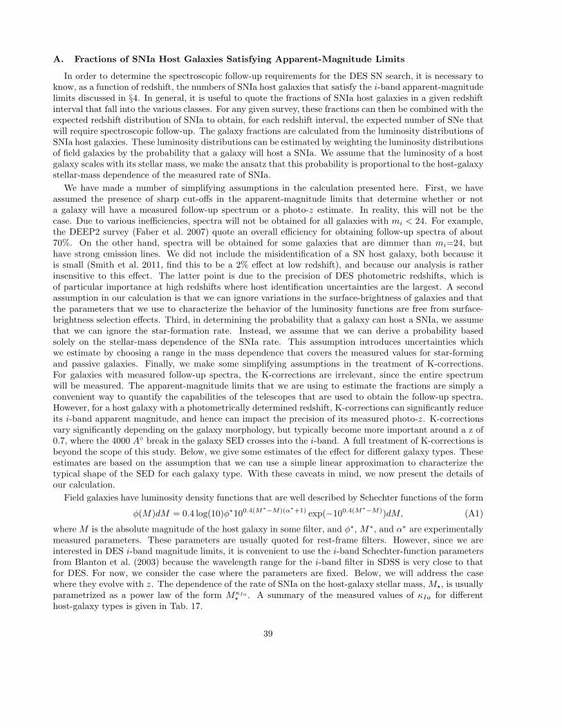
A. Fractions of SNIa Host Galaxies Satisfying Apparent-Magnitude Limits
In order to determine the spectroscopic follow-up requirements for the DES SN search, it is necessary toknow, as a function of redshift, the numbers of SNIa host galaxies that satisfy the i-band apparent-magnitudelimits discussed in §4. In general, it is useful to quote the fractions of SNIa host galaxies in a given redshiftinterval that fall into the various classes. For any given survey, these fractions can then be combined with theexpected redshift distribution of SNIa to obtain, for each redshift interval, the expected number of SNe thatwill require spectroscopic follow-up. The galaxy fractions are calculated from the luminosity distributions ofSNIa host galaxies. These luminosity distributions can be estimated by weighting the luminosity distributionsof field galaxies by the probability that a galaxy will host a SNIa. We assume that the luminosity of a hostgalaxy scales with its stellar mass, we make the ansatz that this probability is proportional to the host-galaxystellar-mass dependence of the measured rate of SNIa.
We have made a number of simplifying assumptions in the calculation presented here. First, we haveassumed the presence of sharp cut-offs in the apparent-magnitude limits that determine whether or nota galaxy will have a measured follow-up spectrum or a photo-z estimate. In reality, this will not be thecase. Due to various inefficiencies, spectra will not be obtained for all galaxies with mi < 24. For example,the DEEP2 survey (Faber et al. 2007) quote an overall efficiency for obtaining follow-up spectra of about70%. On the other hand, spectra will be obtained for some galaxies that are dimmer than mi=24, buthave strong emission lines. We did not include the misidentification of a SN host galaxy, both because itis small (Smith et al. 2011, find this to be a 2% effect at low redshift), and because our analysis is ratherinsensitive to this effect. The latter point is due to the precision of DES photometric redshifts, which isof particular importance at high redshifts where host identification uncertainties are the largest. A secondassumption in our calculation is that we can ignore variations in the surface-brightness of galaxies and thatthe parameters that we use to characterize the behavior of the luminosity functions are free from surface-brightness selection effects. Third, in determining the probability that a galaxy can host a SNIa, we assumethat we can ignore the star-formation rate. Instead, we assume that we can derive a probability basedsolely on the stellar-mass dependence of the SNIa rate. This assumption introduces uncertainties whichwe estimate by choosing a range in the mass dependence that covers the measured values for star-formingand passive galaxies. Finally, we make some simplifying assumptions in the treatment of K-corrections.For galaxies with measured follow-up spectra, the K-corrections are irrelevant, since the entire spectrumwill be measured. The apparent-magnitude limits that we are using to estimate the fractions are simply aconvenient way to quantify the capabilities of the telescopes that are used to obtain the follow-up spectra.However, for a host galaxy with a photometrically determined redshift, K-corrections can significantly reduceits i-band apparent magnitude, and hence can impact the precision of its measured photo-z. K-correctionsvary significantly depending on the galaxy morphology, but typically become more important around a z of0.7, where the 4000 A break in the galaxy SED crosses into the i-band. A full treatment of K-corrections isbeyond the scope of this study. Below, we give some estimates of the effect for different galaxy types. Theseestimates are based on the assumption that we can use a simple linear approximation to characterize thetypical shape of the SED for each galaxy type. With these caveats in mind, we now present the details ofour calculation.
Field galaxies have luminosity density functions that are well described by Schechter functions of the form
φ(M)dM = 0.4 log(10)φ∗100.4(M∗
−M)(α∗+1) exp(−100.4(M∗
−M))dM, (A1)
where M is the absolute magnitude of the host galaxy in some filter, and φ∗, M∗, and α∗ are experimentallymeasured parameters. These parameters are usually quoted for rest-frame filters. However, since we areinterested in DES i-band magnitude limits, it is convenient to use the i-band Schechter-function parametersfrom Blanton et al. (2003) because the wavelength range for the i-band filter in SDSS is very close to thatfor DES. For now, we consider the case where the parameters are fixed. Below, we will address the casewhere they evolve with z. The dependence of the rate of SNIa on the host-galaxy stellar mass, M⋆, is usuallyparametrized as a power law of the form MκIa
⋆ . A summary of the measured values of κIa for differenthost-galaxy types is given in Tab. 17.
39

Reference Host Galaxy Type κIa
Sullivan et al. (2006) Passive 1.10 ± 0.12Sullivan et al. (2006) Strongly Star Forming 0.74 ± 0.08Sullivan et al. (2006) Weakly Star Forming 0.66 ± 0.08Smith et al. (2011) Passive 0.67 ± 0.15Smith et al. (2011) Star-Forming 0.94 ± 0.08Li et al. (2011b) All 0.5
Table 17:: References for the dependence of the SNIa rate on the host-galaxy stellar mass.
The range of values in Tab. 17 exceeds the quoted uncertainties. Furthermore, Smith et al. (2011) andSullivan et al. (2006) disagree on the trend in values for a given type of host galaxy. We choose thereforeto take the lowest and highest values from Tab. 17 as the plausible range for the stellar-mass dependence ofSNIa hosts, and present fractions corresponding to this range. Assuming that the luminosity is proportionalto the stellar mass, we find that the luminosity density function for SNIa host galaxies is given by
φIa(M)dM = 0.4 log(10)φ∗
Ia100.4(M∗
−M)(α∗+κIa+1) exp(−100.4(M∗
−M))dM, (A2)
where φ∗
Ia is an (unknown) normalization constant that is assumed to be proportional to φ∗, and κIa = 0.5or 1.10. Eqn. A2 predicts an absolute-magnitude distribution of SNIa host galaxies that is in qualitativeagreement with the distribution measured by Yasuda & Fukugita (2010).
The next step is to determine, in the presence of an apparent magnitude cut, mlim, the number of SNIahost galaxies that will be seen in a thin shell at redshift z. All galaxies having absolute magnitudes brighterthan M = mlim − µ(z) − K(z) will be visible. Here, µ(z) is the distance modulus that is determined fromthe redshift assuming a particular cosmology, and K(z) is the K-correction that accounts for the redshift ofthe galaxy spectra. Hence the fraction of visible galaxies is given by
∫ mlim−µ(z)−K(z)
−∞φIa(M)dM
∫
∞
−∞φIa(M)dM
. (A3)
We note that the normalization constant, φ∗
Ia, in Eqn. A2 cancels in this fraction. Furthermore, for thevalues of α∗ that are typically measured from field-galaxy data, the integrals in Eqn. A3 are convergent forlarge M only because of the extra terms in the integrands that are dependent on κIa. Integrating Eqn. A3over M and z yields the fraction of visible galaxies in the range zlo < z < zhi.
f(zlo, zhi, mlim) =
∫ zhi
zloΓ(α∗ + κIa + 1, 100.4(M∗
−mlim−µ(z)−K(z)))dVco
Γ(α∗ + κIa + 1)∫ zhi
zlodVco
, (A4)
where Γ(s, x) and Γ(s) are the upper incomplete Gamma function and the Gamma function, respectively,and dVco is the co-moving volume element.
Given a cosmology, Eqn. A4 can now be evaluated over any desired redshift range to give the SNIa hostfractions. In Tab. 18, we present these fractions for a ΛCDM cosmology with ΩΛ = 0.73, Ωm = 0.27, H0 =72 km s−1 Mpc−1. We choose redshift intervals of 0.1 and the limiting cases of κIa=0.5 and κIa=1.1. We setK(z) = 0 for now. Two regions of the host-galaxy i-band apparent magnitude, mi, are considered: mi < 24,24 < mi < 26. These regions correspond to the current expectations for the apparent magnitude limits forwhich DES will be able to obtain spectroscopic and photo-z host-galaxy redshifts, respectively. SNIa whosehost galaxies do not fall into either of these two classes will either have no visible hosts, or have hosts withlarge uncertainties in their photo-z redshifts.
So far, we have assumed that the parameters characterizing the shape of the Schechter functions inEqns. A1 and A2 do not vary with redshift. In fact, current measurements indicate that the parameters φ∗,
40
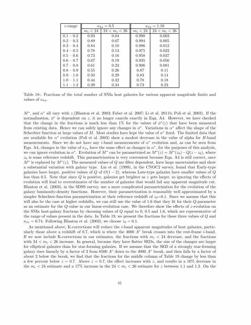
z-range κIa = 0.5 κIa = 1.10mi < 24 24 < mi < 26 mi < 24 24 < mi < 26
0.1 – 0.2 0.93 0.04 0.998 0.0020.2 – 0.3 0.89 0.07 0.994 0.0050.3 – 0.4 0.84 0.10 0.986 0.0120.4 – 0.5 0.78 0.13 0.975 0.0220.5 – 0.6 0.73 0.16 0.958 0.0370.6 – 0.7 0.67 0.19 0.935 0.0560.7 – 0.8 0.61 0.23 0.906 0.0810.8 – 0.9 0.55 0.26 0.87 0.110.9 – 1.0 0.50 0.29 0.83 0.141.0 – 1.1 0.44 0.32 0.78 0.181.1 – 1.2 0.39 0.34 0.73 0.23
Table 18:: Fractions of the total number of SNIa host galaxies for various apparent magnitude limits andvalues of κIa.
M∗, and α∗ all vary with z.(Blanton et al. 2003; Faber et al. 2007; Li et al. 2011b; Poli et al. 2003). If thenormalization, φ∗ is dependent on z, it no longer cancels exactly in Eqn. A4. However, we have checkedthat the change in the fractions is much less than 1% for the values of φ∗(z) that have been measuredfrom existing data. Hence we can safely ignore any changes in φ∗. Variations in α∗ affect the shape of theSchechter function at large values of M . Most studies have kept the value of α∗ fixed. The limited data thatare available for α∗ evolution (Poli et al. 2003) show a modest decrease in the value of alpha for B-bandmeasurements. Since we do not have any i-band measurements of α∗ evolution and, as can be seen fromEqn. A4, changes in the value of κIa have the same effect as changes in α∗, for the purposes of this analysis,we can ignore evolution in α∗. Evolution of M∗ can be parametrized as M∗(z) = M∗(z0)−Q(z− z0), wherez0 is some reference redshift. This parametrization is very convenient because Eqn. A4 is still correct, onceM∗ is replaced by M∗(z). The measured values of Q are filter dependent, have large uncertainties and showa substantial variation with galaxy type. Lin et al. (1999), in the CNOC2 survey, found that Early-typegalaxies have larger, positive values of Q of O(1 − 2), whereas Late-type galaxies have smaller values of Qless than 0.5. Note that since Q is positive, galaxies get brighter as z gets larger, so ignoring the effects ofevolution will lead to overestimates of the number of galaxies that would fail any apparent magnitude cut.Blanton et al. (2003), in the SDSS survey, use a more complicated parametrization for the evolution of thegalaxy luminosity-density functions. However, their parametrization is reasonably well approximated by asimpler Schechter-function parametrization at their reference redshift of z0=0.1. Since we assume that thiswill also be the case at higher redshifts, we can still use the value of 1.6 that they fit for their Q-parameteras an estimate for the Q-value in our linear-evolution case. We therefore show the effects of z-evolution onthe SNIa host-galaxy fractions by choosing values of Q equal to 0, 0.5 and 1.6, which are representative ofthe range of values present in the data. In Table 19, we present the fractions for these three values of Q andκIa = 0.74. Following Blanton et al. (2003), we choose z0 = 0.1.
As mentioned above, K-corrections will reduce the i-band apparent magnitudes of host galaxies, partic-ularly those above a redshift of 0.7, which is where the 4000 A break crosses into the rest-frame i-band.If we now include K-corrections in our estimates, the fractions with mi < 24 decrease, and the fractionswith 24 < mi < 26 increase. In general, because they have flatter SEDs, the size of the changes are largerfor elliptical galaxies than for star-forming galaxies. If we assume that the SED of a strongly star-forminggalaxy rises linearly by a factor of 3 from 8500 A down to the 4000 A break, and then falls by a factor ofabout 2 below the break, we find that the fractions for the middle column of Table 19 change by less thana few percent below z = 0.7. Above z = 0.7, the effect increases with z, and results in a 16% decrease inthe mi < 24 estimate and a 17% increase in the 24 < mi < 26 estimate for z between 1.1 and 1.2. On the
41

z-range Q = 0 Q = 0.5 Q = 1.6mi < 24 24 < mi < 26 mi < 24 24 < mi < 26 mi < 24 24 < mi < 26
0.1 – 0.2 0.98 0.01 0.98 0.01 0.99 0.010.2 – 0.3 0.96 0.03 0.97 0.03 0.97 0.020.3 – 0.4 0.94 0.05 0.94 0.04 0.95 0.040.4 – 0.5 0.91 0.07 0.92 0.06 0.94 0.050.5 – 0.6 0.87 0.10 0.89 0.09 0.92 0.060.6 – 0.7 0.82 0.13 0.85 0.11 0.90 0.070.7 – 0.8 0.77 0.17 0.82 0.14 0.89 0.090.8 – 0.9 0.72 0.20 0.78 0.16 0.87 0.100.9 – 1.0 0.67 0.24 0.74 0.19 0.86 0.101.0 – 1.1 0.61 0.28 0.70 0.22 0.85 0.111.1 – 1.2 0.55 0.32 0.67 0.24 0.84 0.12
Table 19:: Fractions of the total number of SNIa host galaxies for various apparent magnitude limits forκIa = 0.74 and three values of M∗-evolution parameter, Q. The chosen values of Q span the range of possiblevalues found in the field-galaxy data.
other hand, if we assume that the SED of an elliptical galaxy is flat and falls by a factor of 2 below the 4000A break, we find that the effects are much larger. Even below z = 0.7, the changes grow with z, up to a10% decrease in the mi < 24 estimate and a 6% increase in the 24 < mi < 26 estimate for z between 0.6and 0.7. Above z = 0.7, the effect of the corrections again rises with z and results in a 40% decrease in themi < 24 estimate and a 24% increase in the 24 < mi < 26 estimate for z between 1.1 and 1.2. The effect ofK-corrections on the galaxy fractions should lie somewhere between these two extremes, depending on theprecise mix of SNIa host-galaxy morphologies. Hence, the size of this uncertainty is comparable to the otheruncertainties discussed in this section. Note, however, that these uncertainties affect only the estimates ofthe size of the photo-z sample. We have seen in §8.1, that the FOM decreases by only about 15 units, evenif no SNe in the photo-z sample are included. Hence, adding some fraction of SNe from the photo-z sampleto the analysis can result in only very modest gains in the FOM, and we expect that our forecasts for theFOM values to be largely unaffected by the uncertainties in the K-corrections.
We conclude that uncertainties in the data that can be used to constrain the SNIa host-galaxy fractionsare large and lead to big variations in the estimates of the number of host galaxies that fall into the variousmagnitude classes. As discussed above, we have made several simplifying assumptions in our calculations thatignore a number of known effects due to inefficiencies in redshift determinations, galaxy morphology, galaxysurface brightness and star-formation rate. We have attempted to include the effects due to z-evolution ofthe Schechter functions, but here too there are dependencies on galaxy morphology that contribute to theuncertainties on the fractions. We quote numbers in the mid-range of the predictions in the body of thepaper, but note that predictions at high z vary by about 25%.
B. SNe systematic uncertainties in the FoM calculation
The use of a Fisher Information Matrix in forecasting constraints from a survey has been discussed inseveral works. While the general formalism can account for certain kinds of systematic uncertainties in theforecasted constraints, the specific examples for supernova surveys that are usually studied only account forstatistical uncertainties. The DETF report suggested accounting for systematic uncertainties in forecastingcosmological constraints from supernova surveys. In particular, the DETF report discussed four kinds ofsystematic uncertainties: 1. photo-z errors, 2. absolute magnitude uncertainties, 3. step µ offset for thenear sample, 4. quadratic µ offset (see subsection below for additional information). With the advantage ofour simulations and knowledge specific to the setup of DES, we extend the DETF analysis by choosing a
42

more appropriate set of systematics particularly with respect to their fourth systematic parameter. In thisappendix, we explain the choices made in our paper and how they relate to the DETF choices.
The basic idea is that the naive estimator for the distance modulus as obtained from the light curvefitter is biased when the survey setup and conditions or the properties of SNIa are actually different fromthose assumed in the analysis. However, since the survey conditions can be varied in our simulation inputs,we can estimate the bias ∆µ(z, Θ), which is the expected deviation of the estimated distance modulusfrom the true distance modulus, for each set of conditions. We thus correct for the bias by replacingµ(z, θc) → 〈(µ, zΘ)〉 = µ(z, θc) − ∆µ(z, Θ), where Θ includes not only the cosmological parameters, θc,but also the set of systematic parameters, θn, modeling the setup and SN properties. These systematicparameters are measured independently, and the information from these measurements may be treated as aGaussian prior resulting in a prior Fisher matrix Find. Extending the set of model parameters Θ to includethese systematic parameters θn as “nuisance parameters”, we can use the replacement in computing theFisher matrix and then marginalize over the allowed values of these nuisance parameters. We give theexpression for the Fisher matrix
Ftot = Fij + FStage II + Find,
Fij(Θp) =∂〈µa(z, Θ)〉
∂Θi
∣
∣
∣
∣
Θp
(Cov−1)ab
∂〈µb(z, Θ)〉∂Θj
∣
∣
∣
∣
Θp
+1
2
∂2 ln(det(Cov))
∂Θi∂Θj
(B1)
where a, b index the SN and are summed over in the above equation, and Cov is the covariance matrixused in the (statistics only) Fisher matrix. The second term arises from the derivatives of the logarithmof the normalization of the Gaussian. The normalization of the Gaussian distribution only depends oncosmological parameters through the term ∂µ
∂zδz added in quadrature to the light curve fit errors. For the
cases where supernova redshifts are determined spectroscopically leading to small δz, the covariance matrixCov becomes independent of the cosmological parameters and hence the second term is zero. For cases,where the supernova redshift is determined photometrically, this turns out to be a very small contribution.All partial derivatives are evaluated at a set of fiducial parameters Θp taken to be the DETF parametersΩDE , w0, wa, Ωk = 0.73,−1, 0, 0 for the cosmological parameters, and our best estimates for the nuisanceparameters. We note that this is exactly the idea behind the treatment suggested in the DETF report. Wenow proceed to discuss our choice for the set of nuisance parameters as described below.
B.1. Nuisance Parameters
The main differences in our method, compared to that presented in the DETF report, are as follows:
1. We have an improved estimate of the effect of photo-z uncertainties, coming from the full simulationof the DES survey.
2. The uncertainty in absolute magnitudes referred to in the DETF report is analytically marginalizedin our likelihood function. Therefore, our “statistics only” Fisher matrix accounts for this in thecorrelated covariance matrix.
3. In our SN analysis, we include two low-redshift samples as anchors: the 3-year SDSS sample with∼350 SNe and a sample of 300 supernovae taken to be at redshift of 0.055 (Li et al. 2011a), eachwith a Gaussian error of 0.13 magnitudes . Neither of these samples were included in the calculationof the Stage II prior Fisher matrix. In each of these low-redshift samples, the dominant systematicuncertainty is expected to be a step µ offset of the kind described in the DETF report. Therefore, weinclude a step offset for each of the low-redshift samples. We also assume a Gaussian prior on eachof these step offsets of width δMlowz = δMSDSS = 0.01. This is consistent with the suggestion of theDETF report.
4. In the DETF report, all other systematic effects were treated as an effective linear and quadratic shift inµ(z). The relevant nuisance parameters were taken to be the first and second order redshift coefficients.
43

We have used a more realistic estimate of the effects of systematics on µ(z). In our simulations, wevary the systematic parameters θn, which model the instrumental setup and supernova properties, fromtheir assumed values and study how the µobs(z) changes. Assuming that we are in the linear regime,we write
µobs(z, Θ) = µobs(z, Θp) +∑
j
∂µobs(z, Θ)
∂θjn
∣
∣
∣
∣
Θp
∆θjn (B2)
where the sum runs over j which indexes the list of systematic parameters θn.
By varying each systematic parameter under consideration, one at a time, in our simulations, we estimate
the average values of the partial derivatives ∂µobs(z,Θ)
∂θjn
in redshift bins of 0.1 in terms of fitting functions
that involves 3 to 6 parameters. Using these, we evaluate the Fisher matrix in the parameter space Θ whichincludes both the cosmological parameters θc and the systematic parameters θn. The parameters θn willbe set or measured to a fiducial value with an estimated uncertainty either in the process of calibration(parameters related to survey conditions) or by other experiments (SNIa light curve model parameters orSNcc fractions). These measurements allow us to use appropriate priors on the deviation of these parametersfrom their fiducial values. Therefore we will marginalize over all the systematic parameters with such priorson each of them. We now proceed to discuss the relevant set of systematic parameters.
We first identify the relevant set of systematic effects and parametrize them. These are the zero-pointsin each filter band, the wavelength of the centroid of the filters, the fraction of SNe which are SNcc butmisidentified as SNIa, and the values of τAV
and RV. First, we describe these parameters, and the priors onthem due to independent measurements.
Zero-Points: We include the deviation in zero-points in each band g0, r0, i0, z0 from the fiducial valuesas parameters. Further, we expect to be able to calibrate these independently to an error of 0.01 magnitudes.Hence we assume a Gaussian prior on each of these parameters with a width σg
zpt = σrzpt = σi
zpt = σzzpt = 0.01.
Wavelength of Filter Centroid: We include the deviation of the wavelength λg, λr, λi, λz of the centroidof each filter from the fiducial values. Further, we expect to be able to calibrate these independently toan error of 10 angstroms. Hence we assume a Gaussian prior on each of these parameters with a widthσg
λ = σrλ = σi
λ = σzλ = 10 A.
Core-Collapse Fraction: The sample purity for the hybrid 10-field survey is 98%. We are taking theuncertainty in this value to be 2%, and have shown that the effect on the FoM is still smaller than the otheruncertainties. To be specific, we use fcc = 0 as a fiducial value and σfcc
= 0.02 as the Gaussian uncertaintyin fcc.
CCM Dust Model Parameters: µfit depends on the true values of the parameters τAVand RV values.
Our simulations are based on SDSS results (Kessler et al. 2009a) and, hence, we assume fiducial values ofτAV
=0.334 and RV=2.18. Assuming that these variables are correlated in the way determined by the SDSSSN survey (Kessler et al. 2009a), we expect to have independent measurements determining these parametersas a correlated Gaussian with a covariance matrix C with CRVRV
= 0.1444, CτAV,τAV
= 0.003136, CτAVRV
=0.0036176.
As described in §2, these parameters are inputs to our simulations. Therefore, we can study changes inthe fitted values of µ by changing these input parameters in SNANA. For each of the parameters that we
shall describe, we compute∂µeff (z,Θ)
∂Θi|Θp
by numerically evaluating the partial derivative of µeff (z, Θ) asa function of redshift. For doing so, µeff (z, Θ) is estimated as the sample mean of obtained values of thefitted distance modulus µfit in redshift bins of 0.1. Having obtained these estimated values, along theirdispersions, we fit these values at discrete redshifts bin centroids to simple functions of the redshift. Thisallows us to evaluate the partial derivative at any redshift in the range of observation (0, 1.2).
44

REFERENCES
Abell, P. A. et al. 2009, e-prints arXiv:0912.0201
Albrecht, A. et al. 2006, e-prints arXiv:astro-ph/0609591
Amanullah, R. et al. 2010, ApJ, 716, 712
Astier, P. et al. 2006, A&A, 447, 31
Bazin, G. et al. 2009, A&A, 499, 653
Bessell, M. S. 1990, PASP, 102, 1181
Blanton, M. R. et al. 2003, ApJ, 592, 819
Burns, C. R. et al. 2011, AJ, 141, 19
Cardelli, J. A., Clayton, G. C., & Mathis, J. S.1989, ApJ, 345, 245
Chevallier, M. & Polarski, D. 2001, InternationalJournal of Modern Physics D, 10, 213
Conley, A. et al. 2011, ApJS, 192, 1
Dawson, K. S. et al. 2009, AJ, 138, 1271
Diehl, H. T. et al. 2008, in Society of Photo-Optical Instrumentation Engineers (SPIE)Conference Series, Vol. 7021
Dilday, B. et al. 2008, ApJ, 682, 262
Emerson, J. P. et al. 2004, The Messenger, 117, 27
Estrada, J. et al. 2010, in Society of Photo-OpticalInstrumentation Engineers (SPIE) ConferenceSeries, Vol. 7735
Faber, S. M. et al. 2007, ApJ, 665, 265
Flaugher, B. L. et al. 2010, in Society of Photo-Optical Instrumentation Engineers (SPIE)Conference Series, Vol. 7735
Foley, R. J. et al. 2009, AJ, 137, 3731
Freedman, W. L. et al. 2009, ApJ, 704, 1036
Frieman, J. A., Turner, M. S., & Huterer, D.2008a, ARA&A, 46, 385
Frieman, J. A. et al. 2008b, AJ, 135, 338
Groom, D. E. et al. 2006, in Bulletin of the Amer-ican Astronomical Society, Vol. 38, Bulletin ofthe American Astronomical Society, 1038
Guy, J. et al. 2007, A&A, 466, 11
Hamuy, M. et al. 2006, PASP, 118, 2
Holland, S. 2002, Experimental Astronomy, 14, 83
James, F. 1994, CERN Program Library LongWriteup D506
Jarvis, M. J. 2009, e-prints arXiv:0909.3945
Jha, S., Riess, A. G., & Kirshner, R. P. 2007, ApJ,659, 122
Kessler, R. et al. 2009a, ApJS, 185, 32
—. 2009b, PASP, 121, 1028
—. 2010a, ApJ, 717, 40
—. 2010b, PASP, 122, 1415
Leaman, J., Li, W., Chornock, R., & Filippenko,A. V. 2011, MNRAS, 412, 1419
Lewis, P. M., Rogers, H., & Schindler, R. H.2010, in Society of Photo-Optical Instrumenta-tion Engineers (SPIE) Conference Series, Vol.7735
Li, W. et al. 2007, ApJ, 661, 1013
—. 2011a, MNRAS, 412, 1441
—. 2011b, MNRAS, 412, 1473
Lin, H. et al. 1999, ApJ, 518, 533
Linder, E. V. 2003, Physical Review Letters, 90,091301
Marriner, J. et al. 2011, ApJ, submitted
Melinder, J. et al. 2011, A&A, 532, A29
Miknaitis, G. et al. 2007, ApJ, 666, 674
Nugent, P., Kim, A., & Perlmutter, S. 2002,PASP, 114, 803
Oyaizu, H. et al. 2008, ApJ, 689, 709
Perlmutter, S. et al. 1999, ApJ, 517, 565
Poli, F. et al. 2003, ApJ, 593, L1
Prieto, J. L., Stanek, K. Z., & Beacom, J. F. 2008,ApJ, 673, 999
45

Regnault, N. et al. 2009, A&A, 506, 999
Richardson, D. et al. 2002, AJ, 123, 745
Riess, A. G. et al. 1998, AJ, 116, 1009
Sako, M. et al. 2011, ApJ, 738, 162
Schlegel, D. J., Finkbeiner, D. P., & Davis, M.1998, ApJ, 500, 525
Scolnic, D. M. et al. 2009, ApJ, 706, 94
Smartt, S. J. et al. 2009, MNRAS, 395, 1409
Smith, M. et al. 2011, e-print arXiv:1108.4923
Stritzinger, M. D. et al. 2011, AJ, 142, 156
Strolger, L.-G. et al. 2004, ApJ, 613, 200
Sullivan, M. et al. 2006, ApJ, 648, 868
—. 2011, ApJ, 737, 102
van den Bergh, S., Li, W., & Filippenko, A. V.2005, PASP, 117, 773
Weinberg, D. H. et al. 2012, e-prints arXiv:astro-ph/1201.2434
Yasuda, N. & Fukugita, M. 2010, AJ, 139, 39
This 2-column preprint was prepared with the AAS LATEXmacros v5.0.
46