supply chain network capacity competition with outsourcing
TRANSCRIPT

Supply Chain Network Capacity Competition withOutsourcing: A Variational Equilibrium Framework
Anna Nagurney 1, Min Yu 2 and Deniz Besik 3
1,3 Department of Operations and Information ManagementIsenberg School of ManagementUniversity of Massachusetts
Amherst, MA 010032 Pamplin School of Business Administration
University of PortlandUniversity of MassachusettsPortland, Oregon 97203
POMS 28th Annual Conference in Seattle, WAMay 5-8, 2017
Nagurney, Yu and Besik (UMass) Supply Chain Network Capacity Competition NEDSI

This presentation is based on the paper:
Nagurney, A., Yu, M. and Besik, D., 2017. Supply Chain Network CapacityCompetition with Outsourcing: A Variational Equilibrium Framework. In press inthe Journal of Global Optimization.
Nagurney, Yu and Besik (UMass) Supply Chain Network Capacity Competition NEDSI

Background and Motivation
The logistics landscape, from warehousing to distribution, underpinningsupply chains is dealing with increased competition and tightenedcapacity along with increasing consolidation.
29% of shippers in a recent survey noting that they have engaged with alarger number of third party logistics providers to get access to gaincapacity.
73% of shippers noted that they increased their use of outsourced logisticsservices in 2015, as compared to a figure of 68% in the previous year.
Nagurney, Yu and Besik (UMass) Supply Chain Network Capacity Competition NEDSI

Background and Motivation
Firms compete for shared capacities of third party logistics providers forboth distribution center space as well as freight service provision to theirdemand markets.
UPS has recently built several healthcare logistics hubs in Asia and thePacific in order to catch up with the rapid growth in the demand forpharmaceuticals.
Nestle and PepsiCo, are sharing warehouse capabilities, in the form ofstorage, packing operations in Belgium and Luxembourg.
Kimberly-Clark Corporation has been very innovative in sharingwarehouses as well as freight service provision with multiple differentcompanies, including Unilever and Kellogg, in several European countrieswith results of cost reduction and improvement in customer service.
Nagurney, Yu and Besik (UMass) Supply Chain Network Capacity Competition NEDSI

Background and Motivation
We develop a competitive supply chain network model consisting ofmultiple firms involved in the manufacture/production of a similar,substitutable, product distinguished by each firm’s brand.
The firms have available manufacturing plants and distribution centers, andsupply the same demand points, which can correspond to retailers.
The firms may avail themselves of external distribution centers, to whichthey can outsource any or all of the storage of their products and also theultimate delivery to the demand markets.
The external distribution center storage links and freight service provisionlinks have associated capacities and the firms compete for storage andfreight service provision.
Nagurney, Yu and Besik (UMass) Supply Chain Network Capacity Competition NEDSI
Generalized Nash Equilibrium
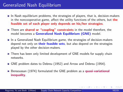
In Nash equilibrium problems, the strategies of players, that is, decision-makersin the noncooperative game, affect the utility functions of the others, but thefeasible set of each player only depends on his/her strategies.
There are shared or “coupling” constraints in the model therefore, themodel becomes a Generalized Nash Equilibrium (GNE) model.
In a Generalized Nash Equilibrium game, the strategies of decision-makersdepend not only on their feasible sets, but also depend on the strategiesplayed by the other decision-makers.
There has been only limited development of GNE models for supply chainnetworks.
GNE problem dates to Debreu (1952) and Arrow and Debreu (1954).
Bensoussan (1974) formulated the GNE problem as a quasi-variationalinequality.
Nagurney, Yu and Besik (UMass) Supply Chain Network Capacity Competition NEDSI

Some Literature on GNE
Nagurney, Alvarez Flores, and Soylu (2016) focused on post-disasterhumanitarian relief and constructed an integrated network model in whichdisaster relief NGOs compete for financial funds from donors while alsoderiving utility from providing relief through their supply chains tomultiple points of demand.
The shared constraints consist of lower and upper bounds for relief suppliesat demand points in order to ensure that needs of the victims are met butnot at the expense of material convergence and oversupply.
The GNE model in Nagurney, Alvarez Flores, and Soylu (2016) was of astructure that enabled its reformulation as an optimization problem.
Here, we make use of a variational equilibrium (cf. Facchinei and Kanzow(2010), Kulkarni and Shanbhag (2012)), which is a specific kind of GNE.
GNE models have been constructed for the energy and airline industry(see, e.g., Contreras, Klusch, and Krawczyk (2004), Jiang and Pang (2011)).
Nagurney, Yu and Besik (UMass) Supply Chain Network Capacity Competition NEDSI

The Network Topology
The I firms compete noncooperatively in an oligopolistic manner.
Firms compete for and may share space in the nOD external distribution centers, and the sameholds for the subsequent freight service provision for distribution to the nR demand markets.
mR1mR2 · · · mRnR
XXXXXXXXXXXXz
hhhhhhhhhhhhhhhhhh
hhhhhhhhhhhhhhhhhhhhhhhhhhhhh
HHHH
HHj
XXXXXXXXXXXXz
hhhhhhhhhhhhhhhhhhhhhhhh
((((((((((((((((((((((((
((((((((((((((((((
����
���
(((((((((((((((((((((((((((((
((((((((((((((((((((((((
������������9
������� ?
XXXXXXXXXXXXz
������������9
����
���
HHHH
HHj
mD11,2 · · · mD1
n1D ,2mD I
1,2 · · · mD InID ,2
mOD1,2 · · · mODnOD ,2
? ? ? ?? ?
· · · · · ·mD1
1,1 · · · mD1n1D ,1
mD I1,1 · · · mD I
nID ,1mOD1,1 · · · mODnOD ,1
?
ZZZZZZ~
XXXXXXXXXXXXXXXXXXz
````````````````````````
���
���= ?
aaaaaaaaaaaa
XXXXXXXXXXXXXXXXXXz ?
ZZZZZZ~
������������������9
!!!!!!!!!!!!
��
��
��= ?
������������������9
M11m · · · mM1
n1MM I
1m · · · mM I
nIM
�������
AAAAAAU
�������
AAAAAAU
m1 mI· · ·Firm 1
Manufacturing/Production
Firm I
Transportation
StorageStorage Storage
Distribution Distribution
· · ·
Nagurney, Yu and Besik (UMass) Supply Chain Network Capacity Competition NEDSI

The Supply Chain Problem with Capacity Competition
DemandThe following conservation of flow equations must hold for each firm i : i = 1, . . . , I :∑
p∈P ik
x ip = dik , ∀k, (1)
Nonnegativity constraint of the path flows
The path flows must be nonnegative; that is, for each firm i ; i = 1, . . . , I :
x ip ≥ 0, ∀p ∈ P i . (2)
Link flowsThe expression that relates the link flows of each firm i ; i = 1, . . . , I , to the path flows isgiven by:
f ia =∑p∈P
x ipδap, ∀a ∈ L, (3)
where δap = 1, if link a is contained in path p, and 0, otherwise.
Nagurney, Yu and Besik (UMass) Supply Chain Network Capacity Competition NEDSI

The Supply Chain Problem with Capacity Competition
Capacity of the individual links of the firms:
For links corresponding to the individual firm networks Li ; i = 1, . . . , I , we must have that:
f ia ≤ uia, ∀a ∈ Li . (4)
Capacity of the outsourced links:
For the links corresponding to the outsourced storage and distribution, the followingcapacity constraints must be satisfied:
I∑i=1
f ia ≤ ua, ∀a ∈ LS . (5)
Demand Price
We may express the demand price function, ρik(d), as:
ρik = ρik(x) ≡ ρik(d), ∀i , ∀k. (6)
Nagurney, Yu and Besik (UMass) Supply Chain Network Capacity Competition NEDSI

The Supply Chain Problem with Capacity Competition
Link costThe total operational cost associated with link a, ∀a ∈ L and all firms i;i=1,. . . ,I, that is:
c ia = c ia(f ), ∀a ∈ L, (6)
Profit/Utility
The profit/utility function of farm i , denoted by Ui , is given by:
Ui =
nR∑k=1
ρik(d)dik −∑
a∈Li∪LS
c ia(f ), (7)
Vector of Strategies
Xi is the vector of path flows associated with firm i , that is:
Xi ≡ {{xp}|p ∈ P i} ∈ RnPi
+ . (8)
Profits of all the firms
We group the profits of all the firms into an I -dimensional vector U, where
U = U(X ). (9)
Nagurney, Yu and Besik (UMass) Supply Chain Network Capacity Competition NEDSI

The Supply Chain Problem with Capacity Competition
Capacity in path flows
In view of the conservation of flow equations (3), we may rewrite the individual firms’capacity constraints (4) in terms of path flows as:∑
p∈P
x ipδap ≤ uia, ∀a ∈ Li ,∀i . (10)
Capacity of outsourced in path flows
We may rewrite the shared capacity constraints (5) in terms of path flows such that:
I∑i=1
∑p∈P
x ipδap ≤ ua, ∀a ∈ LS . (11)
Feasible sets of the different constraintsEach firm i has individual feasible set Ki for i = 1, . . . , I , as:
Ki ≡ {x ip ≥ 0,∀p ∈ P i and (10) holds}. (12)
The feasible set consisting of the shared constraints, S, can be defined as:
S ≡ {x |(11) holds}. (13)
Nagurney, Yu and Besik (UMass) Supply Chain Network Capacity Competition NEDSI

The Supply Chain Problem with Capacity Competition
Definition 1: Supply Chain Network Generalized Nash Equilibrium withCapacity Competition and OutsourcingA path flow pattern X ∗ ∈ K =
∏Ii=1 Ki , X
∗ ∈ S, constitutes a supply chainnetwork Generalized Nash Equilibrium if for each firm i ; i = 1, . . . , I :
Ui (X∗i , X
∗i ) ≥ Ui (Xi , X
∗i ), ∀Xi ∈ Ki ,∀X ∈ S, (14)
where X ∗i ≡ (X ∗1 , . . . ,X∗i−1,X
∗i+1, . . . ,X
∗I ).
An equilibrium is established if no firm can unilaterally improve its profit bychanging its product flows in the supply chain network, given the productflow decisions of the other firms, and subject to the capacity constraints,both individual and shared/coupling ones.
Nagurney, Yu and Besik (UMass) Supply Chain Network Capacity Competition NEDSI

The Supply Chain Problem with Capacity Competition
If there are no coupling, that is, shared, constraints in the above model, thenX and X ∗ in Definition 1 need only lie in the set K .
The solution to what would then be a Nash equilibrium problem (see Nash (1950,1951)) would coincide with the solution of the following variational inequalityproblem: determine X ∗ ∈ K , such that
−I∑
i=1
〈∇Xi Ui (X∗),Xi − X ∗i 〉 ≥ 0, ∀X ∈ K . (15)
The strategies of the “players,” affect not only the values of the others’objective functions, but also the strategies of the firms affect the otherfirms’ strategies because of the shared constraints.
Nagurney, Yu and Besik (UMass) Supply Chain Network Capacity Competition NEDSI

Variational Equilibrium
In a GNE defined by a variational equilibrium, the Lagrange multipliers associatedwith the coupling constraints are all the same.
Definition 2: Variational EquilibriumA strategy vector X ∗ is said to be a variational equilibrium of the aboveGeneralized Nash Equilibrium game if X ∗ ∈ K ,X ∗ ∈ S is a solution of thevariational inequality:
−I∑
i=1
〈∇Xi Ui (X∗),Xi − X ∗i 〉 ≥ 0, ∀X ∈ K ,∀X ∈ S. (16)
Nagurney, Yu and Besik (UMass) Supply Chain Network Capacity Competition NEDSI

Expansion of Variational Inequality
Specifically, by definition, we have that
−∇Xi Ui (X ) =
[−∂Ui
∂x ip; p ∈ P i
k ; k = 1, . . . , nR
]. (17)
We also know that, in view of (1) and (7), for paths p ∈ P ik :
−∂Ui
∂x ip= −
∂(∑nR
l=1 ρil(d)∑
q∈P ilx iq −
∑b∈Li∪LS c ib(f ))
∂x ip. (18)
Making use of (1) and (3) and the expressions:
∂C ip(x)
∂x ip≡
∑a∈Li∪Ls
∑b∈Li∪Ls
∂c ib(f )
∂f iaδap, (19a)
∂ρil(x)
∂x ip≡ ∂ρil(d)
∂dik. (19b)
we obtain:
−∂Ui
∂x ip=
∂C ip(x)
∂x ip− ρik(x)−
nR∑l=1
∂ρil(x)
∂x ip
∑q∈P i
l
x iq
. (20)
Nagurney, Yu and Besik (UMass) Supply Chain Network Capacity Competition NEDSI
Expansion of Variational Inequality
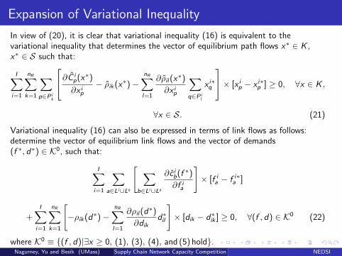
In view of (20), it is clear that variational inequality (16) is equivalent to thevariational inequality that determines the vector of equilibrium path flows x∗ ∈ K ,x∗ ∈ S such that:
I∑i=1
nR∑k=1
∑p∈P i
k
∂C ip(x∗)
∂x ip− ρik(x∗)−
nR∑l=1
∂ρil(x∗)
∂x ip
∑q∈P i
l
x i∗q
× [x ip − x i∗p ] ≥ 0, ∀x ∈ K ,
∀x ∈ S. (21)
Variational inequality (16) can also be expressed in terms of link flows as follows:determine the vector of equilibrium link flows and the vector of demands(f ∗, d∗) ∈ K0, such that:
I∑i=1
∑a∈Li∪Ls
[ ∑b∈Li∪Ls
∂c ib(f ∗)
∂f ia
]× [f ia − f i∗a ]
+I∑
i=1
nR∑k=1
[−ρik(d∗)−
nR∑l=1
∂ρil(d∗)
∂dikd∗il
]× [dik − d∗ik ] ≥ 0, ∀(f , d) ∈ K0 (22)
where K0 ≡ {(f , d)|∃x ≥ 0, (1), (3), (4), and (5) hold}.Nagurney, Yu and Besik (UMass) Supply Chain Network Capacity Competition NEDSI

Alternative Variational Inequality Formulations
Theorem 1: Alternative Variational Inequality Formulations of the VariationalEquilibrium in Path Flows and in Link FlowsThe variational equilibrium (16) is equivalent to the variational inequality: determinethe vector of equilibrium path flows, and the vector of optimal Lagrange multipliers,(x∗, λ∗, η∗) ∈ K, such that:
I∑i=1
nR∑k=1
∑p∈P i
k
∂C ip(x∗)
∂x ip+∑a∈Li
λ∗aδap +∑a∈LS
η∗a δap − ρik(x∗)−nR∑l=1
∂ρil(x∗)
∂x ip
∑q∈P i
l
x i∗q
×[x ip − x i∗p ] +I∑
i=1
∑a∈Li
uia −∑p∈P
x i∗p δap
× [λa − λ∗a ]
+∑a∈LS
ua − I∑i=1
∑p∈P
x i∗p δap
× [ηa − η∗a ] ≥ 0, (x , λ, η) ∈ K, (23)
where K ≡ {(x , λ, η)|x ∈ RnP+ , λ ∈ R
∑Ii=1 nLi
+ , η ∈ RnLS
+ }.
Nagurney, Yu and Besik (UMass) Supply Chain Network Capacity Competition NEDSI

Alternative Variational Inequality Formulations
The variational inequality (23), in turn, can be rewritten in terms of link flows as:determine the vector of equilibrium link flows, the vector of demands, and the vectorof optimal Lagrange multipliers, (f ∗, d∗, λ∗, η∗) ∈ K1, such that:
I∑i=1
∑a∈Li
[∑b∈Li
∂c ib(f ∗)
∂f ia+ λ∗a
]× [f ia − f i∗a ] +
I∑i=1
∑a∈LS
∑b∈LS
∂c ib(f ∗)
∂f ia+ η∗a
× [f ia − f i∗a ]
+I∑
i=1
nR∑k=1
[−ρik(d∗)−
nR∑l=1
∂ρil(d∗)
∂dikd∗il
]× [dik − d∗ik ]
+I∑
i=1
∑a∈Li
[uia − f i∗a
]×[λa−λ∗a ]+
∑a∈LS
[ua −
I∑i=1
f i∗a
]×[ηa−η∗a ] ≥ 0, (f , d , λ, η) ∈ K1,
(24)where K1 ≡ {(f , d , λ, η)|∃x ≥ 0, (1) and (3) hold, andλ ≥ 0, η ≥ 0}.
Proof: Variational inequality (23) follows from the Karush Kuhn Tucker conditions(see also Lemma 1.2 in Yashtini and Malek (2007)). Variational inequality (24) thenfollows from variational inequality (23) by making use of the conservation of flowequations. 2Nagurney, Yu and Besik (UMass) Supply Chain Network Capacity Competition NEDSI

Special Cases of the Supply Chain Network OligopolyModel: No Shared Constraints
����R1 · · · RnR ����HHH
HHHHHj
PPPPPPPPPPPq?
�����������) ?
������
���
D11,2 ����· · · ����D1
n1D ,2D I
1,2 ����· · · ����D InID ,2
? ? ? ?
· · ·
D11,1 ����· · · ����D1
n1D ,1D I
1,1 ����· · · ����D InID ,1
?
HHHHHH
HHj?
������
��� ?
HHHHHH
HHj?
������
���
· · ·
M11 ����· · · ����M1
n1MM I
1 ����· · · ����M InIM
��
��
@@@@R
��
��
@@@@R
����1 ����I· · ·
Firm 1
Manufacturing/Production
Transportation
Storage
Distribution
Firm I
Nagurney, Yu and Besik (UMass) Supply Chain Network Capacity Competition NEDSI

Special Cases of the Supply Chain Network OligopolyModel: Outsource Storage and Freight Services
mR1mR2 · · · mRnR
������� ?
XXXXXXXXXXXXz
������������9
�������
HHHHHHj
mOD1,2 · · · mODnOD ,2
? ?
mOD1,1 · · · mODnOD ,1
XXXXXXXXXXXXXXXXXXz
````````````````````````
aaaaaaaaaaaa
XXXXXXXXXXXXXXXXXXz
������������������9
!!!!!!!!!!!!
������������������9
M11m · · · mM1
n1MM I
1m · · · mM I
nIM
�������
AAAAAAU
�������
AAAAAAU
m1 mI· · ·Firm 1
Manufacturing/Production
Firm I
Transportation
Storage
Distribution
· · ·
Nagurney, Yu and Besik (UMass) Supply Chain Network Capacity Competition NEDSI

The Algorithm - Euler Method
Euler method, which is induced by the general iterative scheme of Dupuis andNagurney (1993) is a solution methodology of the Variational Inequality Problem.Specifically, iteration τ of the Euler method is given by:
X τ+1 = PK(X τ − aτF (X τ )), (25)
The Euler method, the sequence {aτ} must satisfy:∑∞τ=0 aτ =∞, aτ > 0,
aτ → 0, as τ →∞.
Nagurney, Yu and Besik (UMass) Supply Chain Network Capacity Competition NEDSI

The Euler Method Explicit Formulae
For each path p ∈ P ij , ∀i , j , compute:
x iτ+1
p = max{0, x iτ
p + aτ (ρik (xτ ) +
nR∑l=1
∂ρil (xτ )
∂x ip
∑q∈P i
l
x iτ
q −∂C i
p(xτ )
∂x ip−
∑a∈Li
λτa δap −∑a∈LS
ητa δap)},
∀p ∈ P ik ; i = 1, . . . , I ; k = 1, . . . , nR . (26)
The Lagrange multipliers for each link a ∈ Li ; i = 1, . . . , I , compute:
λτ+1a = max{0, λτa + aτ (
∑p∈P
x iτ
p δap − uia)}, ∀a ∈ Li ; i = 1, . . . , I . (27)
The computation process for the Lagrange multipliers for the shared link a ∈ LS ,can be given as:
ητ+1a = max{0, ητa + aτ (
I∑i=1
∑p∈P
x iτ
p δap − ua)}, ∀a ∈ LS . (28)
Nagurney, Yu and Besik (UMass) Supply Chain Network Capacity Competition NEDSI

Case Study - 4 Examples
We focus on apple growers in western Massachusetts.
We consider two farmers that grow the apples, which, because of theirquality, are represented by brands.
Each farmer has two areas in which he grows his apples and each farmsupplies its produce to two major retailers in the form of supermarkets inwestern Massachusetts.
The Euler method was implemented in FORTRAN and a Linux system atthe University of Massachusetts Amherst was used.
The convergence tolerance ε = 10−6, the Lagrange multipliers were allinitialized to 0.00 and the sequence {aτ} = .1{1, 12 ,
12 ,
13 ,
13 ,
13 , . . .}.
Nagurney, Yu and Besik (UMass) Supply Chain Network Capacity Competition NEDSI

Total Link Cost Functions for the Numerical Examples
Link a From Node To Node c1a (f 1a ) c2a (f 2a )
1 1 M11 0.03(f 11 )
2+ 3f 11 –
2 1 M12 0.02(f 12 )
2+ 2f 12 –
3 M11 D1
1,1 0.01(f 13 )2
+ 4f 13 –
4 M12 D1
1,1 0.025(f 14 )2
+ 3f 14 –
5 D11,1 D1
1,2 0.035(f 15 )2
+ 5f 15 –
6 D11,2 R1 0.02(f 16 )
2+ 2f 16 –
7 D11,2 R2 0.03(f 17 )
2+ 5f 17 –
8 2 M21 – 0.01(f 28 )
2+ 6f 28
9 2 M22 – 0.01(f 29 )
2+ 6f 29
10 M21 D2
1,1 – 0.02(f 210)2
+ 4f 21011 M2
2 D21,1 – 0.02(f 211)
2+ 4f 211
12 D21,1 D2
1,2 – 0.03(f 212)2
+ 5f 21213 D2
1,2 R1 – 0.02(f 213)2
+ 8f 21314 D2
1,2 R2 – 0.035(f 214)2
+ 5f 21415 M1
1 OD1,1 0.01(f 115)2
+ 6f 115 –
16 M12 OD1,1 0.02(f 116)
2+ 5f 116 –
17 M21 OD1,1 – 0.02(f 217)
2+ 5f 217
18 M22 OD1,1 – 0.02(f 218)
2+ 6f 218
19 OD1,1 OD1,2 0.01(f 119)2
+ f 119 0.01(f 219)2
+ f 21920 OD1,2 R1 0.012(f 120)
2+ 2f 120 0.012(f 220)
2+ 2f 220
21 OD1,2 R2 0.01(f 121)2
+ f 121 0.01(f 221)2
+ f 221
Cost functions areconstructed according to theinformation gathered fromBerkett (1994) and CISA(2016).
Farm 1 has 200 acres andFarm 2 has 100 acres ofland, therefore the laborand machinery costs ofFarm 1 are expected to behigher.
Farm 1’s second productionfacility is smaller than firstone, whereas Farm 2 hasidentical productionfacilities.
External distribution centercharges both farmers thesame price,since the twosupermarkets are inproximity to one another.
Nagurney, Yu and Besik (UMass) Supply Chain Network Capacity Competition NEDSI

Capacity on the Links
The capacities on the links associated with the farms are constructed based on sizeof land, the available manpower, machinery, and vehicles.
Farm 1 is larger in size, however, as expected, the capacities of the externaldistribution centers and freight services are as high or higher than those associatedwith the individual farms.
Link capacities of Farm 1 in bushels of apples:
u11 = 3000, u12 = 1000, u13 = 2000, u14 = 1000, u15 = 10000,
u16 = 500, u17 = 300, u115 = 2000, u116 = 500.
Link capacities of Farm 2 in bushels of apples:
u28 = 1500, u29 = 500, u210 = 1000, u211 = 500, u212 = 5000,
u213 = 400, u214 = 200, u217 = 1500, u218 = 400.
Link capacities the External Distribution Center and Freight ServiceProvider in bushels of apples:
u19 = 10000, u20 = 1000, u21 = 1000.
Nagurney, Yu and Besik (UMass) Supply Chain Network Capacity Competition NEDSI

Demand Price Functions
Farm 1:
ρ11(d) = −0.002d11 − 0.001d21 + 90,
ρ12(d) = −0.003d12 − 0.001d22 + 100.
Farm 2:
ρ21(d) = −0.002d21 − 0.001d11 + 80,
ρ22(d) = −0.0025d22 − 0.001d12 + 100.
Nagurney, Yu and Besik (UMass) Supply Chain Network Capacity Competition NEDSI

Example 1: Only Farmers’ Storage Facilities Are Available
There are no available external distribution centers.
This example serves as a baseline.
k kk kk kk k k kk kFarm 1 Farm 2
Production
1 2
M11 M1
2 M21 M2
2
1 8 9
10 11
2
3 4
5
6 7 13 14
12
Transportation
D11,1 D2
1,1
Storage
D11,2 D2
1,2
R1 R2
DistributionHHHHHHHj
XXXXXXXXXXXXXXz
��������
��������������9
? ?
@@@@R
����
@@@@R
��
��
@@@@R
��
��
@@@@R
����
Nagurney, Yu and Besik (UMass) Supply Chain Network Capacity Competition NEDSI
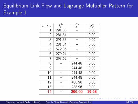
Equilibrium Link Flow and Lagrange Multiplier Pattern forExample 1
Link a f 1∗a f 2∗a λ∗a1 291.33 – 0.002 281.54 – 0.003 291.33 – 0.004 281.54 – 0.005 572.86 – 0.006 279.24 – 0.007 293.62 – 0.008 – 244.48 0.009 – 244.48 0.00
10 – 244.48 0.0011 – 244.48 0.0012 – 488.96 0.0013 – 288.96 0.0014 – 200.00 19.68
Nagurney, Yu and Besik (UMass) Supply Chain Network Capacity Competition NEDSI
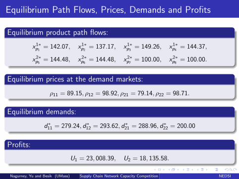
Equilibrium Path Flows, Prices, Demands and Profits
Equilibrium product path flows:
x1∗p1 = 142.07, x1∗p2 = 137.17, x1∗p3 = 149.26, x1∗p4 = 144.37,
x2∗p5 = 144.48, x2∗p6 = 144.48, x2∗p7 = 100.00, x2∗p8 = 100.00.
Equilibrium prices at the demand markets:
ρ11 = 89.15, ρ12 = 98.92, ρ21 = 79.14, ρ22 = 98.71.
Equilibrium demands:
d∗11 = 279.24, d∗12 = 293.62, d∗21 = 288.96, d∗22 = 200.00
Profits:
U1 = 23, 008.39, U2 = 18, 135.58.
Nagurney, Yu and Besik (UMass) Supply Chain Network Capacity Competition NEDSI

Example 2: An External Distribution Center is MadeAvailable But Only Farmer 2 Is Considering It
External distribution center has become available but only the secondfarmer is interested in considering it.
k kk k kk k kk k k kk kFarm 1 Farm 2
Production
1 2
M11 M1
2 M21 M2
2
Transportation
D11,1 OD1,1 D2
1,1
D11,2 OD1,2 D2
1,2
Storage
R1 R2
Distribution
1 8 9
10 11
2
3 4
5
6 7 13 14
1219
20 21
17 18
HHHH
HHHj
XXXXXXXXXXXXXXz
��
��
@@@@R
����
����
��������������9
? ? ?
@@@@R
��
��
@@@@R
�����
���
��
��
��������������9
@@@@R
��
��
@@@@R
��
��
Nagurney, Yu and Besik (UMass) Supply Chain Network Capacity Competition NEDSI
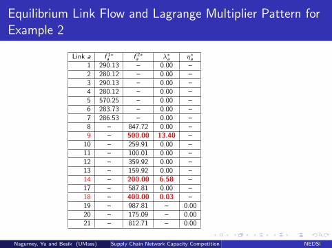
Equilibrium Link Flow and Lagrange Multiplier Pattern forExample 2
Link a f 1∗a f 2∗a λ∗a η∗a1 290.13 – 0.00 –2 280.12 – 0.00 –3 290.13 – 0.00 –4 280.12 – 0.00 –5 570.25 – 0.00 –6 283.73 – 0.00 –7 286.53 – 0.00 –8 – 847.72 0.00 –9 – 500.00 13.40 –
10 – 259.91 0.00 –11 – 100.01 0.00 –12 – 359.92 0.00 –13 – 159.92 0.00 –14 – 200.00 6.58 –17 – 587.81 0.00 –18 – 400.00 0.03 –19 – 987.81 – 0.0020 – 175.09 – 0.0021 – 812.71 – 0.00
Nagurney, Yu and Besik (UMass) Supply Chain Network Capacity Competition NEDSI
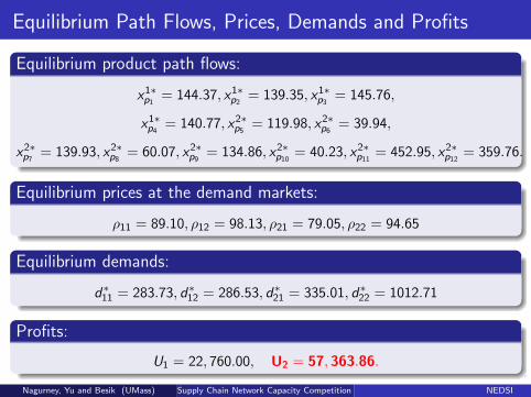
Equilibrium Path Flows, Prices, Demands and Profits
Equilibrium product path flows:
x1∗p1 = 144.37, x1∗p2 = 139.35, x1∗p3 = 145.76,
x1∗p4 = 140.77, x2∗p5 = 119.98, x2∗p6 = 39.94,
x2∗p7 = 139.93, x2∗p8 = 60.07, x2∗p9 = 134.86, x2∗p10 = 40.23, x2∗p11 = 452.95, x2∗p12 = 359.76.
Equilibrium prices at the demand markets:
ρ11 = 89.10, ρ12 = 98.13, ρ21 = 79.05, ρ22 = 94.65
Equilibrium demands:
d∗11 = 283.73, d∗12 = 286.53, d∗21 = 335.01, d∗22 = 1012.71
Profits:
U1 = 22, 760.00, U2 = 57, 363.86.
Nagurney, Yu and Besik (UMass) Supply Chain Network Capacity Competition NEDSI
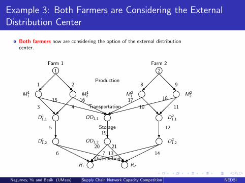
Example 3: Both Farmers are Considering the ExternalDistribution Center
Both farmers now are considering the option of the external distributioncenter.
k kk k kk k kk k k kk kFarm 1 Farm 2
Production
1 2
M11 M1
2 M21 M2
2
Transportation
D11,1 OD1,1 D2
1,1
D11,2 OD1,2 D2
1,2
Storage
R1 R2
Distribution
1 8 9
10 11
2
3 4
5
6 7 13 14
1219
20 21
171615 18
HHHH
HHHj
XXXXXXXXXXXXXXz
��
��
@@@@R
����
����
��������������9
? ? ?
@@@@R
XXXXXXXXXXXXXXz
��
��
HHHHH
HHj
@@@@R
�����
���
��
��
��������������9
@@@@R
����
@@@@R
��
��
Nagurney, Yu and Besik (UMass) Supply Chain Network Capacity Competition NEDSI

Equilibrium Link Flow and Lagrange Multiplier Pattern forExample 3
Link a f 1∗a f 2∗a λ∗a η∗a1 596.67 – 0.00 –2 708.78 – 0.00 –3 142.33 – 0.00 –4 245.04 – 0.00 –5 387.37 – 0.00 –6 177.57 – 0.00 –7 209.80 – 0.00 –8 – 778.03 0.00 –9 – 500.00 10.63 –
10 – 247.45 0.0011 – 120.70 0.0012 – 368.15 0.0013 – 168.14 0.0014 – 200.00 10.20 –15 454.34 – 0.00 –16 463.74 – 0.00 –17 – 530.58 0.00 –18 – 379.29 0.00 –19 918.08 909.88 – 0.0020 480.99 346.97 – 0.0021 437.10 562.91 – 12.41
Nagurney, Yu and Besik (UMass) Supply Chain Network Capacity Competition NEDSI
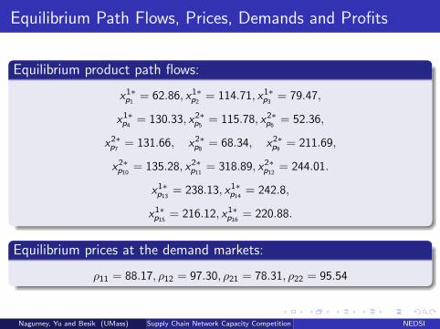
Equilibrium Path Flows, Prices, Demands and Profits
Equilibrium product path flows:
x1∗p1 = 62.86, x1∗p2 = 114.71, x1∗p3 = 79.47,
x1∗p4 = 130.33, x2∗p5 = 115.78, x2∗p6 = 52.36,
x2∗p7 = 131.66, x2∗p8 = 68.34, x2∗p9 = 211.69,
x2∗p10 = 135.28, x2∗p11 = 318.89, x2∗p12 = 244.01.
x1∗p13 = 238.13, x1∗p14 = 242.8,
x1∗p15 = 216.12, x1∗p16 = 220.88.
Equilibrium prices at the demand markets:
ρ11 = 88.17, ρ12 = 97.30, ρ21 = 78.31, ρ22 = 95.54
Nagurney, Yu and Besik (UMass) Supply Chain Network Capacity Competition NEDSI
Equilibrium Demands and Profits
Equilibrium demands:
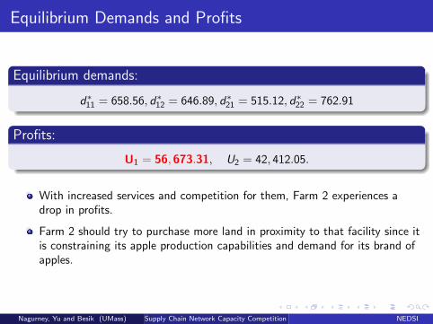
d∗11 = 658.56, d∗12 = 646.89, d∗21 = 515.12, d∗22 = 762.91
Profits:
U1 = 56, 673.31, U2 = 42, 412.05.
With increased services and competition for them, Farm 2 experiences adrop in profits.
Farm 2 should try to purchase more land in proximity to that facility since itis constraining its apple production capabilities and demand for its brand ofapples.
Nagurney, Yu and Besik (UMass) Supply Chain Network Capacity Competition NEDSI

Example 4: A Supply Chain Disruption Has DamagedFarmers’ Distribution Centers
Both farmers have their storage facilities made unavailable due to a naturaldisaster, such as flooding.
Picking has not been affected.
k kkk
k k k kk kFarm 1 Farm 2
Production
Transportation
1 2
M11 M1
2 M21 M2
2
OD1,1
OD1,2
Storage
R1 R2
Distribution
1 8 92
19
20 21
171615 18
����
@@@@R
?
XXXXXXXXXXXXXXz
HHHHH
HHj
�����
���
��������������9
@@@@R
����
@@@@R
��
��
Nagurney, Yu and Besik (UMass) Supply Chain Network Capacity Competition NEDSI

Equilibrium Link Flow and Lagrange Multiplier Pattern forExample 4
Link a From Node To Node f 1∗a f 2∗a λ∗a η∗a1 1 M1
1 513.45 – 0.00 –2 1 M1
2 500.00 – 0.00 –8 2 M2
1 – 574.26 0.00 –9 2 M2
2 – 400.00 0.00 –15 M1
1 OD1,1 513.45 – 0.00 –16 M1
2 OD1,1 500.00 – 3.07 –17 M2
1 OD1,1 – 574.26 0.00 –18 M2
2 OD1,1 – 400.00 9.38 –19 OD1,1 OD1,2 1013.45 974.26 – 0.0020 OD1,2 R1 576.09 411.62 – 0.0021 OD1,2 R2 437.36 562.64 – 15.75
Nagurney, Yu and Besik (UMass) Supply Chain Network Capacity Competition NEDSI

Equilibrium Path Flows, Prices, Demands and Profits
Equilibrium product path flows:
x1∗p13 = 291.20, x1∗p14 = 284.90, x1∗p15 = 225.25,
x1∗p15 = 222.25, x1∗p16 = 215.10,
x2∗p9 = 249.52, x2∗p10 = 162.10, x2∗p11 = 324.75, x2∗p12 = 237.90.
Equilibrium prices at the demand markets:
ρ11 = 88.44, ρ12 = 98.13, ρ21 = 78.60, ρ22 = 96.75.
Equilibrium demands:
d∗11 = 576.09, d∗12 = 437.36, d∗21 = 411.62, d∗22 = 562.64.
Profits:
U1 = 46, 427.75, U2 = 29, 237.16.
Nagurney, Yu and Besik (UMass) Supply Chain Network Capacity Competition NEDSI

Summary of the Profits in Different Examples
Example Farm 1 Profit Farm 2 Profit1 23,008.39 18,135.582 22,760.00 57,363.863 56,673.31 42,412.054 46,427.75 29,237.16
Both farms benefit by utilizing the external distribution centers as revealedby the profit increase from Example 1 to Example 3.
Using an external distribution center increases the farm profits, as it is inExample 2.
Nagurney, Yu and Besik (UMass) Supply Chain Network Capacity Competition NEDSI

Conclusions
We developed a supply chain network framework using game theory inwhich multiple manufacturers/producers have their own production facilities,distribution centers and freight services.
We focused on capacity competition and considered outsourcing throughthe product storage to external distribution centers who also provide freightservice provision to the demand points.
Due to the shared constraints, we utilize the concept of variationalequilibrium, which is a special case of a Generalized Nash Equilibrium.
We then illustrate the novel supply chain game theory framework with acase study consisting of producers that are apple farmers.
Nagurney, Yu and Besik (UMass) Supply Chain Network Capacity Competition NEDSI

THANK YOU!
For more information: https://supernet.isenberg.umass.edu/
Nagurney, Yu and Besik (UMass) Supply Chain Network Capacity Competition NEDSI