S1

Supporting Information

Towards an atomistic understanding of electrocatalytic partial

hydrocarbon oxidation: propene on palladium

Anna Winiwartera∥, Luca Silviolib∥, Soren B. Scotta, Kasper Enemark-Rasmussenc, Manuel Sariҫb,

Daniel B. Trimarcod, Peter C. K. Vesborga, Poul G. Mosese, Ifan E. L. Stephensf, Brian J. Segera,

Jan Rossmeislb*, Ib Chorkendorffa*

aSection for Surface Physics and Catalysis, Department of Physics, Technical University of Denmark, DK-2800 Kgs.

Lyngby, Denmark

bNano-Science Center, Department of Chemistry, University of Copenhagen, Universitetsparken 5, DK-2100

Copenhagen, Denmark

cDepartment of Chemistry, Technical University of Denmark, DK-2800 Kgs. Lyngby, Denmark

dSpectro Inlets, Kgs. Lyngby, DK-2800, Denmark

eHaldor Topsoe A/S, Haldor Topsøes Allé 1, Kgs. Lyngby, DK-2800, Denmark

fDepartment of Materials, Imperial College London, Royal School of Mines, London, SW7 2AZ, UK

Electronic Supplementary Material (ESI) for Energy & Environmental Science.This journal is © The Royal Society of Chemistry 2019

S2

Contents

Experimental details for electrochemical experiments ................................................................................ 3

Electrode characterisation ............................................................................................................................ 5

SEM ........................................................................................................................................................... 5

XPS ................................................................................................................................................................ 6

Determination of ESCA ............................................................................................................................. 8

Additional electrochemical data ................................................................................................................. 10

Chronoamperometry .............................................................................................................................. 10

Additional analysis and discussion of surface oxide formation and Pd dissolution ............................... 12

EC-MS calibration and additional data ....................................................................................................... 17

Product quantification –calibration and validation .................................................................................... 25

Product degradation ................................................................................................................................... 31

NMR analysis of acrolein degradation product ...................................................................................... 31

Additional product analysis data at various conditions .............................................................................. 38

ICP-MS ......................................................................................................................................................... 39

Calculation of reversible potentials ............................................................................................................ 40

Computational details ................................................................................................................................. 42

Propene adsorption mechanism on Pd fcc111 ....................................................................................... 43

Propene degradation on Pd fcc111 ........................................................................................................ 44

Reaction energetics on Pd fcc111, at 0.0 V vs. RHE ................................................................................ 45

References .................................................................................................................................................. 46

S3

Experimental details for electrochemical experiments

The majority of electrochemical bulk experiments was carried out in a conventional 3-compartment

electrochemical glass cell, connected to a gas supply and GC, as described previously1, and shown in

Figure 2 (main text). A Hg/HgSO4 electrode was used as reference, calibrated regularly (at least every

time a new batch of electrolyte was prepared) by measuring the open circuit voltage of a Pt wire

electrode in H2 saturated electrolyte until stable for at least 10 min. Pt mesh was used as counter

electrode. For each experiment, the electrolyte was purged with Ar (5.0, AGA) for at least 15 min in a

beaker, after which it was transferred into the H-cell. The electrolyte volume in the working electrode

compartment was 13 mL. After assembling the cell, the electrolyte in the working compartment was

purged with Ar for another 15 min, keeping the electrode in the headspace. The electrode was

immersed and polarized to 0.471 V vs RHE (potentiostat model SP 150, Bio-Logic), while switching the

gas to propene (4.0, BOC) and purging. After 10 min the gas system was set too loop mode, followed by

injection into the GC and stepping the potential to the final chronoamperometry (CA) potential. After 1h

at constant potential, a gas sample was injected into the GC, followed by purging the electrolyte with Ar

for 10 min to minimize homogeneous reactions with propene thereafter. The electrolyte was analyzed

for liquid products with different methods as soon as possible (see below). In between, samples were

stored in the fridge at 5 °C. Manual ohmic drop compensation (85 %) was employed during CA using the

built-in function in the software EC-Lab. The ohmic drop was determined by electrochemical impedance

spectroscopy of an equivalent electrode in the same setup and assumed to be the same for all

electrodes (25 Ω). The impedance measurements were performed at 0.321 V vs RHE, measuring from

100 kHz to 5 Hz with 10 mV perturbation. The ohmic resistance was determined by fitting with a

R1+R2Q circuit; where take R1 was taken as the ohmic drop for ohmic drop compensation.

S4

Additional experiments were carried out in a conventional RDE setup. Here, the electrolyte was

thoroughly purged with Ar in the cell before immersing the electrode. The ohmic resistance was

determined as described above, and 85 % ohmic drop compensation employed.

S5

Electrode characterisation

SEM

Scanning electron microscope images were obtained using a FEI Quanta FEG 200 ESEM with field

emission gun. SE images were recorded in high vacuum mode, with 15 kV acceleration voltage.

a) b)

Figure S1 SEM images of a high surface area electrode a) as prepared and b) the same electrode after

electrochemical measurements (CVs and 1h CA at ca.1.12V vs RHE). The surface exhibits dendrite-like

crystals with features of nm scale. These structures are still present after electrochemistry.

S6

XPS

X-ray photoelectron spectroscopy was performed on a ThermoScientific Thetaprobe instrument

equipped with an Al Kα x-ray source. The chamber pressure was approx. 1x10-7 mbar, an Ar flood gun

was used for charge neutralisation of the samples. For survey spectra 20 scans were recorded with

50 ms dwell time per 1 eV step. For element detail scans 50 scans were recorded in 0.1 eV steps with

200 ms dwell time.

a)

S7

b)

c)

Figure S2 XPS spectra of a high surface are Pd electrodes as prepared (black) and after electrochemistry

(1 h CA at 1.09 V vs RHE, red) a) survey spectrum, b) carbon 1s peak, c) palladium 3d peak

S8

Determination of ESCA

The electrochemical surface area of each electrode was determined after the respective electrochemical

test from the oxide reduction peak in CVs (50 mV/s between 0.32 and 1.4 V vs RHE) in 0.1 M HClO4.

Before recording CVs, the electrode was transferred to a separate 3-compartment cell, to avoid

influencing the product distribution. To calculate the area of the oxide reduction peak, the cathodic scan

was integrated between 0.4 and 0.9 V vs RHE. The capacitive contribution was determined from the

average current between 0.37 and 0.46 V vs RHE and subtracted, as described in 18. The surface area of

four freshly prepared electrodes was determined by CO stripping, using a charge per area of

410 µC/cm2. This is based on the assumption of adsorption of one CO molecule per surface atom (i.e. 2

e- per atom) on a surface consisting of equal amounts of (111), (110) and (100) facets, as given in 2. On

the same electrodes, the oxide reduction charge was measured as described. The correlation between

ESCA from CO stripping and oxide reduction charge was used to estimate the ESCA for the electrodes

used in this study. An example of a CO stripping CV is given in Figure S3a. We did not use CO stripping

directly, to avoid contamination of the setup with CO, minimizing the risk of introducing additional

errors to the product distribution.

As CV data was not available for all electrodes, the ESCA for the missing electrodes was estimated based

on the propene adsorption charge: A correlation between propene adsorption charge (measured while

purging the cell with propene at constant potential), and the ESCA was established using data from the

other electrodes (see Figure S3). This estimation was used for electrodes used for propene oxidation at

potentials 0.7, 0.85, 1.0, 1.1 and 1.2 V (one for each potential, respectively).

S9

Figure S3 a) CO stripping CVs at recorded at 20 mV/s: For determination of the CO oxidation charge, the

peak at 0.9 V was integrated (shaded in red) and Pd oxidation background subtracted (shaded grey

area). The PdO reduction charge was determined from the shaded yellow area. For calibration additional

CVs recorded at 50 mV/s (not shown) were used. b) Propene adsorption charge during initial purging

with propene at constant potential (0.471 V vs RHE) as a function of ESCA as determined from

integration of the oxide reduction peaks (blue dots, left y-axis). The same data normalized to ECSA is

shown on the right y-axis (red crosses).

S10

Additional electrochemical data

Chronoamperometry

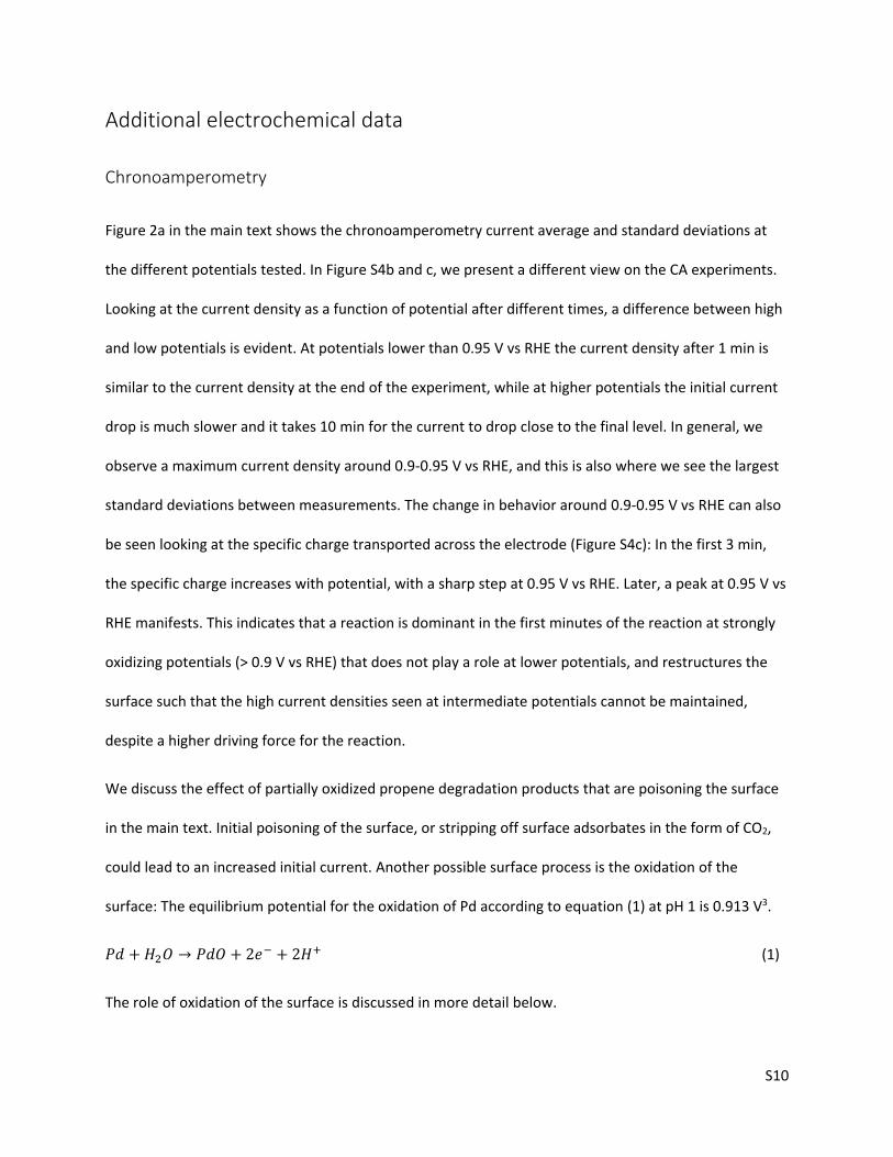
Figure 2a in the main text shows the chronoamperometry current average and standard deviations at

the different potentials tested. In Figure S4b and c, we present a different view on the CA experiments.

Looking at the current density as a function of potential after different times, a difference between high

and low potentials is evident. At potentials lower than 0.95 V vs RHE the current density after 1 min is

similar to the current density at the end of the experiment, while at higher potentials the initial current

drop is much slower and it takes 10 min for the current to drop close to the final level. In general, we

observe a maximum current density around 0.9-0.95 V vs RHE, and this is also where we see the largest

standard deviations between measurements. The change in behavior around 0.9-0.95 V vs RHE can also

be seen looking at the specific charge transported across the electrode (Figure S4c): In the first 3 min,

the specific charge increases with potential, with a sharp step at 0.95 V vs RHE. Later, a peak at 0.95 V vs

RHE manifests. This indicates that a reaction is dominant in the first minutes of the reaction at strongly

oxidizing potentials (> 0.9 V vs RHE) that does not play a role at lower potentials, and restructures the

surface such that the high current densities seen at intermediate potentials cannot be maintained,

despite a higher driving force for the reaction.

We discuss the effect of partially oxidized propene degradation products that are poisoning the surface

in the main text. Initial poisoning of the surface, or stripping off surface adsorbates in the form of CO2,

could lead to an increased initial current. Another possible surface process is the oxidation of the

surface: The equilibrium potential for the oxidation of Pd according to equation (1) at pH 1 is 0.913 V3.

𝑃𝑑 + 𝐻2𝑂 → 𝑃𝑑𝑂 + 2𝑒− + 2𝐻+ (1)

The role of oxidation of the surface is discussed in more detail below.

S11

a

b c

Figure S4 a) Average and standard deviation for CAs at each 3 different potentials: 0.85, 0.90 and 0.95 V

vs RHE) in propene, based on three individual measurements each. The vertical lines indicate where the

values for current density and charge density shown in b were taken from. b) Current density and charge

density passed after certain amounts of time extracted from CAs.

S12

Additional analysis and discussion of surface oxide formation and Pd dissolution

The dissolution of Pd (equation (2)) depends on the Pd concentration in solution according to equation

(3), with R being the gas constant, T the absolute temperature, and F Faraday’s constant.

Pd → Pd2+ + 2e− (2)

𝑈0 = 0.987 +𝑅𝑇

2𝐹𝑙𝑜𝑔 [Pd2+] (3)

Catalyst dissolution was observed at all potentials, peaking at 0.95 V vs RHE. Pourbaix diagrams 3 show

that Pd dissolution to Pd2+ starts around 0.8 V vs. RHE. Detailed studies on Pd dissolution studies report

an onset of dissolution in potentiodynamic conditions at 0.85 V vs RHE.4 The highest dissolution was

observed at 0.95 V vs RHE. We hypothesize that restructuring of the surface close to the oxidation

potential facilitates dissolution, while the oxide layer likely present at higher potentials (see below) acts

as a passivation layer, reducing further corrosion. Actual Pd dissolution is expected to be higher than the

values presented in this work, as substantial amounts of Pd ions react homogeneously with propene

(see below) and are then are obscured when determining the concentration with ICP-MS. As the

homogenous reaction yields acetone, the charge involved in this dissolution is, however, accounted for

in the faradaic efficiency analysis. Dissolution alone is not sufficient to explain the low total faradaic

efficiency. As the current densities are very small, we estimated the possible charge contribution of the

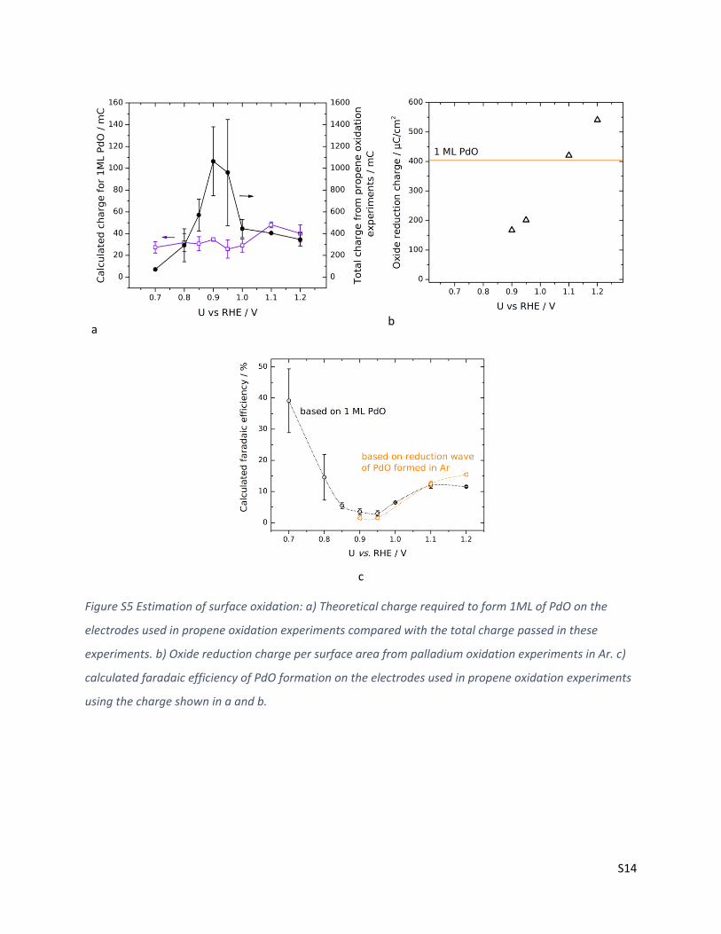
formation of one monolayer (ML) PdO on the electrode surface. Assuming an atom density of 1.26·1015

atoms/cm2 (the average over low index facets) we calculated the faradaic efficiency for the formation of

a monolayer of PdO for the propene oxidation experiments shown before: First the charge required for

oxidation of one unit surface area was calculated. This specific charge was then multiplied with the

surface area of the respective electrodes of the individual propene oxidation experiments at different

potentials (shown in Figure S5a). From this the faradaic efficiency was determined for the individual

experiments (shown in Figure S5c). The assumption for surface atom density is justified as we used the

S13

same atom density when determining the surface area. However, in that case we use this atom density

to convert the CO oxidation charge from a CO stripping experiment to a surface area, under the

assumption of having one CO molecule per Pd surface atom (see section on CO stripping).

The theoretical value for PdO faradaic efficiency is compared to the faradaic efficiency obtained from

separate experiments in Ar under similar conditions as for propene oxidation. Here we determined the

charge for surface oxide formation by integrating the oxide reduction wave in an anodic potential sweep

following the oxidation sequence. Here the oxide reduction charge was normalized to the surface area

of the electrodes (shown in Figure S5b), and as for the theoretical calculation, multiplied with the

surface area of the electrodes used in the propene oxidation experiments to estimate a faradaic

efficiency. Both methods lead to similar estimates and allow the assumption that surface oxidation

accounts for 10-15 % of the total charge at strongly oxidizing potentials. At potentials below 0.85 V vs

RHE, the theoretical value is expected to overestimate the actual contribution, as surface oxidation is

inhibited by adsorbates at these potentials (see Figure 2 in the main text).

S14

a b

c

Figure S5 Estimation of surface oxidation: a) Theoretical charge required to form 1ML of PdO on the

electrodes used in propene oxidation experiments compared with the total charge passed in these

experiments. b) Oxide reduction charge per surface area from palladium oxidation experiments in Ar. c)

calculated faradaic efficiency of PdO formation on the electrodes used in propene oxidation experiments

using the charge shown in a and b.

S15

Figure S6 Allyl alcohol oxidation: 0.1 M HClO4 with 0.1 mM allyl alcohol at 0.8 and 0.9 V vs RHE (blue and

grey line, respectively). Propene oxidation current at 0.9 V vs RHE (grey) added for comparison. Product

distribution at 0.8 V vs RHE reported in Figure 8 in the main text.

S16

Figure S7 Allyl alcohol oxidation: 0.1 M HClO4 with 10 mM allyl alcohol at 0.8, 0.9, and 1.1 V vs RHE

(green and grey, orange, and blue line, respectively). Propene oxidation current at 0.9 V vs RHE (red)

added for comparison. Product distribution for the experiment at 0.8 V vs RHEreported in Figure 8 in the

main text.

S17

EC-MS calibration and additional data

The in-operando mass spectrometry setup (electrochemistry-mass spectrometry, EC-MS) described in 5

is based on a membrane microchip interfacing the electrochemical environment with the a vacuum

system without differential pumping. Gaseous products evaporate through the micro-perforated

membrane of the microchip and are delivered to the mass spectrometer through a capillary in the

microchip without differential pumping. The gas saturating the electrolyte (He, CO, or propene) is

simultaneously introduced through the microchip membrane. The working distance between the

working electrode and the membrane was 100 μm. The electrolyte was stagnant for all experiments to

maximize sensitivity and to have well-defined mass transport between the membrane and the

electrode.

Masses m/z=2 (H2), m/z=4 (He), m/z=18 (H2O), m/z=28 (CO, N2), m/z=29 (propane), m/z=32 (O2), m/z=41

(propene), and m/z=44 (CO2) were monitored during experiments. Mass spectra were taken while

holding the electrode at various potentials in propene-saturated electrolyte, and all fragments could be

attributed to these species. This setup is unfortunately not sensitive to products with low vapor

pressure, i.e., products that are liquid at room temperature. Propene, propane, and CO2 were quantified

using their mass fragment of highest intensity: m/z=41 for propene, m/z=29 for propane, and m/z=44

for CO2, calibrated in-situ as follows: CO stripping experiments at the start and end of each experimental

run were used to calibrate the CO2 signal, as the amount of CO2 produced can be determined from the

electrochemical data. To calibrate the propene and propane signals, we measured propene reduction to

propane by flowing propene through the chip and performing two-minute pulses of constant cathodic

current. No hydrogen was observed when the cathodic current did not exceed -400 µA, and so the

amount of propane produced could be calculate by dividing the charge passed by -2F. Propene was

calibrated by assuming ideality of the propene/propane gas mixture, i.e., that the amount of propene

S18

displaced from the carrier gas was equal to the amount of propane produced. As propane also has mass

fragments at m/z=44 and m/z=41, the mass signal at m/z=29 multiplied by the appropriate factor was

subtracted from these signals before calculating the CO2 and propene fluxes, respectively. All of these

calibration experiments are shown in Figure S8.

S19

Figure S8 EC-MS calibration of propene and propane. a) 70 eV electron-impact ionization mass spectra

for propene (C3H6) and propane (C3H8) normalized to the most intense peak, 41 for propene and 29 for

propane. From NIST. b) Calibration experiment, as an EC-MS plot. The signals at m/z=2 (H2), m/z=29, and

m/z=41 are shown. The potential is cycled between a resting potential of 0.7 V vs RHE and a cathodic

working potential which is stepped down. c) The integrated MS signals (left y-axis) and electrochemical

charge passed (ΔQ, right y-axis) as a function of working potential. The m/z=41 signal (red diamonds)

includes contributions from both propene and propane. The contribution from propane is calculated by

multiplying the m/z=29 signal by the ratio of m/z=41 and m/z=29 intensity in the NIST spectrum for

propane, and subtracted (red circles). d) The absolute difference of the integrated MS signals from the

background values plotted against ΔQ/(2F), which is the amount of propene converted to propane

assuming no other processes. The rightmost point, taken at -0.1 V vs RHE, is excluded from the line of

best fit, since H2 is produced. The slope of the lines of best fit for the m/z=29 and the corrected m/z=41

signals are the calibration factors for propane at m/z=29 and propene at m/z=41, respectively.

S20

CO-stripping

As an illustration of this technique, a CO stripping experiment performed on a palladium foam electrode

is shown in Figure S9a. In this plot, electrochemical data (potential and current) and mass spectrometric

data (calibrated signals for the primary mass fragments of select gases) are plotted together on a common

time axis. After dosing and purging CO, the electrode is scanned to a cathodic potential of 0.05 V vs RHE,

where Pd would normally show a strong hydrogen absorption current, and the lack of current on the first

scan is evidence that the surface is saturated with CO. On the subsequent anodic scan, CO is stripped off

with an oxidative current and a CO2 signal is observed. After this, hydrogen absorption and evolution are

observed in the current and mass spectrometer signals at ~300 s. The oscillations of the current are due

to the high impedance in the thin layer of electrolyte.

In addition to providing a demonstration of the technique with a familiar experiment, the CO stripping

results are also used to characterize the electrode, as also done in the bulk oxidation experiments. The

amount of CO adsorbed is calculated based on the difference of the two CV’s, as shown in Figure S9b,

and the assumption of two electrons per CO molecule. This was found, over CO stripping experiments

on separately prepared electrodes, to be proportional to the palladium reduction wave at ~0.8 V vs RHE,

indicating that both can be used to describe the electrochemical surface area, as also established in the

literature.2,6

S21

Figure S9 CO stripping calibration. a, EC-MS plot of a CO stripping experiment. CO is dosed at 0.3 V vs

RHE and purged. Then, the potential is scanned cathodically at 10 mV/s to 0.05 V vs RHE and then cycled

between 0.05 V and 1.45 V vs RHE while the desorption products are monitored. The oscillations at

~620 s are due to the large hydrogen absorption/evolution current on the CO-free surface and the high

impedance of the setup. The electrochemistry data from the stripping cycle (cycle 1) and subsequent

cycle (cycle 2) are replotted in b. The integration used for determining the CO monolayer amount and the

palladium reduction charge are indicated.

S22

Figure S10 Propene stripping data.Propene stripping raw data plotted vs time (a, c, e) , and calibrated data from the

stripping cycles plotted vs potential (b, d, f). The propene dosing potential were 0.4 V vs RHE (a, b), 0.65 V vs RHE (c, d), and 0.9

V vs RHE (e, f). All of the time axes refer to the same t=0. The value of MLCO, is based on the Pd reduction as indicated. The

oxidation wave at ~0.9 V vs RHE in the second cycle of f is attributed to further oxidation of liquid products formed during the

propene dose.

S23

Figure S10 shows the propene stripping experiments from main text Figure 6 in more detail. After each

propene strip the electrode is cycled several times to ensure a clean surface for the next propene dose,

but a majority of desorption products comes off during this first cycle. When plotted as a cyclic

voltammogram Figure S10b, d & f, a clear stripping peak is visible at all dosing potentials. When propene

is dosed at a potential at which significant amounts of liquid products are formed in the

chronoamperometry experiments (main text Figure 4), there is also a notable oxidation peak in the

second cycle (Figure S10f), with an earlier (more cathodic) onset than the stripping peak in the first

cycle. We attribute this peak in the second cycle to further oxidation of the liquid products produced

while dosing propene, which cannot be oxidized during the first cycle because the surface is poisoned.

Further oxidation of liquid products may also contribute to the CO2 detected during the cathodic sweep.

However, cathodic-sweep CO2 is also observed for dosing potentials at which liquid products are not

formed, and so this cannot fully explain the feature, which we will not comment on further in this work.

Figure S11 Normalized propene stripping results. Integrated amounts of propene stripping products

normalized to the theoretical monolayer CO calculated based on the charge passed during the Pd

reduction wave

S24

Figure S12 Propene adsorption transients. a, Current vs time during introduction of propene at various

electrode potentials. t=0 is the time at which propene was dosed, based on the mass spectrometer

signal. The steady-state oxidation current is indicated b, Integrated propene adsorption transient,

defined as the initial current in excess of the steady-state current, co-plotted with the steady-state

current. Both are normalized to MLCO. Since the current when propene is dosed is a complex convolution

of adsorption and oxidation, not much information can be drawn from the adsorption transients.

S25

Product quantification –calibration and validation

Calibration standards for product quantification were prepared by dilution of the pure compounds with

0.1 M HClO4. Acrolein was first dissolved in 1 mL acetone to prevent polymerization on contact with

water. Mixed standards containing at least three different compounds were used in all cases. Calibration

lines were calculated by linear least square fitting of at least 5 different concentrations. The regression

was first calculated without constraints. If the calculated y-intercept was smaller than the standard error

(SEy), the regression was recalculated with a forced y-intercept of 0.

GC

An Agilent 7890A instrument was used for both gas chromatography (GC), and static headspaces gas

chromatography (HS-GC) measurements. The gas from the sample loop connected to the headspace of

the electrochemical cell was injected into a HP-PLOT Q column (45m length, 0.53 mm diameter, 40.0 µm

film thickness; flame ionization detector) and a Molsieve column (30m length, 0.53 mm diameter,

25.0 µm film thickness; thermal conductivity detector) in a ratio 0.5:1 (inlet temperature 150 °C). The

temperature program for gas analysis was hold 6 min at 35 °C, ramp with 10 °C/min to 60 °C, hold at

60 °C for 8 min, followed by a post run at 230 °C for 10 min. The signal in the FID detector was used for

the quantification of CO2. Calibration was done by oxidation of CO on Pt foil and comparison of the

charge with the signal intensity.

HS-GC

The GC was coupled to an Agilent 7694E headspace sampler. 10 mL glass vials were filled with 5 mL

electrolyte and sealed. Gas was taken from the headspace after equilibration at 70 °C for 15 min. Loop

and transfer line were kept at 110 °C and 120 °C, respectively. Injection into a HP-PLOT Q column (45m

length, 0.53 mm diameter, 40.0 µm film thickness; flame ionization detector) followed in a 0.5:1 ratio at

S26

150 °C. The temperature program was hold 33 min at 120 °C, ramp with 10 °C/min to 230°C, hold at

230°C for 10 min, followed by a post run at 230 °C for 10 min.

Duplicate measurements were attempted, but the fast degradation of the products at elevated

temperatures in the autosampler lead to erroneous values.

HS-GC shows peaks for acetone, propanal, acrolein and isopropanol. We only used the method for the

quantification of acetone and propanal as other methods proved to be more reliable/sensitive for the

other compounds.

Given value

Average Rel. STD

(precision)

Rel deviation (accuracy)

µmol / L µmol / L % %

10 8.79 7.45 -12.06

50 47.89 1.72 -4.22

100 89.39 10.14 -10.61

250 239.53 2.12 -4.19

Figure S13 Acetone calibration: Calibration line and statistical parameters (left) and details of the

validation analysis (right). For the calibration, standards of 5 concentrations were prepared. Three

individual samples of each standard were measured. For validation, standards of 4 different

concentrations were prepared separately and again 3 individual samples each were measured. The rel.

standard deviation between these 3 samples is given as an estimate for the precision of the method. The

relative deviation of the average value from the given value can serve as estimate for the accuracy

S27

Given value Average Rel. STD

(precision)

Rel deviation (accuracy)

µmol / L µmol / L % %

10 9.08 10.76 -9.24

50 62.05 4.77 24.10

10 7.88 23.52 -21.20

50 50.70 6.12 1.40

Figure S14 Propanal calibration. See Figure S13 for details. Here validation was based on only two

concentrations, but each prepared twice.

HPLC

An Agilent 1200 series high performance liquid chromatograph was used, equipped with with

autosampler, degasser, quarternary pump, and diode array detectors (UV-VIS range). A BIORAD, Aminex

HPX-87H column was employed, heated externally to 50 °C. 5mM H2SO4 (diluted from concentrated

H2SO4, suprapur, Merck with ultrapure water) was used as eluent with a flow rate of 0.6mL/min. The

injection volume was 30µL.

HPLC was used for only for acrolein and acrylic acid due to the need for sufficient absorption in the

available UV-VIS range.

S28

Given value

Average Rel. STD

(precision) Rel deviation

(accuracy)

µmol / L µmol / L % %

5 5.91 7.19 18.22

50 56.58 4.47 13.16

250 275.23 4.53 10.09

Figure S15 Acrolein calibration. See Figure S13 for details. Validation is based on three injections of the

same standard at three different concentrations.

Given value

Average Rel. STD

(precision) Rel deviation

(accuracy)

µmol / L µmol / L % %

5 4.90 2.48 -2.09

10 9.89 1.14 -1.09

50 49.64 0.20 -0.72

100 100.79 1.00 0.79

250 249.04 0.09 -0.38

Figure S16 Acrylic acid calibration. See Figure S13 for details. Validation is based on three injections of

the same standard at five different concentrations.

NMR

The 1H NMR spectra were acquired on a Bruker AVANCEIII HD spectrometer operating at a 1H frequency

of 800.182 MHz and equipped with a 5 mm TCI Cryoprobe (Bruker Biospin). The strong water resonance

was suppressed utilizing a “perfect-echo” excitation sculpting pulse sequence (zgesgppe in the Bruker

pulse sequence library) with a 2000 s selective 180o inversion pulse. A total of 256 transient scans were

S29

acquired for each spectrum with an acquisition time of 3.4 seconds and an interscan delay of 10

seconds. For each FID 64K complex points were acquired and the FID was then zero-filled to 64K real

points before Fourier transformation (FT). An exponential apodization function with lb = 0.3 Hz was

applied to the FID’s prior to FT.

NMR samples were prepared by addition of 100 µL D2O and 25 µL of a 950 µM DMSO in H2O as internal

standard to 475 µL of the liquid sample, resulting in a DMSO concentration corresponding to 50 µM in

the undiluted sample. qNMR was used to quantify isopropanol, allyl alcohol and propylene glycol. For

these compounds, external calibration lines were measured (see Figure S17, Figure S18 and Figure S19).

Given value

Average Rel. STD

(precision) Rel deviation

(accuracy)

µmol / L µmol / L % %

5 3.93 - -21.33

10 8.83 - -11.71

50 49.92 - -0.15

100 101.62 - 1.62

Figure S17 Allyl alcohol calibration: peak at 4.02ppm. See Figure S13 for details. Validation is based on

the measurement of one individually prepared sample for each concentration.

S30

Given value

Average Rel. STD

(precision) Rel deviation

(accuracy)

µmol / L µmol / L % %

5 6.20 - 24.04

10 11.18 3.35 11.76

50 47.47 2.75 -5.05

100 96.43 1.85 -3.57

250 239.15 3.25 -4.34

Figure S18 Isopropanol calibration: peak at 1.07 ppm. See Figure S13 for details. Validation is based on

the measurement of two individual samples with 10 µM analyte and four individual samples at three

higher concentrations.

Given value

Average Rel. STD

(precision) Rel deviation

(accuracy)

µmol / L µmol / L % %

5 6.05 - 20.93

10 11.23 5.18 12.26

50 50.63 7.07 1.26

100 106.77 5.04 6.77

250 264.38 6.29 5.75

Figure S19 Propylene glycol calibration: peak at 3.35 ppm. See Figure S13 for details. Validation is based

on the measurement of two individual samples with 10 µM analyte and four individual samples at three

higher concentrations.

S31

Product degradation

The change in acrolein and acrylic acid concentration was monitored over at least 5 h for all samples

using HPLC. Within the first 40 min, we observed no changes in acrolein and acrylic acid concentration

exceeding the measurement uncertainty, but at longer times an additional peaks started to grow with

concomitant decrease in acrolein concentration. Thus measurements must be done immediately. NMR

was used to monitor long-term stability of all products. Also here additional peaks and loss of acrolein

were observed, while the concentrations of the other products were stable within the measurement

inaccuracy over the first few hours, after which they decreased. In-depth NMR analysis of the additional

growing peaks showed that they can be assigned to two acrolein hydration products in equilibrium with

each other by keto-enol tautomerism: 3-hydroxypropanal and propane-1,3,3-triol (see below for

detailed analysis).

NMR analysis of acrolein degradation product

Six unidentified peaks are observed for acrolein-containing samples in the 1H NMR spectra. The

observed 1H chemical shifts and multiplet splitting of the peaks does not fit with the common

dimerization product of acrolein. Thus, 2D correlation experiments were acquired on a concentrated

sample in an effort to identify the origin of the peaks. The edited HSQC experiment allows for

observation of the 13C chemical shift for the directly bonded carbon atom, as well as the number of

attached protons. With this experiment it is found that peak 1 to 4 can be assigned to methylene

groups, while peak 5 is a single CH and 6 is an aldehyde. The high 1H and 13C chemical shifts of 5

suggest the presence of OH groups in the close vicinity. From COSY and TOCSY experiments it is found

that two spin systems are present; 5-1-3 and 2-4-6/6-2-4. Since peak 6 does not show any correlations in

the COSY spectrum it is not possible to unambiguously identify the order. To verify the position of 6 a

NOESY spectrum was acquired. In the spectrum correlation peaks between 5 and 6, 3 and 4, and 1 and 2

S32

are observed. All of these correlation peaks exhibit the same phase as the diagonal peaks which is a

clear indication that chemical exchange is taking place. Taking into account the 1H and 13C chemical

shift of 3, 4 and 5 we propose that the peaks originate from a keto-gem-diol tautomerization reaction

between 3-hydroxypropanal and propane-1,1,3-triol. To further support this claim we acquired a series

of 1H spectra at different temperatures. The tautomerization reaction should still be slow enough to

observe two different compounds, but the equilibrium of the reaction is expected to shift with

temperature. This is clearly evident from the measured 3/4 and 1/2 integral ratios. Peak 5 is partly

suppressed by the inversion pulse and therefore the measured peak area is inaccurate.

Table 1 H integral ratios measured at different temperatures

293 K 298 K 303 K 313 K

H1/H2 2.48 1.81 1.68 1.25

H3/H4 2.36 1.9 1.73 1.25

H5/H6 1.51 1.01 1.01 0.97

The observed multiplet splittings does not correspond perfectly with the 3-hydroxypropanal and

propane-1,1,3-triol structures; namely the absence of peak-splitting for the aldehyde (6) and the diol (5)

peak. However, this can be explained by the tautomerization reaction. Although the conversion is slow

compared to chemical shift evolution (kHz) it is fast compared to J-coupling evolution (Hz). Thus, the

average life-time of the keto and diol-form is too short to allow for well-resolved observation of the

couplings. Instead a broadening of the peaks is observed.

S33

Figure S20 1H NMR spectrum recorded at 800 MHz. Acquisition parameters as detailed in the

experimental part. The unknown peaks are (6) δ1H 9.62 (s, 1H), (5) 5.08 (t, J = 5.4 Hz, 1H), (4) 3.85 (t, J =

5.4 Hz, 1H), (3) 3.61 (t, J = 6.4 Hz, 1H), (2) 2.67 (t, J = 5.4 Hz, 1H), (1) 1.76 (q, J = 6.1 Hz, 1H).

S34

Figure S21 1H-{13C} edited HSQC spectrum recorded at 800 MHz. 2048 x 512 complex data points (50%

NUS) were acquired with 8 transient scans and an interscan delay of 2 seconds. Linear prediction was

applied in the indirect dimension to yield 512 real points and the data matrix was then zero-filled to 2048

x 1024 real points. A 45oshifted squared cosine function was applied in both dimensions prior to FT. The

aldehyde correlation signal was folded in order to increase acquisition time in the indirect dimension.

Notice that the signal is not properly decoupled due to limited bandwidth of the decoupling pulse.

S35

Figure S22 1H-{1H } NOESY spectrum with 400 ms mixing time recorded at 800 MHz. 2048 x 512 complex

data points were acquired with 64 transient scans and an interscan delay of 2 seconds. The data matrix

was zero-filled to 2048 x 1024 real points. A squared cosine function was applied prior to FT. f

S36

Figure S23 1H-{1H } NOESY spectrum with 400 ms mixing time recorded at 800 MHz. 2048 x 512 complex

data points were acquired with 64 transient scans and an interscan delay of 2 seconds. The data matrix

was zero-filled to 2048 x 1024 real points. A squared cosine function was applied prior to FT

S37

HPLC

Acrolein degradation was also studied with HPLC: The changes in concentration in standards containing

different amounts of acrolein and acrylic acid, at room temperature and 4 °C were monitored. The data

is shown in Figure S24. While the concentration of acrylic acid doesn’t change, the acrolein

concentration decreases significantly at room temperature. At the same time a poorly defined peak

evolves on onset of the acrylic acid peak and it’s increases with time. This growing peak is also observed

in all samples from electrochemical measurements containing acrolein.

a) b)

Figure S24 Degradation of acrolein and acrylic acid standard solutions monitored with HPLC.

a)Chromatograms of the fresh standard, after 2 days in the fridge (4 °C), and after 2 days at room

temperature, respectively. The peaks labelled with “artifact” were also present in blank measurements of

the pure solvent. b) Reduction in peak area of the acrolein peak. Negative values and values greater than

100 % are due to measurement inaccuracy.

S38

Additional product analysis data at various conditions

Figure S25 Partial current density and faradaic efficiency for propanal. The product concentration is very

low resulting in large inaccuracies for the quantification.

Figure S26 Product concentrations of propene oxidation in 0.1 M HClO4 containing different

concentrations of PdCl2 without electrode (as shown in Figure XY in the main text, empty symbols, full

lines) compared with the concentrations obtained under the same conditions with glassy carbon

electrode polarized to 0.9 V vs RHE added (half symbols, dotted lines).

S39

ICP-MS

An iCAP-QC ICP-MS instrument from Thermo Fisher Scientific was used for determination of the

concentration of dissolved Pd in the electrolyte at the end of the chronoamperometry experiments. The

samples were diluted in 0.67 % HNO3 (suprapur, Merck) 1:100 or 1:10, to reach a final concentration

between 1 and 10 ppb.

Calibration samples for quantitative analysis were prepared by diluting a 1000 mgmetal/mL Pd standard in

HCl (SCP Science) to four different concentrations were measured every time before analyzing the

samples. The obtained calibration lines were fitted by linear regression (R2=0.999 or higher for all cases).

S40

Calculation of reversible potentials

Table 2 Overview over thermochemical data used for the calculation of reversible potentials. The source

refers to the source for the standard free enthalpy of formation and the standard entropy. All Henry

constant data is taken from reference 11. The free energy of solvation was calculated from the Henry's

law constant according to equation (4) below. The free energy of formation was calculated from the

standard free enthalpy and entropy of reactants and products

Compound ΔfH⊖ (gas phase) / kJ/mol

S (gas phase) / J/K*mol

Henry constant k0

H / mol/kg*bar ΔGsol J/mol ΔfG⊖ /

kJ/mol Source

H2 0 130.68 NIST7

O2 0 205.15 NIST7

C (s) 5.8 NIST7

H2O(l) -285.83 69.95 -237.14 NIST7

CH2CHCHO (acrolein)

-84 281.12 230 -5275.50 -53.82 Smith8

CH2CHCO2H (acrylic acid)

-323.5 307.73 3100 -19293.20 -270.97 NIST7

CH3COCH3 (acetone)

-217.1 295.46 53 -8215.27 -152.53 NIST7

C3H6 (propene) 20.4 227 0.0092 13234.76 74.79 D'Ans Lax9

CH3CHOCH2 (propylene oxide)

-94.7 287.4 14 -4086.72 -27.73 NIST7

CH3CHOHCHOH (propylene glycol)

-429.8 288 76000 -12905.23 -293.46 NIST7

CH2CHCH2OH (allyl alcohol)

-123.6 - 430 -14851.76 -74.6 chemeo10

CH3CH2CHO (propanal)

-189 304 13 -6358.04 -126.98 NIST7

CO2 (g) -393.5 213.8 Not used 8381.86 -394.35 NIST7

S41

Equation (4) denotes the calculation of the solvation free energy from the Henry’s law constant. R is the

gas constant (R = 8.314 J/(K*mol)), T the temperature (T = 298.15 K)

∆𝐺𝑠𝑜𝑙𝑣𝑎𝑡𝑖𝑜𝑛 = 𝑘𝐻0 ∙ 𝑅 ∙T (4)

The reversible potential for a selection of expected products as given in Figure 1 in the main text was

calculated from the data given in Table 2 according to equation 2. z denotes the number of electrons

transferred in the reaction, and F the faraday constant (F = 96485 C/mol) CO2 was determined in the gas

phase, therefore we did not consider the free energy of solvation for this product.

𝑈𝑟𝑒𝑣 =∑ ∆𝑓𝐺⊝

𝑃𝑟𝑜𝑑𝑢𝑐𝑡𝑠 −∑ ∆𝑓𝐺⊝𝑅𝑒𝑎𝑐𝑡𝑎𝑛𝑡𝑠 +∆𝐺𝑠𝑜𝑙𝑣𝑎𝑡𝑖𝑜𝑛

𝑧∙𝐹 (5)

S42

Computational details

All DFT calculations are performed with the Grid-based Projected Augmented Wave (GPAW) program 12,13

and the Atomic Simulation Environment (ASE) package.14 The Kohn-Sham wavefunctions are represented

in real-space uniform grids (finite difference mode); we use the BEEF-vdW exchange and correlation

functional 15, a grid spacing of 0.18 Å and k-point sampling of (2x2x1). The Palladium metal slab is in FCC

crystal structure and is cut along the (111) plane. We use a (4x4) supercell in the calculations for propene

and a (3x3) supercell for the water oxidation intermediates, both with 4 layers where the 2 bottom layers

are fixed in bulk position. All molecule and adsorbate energetics presented in this work are referenced to

the DFT energy of gas phase propene, hydrogen and water. To calculate all reaction species Gibbs free

energy of formation, the entropy and zero point energy corrections are added to the DFT energies.16

Similarly, the reaction transition state (TS) energies calculated with Nudged Elastic Band17 are corrected

for the entropy and zero point energy contributions. For the TS energy levels, we apply the computational

hydrogen electrode scheme18 with the same scaling factor as the respective initial and final states, as the

reactions considered do not involve any charge transfer to/from the system, therefore the

electrochemical potentials remain unchanged throughout the elementary step. Finally, we included a

correction to account for the water-induced stabilization of *OH intermediate, corresponding to 0.3eV

per adsorbate.19

After publication all structures with total energies will be available on Jan Rossmeisl' group homepage

(http://nano.ku.dk/english/research/theoretical-electrocatalysis/katladb/).

S43

Propene adsorption mechanism on Pd fcc111

Figure S27 - Energetics for the possible adsorption mechanisms of propene on a fcc(111) slab surface.

The vinylic and allylic contribution are decoupled in the red bar values.

In figure 27, C1, C2 and C3 refer to adsorption through proton/electron loss at the terminal unsaturated

carbon, central unsaturated carbon and terminal saturated carbon, respectively. Π refers to

chemisorption by coordination of the double bond with a metal site, without proton electron loss; this is

a potential independent step, as no proton/electron couples are exchanged. Applying anodic potential

lowers the oxidative adsorption energetics proportionally to the number of electron exchanged

(hydrogen computational electrode); for this reason, C1 C2 C3 will bind stronger with applied potential

maintaining the same relative energy gap, while Π energy remains unchanged as potential independent.

Furthermore, this figure illustrates the participation of double bond coordination to C3 adsorption. To

isolate the contribution of double bond, we created a slab where a Pd site is surrounded by an inactive

generic metal. Without neighbouring sites able to interact with the unsaturated bond, the adsorption

energy value is due only to C3 adsorption. We found a relative destabilization of ̴1eV for the C3

adsorption.

S44

Propene degradation on Pd fcc111

Figure S28 Computed energetics for the reaction of degradation of propene on a Pd fcc111 surface. There

is indeed a strong driving force to crack the reactant to smaller carbon fractions, even on a relatively

inert closely packed surface. These 1C fractions are then oxidized to CO2 when enough anodic potential is

applied. Calculations fit the results of propene stripping experiments for the significant amount of CO2

recorded by MS.

S45

Reaction energetics on Pd fcc111, at 0.0 V vs. RHE

Figure S29 Reaction pathway energetics at 0 V vs RHE, referenced to gas phase water and propene.

Comparing the adsorption energy of propene and water as *OH, it is clear the greater affinity of carbon

to Palladium than oxygen. We expect propene to interact with the electrode even at no applied potential,

as the energetics in figure refers to a relatively inert facet of the metal. The ΔG between *CH2CHCH2 and

*OH is in agreement with the onset potential observed in experiments (~0.7V).

S46

References

(1) Bertheussen, E.; Hogg, T. V.; Abghoui, Y.; Engstfeld, A. K.; Chorkendorff, I.; Stephens, I. E. L. ACS

Energy Lett. 2018, 3 (3), 634–640.

(2) Mittermeier, T.; Weiß, A.; Gasteiger, H. A.; Hasché, F. J. Electrochem. Soc. 2017, 164 (12), F1081–

F1089.

(3) Pourbaix, M. Atlas of electrochemical equilibria in aqueous solutions; Pergamon Press, 1974.

(4) Pizzutilo, E.; Geiger, S.; Freakley, S. J.; Mingers, A.; Cherevko, S.; Hutchings, G. J.; Mayrhofer, K. J.

J. Electrochim. Acta 2017, 229, 467–477.

(5) Trimarco, D. B.; Scott, S. B.; Thilsted, A. H.; Pan, J. Y.; Pedersen, T.; Hansen, O.; Chorkendorff, I.;

Vesborg, P. C. K. Electrochim. Acta 2018, 268, 520–530.

(6) Grdeń, M.; Łukaszewski, M.; Jerkiewicz, G.; Czerwiński, A. Electrochim. Acta 2008, 53 (26), 7583–

7598.

(7) NIST Chemistry WebBook, NIST Standard Reference Database Number 69; Linstrom, P. J., Mallard,

W. G., Eds.; National Institute of Standards and Technology: Gaithersburg MD, 20899.

(8) Smith, C. W.; Dehnert, J. Acrolein; Dr. Alfred Hüthig Verlag: Heidelberg, 1975.

(9) Ans, J. d’.; Lax, E. . Taschenbuch für Chemiker und Physiker. - 2: Organische Verbindungen;

Synowietz, C., Ed.; Springer Verlag, 1983.

(10) Céondo. Chemical Properties of 2-Propen-1-ol https://www.chemeo.com/cid/32-070-8/2-

Propen-1-ol (accessed Aug 24, 2018).

(11) Sander, R. Atmos. Chem. Phys. 2015, 15 (8), 4399–4981.

(12) Enkovaara, J.; Rostgaard, C.; Mortensen, J. J.; Chen, J.; Dułak, M.; Ferrighi, L.; Gavnholt, J.;

S47

Glinsvad, C.; Haikola, V.; Hansen, H. A.; Kristoffersen, H. H.; Kuisma, M.; Larsen, A. H.; Lehtovaara,

L.; Ljungberg, M.; Lopez-Acevedo, O.; Moses, P. G.; Ojanen, J.; Olsen, T.; Petzold, V.; Romero, N.

A.; Stausholm-Møller, J.; Strange, M.; Tritsaris, G. A.; Vanin, M.; Walter, M.; Hammer, B.;

Häkkinen, H.; Madsen, G. K. H.; Nieminen, R. M.; Nørskov, J. K.; Puska, M.; Rantala, T. T.; Schiøtz,

J.; Thygesen, K. S.; Jacobsen, K. W. J. Phys. Condens. Matter 2010, 22 (25), 253202.

(13) Hjorth Larsen, A.; Jørgen Mortensen, J.; Blomqvist, J.; Castelli, I. E.; Christensen, R.; Dułak, M.;

Friis, J.; Groves, M. N.; Hammer, B.; Hargus, C.; Hermes, E. D.; Jennings, P. C.; Bjerre Jensen, P.;

Kermode, J.; Kitchin, J. R.; Leonhard Kolsbjerg, E.; Kubal, J.; Kaasbjerg, K.; Lysgaard, S.; Bergmann

Maronsson, J.; Maxson, T.; Olsen, T.; Pastewka, L.; Peterson, A.; Rostgaard, C.; Schiøtz, J.; Schütt,

O.; Strange, M.; Thygesen, K. S.; Vegge, T.; Vilhelmsen, L.; Walter, M.; Zeng, Z.; Jacobsen, K. W. J.

Phys. Condens. Matter 2017, 29 (27), 273002.

(14) Bahn, S. R.; Jacobsen, K. W. Comput. Sci. Eng. 2002, 4 (3), 56–66.

(15) Wellendorff, J.; Lundgaard, K. T.; Møgelhøj, A.; Petzold, V.; Landis, D. D.; Nørskov, J. K.; Bligaard,

T.; Jacobsen, K. W. Phys. Rev. B 2012, 85 (23), 235149.

(16) Rossmeisl, J.; Qu, Z.-W.; Zhu, H.; Kroes, G.-J.; Nørskov, J. K. J. Electroanal. Chem. 2007, 607 (1–2),

83–89.

(17) Jónsson, H.; Mills, G.; Jacobsen, K. W. In Classical and Quantum Dynamics in Condensed Phase

Simulations; WORLD SCIENTIFIC, 1998; pp 385–404.

(18) Nørskov, J. K.; Rossmeisl, J.; Logadottir, A.; Lindqvist, L.; Kitchin, J. R.; Bligaard, T.; Jónsson, H. J.

Phys. Chem. B 2004, 108 (46), 17886–17892.

(19) Calle-Vallejo, F.; Martínez, J. I.; Rossmeisl, J. Phys. Chem. Chem. Phys. 2011, 13 (34), 15639.