supporting online material for - alpha.chem.umb.edu

1

1 Energy and Resources Group (ERG). University of California, Berkeley CA 94720, USA. 2 Goldman School of Public Policy. University of California, Berkeley CA 94720, USA. *Corresponding author: [email protected]. Renewable and Appropriate Energy Laboratory, tel: 510-643-2243, http://rael.berkeley.edu

Supporting Online Material for:

Ethanol Can Contribute To Energy and Environmental Goals

Alexander E. Farrell,1* Richard J. Plevin,1 Brian T. Turner,1,2 Andrew D. Jones,1 Michael O’Hare,2 and Daniel M. Kammen1,2

Version 1.1.1

Updated July 13, 2006

Contents

Updates (July 13, 2006) .................................................................................................................. 2 Updates (May 12, 2006) ................................................................................................................. 2 Methods........................................................................................................................................... 2

The ERG Biofuels Analysis Meta-Model (EBAMM)................................................................ 2 Net energy value ......................................................................................................................... 4

Appropriate Metrics................................................................................................................ 6 Agricultural energy ..................................................................................................................... 7 Net Yield..................................................................................................................................... 8 Biorefinery energy ...................................................................................................................... 9 Coproducts .................................................................................................................................. 9 Regarding Our Use of a Constant Coproduct Credit ................................................................ 11 Fossil Fuel Use.......................................................................................................................... 12 Greenhouse Gas Emissions....................................................................................................... 12 Regarding Lime Application Rate ............................................................................................ 14 Other Questions about USDA Data .......................................................................................... 15

Supporting Text ............................................................................................................................ 16 Sensitivity Analysis .................................................................................................................. 18 EBAMM cases .......................................................................................................................... 20 Errors, Omissions, and Inconsistencies .................................................................................... 21

Explanatory notes for Table S2............................................................................................. 22 References..................................................................................................................................... 26 Tables and Figures

Table S1. Coproduct energy credit. .............................................................................................. 10 Figure S1: Trend in corn yield and assumed values (35).............................................................. 17 Figure S2: Variability in corn yield by county in Iowa (35)......................................................... 18 Table S2. Errors, Omissions, and Inconsistencies ........................................................................ 21 Figure S3. Energy Inputs and GHG Emissions for Gasoline and Ethanol ................................... 24 Table S3. EBAMM Results .......................................................................................................... 25

Farrell et al. – Supporting Online Material 2

Updates (July 13, 2006)

• Corrected values in Table S-3 to reflect EBAMM 1.1 calculations.

Updates (May 12, 2006)

The May 12, 2006 version of this document added the following sections: • Regarding Our Use of a Constant Coproduct Credit (p. 11) • Regarding Lime Application Rate (p. 14) • Other Questions about USDA Data (p. 15) The following section was expanded to include a new analysis • Sensitivity Analysis (p. 18) In addition, the following corrections were made: • Farm Machinery as reported in (1) was added to Table S2 (p. 21) • Added note on Farm labor transport energy on page 7. • Corrected Figure 2 from the paper (Figure S3, here) as a result of updated lime values.

Acknowledgements

We thank the following people for pointing our errors in, and suggesting improvements to, our paper and model, and for assistance with data on lime application rate and GHG emission rates: Stephen Hamilton (Michigan State University), Wen Huang (USDA), David Lea (UC Santa Barbara), Andrew Leonard (Salon.com), Tim Moerman (Greater Moncton District Planning Commission), Tim Payne (USDA), Kenneth Piers (Calvin University), Hosein Shapouri (USDA), Michael Wang (Argonne National Lab), Tetsuji Watanabe (Japan Petroleum Energy Center)

Methods

The ERG Biofuels Analysis Meta-Model (EBAMM)

To understand the effects of biofuel use, the entire lifecycle must be considered, including the manufacture of inputs (e.g. fertilizer), crop production, transportation of feedstock from farm to production facilities, and then biofuel production, distribution, and use. These processes are each complex and may be expected to change in the future, making any evaluation challenging. The literature on biofuels contains conflicting studies, and in addition, published studies often employ differing units and system boundaries, making comparisons across studies difficult. To address these problems, we developed the ERG Biofuel Analysis Meta-Model (EBAMM), which is structured to provide a relatively simple, transparent tool that can be used to compare biofuel production processes. However, EBAMM ignores end use technologies and does not fully address all aspects of biofuel production, and should be supplemented by more sophisticated analyses when additional detail is desired (2). (Readers should send comments, questions, and corrections of the spreadsheet to [email protected].) In this study, EBAMM release 1.0 is used to compare six published articles that illustrate the range of assumptions and data found for one biofuel, corn-based ethanol (1, 3-7). Although the


six articles have rather divergent results, the fundamental structure of their analyses are virtually identical. In this study, EBAMM is used to identify which differences in structure and data lead to divergent results, and to examine the sensitivity of results to specific parameters. In addition, three possible scenarios for the production of ethanol are considered, illustrating how cellulosic-based production will almost certainly be necessary if ethanol is to contribute significantly to reducing greenhouse gas (GHG) emissions. The structure of EBAMM is discussed below. The EBAMM release 1.1 model is implemented as an Excel spreadsheet, available at http://rael.berkeley.edu/EBAMM/. The model consists of a set of worksheets sharing an identical layout and computational structure, referred to herein as “study sheets”. Each study sheet is parameterized to either (a) the original data provided in one of the six studies, (b) an “adjusted” version of one of the six studies, normalized to consistent system boundaries, or (c) an EBAMM case: Ethanol Today, CO2 Intensive, or Cellulosic (8) Because the original studies focused on net energy (defined below), EBAMM is structured around this calculation. Where the studies have provided values in the units chosen for use in EBAMM, they are entered directly, and the original sources used in each study are shown, if reported. Where unit conversions are needed, this is accomplished directly in the individual study sheet. EBAMM replicates the results of the six studies to within one half of one percent (9). While the six studies compared here are very similar, each uses slightly different system boundaries. To make the results commensurate, we adjusted all the studies so that they conformed to a consistent system boundary. Two parameters, caloric intake of farm workers and farm worker transportation, were deemed outside the system boundaries and were thus set to zero in the adjusted versions. (These factors are very small and the qualitative results would not change if they were included.) Six parameters were added if not reported: embodied energy in farm machinery, inputs packaging, embodied energy in capital equipment, process water, effluent restoration, and coproduct credit. Typical coproducts include distillers dried grains with solubles, corn gluten feed, and corn oil, which add value to ethanol production equivalent to $0.10-$0.40 per liter of corn ethanol. For each study, if a value for any of the six parameters was reported it was used; if not, the most well-supported of the reported values was added. Both the original and adjusted values are summarized in a worksheet labeled “NetEnergy” where the adjusted parameter values are shown in pink highlighted cells. In addition, each study sheet calculates the coal, natural gas and petroleum energy consumed at each stage of production. This permits us to estimate the total primary energy required to produce ethanol. Similar calculations are performed in the study worksheets for net GHG emissions. These results are summarized in worksheets labeled “Petroleum” and “GHGs,” respectively. The major results are plotted in two figures shown in a worksheet labeled “Scatterplot.” Additional worksheets include: two that evaluate cellulosic (switchgrass) ethanol production, which were considered while developing the EBAMM Cellulosic case; three that contain conversion factors and calculations; and one that contains a simple analysis of the energy embodied in farm machinery (discussed below).


One of the studies (7) evaluated here uses Higher Heating Value (HHV) while rest use Lower Heating Value (LHV), resulting in slightly different totals. We have converted HHV values to LHV to make all six studies commensurate (10). In some cases, we use GREET 1.6, a widely used, relatively disaggregated model developed by Argonne National Laboratory to provide data that other studies do not include (6). For simplicity, we consider the production of neat (100%) ethanol, and we avoid discussing blends such as E10 and E85. The effects of neat ethanol are compared to those of “conventional gasoline” (CG), which thus serves as our baseline. Comparing neat ethanol and CG simplifies and clarifies the analysis. We use CG because the bulk of gasoline displacement by increased ethanol use will be conventional gasoline, and, in the absence of an oxygenate requirement, the future composition of reformulated gasoline is subject to uncertainty. Data for CG is taken from (6), using near-term technology assumptions.

Net energy value

The six studies examined here, as well as much of the public debate, focuses on the net energy of ethanol. Typically, the net energy value (NEV, or energy balance) and/or the net energy ratio is calculated. However net energy is poorly defined and used in variety of ways in different studies, adding to the difficulty in comparing across studies. For instance, in (4) net energy is defined as the “energy content of ethanol minus fossil energy used to produce ethanol,” while (5) uses “the energy in ethanol and coproducts less the energy in the inputs.” Thus, treatment of coproducts may be different across just these two definitions. These definitions also fail to specify how nuclear and renewable energy (inputs to the electricity used in the biorefinery) are treated. Thus, all net energy calculations ignore important differences in energy quality, greatly diminishing the usefulness of this metric (11). Nonetheless, because the objective of this study is to compare some of the existing literature on ethanol and these articles focus on NEV, we are forced to calculate it. Further complications arise for NER because, as a ratio of output energy to input energy, it is extraordinarily sensitive to assumptions that are typically hidden, such as how coproducts are treated. The best analysis of how to define NER is Appendix A of (12), however even this study ignores the role of coproducts. The key question is whether the energy credit associated with coproducts should be subtracted from the input energy or added to the output energy. While neither of these choices is a priori conceptually superior, the value of the NER is sensitive to this choice, particularly when coproduct credits are large in comparison to input and output energies. As an illustration, consider the adjusted values for the Ethanol Today case: non-renewable input energy is 20.7 MJ/L, output energy is 21.2 MJ/L, and the coproduct credit is 4.1 MJ/L. Treating coproducts as a subtraction from input energy yields NER = (21.2)/(20.5-4.1) = 1.3, while treating coproducts as an addition to output energy yields NER = (21.2+4.1)/(20.5) = 1.2. Compare this small difference to what happens in the Cellulosic case; non-renewable input energy is 3.1 MJ/L and the coproduct credit is 4.8 MJ/L, based on the primary energy displaced by export of electricity from the cellulosic biorefinery to the grid. Treating coproducts as a


subtraction from input energy yields NER = (21.2)/(3.1-4.8) = -12.5, while treating coproducts as an addition to output energy yields NER = (21.2+4.8)/(3.1) = 8.3. Further, these calculations ignore burning the byproduct lignin to produce electricity for use in the biorefinery, a standard technology common in the pulp and paper industry today and in designs for celluslosic biorefineries. This is considered “Recycled Biomass Energy” in the spreadsheet. Including this value (26 MJ/L) as both coproduct and input, yields an NER of 1.8. Thus, NER is not a robust metric. We conclude that it is preferable to use the simpler NEV calculation, which produces consistent results regardless of whether coproducts are subtracted from input term or added to output term. Similar conclusions have been reached when treating negative willingness-to-pay in the context of benefit-cost ratios versus net benefit values (13 p. 31). NEV calculations are also insensitive to the choice between the two most sensible treatments of lignin-produced electricity: ignoring it (as a closed loop) or including it as both a coproduct and an input (that is, adding it at one place in the equation and subtracting it at another). If NER must be defined, it seems to us that the best approach is to treat coproducts as an addition to the output energy and to ignore recycled biomass energy, an approach taken by none of the studies examined here. For completeness, the current EBAMM implementation calculates NER using this formulation. We calculate NEV as shown in Equation S-1, below:

)/()/(

)/(

FuelInputFuelFuel

Fuel

LMJEnergyInputLMJEnergyOutput

LMJNEV

�= (S-1)

Output Energy is the energy contained in the fuel plus energy contained in the co-products, as shown in Equation S-2 below. We use the volumetric energy content (LHV) of neat ethanol, 21MJ/L, for Fuel Energy.

)/(

)/(

)/(

fuel

fuel

fuel

LMJEnergyCoproduct

LMJEnergyFuel

LMJEnergyOutut

+

= (S-2)

Input Energy is the sum of all energy required in all phases of biofuel production, including energy used to produce material inputs, sometimes called ‘embodied energy’. The portion of the input energy allocated to the coproducts (discussed below) is subtracted from the sum of agricultural, transport and conversion energies to produce Input Energy, as shown in Equation S-3.

)/(

)/(

)/(

)/(

fuelinput

fuel

input

fuelinput

LMJEnergyyBiorefiner

haLYieldNet

haMJEnergyalAgricultur

LMJEnergyInput

+

= (S-3)


Appropriate Metrics

For the reasons outlined above and in the paper, NEV and NER are inadequate metrics for evaluating the environmental and social implications of expanded ethanol production. A more appropriate set of metrics would a) be closely correlated with key policy outcomes, b) have algebraic properties that are intuitive, c) be calculable over the full range of potential input parameters, and d) permit comparisons across technologies as well as across different studies. We calculate a simple set of alternative policy metrics related to greenhouse gas emissions and the use of different types of primary energy. Each of these metrics is of the form y=x/a, where x is the variable of interest (e.g. greenhouse gas emissions per liter of ethanol) and a is a constant related to the specific fuel (e.g. MJ energy per liter of ethanol). The constant a, serves to normalize the results for comparison across different fuels, yielding a metric expressed in terms of policy impact per MJ of liquid transportation fuel. These metrics are:

• Greenhouse Gas Emissions / MJ fuel • Petroleum Inputs / MJ fuel • Coal Inputs / MJ fuel • Natural Gas Inputs / MJ fuel • Other Energy Inputs / MJ fuel

These metrics are linear as a function of x, the actual variable of interest that varies among studies or among ethanol production processes. Thus, if policy incentives were tied to the value of this metric, the marginal incentive to improve would be constant at all values of the metric. Furthermore, these metrics yield easily interpreted and well-defined values, even if the value of x is less than or equal to zero. It is entirely possible for life-cycle greenhouse gas emissions or primary energy use to assume zero or negative values given the displacement of coproducts discussed below. We have specifically chosen not to calculate metrics of the form y=a/x, where a and x are defined as above (e.g. MJ fuel per MJ petroleum inputs). Such a function, like NER, produces non-intuitive and poorly defined values for values of x less than or equal to zero. Furthermore, as a non-linear transformation of the variable of interest, the marginal incentive to improve varies for different value of the metric. Specifically, for higher values of x, there is little marginal incentive to improve, whereas for small positive values of x, the marginal incentive is quite large since the function y=a/x has an asymptote at x=0. The following figure illustrates the difference between a metric of the form y=x/a and y=a/x for the case of petroleum inputs.


Agricultural energy

The energy consumed in growing the biomass feedstock is called Agricultural Energy in EBAMM, although inputs include both pre-farm and on-farm energy inputs. Energy inputs are placed into seven categories: the energy embodied in farm inputs, energy to package the inputs, energy to transport inputs to the farm, energy used directly on the farm, energy used by farm labor, energy used to transport labor to the farm, and the energy embodied in farm machinery (sometimes called capital energy). Specific farm inputs considered are fertilizers containing nitrogen (as elemental N), phosphorus (as P2O5), and potassium (as K2O); agricultural lime (crushed limestone, CaCO3); herbicides; insecticides; and seeds. Direct energy used on farms can be disaggregated to gasoline, diesel, liquefied petroleum gas (LPG), and electricity, which can be further disaggregated into primary energy inputs. Energy inputs are shown in Equation S-4, and the categories of farm inputs in Equation S-5. The application rate of each input is multiplied by the energy consumed in its production to yield a per hectare energy value for each input.


Agricultural Energy (MJ /ha)

= Embodied Energyi (MJ /kg) � Application Ratei (kg /ha)( )i�FarmInputs

�

+ Transport Energy (MJ /kg) � Application Ratei (kg /ha)( )i�FarmInputs

�

+ Farm Direct Energy (MJ /ha)

+ Farm Labor Energy (MJ /ha)

+ Farm Labor Transport Energy (MJ /ha)

+ Farm Machinery Energy (MJ /ha)

+ Inputs Packaging Energy (MJ /ha)

(S-4)

where,

SeedecticidesInsHerbicidesLimeFertilizerKfertilizerPfertilizerN

InputsFarm

,, , , , ,= (S-5)

Note that although Farm Labor Transport Energy is included in equation S-4, the value is used only in (3). We consider this energy consumption to be outside the system boundaries. There has been considerable controversy in the literature over how much energy is embodied in farm machinery. Three of the studies considered here report a value for this parameter, but only one thoroughly documents the data and methodology used in its calculation (5). The value reported in (5), 320 MJ/ha, is only 0.4% of the input energy. The other two studies that include energy embodied in farm machinery report values that are an order of magnitude greater; in one case 6,050 MJ/ha and in the other 4,259 MJ/ha (1, 3). Upon close examination, these higher estimates were found to rely on 35-year-old data (although the vintage of the data is not presented clearly) that could not be verified. (See Table S-2 below.) In order to cross-check these two very different estimates – 320 MJ/ha versus 4,000 to 6,000 MJ/ha – we used the Economic Input-Output Life Cycle Analysis (EIOLCA) model available online at www.eoilca.net in conjunction with recent USDA dollar estimates of farm equipment used per acre in corn farming (14)(15). The EIOLCA result (127 MJ/ha) is of the same order of magnitude as the lower, better documented estimate (5). This lower value (320 MJ/ha) is applied to the “adjusted” version of studies that do not report a value for this parameter in order to make them commensurate with the others. (See the “NetEnergy” and “Farm Equipment” worksheets of the EBAMM spreadsheet for details.)

Net Yield

In order to enable comparison across all parameters, we specify agricultural energy data in units of energy input per cropped area (MJ/ha), total them, and divide by the Net Yield (L/ha) (16). Net

Yield is simply Crop Yield (kg/ha) multiplied by the Conversion Yield (L/kg), as shown in Equation S-6 below. Here, Crop Yield refers to the portion of the plant harvested for ethanol


production and Conversion Yield is the amount of ethanol produced at the biorefinery for a unit of corn input. For convenience, the net yield value is also calculated in terms of MJ per hectare.

)/()/(

)/(

kgLYieldroductionPEthanolhakgYieldCrop

haLYieldNet

�= (S-6)

Biorefinery energy

The energy consumed in producing ethanol from feedstock is called Biorefinery Energy in EBAMM is computed as shown in Equation S-7. Note that the parameter Biomass Energy Inputs is used only in the cellulosic ethanol cases, in which the lignin fraction provides fuel for the production of electricity and process heat.

)/(

)/(

)/(

)/(

)/(

)/(

)/(

)/(

)/(

)/(

LMJEnergyEmbodied

LMJEnergyWaterEffluent

LMJInputsWaterrocessP

LMJInputsEnergyBiomass

LMJInputsDiesel

LMJInputsGasNatural

LMJInputsCoal

LMJInputsyElectricit

LMJEnergyTransportFeedstock

LMJEnergyyBiorefiner fuelinput

+

+

+

+

+

+

+

+

=

(S-7)

Coproducts

Biofuel production yields various coproducts, depending on the feedstocks and processes employed. For example, ethanol production from corn co-produces corn oil, distiller’s dried grains with solubles (DDGS), corn gluten feed (CGF) and/or corn gluten meal (CGM), depending on whether dry- or wet-milling is utilized. When these coproducts have a positive economic value, they will displace competing products that also require energy to make (2, 17). Coproducts produced from both current and anticipated increases in corn ethanol production are expected to be valuable feed products that will displace whole corn and soybean meal in animal feed (18). Several approaches to estimating this displacement effect have been suggested, including: process, market-based, and displacement methods (17). The process method typically uses a process simulation model (e.g. ASPEN) to model the actual mass and energy flows through a production sequence, allocating coproduct energy according to estimated process requirements (4). The market-based method allocates total input energy to the various products according to the relative market value of each. Kim and Dale argue persuasively for the displacement (or ‘system expansion’) method, which brings into the analysis the production of the commodities that the ethanol coproducts displace (17). This approach thus evaluates the total change in energy occurring with the production of biofuels. The displacement method credits the coproduct with


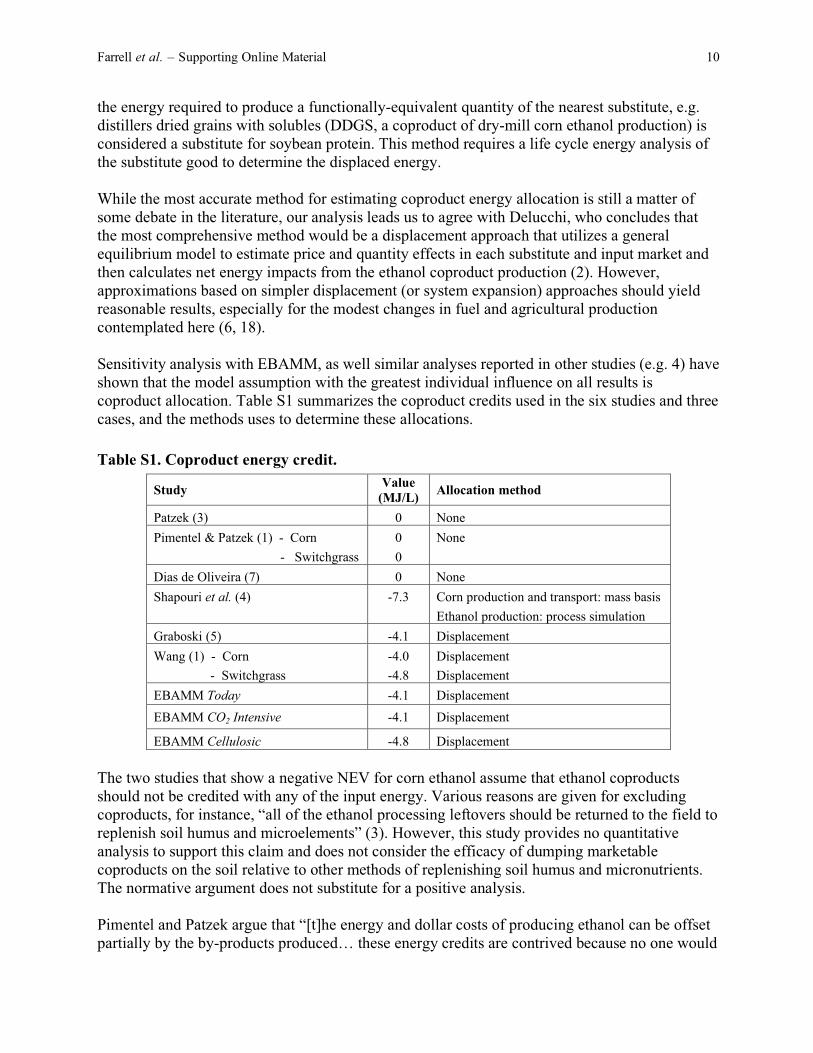
the energy required to produce a functionally-equivalent quantity of the nearest substitute, e.g. distillers dried grains with solubles (DDGS, a coproduct of dry-mill corn ethanol production) is considered a substitute for soybean protein. This method requires a life cycle energy analysis of the substitute good to determine the displaced energy. While the most accurate method for estimating coproduct energy allocation is still a matter of some debate in the literature, our analysis leads us to agree with Delucchi, who concludes that the most comprehensive method would be a displacement approach that utilizes a general equilibrium model to estimate price and quantity effects in each substitute and input market and then calculates net energy impacts from the ethanol coproduct production (2). However, approximations based on simpler displacement (or system expansion) approaches should yield reasonable results, especially for the modest changes in fuel and agricultural production contemplated here (6, 18). Sensitivity analysis with EBAMM, as well similar analyses reported in other studies (e.g. 4) have shown that the model assumption with the greatest individual influence on all results is coproduct allocation. Table S1 summarizes the coproduct credits used in the six studies and three cases, and the methods uses to determine these allocations.

Table S1. Coproduct energy credit.

Study Value

(MJ/L) Allocation method

Patzek (3) 0 None

Pimentel & Patzek (1) - Corn

- Switchgrass

0

0

None

Dias de Oliveira (7) 0 None

Shapouri et al. (4) -7.3 Corn production and transport: mass basis

Ethanol production: process simulation

Graboski (5) -4.1 Displacement

Wang (1) - Corn

- Switchgrass

-4.0

-4.8

Displacement

Displacement

EBAMM Today -4.1 Displacement

EBAMM CO2 Intensive -4.1 Displacement

EBAMM Cellulosic -4.8 Displacement

The two studies that show a negative NEV for corn ethanol assume that ethanol coproducts should not be credited with any of the input energy. Various reasons are given for excluding coproducts, for instance, “all of the ethanol processing leftovers should be returned to the field to replenish soil humus and microelements” (3). However, this study provides no quantitative analysis to support this claim and does not consider the efficacy of dumping marketable coproducts on the soil relative to other methods of replenishing soil humus and micronutrients. The normative argument does not substitute for a positive analysis. Pimentel and Patzek argue that “[t]he energy and dollar costs of producing ethanol can be offset partially by the by-products produced… these energy credits are contrived because no one would


actually produce livestock feed from ethanol at great costs in fossil energy and soil depletion” (1). However, this logic reverses the causal chain. Current ethanol plants sell by-products and current designs for celluslosic biorefineries include the use of the combustible fraction of lignin for electricity generation (including offsite sales) and waste heat recovery, much as the pulp and paper industry does today (19). Dias de Oliveira et al. ignore coproduct energy because no satisfactory estimate was available (20). Shapouri et al. employ a hybrid of process methods to allocate input energy between ethanol and its coproducts (4). Energy inputs for corn production and transportation to the ethanol plant is attributed to ethanol according to the portion of crop weight composed of starch. The energy involved in producing ethanol from corn is allocated to ethanol and its coproducts according to the results of a process simulation conducted using ASPEN Plus software. The last two studies use a displacement method. Graboski uses a displacement method to calculate a coproduct credit for the coproducts of both wet- and dry-mill ethanol production (5). This study goes to some lengths to model the effects of increased coproduct production on several potential feed ingredients, using a linear program to minimize cost according to nutritional constraints. GREET calculates coproduct credits for ethanol using a displacement method. In the case of corn, it assumes the coproduct of dry-milling, DDGS, displaces some whole corn and some soybean meal in animal feed, and that the products of wet-milling, corn gluten meal, corn gluten feed, and corn oil, displace whole corn, nitrogen-in-urea, and soy oil (6). In the case of cellulosic ethanol, the displaced product is the grid-based electricity displaced by the generation and export of electricity through lignin combustion in the ethanol plant. The energy value of the coproduct is thus equal to the primary energy that would have been required to generate this electricity, based on the average fuel mix and efficiency of the United States grid. EBAMM adopts the displacement model of (5) in its calculation of coproduct energy credits for corn ethanol production. This model was chosen because of the extensively documented, multi-product, nutritionally- and economically-balanced displacement analysis presented. EBAMM adopts the displacement model of (6) in its calculation of coproduct energy credits for the production of cellulosic ethanol because of its and simplicity.

Regarding Our Use of a Constant Coproduct Credit

Coproduct yield is a function of biorefinery yield (5, p. 34). The precise relationship isn't obvious, however. It seems reasonable that on a per liter basis, coproduct credit should have an inverse relationship with biorefinery yield: lower yield means more corn is required per liter, and more corn means more protein, oil, etc. (However, it is also possible that a lower EtOH yield is due simply to inefficient processing, which could result in less coproduct and more waste.) In any case, in EBAMM, we apply a constant 4.1 MJ/L credit to each study that reports no coproduct credit. This value was computed by Graboski based on a biorefinery yield of 395 L/Mg, whereas Patzek reports a biorefinery yield of 372 L/Mg, and Dias de Oliveira reports 387 L/Mg.


Given the assumption about lower biorefinery yield implying greater coproduct throughput, the 4.1 MJ/L coproduct energy credit would be a slight underestimate for both Patzek and Dias de Oliveira. However, given the uncertainty about how the different yields (which aren’t significantly different in any case) relate to coproduct yield, it seems reasonable to use the 4.1 MJ/L value in each case. Variance in biorefinery yield probably affects process water and effluent restoration as well, although the direction and magnitude of the impacts are unclear and probably dependent on the particular technologies in use. Again, it seems reasonable to use the same value for each given the minor differences in biorefinery yield.

Fossil Fuel Use

To move beyond the usual focus on net energy, EBAMM also calculates the total primary energy from coal, natural gas, and petroleum used to produce one MJ of ethanol. The quantities of primary and embodied input energy reported by each study are attributed to specific primary fuels according to the assumptions from (6) about the specific primary energy inputs for each process. Where (6) does not calculate the specific primary energy inputs, such as for manufacturing farm equipment, we assume that the distribution of primary energy inputs for the U.S. economy as a whole is applicable (21). In order to compare the fossil fuel consumption implications of competing analyses, a consistent platform is constructed in EBAMM by determining the share of primary energy used in material inputs and processes, and applying these shares to the total energy inputs reported in the surveyed studies to estimate the quantities of individual fossil fuels used in ethanol products. However, because the ethanol production process also results in the production of coproducts that displace substitute products that also require fossil fuels, we also consider coproduct fossil fuel credits. As discussed above, the most accurate method to calculate these fossil fuel coproduct credits would be to use a general equilibrium model to calculate the net change in fossil fuel use within a system that included the substitute product markets. Unfortunately, the data needed for this calculation are not readily available. For simplicity and consistency, we approximate the allocation of fossil fuel consumption by using the fraction of net energy allocated to coproducts with the model of (5), as discussed above. Thus, if 15% of the net energy is allocated to coproducts, then 15% of the input of each fossil fuel type is also allocated to coproducts.

Greenhouse Gas Emissions

Net greenhouse gas (GHG) emissions to the atmosphere are calculated, including the fossil carbon in fuels like gasoline and diesel but excluding photosynthetic carbon in ethanol that comes from feedstock crops. None of the studies examined consider soil carbon sequestration, so we do not consider it in EBAMM. However, depending on agronomic practices, soil C sequestration can significantly affect net GHG emissions (22). Thus, for ethanol, net GHG emissions reflect only the emissions from feedstock and fuel production. Because the majority of GHG emissions from gasoline and ethanol occur in different stages of the fuel cycle (end use and


processing, respectively) both stages must be included to make a meaningful comparison. See the figure in the accompanying paper. The greenhouse gases considered in EBAMM are carbon dioxide (CO2), methane (CH4), and nitrous oxide (N2O). Greenhouse gas emissions are aggregated on a carbon dioxide-equivalent (CO2e) basis, using the 100-year global warming potential (GWP) factors for methane and nitrous oxide emissions recommended by the Intergovernmental Panel on Climate Change (23). These values are 1 for CO2, 23 for CH4, and 296 for N2O. Each study sheets calculates GHG emission values using that paper’s energy and material input assumptions values and a set of GHG emission factors derived from GREET (6). A similar step is taken in the worksheets adjusted for commensurability. The three EBAMM cases use the most appropriate data and assumptions from the six studies. In EBAMM, the GHG calculations follow the format of the net energy calculations. For each of the inputs and steps in agricultural production and conversion to ethanol at the biorefinery, the net CO2e emissions are calculated. For many inputs, these emissions are essentially the sum of emissions of CO2 from primary energy use. However, for some inputs the model accounts for other important sources of GHGs. For instance, the use of nitrogen fertilizer results in GHG emissions in two stages: fertilizer manufacture (primarily CO2 emissions from energy use) and fertilizer application (primarily from N2O emissions from nitrification and denitrification processes in soil). In EBAMM, GHG emissions for nitrogen fertilizer are calculated on a per hectare basis as shown in S-8 through S-10 below.

)/()/(

)/(

22

2

haekgCOemissionsrelatedSoilhaekgCOemissionsoductionprFertilizer

haekgCOemissionsfertilizerNitrogen

+= (S-8)

)/(

)/(

)/(

2

2

hakgNratenapplicatioNitrogen

kgNekgCOfactoremissionsingmanufacturFertilizer

haekgCOemissionsoductionprFertilizer

�

= (S-9)

)/(

)/(/

)/(

2

2

hakgNratenapplicatioNitrogen

kgNekgCOfactoremissionsiationdenitrificionNitrificat

haekgCOemissionsrelatedSoil

�

= (S-10)

Similarly, agricultural lime (CaCO3) application results in GHG emissions from both production energy use and in-soil reactions that release carbon as carbon dioxide. These latter emissions are poorly understood and are a significant source of uncertainty. We use the average of emission factors for limestone and dolomite applications recommended in the Revised 1996 IPCC Guidelines for National Greenhouse Gas Inventories, Worksheet 5-5. For other agricultural inputs, data from (6) are used, including pesticides, transportation, and on-farm energy. The estimate of GHG emissions due to irrigation relies on (24) and (6).


Emissions from energy used in the ethanol facility are based on emissions factors for each energy type and combustion technology as given in (6). Where studies reported only total primary energy, emissions have been calculated based on coal and natural gas emissions factors for wet and dry milling facilities and the percentage of ethanol production using each of these methods as reported in (6). While a few of the papers reviewed here provide estimates of the energy embodied in the on-farm and biorefinery capital, primary energy sources are not reported. We base our estimate on the carbon content of the mix of fuels used in the United States economy in total. We use this same emissions factor for other under-specified reported energy data, including process water and seed production (21). As with net energy, GHG emissions from ethanol are compared in EBAMM to the emissions from the production and use of conventional gasoline. We assume near-term production and combustion technology. The additional use of ethanol due to the Energy Policy Act of 2005 is not expected to bring very much unfarmed land into cultivation, although some shifts in production from one crop to another will occur (18). Significantly greater use of biofuels might shift marginal or unused lands into crop production, however, potentially resulting in significant changes in net GHG emissions due to land use changes alone. The possibility of importing ethanol suggests that land use changes as a result of U.S. ethanol use could occur outside of the country, raising concerns about, for instance, the conversion of rainforest into plantations for fuel production (25). Estimating the magnitude of such effects would be very difficult, requiring analysis of land productivity and availability, commodity markets, and other factors, none of which are considered in the studies evaluated here (2). For these reasons, we ignore GHG emissions due to potential changes in land use. We approximate the allocation of GHG emissions using the fraction of net energy allocated to coproducts with the model of (5), as discussed above. Thus, if 15% of the net energy is allocated to coproducts, then 15% of net GHG emissions are also allocated to coproducts. For most factors, this simplifying assumption will be roughly correct, as GHGs track fairly consistently with energy use. However, there is considerable uncertainty associated with the net GHG effects of some emission sources, including agricultural nitrogen and lime applications, and changes in legume (soybean) cropping. More research is needed to resolve these issues (26).

Regarding Lime Application Rate

The reported rates of lime application in the papers we reviewed covered three orders of magnitude. Shapouri (4) reports the lowest lime application rates. An earlier ethanol study by Shapouri et al. (27) showed corn inputs as per the 1991 and 1996 ARMS (Agricultural Resources Management Survey). Lime rate inexplicably drops from 242 lbs/acre in 1991 to 15 lbs/acre in 1996. We contacted Bill McBride, the USDA Economic Research Service scientist responsible for the corn survey, who looked further into these values and concluded they were incorrect due to a programming error.


The highest value is reported by Graboski (5), who identified significant disparities in lime application rate to corn among different USDA documents. To be conservative, Graboski chose the highest reported value, nearly 3,000 lbs/acre, which is much more lime that is assumed in any of the other studies.

The ARMS of the Economic Research Service of USDA shows a weighted average application on the top 10 corn producing states (over 80% of all U.S. corn) of about 1.3 tons/acre (28). However, an older document on "Agricultural Resources and Environmental Indicators" (29) indicates a much lower percentage of acres receiving lime, with a footnote that in 1996 the nature of the question about lime application changed from "Did you apply lime last year" to "Have you ever applied lime on this field", with corresponding jump in the percentage of acres receiving treatment. The later USDA reports mistakenly disregarded this significant change in survey question and report only "percentage of acres receiving lime" and "amount applied". Tim Payne at USDA confirmed the problem and was kind enough to produce a custom report for us (30). Mr. Payne indicated that USDA will be revising future reports accordingly. This error seems to explain the discrepancy noted by Graboski, and invalidates his choice of the high lime application rate. Our calculations based on the custom report from USDA show a 9-state area-weighted average application rate for lime on corn of 417 lbs/acre for the years 1996-2001. Mr. McBride has confirmed that the custom report represents the USDA’s best estimate of the lime application rate to corn. We have thus adopted this value in EBAMM Release 1.1 for the Ethanol Today and CO2 Intensive cases. Consideration of the corn production system adds further uncertainty. Most corn in the U.S. is grown in annual rotation with legumes (31), and liming is typically required only every few years. Further, while soil acidity is largely due to heavy nitrogen use on corn, legumes are the main beneficiaries of liming, as they are more sensitive to soil pH (32). Proper handling of the energy and GHG impacts of liming requires an expansion of system boundaries to consider the entire cropping system, or an arbitrary allocation scheme. None of the studies we examined addresses this issue.

Other Questions about USDA Data

A more subtle issue relates generally to USDA’s reporting of agricultural inputs. They generally report separate averages for the amount of input applied per acre and the percentage of acres treated. However, the product of these, which is nominally the average amount applied across all acreage, is not the same value (in general) obtained by computing this at the field level and then aggregating the single application rate (area weighted of course) to the state, regional, and national levels. Example: Farmer A spreads 200 lbs/acre of lime on 1% of his acres. Farmer B spreads 100 lbs/acre on 3% of his acres. For simplicity, say the farms are the same size. The USDA method of reporting would show average treatment of 150 lbs/acre on 2% of acres, averaging the two metrics individually. Multiplying these together yields an average application rate of 3 lbs/acre.


However, if you multiply first (maintaining the coherence of each cropping "system") you get farmer A applying 2 lbs/acre on average, and farmer B applying 3 lbs/acre, for an overall average of 2.5 lbs/acre. Now assume A spreads 200 lbs/acre on 3% of his acres and B spreads 100 lbs/acre on 1%. The USDA method produces the same 3 lbs/acre, yet the bottom-up approach now averages 3.5 lbs/acre. Is this a significant problem? It depends on the variance of the product of factors. With lime (post 1996) there are 3 factors that must be treated as a system: percent acres ever treated, application rate, and frequency. We are hoping to gain access to the actual survey data to recompute the average application rate from the bottom up, allowing us to ascertain how much skew is introduced by the independent averaging of these dependent factors.

Supporting Text

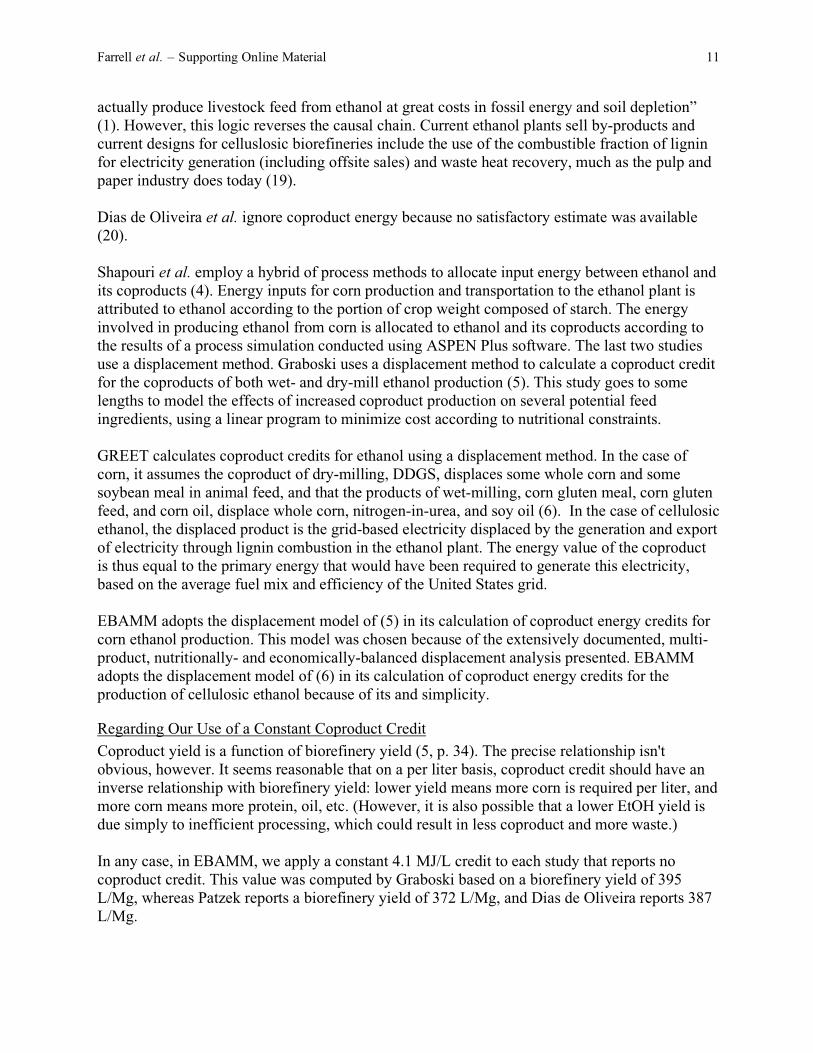
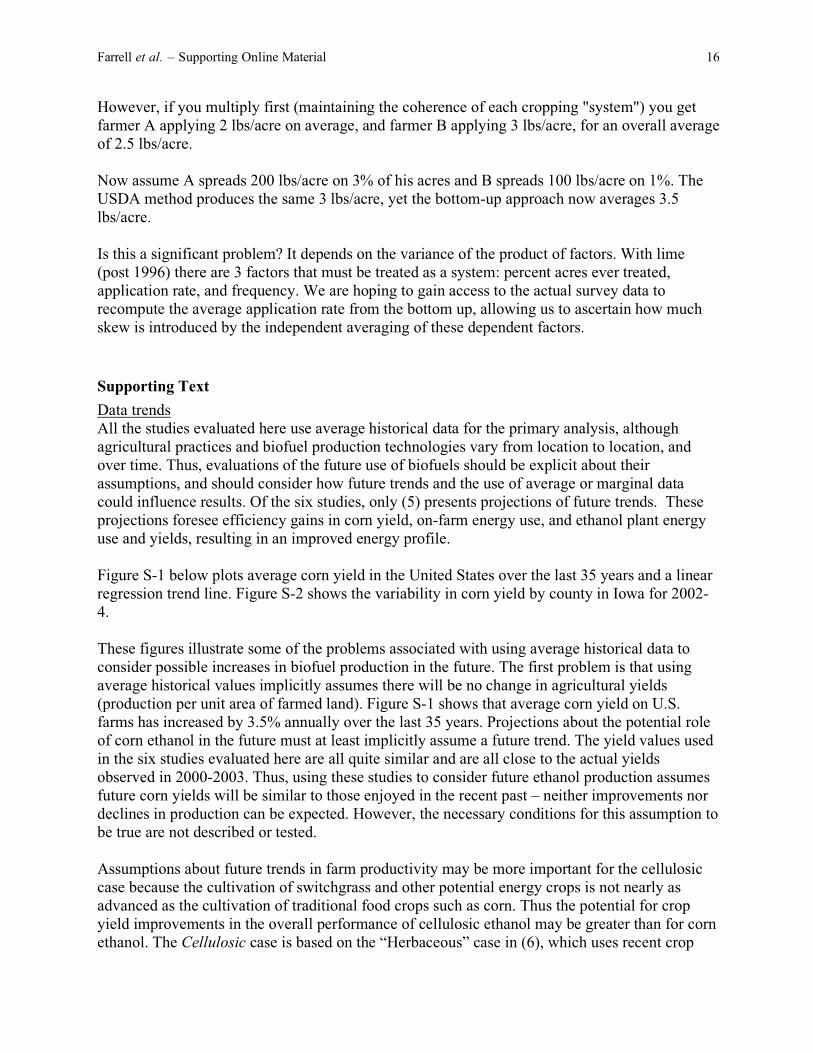
Data trends All the studies evaluated here use average historical data for the primary analysis, although agricultural practices and biofuel production technologies vary from location to location, and over time. Thus, evaluations of the future use of biofuels should be explicit about their assumptions, and should consider how future trends and the use of average or marginal data could influence results. Of the six studies, only (5) presents projections of future trends. These projections foresee efficiency gains in corn yield, on-farm energy use, and ethanol plant energy use and yields, resulting in an improved energy profile. Figure S-1 below plots average corn yield in the United States over the last 35 years and a linear regression trend line. Figure S-2 shows the variability in corn yield by county in Iowa for 2002-4. These figures illustrate some of the problems associated with using average historical data to consider possible increases in biofuel production in the future. The first problem is that using average historical values implicitly assumes there will be no change in agricultural yields (production per unit area of farmed land). Figure S-1 shows that average corn yield on U.S. farms has increased by 3.5% annually over the last 35 years. Projections about the potential role of corn ethanol in the future must at least implicitly assume a future trend. The yield values used in the six studies evaluated here are all quite similar and are all close to the actual yields observed in 2000-2003. Thus, using these studies to consider future ethanol production assumes future corn yields will be similar to those enjoyed in the recent past – neither improvements nor declines in production can be expected. However, the necessary conditions for this assumption to be true are not described or tested. Assumptions about future trends in farm productivity may be more important for the cellulosic case because the cultivation of switchgrass and other potential energy crops is not nearly as advanced as the cultivation of traditional food crops such as corn. Thus the potential for crop yield improvements in the overall performance of cellulosic ethanol may be greater than for corn ethanol. The Cellulosic case is based on the “Herbaceous” case in (6), which uses recent crop


yield data and therefore may underestimate the net energy value of cellulosic ethanol in the future. A second problem is that similar trends exist in conversion yield, which has the added advantage that these improvements are not be subject to environmental constraints (e.g. nutrient loss, soil quality) as agricultural yields are. Scaling up of the ethanol industry will entail additions to ethanol production capacity that will be newer and more advanced than today’s average value, raising average productivity over time. Further, increasing production of ethanol will continue to cause technological innovation and learning-by-doing, as has happened in other industries (33, 34). Because all studies and cases examined here use recent data, they implicitly assume no improvements in biorefinery technologies and thus likely underestimate NEV and petroleum displacement in the future, and overestimate net GHG emissions. Some of the literature on ethanol contains secondary citations which hide the original source and vintage of data that in some cases is obsolete. The importance of trends in agricultural and biorefinery technologies illustrated in Figure S-1 makes this problem especially troubling. (See Table S-4 below.)

Assumed and U.S Average Corn Yield (Mg/ha)

0

2

4

6

8

10

12

1970 1980 1990 2000

Pimentel (2005) Patzek (2004)

Shapouri (2004) de Oliveira (2005)

Graboski (2002) Annual Values

Wang (2001) Linear (Annual Values)

Figure S1: Trend in corn yield and assumed values (35)

A third problem is that the six studies of biofuel production use average national or state estimates for agricultural yield, even though yields vary over a great range for any given crop, as illustrated in Figure S-2. This variability raises several questions: Where will agricultural lands that are shifted into energy production from other uses fall in this distribution? Where in the distribution in yield for current uses does that land currently fall? (That is, What will be the effect of shifting crops from land that is poor for corn but good for switchgrass?) What about idle land that is newly put into production? The ability to analyze these data is limited by the


resolution of available data; further insights from national or even state-level data may be limited and may not be worth pursuing at this time.

Average Corn Yield in Iowa by county, 2002-4

0

5

10

15

20

25

130 135 140 145 150 155 160 165 170 175 180 185 190

Yield (bu/ac)

Nu

mb

er o

f co

un

ties

Figure S2: Variability in corn yield by county in Iowa (35)

Sensitivity Analysis

The relatively simple structure of EBAMM makes uncertainty analysis fairly straightforward. To evaluate the sensitivity of summary values (net energy, net GHG emissions) to the choice of parameter values, we computed the elasticity of the summary value with respect to each input parameter. The elasticity was calculated as the percent change in the summary value given a one percent increase in the input parameter. As elasticities vary with the magnitude of the values considered, there was variance across the studies. However, the analysis yielded a set of parameters that consistently showed the highest elasticities. Although the order sometimes shifted between studies, the top six were consistent across all studies. They are:

• refinery energy (often reported only as an aggregate net energy value) • farm yield • refinery yield • coproduct credit • nitrogen energy • nitrogen application rate

We did not compute elasticities of petroleum consumption with respect to input parameters because there is little petroleum used in ethanol production, and most of it is attributable to the various transportation parameters where liquid fuels are used. In addition, because (2) and (23) suggest that agricultural N2O emissions may be one of the most uncertain parts of this problem, we performed an uncertainty analysis of this factor in our model.


Using the full range of GWP values for N2O reported in (23), net GHG emissions for the Today EBAMM case range from about –10% to +40% relative to the value we report. The upper value includes direct N2O from fertilizer in the soil as well as downstream N2O from applied N that has volatilized and been redeposited elsewhere or leached into water and become N2O later. This sensitivity analysis reflects uncertainties in emissions factors, not uncertainties in N application rates, which do vary by region and county and would have a large impact on total GWP/MJ. However, the uncertainties in the IPCC factors reflect global variation, and the upper end of that range has been critiqued methodologically (26). Moreover, there exist several potential sources of N2O in corn agriculture that are not part of any of the six studies because they focus on energy and not GHGs. For instance, the application of manure, or the incorporation of crop residues (stover) increase N availability, leading to additional N2O emissions. Growing legumes does the same. Because corn is often grown in rotation with soybeans, residual N fixed by soybeans could be partially attributed to corn production because it reduces the need for inorganic sources of N. Finally, the conversion of wetlands to agricultural land is associated with N2O production. Overall, there is deep uncertainty about the net GHG implications of ethanol production (26). The discrepancy in reported lime application rates discussed above under “Regarding Lime Application Rate” as well as the uncertainties in CO2 emissions resulting from lime application prompted us to perform a new uncertainty analysis in EBAMM Release 1.1 with respect to four factors: lime application rate, lime emission factor, nitrogen application rate, and nitrogen emission factor. For lime application rate, we used a lower bound of 18 kg/ha taken from Shapouri et al. (4) and an upper bound of 1121 kg/ha taken from Brees (36), disregarding the Graboski value as reflecting a reporting error at USDA. The emission factor for lime must account for both the energy use in production and delivery, as well as in the relative importance (depending on the soil’s chemical conditions) of reactions of which some release and some absorb carbon dioxide (37). While the chemistry is well understood, the net emissions for any particular field or crop depend on specific soil conditions and agronomic practices, and are therefore highly uncertain overall. For our point estimates, we used the recommended IPCC emissions factors, which assume that 100% of the limestone C is eventually emitted as CO2. However, the fate of limestone carbon is not so certain: CO2 is emitted when limestone is applied to strongly acid soils (pH < 5.0): CaMg(CO3)2 + 4HNO3 � Ca2+ + Mg2+ + 4NO3

- + 2CO2 + 2H2,

but on weakly acid soils (pH 6.5 to 5.0, a range recommended by many agronomists), limestone application results in a net sink of CO2: CaMg(CO3)2 +2H2CO3 � Ca2+ + Mg2+ + 4HCO3

-.


West and McBride recommend that the proper emissions factor is about half of that recommended by the IPCC (37). Initial results from a study of the effect of lime application on GHG emissions in Michigan suggest that in corn agriculture lime may be a net CO2 sink (38). Thus for the uncertainty analysis, we used an upper bound of .44 kg CO2e / kg lime, corresponding to the IPCC factor which assumes that all carbon in lime becomes CO2, and a lower bound of -.22 kgCO2e / kg lime based on Hamilton et al. (38). For nitrogen application rate, we used the full range of values from the studies reviewed, with a lower bound of 146 kg/ha from Dias de Oliveira et al. (7) and an upper bound of 153 kg/ha from Pimentel and Patzek (1). For the nitrogen emission factor, we used the uncertainty range provided by the IPCC discussed above which includes indirect N2O emissions from runoff at the upper end. These values correspond to a lower bound of 1.2 kg CO2e / kg N and an upper bound of 25.4 kg CO2e / kg N. We varied each of these factors in EBAMM Release 1.1 both independently and simultaneously in order to understand their relative contribution to the uncertainty range of greenhouse gas emissions associated with average corn ethanol production. Our Ethanol Today case now yields a point estimate of net greenhouse gases for corn ethanol at 18% below conventional gasoline, but an uncertainty band of –36% to +29%. Note that this band reflects plausible values for average corn production, not merely the range observed across different locations and practices. The largest single uncertainty is in the N2O emission factor, however interactions between nitrogen application and liming are not included in this analysis. These analyses suggest two key implications. First, we can state with reasonable confidence that corn ethanol (or ethanol from other feedstock crops that rely on large amounts of N fertilizer) is unlikely to provide significant reductions in net GHG emissions relative to gasoline, while cellulosic ethanol is likely to provide significant reductions. Second, relatively little petroleum is used to produce ethanol from either corn or cellulosic material, so using ethanol as a transportation fuel reduces petroleum supply requirements.

EBAMM cases

In order to evaluate the importance of assumptions about trends and average values in the analysis of ethanol, three EBAMM cases were created: Ethanol Today, CO2 Intensive, and Cellulosic. System boundaries for these cases were selected to make them commensurate with the adjusted values for the six papers using the best available data. Thus, data from (5) are used for the energy embodied in farm machinery and inputs packaging, and data from (1) are used for the energy embodied in the biorefinery, process water use, and effluent restoration. The Ethanol Today scenario assumes typical current practices for corn ethanol, including the current mix of wet and dry milling, current crop and ethanol yields, and current input (e.g. nitrogen fertilizer) energy intensities. Most of the data are taken from (6). While the Ethanol

Today scenario need not be (and we think is not likely to be) representative of future ethanol


production, it is useful as a benchmark for comparison across studies, because it is uses the most reliable data and requires the fewest additional assumptions. The CO2 Intensive scenario uses the same assumptions as the Ethanol Today case except that the corn production data is for the most energy-intensive major producing state in 2001, Nebraska, and the corn is assumed to be shipped by rail to a lignite-fueled ethanol plant in North Dakota. This scenario is based on a project currently under construction and is meant to illustrate the sensitivity of model results to two significant parameters that could be affected by a major expansion of corn-based ethanol production: the expansion of corn-growing on more marginal lands, and fuel-switching in ethanol production (39). The Cellulosic scenario uses data found in (6) for the production of ethanol from switchgrass, and is adjusted to be consistent with the system boundaries used by EBAMM.

Errors, Omissions, and Inconsistencies

The construction of EBAMM required extensive, detailed examination of the six studies we evaluated, which brought to light some errors, omissions, and inconsistencies in the data. Those that we consider significant are shown in Table S2 below, and described in the associated notes.

Table S2. Errors, Omissions, and Inconsistencies

Source Parameter Problem Note

(3) Ethanol yield Inconsistent data 1

(3) On-farm labor Invalid assumption and double counting 2

(1) Nitrogen fertilizer production energy Misreported data 3

(1) Embodied energy of ethanol plant capital

Obsolete, unverifiable, misreported and inconsistently used data

4

(1) Embodied energy in farm equipment Obsolete, unverifiable data 5

(1) Herbicide application Misreported data 6

(1) On-farm labor Invalid assumption 7

(1) Steam and electricity use in corn ethanol production

Obsolete, inaccurately cited data 8

(1) Steam and electricity use in cellulosic ethanol production

Unsupported assumption

9

(1) Cellulosic ethanol conversion efficiency Obsolete, inaccurately cited data 10

(1) Phosphorus, Potassium, Lime, herbicide, insecticide, farm input transportation

Questionable, unverifiable data 11

(7) Seed energy Incorrect citation 12

(27) All Table 1 N fertilizer values Incorrect unit conversions 13


Explanatory notes for Table S2

1. Pages 523 and 560 report a theoretical maximum ethanol conversion yield from typical,

15%-moisture corn (2.42 gal/kg) that is below the actual average industry yields reported by USDA (based on industry surveys) for both dry and wet milling operations (2.5 and 2.8 gal/bu respectively; weighted average of 2.68 gal/bu) (27). The practical yield of ethanol from moist corn reported in (3) (0.32 L/kg corn) is 20% below the actual recorded average yield of all US ethanol plants in 1998 (0.39 L/kg moist corn).

2. Page 529 presents an estimate of on-farm labor energy input as a fraction of the caloric intake

of workers. Although calculated slightly differently from (1), this approach is also based on the invalid assumption that that a portion of an average corn production worker’s annual caloric intake can be counted as an energy input to corn production. In addition, in (3) this figure is added to a labor energy value from (27). Because both of these figures are derived from USDA NASS labor data, (3) is in effect counting labor energy twice.

3. Table 1 reports N fertilizer energy as 2,448,000 kcal for 153 kg N, which converts to 66.9

MJ/kg and refers to (3) as the source. However (3) reports only 54.4 MJ/kg. This higher value is 23% greater than the cited source, and 13% greater than next highest reported value among studies reviewed here.

4. Table 2 presents data from (1) for the energy embodied in stainless steel, structural steel, and

cement. These data are cited as taken from (40). No calculations or references are given for these values in (40), and these values cannot be checked or verified. Further, in (1) these data are either incorrectly reported or adjusted in an unreported and inconsistent way. Of the 15 instances these values are used in (1), ten data are significantly different than those used in (40). These problems are illustrated below. Values reported in (40):

Stainless steel (pipe) 68 MJ/kg Structural steel 50 MJ/kg Cement 8 MJ/kg

Values reported in (1) said to be based on (40):

Corn ethanol plant: Stainless Steel 17 MJ/kg Steel 17 MJ/kg Cement 4 MJ/kg Cellulosic ethanol plant: Stainless Steel 63 MJ/kg Steel 64 MJ/kg Cement 8 MJ/kg Biodiesel plant: Stainless Steel 60 MJ/kg Steel 49 MJ/kg Cement 8 MJ/kg


5. See discussion of Farm Machinery on page 7. 6. Table 2 reports an herbicide application rate of 6.2 kg/ha, citing a website entitled "History of

U.S. Corn Production." This website contains two sentences relating to pesticide use, citing data from ten and twenty years previous, “Total and per acre use of pesticides for all crops

reached their peak in the early 1980's and has since declined (ERS, 1994). Corn accounted

for 55% of the 410 millions pounds of herbicides used in 1986.” (41) These data do not support the value given in (3). The USDA's "historical track records" indicate that in 1986, 30.5 million acres of corn were harvested (35). Dividing this area into the herbicide application reported above yields an average application of 3.4 kg/ha. The value reported in (3) is 82% larger than this, and more than double the next highest value reported in any of the other studies reviewed here, and no explanation is given for the difference.

7. Table 1 reports energy input of on-farm labor, assuming that a portion of an average corn

production worker’s annual caloric intake can be counted as an energy input to corn production. However, the majority of this food energy would have been consumed by the worker anyway no matter what their employment. Therefore, this assumption is invalid. Furthermore, if the assumption were valid, counting the non-renewable energy input into labor as caloric intake is incorrect. To quantify the energy input into labor, it would be more appropriate to consider the life cycle non-renewable inputs to food production rather than the caloric energy of the food itself. But we believe this to be moot.

8. The citation used in the notes to Tables 2 and 5 for energy for ethanol production is a website listed as "Illinois Corn Growers Association 2004," whereas the actual source is over a decade older (42) and which is available in an updated version at www.ilsr.org.

9. On page 68, (1) argues that although “[t]he energy and dollar costs of producing ethanol can

be offset partially by the by-products produced… these energy credits are contrived because no one would actually produce livestock feed from ethanol at great costs in fossil energy and soil depletion.” As noted earlier, current ethanol plants do, if fact, sell by-products and current designs for celluslosic biorefineries include the use of the combustible fraction of lignin for electricity generation (including offsite sales) and waste heat recovery.

10. In the notes for Table 5, recent claims by an ethanol technology vendor (Arkenol) that 2 kg

of wood cellulose are needed to produce one liter of ethanol is rejected in part because “Others are reporting 13.2 kg of wood per liter of ethanol (DOE, 2004).” This citation is a website (www.eere.energy.gov/biomass/dilute_acid.html) that includes in its first paragraph the following text:

“…As indicated earlier, the first attempt at commercializing a process for ethanol from wood was done in Germany in 1898. It involved the use of dilute acid to hydrolyze the cellulose to glucose, and was able to produce 7.6 liters of ethanol per 100 kg of wood waste (18 gal per ton). The Germans soon developed an industrial process optimized for yields of around 50 gallons per ton of biomass…”

The value of 13.2 kg/L reported by (1) is based on this 107-year old data; 100 divided by 7.6 yields the 13.2. While this value is not used in subsequent calculations, it is used as the sole justification for an otherwise arbitrary choice of an important parameter (see the section on


sensitivity analyses above) without being clear about how it was calculated or noting that it is based on obsolete data.

11. In Table 1, numerous reported values lack any citation or explanation, including embodied

energy in: phosphorus, potassium, lime, herbicide and insecticide. Several of these values are 20-50% higher than values reported by other sources.

12. In Table 1, (4) is cited, but the values are from (43) (See note 20). 13. In Table 1, the entire column of Nitrogen Fertilizer Production values is incorrectly

converted from the English-unit version of the paper to SI, using (x BTU/lb) / (948.45 BTU/MJ) / (2.205 lb/kg) to compute MJ/kg. The correct conversion multiplies, rather than divides, the last term, i.e. (x BTU/lb) / (948.45 BTU/MJ) * (2.205 lb/ kg). So, for example, the N energy value reported by the 2002 version of the paper, 18392 BTU/lb is converted to 8.80 MJ/kg when the correct value is 45.75 MJ/kg. However, it appears that totals were converted directly to SI as totals, rather than by adding up the incorrectly converted values. Thus, the reported final results are correct despite the intermediate error.

Figure S3. Energy Inputs and GHG Emissions for Gasoline and Ethanol

Alternative metrics for evaluating ethanol based on the intensity of promary energy inputs (MJ) per MJ of fuel and of net greenhouse gas emissions (kg CO2-equivalent) per MJ of fuel. For gasoline, both petroleum feedstock and petroleum energy inputs are included. “Other” includes nuclear and hydrological electricity generation. Relative to gasoline, ethanol produced today is much less petroleum-intensive but much more natural gas- and coal-intensive. Production of ethanol from lignite-fired biorefineries located farm from where the corn is grown resultls in ethanol with a high coal intensity and a moderate petroleum intensity. Cellulosic ethanol is expected to have an extremely low intensity for all fosisl fuels and a very slightly negative coal intensity due to electricity sales that would displace coal.


Table S3. EBAMM Results

Data for six studies of corn ethanol and three cases using the EBAMM model and published data. Values for gasoline account for coproducts.

Reference EBAMM results for selected studies EBAMM cases

Gasoline Patzek

2004

Pimentel

et al. 2005

de Oliveira

et al. 2005

Shapouri

et al. 2004

Graboski

2002

Wang

2001

Ethanol

Today

CO2

Intensive

Cellulosic

Petroleum inputs (MJ/MJ)

Original values

Commensurate values

1.1

0.26

0.18

0.25

0.24

0.14

0.07

0.04

0.05

0.05

0.06

0.09

0.10 0.04 0.18 0.08

Net GHG emissions (gC/MJ)

Original values

Commensurate values

94

122

99

117

114

99

77

61

64

99

107

71

74

77

91

11

Net energy (MJ/L)

Original values

Commensurate values

-0.24

-5.0

-1.6

-6.1

-3.1

1.6

4.8

8.9

7.9

3.9

3.1

6.9

5.9

4.6

1.3

23

Percent of published net energy

Original values

-

99.5%

99.9%

100.0%

100.0%

100.5%

100.2%

-

-

-

Coproduct credit (MJ/L)

Original values

Commensurate values

-

0

4.1

0

1.9

0

4.1

7.3

7.3

4.1

4.1

4.0

4.0

4.1

4.1

4.8


References

1. D. Pimentel, T. Patzek, Natural Resources Research 14, 65 (March, 2005).

2. M. A. Delucchi, in Institute of Transportation Studies. (University of California, Davis, 2004) pp. 25.

3. T. Patzek, Critical Reviews in Plant Sciences 23, 519 (2004, 2004).

4. H. Shapouri, J. A. Duffield, A. Mcaloon, paper presented at the Corn Utilization and Technology Conference, Indianapolis, June 7-9 2004.

5. M. Graboski, “Fossil Energy Use in the Manufacture of Corn Ethanol” (National Corn Growers Association, 2002).

6. M. Wang, “Development and Use of GREET 1.6 Fuel-Cycle Model for Transportation Fuels and Vehicle Technologies” Tech. Report No. ANL/ESD/TM-163 (Argonne National Laboratory, Center for Transportation Research, 2001).

7. M. E. Dias De Oliveira, B. E. Vaughan, E. J. J. Rykiel, BioScience 55, 593 (July, 2005).

8. The term "Cellulosic" is used because it is the most intuitive even though this case is based on the use of switchgrass (Panicum virgatum), also called "Herbaceous" in (6). Using other crops (e.g. poplar trees) to produce cellulosic ethanol would likely produce different results.

9. NEV is presented only graphically in (2).

10. Conversion from HHV to LHV was performed based on the International Energy Agency convention of multiplying coal and petroleum energy content by 0.95, and natural gas energy content by 0.9.

11. C. J. Cleveland, Energy 30, 769 (2005/4, 2005).

12. D. V. Spitzley, G. A. Keoleian, “Life Cycle Environmental and Economic Assessment of Willow Biomass Electricity: A Comparison with Other Renewable and Non-Renewable Sources” (University of Michigan, 2005).

13. A. E. Boardman, Cost-benefit analysis : concepts and practice (Prentice Hall, Upper Saddle River, NJ, ed. 2nd, 2001), pp. xvi, 526 p.

14. C. Hendrickson, A. Horvath, S. Joshi, L. Lave, Environmental Science & Technology 32, 184A (Apr 1, 1998).

15. According to the USDA, capital recover for machinery and equipment for corn production in 1997 was $64.50/acre. See http://www.ers.usda.gov/data/costsandreturns/testpick.htm.

16. In the EBAMM study sheets, this occurs in rows 46-49, below the Biorefinery Phase data.

17. S. Kim, B. Dale, International Journal of Life Cycle Assessment 7, 237 (2002).

18. Food and Agricultural Policy Research Institute, “Implications of Increased Ethanol Production for U.S. Agriculture” (University of Missouri, 2005).


19. C. E. Wyman, Biotechnology Progress 19, 254 (Mar-Apr, 2003).

20. M. E. Dias De Oliveira, pers. comm. with R. J. Plevin, August 31, 2005.

21. Energy Information Administration, “Annual Energy Review 2004” Tech. Report No. DOE/EIA-0384(2004) (DC, 2005).

22. R. Lal, Science 304, 1623 (June 11, 2004, 2004).

23. Intergovernmental Panel on Climate Change, Third Assessment Report: The Scientific Basis (Cambridge University Press, New York, 2001), pp.

24. National Agricultural Statistics Service, “Farm and Ranch Irrigation Survey (2003)” Tech. Report No. AC-02-SS-1 (U.S. Department of Agriculture, 2004).

25. G. Monbiot, “The most destructive crop on earth is no solution to the energy crisis,” The Guardian, December 6 2005.

26. A. E. Farrell, A. R. Brandt, A. C. Kerr, M. S. Torn, “Research Roadmap for Greenhouse Gas Inventory Methods” Tech. Report No. CEC-500-2005-097 (California Energy Commission - PIER Program, 2005).

27. H. Shapouri, J. A. Duffield, M. Wang, “The Energy Balance of Corn Ethanol: An Update” Tech. Report No. AER-814 (US Department of Agriculture, 2002).

28. See the "Fertilizer Use and Practices" data for 1998, 1999, and 2000 that are available on http://www.ers.usda.gov/briefing/agchemicals/questions/nmqa3.htm, which indicate a weighted average application rate for lime on corn of over 1 ton per acre.

29. See http://www.ers.usda.gov/publications/arei/ah722/arei4_4/AREI4_4nutrientmgt.pdf

30. The custom report and our lime rate spreadsheet are available at http://rael.berkeley.edu/EBAMM

31. S. Deberkow, H. Taylor, W. Huang, “Agricultural Resources and Environmental Indicators: Nutrient Use and Management” Tech. Report No. AH722 (2000).

32. P. Kassel, J. E. Sawyer, D. Haden, D. Barker, "Soil pH and Corn-Soybean Rotation Yield Responses to Limestone Application and Tillage", http://extension.agron.iastate.edu/soilfertility/info/kasselnwlime00ncextconf.pdf, (accessed 18 Feb 2006).

33. D. Epple, L. Argote, K. Murphy, Operations Research 44, 77 (Jan-Feb, 1996).

34. M. R. Taylor, E. S. Rubin, D. A. Hounshell, Technological Forecasting and Social Change 72, 697 (2005).

35. National Agricultural Statistics Service, “Historical Track Records” (U.S. Department of Agriculture, 2005).

36. M. Brees, "Corn and Irrigated Corn Budgets for Northern, Central and Southwest Missouri", http://www.agebb.missouri.edu/mgt/budget/fbm-0101.pdf, (University of Missouri Dept. of Agricultural Economics, accessed 5/9/2006).


37. T. O. West, A. C. McBride, Agriculture, Ecosystems & Environment 108, 145 (2005).

38. S. K. Hamilton, A. L. Kurzman, C. Arango, L. Jin, G. P. Robertson. (Michigan State University, 2005).

39. Red Trail Energy LLC broke ground in July 2005 on a 50-miilion-gallon/year-capacity plant to be powered by lignite coal. See www.redtrailenergy.com.

40. M. Slesser, C. Lewis, Biological Energy Resources (Halstead., New York, 1979), pp.

41. The cited webpage is defunct, but appears here, courtesy of the Internet Archive: http://web.archive.org/web/20040218051920/http://citv.unl.edu/cornpro/html/history/history.html.

42. D. Morris, I. Ahmed, “How Much Energy Does it Take to Make a Gallon of Ethanol?” (Institute for Local Self-Reliance, 1992).

43. D. Pimentel, Natural Resources Research 12 (June, 2003).

Ethanol Can Contribute to Energyand Environmental GoalsAlexander E. Farrell,1* Richard J. Plevin,1 Brian T. Turner,1,2 Andrew D. Jones,1 Michael O’Hare,2

Daniel M. Kammen1,2,3

To study the potential effects of increased biofuel use, we evaluated six representative analysesof fuel ethanol. Studies that reported negative net energy incorrectly ignored coproducts and usedsome obsolete data. All studies indicated that current corn ethanol technologies are much lesspetroleum-intensive than gasoline but have greenhouse gas emissions similar to those of gasoline.However, many important environmental effects of biofuel production are poorly understood.New metrics that measure specific resource inputs are developed, but further research intoenvironmental metrics is needed. Nonetheless, it is already clear that large-scale use of ethanolfor fuel will almost certainly require cellulosic technology.

Energy security and climate change im-

peratives require large-scale substitu-

tion of petroleum-based fuels as well as

improved vehicle efficiency (1, 2). Although

biofuels offer a diverse range of promising

alternatives, ethanol constitutes 99% of all

biofuels in the United States. The 3.4 billion

gallons of ethanol blended into gasoline in

2004 amounted to about 2% of all gasoline

sold by volume and 1.3% (2.5 � 1017 J) of its

energy content (3). Greater quantities of eth-

anol are expected to be used as a motor fuel in

the future because of two federal policies: a

/0.51 tax credit per gallon of ethanol used as

motor fuel and a new mandate for up to 7.5

billion gallons of Brenewable fuel[ to be used

in gasoline by 2012, which was included in the

recently passed Energy Policy Act (EPACT

2005) (4, 5).

Thus, the energy and environmental impli-

cations of ethanol production are more impor-

tant than ever. Much of the analysis and public

debate about ethanol has focused on the sign

of the net energy of ethanol: whether manu-

facturing ethanol takes more nonrenewable

energy than the resulting fuel provides (6, 7).

It has long been recognized that calculations

of net energy are highly sensitive to assump-

tions about both system boundaries and key

parameter values (8). In addition, net energy

calculations ignore vast differences between

different types of fossil energy (9). Moreover,

net energy ratios are extremely sensitive to

specification and assumptions and can produce

uninterpretable values in some important cases

(10). However, comparing across published

studies to evaluate how these assumptions af-

fect outcomes is difficult owing to the use of

different units and system boundaries across

studies. Finding intuitive and meaningful re-

placements for net energy as a performance

metric would be an advance in our ability to

evaluate and set energy policy in this impor-

tant arena.

To better understand the energy and environ-

mental implications of ethanol, we surveyed the

published and gray literature and present a

comparison of six studies illustrating the range

of assumptions and data found for the case

of corn-based (Zea mays, or maize) ethanol

(11–16). To permit a direct and meaningful

comparison of the data and assumptions across

the studies, we developed the Energy and

Resources Group (ERG) Biofuel Analysis Meta-

Model (EBAMM) (10). For each study, we

compared data sources and methods and param-

eterized EBAMM to replicate the published

net energy results to within half a percent. In

addition to net energy, we also calculated

metrics for greenhouse gas (GHG) emissions

and primary energy inputs (table S1 and Fig. 1).

Two of the studies stand out from the others

because they report negative net energy values

and imply relatively high GHG emissions and

petroleum inputs (11, 12). The close evaluation

required to replicate the net energy results showed

that these two studies also stand apart from the

others by incorrectly assuming that ethanol

coproducts (materials inevitably generated when

ethanol is made, such as dried distiller grains with

solubles, corn gluten feed, and corn oil) should

not be credited with any of the input energy and

by including some input data that are old and

unrepresentative of current processes, or so

poorly documented that their quality cannot be

evaluated (tables S2 and S3).

Sensitivity analyses with EBAMM and else-

where show that net energy calculations are

most sensitive to assumptions about coproduct

allocation (17). Coproducts of ethanol have

positive economic value and displace compet-

ing products that require energy to make. There-

fore, increases in corn ethanol production to

meet the requirements of EPACT 2005 will

lead to more coproducts that displace whole

corn and soybean meal in animal feed, and the

energy thereby saved will partly offset the en-

ergy required for ethanol production (5, 18).

The studies that correctly accounted for this

displacement effect reported that ethanol and

coproducts manufactured from corn yielded a

positive net energy of about 4 MJ/l to 9 MJ/l.

The study that ignored coproducts but used

recent data found a slightly positive net energy

for corn ethanol (13). However, comparisons

of the reported data are somewhat misleading

because of many incommensurate assumptions

across the studies.

We used EBAMM to (i) add coproduct

credit where needed, (ii) apply a consistent

system boundary by adding missing param-

eters (e.g., effluent processing energy) and

dropping extraneous ones (e.g., laborer food

energy), (iii) account for different energy types,

and (iv) calculate policy-relevant metrics (19).

Figure 1 shows both published and commensu-

rate values as well as equivalent values for the

reference, conventional gasoline.

The published results, adjusted for commen-

surate system boundaries, indicate that with

current production methods corn ethanol dis-

places petroleum use substantially; only 5 to

26% of the energy content is renewable. The

rest is primarily natural gas and coal (Fig. 2).

The impact of a switch from gasoline to

ethanol has an ambiguous effect on GHG

emissions, with the reported values ranging

from a 20% increase to a decrease of 32%.

These values have their bases in the same

system boundaries, but some of them rely on

data of dubious quality. Our best point

estimate for average performance today is that

corn ethanol reduces petroleum use by about

95% on an energetic basis and reduces GHG

emissions only moderately, by about 13%.

Uncertainty analysis suggests these results are

robust (10). It is important to realize that actual

performance will vary from place to place and

that these values reflect an absence of incen-

tives for GHG emission control. Given ade-

quate policy incentives, the performance of

corn ethanol in terms of GHG emissions can

likely be improved (20). However, current data

suggest that only cellulosic ethanol offers large

reductions in GHG emissions.

The remaining differences among the six

studies are due to different input parameters,

which are relatively easy to evaluate within the

simple, transparent EBAMM framework. For

instance, most of the difference between the

highest and lowest values for GHG emissions

in our data are due to differences in limestone

(CaCO3) application rate and energy embodied

in farmmachinery (table S1). The former is truly

uncertain; data for lime application and for the

resulting GHG emissions are poor (15). In

contrast, the higher farmmachinery energy values

are unverifiable and more than an order of

magnitude greater than values reported elsewhere

and calculated here, suggesting that the lower

values are more representative (10) (table S3).

This analysis illustrates the major con-

tribution of agricultural practices to life-cycle

GHG emissions (34% to 44%) and petroleum

inputs (45% to 80%) to corn ethanol, suggest-

1Energy and Resources Group, 2Goldman School of PublicPolicy, 3Renewable and Appropriate Energy Laboratory,University of California, Berkeley, CA 94720–3050, USA.

*To whom correspondence should be addressed. E-mail:[email protected]

REPORTS

27 JANUARY 2006 VOL 311 SCIENCE www.sciencemag.org506

ing that policies aimed at reducing environ-

mental externalities in the agricultural sector

may result in significantly improved environ-

mental performance of this fuel. For example,

conservation tillage reduces petroleum con-

sumption and GHG emissions as well as soil

erosion and agrichemical runoff (20, 21).

We use the best data from the six studies to

create three cases in EBAMM: Ethanol Today,

which includes typical values for the current

U.S. corn ethanol industry and requires the

fewest assumptions; CO2Intensive, which has

its basis in current plans to ship Nebraska corn

to a lignite-powered ethanol plant in North

Dakota (22); and Cellulosic, which assumes that

production of cellulosic ethanol from switch-

grass becomes economic as represented in one

of the studies (16).

The Cellulosic case presented here is a pre-

liminary estimate of a rapidly evolving technol-

ogy and is designed to highlight the dramatic

reductions in GHG emissions that could be

achieved. In addition, other biofuel technologies

and production processes are in active develop-

ment and, as the data become available, should

be the subject of similar energy and environ-

mental impact assessments.

For all three cases, producing one MJ of

ethanol requires far less petroleum than is re-

quired to produce one MJ of gasoline (Fig. 2).

However, the GHG metric illustrates that the

environmental performance of ethanol varies

greatly depending on production processes. On

the other hand, single-factor metrics may be

poor guides for policy. With the use of the

petroleum intensity metric, the Ethanol Today

case would be slightly preferred over the Cel-

lulosic case (a petroleum input ratio of 0.06

compared with 0.08); however, on the GHG

metric, the Ethanol Today case is far worse

than Cellulosic (83 compared to 11). Additional

environmental metrics are now being devel-

oped for biofuels, and a few have been applied

to ethanol production, but several key issues

remain unquantified, such as soil erosion and

the conversion of forest to agriculture (18, 20).

Looking to the future, the environmental

implications of ethanol production are likely to

grow more important, and there is a need for a

more complete set of policy-relevant metrics.

In addition, future analysis of fuel ethanol

should more carefully evaluate ethanol pro-

duction from cellulosic feedstocks, not least

because cellulosic ethanol production is un-

dergoing major technological development and

because the cultivation of cellulosic feedstocks

is not as far advanced as corn agriculture,

suggesting more potential for improvement.

Such advances may enable biomass energy to

contribute a sizeable fraction of the nation_stransportation energy, as some studies have

suggested (23, 24).

Our study yields both research and policy

recommendations. Evaluations of biofuel policy

should use realistic assumptions (e.g., the

inclusion of coproduct credits calculated by a

Fig. 1. (A) Net energy and net greenhouse gases for gasoline, six studies, andthree cases. (B) Net energy and petroleum inputs for the same. In these figures,small light blue circles are reported data that include incommensurateassumptions, whereas the large dark blue circles are adjusted values that useidentical system boundaries. Conventional gasoline is shown with red stars, andEBAMM scenarios are shown with green squares. Adjusting system boundaries

reduces the scatter in the reported results. Moreover, despite large differences innet energy, all studies show similar results in terms of more policy-relevantmetrics: GHG emissions from ethanol made from conventionally grown corn canbe slightly more or slightly less than from gasoline per unit of energy, butethanol requires much less petroleum inputs. Ethanol produced from cellulosicmaterial (switchgrass) reduces both GHGs and petroleum inputs substantially.

Fig. 2. Alternative metrics forevaluating ethanol based onthe intensity of primary en-ergy inputs (MJ) per MJ of fueland of net greenhouse gasemissions (kg CO2-equivalent)per MJ of fuel. For gasoline,both petroleum feedstock andpetroleum energy inputs areincluded. ‘‘Other’’ includes nu-clear and hydrological elec-tricity generation. Relative togasoline, ethanol produced to-day is much less petroleum-intensive but much more naturalgas– and coal-intensive. Pro-duction of ethanol from lignite-fired biorefineries located farfrom where the corn is grownresults in ethanol with a high coal intensity and a moderate petroleum intensity. Cellulosic ethanol is expected to have an extremely low intensity forall fossil fuels and a very slightly negative coal intensity due to electricity sales that would displace coal.

REPORTS

www.sciencemag.org SCIENCE VOL 311 27 JANUARY 2006 507

displacement method), accurate data, clearly de-

fined future scenarios, and performance metrics

relevant to policy goals like reducing greenhouse

gas emissions, petroleum inputs, and soil ero-

sion. Progress toward attaining these goals will

require new technologies and practices, such as

sustainable agriculture and cellulosic ethanol

production. Such an approach could lead to a

biofuels industry much larger than today_s that,in conjunction with greater vehicle efficiency,

could play a key role in meeting the nation_senergy and environmental goals.

References and Notes1. T. E. Wirth, C. B. Gray, J. D. Podesta, Foreign Aff. 82, 132

(2003).2. R. A. Kerr, R. F. Service, Science 309, 101 (2005).3. S. C. Davis, S. W. Diegel, Transportation Energy Data

Book (Technical Report No. ORNL-6973, Oak RidgeNational Laboratory, Oak Ridge, TN, 2004).

4. If only cellulosic ethanol production capacity is added,only 4.8 billion gallons will be required because ofpreferential credit provisions.

5. ‘‘Implications of Increased Ethanol Production for U.S.Agriculture’’ (Report No. 10-05, Food and AgriculturalPolicy Research Institute, Univ. of Missouri, Columbia, MO,2005). Also available at www.fapri.missouri.edu/outreach/publications/2005/FAPRI_UMC_Report_10_05.pdf.

6. By convention, photosynthetic energy is ignored in thiscalculation.

7. H. Shapouri, J. A. Duffield, M. Wang, Trans. ASAE 46, 959(2003).

8. R. S. Chambers, R. A. Herendeen, J. J. Joyce, P. S. Penner,Science 206, 789 (1979).

9. C. J. Cleveland, Energy 30, 769 (2005).10. Materials and methods are available as supporting

material on Science Online. Additional information isavailable, including the working EBAMM model, at http://socrates.berkeley.edu/Èrael/EBAMM.

11. T. Patzek, Crit. Rev. Plant Sci. 23, 519 (2004).12. D. Pimentel, T. Patzek, Nat. Resour. Res. 14, 65 (2005).13. M. E. D. De Oliveira, B. E. Vaughan, E. J. Rykiel,

Bioscience 55, 593 (2005).14. H. Shapouri, A. McAloon, ‘‘The 2001 net energy balance

of corn ethanol’’ (U.S. Department of Agriculture,Washington, DC, 2004). Also available at www.usda.gov/oce/oepnu.

15. M. Graboski, ‘‘Fossil energy use in the manufacture ofcorn ethanol’’ (National Corn Growers Association,Washington, DC, 2002). Also available at www.ncga.com/ethanol/main.

16. M. Wang, ‘‘Development and use of GREET 1.6 fuel-cyclemodel for transportation fuels and vehicle technologies’’(Tech. Rep. ANL/ESD/TM-163, Argonne NationalLaboratory, Argonne, IL, 2001). Also available atwww.transportation.anl.gov/pdfs/TA/153.pdf.

17. S. Kim, B. E. Dale, Int. J. Life Cycle Assess. 7, 237 (2002).18. M. A. Delucchi, ‘‘Conceptual and methodological issues in

lifecycle analyses of transportation fuels’’ (Tech. Rep.UCD-ITS-RR-04-45, Univ. of California, Davis, 2004).Also available at www.its.ucdavis.edu/publications/2004/UCD-ITS-RR-04-45.pdf.

19. Factors eliminated were labor transportation, labor foodenergy, and process water energy. The first two weredeemed outside the system boundaries. Process waterenergy was included in one study but was insufficientlydocumented. Factors added were farm machinery energy,

inputs packaging, and effluent processing energy. Themetric for petroleum use included crude oil used as afeedstock for gasoline, and the metric for GHGsincluded end-use (tailpipe) fossil emissions (10).

20. S. Kim, B. E. Dale, Biomass Bioenergy 29, 426 (2005).21. E. Tegtmeier, M. Duffy, Int. J. Agric. Sustainability 2, 1

(2004).22. More information is available at www.redtrailenergyllc.com.23. R. D. Perlack, L. L. Wright, A. Turhollow, R. Graham,

B. Stokes, D. Erbach, ‘‘Biomass as feedstock for abioenergy and bioproducts industry: The technicalfeasibility of a billion-ton annual supply’’ (Tech. Rep.ORNL/TM-2006/66, Oak Ridge National Laboratory,Oak Ridge, TN, 2005). Also available at http://feedstockreview.ornl.gov/pdf/billion_ton_vision.pdf.

24. L. B. Lave, W. Griffin, H. McLean, Issues Sci. Technol. 18,73 (2001).

25. This research was made possible through support fromthe Energy Foundation and the Karsten FamilyFoundation (both to D.M.K.) and NSF’s Climate DecisionMaking Center at Carnegie Mellon University (SES-034578)(to A.E.F.) and Graduate Research Fellowship program(to A.D.J.). The authors thank J. Thompson, D. Greene,M. DeLucchi, M. Wang, and an anonymous reviewer forassistance and valuable comments.

Supporting Online Materialwww.sciencemag.org/cgi/content/full/311/5760/506/DC1Materials and MethodsSOM TextFigs. S1 and S2Tables S1 to S3References

17 October 2005; accepted 9 January 200610.1126/science.1121416

Optical Detection of DNAConformational Polymorphism onSingle-Walled Carbon NanotubesDaniel A. Heller,1 Esther S. Jeng,2 Tsun-Kwan Yeung,2 Brittany M. Martinez,2

Anthonie E. Moll,2 Joseph B. Gastala,2 Michael S. Strano2*

The transition of DNA secondary structure from an analogous B to Z conformation modulates thedielectric environment of the single-walled carbon nanotube (SWNT) around which it is adsorbed.The SWNT band-gap fluorescence undergoes a red shift when an encapsulating 30-nucleotideoligomer is exposed to counter ions that screen the charged backbone. The transition isthermodynamically identical for DNA on and off the nanotube, except that the propagation lengthof the former is shorter by five-sixths. The magnitude of the energy shift is described by using aneffective medium model and the DNA geometry on the nanotube sidewall. We demonstrate thedetection of the B-Z change in whole blood, tissue, and from within living mammalian cells.

Single-walled carbon nanotubes (1) are

rolled sheets of graphene with nanometer-

sized diameters that possess remarkable

photostablity (2). The semiconducting forms of

SWNTs, when dispersed by surfactants in aqueous

solution, can display distinctive near-infrared

(IR) photoluminescence (3) arising from their

electronic band gap. The band-gap energy is

sensitive to the local dielectric environment

around the SWNT, and this property can be ex-

ploited in chemical sensing, which was recently

demonstrated for the detection of b-D-glucose (4).Among the molecules that can bind to the

surface of SWNTs is DNA, which adsorbs as a

double-stranded (ds) complex (5). Certain DNA

oligonucleotides will transition from the native,

right-handed B form to the left-handed Z form

as cations adsorb onto and screen the nega-

tively charged backbone (6–9). We now show

that an analogous B-to-Z transition for a 30-

nucleotide dsDNA modulates the dielectric

environment of SWNTs and decreases their

near-IR emission energy up to 15 meV. We

have used this fluorescence signal to detect

divalent metal cations that bind to DNA and

stabilize the Z form. The thermodynamics of the

conformational change for DNA both on and off

the SWNT are nearly identical. These near-IR

ion sensors can operate in strongly scattering or

absorbing media, which we demonstrate by de-

tecting mercuric ions in whole blood, black ink,

and living mammalian cells and tissues.

Near-IR spectrofluorometry was performed

on colloidally stable complexes of DNA-

encapsulated SWNTs (DNA-SWNTs) buffered

at a pH of 7.4 and synthesized by the non-

covalent binding to the nanotube sidewall (10)

of a 30–base pair single-stranded DNA (ssDNA)

oligonucleotide with a repeating G-T sequence.

This ssDNA can hydrogen bond with itself to

form dsDNA. Several types of semiconducting

SWNTs are present, but as we show below,

they can be identified by their characteristic

band gaps. The shift in band gap is similar for

each type of SWNT, although there is a diam-

eter dependence. After the addition of divalent

cations, we observed an energy shift in the

SWNT emission with a relative ion sensitivity

of Hg2þ 9 Co2þ 9 Ca2þ 9 Mg2þ, which is

identical for free DNA (Fig. 1A) (11). The shift

can also be observed by monitoring SWNT

photoabsorption bands (fig. S1). The fluores-

cence peak energy traces a monotonic, two-

state equilibrium profile with increasing ionic

strength for each case (12).

The removal of ions from the system via

dialysis returns the emission energy to its initial

value, which is indicative of a completely re-

versible thermodynamic transition (Fig. 1B and

1Department of Chemistry, 2Department of Chemical andBiomolecular Engineering, University of Illinois at Urbana-Champaign, Urbana, IL 61801, USA.

*To whom correspondence should be addressed. E-mail:[email protected]

REPORTS

27 JANUARY 2006 VOL 311 SCIENCE www.sciencemag.org508

supporting online material for - alpha.chem.umb.edu

Documents